Advertiser Learning in Direct Advertising Markets

Abstract

Direct buy advertisers procure advertising inventory at fixed rates from publishers and ad networks. Such advertisers face the complex task of choosing ads amongst myriad new publisher sites. We offer evidence that advertisers do not excel at making these choices. Instead, they try many sites before settling on a favored set, consistent with advertiser learning. We subsequently model advertiser demand for publisher inventory wherein advertisers learn about advertising efficacy across publishers’ sites. Results suggest that advertisers spend considerable resources advertising on sites they eventually abandon—in part because their prior beliefs about advertising efficacy on those sites are too optimistic. The median advertiser’s expected CTR at a new site is 0.23%, five times higher than the true median CTR of 0.045%.

We consider how pooling advertiser information remediates this problem. Specifically, we show that ads with similar visual elements garner similar CTRs, enabling advertisers to better predict ad performance at new sites. Counterfactual analyses indicate that gains from pooling advertiser information are substantial: over six months, we estimate a median advertiser welfare gain of $2,756 (a 15.5% increase) and a median publisher revenue gain of $9,618 (a 63.9% increase).

Keywords: Display advertising, Learning models, Bayesian estimation

1 Introduction

Advertisers seek to place ads with publishers whose readers are potential customers of the advertised goods. In the context of direct buy display advertising, wherein impressions are bundled and sold in large quantities across a myriad of sites, the publisher selection problem is daunting. Because sites differ in their readership and the editorial context in which ads are served, advertisers lacking prior experience with a given site are typically uncertain about the value of placing ads there [18, 28]. This uncertainty creates inefficiencies in ad spending that are amplified by the large number of impressions purchased. A key goal of this paper is to explore the welfare implications of advertiser learning in the face of uncertain advertising response in direct buy advertising markets. Though our emphasis is on direct buy display markets, like contexts include video, television, retail media, print, radio, and other channels where impressions are bundled and advertisers face many advertising options. In each of these settings, advertisers often have little information about the efficacy of the channel until after they commit to a large number of impressions and observe the outcome. Consequently, our objective is to measure the degree of advertiser learning and ascertain the attendant welfare implications (for advertisers and publishers) of potentially miscalibrated initial beliefs about the value of advertising across sites.

In this regard, we make several advances. First, much of the canonical economic theory behind advertiser behavior assumes that advertisers know a priori the value of ad exposures [29, 2, 9, 5]. We do not presume valuations are known ex ante to buying ads on a site, but rather that they must be learned. If advertiser prior beliefs are too optimistic (pessimistic), they will spend too much (little) on ads. With experience, however, their media buys should become more efficient. A nascent and growing literature pertaining to automated advertiser learning approaches has recently appeared [8, 10, 19, 22, 21, 28, 31, 4]. While these approaches imply advertisers should try to learn, they do not seek to i) demonstrate whether advertisers do indeed attempt to learn, ii) measure advertisers’ initial beliefs about advertising efficacy, iii) assess the welfare implications of those initial beliefs, nor iv) explore the potential for an intermediary, such as an agency, to pool information across advertisers. Recently, [26] address point i) in the context of an exchange network and find that more experienced advertisers enjoy greater lift from advertising, consistent with learning. In contrast, our research explicitly models the learning process via a structural learning model, explores the welfare implications, and suggests an approach to improve the efficiency of the media buy.

Second, we consider the setting of a direct buy ad network, as opposed to exchanges [1, 6, 32]. According to eMarketer, direct represents 75% of the annual $130B display ad market, with exchanges representing the balance. In spite of this, most prior research in marketing has focused on exchanges [9]. In exchange settings, single impressions are purchased in real time. In direct settings, impressions are bundled and sold in bulk. Often times, direct inventory is listed and sold at a fixed price. In these environments, advertisers face an overwhelming set of sites from which to choose. After selecting some small subset, advertisers then receive feedback on ad response in batches, after large numbers of impressions are served. For example, in our data, a median of 821,000 impressions are bought in a single purchase.

The differences between fixed price contexts and ad exchanges are consequential for how advertiser learning is modeled. In exchange markets, feedback (in the form of KPIs such as clicks) arrives incrementally by impression. In direct markets, a considerable amount of uncertainty can be resolved after a single purchase, because many impressions are bought at once, and the information about ad efficacy obtained from those impressions overwhelms the prior beliefs. Under these circumstances, finding better priors is far more pressing than when testing and learning at the impression level is possible, because there is little opportunity to explore and exploit using exchange algorithms such as those discussed in [28].

Hence, we seek a scalable approach to enhance advertiser priors in order to improve their outcomes in the context of direct ad networks. We propose a procedure whereby advertisers pool information to improve their prior beliefs about their ad efficacy at new sites. This raises the question of what information to share and how. Conceptually, similar advertisers should evidence similar performance at a given site which, in turn, raises the question of how to measure similarity. One approach is to consider advertising copy or design, with the idea that ads that have similar content should also generate similar responses [34]. Because our advertisements are images, we consider the image similarity of the display advertisements. Specifically, we create a set of concept tags for each ad in our data, and then compute a similarity score for each pair of advertisers based on their associated tags. To improve advertisers’ prior beliefs, we predict their click through rates at new sites as a weighted average of other advertisers’ click through rates, where the weights are given by the advertiser similarity scores. Thus, a third contribution is to build on the cold start literature by using machine learning image recognition techniques in the context of an ad exchange [11, 14, 12, 20, 33].

Owing to our approach to sharing information, a fourth contribution pertains to the literature on the role of agencies in advertising. [9] overview recent research on the agencies involved in display advertising, which emphasizes the incentives of agencies bidding on behalf of advertisers to shade bids or collude. We focus instead on the role of agencies as a potential information sharing mechanism. As agencies observe ads and responses at many sites for many advertisers, it becomes possible for advertisers to pool information. We consider how information sharing can improve advertiser priors leading to more efficient matches between advertisers and publishers.

We collect data from a direct sales ad network that consolidates direct sales display ad inventory across multiple publishers (in this case, the sites are blogs). As is common in the direct sales display advertising channel, advertisers procure the publishers’ ad inventory in advance at a fixed rate. The data from this ad aggregator are ideal for our empirical context, because we observe ad sales and ad prices from the network’s inception and over a long duration (3 years). As a result, the behavior of all advertisers is observed from the aggregator’s infancy, providing an ideal context in which to observe advertisers learning. Our empirical strategy relies upon longitudinal changes in the advertisers’ propensity to choose sites, and this variation is common in our data. The structural learning model we develop presumes that advertisers choose the number of ad impressions across sites to maximize their profits, conditioned on their (possibly incorrect) beliefs about the efficacy of advertising on those sites. After placing an ad, advertisers observe the click-through rates (CTR) at each site. These CTRs provide a noisy signal about the site’s match with the advertiser’s ads. Sites with higher (lower) CTR’s are more (less) likely to be indicative of a good match, and therefore sites with high CTRs are more likely to be used again by the advertiser. In other words, when advertisers select a site upon which to advertise, fail to obtain clicks, and then cease to advertise, we reason they were too optimistic in their initial beliefs about the efficacy of advertising on that site. We then use the demand-side model estimates to gain insights about advertiser conduct, and to simulate demand under counterfactual scenarios that manipulate what advertisers know.

The data evidence patterns that are broadly consistent with learning, as advertisers initially try many sites before settling on a smaller number among which ad response tends to be the greatest. Our initial findings suggest advertisers are overly optimistic in their initial beliefs about the efficacy of advertising. The median advertiser’s choices are consistent with an expected click through rate of 0.23% when, in practice, the median CTR is .045%. We infer from this that advertisers tend to choose the wrong publisher sites initially and overspend on them, while also raising the possibility that advertisers are overlooking sites that would have been a better match. By pooling information, the median advertiser in our estimation sample increases expected total spend by about $671 (52.8%) over six months, and generates an expected incremental $2,756 (15.5%) gain in value. This gain largely arises by ensuring advertisers can sort themselves into publisher sites that are a better match. Owing to this better match, the median publisher also obtains an expected $9,618 (63.9%) increase in revenue over six months (across the top 20 publishers in our data). Projecting these median effects across all advertisers and smaller publishers in the considered ad network would imply an overall welfare gain upper bound of around $14,000,000, and presumably similar gains could accrue to other direct ad networks as well in related contexts such as retail media and online video.

In what follows, we first overview the data and provide descriptive evidence of advertiser learning. We then outline an advertiser learning model, report the estimation results, detail the counterfactual analyses related to information sharing, and conclude with a summary of our findings and ideas for further research.

2 Data

2.1 Data Overview

To assess the effect of advertiser learning, it is necessary to observe the advertising decisions of firms over time. To this end, we have collected data provided by a fixed-price direct-sales Internet ad aggregator. The data span 3 years, starting with the aggregator’s inception in late July 2006 and ending in early December 2009 and covers 8,000 advertisers and 3,200 publishers. These data record the transactions between advertisers and publishers. Each transaction corresponds with an individual advertiser’s ad buy (commonly called a subscription), and specifies the number of consecutive days (typically a week) the ad is to be shown to all visitors to the publisher’s web site, and the price paid by the advertiser for that purchase. Further, for each day the ad is active, the data record the total number of impressions—the number of times the ad was served to a site visitor—and the number of clicks—the number of times a site visitor clicked on the ad. Over the duration of the data, we are aware of no algorithmic changes that might influence the nature of advertiser learning.

For estimation, we focus on a subset of these data. Using k-means clustering with a Jaccard similarity metric computed from the overlap of firms advertising on sites, we identify a subset of 165 politically liberal blogs and news sites serving a similar set of advertisers that do not generally advertise on other sites. This subset of publishers comprises 15.6% of subscriptions (ad buys) in the data, with 1801 (22.7%) of the advertisers in the data placing an ad at one or more of these sites. From this coherent grouping of publishers, we select the top 20 in terms of total ad revenue, limiting attention to the most common ad format and transactions conducted in the first half of 2007 (January 1–June 30). We then choose a random subset of 100 advertisers who placed an ad at one or more of the top 20 sites, and aggregate choices to the weekly level to comport with advertisers’ typical purchase frequency (rarely does interpurchase time fall short of a week). The unit of analysis for our empirical model is thus at the advertiser-site-week level. Over the 27 weeks in the first half of 2007, the estimation sample comprises 547 ad subscriptions. We assume that advertisers include the top 20 sites in their choice sets, unless a previously purchased subscription is already running in a given week. Some advertisers joined the ad network during the estimation window; for these we only consider choices starting with the week they first appear in the data. The estimation sample thus comprises 36,911 choices leading to 547 purchases.

We use the daily number of impressions for each ad (in the period prior to July 2007, including the second half of 2006) to impute the daily average number of ad impressions at each site. This serves as an approximation to sites’ expected daily traffic. The site in the estimation sample with the greatest number of daily visitors had a peak audience of 910K daily visits in the first half of 2007, and average daily traffic of 420K; the site with the least traffic peaked at 43K, with average daily traffic of 20K. Prices vary accordingly, with the most expensive placement garnering over $755 per day ($2265 for 3 days) and the least just $5.50 per day ($500 for 3 months). A typical subscription in our estimation sample lasts one week, costs $800, and yields 821K impressions; the median click-through rate among ads in the estimation sample is 0.045%.

2.2 Descriptive Analyses

In this subsection, we first provide preliminary data analyses to reveal patterns that could be construed as consistent with advertiser learning. Such an analysis affords evidence of the types of behaviors we seek to model. In addition, we characterize how advertising outcomes (CTRs) vary across sites and advertisers. To the extent CTR variation across sites is large relative to CTR variation across advertisers (or site-advertisers), there is value in sharing information about CTRs among advertisers.

2.2.1 Evidence of Advertiser Learning

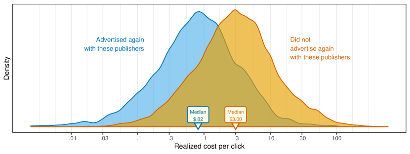
Figure 1: Distribution Of Realized Cost Per Click, Grouped By Action After First Ad Run Is Completed. Based on 1,784 advertisers who ran ads with any publisher in the focal cluster of 165 sites, showing only ads placed by these advertisers at these sites. Cost per click is cumulative through last observed ad placement. Medians are indicated.

Figure 1 shows the distribution of realized cost per click (CPC) for all ads placed at the subset of 165 liberal blogs and news sites by about 1800 advertisers. Because ads are placed on a fixed-price basis, CPC is an outcome that is only observed after the ad has run. Hence, after comparing the number of clicks an ad received with the amount of money spent, the advertiser can calculate the effective CPC for that ad. If the advertiser never used that particular site again, then the realized cost per click is depicted in the distribution on the right of Figure 1 (labeled “Did not advertise again with these publishers”). If the advertiser did place additional ads at that site, then the realized CPC is included in the distribution to the left. The difference between these two distributions is consistent with advertisers abandoning sites where the returns to advertising (as reflected in the ex post number of clicks received) are insufficiently high to justify the cost.

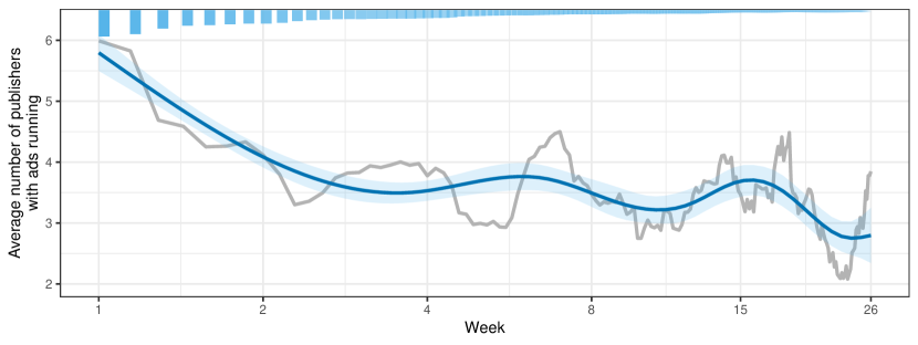
Figure 2: Average Daily Number of Sites Running Ads. The first 26 weeks of ads served by the focal cluster of 165 sites are shown for 939 advertisers who placed ads with two or of these publishers. The line (and smoothed average) depicts the average daily number of publishers serving ads for advertisers actively running ads. The timing of ads is normalized relative to when the advertiser joined the ad network, truncated to show weeks 1–26, and logarithmically scaled to emphasize changes during the initial few weeks of advertising. The number of advertisers with ads running, depicted by the bars at the top of the chart, decreases from 939 in week 1 to 64 in week 26.

Figure 2 provides another view of the data that is consistent with advertiser learning. For each advertiser that placed at least one ad with one of the 165 liberal blogs and news sites, we calculate the number of sites on which the advertiser actively ran ads each day. We then normalize the start dates for these time-series to account for different advertiser cohorts commencing their advertising on different dates (because subscriptions are typically 7 days or more, observations prior to 7 days are truncated). For each day, we calculate the average number of sites actively used by each advertiser, conditional on that advertiser running at least one ad. By the end of the first week after buying their first ad, advertisers have ads running, on average, at about 6 sites. But over the next month, the number of sites used drops by almost half. Moreover, many advertisers cease advertising entirely during this period. By the end of the first week, 939 advertisers are still running ads. By week 26, the number of advertisers still running ads at the subset of 165 sites drops to 64. This pattern is predicted by learning, as advertisers start with a larger set of sites, but eventually stop placing ads at the least effective sites.

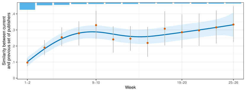
Figure 3: Persistence in Set of Publishers Chosen. The first 26 weeks of ads purchased from the focal cluster of 165 sites are shown for 542 advertisers who placed ads with two or more publishers of these publishers in two or more two-week periods. The timing of ad buys is normalized relative to when the advertiser joined the ad network and truncated to the first 26 weeks. Similarity is calculated as the Jaccard coefficient between i) the set of publishers used in a two-week period, and ii) the set of publishers from the most recent, previous two-week period with an ad buy. Points (vertical lines) indicates the average (bootstrap 95% CI’s) similarity in the set of sites used among advertisers purchasing ads. The number of advertisers purchasing ads, depicted by the bars at the top of the chart, decreases from 407 in weeks 1–2 to 45 in weeks 25–26.

We present a third piece of evidence for advertiser learning in Figure 3, which depicts changes over time in the set of sites at which advertisers place ads. Similarity is calculated as the Jaccard coefficient between i) the set of publishers used in a given two-week period, and ii) the set of publishers used in the most recent prior period where an ad buy took place. This coefficient, defined as the cardinality of the intersection of the two sets divided by the union of the two sets, ranges from 0 to 1, with a higher number meaning that the sets of sites used by the advertiser show greater overlap between the current and preceding buys. Over time, the set of sites an advertiser places ads at is more likely to resemble the previous set of sites where ads were placed as the Jaccard coefficient triples from 0.1 to 0.3.

Thus, not only is the number of sites chosen decreasing, but the decreasing set exhibits greater consistency over time and advertisers tend to advertise more when finding sites that yield better outcomes in terms of click through rates. Collectively, these behaviors would be consistent with finding a set of sites that works well, and sticking with that set.

2.2.2 Evidence of Returns to Learning

Our conjecture is that there exists something for the advertiser to learn. If CTRs are homogenized across sites, then there is little value to learning. Toward this end, we consider a variance decomposition of CTRs across advertisers and sites. Results are shown in Table 1 and suggest that 9% of the variation in CTRs can be apportioned to publishers, 51% to advertisers, and the remainder to advertiser-site match. The 40% of variation apportioned to the advertiser-publisher residual suggests that there is a benefit to advertisers in finding a match with those sites that yield better outcomes.

Term	DF	Sum of Squares	Variation Explained (%)
Advertiser	$1783$	$.0248$	$50.8$
Publisher	$164$	$.0044$	$9.1$
Residuals	$8205$	$.0196$	$40.1$

Table 1: Variance decomposition of advertiser-site long-run click through rates. Based on data from 1784 advertisers who placed one or more ads at the focal set of 165 sites.

3 Model and Estimation

In this section we detail the model of advertisers’ site choice (Section 3.1), and how learning affects these choices (Section 3.2). We conclude by detailing our estimation approach (Section 3.3). We defer our discussion of policy implications, such as the effect of perfect information on advertiser and publisher outcomes to Section 5, where we detail and conduct a number of policy counterfactuals.

3.1 Advertising Payoffs

Each week $w$, advertiser $a$ considers placing an ad at each of the sites, $s$, where an ad is not already running. When choosing to place an ad at site $s$, the advertiser considers a menu of potential run lengths (i.e., how many days the ad is to run), $x$, and prices, $p$, that are charged by sites. For example, the advertiser considering site $s$ might have the following options: $\{$7 days for $100, 14 days for $180, 30 days for $350, not advertising at site $s$$\}$.

The expected payoff generated by the ad running for $x$ days at site $s$ starting at week $w$ depends on the expected number of site visitors who will be exposed to the ad. The average daily number of visitors exposed to ads at site $s$ is denoted $t_{s}$ and is common knowledge to all sites and advertisers. Accordingly, an ad running for $x$ days at site $s$ yields $t_{s}x$ total expected impressions. We specify advertiser $a$’s expected payoff from an ad running for $x$ days at site $s$ as follows:

$$\pi_{asw}\left(x\right)=\delta_{asw}\,\zeta_{a}^{-1}\,\log\left(1+t_{s}x\zeta_{a}\right)-p_{sw}(x)$$ (1)

where the first summand represents the advertiser’s valuation from the expected advertising outcome, and the second ($p_{sw}(x)$) represents the price the publisher charges to the advertiser. This function for advertiser valuation is a special case of the generalized translated constant elasticity of substitution utility function discussed in [7] and [13]. The parameter $\zeta_{a}>0$ determines the rate at which the advertiser satiates on additional impressions. The term $\delta_{asw}>0$ determines the overall scale of payoffs, and in particular the change in marginal payoff at the point of zero impressions.

The term $\delta_{asw}$ is subscripted by both advertiser and site, reflecting the empirical regularity that the same number of impressions served by two similar sites can generate different payoffs for the same advertiser [18]. We refer to this as the match between the advertiser’s ad content and the site’s audience. A high match value leads to higher profits, and thus a higher likelihood of advertising at site $s$. A priori, the value of $\delta_{asw}$ is unknown to the advertiser, but it can be learned over time, as described in Section 3.2. Were the advertiser to be overly optimistic about its match with site $s$, it would initially advertise too much at that site. Were the advertiser to be overly pessimistic, it would advertise too little. Hence, there is value in learning efficiently about match.

As is not uncommon in the context of learning models [17], we assume advertisers are not forward-looking when making choices. Given the difficulty in optimizing learning sequences [21], we doubt whether smaller advertisers could compute and invoke optimal test and learn sequences in this particular setting.

3.2 Advertiser-Site Match and Learning

We next discuss how advertisers learn about their match value with each site. We assume clicks provide an unbiased signal about match under the presumption that more clicks reflect greater interest in the advertised good. Hence, we first link match ($\delta_{asw}$) to clicks ($c_{as}$), and then show how changes in beliefs (i.e., learning) about clicks translate into changes in beliefs about match.

3.2.1 Linking Clicks to Match

We use the proportion of site $s$’s audience who click on advertiser $a$’s ads—that is, the true CTR—as a measure of the general effectiveness of advertiser $a$’s ads when shown to site $s$’s audience. We denote the true CTR $c_{as}$, and note that this rate is unknown to both the advertiser and the site. Conditional on this unknown quantity, the true match between advertiser and site is a function of their true CTR, as given by

$$\delta_{asw}\big{|}c_{as}=\frac{c_{as}}{\gamma_{a}}\exp\left(\xi_{a}+\eta_{s}+\phi_{\tau[a,s,w]}+\psi_{m[w]}+\epsilon_{asw}\right).$$ (2)

As we shall elaborate in the next subsection, the term $c_{as}\big{/}\gamma_{a}$ implies that match values are proportional to the true, but a priori unknown, advertiser-site CTRs.

Although actual CTRs are initially unknown to the advertiser, the component of advertiser match given by $\exp\left(\xi_{a}+\eta_{s}+\phi_{\tau[a,s,w]}+\psi_{m[w]}+\epsilon_{asw}\right)$ is presumed known to the advertiser when choosing where to place ads. This fixed component of advertiser match is decomposed into the following parts. First, the term $\xi_{a}$ reflects the general efficacy of a firm’s advertising across sites and accommodates the possibility that some advertisers purvey goods that are more popular than others, or that the advertiser is endowed with better advertising. Analogously, $\eta_{s}$ reflects differences in sites’ efficacy that are common to all advertisers, perhaps due to the demographics of the site or some aspect of its content or construction. Although, more generally, any ad-site-week observable covariates could be incorporated into the conditional match expression for $\delta_{asw}$, we only observe $\phi_{\tau[a,s,w]}$, a fixed effect that is selected according to how long ago advertiser $a$ first placed an ad at site $s$. Its purpose is to reflect dynamics in the value or efficacy of advertising that are unrelated to learning about match (e.g., wear-in or wear-out; [15]). The term $\psi_{m[w]}$ is a month fixed effect to account for any dynamics affecting the entire ad network. Finally, $\epsilon_{asw}$ is an idiosyncratic demand shifter defined at the advertiser-site-week level that is observed by the advertiser and not the econometrician.

3.2.2 Learning About Clicks

As mentioned, the expression $c_{as}\big{/}\gamma_{a}$ indicates the ratio of advertiser $a$’s true (but a priori unknown) CTR at site $s$ to the parameter $\gamma_{a}$. The parameter $\gamma_{a}$ serves as both i) advertiser $a$’s prior expectation for its unknown CTR at any new site, and ii) the baseline for judging how successful its advertising has been. For example, if the true CTR at site $s$ turns out to be greater than what the advertiser previously expected, then $c_{as}\big{/}\gamma_{a}$ will be greater than $1$, reflecting better returns to advertising at site $s$ than anticipated. To the extent initial beliefs about click through rates are too high (low) at a given site, one would expect advertisers’ initial probabilities of advertising to be higher (lower).

We assume prior beliefs about the true CTR, $c_{as}$, which we denote $\tilde{c}_{as}$, follow a beta distribution, owing to the beta’s flexibility in representing distributions bounded between 0 and 1. Specifically,

$$\tilde{c}_{as}\,\big{|}\,\gamma_{a}\,\sim\mathrm{Beta}\left(1,\left(1-\gamma_{a}\right)\big{/}\gamma_{a}\right),$$ (3)

which implies $\mathbb{E}\left[\tilde{c}_{as}|\gamma_{a}\right]=\gamma_{a}$, and places the bulk of probability density between 0 and about $4\gamma$ (i.e., $\tilde{c}_{as}$, like most CTRs, is a priori skewed towards 0). The parameter $\gamma_{a}$ thus reflects advertiser $a$’s prior belief about its CTR at any previously unused site.

Conditional on the true CTR, $c_{as},$ we assume the likelihood for the cumulative number of clicks as of week $w$, $n_{asw}^{C}$, follows a binomial distribution with likelihood

$$n_{asw}^{C}\,\big{|}\,n_{asw}^{I},c_{as}\,\sim\mathrm{Binomial}\left(n_{asw}^{I},c_{as}\right),$$ (4)

where $n_{asw}^{I}$ is the cumulative number of advertising impressions served. The number of clicks received ($n_{asw}^{C}$) depends on the true CTR at site $s$, $c_{as}$, hence impressions and clicks provide information about the true, but unknown CTR. Accordingly, we specify a Bayesian updating process on advertiser beliefs about the CTR, leading to a beta-binomial posterior CTR belief distribution for the number of clicks. The mean of this updated distribution has an expected value of

$$\mathbb{E}\left[\tilde{c}_{as}\,\big{|}\,n_{asw}^{I},n_{asw}^{C},\gamma_{a}\right]=\gamma_{a}\frac{1+n_{asw}^{C}}{1+\gamma_{a}n_{asw}^{I}}.$$ (5)

Accordingly, the expected ratio of CTR to $\gamma_{a}$ is $\mathbb{E}\left[\tilde{c}_{as}/\gamma_{a}\,\big{|}\,n_{asw}^{I},n_{asw}^{C},\gamma_{a}\right]=(1+n_{asw}^{C})/(1+\gamma_{a}n_{asw}^{I})$.

As previously noted, Equation (5) implies that the advertiser initially expects a CTR of $\mathbb{E}\left[\tilde{c}_{as}\big{|}\gamma_{a}\right]=\gamma_{a}$ before any advertising begins (when $n_{asw}^{C}=0$ and $n_{asw}^{I}=0$). As $n_{asw}^{C}\rightarrow\infty$ and $n_{asw}^{I}\rightarrow\infty$ , the ratio $n_{asw}^{C}/n_{asw}^{I}\rightarrow c_{as}$, and thus $\mathbb{E}\left[\tilde{c}_{as}\big{|}\gamma_{a}\right]\rightarrow c_{as}$. Thus, initial beliefs about the CTR begin as $\gamma_{a}$, but eventually converge to $c_{as}$ with enough advertising. If initial beliefs are correct, this ratio remains at one and never changes (in expectation). If initial beliefs are low (high), this ratio increases (decreases). For example, if the true CTR is less than $\gamma_{a}$, then the number of clicks received, $n_{asw}^{C}$, will grow at a slower rate than the a priori expected number of clicks received, $\gamma_{a}n_{asw}^{I}$, and thus $\gamma_{a}$ in Equation (5) will be multiplied by a ratio that converges to a value between 0 and 1. In the case when initial beliefs are too high, the advertiser spends too much on advertising in early periods and the added expense is not recovered by sales. Conversely, when initial beliefs are too low, advertisers spend too little. Figure 4 illustrates the learning process for click through rates and how these beliefs change over time.

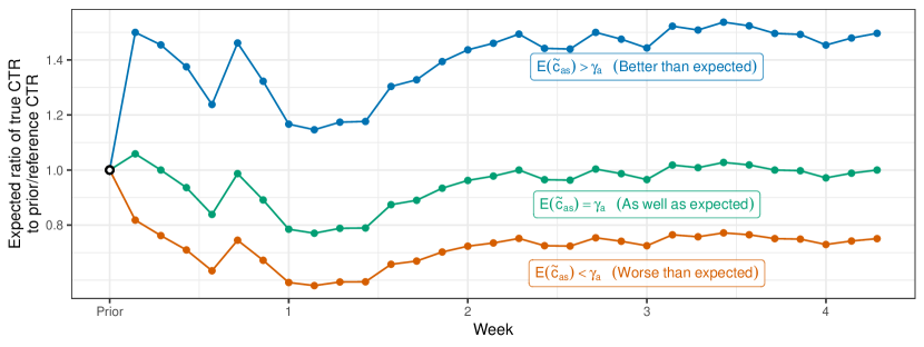
Figure 4: Simulated Posterior CTR Beliefs. The evolution of posterior beliefs for $\mathbb{E}\left[\tilde{c}_{as}/\gamma_{a}\,\big{|}\,n_{asw}^{I},n_{asw}^{C},\gamma_{a}\right]$ is simulated under a true click through rate of $0.0075$. The advertiser prior is either pessimistic (blue plot, $\gamma_{a}=0.005$), accurate (green plot, $\gamma_{a}=0.0075$) or optimistic (red plot, $\gamma_{a}=0.01$).

3.2.3 Learning About Match

The expression for true match values in Equation (2) presumes that the CTR is known. Using the standard beta-binomial distribution as applied to the prior for $\tilde{c}_{as}$ from Equation (3) and the likelihood for $n_{asw}^{I}$ from Equation (4), and taking the expectation of $\delta_{asw}$ with respect to $\tilde{c}_{as}$ in Equation (2), we can express the advertiser’s updated expected match with site $s$, $\tilde{\delta}_{asw}$, as

$$\mathbb{E}\left[\tilde{\delta}_{asw}\,\big{|}\,n_{asw}^{I},n_{asw}^{C},\epsilon_{asw},\theta\right] =\check{\mu}_{asw}\cdot\exp(\epsilon_{asw})$$

$$=\frac{1+n_{asw}^{C}}{1+\gamma_{a}n_{asw}^{I}}\exp\left(\xi_{a}+\eta_{s}+\phi_{\tau[a,s,w]}+\psi_{m[w]}\right)\cdot\exp(\epsilon_{asw}),$$ (6)

where $\theta$ represents the model parameters. Defining $\check{\mu}_{asw}\equiv\mathbb{E}\left[\tilde{\delta}_{asw}\,\big{|}\,n_{asw}^{I},n_{asw}^{C}\right]/\exp(\epsilon_{asw})$ will prove useful when deriving the likelihood function. Combining Equation (6) with Equation (1), where true match is replaced by expected match, yields an expression for expected advertiser payoffs conditional on past impressions ($n_{asw}^{I}$) and clicks ($n_{asw}^{C}$).

3.3 Estimation

We construct the likelihood of the observed data using the method described in [13]. The central idea behind this approach is to derive a set of inequality constraints on $\epsilon$ that rationalize the observed set of choices. For example, if an advertiser buys a 7 day ad run at a given price, the advertiser must have obtained a greater expected payoff than it would have otherwise obtained by buying a different length of ad run at an alternative price. As we observe many advertiser choices over many periods, this yields a large number of inequality constraints from which one can derive a likelihood.

The data (advertiser choices of sites) are observed at the weekly level. Hence, we consider the idiosyncratic demand shifters, $\epsilon_{asw}$, in Equation (6), and their implications for advertiser payoffs given by Equation (1). Replacing the true match with expected match, the expected payoff equation becomes

$$V_{asw}^{\theta}(x,\epsilon_{asw}) \equiv\mathbb{E}\left[\pi_{asw}(x)|\theta,\epsilon_{asw},n_{asw}^{I},n_{asw}^{C}\right]$$

$$=\check{\mu}_{asw}\exp(\epsilon_{asw})\,\zeta_{a}^{-1}\,\log\left(1+t_{s}x\zeta_{a}\right)-p_{sw}(x),$$ (7)

where the set of parameters to estimate is given by $\theta=\{\gamma,\xi,\eta,\phi,\psi,\zeta\}.$ Of special interest in this set is $\gamma$, the vector of advertisers’ prior beliefs about the efficacy of their advertising, which is informative about whether their naivety induces them to advertise too much or too little.

Given a set of parameters $\theta$, the likelihood of $x_{asw}$ is given by the probability density of $\epsilon_{asw}$ integrated over the region of $\epsilon$’s that can rationalize the observed choice of $x_{asw}$. This region is defined by upper and lower bounds, which are themselves determined by a pair of inequality constraints. Let $\shortuparrow\!\!x$ denote an alternative subscription that is longer than the subscription of length $x$ that was purchased, and let $\shortuparrow\!\!p$ denote its (higher) price. Similarly, let $\shortdownarrow\!\!x$ denote an alternative, shorter subscription, and $\shortdownarrow\!\!p$ its (lower) price. Moreover, assume for the moment that both shorter and longer alternatives to $x_{asw}$ were offered by site $s$.

The lower bound for the region of $\epsilon$ that can rationalize $x_{asw}$ is obtained from the observation that the advertiser did not buy the shorter subscription, $\shortdownarrow\!\!x$. Hence, we know $V_{asw}^{\theta}(x,\epsilon_{asw})>V_{asw}^{\theta}(\shortdownarrow\!\!x,\epsilon_{asw})$. Substituting Equation (7) into this inequality and isolating $\epsilon_{asw}$ leads to the following lower bound for $\epsilon_{asw}$ [13]:

$$\epsilon_{asw}>\ell b^{\theta}(x_{asw},p_{sw}),\qquad\ell b^{\theta}(x,p)\equiv\log(p\,-\shortdownarrow\!\!p)-\log\left[\check{\mu}_{asw}\zeta_{a}^{-1}\log\left(\frac{t_{s}\,x\,\zeta_{a}+1}{t_{s}\!\shortdownarrow\!\!x\,\zeta_{a}+1}\right)\right]$$ (8)

Similarly, because the advertiser did not buy the longer subscription, we know $V_{asw}^{\theta}(x,\epsilon_{asw})>V^{\theta}(\shortuparrow\!\!x,\epsilon_{asw})$, and thus

$$\epsilon_{asw}<ub^{\theta}(x_{asw},p_{sw}),\qquad ub^{\theta}(x,p)\equiv\log(\shortuparrow\!\!p-p)-\log\left[\check{\mu}_{asw}\zeta_{a}^{-1}\log\left(\frac{t_{s}\!\shortuparrow\!\!x\,\zeta_{a}+1}{t_{s}\,x\,\zeta_{a}+1}\right)\right].$$ (9)

Finally, if $x_{asw}=0$, then there is no lower bound, and thus $\epsilon_{asw}>-\infty$. Similarly, if a longer alternative to $x_{asw}$ was not offered, then there is no upper bound, and thus $\epsilon_{asw}<\infty$. If we define $\ell b$ and $ub$ to be equal to negative and positive infinity when $x_{asw}$ lies at one of these boundaries, then the resulting likelihood for each observation is obtained by integrating over the joint density of $\epsilon$, denoted $f\left(\epsilon_{asw}\right)$, over the regions indicated by Equations (8) and (9):

$$L(x,p|\theta)=\int_{\ell b^{\theta}(x,p)}^{ub^{\theta}(x,p)}f(\epsilon)d\epsilon.$$ (10)

The intuition behind this likelihood is that the observed choice probabilities are maximized over the region of $\epsilon$ that i) rationalizes the choices, and ii) is incompatible with the data everywhere else. As noted by [13], this discrete likelihood approach admits the possibility that intermediate options between the observed choice and the closest available alternatives would have been preferred, had they been available. It thus does not assume the observed choice $x_{asw}$ was optimal, but rather that it was simply better than the closest alternatives.

To estimate complete the likelihood, we assume $f(\epsilon)$ is a normal pdf with mean 0 and variance $\sigma^{2}$, and that the $\epsilon$s are independent. Prior distributions for the fixed effects $\eta$, $\xi$, $\phi$, and $\psi$ are independent Student-$t$ with $4$ degrees of freedom, mean $0$, and unit variance. The prior distribution for $\sigma$ is exponential, and we use the penalized complexity approach of [24] to choose the exponential rate parameter. This entails choosing a rate such that $\Pr\left[\sigma>U\right]=\alpha$. We set $U=1$ and $\alpha=.1$, so that $\Pr\left[\sigma>1\right]=.1$. For the exponential distribution, the resulting prior distribution is $\mathrm{Exponential}\left(-\log\left(\alpha\right)/U\right)$, leading to $\sigma\sim\mathrm{Exponential}\left(\log 10\right)$. The prior distributions for $\zeta_{a}$ and $\gamma_{a}$ are defined hierarchically to allow pooling across advertisers, and both parameters’ prior distributions are derived by transforming exponential variates. The conditional prior for $\zeta_{a}$ is exponential, shifted by $.01$ to improve numerical stability during estimation, with mean $.01+\bar{\zeta}$. $\bar{\zeta}$ is exponential with prior mean $10/\log 10$, so that $\Pr\left[\bar{\zeta}>10\right]=.1$. Accordingly, the marginal prior mean for $\zeta_{z}$ is $.01+10/\log 10$. The conditional prior for $\gamma_{a}$ resembles a unimodal beta distribution with most of the mass near zero, but is derived from $\gamma_{a}\,\big{|}\,\bar{\gamma}=g_{a}/\left(\bar{\gamma}^{-1}+g_{a}\right)$, with $g_{a}\sim\mathrm{Exponential}\left(1\right)$. The prior distribution for $\bar{\gamma}$ is exponential with rate $-\log\left(.1\right)/.002$, so that $\Pr\left[\bar{\gamma}>.002\right]=.1$. The resulting marginal prior mean for $\gamma_{a}$ is $.00087$, with $\Pr\left[\gamma_{a}>.002\right]\approx.12$ (for reference, the average CTR is $.00045$). We sample from the model’s posterior distribution using Hamiltonian Monte Carlo (HMC), as implemented in the cmdstanr package for R [25].

3.4 Subscription Prices

Subscription prices, $p_{sw}(x)$, vary by week, publisher, and subscription length. Although these prices are generally stable over time within publisher-subscription length, the series can sometimes exhibit perturbations around their means. While the effect on estimation is limited, these perturbations induce counterfactual analyses in some instances that yield results with unusual valuations (for example, in a week where the longer ad subscription is priced more than the shorter one). To alleviate this problem, we use OLS to regress the log of subscription prices on week fixed effects, site fixed effects, and the log of subscription length,

$$\mathbb{E}\left[\log\left(p_{sw}(x)\right)\right]=\mu_{w}+\mu_{s}+\lambda\log(x).$$ (11)

The $R^{2}$ of the log pricing regression is 0.94, evidencing high fit. When estimating the likelihood from Equations (8) and (9), we then set

$$p_{sw}(x)=\exp\left(\frac{\hat{\varsigma}^{2}}{2}+\hat{\mu}_{w}+\hat{\mu}_{s}+\hat{\lambda}\log(x)\right)$$ (12)

where $\hat{\varsigma}^{2}$ is the residual variance from the pricing regression for $\log\left(p_{sw}(x)\right)$.

4 Results

4.1 Model Fit

In addition to estimating the advertiser learning model described in Section 3, we estimate three simpler models. These variously omit learning (that is, setting the ratio $c_{as}/\gamma_{a}=1$ for all choices) and/or the time-varying fixed effects (weeks since first advertising at a site, $\phi_{\tau}$, and month $\psi_{m}$), and help to ascertain the value of modeling advertiser learning. The fit of each model is presented in Table 2. Results suggest that modeling advertiser learning leads to a substantial improvement in fit. The improvement in fit from modeling advertiser learning (a decrease in $ELPD_{{\scriptscriptstyle LOO}}$ of $134.0$) is almost as large as the improvement in fit from including time-varying fixed effects (a decrease in $ELPD_{{\scriptscriptstyle LOO}}$ of $150.9$).

	Model 1	Model 2	Model 3
Time-Varying
Fixed Effects	No	Yes	Yes
Learning	No	No	Yes
$p_{{\scriptscriptstyle LOO}}$	$95.4$	$114.7$	$148.1$
$ELPD_{{\scriptscriptstyle LOO}}$	$-3671.8$	$-3520.9$	$-3386.9$
	$(138.8)$	$(135.6)$	$(132.3)$
Incremental		$-150.9$	$-134.0$
Improvement		$(18.5)$	$(18.1)$

Table 2: Model Fit and Comparison. $ELPD_{{\scriptscriptstyle LOO}}$ is the Bayesian leave-out-one estimate of log pointwise predictive density, an estimate of model fit; and $p_{{\scriptscriptstyle LOO}}$ is the effective number of parameters, an estimate of model complexity [30]. Incremental improvements compare Model 2 to Model 1, and Model 3 to Model 2. Values in parentheses show standard errors of point estimates.

The posterior predictive fit for the advertiser spending is depicted in Figure 5, where each point represents the total amount an advertiser spent with a publisher over 27 weeks (the procedure for simulating from the posterior description is described in Section 5.1.1). Overall, the model predicts spending well, including cases of no spending.

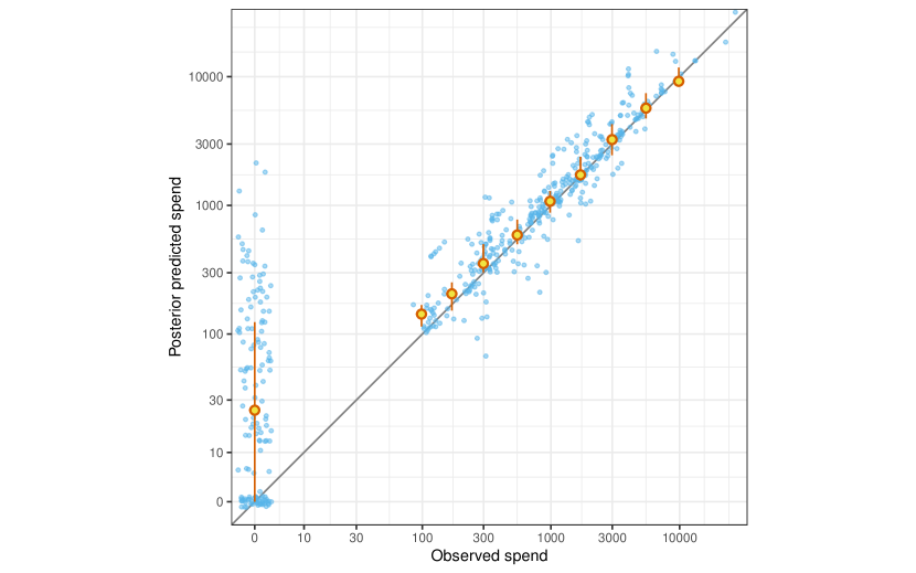
Figure 5: Posterior Predictive Fit for Advertising Spend. Expected total spend for all advertiser-site pairs shown with binned medians and inner 50th percentiles. Points corresponding with advertiser-site pairs with zero observed spend are jittered.

4.2 Parameter Estimates

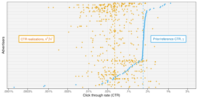
Figure 6: Realized and Prior/Reference Click Through Rates. Each row represents an advertiser and shows the posterior mean of $\gamma_{a}$ and their observed CTRs for sites at which they placed ads. The median CTR is .045%, and the median prior/reference CTR is .232%; both are depicted as vertical dashed lines.

Recall, the key parameter estimates pertain to the advertisers’ prior beliefs about CTRs, and whether they are optimistic or pessimistic. Given that Section 2.2 shows that the number of sites used by advertisers tends to decrease over time and that they tend to switch away from those initial choices, we hazard that advertisers in general tend to be over-optimistic about site match. Hence, the parameter $\gamma_{a}$, which reflects prior beliefs about match (in terms of CTR), should reflect this (see Section 3.2.2). Estimates indicate that for nearly all advertisers, the $\gamma_{a}$s are higher than the empirical CTRs. Figure 6 plots the estimates for $\gamma_{a}$ against the realized click through rates across all observed advertiser-site pairs. Note that the median prior belief for click through rates is .232% while the median true click through rate is about one fifth that amount, .045%. This suggests that advertisers are over-optimistic. There is considerable heterogeneity in initial beliefs, as well as in how accurate those beliefs are, as some are correct, some are optimistic, and some are pessimistic. This result suggests the potential to improve advertiser outcomes by improving prior expectations and reallocating spend across sites.

Figure 7 depicts the changes in advertiser CTR beliefs over time, scaled by the prior belief ($\tilde{c}_{as}/\gamma_{a}$). With no information (that is, in the initial period), this ratio is equal to one. With more information, the ratio approaches $c_{as}/\gamma_{a}$. For example, if the true CTR is twice the initial belief, then this ratio will approach two. Values greater (less) than one imply advertisers are initially pessimistic (optimistic).

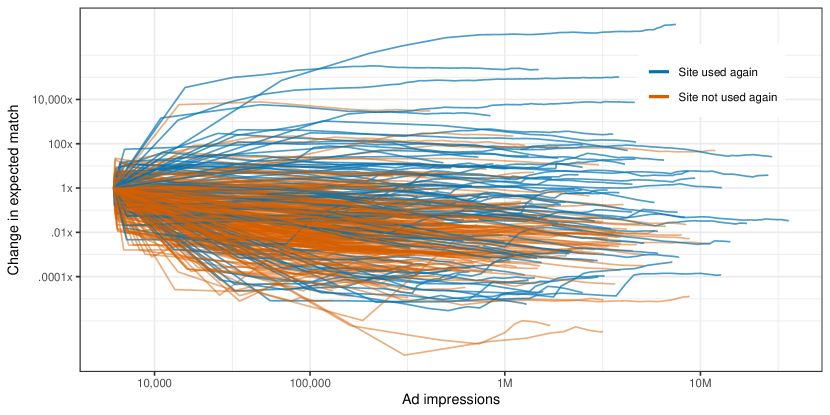
Figure 7: Advertiser Match Beliefs Over Time. Depicts outcomes for the estimation sample, with each line representing an advertiser-site combination. Change in expected match is the ratio of an advertiser’s CTR beliefs to their initial prior, $\tilde{c}_{as}/\gamma_{a}$, which updates based on impressions and clicks observed each day. The horizontal axis presents the cumulative number of impressions (rather than time) to allow comparison across advertiser-site pairs, which differ in impressions served per day and the timing of ad purchases.

Because most of the belief paths decrease from their starting point of 1, we conclude that advertisers are overly optimistic about the likelihood of clicks they will obtain on a site when they first advertise. Moreover, beliefs take several thousand impressions before they begin to stabilize meaning an advertiser could misspend a considerable sum on advertising before learning its true match. Accordingly, advertisers often spend too much, and sometimes spend too little. In each instance, advertisers’ best advertising choices, conditional on them knowing their true match with each site, differ from their actual advertising choices, meaning advertisers face losses relative to if they were fully informed.

Interestingly, one might expect that publishers and the platform have little incentive to address over-optimistic advertisers. If we were to correct advertisers’ prior beliefs about their match with the sites they advertised at, we would expect lower ad spend at those sites, and thus less revenue for those sites and the platform as a whole. However it is also possible that an advertiser could switch to a better matched publisher, potentially increasing total advertising on the publisher sites and the platform owing to better matching. In the next section, we quantify these trade-offs and potential solutions that can benefit advertisers, sites, and the platform.

5 The Role of Information Provision on Advertiser and Publisher Welfare

The results in Section 4 indicate that some advertisers are over-optimistic about advertising efficacy and therefore tend to overspend. Holding all else fixed, redressing this overoptimism concern could cause advertisers to be better off, but publishers to be worse off. On the other hand, advertisers could migrate to other sites that are a better match, increasing their welfare and spend, and thus increasing publisher and network revenue as a result of better sorting. Hence, whether endowing advertisers with better information increases or reduces overall welfare is an empirical question. In this section, we explore how informing advertiser priors, $\tilde{c}_{as}$, affects advertisers’ valuations and spending levels, and explore the consequences for publisher and platform welfare. We begin by outlining approaches to affording better advertiser priors and then consider the welfare implications of these approaches.

5.1 Information Provision

We consider two mechanisms for counterfactual information provision: i) whether or not the advertiser is endowed with full information about the clicks they obtain from their chosen sites, and ii) whether or not advertisers have access to pooled data from other advertisers. We simulate advertising choices and compare advertising spend under each of these mechanisms to a common baseline. Appendix A describes the procedure used to simulate counterfactual data in the baseline and other scenarios.

5.1.1 Simulation Procedure and Baseline Scenario

The baseline and counterfactual scenarios differ in terms of i) the advertisers’ initial information about their expected CTRs, and thus expected match utilities, in week 1; and ii) the advertisers’ choice set, which in turn affects the information available to us when simulating clicks.

Advertisers’ initial information.

In the baseline scenario, $B$, advertisers have the same initial information as in the estimation sample. Thus, for sites at which the advertiser placed ads prior to week 1, their initial expected ratio of CTR to $\gamma_{a}$ in the baseline scenario is $\mathbb{E}[\tilde{c}_{as0}/\gamma_{a}|n_{as0}^{I},n_{as0}^{C},\gamma_{a}]=(1+n_{as0}^{C})/(1+\gamma_{a}n_{as0}^{I})$, with $n_{as0}^{I}>0$—for all other sites, $\mathbb{E}\left[\tilde{c}_{as0}/\gamma_{a}|\gamma_{a}\right]=1$. In the counterfactual scenarios, we augment these initial information states with additional CTR information.

Advertisers’ choice sets.

In the baseline scenario, advertisers’ choice sets are restricted to the sites with observed purchases in the estimation sample, as this allow us to simulate clicks using an approximation to $c_{as}$ based on all advertising outcomes in the full data set. In the counterfactual simulations, we use these approximate values of $c_{as}$ to simulate clicks whenever they are available from the observed advertising data. In some counterfactual scenarios, we expand the advertisers’ choice sets to include all sites in the estimation sample, and accordingly simulate clicks for these sites using an imputed value of $c_{as}$, the procedure for which we describe in Section 5.1.3.

5.1.2 Full Information Within Advertiser

The first counterfactual scenario we consider endows advertisers with full information about the sites for which we observe ad buys in the data. We call this the “full information” counterfactual and denote it $C_{F}$. In this counterfactual scenario, we set $n_{as0}^{I}=10^{12}$ and $n_{as0}^{C}=\left\lfloor 10^{12}c_{as}\right\rfloor$, so that $\mathbb{E}[\tilde{c}_{as0}/\gamma_{a}|n_{as0}^{I},n_{as0}^{C},\gamma_{a},C_{F}]\approx c_{as}/\gamma_{a}$. The value of $c_{as}$ is the same approximate value used in the baseline scenario, and advertisers’ choice sets are restricted to observed advertiser-site pairs, as in the baseline. Hence the only difference between $C_{F}$ and $B$ lies in advertisers’ prior information. This counterfactual yields advertiser spending and revenue as if the advertiser had already known the response they would eventually receive from ads placed on the site (i.e., an oracle prior).

While this counterfactual can yield insights into the advertisers’ losses in the baseline scenario, relative to a hypothetical situation in which they were endowed with complete information about advertising responses at their chosen sites, it does not consider how advertiser outcomes might change at sites where no spending occurred. As noted previously, this limitation is a consequence of only observing CTRs for sites that advertisers actually used in the data. Moreover, this approach to providing advertisers with better information is infeasible because full information about site match is not revealed until after sites are chosen. By then, it is too late for advertisers to change course. Hence, we consider an alternative that involves sharing information across advertisers.

5.1.3 Pooling Information Across Advertisers

Consider a full service ad agency that buys ads on behalf of advertisers (or alternatively, a collective owned by advertisers that acts as a general repository for advertising outcomes). Such an agency can pool information across advertisers and use its experience to forecast which publishers have the highest match with a given advertiser, prior to that advertiser placing any ads. Arguably, a key role of an agency is knowing which types of sites have worked in the past for which types of clients, and one of the reasons advertisers use agencies is to ensure they purchase the correct media to reach the most appropriate audiences. In this counterfactual scenario, therefore, we update advertisers’ prior information by considering the performance of similar advertisers and ads, and extrapolating this information to sites that advertisers did not purchase from in the data. Reflecting advertisers’ augmented information states, we also expand their choice sets to allow ad purchases at any site. When simulating clicks, we use the observed CTRs when available, and the predicted CTRs otherwise. Hence, for sites with observed purchases, there is a discrepancy between advertisers’ expectations, which are based on predicted CTRs, and realizations of clicks, which are based on observed CTRs.

For the purposes of this counterfactual simulation, we assume that ads with similar content generate similar CTRs when placed with a given publisher. More conceptually, we expect that advertisers with similar ads will have similar match with sites’ audiences, and thus generate similar signals about match in terms of CTR. Although our simulation borrows observed CTRs from future outcomes in the data, we consider this an approximation to the knowledge the agency would have accumulated based on past experiences managing campaigns for similar advertisers. We therefore argue that the inferences from this scenario depend on information that is readily available to agencies, and our solution can be practicable to implement.

Estimating advertiser similarities.

In terms of the simulation, our approach entails i) deriving a measure of the similarity between any two advertisers, and ii) pooling outcomes among similar advertisers to predict ad performance. This raises the practical question of how to measure similarity between advertisers for the purpose of our simulations. As is common on many ad platforms, we have no advertiser demographic information in the data. However, in addition to recording the number of impressions and clicks, the platform also retains the images used by advertisers in their display ad campaigns, and these images contain useful information about the advertisers.

To estimate similarity between advertisers, we first retrieve a set of tags describing the content of each display ad placed by advertisers at sites in the focal cluster of 165 liberal blogs. Based on those tags, we construct a term frequency/inverse document frequency (TF-IDF) matrix reflecting how important each tag is in characterizing advertisers. Next, we compute the cosine similarity between advertisers using the TF-IDF measures, producing a square matrix whose cells reflect the pairwise similarity between advertisers. Finally, we use the similarities within each row of this matrix to predict click through rates at all sites in the estimation sample, including in cases where an advertiser did not previously place ads. Appendix B details these specific steps.

Predicting CTRs.

Given a vector of similarities, $r_{a}$, between advertiser $a$ and all other advertisers, as well as the set of advertisers, $\mathcal{A}_{s}$, for which we can approximate $c_{as}$ for site $s$, we predict advertiser $a$’s CTR at site $s$ as

$$\bar{c}_{as}=\frac{\sum_{j\in\mathcal{A}_{s}\backslash a}r_{aj}c_{js}}{\sum_{j\in\mathcal{A}_{s}\backslash a}r_{aj}}.$$ (13)

In this counterfactual scenario, which we refer to as “pooling” and denote $C_{P}$, we set $n_{as0}^{I}=10^{12}$ and $n_{as0}^{C}=\left\lfloor 10^{12}\bar{c}_{as}\right\rfloor$, so that $\mathbb{E}[\tilde{c}_{as0}/\gamma_{a}|n_{as0}^{I},n_{as0}^{C},\gamma_{a},C_{P}]\approx\bar{c}_{as}/\gamma_{a}$.

For advertiser-site pairs with observed ad buys, we can compare the predicted CTRs, $\bar{c}_{as}$, with the observed CTRs, $c_{as}$. Figure 8 shows this comparison by grouping predicted CTRs into bins of roughly equal size and plotting the average observed CTRs corresponding with these predictions. The observations in the plots largely hew to a 45 degree line, meaning that the information can be used from like advertisers to forecast initial click through rates.

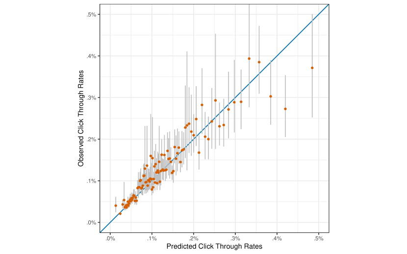
Figure 8: Click Through Rate Predictions. The horizontal axis groups observed imputed click through rates for advertiser publisher pairs into bins of equal numbers of observations, and is truncated above the 99th percentile. The vertical axis corresponds to the actual click through rates for each of these bins. The orange points represent the mean observed click through rate for each binned grouping of imputed click through rates, and the vertical grey bars report bootstrapped 95% CIs for the means. The diagonal line is the 45 degree line. Observations closest to this line are more accurate predictions.

5.1.4 Full Information Combined with Pooling

We also consider a third counterfactual that combines $C_{F}$ and $C_{P}$. In this scenario, advertisers are endowed with full information about their CTRs at sites with observed purchases, as in $C_{F}$, as well as predicted CTRs at all other sites, as in $C_{P}$. We refer to this as the “combined” scenario and denote it $C_{F+P}$. Comparing $C_{F+P}$ to $C_{P}$ provides information about the value of better match information (i.e., oracle versus approximate information about CTRs). Comparing $C_{F+P}$ to $C_{F}$ provides information about the value of expanding advertisers’ choice sets.

5.1.5 Combining Information Within and Across Advertisers

		Own Information
		No Information	Full Information
Shared Information	No Sharing	$B$	$C_{F}$
	Pooled Information	$C_{P}$	$C_{F+P}$

Table 3: Counterfactual Scenarios. The full information condition replaces the first periods’ advertiser CTR priors with the last periods’ oracle CTR posteriors. The shared information condition replaces the first period advertisers’ CTR priors with a similarity weighted average of other advertisers’ CTRs.

Integrating the respective approaches outlined in Sections 5.1.2 and 5.1.3 implies a fully crossed two-by-two counterfactual design as indicated in Table 3. Cell $B$ represents the base case wherein the advertiser has no additional information about other sites or its impending clicks. In the no sharing cells ($B$ and $C_{F})$, advertisers are constrained to choose only the sites upon which they advertised. Cell $B$ involves naïve priors and uses observed CTRs to simulate clicks. Cell $B$ serves as the base case against which we measure the welfare gains from information. Cell $C_{F}$ affords advertisers ex-ante full information on the clicks they obtained ex-post after advertising, erasing their lack of information. Contrasting $C_{F}$ with $C_{B}$ yields theoretical insights into the cost advertisers bear owing to their lack of knowledge on the sites on which they advertised.

Cell $C_{P}$ pools advertiser information using the approach outlined in Section 5.1.3. Contrasting cell $C_{P}$ to $B$ yields the advertiser value of pooling information via an agency or other pooling entity, and expanding the advertisers’ choice set to sites they might otherwise not have considered. Finally, cell $C_{F+P}$ relative to $B$ contrasts having information both from other advertisers (via pooling) and within advertiser (via full information). Other comparisons exist. For example, contrasting differences in $C_{P}$ and $B$ with differences in $C_{F}$ and $B$ yields a sense of which information sets generate greater improvements in advertiser outcomes.

5.2 Advertiser Welfare

		Own Information
		No Information		Full Information
		Spend	Valuations	Spend	Valuations
Shared Information	No Sharing	$0	$0	$-$$180 ($-$22.1%)	$901 (3.5%)
	Pooled	$671 (52.8%)	$2,756 (15.5%)	$546 (45.0%)	$2,984 (16.6%)

Table 4: Advertiser Counterfactual Spending and Revenue Outcomes. Each cell reports the change in the advertisers’ median counterfactual outcome relative to baseline for ad spending and valuations, with the associated percentage increase reported in parentheses.

Table 4 reports the results of the advertiser counterfactual outcomes in terms of relative gains compared to the baseline. Advertiser outcomes are computed using two metrics; change in ad spend and change in valuations. Figure 9 reports the average counterfactual change relative to baseline for each metric in each counterfactual cell in Table 3. Beginning with the full information comparison ($C_{F}$ vs $B$), we find the median ad spend decreases by $180 (22.1%). The preponderance of advertiser priors tend to be updated negatively across the selected sites (i.e., sites with advertising in the data), hence advertisers spend less or stop spending at these sites. As advertisers’ entire ad budgets can be shifted away from the lower match publishers in the set they ultimately selected, the median valuation increases by $901 (3.5%).

Considering next the implications of pooled information ($C_{P}$ vs $B$), we observe a $671 (52.8%) counterfactual increase in median spend. Unlike the $C_{F}$ case, advertisers can shift spend to any publisher, not just amongst those they had used in the baseline case. Hence pooling information enables advertisers to find better matches with new publishers, leading to an increase in ad spending in $C_{F}$ compared to $B$. Advertiser value increases an average of $2,756 (15.5%). The final case, $C_{F+P}$, combines both within-advertiser oracle and pooled information. The combined case’s results largely hew to the pooled information counterfactual because the oracle priors only apply to a limited number of sites. Hence, the solutions across $C_{F+P}$ and $C_{P}$ are similar. The median advertising spend increases $546 (45.0%) and the median advertiser welfare increases $2,984 (16.6%). As the information requirements from the $C_{P}$ case is closest to what could be implemented in practice, our subsequent discussion focuses upon the pooled information scenario, $C_{P}$.

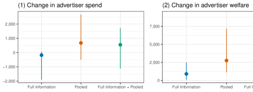
Figure 9: Counterfactual Advertiser Welfare. Panel (1) presents the posterior mean (represented by a point) and 95% CI (represented by a bar) change in ad spend relative to baseline across the three counterfactual conditions. Panel (2) reports the posterior mean and 95% CI for change in advertiser valuations (welfare).

Decomposing spend across advertisers in the pooling counterfactual, $C_{P}$, Figure 10 reports the change in spend (along the horizontal axis) for each of the 100 advertisers (along the vertical axis), where advertisers are sorted from most negative expected change in spend to most positive. The figure suggests considerable heterogeneity in spending changes, presumably owing to considerable difference across advertisers in both information states and match values. Advertisers with higher levels of spending tend to show the greatest counterfactual change in absolute levels of spend, presumably owing to their larger ad budgets to reallocate.

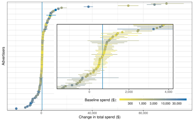
Figure 10: Change in Spend by Advertiser Under the Pooling Counterfactual. Inset shows the inner 60% of advertisers at higher resolution. Points indicate posterior means, horizontal bars are bootstrap 95% CIs for the means. Vertical line indicates the median outcome.

Figure 11 depicts the change in the number of publishers used by advertisers under the pooling counterfactual, $C_{P}$. If the high and incorrect priors dominate, then most advertisers will decrease the number of publishers used. If the assortive matching effect dominates, then advertisers will sort into more sites. In this regard, the four quadrants of the figure represent the degree to which advertisers added new publishers to their set of advertising options, deleted them, continued to use them under the counterfactual setting, or never used them in either the baseline or counterfactual setting. In the lower right quadrant (panel 4), we observe that most sites not chosen by advertisers under $B$ continue not to be chosen under $C_{P}$. For example, twenty of the 100 advertisers did not use 18 of the 20 publishers in both the baseline and counterfactual setting. Comparing the histogram in the upper left cell (panel 1) to the one in the upper right (panel 2), we note that more new publishers were added by advertisers than removed as advertisers found good matches, and that pooling information induces considerable change in advertiser behavior. Overall, this figure suggests that, rather than concentrating on a single publisher or merely eliminating sites where prior beliefs were too high, advertisers seem to be sorting into better matches (that is, finding sites that generate higher advertising value).

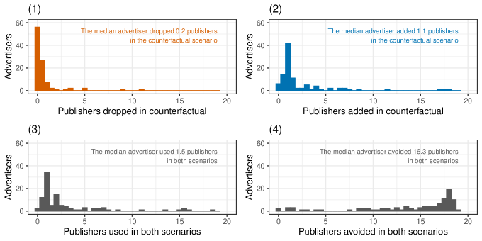
Figure 11: Change in Publisher Usage by Advertisers Under the Pooling Counterfactual. Each vertical bar represents the number of advertisers that evidenced a given level change in publisher usage across the baseline and counterfactual condition. For example, the first bar in panel (1) indicates that nearly 60 advertisers dropped no publishers in the counterfactual. The third bar in panel (1) indicates that over 40 advertisers dropped one publisher.

5.3 Publisher and Platform Welfare

Table 5 reports and Figure 12 depicts how revenues change across the 20 publishers under pooled information. The network collects a flat percentage of publisher revenues, thus these changes are proportional to the network’s gains and losses.

		Own Information
		No Information	Full Information
Shared Information	No Sharing	$0	$-$$4,684 ($-$21.0%)
	Pooled Information	$9,618 (63.9%)	$8,879 (46.3%)

Table 5: Publisher Counterfactual Revenue Outcomes

Two effects of information provision, that is, endowing advertisers with better priors, are possible. First, as advertisers are generally over-optimistic regarding the sites they had historically chosen, demand at publisher sites could decrease and revenues could fall. Alternatively, as suggested by Figure 12, advertisers can better sort into a match across publisher sites, finding new options that generate greater value than that from the set of publishers selected in the baseline setting. Comparing $C_{F}$ to $B$, we find that 18 of the 20 publishers lose revenue and that the median revenue loss is $4,684 (21.0%), because the optimistic advertiser prior effect dominates. Advertisers realize that they were too optimistic, but are not provided information about better potential matches, so they cut spending. In such a scenario, it is likely that the network and publishers would seek to not inform advertisers that their priors were too high, as the network and publisher sites would lose money. However, comparing $C_{P}$ to $B,$ we find that all publishers gain revenue, with a median increase of $9,618 (63.9%). The revenue from $C_{F+P}$ is lower than $C_{P}$ because the negative effect on spending from correcting advertisers’ optimistic priors offsets the effects of better matching to some degree, though the latter effect dominates. Overall, the sorting effect dominates the prior effect, and the pooled information agency mechanism generates not only positive welfare outcomes for advertisers, but also for publishers.

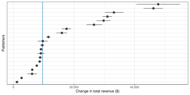
Figure 12: Change in Publisher Revenue by Site Under the Pooling Counterfactual. Points indicate posterior means, horizontal bars are bootstrap 95% CIs for the means. Publishers are sorted along the ordinate from lowest to highest change in mean revenue. Vertical line indicates the median outcome.

Focusing again on the pooling counterfactual, $C_{P}$, we see that not only do publishers gain revenue, but they also tend to serve more advertisers. Figure 13 reports the distribution (across publishers) of the number of advertisers lost (left panel) and gained (right panel) in $C_{P}$ versus $B$. Comparing the two distributions. it is evident that more advertisers are gained than lost, consistent with the view that the effects of enhancing match by enabling advertisers to find higher value publishers more than offsets the loss of advertisers who had over-optimistic priors.

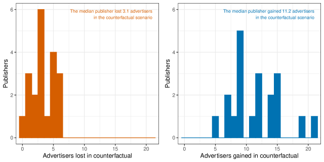
Figure 13: Distribution of Advertisers Gained and Lost by Publishers Under the Pooling Counterfactual. Each vertical bar represents the number of publishers that evidenced a given level change in advertisers across the baseline and counterfactual condition. For example, the first bar in the left hand panel indicates that one publisher lost no advertisers. The second bar indicates that 3 publishers lost two advertisers.

5.4 Counterfactual Summary

Based on the median publisher gain of $2,756 and the median advertiser gain of $671, we find that the combined welfare gains across the 100 advertisers and 20 publishers over the six month window over our estimation data is on the order of $122,220 under the pooling counterfactual. To the extent one can extrapolate the gains across the entire ad network’s 8000 advertisers and 3200 publishers, total welfare gains would be as much as $14 million. This extrapolation is likely optimistic because our sample is weighted to larger publishers and blogs, but suspect the potential welfare gains remain considerable even when the total is scaled downward to reflect the smaller advertiser and publisher sizes. Yet the calculation is suggestive of the value of sharing information. To the extent a similar pooled approach could be used across multiple ad networks or other ad channels such as retail media, gains would be much larger.

As a caveat, it should be noted that our counterfactual analysis constitutes a partial equilibrium. Publisher sites, faced with increased demand could raise subscription prices. To the extent this occurs, advertiser gains will be somewhat diminished and publisher gains should be somewhat decreased. However, we note most gains come from sorting. As suggested by figure 13, sites tend to face a change in advertiser composition owing to better sorting rather than having all advertisers concentrate into a single site. To the extent sites are imperfect substitutes, this lack of concentration should offset the tendency of any dominant site to substantially raise prices. It is further possible that changes in advertising information have downstream consequences for firms’ pricing strategies, that could offset some of their gains by increasing price competition; these issues are beyond the scope of our research.

6 Conclusions

In this paper we consider the implications of advertiser learning in direct display advertising markets. In contrast to exchange markets, advertising is bought in bulk (many thousands of impressions) rather than sequentially, which limits advertisers’ opportunities to use test and learn strategies to efficiently identify publishers whose audiences are a good match for their ads [28]. In direct exchange contexts, advertisers’ initial information states are economically consequential because, lacking the ability to test and learn incrementally, they are effectively guessing which publishers to use. Hence, there is a considerable potential to choose sites incorrectly and, as a corollary, to enhance advertiser (and possibly publisher) welfare by endowing advertisers with better information.

To ascertain whether advertisers have incorrect beliefs and assess the potential consequences thereof, we collect direct sale data from an ad exchange. The data describe ad purchases from the exchange’s inception, providing an ideal setting to explore the nature of advertiser learning as advertisers enter the network. Patterns in these data suggest evidence of advertiser learning. Advertisers initially run ads at relatively many sites and, after additional exploration, ultimately settle on a smaller number where they presumably find greater customer response. Using a direct utility model of advertiser choices of ad subscriptions across sites, in which match is allowed to be learned from past advertising outcomes, we document that advertisers’ initial priors are quite misinformed. They overestimate initial clickthrough rates by a factor of nearly five; the median beliefs are 0.23% and the actual rates are 0.045%. As such, advertisers are initially far too optimistic about the publishers they have chosen for advertising.

Next we consider various mechanisms to redress this problem and ascertain the impact of advertiser information on advertiser welfare and publisher revenues. We consider two such mechanisms. The first uses advertiser outcomes at the end of the data to inform their priors at the start of the data. While this suggests how much advertiser outcomes could potentially improve on the sites they actually explored, the approach cannot inform us about how well advertisers would fare on sites they did not explore. Moreover, the mechanism is impracticable, inasmuch as it is impossible to know ad outcomes ex ante. Hence, we consider a second mechanism wherein advertisers can pool information on ad outcomes and design via an agency by drawing on similar advertisers who previously placed ads on the considered sites. In this scenario, the agency, through its experience, knows which types of sites generate the best match for advertisers. We operationalize this information sharing mechanism using the Google Image API to impute similarity between ads, and then using this similarity information to forecast advertising responses for advertisers encountering new publisher sites (as the similarity weighted combination of outcomes for like ads that have previously appeared on those sites). We find this approach is predictive of advertising performance for new ads on publisher sites.

Endowing advertisers with pooled information leads to a median advertiser increase of 52.8% ($671) in ad spend, and a median advertiser welfare gain of 15.5% ($2,756). On the publisher side, we note two opposing forces; rectifying optimistic priors should decrease ad spend and revenue at sites, while better sorting of match between advertisers and publisher sites should lead to higher revenue. The latter effect dominates, generating a median publisher gain of 63.9% ($9,618). All publishers gain in revenue. In other words, redressing advertiser misinformation in direct ad networks leads to large welfare gains for publishers and advertisers alike. Extrapolating these gains across all 8,000 advertisers and 3,200 publishers in our considered network suggests welfare gains up to $14,000,000 (the total is likely to be somewhat smaller because our analysis focuses on the larger publishers). The information pooling approach, if ported to other direct advertising networks, would yield even greater gains. Of note, direct ad purchasing also exists in non-digital channels as well, such as television, radio, and out of home. It stands to reason that advertisers also face a learning problem in those contexts, but the number of publisher alternatives in digital dwarfs these other channels and likely exacerbates the learning problem and potential gain from redressing it.

Our analysis focuses on the advertiser demand side. An interesting potential extension is to consider publisher ad pricing responses to changes in advertiser demand. To the extent that advertiser demand increases, publishers can raise ad prices and increase their share of total welfare gains at the cost of advertisers. That said, we note that efficient sorting can reduce the concentration of advertisers on some sites and raise it on others making the overall effect ambiguous and highly variable across publishers. Given that publishers face a large competitive set in the face of dynamic demand as a result of learning, the supply side problem would be a challenging but useful extension in the analysis of direct display advertising markets. Another issue of interest is how to balance inventory and pricing across both direct and exchange markets [3], a challenge exacerbated by advertiser learning. In sum, we hope this research sparks more interest on these and other topics in this large and economically consequential direct advertising market.

Appendix A Simulation Procedure

All counterfactual scenarios share a common simulation procedure based on 100 draws from the posterior distribution of the model parameters, $\theta$. For each draw of $\theta$, $\epsilon$ is sampled from the posterior predictive distribution of $\epsilon|\theta$, and the same $\epsilon$ vector is used for each baseline/counterfactual pair (each counterfactual is paired with a unique baseline simulation). If a simulated choice has a corresponding observed choice, then $\epsilon_{asw}$ is truncated by the upper and lower bounds defined in Equations (8) and (9), conditional on $\theta$. We average over draws of $\theta$ to obtain posterior predictive means for the outcomes of interest.

Using the set of available ad durations, $x$, and prices, $p$, from the estimation sample, purchases for advertiser $a$ are simulated starting with week $w=1$ (or the earliest week the advertiser was observed in the network if the advertiser joined during the estimation period). For each site $s$, advertiser $a$ chooses an optimal number of days of advertising, $x$. If $x=0$, advertiser $a$ does not place an ad at site $s$ in week $w$. Otherwise, $x>0$ and we assume $n^{I}=x\cdot t_{s}$ impressions are delivered, yielding $n^{C}\big{|}n^{I},c_{as}\,\sim\mathrm{Binomial}(n^{I},c_{as})$ clicks. If $0\leq x\leq 7$, then the next advertising choice for site $s$ occurs in week $w+1$; otherwise the next choice occurs in a later week, depending on the value of $x$ . The procedure repeats for each site, and then advances to the next week. Choices in subsequent weeks are informed by Bayesian updating on $\tilde{c}_{as}$ based on the cumulative number of impressions, $n^{I}$, and clicks, $n^{C}$, obtained from previous ad buys.

The outcomes of interest from these simulations are i) the amount each advertiser spends in total or at each site, which we obtain directly from the simulations; and ii) a measure of advertiser welfare. Regarding the latter: because advertisers choose sites based on net expected payoff (Equation (1)), expected net payoffs are transformed into a “true” net payoff by replacing the simulated value of $\mathbb{E}\left[\tilde{c}_{asw}|n_{asw}^{I},n_{asw}^{C}\right]$ with $\mathbb{E}\left[\tilde{c}_{asw}|n^{I}=10^{12},n^{C}=\left\lfloor 10^{12}c_{as}\right\rfloor\right]$. We use $\mathbb{E}\left[\tilde{c}_{asw}|n^{I}=10^{12},n^{C}=\left\lfloor 10^{12}c_{as}\right\rfloor\right]$ rather than $c_{asw}$ because the procedure for counterfactually manipulating advertisers’ prior beliefs (explained below) entails altering their state space ($n^{I}$ and $n^{C}$) in a similar manner. Using $c_{asw}$ instead would introduce simulation error due to differences in floating point precision for large numbers.

Appendix B Measuring Advertising Similarity

To tag ad images, we use Google’s Cloud Vision API, a pre-trained machine learning model developed by Google which ingests images as inputs and returns labels as an output. Using this product, we query the set of 10 tags that best characterize each ad image in our dataset. Figure 14 depicts an example ad from the dataset, and Google’s Cloud Vision API retrieves the following tags for this image: television program, television presenter, tie, news, font, display device, event, cable television, electric blue and public speaking.

Figure 14: Example Of An Ad Image In The Dataset.

Using the ad image tags returned by Google API, we construct a TF-IDF matrix of advertisers by tags [23]. When computing similarity, TF-IDF upweights ad tags that are unique and down-weights commonly appearing tags, as distinctive characterizations of an image are most informative.

Figure 15 reports the top 10 TF-IDF tags for the four advertisers appearing most frequently in the data. The most frequent advertiser (Advertiser A) is primarily characterized by tags related to food. Similarly, the third most frequent advertiser (Advertiser C) purveys products related to plants. In this sense, the TF-IDF describes advertisers based on the ads shown in their campaigns.

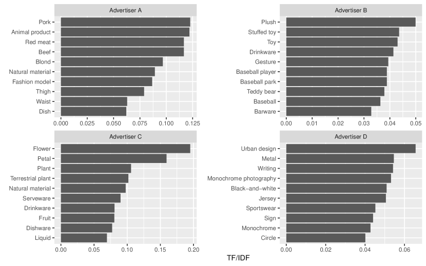
Figure 15: Top 10 Tags For The Top 4 Advertisers. Advertiser A placed the most ads in the data set, Advertiser D the fourth most. Depicts the ten tags with the highest TF-IDF for each advertiser.

To measure the similarity between advertisers based on their ad images tags, we compute the cosine similarity of their TF-IDF vectors. The cosine similarity between two vectors $a$ and $b$ is $f(a,b)=\frac{a\cdot b}{||a||\,||b||}=\frac{\sum_{k}a_{k}b_{k}}{\sqrt{\sum_{k}a_{k}^{2}}\sqrt{\sum_{k}b_{k}^{2}}}$ and ranges from 0 to 1: it is 0 when the ad vectors are orthogonal and 1 when the ad vectors are identical. Stacking the vectors of advertisers’ cosine similarities with other advertisers yields a square and symmetric matrix $R$ with 1 in the main diagonal and entries $r_{aj}$ containing the cosine similarity between advertiser $a$ and advertiser $j$. The ad copy similarity matrix $R$ is then used to generate a weighted prediction of CTRs for advertisers on sites where they have not previously advertised, per Equation (13), under the assumption that similar items have similar click through rates on a site.

References

- [1] Amine Allouah and Omar Besbes “Auctions in the online display advertising chain: A case for independent campaign management” In Columbia Business School Research Paper, 2017
- [2] Susan Athey and Glenn Ellison “Position auctions with consumer search” In The Quarterly Journal of Economics 126.3 Oxford University Press, 2011, pp. 1213–1270
- [3] Santiago R Balseiro, Jon Feldman, Vahab Mirrokni and S Muthukrishnan “Yield optimization of display advertising with ad exchange” In Management Science 60.12 INFORMS, 2014, pp. 2886–2907
- [4] Santiago R Balseiro and Yonatan Gur “Learning in repeated auctions with budgets: Regret minimization and equilibrium” In Management Science 65.9 INFORMS, 2019, pp. 3952–3968
- [5] Santiago R. Balseiro, Omar Besbes and Gabriel Y. Weintraub “Repeated auctions with budgets in ad exchanges: Approximations and design” In Management Science 61.4 INFORMS, 2015, pp. 864–884
- [6] Santiago R. Balseiro and Ozan Candogan “Optimal contracts for intermediaries in online advertising” In Operations Research 65.4, 2017, pp. 878–896
- [7] Chandra R Bhat “The multiple discrete-continuous extreme value (MDCEV) model: Role of utility function parameters, identification considerations, and model extensions” In Transportation Research Part B: Methodological 42.3 Elsevier, 2008, pp. 274–303
- [8] Han Cai, Kan Ren, Weinan Zhang, Kleanthis Malialis, Jun Wang, Yong Yu and Defeng Guo “Real-time bidding by reinforcement learning in display advertising” In Proceedings of the Tenth ACM International Conference on Web Search and Data Mining Cambridge, United Kingdom: Association for Computing Machinery, 2017, pp. 661–670 DOI: 10.1145/3018661.3018702
- [9] Hana Choi, Carl F. Mela, Santiago R. Balseiro and Adam Leary “Online display advertising markets: A literature review and future directions” In Information Systems Research 31.2, 2020, pp. 556–575
- [10] W. Choi and Amin Sayedi “Learning in online advertising” In Marketing Science 38.4, 2019, pp. 584–608
- [11] Jyotirmoy Gope and Sanjay Kumar Jain “A survey on solving cold start problem in recommender systems” In 2017 International Conference on Computing, Communication and Automation (ICCCA), 2017, pp. 133–138 IEEE
- [12] Xuan Nhat Lam, Thuc Vu, Trong Duc Le and Anh Duc Duong “Addressing cold-start problem in recommendation systems” In Proceedings of the 2nd international conference on Ubiquitous information management and communication, 2008, pp. 208–211
- [13] Sanghak Lee and Greg M Allenby “Modeling indivisible demand” In Marketing Science 33.3 INFORMS, 2014, pp. 364–381
- [14] Blerina Lika, Kostas Kolomvatsos and Stathes Hadjiefthymiades “Facing the cold start problem in recommender systems” In Expert systems with applications 41.4 Elsevier, 2014, pp. 2065–2073
- [15] John D.. Little and Leonard M. Lodish “A media planning calculus” In Operations Research 17.1, 1969, pp. 1–35
- [16] Jia Liu and Olivier Toubia “A semantic approach for estimating consumer content preferences from online search queries” In Marketing Science 37.6 INFORMS, 2018, pp. 930–952
- [17] Sridhar Narayanan and Puneet Manchanda “Heterogeneous learning and the targeting of marketing communication for new products” In Marketing Science 28.3, 2009, pp. 424–441
- [18] Claudia Perlich, Brian Dalessandro, Rod Hook, Ori Stitelman, Troy Raeder and Foster Provost “Bid optimizing and inventory scoring in targeted online advertising” In Proceedings of the 18th ACM SIGKDD international conference on knowledge discovery and data mining, 2012, pp. 804–812 ACM
- [19] K. Ren, W. Zhang, K. Chang, Y. Rong, Y. Yu and J. Wang “Bidding machine: Learning to bid for directly pptimizing profits in display advertising” In IEEE Transactions on Knowledge and Data Engineering 30.4, 2018, pp. 645–659 DOI: 10.1109/TKDE.2017.2775228
- [20] Andrew I. Schein, Alexandrin Popescul, Lyle H. Ungar and David M. Pennock “Methods and metrics for cold-start recommendations” In Proceedings of the 25th Annual International ACM SIGIR Conference on Research and Development in Information Retrieval, SIGIR ’02 Tampere, Finland: Association for Computing Machinery, 2002, pp. 253–260 DOI: 10.1145/564376.564421
- [21] Eric M. Schwartz, Eric T. Bradlow and Peter S. Fader “Customer acquisition via display advertising using multi-armed bandit experiments” In Marketing Science 36.4, 2017, pp. 500–522
- [22] Steven L. Scott “A modern Bayesian look at the multi-armed bandit” In Applied Stochastic Models in Business and Industry 26.6, 2010, pp. 639–658
- [23] Julia Silge and David Robinson “tidytext: Text mining and analysis using tidy data principles in R” In Journal of Open Source Software 1.3, 2016, pp. 37
- [24] Daniel Simpson, Håvard Rue, Andrea Riebler, Thiago G. Martins and Sigrunn H. Sørbye “Penalising Model Component Complexity: A Principled, Practical Approach to Constructing Priors” In Statistical Science 32.1 Institute of Mathematical Statistics, 2017 DOI: 10.1214/16-sts576
- [25] Stan Development Team “RStan: the R interface to Stan. R package version 2.16.2”, 2017 URL: http://mc-stan.org
- [26] Steven Tadelis, Christopher Hooton, Utsav Manjeer, Daniel Deisenroth, Nils Wernerfelt, Nick Dadson and Lindsay Greenbaum “Learning, sophistication, and the returns to advertising: Implications for differences in firm performance”, Working Paper Series 31201, 2023 DOI: 10.3386/w31201
- [27] Olivier Toubia and Oded Netzer “Idea generation, creativity, and prototypicality” In Marketing science 36.1 INFORMS, 2017, pp. 1–20
- [28] Srinivas Tunuguntla and Paul R. Hoban “A near-optimal bidding strategy for real-time display advertising auctions” In Journal of Marketing Research 58.1, 2021, pp. 1–21 DOI: 10.1177/0022243720968547
- [29] Hal R Varian “Position auctions” In International Journal of Industrial Organization 25.6 Elsevier, 2007, pp. 1163–1178
- [30] Aki Vehtari, Andrew Gelman and Jonah Gabry “Practical Bayesian model evaluation using leave-one-out cross-validation and WAIC” In Statistics and Computing 27.5 Springer ScienceBusiness Media LLC, 2017, pp. 1413–1432 DOI: 10.1007/s11222-016-9696-4
- [31] Caio Waisman, Harikesh S. Nair and Carlos Carrion “Online causal inference for advertising in real-time bidding auctions” arXiv, 2019 DOI: 10.48550/ARXIV.1908.08600
- [32] Chunhua Wu “Matching value and market design in online advertising networks: An empirical analysis” In Marketing Science 34.6, 2015, pp. 906–921
- [33] Boya Xu, Yiting Deng and Carl Mela “A scalable recommendation engine for new users and items” arXiv, 2022 DOI: 10.48550/ARXIV.2209.06128
- [34] Zijun Yao, Deguang Kong, Miao Lu, Xiao Bai, Jian Yang and Hui Xiong “Multi-view multi-task campaign embedding for cold-start conversion rate forecasting” In IEEE Transactions on Big Data 9.1, 2023, pp. 280–293 DOI: 10.1109/TBDATA.2022.3162150