Generalizing Thiele Equation

Abstract

We generalize the Thiele equation with a transverse velocity to the skyrmion motion described by the collective coordinate of magnetization vector. It is applied to investigate significant disparity in the existing data sets of skyrmion and antiskyrmion Hall angles. Our analysis further reveals interesting differences of these Hall angles near the angular momentum compensation point. We identify a possible physical quantity that is responsible for the disparity.

Thiele Thiele described the steady state motion of domain wall or skyrmion by parameterizing the unit magnetization vector $\vec{n}$ as

$$n_{i}=M_{i}(x_{j}-X_{j})/M_{s}\;,$$ (1)

where $M_{s}=|\vec{M}|$ is a saturation magnetization, and $x_{i}$ the field position. Roman indices $i,j$ represent the spatial vector components with repeated ones summed over. The collective coordinate $X_{j}$ is parametrized as

$$X_{i}=v_{i}t$$ (2)

to describe the center of domain wall or skyrmion, which moves with a velocity $v_{i}$ as time $t$ ticks.

The resulting Thiele equation has the form

$$\mathcal{G}_{ij}v_{j}+\alpha\mathcal{D}_{ij}v_{j}+F_{i}=0\;,$$ (3)

where $\alpha$ is a damping parameter, and

$$\begin{split}\mathcal{G}_{ij}&=\frac{M_{s}}{\gamma_{0}}\epsilon_{lmn}\large\int d^{2}x~{}n_{l}(\partial_{i}n_{m})(\partial_{j}n_{n})\;,\\ \mathcal{D}_{ij}&=-\frac{M_{s}}{\gamma_{0}}\large\int d^{2}x~{}(\partial_{i}n_{k})(\partial_{j}n_{k})\;,\\ F_{i}&=-M_{s}\int d^{2}x(\partial_{i}n_{j})H_{\text{eff},j}\;.\end{split}$$ (4)

Here $\gamma_{0}$ is gyromagnetic ratio, $\mathcal{G}_{ij}v_{j}$ is the Magnus force, $\mathcal{D}_{ij}v_{j}$ is total dissipative drag force, and $F_{i}$ is total external force that includes forces due to effective magnetic field and various spin torques. Internal forces due to anisotropy and exchange energies, internal demagnetizing fields, magnetostriction do not contribute Thiele .

Since its publication on 1973, the Thiele equation has been extensively used to describe the steady state motion of magnetic structures such as domain walls or skyrmions. Note that the Magnus force is proportional to the skyrmion charge $Q$, $\mathcal{G}_{ij}\propto\epsilon_{ij}Q=\epsilon_{ij}\large\int d^{2}x~{}\epsilon_{lmn}n_{l}(\partial_{x}n_{m})(\partial_{y}n_{n})$ in a 2 dimensional film geometry with coordinates $(x,y)$.

Here we propose to generalize the Thiele equation (3) with an additional transverse velocity in addition to $v_{i}$ of the collective coordinate as Kim:2020piv

$$X_{i}=v_{i}t+R\epsilon_{ij}v_{j}t\;,$$ (5)

where the parameter $R$ represents the strength of the transverse velocity compared to the original one. This generalization has been introduced in Kim:2020piv . Here we further examine its consequences near the angular momentum compensation point in the context of ferrimagnets.

The Thiele equation can be derived from the Landau-Lifshitz-Gilbert (LLG) equation LandauFluidMechanics GilbertEq

$$\partial_{t}\vec{M}=-\gamma_{0}\vec{M}\times\vec{H}_{\text{eff}}+\frac{\alpha}{M_{s}}\vec{M}\times\partial_{t}\vec{M}\;.$$ (6)

As $M_{i}$ and $\partial_{t}M_{i}$ are orthogonal to each other (due to the normalized magnetization vector, $\vec{n}^{2}=1$), one can show the equation

$$-\frac{\epsilon_{jkl}M_{k}\partial_{t}M_{l}}{\gamma_{0}M_{s}^{2}}-\alpha\frac{\partial_{t}M_{j}}{\gamma_{0}M_{s}}+\tilde{\beta}M_{j}+H_{\text{eff},j}=0$$ (7)

is equivalent to the LLG equation. Explicitly, it can be checked by multiplying $-\epsilon_{jik}M_{k}$ to (7), summing over $j$, and renaming the indices. The third term in (7) does not contribute below as its coefficient is fixed as $\tilde{\beta}=-M_{j}H_{j}/M_{s}^{2}$ that can be verified by multiplying $M_{j}$ to (7).

Thiele equation has been used recently, for example, to compute the velocity of various topological spin structures such as ferromagnetic skyrmion-based logic gates and diodes ThieleEQAdded1 , antiferromagnetic skyrmion-based oscillators ThieleEQAdded2 and antiferromagnetic bimerons ThieleEQAdded3 .

To derive the Thiele equation with the generalization (5), we multiply $-\partial M_{j}/\partial x_{i}$ to (7). The third term drops out as $M_{j}\partial_{i}M_{j}=0$. Note the time derivative $\partial_{t}\vec{M}$ has an additional contribution due to the second term in (5).

$$\partial_{t}M_{i}=(v_{j}+R\epsilon_{jk}v_{k})\partial_{j}M_{i}\;.$$ (8)

By integrating over a (skyrmion) volume, one arrives at

$$\mathcal{G}_{ij}(v_{j}+R\epsilon_{jk}v_{k})+\alpha\mathcal{D}_{ij}(v_{j}+R\epsilon_{jk}v_{k})+F_{i}=0\;.$$ (9)

Two coefficients $\mathcal{G}_{ij},\mathcal{D}_{ij}$ and the force term $F_{i}$ are given in (4). This is the Thiele equation generalized with the transverse velocity. Hereafter, we use the same notations of (9) after multiplying $\gamma_{0}/M_{s}$, for example, $(\gamma_{0}/M_{s})F_{i}\to F_{i}$.

It is interesting to see some general features of the new contributions. First, $\mathcal{G}_{ij}=G\epsilon_{ij}$, antisymmetric with the two indices $ij$. Thus

$$\mathcal{G}_{ij}(v_{j}+R\epsilon_{jk}v_{k})=G\epsilon_{ij}v_{j}-GRv_{i}\;.$$ (10)

Thus the new term $\mathcal{G}_{ij}R\epsilon_{jk}v_{k}$ actually increase or decrease the longitudinal velocity $v_{i}$ depending on the sign of $GR$, while the original term $\mathcal{G}_{ij}v_{j}$ is transverse to $v_{j}$ that is the Magnus force.

Second, we decompose the drag tensor into symmetric and antisymmetric parts as $\mathcal{D}_{ij}=D_{s}\delta_{ij}+D_{a}\epsilon_{ij}$. The symmetric part gives

$$\alpha D_{s}v_{i}+\alpha D_{s}R\epsilon_{ik}v_{k}\;.$$ (11)

The new contribution $\alpha D_{s}R\epsilon_{ik}v_{k}$ modifies the transverse motion added to the contribution $G\epsilon_{ij}v_{j}$, while $\alpha D_{s}v_{i}$ is the contribution Thiele derived.

On the other hand, the antisymmetric part is given by

$$\alpha D_{a}\epsilon_{ij}v_{j}-\alpha D_{a}Rv_{i}\;.$$ (12)

This has the same structures of the first term in (9). Thus these can be combined as $G\to G+\alpha D_{a}$. Then our result (9) can be recast as

$$\begin{split}&\big{[}\alpha D_{s}-(G+\alpha D_{a})R\big{]}v_{i}\\ &+\big{[}(G+\alpha D_{a})+\alpha D_{s}R\big{]}\epsilon_{ij}v_{j}+F_{i}=0\;.\end{split}$$ (13)

Thus we see that both the original longitudinal and transverse velocity components are modified by $R$.

Using this form (13) in 2 dimensions $(x,y)$, it is straightforward to compute the Hall angle. Without loss of generality, we set the force along the $x$ coordinate. Then the equation along $y$ direction gives $[\alpha D_{s}-(G+\alpha D_{a})R]v_{y}=[(G+\alpha D_{a})+\alpha D_{s}R]v_{x}$. Then the Hall angle is given by

$$\begin{split}&\tan\theta_{H}=\frac{v_{y}}{v_{x}}=\frac{(G+\alpha D_{a})+\alpha D_{s}R}{\alpha D_{s}-(G+\alpha D_{a})R}\;.\end{split}$$ (14)

This is our generalization of the Hall angle in the presence of the new transverse effect (5). It does not depend on details of the external force. Note that this Hall angle depends on the parameter $R$ in two different ways, which are related to the transverse contribution $\alpha D_{s}R\epsilon_{ik}v_{k}$ and the longitudinal ones $-(G+\alpha D_{a})Rv_{i}$. A simpler version of (14) appeared previously in KimBook Kim:2020piv .

Without the new transverse effect ($R=0$), the Hall angle (14) reduces to

$$\begin{split}&\tan\theta_{H}=\frac{v_{y}}{v_{x}}=\frac{G+\alpha D_{a}}{\alpha D_{s}}\;.\end{split}$$ (15)

We further checked $D_{a}=0$ for the stable positive- and negative-charge skyrmions with $Q=\pm 4\pi$ Jiang2017 . Thus their Hall angles are the same with opposite signs.

We note that our convention for skyrmion topological charge has an additional $4\pi$ footnoteSkyrmionCharge compared to the definition given in SKCharge . There are related confusions in literature Han as mentioned in footnoteSkyrmionCharge .

After describing continuous skyrmion model, we look into basic aspects of the generalized Thiele equation (9) and investigate the positive- and negative-charge skyrmion Hall angles using (14).

Continuous skyrmion model
The constraint $\vec{n}^{2}=1$ allows us to parametrize the vector $\vec{n}=\sin\Theta\cos\Phi\hat{\rho}+\sin\Theta\sin\Phi\hat{\phi}+\cos\Theta\hat{z}$ with two dimensional coordinates $(\rho=(x^{2}+y^{2})^{-1/2},\phi=\tan^{-1}(y/x))$ and its perpendicular direction $z$. An isolated Néel-type skyrmion has $\Phi=0$ and thus can be modeled as Jiang2017

$$\vec{n} =\sin\Theta(\rho)\hat{\rho}+\cos\Theta(\rho)\hat{z}\;,$$ (16)

with a parametrization

$$\Theta(\rho)=\left\{\begin{matrix}\pi\;,&\quad\;&\rho-P<-\omega\;\\ \vspace{-0.1in}&&\\ \frac{1}{2}\pi-\frac{\rho-P}{2\omega}\pi\;,&&-\omega\leq\rho-P\leq\omega\;,\\ \vspace{-0.1in}&&\\ 0\;,&&\rho-P>\omega\;\end{matrix}\right.$$ (17)

where $P$ and $2\omega$ represent the position and width of the domain wall (DW) illustrated in Fig. 1. This DW describes the interpolating region of the negative-charge skyrmion with spin up $\vec{n}=\hat{z}$ in the outer region $\rho>P+\omega$ and with spin down $\vec{n}=-\hat{z}$ in the inner region $\rho<P-\omega$.

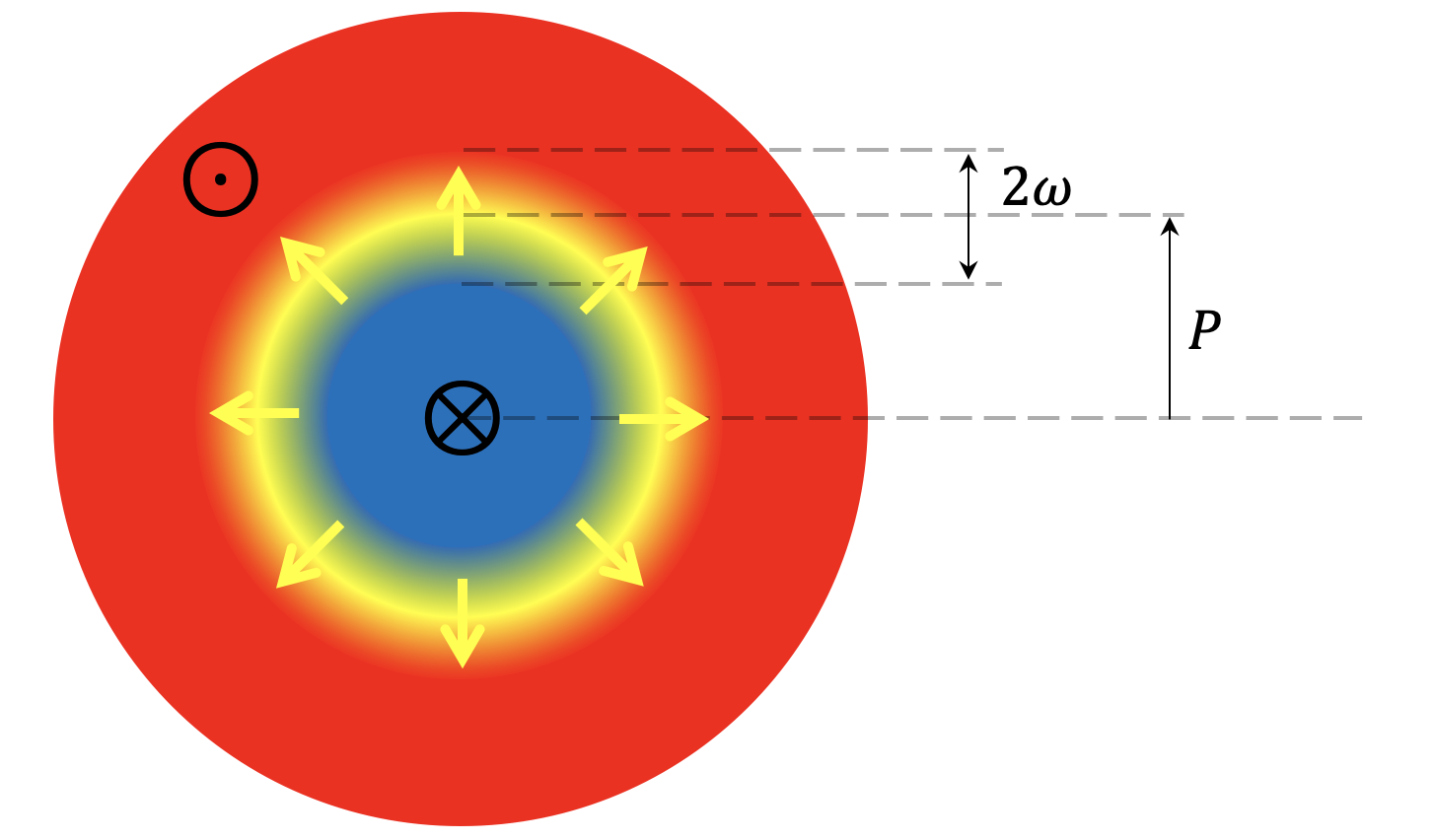
Figure 1: Skyrmion model with spin‐up (red) in the outer region, spin‐down (blue) in the inner region, and domain wall (yellow, located at $\rho=P$ with width $2\omega$) interpolating between them.

The continuous skyrmion model enables us to compute the Magnus and dissipative force tensors defined in (4). The former is $\mathcal{G}_{ij}=\epsilon_{ij}Q=\pm 4\pi\epsilon_{ij}$. For $\mathcal{D}_{ij}$, we first compute $\partial_{x}\vec{n}=(\partial_{x}\rho)\Theta^{\prime}(\rho)\big{(}\cos\Theta\hat{\rho}-\sin\Theta\hat{z}\big{)}-(\partial_{x}\phi)\sin\Theta\hat{\phi}$, where ^′ is $\rho$ derivative. Thus $(\partial_{x}\vec{n})^{2}=\cos^{2}\phi(\Theta^{\prime}(\rho))^{2}+(\sin^{2}\phi/\rho^{2})\sin^{2}\Theta$. These two terms only contribute for the DW region upon integration and depend on the ratio $\omega/P$. We omit the second term which is much smaller than the first, especially for the skyrmions with a skinny DW region, $\omega/P\ll 1$. Thus,

$$\begin{split}\mathcal{D}_{xx}&=-\int_{P-\omega}^{P+\omega}d\rho\rho\int_{0}^{2\pi}d\phi~{}\frac{\pi^{2}}{4\omega^{2}}\cos^{2}\phi=-\frac{\pi^{3}}{4}\frac{P}{\omega}\;.\end{split}$$ (18)

The diagonal components are the same $\mathcal{D}_{yy}=\mathcal{D}_{xx}\equiv D$ even with the omitted term. It is straightforward to check as $(\partial_{y}\vec{n})^{2}=\sin^{2}\phi(\Theta^{\prime}(\rho))^{2}+(\cos^{2}\phi/\rho^{2})\sin^{2}\Theta$, which gives the same result upon $\phi$ integral.

Now we check that the off diagonal components vanish, $\mathcal{D}_{xy}=\mathcal{D}_{yx}=0$. It is easy to see as $(\partial_{x}\vec{n})\cdot(\partial_{y}\vec{n})=((\Theta^{\prime}(\rho))^{2}-\sin^{2}\Theta/\rho^{2})\sin\phi\cos\phi$, which vanishes upon $\phi$ integral. Thus, we demonstrate the decomposition $\mathcal{D}_{ij}=D_{s}\delta_{ij}+D_{a}\epsilon_{ij}$ along with $D_{a}=0$.

$$\mathcal{D}_{ij}=D\,\delta_{ij}=-\frac{\pi^{3}}{4}\frac{P}{\omega}\;.$$ (19)

Note (15) gives $\tan\theta_{H}=Q/D$ for $R=0$ that reproduces the known fact that the positive- and negative-charge skyrmion Hall angles are the same with opposite signs.

One can also consider the Bloch-type skyrmions that has the parametrization $\Phi(\phi)=m\phi+\phi_{0}$, where $m$ is an integer representing the winding number and $\phi_{0}$ a constant phase. Similar computation, for example, gives $(\partial_{x}\vec{n})^{2}=\cos^{2}\phi(\Theta^{\prime}(\rho))^{2}+(m+1)^{2}(\sin^{2}\phi/\rho^{2})\sin^{2}\Theta$. Explicitly, it can be shown to $\mathcal{D}_{xx}=\mathcal{D}_{yy}=D$ and $\mathcal{D}_{xy}=\mathcal{D}_{yx}=0$. Thus, the dissipative tensor have the same results as in (19).

For the rest of the paper, we focus on investigating the consequences of the transverse velocity effect $R$ in the Hall angle (14).

$$\begin{split}&\tan\theta_{H}=\frac{Q+\alpha DR}{\alpha D-QR}\;.\end{split}$$ (20)

Before considering some physical systems, we note that $\tan\theta_{H}=R$ for $Q=0$. This tells that the positive- and negative-charge skyrmions have the same Hall angles (same transverse motion), for example, in anti-ferromagnetic materials.

First experimental data sets
There exist only a small number of systematic experimental data sets on Hall angles performed for both positive- and negative-charge skyrmions with the same environment Jiang2017 VanishingSkyrmionHall . First, we note that these available data sets consistently show significant, $6.5-12\%$, differences.

Let us start with VanishingSkyrmionHall as its data set is clearer to analyze for our purpose. The Hall angles were measured for Néel-type half skyrmions ($Q=\pm 2\pi$) in the ferrimagnetic GdFeCo/Pt films by utilizing the spin orbit torque (SOT) technique. The data set at temperature $T=343\,K$ is given as

$$\theta_{Q>0}=-35^{o}\;,\qquad\theta_{Q<0}=31^{o}\;,$$ (21)

with their $\%\,\text{difference}$ as

$$\%\,\text{difference}=12\%\;.$$ (22)

This is a strikingly large difference with naive expectation that the Hall angles between positive- and negative-charge skyrmions should be the same.

In Jiang2017 , the Hall angles for Néel-type positive- and negative-charge skyrmions were measured for Ta/CoFeB/TaO_x material, which shows strong pinning potential due to randomly distributed defects. When a ferromagnetic layer is placed on top of a heavy metal layer, polarized electric currents along the heavy metal layer can be used to pump spins into the ferromagnetic layer through the spin Hall effect. While the original data sets, figure $3\bf{c}$ in Jiang2017 , were collected for different magnetic fields $B$, careful interpolation was performed to obtain data at $B=\pm 5.0\,Oe$ that are presented in a table Kim:2020piv . The saturated Hall angles are $|\theta_{Q>0}|=31.6^{o}$ and $\theta_{Q<0}=29.3^{o}$ with their $\%\,\text{difference}=7.6\%$ for a pulse current. For the opposite current, $\%\,\text{difference}=5.5\%$. The combined, conservative, estimate for the difference between the positive- and negative-charge skyrmion Hall angles is $6.5\%$.

It is surprising to observe that there exist a large difference between the positive- and negative-charge skyrmion Hall angles (measured in the same environmental setup). Moreover, the former is consistently bigger than the latter. The original Hall angle formula (15) with $D_{a}=0$ is not suitable to describe these angles together. Here we would like to use (20) to estimate two parameters $\alpha D$ and $R$. These in turn can reveal the relative strength between the two transverse forces proportional to $Q$ and $\alpha DR$, which are two numerical terms in (20).

We start with $\theta_{Q>0}=-35^{o}$ for $Q=2\pi$ and $\theta_{Q<0}=31^{o}$ for $Q=-2\pi$ VanishingSkyrmionHall . By using (20) twice, we can estimate $\alpha D=-9.68$ and $R=-0.035$, where we use $\alpha D<0$. Thus the new contribution with $R$ is estimated to be

$$\frac{\alpha DR}{Q}=5.4\%\;.$$ (23)

Thus the transverse force due to the new transverse effect $R$ is about $5.4\%$ of the conventional skyrmion Hall effect, which is surprisingly large.

With the estimated values $\alpha D$ and $R$, we revisit the skyrmion Hall angle (20) to see the effects of the new terms introduced in (9). For a positive-charge skyrmion $Q>0$, the new term $\alpha DR>0$ enhances the transverse motion of the skyrmion, while the other new term $QR<0$ reduces its longitudinal motion. For a negative-charge skyrmion, the effect is opposite.

We turn to the data Jiang2017 , analyzed in detail Kim:2020piv , $\theta_{Q>0}=-31.6^{o}$ for $Q=4\pi$ and $\theta_{Q<0}=29.3^{o}$ for $Q=-4\pi$ for a current with $B=\pm 5\,Oe$. It is estimated to $\alpha D=-21.4$ and $R=-0.020$, which give $\alpha DR/Q=3.4\%$. Another data set, $\theta_{Q>0}=-32^{o}$ for $Q=4\pi$ and $\theta_{Q<0}=30.3^{o}$ for $Q=-4\pi$, for the opposite current gives $\alpha DR/Q=2.5\%$. The combined estimate is $\alpha DR/Q=2.9\%$.

Thus we conclude that, from two systematic experimental data sets, there exist an unexpected large difference: the positive-charge skyrmion Hall angle is $6.5-12\%$ larger than the negative-charge skyrmion Hall angle. The corresponding transverse force amounts to $2.9-5.4\%$ of the conventional Hall effect due to the skyrmion charge. These were analyzed before in Kim:2020piv .

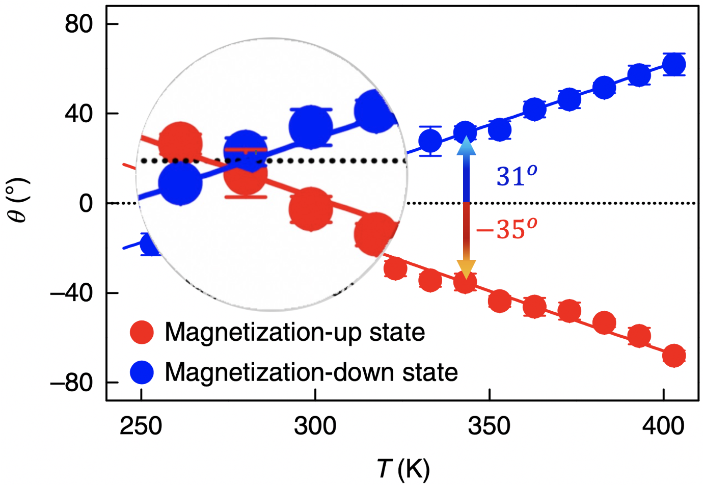
Figure 2: Systematic Hall angle data VanishingSkyrmionHall with enlargement around the angular momentum compensation temperature and the data set at $T=343\,K$. Magnetization-up state is identified as half skyrmion in VanishingSkyrmionHall and has $Q=-2\pi$ in our convention.

Second experimental data set
We return to VanishingSkyrmionHall as it has more interesting data, FIG. 2, for the positive- and negative-charge skyrmion Hall angles across the angular momentum compensation temperature $T_{A}\approx 283~{}K$ for a rare earth–3d-transition metal (ferrimagnetic) compound, GdFeCo/Pt film. The angular momentum compensation point is defined as the temperature when the spin densities of the two sub-compounds cancel each other as discussed below. For a clearer presentation, we also define another temperatures $\tilde{T}_{\pm}$, where the positive- and negative-charge skyrmion Hall angles vanish.

Before considering the Hall angle formula, we note interesting observations for FIG. 2,: (i) the positive-charge skyrmion Hall angles for $T>T_{A}$ are consistently larger than the negative-charge skyrmion angle as advertised above, (ii) the positive-charge skyrmion compensation temperature $(\tilde{T}_{+})$ is smaller than the negative-charge skyrmion one $(\tilde{T}_{-})$, and (iii) when the two Hall angles coincide, happening at $\tilde{T}_{0}$ ($\tilde{T}_{+}<\tilde{T}_{0}<\tilde{T}_{-}$), their values are negative, not vanishing. Thus, we can see that the Hall angle lines form a triangle with three vertices located at the three temperatures $\tilde{T}_{+},\tilde{T}_{0}$ and $\tilde{T}_{-}$. While the data are within the experimental uncertainties, the significant difference between the positive- and negative-charge skyrmion Hall angles deserves to investigate these observations further. More precision experiments will surely clarify these issues. The rest of the paper is devoted to look into them from a theoretical stand point.

Ferrimagnet compound is composed with two subnetworks of magnetization, $\vec{M}_{1}$ and $\vec{M}_{2}$, that are anti-ferromagnetically coupled through an effective local exchange field. While the gyromagnetic ratios $\gamma_{a}=M_{a}/s_{a}~{}(a=1,2)$ are constants as temperature changes, their magnet moments $\vec{M}_{a}$ and spin densities $\vec{s}_{a}$ of the two subnetworks change differently. There are two special temperatures, the magnetization compensation point where the net magnetization vanishes and the angular momentum compensation point ($T=T_{A}$), across which the net spin density $s_{n}(T_{A})=s_{1}(T_{A})-s_{2}(T_{A})=0$ changes its sign. Its general treatments using two independent magnetization vectors were developed in FerrimagnetFastMovongDomainWall FerrimagnetTheory1 . We note that the net spin density increases as temperature decreases.

When the exchange field is sufficiently large, the two magnetization vectors remain strongly coupled and anti-parallel to each other MMFerrimagnetBook . Thus, $\vec{\mu}=\vec{\mu}_{1}=-\vec{\mu}_{2}$ using the unit vectors $\mu_{a}$ as $\vec{M}_{a}=M_{a}\vec{\mu}_{a}$. We define the net magnetic moment $M_{n}=M_{1}-M_{2}$. The dynamics of $\vec{\mu}$ of the combined system can be described as

$$\begin{split}s_{n}\dot{\vec{\mu}}=-M_{n}\vec{\mu}\times\vec{H}_{\text{eff}}+s_{t}\alpha_{\text{eff}}\vec{\mu}\times\dot{\vec{\mu}}\;,\end{split}$$ (24)

where the net and total spin densities are $s_{n}=s_{1}-s_{2}$ and $s_{t}=s_{1}+s_{2}$, respectively. $\alpha_{\text{eff}}=(\alpha_{1}s_{1}+\alpha_{2}s_{2})/(s_{1}+s_{2})$ is the effective damping parameter.

We are ready to apply our generalized Hall angle (20) for the experimental data in FIG. 2. (24) is simpler, yet consistent with the model adapted in VanishingSkyrmionHall , which used the Magnus force as $\vec{F}_{g}=s_{n}Q(\hat{z}\times\vec{v})$ and the viscose force as $\vec{F}_{d}=s_{t}\alpha D\vec{v}$. Thus, the spin (and temperature) dependence can be incorporated by $Q\to s_{n}Q$ and $\alpha D\to s_{t}\alpha D$. Thus,

$$\tan\theta_{H}=\frac{s_{n}Q+s_{t}\alpha DR}{s_{t}\alpha D-s_{n}QR}\;.$$ (25)

When $R=0$, $\tan\theta_{H}=s_{n}Q/s_{t}\alpha D$, which vanishes at the compensation temperature as $s_{n}(T_{A})=0$. The positive- and negative-charge skyrmion Hall angles are the same (with opposite signs).

We highlight the Hall angle (25), among its interesting details, with its dependence on the spin densities. It only depends on the combination $s_{n}/s_{t}$, which turns out to be a monotonically decreasing function of temperature $T$. By analyzing the data (21) at $T=343\,K$, we arrive the same estimates $(s_{t}/s_{n})(\alpha DR/Q)=5.4\%$ in (23), along with $R=-0.035$ and $(s_{t}/s_{n})(\alpha D)=-9.68$ footnote .

Let us look at the Hall angle (25) more carefully near the compensation point as a function of $s_{n}/s_{t}$.

• When $s_{n}=0$, that happens $T=T_{A}$,

  $$\tan\theta_{H}=R\;.$$ (26)

  The two Hall angles are the same at $T=\tilde{T}_{0}$ and negative as $R<0$. Thus $\tilde{T}_{0}$ coincide with the compensation temperature $T_{A}$.

• The positive- and negative-charge skyrmion Hall angles vanish at different temperatures as they happen when $s_{n}Q+s_{t}\alpha DR=0$. In terms of spin densities,

  $$\frac{s_{n}}{s_{t}}\Big{|}_{T=\tilde{T}_{\pm}}=-\frac{\alpha DR}{Q}\;.$$ (27)

  Note also vanishing Hall angle temperatures $\tilde{T}_{\pm}$ do not coincide with the compensation temperature $T_{A}$. The positive-charge skyrmion Hall angle vanishes when $s_{n}/s_{t}>0$ (thus $\tilde{T}_{+}<T_{A}$), while the negative-charge skyrmion one vanishes when $s_{n}/s_{t}<0$ (thus $\tilde{T}_{-}>T_{A}$), where we use $\alpha D>0$ and $R<0$ footnote .

From a) and b), we confirm that these three different temperatures ($\tilde{T}_{A+}<\tilde{T}_{0}<\tilde{T}_{A-}$) serve as vertices of the triangle mentioned above for FIG. 2.

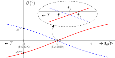
Figure 3: Plot generated for $\theta_{H}$ given in (25) as a function of $s_{n}/s_{t}$, which is a decreasing function of $T$. Solid red line is for skyrmion, while dashed blue for antiskyrmion. This plot captures the essential features of the experimental data presented in figure 4 in VanishingSkyrmionHall .

Finally, we plot the positive-charge (red) and negative-charge (blue) skyrmion Hall angles in FIG. 3 as a function of $s_{n}/s_{t}$ for the range $-1.5\leq s_{n}/s_{t}\leq 1.5$. Here we use constant values for $R$ and $\alpha D$ obtained at the reference point $s_{n}/s_{t}=-1$ at $T=343\,K$. We note that this plot captures essential features of the experimental Hall angle data as a function of spin density that is presented in figure 4 of VanishingSkyrmionHall . In addition, the inset of FIG. 3, that manifests the triangle near the compensation point, is consistent with FIG. 2.

What accounts for the transverse velocity?
In this paper we have generalized the Thiele equation with the transverse velocity effect introduced in (5) and demonstrated its usefulness for describing the surprising mismatches ($6.5-12\%$) between the positive- and negative-charge skyrmion Hall angles. In particular, this new transverse force accounts for $2.9-5.4\%$ of the conventional skyrmion Hall effect. Moreover, our generalized Hall angle formula (25) (also (20)) reproduces a non-trivial experimental Hall angle data in the context of the ferrimagnetic compound near the compensation point. See FIG. 3.

One can ask whether there is a physical motivation for introducing the transverse velocity component $R$ to the Thiele equation. The answer is affirmative.

Recent study of Hydrodynamics revealed that there exists a universal transport coefficient, Hall viscosity Avron:1995 , in the absence of mirror (parity) symmetry Jensen:2011xb Bhattacharya:2011tra . It has been extensively studied theoretically in quantum Hall systems and linked to a half of the system’s angular momentum density Read:2008rn or Hall conductivity Hoyos:2011ez . More systematic relations were studied in Bradlyn:2012ea Hoyos:2014lla .

This Hall viscosity was introduced to skyrmion motion, whose systems also have broken parity, by utilizing the topological Ward identity Kim:2015qsa Kim:2019vxt KimBook . It is transverse to the skyrmion’s motion and dissipationless. Moreover, the analysis of Kubo formula tells that Hall viscosity does not depend on skyrmioin charges and thus pushes the positive- and negative-charge skyrmions toward the same transverse direction Kim:2020piv . Once added to the skyrmion Hall effect, the positive-charge skyrmion Hall angle is bigger than that of the negative-charge skyrmion.Thus, we can conclude the effect of Hall viscosity is estimated to be $2.9-5.4\%$ of the conventional skyrmion Hall effect according to our analysis. Precision skyrmion experiments focused on the positive- and negative-charge skyrmion Hall angles are an ideal ground for reliably confirming the existence of Hall viscosity!

Acknowledgments: This work has been partially supported by Wisys Spark grant and UW-Parkside summer research funds. We thank to the anonymous referees’ comments, which improve the paper’s clarity.

References

- (1) A. A. Thiele, Steady-State Motion of Magnetic Domains. Phys. Rev. Lett. 30, 230 (1973).
- (2) B. S. Kim, Modeling Hall viscosity in magnetic-skyrmion systems. Phys. Rev. Res. 2, 013268 (2020)
- (3) L. D. Landau and E. M. Lifshitz, Fluid Mechanics, Third Impression. Pergamon Press Ltd. (1966).
- (4) T. L. Gilbert, A phenomenological theory of damping in ferromagnetic materials. IEEE Trans. Magn. 40, 3443 (2004).
- (5) Y. Shu et. al., Realization of the skyrmionic logic gates and diodes in the same racetrack with enhanced and modified edges. Appl. Phys. Lett., 121, 042402 (2022) and references therein.
- (6) L. Shen et. al., Spin torque nano-oscillators based on antiferromagnetic skyrmions. Appl. Phys. Lett. 114, 042402 (2019).
- (7) L. Shen et. al., Current-Induced Dynamics and Chaos of Antiferromagnetic Bimerons. Phys. Rev. Lett. 124, 037202 (2020).
- (8) B. S. Kim, Skyrmions and Hall Transport. (394 pages) Jenny Stanford Publishing (2023).
- (9) W. Jiang et. al., Direct Observation of the Skyrmion Hall effect. Nature Physics 13, 162 (2017).
- (10) Here we use a slightly different definition for skyrmion charge with an extra compared to SKCharge . Moreover, we point out that there are different conventions for defining skyrmion and antiskyrmion as illustrated in Fig. 2.4 of Han and explained there. To remove further confusions, we use the term positive- and negative-charge skyrmions when it is necessary to distinguish them. For comparison below, we also mention that the Magnetization-up state defined in Fig 3 and Fig.4 of VanishingSkyrmionHall has .
- (11) X. Zhang et. al., Skyrmion-electronics: writing, deleting, reading and processing magnetic skyrmions toward spintronic applications. J. Phys.: Condens. Matter 32 143001 (2020).
- (12) J. H. Han, Skyrmions in Condensed Matter. Springer (2017).
- (13) Y. Hirata et. al, Vanishing skyrmion Hall effect at the angular momentum compensation temperature of a ferrimagnet. Nature Nanotechnology 14, 232 (2019)
- (14) K.-J Kim, et al., Fast domain wall motion in the vicinity of the angular momentum compensation temperature of ferrimagnets. Nature Mater 16 (2017) 1187.
- (15) S. K. Kim, K.-J. Lee, and Y. Tserkovnyak, Self-focusing skyrmion racetracks in ferrimagnets. Phys. Rev. B 95, (2017) 140404(R)
- (16) M. Mansuripur, The Physical Principles of Magneto-optical Recording. Cambridge University Press, 1998.
- (17) J. E. Avron, R. Seiler and P. G. Zograf, Viscosity of Quantum Hall Fluids. Phys. Rev. Lett. 75, 697 (1995).
- (18) K. Jensen et al., Parity-Violating Hydrodynamics in 2+1 Dimensions. JHEP 1205, 102 (2012).
- (19) J. Bhattacharya, S. Bhattacharyya, S. Minwalla and A. Yarom, A Theory of first order dissipative superfluid dynamics. JHEP 1405, 147 (2014).
- (20) N. Read, Non-Abelian adiabatic statistics and Hall viscosity in quantum Hall states and paired superfluids. Phys. Rev. B 79, 045308 (2009).
- (21) C. Hoyos and D. T. Son, Hall Viscosity and Electromagnetic Response. Phys. Rev. Lett. 108, 066805 (2012).
- (22) B. Bradlyn, M. Goldstein and N. Read, Kubo formulas for viscosity: Hall viscosity, Ward identities, and the relation with conductivity. Phys. Rev. B 86, 245309 (2012)
- (23) C. Hoyos, B. S. Kim and Y. Oz, Ward Identities for Hall Transport. JHEP 1410, 054 (2014)
- (24) B. S. Kim and A. D. Shapere, Skyrmions and Hall Transport. Phys. Rev. Lett. 117, 116805 (2016).
- (25) B. S. Kim, Topical Review on Skyrmions and Hall Transport. J. Phys.: Condens. Matter 31, 383001 (2019)
- (26) We note at in our convention. To analyze Hall angles and other quantities as a function of , we need to set and . This is consistent with the estimates near (23).