Strong-field scattering of two spinning black holes: Numerical Relativity versus post-Minkowskian gravity

Abstract

Highly accurate models of the gravitational-wave signal from coalescing compact binaries are built by completing analytical computations of the binary dynamics with non-perturbative information from numerical relativity (NR) simulations. In this paper we present four sets of NR simulations of equal-mass black hole binaries that undergo strong-field scattering: (i) we reproduce and extend the nonspinning simulations first presented in [Damour et al., Phys.Rev.D 89 (2014) 8, 081503], (ii) we compute two suites of nonspinning simulations at higher energies, probing stronger field interactions, (iii) we present a series of spinning simulations including, for the first time, unequal-spin configurations. When comparing the NR scattering angles to analytical predictions based on state-of-the-art post-Minkowskian (PM) calculations, we find that PM-expanded scattering angles show poor convergence towards NR data. By contrast, a resummed computation of scattering angles via a spin-dependent, radiation-reacted, effective-one-body potential shows excellent agreement for both nonspinning and spinning configurations.

I Introduction

The detection and characterisation of gravitational-wave (GW) observations Abbott et al. (2019, 2021a, 2021b); Nitz et al. (2023); Olsen et al. (2022) from compact binary coalescences relies on theoretical predictions of the emitted signal. Highly accurate models of coalescing compact binaries are a crucial requirement to perform precise measurements of the properties of black holes (BHs) and neutron stars, to determine their underlying astrophysical distributions and to perform tests of General Relativity in the strong-field regime. Such waveform models are generally built using both analytical and numerical approximations to Einstein’s equations for a binary system in quasi-circular orbits.

Numerical Relativity (NR) simulations of quasi-circular binaries Pretorius (2005); Campanelli et al. (2006a); Mroue et al. (2013); Husa et al. (2016); Jani et al. (2016); Boyle et al. (2019); Healy et al. (2019); Hamilton et al. (2023) provide the most accurate representation of the emitted waveform, especially during the plunge, merger and ringdown phases. Such simulations can be used to build NR surrogates Field et al. (2014); Blackman et al. (2017); Varma et al. (2019), whose main limitation is their restricted parameter space coverage.

Semi-analytical GW approximants, such as effective-one-body (EOB) Buonanno and Damour (1999, 2000); Gamba et al. (2022a); Ossokine et al. (2020); Ramos-Buades et al. (2023) and phenomenological models Hannam et al. (2014); Pratten et al. (2020); García-Quirós et al. (2020); Pratten et al. (2021); Hamilton et al. (2021), use a combination of numerical and analytical information. These approximants generally make use of the post-Newtonian (PN) expansion Blanchet and Damour (1989); Blanchet (2014); Damour et al. (2014a); Levi and Steinhoff (2016); Bini and Damour (2017a); Schaefer and Jaranowski (2018); Bini et al. (2019, 2020a, 2020b, 2020c); Antonelli et al. (2020); Blümlein et al. (2021, 2022); Mandal et al. (2023a, b), which assumes small velocities ($v/c\ll 1$) together with weak fields [$GM/(rc^{2})\ll 1$], making it apt to describe quasi-circular inspirals. However, with the improving sensitivity of current detectors and ongoing development of a third generation of GW detectors Reitze et al. (2019); Punturo et al. (2010); Amaro-Seoane et al. (2017), the possibility of detecting eccentric binaries and hyperbolic encounters has risen in prominence Romero-Shaw et al. (2020); Bustillo et al. (2021); Gayathri et al. (2022); Gamba et al. (2022b). The detection and characterization of binaries on non-circular orbits is thought to be a powerful tracer for constraining the formation and evolution channels of astrophysical BHs O’Leary et al. (2006, 2009); Samsing et al. (2014); Rodriguez et al. (2016); Belczynski et al. (2016); Samsing (2018); Romero-Shaw et al. (2019); Zevin et al. (2021).

Analytical models of non-circular binaries cannot solely rely on the PN approximation, as the two bodies could already possess high velocities at large separations. In these situations, the post-Minkowskian (PM) approximation Damour (2016, 2018), which only assumes weak fields [$GM/(rc^{2})\ll 1$] while allowing for large velocities, is more appropriate. PM contributions have been computed using various approaches to gravitational scattering, such as: scattering amplitudes (see, e.g., Cheung et al. (2018); Guevara et al. (2019a); Kosower et al. (2019); Bern et al. (2019a, b, a); Bjerrum-Bohr et al. (2020); Herrmann et al. (2021); Bern et al. (2021a, 2022); Bjerrum-Bohr et al. (2021); Manohar et al. (2022); Saketh et al. (2022)); eikonalization (e.g., Koemans Collado et al. (2019); Di Vecchia et al. (2020, 2021, 2022)); effective field theory (e.g., Kälin and Porto (2020a); Kälin et al. (2020); Mougiakakos et al. (2021); Dlapa et al. (2022a, b); Kälin et al. (2023); Dlapa et al. (2023)); and worldline (classical or quantum) field theory (e.g., Mogull et al. (2021); Riva and Vernizzi (2021); Jakobsen et al. (2021, 2022); Bini et al. (2021); Bini and Damour (2022); Bini et al. (2023)). The resulting terms can be incorporated into semi-analytic models to improve their accuracy for binaries on eccentric and hyperbolic orbits Chiaramello and Nagar (2020); Nagar et al. (2021); Placidi et al. (2022); Khalil et al. (2021); Ramos-Buades et al. (2022a); Nagar and Rettegno (2021); Khalil et al. (2022). At the same time, numerical results are necessary to determine the accuracy and validity of these approximations. Whilst a large suite of numerical simulations of binary black holes (BBHs) on eccentric orbits have been performed Hinder et al. (2010); Gold et al. (2012); Lewis et al. (2017); Ramos-Buades et al. (2020); Huerta et al. (2019); Habib and Huerta (2019); Gayathri et al. (2022); Islam et al. (2021); Ramos-Buades et al. (2022b), there are comparatively few simulations regarding BBH scattering  Shibata et al. (2008); Sperhake et al. (2009); Damour et al. (2014b); Hopper et al. (2023); Healy and Lousto (2023).

The aims of this paper are: (i) to extend the results of Ref. Damour et al. (2014b) by performing higher-initial-energy NR simulations of equal-mass nonspinning BBH scattering; (ii) to perform NR simulations of the scattering of equal-mass spinning BBHs, both for equal and unequal spins, aligned with the angular momentum; and (iii) to compare the so-obtained strong-field numerical scattering angles to analytical predictions based on state-of-the-art PM results.

We denote the masses of the two objects as $m_{1}$ and $m_{2}$, and the individual dimensionless spins as $\chi_{i}=S_{i}/(Gm_{i}^{2})=a_{i}/(Gm_{i})$, $i=1,2$. In addition, we denote $M=m_{1}+m_{2}$, $\mu={m_{1}m_{2}}/{(m_{1}+m_{2})}$, $\nu={\mu}/{M}={m_{1}m_{2}}/{(m_{1}+m_{2})^{2}}$. All our simulations will have $m_{1}=m_{2}$, so that $\nu=1/4$. Throughout this paper, we denote the canonical orbital angular momentum simply as $L$. It is related to the total Arnowitt-Deser-Misner (ADM) angular momentum of the system, $J$, by

$$J=L+S_{1}+S_{2}\,.$$ (1)

Unless otherwise stated, we take $G=c=1$ and generally work with dimensionless quantities.

II Numerical Relativity (NR) Simulations

We performed several sequences of nonspinning and spin-aligned NR simulations modelling the scattering of two equal mass BHs. The numerical simulations were performed using the Einstein Toolkit (ETK) et al. (2022), an open source numerical relativity code built on the Cactus framework. The numerical setup of our simulations is broadly similar to that used in Damour et al. (2014b), though we present the details here for completeness.

We use Bowen-York initial data Bowen and York (1980); Brandt and Brügmann (1997) computed using the TwoPunctures thorn Ansorg et al. (2004). As in Damour et al. (2014b), the BHs are initially placed on the $x$-axis at a separation of $\pm X$ and with initial ADM linear momenta

$$\vec{P}=(P_{x},P_{y},P_{z})=\pm\,P_{\rm ADM}\left(-\sqrt{1-\left(\frac{b_{\rm NR}}{2X}\right)^{2}},\frac{{b}_{\rm NR}}{2X},0\right).$$ (2)

where $P_{\rm ADM}=|\vec{P}|$ and $b_{\rm NR}$ denotes an impact parameter. As in Damour et al. (2014b), we use $X=50M$. The Bowen-York initial data determine both the initial total ADM energy $E^{\rm ADM}_{\rm in}$ of the system, and the total initial ADM angular momentum of the system. The latter is given by the simple formula

$$J^{\rm ADM}_{\rm in}=L_{\rm in}+S_{1}+S_{2}\,,$$ (3)

where the initial canonical orbital angular momentum $L_{\rm in}$ is related to $b_{\rm NR}$ and $P_{\rm ADM}$ by Damour et al. (2014b)

$$L_{\rm in}=2X|P_{y}|=\,P_{\rm ADM}\,b_{\rm NR}\,.$$ (4)

We adopt as initial lapse profile $\alpha=\psi^{-2}_{\rm BL}$, where $\psi_{\rm BL}$ denotes the Brill-Lindquist conformal factor Brandt and Brügmann (1997); Alcubierre et al. (2003); Campanelli et al. (2006a). In Appendix A, we present a check that the uncertainty linked to the choice of initial lapse profile has a subdominant effect on the inferred scattering angle $\theta_{\rm NR}$ compared to the errors in the polynomial fits used to measure the scattering angle.

Time evolution is performed using the $W$-variant Marronetti et al. (2008) of the BSSNOK formulation (Shibata and Nakamura, 1995; Baumgarte and Shapiro, 1999; Nakamura et al., 1987) of the Einstein field equations as implemented by the McLachlan Brown et al. (2009) thorn. We evolve the BHs using moving punctures gauge conditions Baker et al. (2006); Campanelli et al. (2006a), the lapse is evolved using the $1+\log$ condition Bona et al. (1995), and the shift is evolved using the hyperbolic $\tilde{\Gamma}$-driver equation Alcubierre et al. (2003). We use eight-order accurate finite differencing stencils with Kreiss-Oliger dissipation Kreiss and Oliger (1973). Adaptive mesh refinement is provided by Carpet, with the near zone being computed with high-resolution Cartesian grids that track the motion of the BHs and the wave extraction zone being computed on spherical grids using the Llama multipatch infrastructure Pollney et al. (2011). The apparent horizons are computed using AHFinderDirect Thornburg (2004) and the spin angular momenta are calculated using the dynamical horizon formalism provided by the QuasiLocalMeasures thorn Dreyer et al. (2003).

Similarly to Damour et al. (2014b), we found that the total energy and angular momentum of the system left after the release of the burst of spurious radiation present in the initial data differ from the corresponding ADM quantities computed from the initial data only by negligible fractions of order $10^{-5}$.

All ETK simulations were managed using Simulation Factory Allen et al. and post-processing of NR data has made used of the open source Mathematica package Simulation Tools Hinder and Wardell .

II.1 Extracting the Scattering Angle

In order to calculate the scattering angle, we follow the prescription detailed in Damour et al. (2014b). The motion of the BHs is tracked by the Cartesian coordinates of the punctures in the center-of-mass frame. We convert the tracks to polar coordinates $(r,\varphi)$ (in the $x-y$ plane of motion) for each BH and treat the incoming $\varphi_{{\rm in},i}(r)$ and outgoing $\varphi_{{\rm out},i}(r)$ paths for the $i$-th BH separately. We fit each of the paths to a polynomial of order $n$ in terms of $u=1/r$ and extrapolate to find the asymptotic angle $\varphi^{\infty}_{{\rm in/out},i}$. The resulting scattering angle for the $i$-th particle is given by

$$\theta_{i}=\varphi^{\infty}_{{\rm out},i}-\varphi^{\infty}_{{\rm in},i}-\pi\,.$$ (5)

Our choice of fitting window for $(u,\varphi)$ follows Damour et al. (2014b), and we assume $r\in[14,80]M$ and $r\in[20,100]M$ for the incoming and outgoing trajectories respectively. We implement a least-squares fitting method that uses a singular value decomposition (SVD) to drop singular values smaller than $10^{-13}$ times the maximum singular value, as was used in Damour et al. (2014b). In order to gauge the errors on the scattering angle, we perform a number of sanity checks. The first check is to gauge the impact of the polynomial order $n$ on the resulting scattering angle. As in Damour et al. (2014b), the preferred polynomial order is taken to be the lowest order for which the SVD method allows for variation in the constant term. The extrapolation error is then estimated by finding the maximum and minimum scattering angle inferred over all polynomial orders between $2$ and $n-1$. This generally leads to dissymmetric error bounds on the scattering angle: $\theta^{+\delta_{+}}_{-\delta_{-}}$. A value of $0$ in $\delta_{+}$ or $\delta_{-}$ occurs when the preferred polynomial is setting the bound. More precisely, $\delta_{-}=0$ (respectively $\delta_{+}=0$) occurs when the lower order polynomial fits over-estimate (respectively, under-estimate) the scattering angle relative to the preferred order. When least-square fitting our numerical results to analytical templates, we shall use a symmetrized version of the error bounds, namely $\pm\frac{1}{2}(\delta_{+}+\delta_{-})$.

Other sanity checks on the robustness of the derived scattering angle include testing the impact of the fitting window, testing the resolution of our numerical simulations, and varying gauge choices in the numerical evolution. We find that the inferred errors on the scattering angle remain subdominant to the choice of polynomial order, in agreement with the conclusions in Damour et al. (2014b). See Appendix A for further details.

II.2 Nonspinning Scattering Simulations

Though the main aim of the present work is to simulate the scattering of spinning BBHs, we also performed systematic sequences of nonspinning simulations of BBHs with fixed initial energy and varying initial angular momenta in order to be able to extract direct numerical estimates of the EOB interaction potential (see Sec. V below). For the first sequence, we reproduced and extended the results of Ref. Damour et al. (2014b), with an initial (adimensionalized) ADM energy $\hat{E}^{\rm ADM}_{\rm in}\equiv E_{\rm in}^{\rm ADM}/M$ equal to $\hat{E}^{\rm ADM}_{\rm in,1}\simeq 1.02264$ and varying initial (rescaled) orbital angular momentum $\hat{L}_{\rm in}\equiv L_{\rm in}/M^{2}$. This allowed us both to cross-check the accuracy of our computations and to probe more precisely the boundary between scattering and plunge. We also performed two more sequences at the higher incoming energies, $\hat{E}_{\rm in,2}^{\rm ADM}\simeq 1.04033$ and $\hat{E}_{\rm in,3}^{\rm ADM}\simeq 1.05548$. These explore a stronger-field region of the parameter space, with NR impact parameters going down to $\hat{b}_{\rm NR}\equiv b_{\rm NR}/M\simeq 6$ (with corresponding minimum isotropic EOB radial coordinate $\bar{r}^{\rm min}\simeq 2$, see below).

We report the results of all our nonspinning simulations in Table 1. In Fig. 1 we show the scattering angles versus the impact parameter $\hat{b}_{\rm NR}$ for all three series of nonspinning systems. For the nonspinning simulations, we have that $\theta_{\rm NR}=\theta_{1}=\theta_{2}$.

Table 1: Equal-mass, nonspinning NR simulations. The scattering angles have been replaced by dots where the BHs have plunged. An asterisk denotes simulations where there is uncertainty on an eventual plunge. Longer simulations are required to determine whether the system becomes bound after the first encounter.

$\hat{b}_{\rm NR}$	$\hat{E}_{\rm in}^{\rm{ADM}}$	$\hat{L}_{\rm in}^{\rm{ADM}}$	$\theta_{\rm{NR}}\left[\rm deg\right]$
9.40	1.02264	1.07690	$\cdots$
9.50	1.02264	1.08840	$\phantom{\ast}376.275^{+0.026}_{-14.69}\ast$
9.55	1.02264	1.09410	$329.057^{+0.003}_{-1.534}$
9.56	1.02264	1.09520	$323.422^{+0.000}_{-1.914}$
9.57	1.02264	1.09640	$318.394^{+0.000}_{-1.575}$
9.58	1.02264	1.09750	$313.764^{+0.000}_{-1.331}$
9.60	1.02264	1.09980	$305.734^{+0.056}_{-0.694}$
9.70	1.02264	1.11130	$274.368^{+0.074}_{-0.016}$
9.90	1.02264	1.13420	$235.447^{+0.912}_{-0.003}$
10.00	1.02264	1.14560	$221.823^{+0.762}_{-0.002}$
10.20	1.02264	1.16860	$200.810^{+0.620}_{-0.004}$
10.40	1.02264	1.19150	$184.684^{+0.221}_{-0.002}$
11.00	1.02264	1.26020	$152.106^{+0.055}_{-0.446}$
12.00	1.02264	1.37480	$120.804^{+0.013}_{-0.307}$
13.00	1.02264	1.48930	$101.616^{+0.059}_{-0.002}$
14.00	1.02264	1.60390	$88.260^{+0.337}_{-0.002}$
15.00	1.02264	1.71850	$78.296^{+0.520}_{-0.002}$
16.00	1.02264	1.83300	$70.404^{+0.927}_{-0.003}$
7.67	1.04032	1.15050	$\cdots$
7.73	1.04032	1.15950	$\phantom{\ast}392.815^{+0.006}_{-7.477}\ast$
7.77	1.04032	1.16550	$338.973^{+0.156}_{-0.756}$
7.80	1.04032	1.17000	$317.637^{+0.142}_{-0.444}$
7.87	1.04032	1.18050	$283.359^{+0.343}_{-0.007}$
7.93	1.04032	1.18950	$262.825^{+0.749}_{-0.008}$
8.00	1.04032	1.20000	$244.210^{+1.220}_{-0.005}$
8.40	1.04033	1.26000	$184.138^{+0.439}_{-0.004}$
8.80	1.04033	1.32000	$153.119^{+0.226}_{-0.227}$
9.00	1.04033	1.35000	$141.986^{+0.244}_{-0.213}$
9.40	1.04033	1.41000	$124.805^{+0.154}_{-0.238}$
9.50	1.04033	1.42500	$121.233^{+0.180}_{-0.153}$
9.60	1.04033	1.44000	$117.897^{+0.157}_{-0.091}$
10.00	1.04033	1.50000	$106.459^{+0.207}_{-0.004}$
12.00	1.04033	1.80000	$73.095^{+1.358}_{-0.006}$
14.00	1.04033	2.10000	$56.489^{+1.242}_{-0.006}$
16.00	1.04033	2.40000	$45.982^{+1.530}_{-0.008}$
6.00	1.05548	1.05000	$\cdots$
7.00	1.05548	1.22500	$354.118^{+0.307}_{-0.633}$
7.20	1.05548	1.26000	$248.950^{+1.203}_{-0.005}$
7.40	1.05548	1.29500	$206.064^{+1.479}_{-0.006}$
7.60	1.05548	1.33000	$179.815^{+0.484}_{-0.006}$
8.00	1.05548	1.40000	$146.516^{+0.354}_{-0.096}$
9.00	1.05548	1.57500	$104.166^{+0.361}_{-0.006}$
10.00	1.05548	1.75000	$82.275^{+0.924}_{-0.007}$
11.00	1.05548	1.92500	$68.351^{+1.485}_{-0.007}$

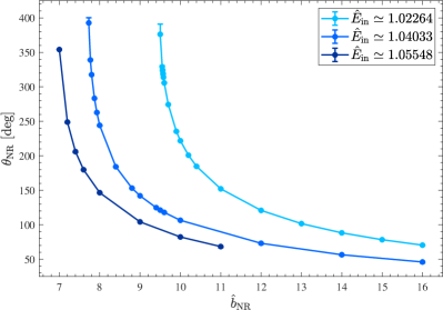
Figure 1: NR scattering angles against impact parameter for the (equal-mass) nonspinning simulations. Higher-energy systems are able to probe stronger fields (smaller separations) without plunging.

II.3 Spinning Scattering Simulations

We present here the results of 35 NR simulations of hyperbolic encounters of (equal-mass) spinning BBHs. As far as we know, it is the first time unequal-spin simulations have been published. In particular, we compute a suite of simulations at fixed energy and (canonical) orbital angular momentum and various spin magnitudes. The main parameters of these simulations are reported in Table 2, while the scattering angles, as a function of the rescaled spin variables $\chi_{i}$ are shown in Fig. 2.

When unequal spins are considered, the system ceases to be symmetric, inducing a non-zero recoil on the system center-of-mass. The effect of recoil on the scattering has been investigated in Ref. Bini et al. (2021). As a consequence of Eq. (3.33) there, the scattering angles measured using the individual trajectories of the two bodies will be different. In the following, we will denote by $\theta_{\rm NR}$ the relative scattering angle, which, for equal-mass binaries, is simply given (to linear order in the recoil) by

$$\theta_{\rm NR}=\frac{\theta_{1}+\theta_{2}}{2}\,.$$ (6)

Table 2: NR equal-mass, spinning simulations with (approximately) fixed incoming energy $\hat{E}_{\rm in}^{\rm{ADM}}\simeq 1.02264$ and fixed orbital angular momentum $\hat{L}_{\rm in}^{\rm{ADM}}=1.14560$. The columns, from left to right, represent: the individual spins; the incoming (rescaled) ADM energy; the incoming (rescaled) orbital ADM angular momentum; the scattering angle of the two individual objects (replaced by dots when the objects plunge); and the average scattering angle $\theta_{\rm{NR}}$ with its two-sided uncertainty.

$\chi_{1}$	$\chi_{2}$	$\hat{E}_{\rm in}^{\rm{ADM}}$	$\theta_{1}\left[\rm deg\right]$	$\theta_{2}\left[\rm deg\right]$	$\theta_{\rm{NR}}\left[\rm deg\right]$
-0.30	-0.30	1.02269	$\cdots$	$\cdots$	$\cdots$
-0.25	-0.25	1.02268	367.529	367.562	$\phantom{\ast}367.545^{+0.000}_{-4.840}\ast$
-0.23	-0.23	1.02267	334.344	334.346	$334.345^{+0.084}_{-1.573}$
-0.22	-0.22	1.02267	322.693	322.693	$322.693^{+0.099}_{-1.004}$
-0.21	-0.21	1.02267	312.795	312.795	$312.795^{+0.187}_{-0.364}$
-0.20	-0.20	1.02266	303.910	303.858	$303.884^{+0.222}_{-0.466}$
-0.17	-0.17	1.02266	286.603	286.604	$286.603^{+0.154}_{-0.010}$
-0.16	-0.16	1.02266	277.848	277.850	$277.849^{+0.230}_{-0.003}$
-0.15	-0.15	1.02265	272.602	272.603	$272.603^{+0.260}_{-0.003}$
-0.10	-0.10	1.02265	251.027	251.029	$251.028^{+0.559}_{-0.003}$
-0.05	-0.05	1.02264	234.747	234.389	$234.568^{+0.845}_{-0.003}$
-0.00	-0.00	1.02264	221.822	221.823	$221.823^{+0.762}_{-0.002}$
-0.05	-0.05	1.02264	211.195	211.195	$211.195^{+0.610}_{-0.002}$
-0.05	-0.05	1.02264	221.950	221.782	$221.866^{+0.643}_{-0.002}$
-0.10	-0.10	1.02265	202.763	202.453	$202.608^{+0.388}_{-0.002}$
-0.15	-0.15	1.02265	194.542	194.542	$194.542^{+0.183}_{-0.001}$
-0.15	-0.15	1.02265	222.141	221.632	$221.887^{+0.637}_{-0.002}$
-0.20	-0.20	1.02266	222.148	221.490	$221.819^{+0.863}_{-0.003}$
-0.20	-0.20	1.02266	187.839	187.838	$187.838^{+0.020}_{-0.141}$
-0.30	-0.30	1.02269	176.588	176.585	$176.586^{+0.001}_{-0.653}$
-0.40	-0.40	1.02274	222.488	221.206	$221.847^{+0.849}_{-0.003}$
-0.40	-0.00	1.02269	188.456	187.819	$188.138^{+0.008}_{-0.132}$
-0.40	-0.40	1.02274	167.545	167.544	$167.545^{+0.002}_{-0.947}$
-0.50	-0.30	1.02275	203.759	202.484	$203.121^{+0.477}_{-0.002}$
-0.60	-0.60	1.02288	223.008	221.153	$222.080^{+0.808}_{-0.003}$
-0.60	-0.00	1.02276	178.087	177.170	$177.629^{+0.001}_{-0.645}$
-0.60	-0.60	1.02288	154.139	154.139	$154.139^{+0.005}_{-1.443}$
-0.70	-0.30	1.02284	191.175	189.640	$190.407^{+0.013}_{-0.164}$
-0.70	-0.30	1.02284	161.186	160.685	$160.935^{+0.004}_{-1.274}$
-0.80	-0.80	1.02309	222.855	220.504	$221.679^{+0.489}_{-0.002}$
-0.80	-0.50	1.02294	199.960	198.026	$198.993^{+0.237}_{-0.001}$
-0.80	-0.00	1.02287	170.873	169.914	$170.394^{+0.003}_{-1.026}$
-0.80	-0.20	1.02288	162.421	161.716	$162.069^{+0.005}_{-1.308}$
-0.80	-0.50	1.02295	152.464	152.143	$152.303^{+0.006}_{-1.640}$
-0.80	-0.80	1.02309	145.467	145.248	$145.357^{+0.006}_{-1.528}$

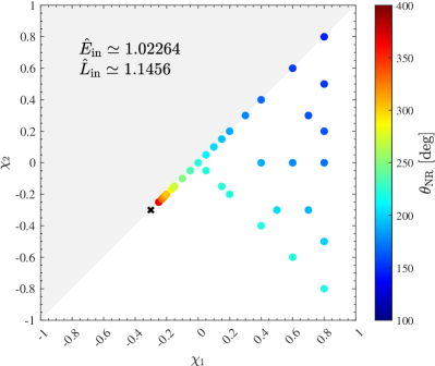
Figure 2: NR scattering angles for equal-mass simulations with $\hat{E}_{\rm in}\simeq 1.02264$ and $\hat{L}_{\rm in}\simeq 1.1456$ against individual spin variables. This figure shows (see the color code) that the angles essentially depend only on the sum of the spins.

III NR-deduced physical observables

In this section, we discuss some observables that can be directly extracted from the NR simulations presented in Sec. II above by using only minimal analytical assumptions.

III.1 Critical orbital angular momentum $L_{0}$ in nonspinning scattering

We define the critical (canonical) angular momentum $L_{0}$ of nonspinning binaries as the value marking the boundary between scattering and plunging systems. Several works (both analytical Eardley and Giddings (2002); Yoshino and Nambu (2003); Giddings and Rychkov (2004); Amati et al. (2008); Damour (2018) and numerical Pretorius and Khurana (2007); Shibata et al. (2008); Sperhake et al. (2009, 2013); Damour and Rettegno (2023)) have investigated the value of $L_{0}$ (and the subtleties in defining it in view of the importance of radiation losses).

Here we follow Ref. Damour and Rettegno (2023) in estimating $L_{0}$ by fitting the sequence of NR scattering angles at fixed energy using a template expected to capture the singular behavior of $\theta(L)$ as $L\to L_{0}^{+}$. Namely, we use (recalling the notation $\hat{L}\equiv L/M^{2}$)

$$\theta_{\rm NR}^{\rm fit}(\hat{L})=\frac{\hat{L}}{\hat{L}_{0}}\ln\left(\frac{1}{1-\hat{L}_{0}/\hat{L}}\right)\left[\hat{\chi}_{\rm 3PM}(\hat{L};\hat{L}_{0})+2\frac{a_{4}}{\hat{L}^{4}}\right]\,,$$ (7)

where $\hat{\chi}_{\rm 3PM}(\hat{L};\hat{L}_{0})$ is a third order polynomial in $1/\hat{L}$ defined so as to ensure a correct PM expansion up to 3PM, and where ${a_{4}}$ is a 4PM-level fitting parameter (see Sec. VI A of Ref. Damour and Rettegno (2023) for details).

For the lower-energy simulations ($\hat{E}_{1}=1.02264$), we could improve the estimate of $L_{0}$ computed in Ref. Damour and Rettegno (2023) and get

$$\hat{L}_{0}^{\rm fit}(\hat{E}_{1}) =1.0787\pm 0.00028\,,$$

$$a_{4}^{\rm fit}(\hat{E}_{1}) =6.78\pm 0.50\,,$$ (8)

The corresponding estimate of $\hat{L}_{0}^{\rm fit}(\hat{E}_{1})$ in Damour and Rettegno (2023) is $\hat{L}_{0}^{\rm fit}(\hat{E}_{1})=1.0773$ .

Instead, for the higher-energy ones ($\hat{E}_{2}=1.04033$ and $\hat{E}_{3}=1.05548$, respectively corresponding to center-of-mass velocities $v_{\rm cm,2}\simeq 0.2757$ and $v_{\rm cm,3}\simeq 0.3199$), we got

$$\hat{L}_{0}^{\rm fit}(\hat{E}_{2}) =1.15305\pm 0.00029\,,$$

$$a_{4}^{\rm fit}(\hat{E}_{2}) =12.83\pm 0.81\,;$$ (9)

and

$$\hat{L}_{0}^{\rm fit}(\hat{E}_{3}) =1.21431\pm 0.00036\,,$$

$$a_{4}^{\rm fit}(\hat{E}_{3}) =20.2\pm 1.8\,.$$ (10)

In Fig. 3 we display these numerical estimates against $v_{\rm cm}$. Note that the two new values $\hat{L}_{0}^{\rm fit}(\hat{E}_{2})$ and $\hat{L}_{0}^{\rm fit}(\hat{E}_{3})$ fill a gap in the previous knowledge of the critical $\hat{L}_{0}$ for intermediate energies. Figure 3 also displays the critical angular momentum estimates obtained through the high-velocity simulations of Refs. Shibata et al. (2008); Sperhake et al. (2009). We compare these to analytical estimates based on using the EOB transcription of PM scattering results ($w^{eob}$ nPM). For more details on these, see Sec. IV of Ref. Damour and Rettegno (2023).

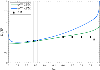
Figure 3: Comparison between the critical (rescaled) orbital angular momentum $L_{0}/E^{2}$ extracted from NR simulations and various analytical predictions. The three leftmost NR data points correspond to our fitted estimates [Eqs. (III.1)-(III.1)]. The first point updates the estimate of Ref. Damour et al. (2014b), while the other two (highlighted by a vertical grey line) explore a new velocity interval. The five points on the right correspond to the high-energy simulations of Refs. Shibata et al. (2008); Sperhake et al. (2009). We also display, for comparison, some EOB-PM predictions.

We can also compare the fitted values $a_{4}^{\rm fit}(\hat{E}_{n})$, $n=1,2,3$, or more precisely the corresponding 4PM scattering coefficient, $\theta_{4}^{\rm fit}(\hat{E}_{n})$, to the recently determined (radiation-reacted) analytical value of the function $\theta_{4}(\hat{E})$ Bern et al. (2022); Dlapa et al. (2022a, 2023); Bini et al. (2023). We find $\theta_{4}^{\rm fit}(\hat{E}_{1})\simeq 60.66$ [to be compared to $\theta_{4}^{\rm analyt}(\hat{E}_{1})=58.16$], as well as $\theta_{4}^{\rm fit}(\hat{E}_{2})\simeq 84.93$ [to be compared to $\theta_{4}^{\rm analyt}(\hat{E}_{2})=77.07$] and $\theta_{4}^{\rm fit}(\hat{E}_{3})\simeq 109.23$ [to be compared to $\theta_{4}^{\rm analyt}(\hat{E}_{3})=94.34$].

When considering spinning systems, the critical curve $L_{0}/E^{2}=F(\hat{E})$ becomes a critical surface $L_{0}/E^{2}=F(\hat{E},\chi_{1},\chi_{2})$. In the following subsection we show how to obtain one point on this critical surface.

III.2 Spin dependence of the scattering angle

We now focus on the spinning simulations and try to determine from our NR results (with minimal analytical assumptions) the spin dependence of the scattering angle at fixed initial energy and angular momentum. The color coding of Fig. 2 makes it apparent that the scattering angle mainly depends on the sum of the spins, i.e. is nearly constant along the lines $\chi_{1}+\chi_{2}=cst$. In particular, the simulations with opposite spins ($\chi_{1}=-\chi_{2}$, i.e. the second diagonal in Fig. 2) all lead to scattering angles $\theta_{\rm NR}$ very close (within the percent level) to the nonspinning one at the center. This numerical result corresponds to the well-known analytical fact (see, e.g., Damour (2001)) that the leading-PN value of the linear-in-spin interaction potential (spin-orbit) depends on the effective spin ${\bf S}_{\rm eff}=[1+3m_{2}/(4m_{1})]{\bf S}_{1}+[1+3m_{1}/(4m_{2})]{\bf S}_{2}$, while the leading-PN value of the spin-spin interaction potential depends on ${\bf S}_{0}=(1+m_{2}/m_{1}){\bf S}_{1}+(1+m_{1}/m_{2}){\bf S}_{2}$. In the equal-mass case considered here, this means that the two leading-order spin-dependent interactions only depend on the total spin ${\bf S}_{\rm tot}={\bf S}_{1}+{\bf S}_{2}$, and therefore only on $\chi_{1}+\chi_{2}$ in the spin-aligned case. We have found that this property remains true to a very good approximation, much beyond the leading-order PN approximation. As we will describe below, we have derived a high-PM-accuracy Hamiltonian incorporating the state of the art analytical knowledge of PM gravity, and we found (as displayed in Table 5 in Appendix C) that the averaged scattering angle of two (equal-mass) spinning BHs is analytically predicted to depend essentially only on the average spin $\chi_{+}\equiv\frac{1}{2}(\chi_{1}+\chi_{2})$.

Let us also recall that the spin-orbit interaction term

$$H_{\rm SO}\simeq+\frac{2G}{c^{3}r^{3}}{\bf L}\cdot{\bf S}_{\rm eff}$$ (11)

is repulsive (respectively, attractive) for spins parallel (respectively, antiparallel) to the orbital angular momentum ${\bf L}$. This fact has a strong effect on the last stable orbits of quasi-circular spinning binaries (e.g., Damour (2001); Campanelli et al. (2006b)). In the present, scattering situation, it implies that the leading-order spin-dependent contribution to the scattering angle is negative (positive) when ${\bf L}\cdot{\bf S}_{\rm eff}>0$ (${\bf L}\cdot{\bf S}_{\rm eff}<0$), see e.g. Bini and Damour (2017a). This leading-order PN analytical prediction holds also true for the predictions from the PM-accurate EOB Hamiltonian derived below, as can be seen in the results displayed in Table 6 in Appendix C.

Our numerical results (displayed in Fig. 2) agree remarkably well with the analytical expectation that the (average) scattering angle depends essentially on the average spin,

$$\chi_{+}\equiv\frac{1}{2}(\chi_{1}+\chi_{2})\,,$$ (12)

with only a weak dependence on the antisymmetric spin combination

$$\chi_{-}\equiv\frac{1}{2}(\chi_{1}-\chi_{2})\,.$$ (13)

In particular, the numerical results displayed in Table II show that, for most of the (half) spin differences explored by our simulations, the dependence of $\theta_{\rm NR}\equiv\frac{1}{2}(\theta_{1}+\theta_{2})$ on $\chi_{-}$ stays within the numerical uncertainty with which we could determine $\theta_{\rm NR}$. For instance, even when $\chi_{-}=0.80$, Table II reports that the difference between $\theta_{\rm NR}(\chi_{1}=0,\chi_{2}=0)=221.823^{+0.762}_{-0.002}$ and $\theta_{\rm NR}(\chi_{1}=0.80,\chi_{2}=-0.80=221.679^{+0.489}_{-0.002}$ is only $0.144\pm 0.454$. In view of this finding, the present limited precision of our numerical results does not allow us to meaningfully extract any reliable estimate of the dependence of the function $\theta_{\rm NR}(\chi_{+},\chi_{-})$ on $\chi_{-}$. [We note in passing that, for the equal-mass systems we are considering, the relative (i.e. average) scattering angle $\theta_{\rm rel}=\frac{1}{2}(\theta_{1}+\theta_{2})$ is a symmetric function of $\chi_{1}$ and $\chi_{2}$, and therefore an even function of $\chi_{-}$.]

On the other hand, if we focus (for maximum accuracy) on the equal-spin subset of our numerical results ($\chi_{1}=\chi_{2}$, so that $\chi_{+}=\chi_{1}=\chi_{2}$ and $\chi_{-}=0$), we can fit our results to various possible analytical templates so as to extract a numerical estimate of the univariate function $\theta_{\rm NR,eq}(\chi_{+})=\theta_{\rm NR}(\chi_{+},\chi_{-}=0)$. Removing the $(\chi_{1}=\chi_{2}=-0.17)$ data point (which stood out as an outlier compared to its neighbouring data points in all our fits; see also Fig. 6), we found that we could fit within numerical errors the remaining eighteen equal-spin data points to the following simple five-parameter template:

$$\theta_{\rm NR,eq}^{\rm fit}(\chi_{+})= \,\frac{1-{\rm ln}\left(\chi_{+}-\chi_{+}^{\rm crit}\right)}{1-{\rm ln}\left(-\chi_{+}^{\rm crit}\right)}$$

$$\times\left(\theta_{0}+\theta_{1}\,\chi_{+}+\theta_{2}\,\chi_{+}^{2}+\theta_{3}\,\chi_{+}^{3}\right)\,.$$ (14)

Note that this template incorporates a logarithmic singularity at some critical spin $\chi_{+}^{\rm crit}$. This singularity models the image on the $\chi_{+}$ axis of the logarithmic singularity generically expected when crossing the border between scattering and coalescence Damour and Rettegno (2023). We find the best-fit values (when measuring angles in radians) to be

$$\theta_{0} =3.8748\pm 0.0017\,,$$

$$\theta_{1} =1.881\pm 0.018\,,$$

$$\theta_{2} =0.43\pm 0.10\,,$$

$$\theta_{3} =1.07\pm 0.13\,,$$

$$\chi_{+}^{\rm crit} =-0.2932\pm 0.0013\,,$$ (15)

leading to a satisfactory reduced chi-squared: $\chi^{2}/(18-5)\simeq 0.63$.

The successful fit of our numerical results to the template (III.2) allows us to meaningfully extract from our NR results an estimate of the critical value of $\chi_{+}$ (at least in the equal-spin case) leading to immediate plunge rather than scattering. Indeed, the value $\chi_{+}^{\rm crit}=-0.2932\pm 0.0013$ formally corresponds to an infinite scattering angle. This result completes the critical values of $L_{0}$ displayed in Fig. 3 by yielding the numerical estimate of one point on the surface $L_{0}^{\rm crit}/E^{2}=F(\hat{E},\chi_{1},\chi_{2})$ describing the critical initial data for spinning BBHs leading to immediate coalescence, namely the point

$$L_{0}^{\rm crit}/E^{2}=1.0953,\,\hat{E}=1.02264,\,\chi_{1}=\chi_{2}=-0.2932\,.$$ (16)

The computations above have been based on the relative scattering angle $\theta_{\rm rel}=\frac{1}{2}(\theta_{1}+\theta_{2})$. We leave to future work a NR-based study of the dissymmetry between $\theta_{1}$ and $\theta_{2}$ linked to asymmetric-spin recoil effects.

IV PM-based analytical predictions

In this section, we compare the NR data presented in Sec. II to analytical PM results for the scattering angle of a BBH system on hyperbolic orbits. For nonspinning BHs, these terms are known up to 4PM, including radiation-reaction effects Bern et al. (2022, 2021a); Dlapa et al. (2022b); Manohar et al. (2022); Dlapa et al. (2023); Bini et al. (2023). The PM formalism has also been extended to include spinning objects, with PM accuracies depending on the order in spin  Bini and Damour (2017b, 2018); Vines (2018); Vines et al. (2019); Guevara et al. (2019b); Kälin and Porto (2020b); Kosmopoulos and Luna (2021); Chen et al. (2022); Aoude et al. (2022); Jakobsen and Mogull (2022); Bern et al. (2021b, 2023); Febres Cordero et al. (2023); Alessio and Di Vecchia (2022); Alessio (2023).

IV.1 Post-Minkowskian expanded scattering angles

In the nonspinning limit, the PM approximation (which is a power series in the gravitational constant $G$) translates to a power series in $1/\ell$, where $\ell$ denotes the rescaled orbital angular momentum,

$$\ell=\frac{L}{G\mu M}\,.$$ (17)

The total (nonspinning) scattering angle up to $n$PM order (included) can then be written as

$$\theta_{n{\rm PM}}^{\rm orb}(\gamma,\ell)\equiv\sum_{k=1}^{n}2\frac{\theta_{k}^{\rm orb}(\gamma)}{\ell^{k}}\,,$$ (18)

where $\gamma$ denotes the Lorentz factor between the two incoming worldlines. We recall that $\gamma$ is equal to the rescaled EOB effective energy, $\gamma=E^{\rm eob}_{\rm eff}/\mu$, which is related to the (real) total energy of the system by

$$\gamma=\frac{E^{2}-m_{1}^{2}-m_{2}^{2}}{2m_{1}m_{2}}\,.$$ (19)

When considering spinning BHs, the PM expansion is modified because of the spin-induced multipolar structure of BHs. More precisely, the multipolar structure of Kerr black holes is polynomial in the Kerr parameters $a_{i}=S_{i}/m_{i}$ (with dimension of length), so that each spin-order, $O(S^{m})$ involves a $m$-th order polynomial in $a_{1}$ and $a_{2}$. In the current PM literature on spinning bodies, it is usual to consider the Kerr parameters (or “ring radii”) $a_{i}$, as expansion parameters independent of the basic PM expansion parameters $Gm_{1}$, $Gm_{2}$. In other words, one uses a double expansion in powers of $Gm_{i}$ (PM expansion), and in powers of $a_{i}$ (spin expansion). This leads to a double counting $(n,m)$, in which the PM order $n$ counts the (sum of the) powers of $Gm_{i}$, while $m$ counts the (sum of the) powers of $a_{i}$. However, one must remember that we are interested in the dynamics of spinning BH’s for which we have the inequality $a_{i}\leq Gm_{i}$. Therefore, a term of order $(Gm)^{n}a^{m}$ is of real PM order $n+m$. This issue must be kept in mind, and will come back in our discussion below, but, for compatibility with the literature, we will continue to refer to a term of order $(Gm)^{n}a^{m}$ as being formally of $n$-PM order.

The natural dimensionless expansion parameters associated with the PM and spin expansions are $Gm_{i}/b$ and $a_{i}/b$ where $b$ denotes the impact parameter. We will, instead of $b$, use the (rescaled) angular momentum $\ell\equiv L/(Gm_{1}m_{2})$, with $L=P_{\rm cm}b$. We also utilize $S_{i}=m_{i}a_{i}$ as spin variables, so that each spin order will be identified by a corresponding power of $S_{i}/\ell$. One then writes the combined PM, and spin, expansion of the scattering angle as (in the spin-aligned case)

$$\theta_{n{\rm PM}}(\gamma,\ell,S_{i})\equiv\sum_{k=1}^{n}2\frac{\theta_{k}(\gamma,\ell,S_{i})}{\ell^{k}}\,,$$ (20)

with the $k$PM contribution to the scattering angle, $\theta_{k}(\gamma,\ell,S_{i})$, being further expanded in spin powers, namely

$$\theta_{k}(\gamma,\ell,S_{i})\equiv\sum_{m\geq 0}\frac{\theta^{\rm S^{m}}_{k}(\gamma)}{\ell^{m}}\,.$$ (21)

Here, $\theta^{\rm S^{m}}_{k}(\gamma)$ denotes a homogeneous polynomial in the two spins of order $m$. For instance

$$\theta^{\rm S}_{k}(\gamma)=\theta^{\rm S_{1}}_{k}(\gamma)S_{1}+\theta^{\rm S_{2}}_{k}(\gamma)S_{2}\,,$$ (22)

$$\theta^{\rm S^{2}}_{k}(\gamma)=\theta^{\rm S_{1}^{2}}_{k}(\gamma)S_{1}^{2}+\theta^{\rm S_{1}S_{2}}_{k}(\gamma)S_{1}S_{2}+\theta^{\rm S_{2}^{2}}_{k}(\gamma)S_{2}^{2}\,.$$ (23)

As several theoretical papers on spinning scattering use as basic variables covariantly-defined impact parameters, spins and orbital angular momentum (say $L_{\rm cov}$), while we work here with the canonically-defined orbital angular momentum ($L\equiv L_{\rm can}$), we need to recall the connection between $L_{\rm cov}$ and $L\equiv L_{\rm can}$. In the spin-aligned case, it is simply given by using the relation Vines (2018)

$$J=L_{\rm can}+m_{1}a_{1}+m_{2}a_{2}=L_{\rm cov}+E_{1}a_{1}+E_{2}a_{2}\,,$$ (24)

where $a_{i}=S_{i}/m_{i}$ and $E_{i}=\sqrt{m_{i}^{2}+P_{\rm c.m.}^{2}}$. In order to obtain the coefficients $\theta_{k}^{\rm S^{m}}$ of the double PM- and spin-expansion as functions of the canonical orbital angular momentum, we transform $L_{\rm cov}$ into $L_{\rm can}$ using Eq. (24), re-expand in powers of spin, and neglect higher-order contributions.

In the following, when considering spinning systems, we include: (i) nonspinning contributions up to 4PM (including radiation-reaction effects) Bern et al. (2021a); Bini et al. (2021); Herrmann et al. (2021); Manohar et al. (2022); Dlapa et al. (2023); Bini and Damour (2022); (ii) quadratic-in-spin terms up to the 3PM order (including radiation-reaction effects) Jakobsen and Mogull (2022); (iii) cubic and fourth order in spin effects up to the 2PM order Guevara et al. (2019a). In addition, as during the development of this work the conservative Jakobsen et al. (2023a), and radiative Jakobsen et al. (2023b), linear-in-spin contributions have been computed at the 4PM level, we also incorporated these new analytical results. Their impact is separately discussed below.

IV.2 $w^{eob}$ resummed scattering angles

In addition to PM-expanded scattering angles, we also compute $w^{eob}$-resummed PM angles, as introduced in Ref. Damour and Rettegno (2023) and generalized here to spinning bodies.

Let us briefly introduce the EOB formalism (see, e.g., Sec. IIB of Ref. Damour and Rettegno (2023) for more details). The EOB framework Buonanno and Damour (1999, 2000); Damour et al. (2000) is a way of mapping the general-relativistic dynamics of two masses $m_{1},m_{2}$ (considered in the center-of-mass system) onto the effective relativistic dynamics of a single body of mass $\mu=m_{1}m_{2}/(m_{1}+m_{2})=\nu M$. The “real” center-of-mass Hamiltonian is related to the “effective” one through

$$H_{\rm real}=M\sqrt{1+2\nu\left(\frac{H_{\rm eff}}{\mu}-1\right)}\,.$$ (25)

For scattering motions, the value of the effective energy $E_{\rm eff}=H_{\rm eff}$ is simply related to the Lorentz factor $\gamma=-u_{1}\cdot u_{2}$ between the two incoming worldlines by $E_{\rm eff}=\mu\gamma$. This implies that the total ADM energy of the system is related to $\gamma$ via

$${\hat{E}}=\frac{E}{M}=\sqrt{1+2\nu(\gamma-1)}\,.$$ (26)

The effective Hamiltonian $H_{\rm eff}$ is obtained by solving (in $P_{0}=-H_{\rm eff}$) some relativistic-like mass-shell condition of the general form

$$0=\mu^{2}+g_{\rm eff}^{\mu\nu}P_{\mu}P_{\nu}\,,+Q(R,P_{\mu})\,$$ (27)

where $Q(R,P_{\mu})$ gathers terms more than quadratic in $P_{\mu}$. When considering scattering problems, it is convenient to use a mass-shell condition where the effective metric is the Schwarzschild metric, and where $Q(R,P_{\mu})$ is expressed as a function of the effective energy $-P_{0}=\mu\gamma$. Using isotropic coordinates, and rescaled variables, $\bar{r}=R/M$, $p_{\alpha}=P_{\alpha}/\mu$, the PM-expansion of the EOB mass-shell condition formally takes the form of a non-relativistic energy-conservation law, namely Damour (2018, 2020)

$$p_{\bar{r}}^{2}+\frac{\ell^{2}}{\bar{r}^{2}}=p_{\infty}^{2}+w^{eob}(\bar{r};\gamma)\,,$$ (28)

where $p_{\infty}=\sqrt{\gamma^{2}-1}$ and where the Newtonian-looking potential $w^{eob}(\bar{r};\gamma)$ [more precisely, $-w^{eob}(\bar{r})$] encapsulates the (relativistic, energy-dependent) attractive gravitational interaction. For nonspinning systems, the PM expansion of the $w^{eob}$ potential reads

$$w_{n{\rm PM}}^{\rm orb}(\bar{r},\gamma)=\sum_{k=1}^{n}\frac{w_{k}^{\rm orb}(\gamma)}{\bar{r}^{k}}\,,$$ (29)

where each order in $\frac{1}{\bar{r}}$ corresponds to the same PM order (e.g., the first term, $\frac{w_{1}^{\rm orb}(\gamma)}{\bar{r}}$, with $w_{1}^{\rm orb}(\gamma)=2(2\gamma^{2}-1)$, describes the 1PM gravitational interaction Damour (2016)).

For aligned-spin binaries we can generalize Eq. (29) simply by considering a spin-dependent radial potential of the form (up to fourth order in the spins)

$$w_{n{\rm PM}}(\bar{r},\gamma,\ell,S_{i}) =w^{\rm orb}(\bar{r},\gamma)$$

$$+\frac{\ell\,w_{n{\rm PM}}^{\rm S}(\bar{r},\gamma)}{\bar{r}^{2}}+\frac{w_{n{\rm PM}}^{\rm S^{2}}(\bar{r},\gamma)}{\bar{r}^{2}}$$

$$+\frac{\ell\,w_{n{\rm PM}}^{\rm S^{3}}(\bar{r},\gamma)}{\bar{r}^{4}}+\frac{w_{n{\rm PM}}^{\rm S^{4}}(\bar{r},\gamma)}{\bar{r}^{4}}.$$ (30)

Here each $w_{n{\rm PM}}^{\rm S^{m}}(\bar{r},\gamma)$ is a polynomial of order $m$ in spins, whose coefficients admit an expansion in powers of $\frac{1}{\bar{r}}$ up to the order $\frac{1}{\bar{r}^{n}}$ included. For instance, we have (at spin orders $m=1$ and $m=2$)

$$w_{n{\rm PM}}^{\rm S}(\bar{r},\gamma)=\sum_{k=1}^{n}\frac{w_{k}^{\rm S_{1}}(\gamma)S_{1}+w_{k}^{\rm S_{2}}(\gamma)S_{2}}{\bar{r}^{k}}\,,$$ (31)

$$w_{n{\rm PM}}^{\rm S^{2}}(\bar{r},\gamma)=\sum_{k=1}^{n}\frac{w_{k}^{\rm S_{1}^{2}}(\gamma)S_{1}^{2}+w_{k}^{\rm S_{1}S_{2}}(\gamma)S_{1}S_{2}+w_{k}^{\rm S_{2}^{2}}(\gamma)S_{2}^{2}}{\bar{r}^{k}}\,.$$ (32)

The energy-dependent $w^{*}_{k}(\gamma)$ coefficients entering the EOB potentials are in 1-to-1 correspondence with the $\theta^{*}_{k}(\gamma)$ coefficients of the scattering angle expansion. These relations can be found by expanding, and solving, at each order in $G$ and in spin, the following equation

$$\pi+ \theta\left(\gamma,\ell,S_{i}\right)=-2\int_{\bar{r}_{\rm min}}^{+\infty}d\bar{r}\,\frac{\partial p_{\bar{r}}\left(\bar{r},\gamma,\ell,S_{i}\right)}{\partial\ell}$$

$$\quad=\int_{\bar{r}_{\rm min}}^{+\infty}\frac{d\bar{r}}{\bar{r}^{2}}\,\,\frac{2\ell-w^{\rm S}(\bar{r},\gamma)-w^{\rm S^{3}}(\bar{r},\gamma)/\bar{r}^{2}}{\sqrt{p_{\infty}^{2}-\ell^{2}/\bar{r}^{2}+w(\bar{r},\gamma,\ell,\chi_{i})}}\,.$$ (33)

Here $\bar{r}_{\rm min}$ denotes the turning point radius. The explicit equations linking the $\theta^{*}_{k}(\gamma)$ coefficients and the $w^{*}_{k}(\gamma)$ ones are given in Appendix B. When using the existing PM-expanded results for the scattering angle, the relations of Appendix B allow one to compute the explicit values of the PM-expansion coefficients $w^{*}_{k}(\gamma)$ describing the spin interactions within the EOB formalism. These values will be found in the ancillary file of this paper. Note that the so-constructed EOB potential is a function of the incoming energy and angular momentum of the system that incorporates both conservative and radiation-reaction effects.

Following Ref. Damour and Rettegno (2023), we then define spin-dependent $w^{eob}$-resummed scattering angles $\theta_{n{\rm PM}}^{w}(\gamma,\ell,S_{i})$ by substituting the $n$PM-accurate, spin-dependent, EOB potentials $w_{n{\rm PM}}(\bar{r},\gamma,\ell,S_{i})$ in Eq. (IV.2), without performing any expansion (in $G$ or in spin), i.e.

$$\pi+\theta^{w^{eob}}_{n{\rm PM}}\equiv\int_{0}^{\bar{u}_{\rm max}}d\bar{u}\,\frac{2\ell-w_{n{\rm PM}}^{\rm S}-w_{n{\rm PM}}^{\rm S^{3}}\,\bar{u}^{2}}{\sqrt{p_{\infty}^{2}-\ell^{2}\bar{u}^{2}+w_{n{\rm PM}}}}\,,$$ (34)

where we introduced $\bar{u}\equiv 1/\bar{r}$ and $\bar{u}_{\rm max}=1/\bar{r}_{\rm min}$.

V Comparing numerical results to analytical predictions

V.1 Numerics/analytics comparison for nonspinning simulations

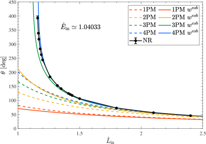
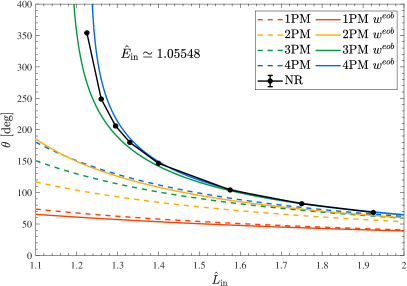
Figure 4: Comparison between NR scattering angles of nonspinning BBH systems and analytical PM predictions, both PM-expanded (dashed lines) and $w^{eob}$-resummed (solid lines). Left panel: Intermediate energy $\hat{E}_{\rm in}\simeq 1.04033$. Right panel: Higher energy $\hat{E}_{\rm in}\simeq 1.05548$. The $w^{eob}$-resummed 3PM and 4PM results show a remarkable agreement with numerical down to strong-field regimes.

We start by comparing, in Fig. 4, the results of the nonspinning NR simulations at fixed energy to both the PM-expanded, perturbative, predictions, Eq. (20), and their EOB-resummed versions, defined by Eq. (34). This comparison extends the one considered in Refs. Khalil et al. (2022); Damour and Rettegno (2023), which corresponded to the lower initial energy $\hat{E}_{1}$ used in Damour et al. (2014b) (see also Appendix C). The main findings of the latter comparison when considering the PM-expanded perturbative predictions remain true for the new, higher energies considered in this paper, $\hat{E}_{2}=1.04033$ and $\hat{E}_{3}=1.05548$. The sequence of PM-expanded results (dashed lines) monotonically approach, in an increasingly accurate way, the NR results in the high angular momenta domain (i.e., for relatively large impact parameters fields). However, they perform less and less well as the angular momentum decreases. Note, in particular, that, for our minimum $\hat{L}$, even the 4PM-accurate prediction differs by a factor $\gtrsim 2$ from the NR result.

On the other hand, the sequence of $w^{eob}$-resummed (PM-based) predicted angles (solid lines) perform much better than their perturbative counterparts. While the 1PM-based $w^{eob}$-resummed prediction is not better (and even slightly worse) than its perturbative analog, the 2PM-based $w^{eob}$-resummed fares as well as the 4PM perturbative one, and the 3PM and, especially, 4PM EOB-resummed results exhibit a remarkable agreement with NR data for essentially all orbital angular momenta. It should, however, be noted that the 4PM-based EOB-resummed predicted angles start to show visible discrepancies with NR results for the lowest $L$’s, especially for the highest energy $\hat{E}_{3}=1.05548$. More precisely, $w^{eob}_{\rm 4PM}$ somewhat overestimates the scattering angle, while $w^{eob}_{\rm 3PM}$ underestimates it. We discuss below how these findings can lead to NR-based ways of improving the knowledge of the exact $w^{eob}(\bar{r},\gamma)$ potential.

V.2 Extracting from NR results the gravitational interaction potential between nonspinning black holes

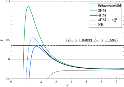
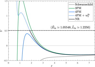
Figure 5: Comparison between the gravitational potential $V$ extracted from NR simulations and its EOB-PM equivalent. The Schwarzschild potential is plotted as a reference. Left panel: Intermediate energy $\hat{E}_{\rm in}\simeq 1.04033$. Right panel: Higher energy $\hat{E}_{\rm in}\simeq 1.05548$. In both cases, the angular momentum is set to the smallest values of angular momentum for which the system scattered. The horizontal lines mark the values of $p_{\infty}^{2}$ for each energy, determining the maximum point up to which it is possible to extract information about the numerical potential.

Having computed new suites of numerical simulations with higher initial energies, we can extend the strategy used in Sec. VIC of Ref. Damour and Rettegno (2023) and directly extract from the sequence of NR scattering angles (at a given energy) the NR radial potential $w_{\rm NR}(\bar{r})$ (in our chosen EOB coordinates). This extraction is done by iteratively using Firsov’s inversion formula Landau and Lifshitz (1960); Kälin and Porto (2020c) to invert the functional relation $w(\bar{r},\gamma)\to\theta(\ell,\gamma)$, Eq. (IV.2) (for nonspinning systems), i.e. to deduce the function $w_{\rm NR}(\bar{r})$ leading to the function $\theta_{\rm NR}(\ell)$, tabulated in Table 1 (for each fixed value of $\gamma$).

The so-extracted NR radial potential for the lower value $\gamma_{1}(E_{1})\simeq 1.09188$ has been displayed in Fig. 7 of Ref. Damour and Rettegno (2023). See Appendix C for an updated determination of $w_{\rm NR}(\bar{r},\gamma_{1})$. We focus here on the determination of the NR potentials $w_{\rm NR}(\bar{r},\gamma_{2})$ and $w_{\rm NR}(\bar{r},\gamma_{3})$ corresponding to the two higher-energy sequences of simulations reported in the present work. In addition, we compare the so-extracted NR gravitational potentials to their analytical counterparts, as defined by the PM-based EOB radial potential $w^{eob}(\bar{r},\gamma)$ defined in Eq. (29) above (for the nonspinning case).

Instead of plotting the various energy-dependent radial potentials $w^{*}(\bar{r},\gamma)$, it is useful to plot the corresponding “effective radial potentials”, completed by the additional centrifugal potential $+\frac{\ell^{2}}{\bar{r}^{2}}$. In other words, we shall compare the (Newtonian-like) effective potentials

$$V^{*}(\bar{r},\gamma,\ell)\equiv\frac{\ell^{2}}{\bar{r}^{2}}-w^{*}(\bar{r},\gamma)\,,$$ (35)

made by adding the (repulsive) centrifugal barrier term $\ell^{2}\,\bar{r}^{-2}$ to the (attractive) gravitational radial potential $-w^{*}(\bar{r},\gamma)$.

The comparison between $V^{\rm NR}(\bar{r},\gamma,\ell)$ and $V^{eob}_{n{\rm PM}}(\bar{r},\gamma,\ell)$ (for $n=3$ and $n=4$) is displayed in the two panels of Fig. 5. The left panel corresponds to the intermediate energy $\gamma_{2}(E_{2})\simeq 1.16456$, and uses the smallest NR orbital angular momentum leading to scattering, namely $\hat{L}\simeq 1.15950$ (corresponding to $\hat{b}_{\rm NR}=7.73$). The right panel corresponds to the higher energy $\gamma_{3}(E_{3})\simeq 1.22808$, and uses the smallest NR orbital angular momentum leading to scattering for that energy, namely $\hat{L}\simeq 1.22500$ (corresponding to $\hat{b}_{\rm NR}=7.00$). The NR-extracted potentials are determined only for (isotropic) radii larger than about $1.95$ (for $E_{2}$) and about $1.85$ (for $E_{3}$).

Note that, for both energies, the NR-extracted potential is very close to the 4PM-based EOB potential down to radii $\bar{r}\simeq 2.8$. However, in the interval $2\lesssim\bar{r}\lesssim 2.8$ $V^{eob}_{4{\rm PM}}(\bar{r})$ starts to exhibit visible differences with $V^{\rm NR}(\bar{r})$. For the intermediate energy $E_{2}$ the peak of $V^{eob}_{4{\rm PM}}$ lies just below the $p_{\infty}^{2}$ line, meaning that the EOB-4PM potential predicts a plunge instead of a scattering for this angular momentum and this energy. By contrast, the (less attractive) EOB-3PM potential still predicts scattering for this angular momentum and this energy. The situation is similar for the highest energy, $E_{3}$. In this case, the NR potential seems to interpolate between $V^{eob}_{4{\rm PM}}(\bar{r})$ and $V^{eob}_{3{\rm PM}}(\bar{r})$.

These results suggest that it would be useful to resum the EOB-PM potentials, so as to improve their performances at small radii. Leaving such an investigation to future work, we shall content ourselves here by exploring the effect of adding a formal, additional 5PM-level contribution $+\frac{w_{5}(\gamma)}{\bar{r}^{5}}$ to the analytically predicted 4PM EOB potential. We can use our determination of $w^{\rm NR}(\bar{r})$ to extract a best-fit value for the (energy-dependent) coefficient $w_{5}(\gamma)$. Fitting (for our three energies) $w^{\rm NR}(\bar{r},\gamma)$ to $w^{eob}_{4{\rm PM}}(\bar{r})+\frac{w_{5}(\gamma)}{\bar{r}^{5}}$ yields the following results:

$$w_{5}^{\rm fit}(\gamma_{1})= -1.00\pm 0.17\,,$$

$$w_{5}^{\rm fit}(\gamma_{2})= -2.16\pm 0.13\,,$$

$$w_{5}^{\rm fit}(\gamma_{3})= -3.47\pm 0.23\,.$$ (36)

Here the errors are indicative estimates obtained by applying the parametric inversion formulas to the confidence intervals defined by Eqs (III.1)$-$(III.1).

The negative sign (present at all energies) reflects the fact that the EOB-4PM potential is slightly too attractive at small radii (while the EOB-3PM potential is too repulsive for all radii). The strange behaviour of $V^{\rm fit}(\bar{r})=V^{eob}_{4{\rm PM}}(\bar{r})-\frac{w_{5}^{\rm fit}(\gamma)}{\bar{r}^{5}}$ at small radii, for the highest energy (right panel of Fig. 5) indicates that the addition of a (repulsive) 5PM term is only physically valid in a small range of radii (say in the range $2\lesssim\bar{r}\lesssim 2.8$). Indeed, when one uses a non-resummed potential, $w(\bar{r})=\frac{w_{1}}{\bar{r}}+\frac{w_{2}}{\bar{r}^{2}}+\cdots\frac{w_{n}}{\bar{r}^{n}}$, the last term determines the strong-field behavior. In particular, a negative 5PM term entails a (probably unphysical) repulsive core at very small radii. The use of suitably resummed versions of the EOB-PM potentials would probably avoid such undesirable features.

V.3 Comparing spinning simulations to analytical predictions (without 4PM spin-orbit terms)

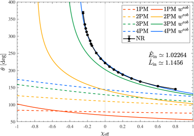
Figure 6: Scattering angle comparison between NR data and both the perturbative, and the EOB-transcribed, PM-based predictions for equal-mass, equal-spin simulations. The x-axis represents $\chi_{\rm eff}=\chi_{1}=\chi_{2}$. As in Fig. 4, we use dashed lines for the PM-expanded scattering angles, while the solid lines correspond to the $w^{eob}$-resummed ones. Similarly to the nonspinning case, the $w^{eob}$-resummed predictions are markedly more accurate, especially the 4PM-informed ones.

We now shift our attention to the suite of 35 NR simulations which computed the scattering angles of systems having many different spins, but with fixed initial energy ($\hat{E}_{\rm in}\simeq 1.02264$) and orbital angular momentum ($\hat{L}_{\rm in}=1.14560$). As we have already seen in Sec. III that the scattering angle mainly depends on the average spin $\chi_{+}$, we actually focus on the 19 simulations with equal spins (varying between $\chi_{1}=\chi_{2}=-0.30$ and $\chi_{1}=\chi_{2}=+0.80$) listed in Table 2.

In Fig. 6, we compare the equal-mass, equal-spin simulations to two types of PM-informed predictions: (i) standard PM-expanded angles, of the type of Eq. (20); and (ii) $w^{eob}$-resummed ones [see Eq. (34)]. In this section, we do not take into account the recently derived linear-in-spin (spin-orbit) 4PM results of Refs. Jakobsen et al. (2023a, b). In other words, we only use at the 4PM level (conservative and radiative) orbital effects. Since the analytical PM knowledge of the spin-dependent couplings varies with the spin order, we shall consider, for simplicity, only the following cases: (i) 1PM accuracy in all couplings up to quartic-in-spin terms (labelled as 1PM); (ii) 2PM accuracy in all couplings up to $S^{4}$ (labelled as 2PM); (iii) 3PM accuracy in the $(S^{0},S^{1},S^{2})$ couplings and 2PM accuracy in the $(S^{3},S^{4})$ ones (labelled as 3PM); and (iv) respectively (4PM,3PM,3PM,2PM,2PM) accuracy in the $(S^{0},S^{1},S^{2},S^{3},S^{4})$ couplings (labelled as 4PM).

A first conclusion one can draw from Fig. 6 is that PM-expanded results are rather unsatisfactory. Both the spin-averaged baseline and the spin-dependence are inaccurate, even for the highest PM accuracy. The agreement becomes, however, more satisfactory in the high-positive-spin domain, which involves (because of the repulsive effect of parallel spins) weaker-field interactions.

By contrast, the $w^{eob}$-resummed angles show, at each PM order, a systematically better agreement with NR data points, especially for the 4PM accuracy which exhibits a remarkable agreement.

V.4 Inclusion of 4PM spin-orbit terms

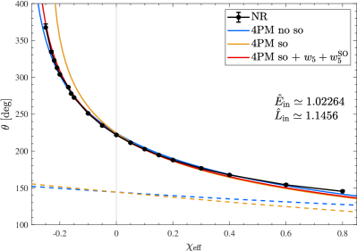
Figure 7: Effects due to the inclusion of the 4PM spin-orbit contributions Jakobsen et al. (2023a, b) to the scattering angle comparison of Fig. 6. Dashed lines correspond to PM-expanded scattering angles, while solid lines represent $w^{eob}$-resummed predictions. The blue curves contain spin-dependent terms up to 3PM and nonspinning contributions at 4PM (as in Fig. 6 above). The orange curves also incorporate (radiation-reacted) spin-orbit effects at 4PM level. Finally, the red line includes the two additional parameters $w_{5}$ and $w_{5}^{\rm SO}$ of Eqs. (37)-(V.4).

As already mentioned, conservative and radiative 4PM-level linear-in-spin contributions have been computed Jakobsen et al. (2023a, b) during the development of this work. We transformed the latter scattering-angle results into additional contributions to the 4PM EOB potential $w_{\rm 4PM}^{\rm S}$.

In Fig. 7 we compare the effect of incorporating the radiatively corrected 4PM spin-orbit terms (“4PM so”), to the 4PM-level angles computed in the previous section which only included orbital effects at 4PM (“4PM no so”). For simplicity, we do not separately consider here the conservative contribution to the 4PM spin-orbit terms.

Though the inclusion of 4PM spin-orbit terms has a relatively minor effect in the PM-expanded scattering angles (see dashed lines), their inclusion in $w_{\rm 4PM}^{\rm S}$ leads to much larger differences with respect to the corresponding 4PM-level EOB-resummed angles displayed in Fig. 6.

Looking at Fig. 7, it is clear that PM-expanded results remain rather unsatisfactory, and are significantly less accurate than $w^{\rm eob}$-resummed ones. However, the inclusion of 4PM-level spin-orbit effects in $w^{\rm eob}$ worsens the EOB-NR agreement that was obtained when only including 4PM-level orbital coefficients.

It is possible that the worsening due to the inclusion of 4PM spin-orbit terms is a signal pointing out the need to introduce some resummation of the spin-dependent $w_{\rm eob}^{\rm S}$ potential. [We recall that we are using here PM-expanded $w_{\rm eob}^{\rm S}$ potentials, as indicated in Eq. (IV.2).] However, the main cause of the worsening effect of the inclusion of 4PM spin-orbit terms might be the fact, recalled in Sec. IV above, that the nomenclature used in current spin-dependent PM works is physically inappropriate when dealing with spinning BHs. Indeed, because of the Kerr BH limit $a_{i}\leq Gm_{i}$, a term of formal $n$-PM order including the $m$-th power of spins is actually of $(n+m)$-PM order. Therefore, the additional spin-orbit contributions computed in Jakobsen et al. (2023a, b) are actually at the physical 5PM order. Similarly, the formally 2PM-level terms quartic in spins Guevara et al. (2019b) are actually at the physical 6PM order.

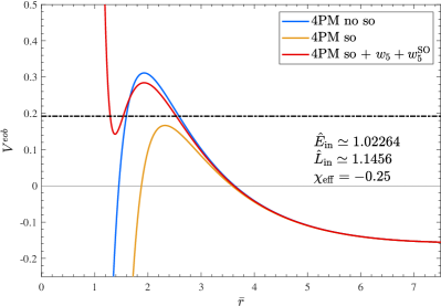
Figure 8: Comparison of various EOB-PM gravitational potentials $V^{eob}$ in the most negative spin case ($\chi_{\rm eff}=-0.25$), i.e. the leftmost NR point in previous figures. The displayed analytical potentials correspond to the solid lines in Fig. 7. The horizontal line marks the “energy level” $p_{\infty}^{2}$ defining the turning point of the EOB mass-shell condition, Eq. (28).

In view of the latter remark, we have explored the effect of including an additional spin-dependent term in $w^{\rm eob}$ belonging to the formal 5PM level, but to the physical 6PM level. For simplicity, we only considered a term involving a linear-in-spin contribution of the form

$$\Delta w^{\rm eob}=\frac{w_{5}}{{\bar{r}}^{5}}+\frac{w_{5}^{\rm SO}\,\ell\,\chi_{\rm eff}}{{\bar{r}}^{7}}\,.$$ (37)

This additional term contains two dimensionless parameters: (i) $w_{5}$, parametrizing an orbital 5PM-level contribution, and (ii) $w_{5}^{\rm SO}$, parametrizing a spin-orbit contribution at the physical 6PM level.

In view of our above finding that the purely orbital part of the EOB potential is slightly too attractive and needs to be completed by a $\frac{w_{5}(\gamma)}{{\bar{r}}^{5}}$ term, where $w_{5}(\gamma)$ is an energy-dependent negative coefficient, we fix its value to $w_{5}^{\rm fit}(\gamma_{1})$, Eq. (V.2), as the incoming energy of our spinning simulations corresponds to $\hat{E}_{1}\equiv\hat{E}(\gamma_{1})$. Concerning the second, spin-orbit-related, parameter $w_{5}^{\rm SO}$ in Eq. (37), we determine it by imposing that the corresponding effective Newtonian-like potential $V^{eob}$, Eq. (35), predicts immediate coalescence for the critical value $\chi_{\rm crit}=-0.2932\pm 0.0013$, Eq. (III.2), obtained above by fitting numerical results to the simple template of Eq. (III.2). This fixes the two parameters entering Eq. (37) to the approximate values

$$w_{5} =-1.00\pm 0.17\,,$$

$$w_{5}^{\rm SO} =+17.3\pm 0.6\,.$$ (38)

The corresponding $w^{eob}$-resummed scattering angles computed using the (central) values of Eq. (V.4) are displayed in Fig. 7 as a red curve (labelled “4PM so + $w_{5}+w_{5}^{\rm SO}$”). The addition of the term $\Delta w^{\rm eob}$, Eq. (37), leads to a better visual agreement between NR and EOB, at least for negative spins (on the large positive spin side, it slightly worsens the NR-EOB difference).

In order to better understand the physical origin of the differences between the various 4PM-level curves displayed in Fig. 7, we plot in Fig. 8 the corresponding Newtonian-like effective potentials $V^{eob}$, Eq. (35). Let us recall the meaning of the labels in Fig. 7: (i) “4PM no so” refers to a potential including (radiation-reacted) 4PM orbital effects without including any spin-orbit contributions at 4PM; (ii) “4PM so” additionally includes 4PM radiatively-corrected spin-orbit terms Jakobsen et al. (2023b); and finally (iii) “4PM so + $w_{5}+w_{5}^{\rm SO}$” differs from “4PM so” by including the potential $\Delta w^{\rm eob}$, Eq. (37), with the (central) values of Eq. (V.4). The dash-dotted horizontal line corresponds to the value of $p_{\infty}^{2}$, which defines the turning point of the EOB mass-shell condition, Eq. (28).

The vertical distance between “4PM no so” (blue line) and “4PM so” (orange line) measures the effect of the (radiation-reacted) 4PM spin-orbit contribution. The inclusion of these terms leads to a more attractive potential. Actually, the corresponding potential is now below the $p_{\infty}^{2}$ “energy level” which means that the system is predicted to no longer scatter but to plunge (in agreement in Fig. 7).

The $\Delta w^{\rm eob}$ correction makes the potential (red line) more repulsive. This leads to a turning point around $\bar{r}\simeq 2.5$ and to a finite scattering angle. This corrected potential also includes a (probably unphysical) repulsive core around $\bar{r}\simeq 1$.

At this stage, the meaning of these results is unclear. One will need to explore more values of the incoming energy, of the incoming angular momentum, and of the spins to assess whether it is indeed necessary to add (energy-dependent) terms, such as Eq. (37), to the current best analytical knowledge of the EOB potential.

VI Discussion

In this paper we presented numerical simulations of the scattering of equal-mass BBHs using the Einstein Toolkit et al. (2022).

We first computed three sequences of equal-mass, nonspinning BBHs at fixed initial energy and varying angular momentum. The first sequence, with initial energy $\hat{E}_{\rm in,1}\simeq 1.02264$, reproduces and extends the results of Ref. Damour et al. (2014b). These served as a useful cross-check against previous simulations performed with different numerical codes. They were also used to improve the estimate of the critical angular momentum $L_{0}$, marking the boundary between scattering and plunging systems. We then computed two other sequences of simulations at higher energies, $\hat{E}_{\rm in,2}\simeq 1.04033$ and $\hat{E}_{\rm in,3}\simeq 1.05548$, probing stronger-field regimes. These two series allowed us to compute the critical angular momentum $L_{0}$ in previously unexplored regions of center-of-mass velocities, $v_{\rm cm,2}\simeq 0.2757$ and $v_{\rm cm,3}\simeq 0.3199$. This leaves as regions not yet covered by NR simulations of nonspinning BHs the low velocity regime, $v_{\rm cm}\lesssim 0.2$, and the intermediate velocity one, $v_{\rm cm}\simeq 0.3-0.6$.

We then presented, for the first time, a suite of numerical simulations of equal-mass aligned-spins BHs. For these, we fixed both initial energy and angular momentum to be $(\hat{E}_{\rm in},\hat{L}_{\rm in})\simeq(1.02264,1.1456)$ and varied the individual spins in the range $-0.3<\chi_{i}<0.8$. We found (as expected both from NR simulations of coalescing binaries and from analytical predictions) the spin interaction to depend mainly on the total spin. We extracted from numerical data the coefficients of the linear and quadratic spin dependence of the scattering angle at the considered energy and angular momentum.

We compared our numerical results to PM-based predictions for the scattering angles of equal-mass BHs. We used two types of PM-based analytical predictions: (i) usual, perturbative PM-expanded results, see Eq. (20); and (ii) a transcription of PM results within the EOB formalism using a (spin-dependent, radiation-reacted) radial potential in isotropic (EOB) gauge, $w^{eob}(\bar{r},L,S_{1},S_{2})$, see Eq. (34). We found that PM-expanded scattering angles exhibit (both for nonspinning and spinning systems) an acceptable agreement with NR data only for large impact parameters, consistently with the PM framework being a weak-field expansion. On the contrary, a transcription of the PM information into a corresponding (energy-dependent, radiation-reacted, spin-dependent) EOB gravitational potential $w^{eob}(\bar{r},L,S_{1},S_{2})$ yields remarkable improvements in the scattering angle comparisons, especially when using the highest available PM accuracy. See Figs. 4 and 6. In the case of spinning simulations, we found that the inclusion of the recently computed 4PM-level spin-orbit contribution worsened the remarkable agreement (displayed in Fig. 6) between NR angles and the EOB-resummed 4PM-level ones (without 4PM spin-orbit terms). See Fig. 7.

Visible discrepancies between NR results and EOB-PM-predicted ones occur only for the few nonspinning cases where the impact parameter is close to the critical one leading to plunge rather than scattering and, for spinning simulations, when including the 4PM-level spin-orbit contributions. See Fig. 5, where we compare (for nonspinning systems) the EOB-PM potential to a corresponding potential directly extracted from the NR scattering data by inverting the relation: potential $\to$ scattering angle. We could, however, improve the accuracy of the EOB-PM gravitational potential by adding (an NR-fitted) additional (energy-dependent) 5PM-level contribution $w^{\rm fit}_{5}(\gamma)/\bar{r}^{5}$, see Eq. (V.2). Similarly, in the spinning case, we could improve the NR-EOB match obtained when incorporating the 4PM-level radiation-reacted spin-orbit terms by including an additional (formally) 5PM-level contribution including a spin-orbit term, Eqs. (37) and (V.4). The sensitivity of the dynamics to spin-dependent contributions at the 4PM level is studied in Fig. 8.

The present work can be extended in several directions. On the numerical side, a more thorough exploration of the parameter space is called for, notably by considering different energies, mass ratios, and spin orientations. In addition, it would be useful to complete the computation of the scattering angles by accurately estimating the emitted waveform, and by numerically estimating the corresponding radiative losses of energy, linear momentum and angular momentum.

On the analytical side, one should explore possible resummations of the EOB-PM radial potential, and generalize it to the non-aligned-spin case. It would also be interesting to explore other possible EOB reformulations of perturbative PM results, e.g. using different EOB gauges. Finally, when having in hands NR waveforms, one should compare them to the recent analytical computations of $O(G^{3})$-accurate, PM-expanded waveforms Brandhuber et al. (2023); Herderschee et al. (2023); Georgoudis et al. (2023).

Despite the above-mentioned limitations, we hope that the results presented here will offer a useful starting point for constructing accurate waveform models for spinning BHs in eccentric and hyperbolic motions, by combining information from NR and PM data within an EOB framework.

Appendix A Numerical Relativity Systematics

A.1 Impact of NR Resolution

One aspect of our numerical setup that can affect accuracy is the spatial resolution of the simulations. In order to test the robustness of the scattering angle to the NR resolution, we choose a fiducial binary and repeat the scattering simulation at three different resolutions, $N=\left[64,72,80\right]$. Here $N$ denotes the number of grid points on the finest level such that the resolution of the smallest box around the puncture is $\sim 2m_{p}/N$, with $N=64$ denoting the lowest resolution and $N=80$ the highest. Here we take a nonspinning configuration with $P_{\rm ADM}=0.15$ and $b_{\rm NR}=10.0$. As shown in Fig. 9, we find that the choice of resolution has a minimal impact on the scattering angle, with the errors due to finite NR resolution being subdominant to the errors from the polynomial extrapolation. A summary is given in Table 3.

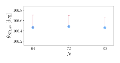
Figure 9: Error on the average scattering angle $\theta_{\rm NR,av}$ derived from the numerical relativity simulations for three different resolutions on the finest grid. Here, $N=80$ represents the highest resolution, and default choice, whereas $N=64$ denotes the lowest resolution. For all three resolutions, the upper errors are set by lower-order polynomial fits that overestimate the scattering angle. The lower error bars are set by high-order polynomials that manifestly agree with the preferred order.

Table 3: A set of equal-mass, nonspinning simulations with an initial momentum $P_{\rm ADM}=0.175$ and different resolutions.

$N$	$\hat{b}_{\rm NR}$	$\hat{E}_{\rm in}^{\rm{ADM}}$	$\hat{L}_{\rm in}^{\rm{ADM}}$	$\theta_{\rm{NR}}\left[\rm deg\right]$
64	10.00	1.04033	1.50000	$106.463^{+0.243}_{-0.005}$
72	10.00	1.04033	1.50000	$106.481^{+0.212}_{-0.005}$
80	10.00	1.04033	1.50000	$106.459^{+0.207}_{-0.004}$

A.2 Impact of Gauge Conditions

In order to help understand the impact of gauge conditions on our calculation of the scattering angle, we re-run a canonical test simulation, taken to be $b_{\rm NR}=10.0$ and $\boldsymbol{P}_{\rm ADM}=0.11456439$, with an alternative lapse profile. The default lapse profile, as noted in earlier, is $\alpha=\psi^{-2}_{\rm BL}$. For the alternative prescription, we adopt the lapse profile proposed in Tichy et al. (2003), which makes use of an approximate helical Killing vector field to minimise the dynamical evolution of the lapse. Writing the lapse in a pre-collapsed form, we have Tichy et al. (2003)

$$\tilde{\alpha} =\frac{1-\left(\frac{m_{1}}{2r_{1}}+\frac{m_{2}}{2r_{2}}\right)}{1+\frac{m_{1}}{2r_{1}}+\frac{m_{2}}{2r_{2}}}\,,$$ (39)

where $m_{i}$ and $r_{i}$ denote the mass and location of the $i$-th puncture respectively. The lapse is then averaged, $\alpha=(1+\tilde{\alpha})/2$, to ensure that it lies within a range of $[0,1]$. The initial shift is taken to be $\beta=0$.

For this robustness test, we adopt a nonspinning, equal mass binary with $P_{\rm ADM}=0.11456439$ and $b_{\rm NR}$, as shown in Fig. 10. We find that the choice of lapse again has a minor impact on the calculated scattering angle, finding $\theta_{\rm NR,av}=221.823^{+0.762}_{-0.002}$ for the default lapse and $\theta_{\rm NR,av}=222.089^{+0.605}_{-0.002}$ for the alternative lapse. The differences are smaller than the errors arising from the polynomial fitting procedure.

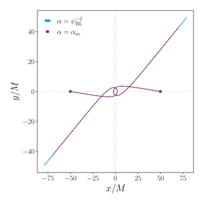
Figure 10: Trajectories of each BH using two different gauge choices for the initial lapse. The first choice is $\alpha=\psi^{-2}_{\rm BL}$, and the second the averaged lapse defined in Eq. (39). The dots denote the starting position of each BH.

Appendix B Mapping between scattering angle and potential coefficients

We here report the relations between the $w_{i}$ coefficients entering the radial potential $w_{n{\rm PM}}$, Eq. (IV.2), and the $\theta_{i}$ coefficients constituting the scattering angle $\theta_{n{\rm PM}}$, Eq. (20).

We start by recalling the equations linking the various energy variables to the $\gamma$ factor of the system:

$$\hat{E}^{\rm eob}_{\rm eff} \equiv\frac{E^{\rm eob}_{\rm eff}}{\mu}=\gamma\,,$$

$$\hat{E} \equiv\,\,\,\frac{E}{M}\,\,\,=\sqrt{1+2\nu\left(\gamma-1\right)}\,.$$ (40)

The relations between the nonspinning coefficients are known, and read

$$\theta_{1}^{\rm orb} =\frac{w_{1}^{\rm orb}}{2p_{\infty}}\,,$$

$$\theta_{2}^{\rm orb} =\frac{\pi}{4}w_{2}^{\rm orb}\,,$$

$$\theta_{3}^{\rm orb} =\frac{1}{p_{\infty}^{3}}\left[p_{\infty}^{4}w_{3}^{\rm orb}+\frac{1}{2}p_{\infty}^{2}w_{2}^{\rm orb}w_{1}^{\rm orb}-\left(w_{1}^{\rm orb}\right)^{3}\right]\,,$$

$$\theta_{4}^{\rm orb} =\frac{3\pi}{8}\left[p_{\infty}^{2}w_{4}^{\rm orb}+w_{3}^{\rm orb}w_{1}^{\rm orb}+\frac{1}{2}\left(w_{2}^{\rm orb}\right)^{2}\right]\,.$$ (41)

In the following, we list the relations containing spin terms relevant to this paper: linear relations up to 4PM, quadratic-in-spin up to 3PM, cubic and quartic-in-spin at 1PM and 2PM. At linear order in spins we get

$$\theta_{1}^{\rm S}= \frac{p_{\infty}}{2}w_{1}^{\rm S}\,,$$

$$\theta_{2}^{\rm S}= \frac{\pi}{4}\left(p_{\infty}^{2}w_{2}^{\rm S}+w_{1}^{\rm orb}w_{1}^{\rm S}\right)\,,$$

$$\theta_{3}^{\rm S}= \frac{1}{p_{\infty}}\Bigg{[}p_{\infty}^{4}w_{3}^{\rm S}+\frac{3}{2}p_{\infty}^{2}\left(w_{2}^{\rm orb}w_{1}^{\rm S}+w_{1}^{\rm orb}w_{2}^{\rm S}\right)$$

$$+\frac{3}{8}\left(w_{1}^{\rm orb}\right)^{2}w_{1}^{\rm S}\Bigg{]}\,,$$

$$\theta_{4}^{\rm S}= \frac{3\pi}{8}\Bigg{[}p_{\infty}^{4}w_{4}^{\rm S}+2p_{\infty}^{2}\left(w_{2}^{\rm orb}w_{2}^{\rm S}+w_{3}^{\rm orb}w_{1}^{\rm S}+w_{1}^{\rm orb}w_{3}^{\rm S}\right)$$

$$+\left(w_{1}^{\rm orb}\right)^{2}w_{2}^{\rm S}+2w_{2}^{\rm orb}w_{1}^{\rm orb}w_{1}^{\rm S}\Bigg{]}\,,$$ (42)

while the quadratic-in-spin terms read

$$\theta_{1}^{\rm S^{2}}= p_{\infty}w_{1}^{\rm S^{2}}\,,$$

$$\theta_{2}^{\rm S^{2}}= \frac{3\pi}{32}\left[3p_{\infty}^{2}\left(w_{1}^{\rm S}\right)^{2}+4p_{\infty}^{2}w_{2}^{\rm S^{2}}+4w_{1}^{\rm orb}w_{1}^{\rm S^{2}}\right]\,,$$

$$\theta_{3}^{\rm S^{2}}= \frac{1}{p_{\infty}}\Bigg{\{}\frac{4}{3}p_{\infty}^{4}\left(w_{3}^{\rm S^{2}}+2w_{2}^{\rm S}w_{1}^{\rm S}\right)+\frac{1}{2}\left(w_{1}^{\rm orb}\right)^{2}w_{1}^{\rm S^{2}}$$

$$+2p_{\infty}^{2}\left[w_{2}^{\rm orb}w_{1}^{\rm S^{2}}+w_{1}^{\rm orb}\left(w_{1}^{\rm S}\right)^{2}+w_{1}^{\rm orb}w_{2}^{\rm S^{2}}\right]\Bigg{\}}\,.$$ (43)

The cubic-in-spin and quadratic-in-spin contributions at 1PM order are simply

$$\theta_{1}^{\rm S^{3}}= p_{\infty}^{3}w_{1}^{\rm S^{3}}\,,$$

$$\theta_{1}^{\rm S^{4}}= \frac{4}{3}p_{\infty}^{3}w_{1}^{\rm S^{4}}\,,$$ (44)

while the 2PM coefficients can be obtained by

$$\theta_{2}^{\rm S^{3}}= \frac{3\pi}{8}p_{\infty}^{2}\left(p_{\infty}^{2}w_{2}^{\rm S^{3}}+2w_{1}^{\rm orb}w_{1}^{\rm S^{3}}+2w_{1}^{\rm S}w_{1}^{\rm S^{2}}\right)\,,$$

$$\theta_{2}^{\rm S^{4}}= \frac{15\pi}{64}p_{\infty}^{2}\Bigg{[}2p_{\infty}^{2}w_{2}^{\rm S^{4}}+5p_{\infty}^{2}w_{1}^{\rm S}w_{1}^{\rm S^{3}}$$

$$+4w_{1}^{\rm orb}w_{1}^{\rm S^{4}}+2\left(w_{1}^{\rm S_{2}}\right)^{2}\Bigg{]}\,.$$ (45)

The explicit values of the $w_{i}$ coefficients are given in the ancillary file of this paper.

Appendix C Additional Post-Minkowskian data points

In this appendix, we complement the PM results presented in the main paper.

In Figs. 11 and 12, we mimic Figs. 4 and 5 for the nonspinning systems with lower energy, $\hat{E}_{\rm in,1}\simeq 1.02264$. These figures confirm the outstanding agreement between EOB-PM predictions and NR results found in Ref. Damour et al. (2014b).

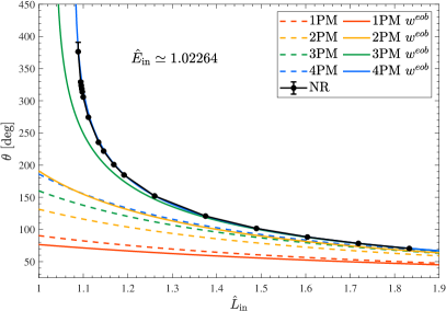
Figure 11: Scattering angles against initial angular momentum (as in Fig. 4) for the lower-energy simulations of equal-mass nonspinning BBHs.

Figure 12: Gravitational potential $V$ as a function of (center-of-mass, isotropic coordinates) separation (as in Fig. 5) for the lower energy simulations of equal-mass nonspinning BBHs.

In Tables 4 and Tables 5, we list the scattering angles for the presented NR simulations together with the corresponding best-performing analytical predictions (not considering 4PM spin-orbit terms), $\theta^{w}_{\rm 3PM}$ and $\theta^{w}_{\rm 4PM}$.

Table 4: NR equal-mass, nonspinning simulations presented in Table 1. The last two columns list the $w^{eob}$-resummed scattering angles at 3PM and 4PM as in Figs. 4 and 11. The scattering angles are replaced by dots when the black holes (are predicted to) plunge. An asterisk denotes uncertainty about an eventual plunge.

$\hat{E}_{\rm in}^{\rm{ADM}}$	$\hat{L}_{\rm in}^{\rm{ADM}}$	$\theta_{\rm{NR}}\left[\rm deg\right]$	$\theta^{w}_{\rm 3PM}\left[\rm deg\right]$	$\theta^{w}_{\rm 4PM}\left[\rm deg\right]$
1.02264	1.0769	$\cdots$	288.979	$\cdots$
1.02264	1.0884	$\phantom{\ast}376.275^{+0.026}_{-14.69}\ast$	266.491	379.310
1.02264	1.0941	$329.057^{+0.003}_{-1.534}$	257.257	341.135
1.02264	1.0952	$323.422^{+0.000}_{-1.914}$	255.589	335.476
1.02264	1.0964	$318.394^{+0.000}_{-1.575}$	253.808	329.728
1.02264	1.0975	$313.764^{+0.000}_{-1.331}$	252.209	324.803
1.02264	1.0998	$305.734^{+0.056}_{-0.694}$	248.965	315.401
1.02264	1.1113	$274.368^{+0.074}_{-0.016}$	234.475	280.337
1.02264	1.1342	$235.447^{+0.912}_{-0.003}$	211.830	238.507
1.02264	1.1456	$221.823^{+0.762}_{-0.002}$	202.691	224.179
1.02264	1.1686	$200.810^{+0.620}_{-0.004}$	187.190	201.991
1.02264	1.1915	$184.684^{+0.221}_{-0.002}$	174.595	185.411
1.02264	1.2602	$152.106^{+0.055}_{-0.446}$	147.085	152.231
1.02264	1.3748	$120.804^{+0.013}_{-0.307}$	118.731	120.821
1.02264	1.4893	$101.616^{+0.059}_{-0.002}$	100.654	101.704
1.02264	1.6039	$88.260^{+0.337}_{-0.002}$	87.828	88.423
1.02264	1.7185	$78.296^{+0.520}_{-0.002}$	78.150	78.515
1.02264	1.833	$70.404^{+0.927}_{-0.003}$	70.539	70.777
1.04032	1.1505	$\cdots$	295.902	$\cdots$
1.04032	1.1595	$\phantom{\ast}392.815^{+0.006}_{-7.477}\ast$	274.866	$\cdots$
1.04032	1.1655	$338.973^{+0.156}_{-0.756}$	263.305	430.914
1.04032	1.17	$317.637^{+0.142}_{-0.444}$	255.591	374.716
1.04032	1.1805	$283.359^{+0.343}_{-0.007}$	240.035	312.437
1.04032	1.1895	$262.825^{+0.749}_{-0.008}$	228.777	282.302
1.04032	1.2	$244.210^{+1.220}_{-0.005}$	217.439	257.740
1.04033	1.26	$184.138^{+0.439}_{-0.004}$	173.732	187.734
1.04033	1.32	$153.119^{+0.226}_{-0.227}$	147.539	154.603
1.04033	1.35	$141.986^{+0.244}_{-0.213}$	137.744	143.094
1.04033	1.41	$124.805^{+0.154}_{-0.238}$	122.169	125.487
1.04033	1.425	$121.233^{+0.180}_{-0.153}$	118.900	121.880
1.04033	1.44	$117.897^{+0.157}_{-0.091}$	115.828	118.517
1.04033	1.5	$106.459^{+0.207}_{-0.004}$	105.174	107.016
1.04033	1.8	$73.095^{+1.358}_{-0.006}$	73.374	73.826
1.04033	2.1	$56.489^{+1.242}_{-0.006}$	56.993	57.160
1.04033	2.4	$45.982^{+1.530}_{-0.008}$	46.791	46.868
1.05548	1.05	$\cdots$	$\cdots$	$\cdots$
1.05548	1.225	$354.118^{+0.307}_{-0.633}$	274.582	391.281
1.05548	1.26	$248.950^{+1.203}_{-0.005}$	222.675	280.445
1.05548	1.295	$206.064^{+1.479}_{-0.006}$	192.055	218.732
1.05548	1.33	$179.815^{+0.484}_{-0.006}$	170.787	186.552
1.05548	1.4	$146.516^{+0.354}_{-0.096}$	142.049	149.418
1.05548	1.575	$104.166^{+0.361}_{-0.006}$	103.162	105.287
1.05548	1.75	$82.275^{+0.924}_{-0.007}$	82.292	83.191
1.05548	1.925	$68.351^{+1.485}_{-0.007}$	68.882	69.339

Table 5: NR equal-mass, spinning simulations listed in Table 2. All systems were computed with fixed initial ADM energy $\hat{E}_{\rm in}^{\rm{ADM}}\simeq 1.02264$ and orbital ADM angular momentum $\hat{L}_{\rm in}^{\rm{ADM}}\simeq 1.14560$. The last two columns list the $w^{eob}$-resummed scattering angles at 3PM and 4PM as in Fig. 6.

$\chi_{1}$	$\chi_{2}$	$\theta_{\rm{NR}}\left[\rm deg\right]$	$\theta^{w}_{\rm 3PM}\left[\rm deg\right]$	$\theta^{w}_{\rm 4PM}\left[\rm deg\right]$
-0.3	-0.3	$\cdots$	209.786	494.626
-0.25	-0.25	$\phantom{\ast}367.545^{+0.000}_{-4.840}\ast$	266.889	351.203
-0.23	-0.23	$334.345^{+0.084}_{-1.573}$	266.305	327.892
-0.22	-0.22	$322.693^{+0.099}_{-1.004}$	258.352	318.528
-0.21	-0.21	$312.795^{+0.187}_{-0.364}$	251.257	310.189
-0.2	-0.2	$303.884^{+0.222}_{-0.466}$	247.895	302.522
-0.17	-0.17	$286.603^{+0.154}_{-0.010}$	238.849	283.736
-0.16	-0.16	$277.849^{+0.230}_{-0.003}$	236.080	278.413
-0.15	-0.15	$272.603^{+0.260}_{-0.003}$	233.369	273.354
-0.1	-0.1	$251.028^{+0.559}_{-0.003}$	221.462	252.778
-0.05	-0.05	$234.568^{+0.845}_{-0.003}$	211.364	236.915
-0.00	-0.00	$221.823^{+0.762}_{-0.002}$	202.691	224.179
-0.05	-0.05	$211.195^{+0.610}_{-0.002}$	195.096	213.564
-0.05	-0.05	$221.866^{+0.643}_{-0.002}$	202.986	224.175
-0.10	-0.10	$202.608^{+0.388}_{-0.002}$	188.382	204.533
-0.15	-0.15	$194.542^{+0.183}_{-0.001}$	182.347	196.652
-0.15	-0.15	$221.887^{+0.637}_{-0.002}$	202.691	224.186
-0.20	-0.2	$221.819^{+0.863}_{-0.003}$	202.698	224.201
-0.20	-0.20	$187.838^{+0.020}_{-0.141}$	176.910	189.726
-0.30	-0.30	$176.586^{+0.001}_{-0.653}$	167434	177.997
-0.40	-0.4	$221.847^{+0.849}_{-0.003}$	202.771	224.357
-0.40	-0.00	$188.138^{+0.008}_{-0.132}$	1776.927	189.759
-0.40	-0.40	$167.545^{+0.002}_{-0.947}$	159.411	168.358
-0.50	-0.3	$203.121^{+0.477}_{-0.002}$	188.440	204.657
-0.60	-0.6	$222.080^{+0.808}_{-0.003}$	202.912	224.646
-0.60	-0.00	$177.629^{+0.001}_{-0.645}$	167.462	178.053
-0.60	-0.60	$154.139^{+0.005}_{-1.443}$	146.410	153.206
-0.70	-0.3	$190.407^{+0.013}_{-0.164}$	177.005	189.915
-0.70	-0.30	$160.935^{+0.004}_{-1.274}$	152.489	160.234
-0.80	-0.8	$221.679^{+0.489}_{-0.002}$	203.145	225.114
-0.80	-0.5	$198.993^{+0.237}_{-0.001}$	182.518	196.996
-0.80	-0.00	$170.394^{+0.003}_{-1.026}$	159.445	168.433
-0.80	-0.20	$162.069^{+0.005}_{-1.308}$	152.494	160.249
-0.80	-0.50	$152.303^{+0.006}_{-1.640}$	143.642	150.049
-0.80	-0.80	$145.357^{+0.006}_{-1.528}$	136.199	141.643

Finally, we compare the spin dependence of the NR scattering angles to PM predictions in the small spin range. Using the simplifying fact that we are considering equal-mass systems, and the relative scattering angle $\theta_{\rm rel}=\frac{1}{2}(\theta_{1}+\theta_{2})$, we can write, at quadratic order in spins, the simple general template

$$\theta_{\rm rel}\left(\gamma,j;\chi_{i}\right) \overset{(m_{1}=m_{2})}{=}~{}\theta_{0}\left(\gamma,j\right)+\,\theta_{\chi_{+}}\left(\gamma,j\right)\chi_{+}$$

$$+\theta_{\chi_{+}^{2}}\left(\gamma,j\right)\chi_{+}^{2}+\theta_{\chi_{-}^{2}}\left(\gamma,j\right)\chi_{-}^{2}+\mathcal{O}\left[\chi^{3}\right].$$ (46)

We can, in principle, determine the $\theta_{i}$ coefficients for the initial energy and angular momentum of our simulations, $(\hat{E}_{\rm in},\hat{L}_{\rm in})\simeq(1.02264,1.1456)$ by fitting the scattering angles for configurations with small (absolute) values of the spins. We decided to focus on the 6 configurations with $|\chi_{1/2}|\leq 0.1$ and to fit them to the template Eq. (C) (truncated to quadratic terms). We so obtained the following values:

$$\theta_{0}^{\rm fit} =3.872\pm 0.048,$$

$$\theta_{\chi_{+}}^{\rm fit} =-4.211\pm 0.031,$$

$$\theta_{\chi_{+}^{2}}^{\rm fit} =8.75\pm 0.60,$$

$$\theta_{\chi_{-}^{2}}^{\rm fit} =0.6\pm 3.1.$$ (47)

The reduced chi-squared of this fit is $\chi^{2}/(6-4)\simeq 1.17$ (corresponding to six data points and four degrees of freedom). This value is probably affected by the fact that we are assuming constant initial data, while the energy slightly changes between simulations. Let us emphasize that we could not extract a meaningful value for the $\theta_{\chi_{-}^{2}}^{\rm fit}$ coefficient, consistently with our finding that these effects are subdominant (even for higher spin values).

In Table 6 we compare these NR-fitting coefficients to their (PM-expanded and $w^{eob}$-resummed) analytical analogs. In order to extract $w^{eob}_{\rm 3PM}$ and $w^{eob}_{\rm 4PM}$ (not including 4PM spin-orbit terms), we repeat the same fitting procedure employed for the NR angles (but setting the initial energy to the constant, average, value). For the considered initial data, $(\hat{E}_{\rm in},\hat{L}_{\rm in})\simeq(1.02264,1.1456)$, the PM-expanded predictions are not satisfactory, as could be deduced from Fig. 6. The successive PM orders show a slow convergence towards the numerical results. The EOB-resummed equivalents, instead, are in good agreement with the numerical estimates, with the $w^{eob}_{\rm 4PM}$ values mostly agreeing within one standard deviation with the NR ones.

Table 6: Small-spin dependence of the scattering angle for $\hat{E}_{\rm in}\simeq 1.02264$ and $\hat{L}_{\rm in}\simeq 1.1456$. PM predictions for the different spin-orders (if available) together with values extracted by fitting NR data [Eq. (C)].

	3PM	4PM	$w^{eob}_{\rm 3PM}$	$w^{eob}_{\rm 4PM}$	NR
$\theta_{0}$	2.255	2.519	3.543	3.920	$3.872\pm 0.048$
$\theta_{\chi_{+}}$	-0.433	-0.621	-2.895	-4.221	$-4.211\pm 0.031$
$\theta_{\chi_{+}^{2}}$	0.085	$\cdots$	3.898	7.904	$8.75\pm 0.60$
$\theta_{\chi_{-}^{2}}$	-0.001	$\cdots$	0.034	0.198	$0.6\pm 3.1$

References

- Abbott et al. (2019) B. P. Abbott et al. (LIGO Scientific, Virgo), “GWTC-1: A Gravitational-Wave Transient Catalog of Compact Binary Mergers Observed by LIGO and Virgo during the First and Second Observing Runs,” Phys. Rev. X9, 031040 (2019), arXiv:1811.12907 [astro-ph.HE] .
- Abbott et al. (2021a) R. Abbott et al. (LIGO Scientific, Virgo), “GWTC-2: Compact Binary Coalescences Observed by LIGO and Virgo During the First Half of the Third Observing Run,” Phys. Rev. X 11, 021053 (2021a), arXiv:2010.14527 [gr-qc] .
- Abbott et al. (2021b) R. Abbott et al. (LIGO Scientific, VIRGO, KAGRA), “GWTC-3: Compact Binary Coalescences Observed by LIGO and Virgo During the Second Part of the Third Observing Run,” (2021b), arXiv:2111.03606 [gr-qc] .
- Nitz et al. (2023) Alexander H. Nitz, Sumit Kumar, Yi-Fan Wang, Shilpa Kastha, Shichao Wu, Marlin Schäfer, Rahul Dhurkunde, and Collin D. Capano, “4-OGC: Catalog of Gravitational Waves from Compact Binary Mergers,” Astrophys. J. 946, 59 (2023), arXiv:2112.06878 [astro-ph.HE] .
- Olsen et al. (2022) Seth Olsen, Tejaswi Venumadhav, Jonathan Mushkin, Javier Roulet, Barak Zackay, and Matias Zaldarriaga, “New binary black hole mergers in the LIGO-Virgo O3a data,” Phys. Rev. D 106, 043009 (2022), arXiv:2201.02252 [astro-ph.HE] .
- Pretorius (2005) Frans Pretorius, “Evolution of binary black hole spacetimes,” Phys. Rev. Lett. 95, 121101 (2005), arXiv:gr-qc/0507014 .
- Campanelli et al. (2006a) Manuela Campanelli, C. O. Lousto, P. Marronetti, and Y. Zlochower, “Accurate Evolutions of Orbiting Black-Hole Binaries Without Excision,” Phys. Rev. Lett. 96, 111101 (2006a), arXiv:gr-qc/0511048 .
- Mroue et al. (2013) Abdul H. Mroue, Mark A. Scheel, Bela Szilagyi, Harald P. Pfeiffer, Michael Boyle, et al., “A catalog of 174 binary black-hole simulations for gravitational-wave astronomy,” Phys.Rev.Lett. 111, 241104 (2013), arXiv:1304.6077 [gr-qc] .
- Husa et al. (2016) Sascha Husa, Sebastian Khan, Mark Hannam, Michael Pürrer, Frank Ohme, Xisco Jiménez Forteza, and Alejandro Bohé, “Frequency-domain gravitational waves from nonprecessing black-hole binaries. I. New numerical waveforms and anatomy of the signal,” Phys. Rev. D93, 044006 (2016), arXiv:1508.07250 [gr-qc] .
- Jani et al. (2016) Karan Jani, James Healy, James A. Clark, Lionel London, Pablo Laguna, and Deirdre Shoemaker, “Georgia Tech Catalog of Gravitational Waveforms,” Class. Quant. Grav. 33, 204001 (2016), arXiv:1605.03204 [gr-qc] .
- Boyle et al. (2019) Michael Boyle et al., “The SXS Collaboration catalog of binary black hole simulations,” Class. Quant. Grav. 36, 195006 (2019), arXiv:1904.04831 [gr-qc] .
- Healy et al. (2019) James Healy, Carlos O. Lousto, Jacob Lange, Richard O’Shaughnessy, Yosef Zlochower, and Manuela Campanelli, “Second RIT binary black hole simulations catalog and its application to gravitational waves parameter estimation,” Phys. Rev. D 100, 024021 (2019), arXiv:1901.02553 [gr-qc] .
- Hamilton et al. (2023) Eleanor Hamilton et al., “A catalogue of precessing black-hole-binary numerical-relativity simulations,” (2023), arXiv:2303.05419 [gr-qc] .
- Field et al. (2014) Scott E. Field, Chad R. Galley, Jan S. Hesthaven, Jason Kaye, and Manuel Tiglio, “Fast prediction and evaluation of gravitational waveforms using surrogate models,” Phys.Rev. X4, 031006 (2014), arXiv:1308.3565 [gr-qc] .
- Blackman et al. (2017) Jonathan Blackman, Scott E. Field, Mark A. Scheel, Chad R. Galley, Daniel A. Hemberger, Patricia Schmidt, and Rory Smith, “A Surrogate Model of Gravitational Waveforms from Numerical Relativity Simulations of Precessing Binary Black Hole Mergers,” Phys. Rev. D95, 104023 (2017), arXiv:1701.00550 [gr-qc] .
- Varma et al. (2019) Vijay Varma, Scott E. Field, Mark A. Scheel, Jonathan Blackman, Davide Gerosa, Leo C. Stein, Lawrence E. Kidder, and Harald P. Pfeiffer, “Surrogate models for precessing binary black hole simulations with unequal masses,” Phys. Rev. Research. 1, 033015 (2019), arXiv:1905.09300 [gr-qc] .
- Buonanno and Damour (1999) A. Buonanno and T. Damour, “Effective one-body approach to general relativistic two-body dynamics,” Phys. Rev. D59, 084006 (1999), arXiv:gr-qc/9811091 .
- Buonanno and Damour (2000) Alessandra Buonanno and Thibault Damour, “Transition from inspiral to plunge in binary black hole coalescences,” Phys. Rev. D62, 064015 (2000), arXiv:gr-qc/0001013 .
- Gamba et al. (2022a) Rossella Gamba, Sarp Akçay, Sebastiano Bernuzzi, and Jake Williams, “Effective-one-body waveforms for precessing coalescing compact binaries with post-Newtonian twist,” Phys. Rev. D 106, 024020 (2022a), arXiv:2111.03675 [gr-qc] .
- Ossokine et al. (2020) Serguei Ossokine et al., “Multipolar Effective-One-Body Waveforms for Precessing Binary Black Holes: Construction and Validation,” Phys. Rev. D 102, 044055 (2020), arXiv:2004.09442 [gr-qc] .
- Ramos-Buades et al. (2023) Antoni Ramos-Buades, Alessandra Buonanno, Héctor Estellés, Mohammed Khalil, Deyan P. Mihaylov, Serguei Ossokine, Lorenzo Pompili, and Mahlet Shiferaw, “SEOBNRv5PHM: Next generation of accurate and efficient multipolar precessing-spin effective-one-body waveforms for binary black holes,” (2023), arXiv:2303.18046 [gr-qc] .
- Hannam et al. (2014) Mark Hannam, Patricia Schmidt, Alejandro Bohé, Leïla Haegel, Sascha Husa, Frank Ohme, Geraint Pratten, and Michael Pürrer, “Simple Model of Complete Precessing Black-Hole-Binary Gravitational Waveforms,” Phys. Rev. Lett. 113, 151101 (2014), arXiv:1308.3271 [gr-qc] .
- Pratten et al. (2020) Geraint Pratten, Sascha Husa, Cecilio Garcia-Quiros, Marta Colleoni, Antoni Ramos-Buades, Hector Estelles, and Rafel Jaume, “Setting the cornerstone for a family of models for gravitational waves from compact binaries: The dominant harmonic for nonprecessing quasicircular black holes,” Phys. Rev. D 102, 064001 (2020), arXiv:2001.11412 [gr-qc] .
- García-Quirós et al. (2020) Cecilio García-Quirós, Marta Colleoni, Sascha Husa, Héctor Estellés, Geraint Pratten, Antoni Ramos-Buades, Maite Mateu-Lucena, and Rafel Jaume, “Multimode frequency-domain model for the gravitational wave signal from nonprecessing black-hole binaries,” Phys. Rev. D 102, 064002 (2020), arXiv:2001.10914 [gr-qc] .
- Pratten et al. (2021) Geraint Pratten et al., “Computationally efficient models for the dominant and subdominant harmonic modes of precessing binary black holes,” Phys. Rev. D 103, 104056 (2021), arXiv:2004.06503 [gr-qc] .
- Hamilton et al. (2021) Eleanor Hamilton, Lionel London, Jonathan E. Thompson, Edward Fauchon-Jones, Mark Hannam, Chinmay Kalaghatgi, Sebastian Khan, Francesco Pannarale, and Alex Vano-Vinuales, “Model of gravitational waves from precessing black-hole binaries through merger and ringdown,” Phys. Rev. D 104, 124027 (2021), arXiv:2107.08876 [gr-qc] .
- Blanchet and Damour (1989) L. Blanchet and T. Damour, “Postnewtonian Generation of Gravitational Waves,” Ann. Inst. H. Poincaré Phys. Theor. 50, 377–408 (1989).
- Blanchet (2014) Luc Blanchet, “Gravitational Radiation from Post-Newtonian Sources and Inspiralling Compact Binaries,” Living Rev. Relativity 17, 2 (2014), arXiv:1310.1528 [gr-qc] .
- Damour et al. (2014a) Thibault Damour, Piotr Jaranowski, and Gerhard Schäfer, “Nonlocal-in-time action for the fourth post-Newtonian conservative dynamics of two-body systems,” Phys. Rev. D 89, 064058 (2014a), arXiv:1401.4548 [gr-qc] .
- Levi and Steinhoff (2016) Michele Levi and Jan Steinhoff, “Next-to-next-to-leading order gravitational spin-orbit coupling via the effective field theory for spinning objects in the post-Newtonian scheme,” JCAP 1601, 011 (2016), arXiv:1506.05056 [gr-qc] .
- Bini and Damour (2017a) Donato Bini and Thibault Damour, “Gravitational scattering of two black holes at the fourth post-Newtonian approximation,” Phys. Rev. D96, 064021 (2017a), arXiv:1706.06877 [gr-qc] .
- Schaefer and Jaranowski (2018) Gerhard Schaefer and Piotr Jaranowski, “Hamiltonian formulation of general relativity and post-Newtonian dynamics of compact binaries,” Living Rev. Rel. 21, 7 (2018), arXiv:1805.07240 [gr-qc] .
- Bini et al. (2019) Donato Bini, Thibault Damour, and Andrea Geralico, “Novel approach to binary dynamics: application to the fifth post-Newtonian level,” Phys. Rev. Lett. 123, 231104 (2019), arXiv:1909.02375 [gr-qc] .
- Bini et al. (2020a) Donato Bini, Thibault Damour, and Andrea Geralico, “Binary dynamics at the fifth and fifth-and-a-half post-Newtonian orders,” Phys. Rev. D 102, 024062 (2020a), arXiv:2003.11891 [gr-qc] .
- Bini et al. (2020b) Donato Bini, Thibault Damour, and Andrea Geralico, “Sixth post-Newtonian local-in-time dynamics of binary systems,” Phys. Rev. D 102, 024061 (2020b), arXiv:2004.05407 [gr-qc] .
- Bini et al. (2020c) Donato Bini, Thibault Damour, and Andrea Geralico, “Sixth post-Newtonian nonlocal-in-time dynamics of binary systems,” Phys. Rev. D 102, 084047 (2020c), arXiv:2007.11239 [gr-qc] .
- Antonelli et al. (2020) Andrea Antonelli, Chris Kavanagh, Mohammed Khalil, Jan Steinhoff, and Justin Vines, “Gravitational spin-orbit and aligned spin1-spin2 couplings through third-subleading post-Newtonian orders,” Phys. Rev. D 102, 124024 (2020), arXiv:2010.02018 [gr-qc] .
- Blümlein et al. (2021) J. Blümlein, A. Maier, P. Marquard, and G. Schäfer, “The fifth-order post-Newtonian Hamiltonian dynamics of two-body systems from an effective field theory approach: potential contributions,” Nucl. Phys. B 965, 115352 (2021), arXiv:2010.13672 [gr-qc] .
- Blümlein et al. (2022) J. Blümlein, A. Maier, P. Marquard, and G. Schäfer, “The fifth-order post-Newtonian Hamiltonian dynamics of two-body systems from an effective field theory approach,” Nucl. Phys. B 983, 115900 (2022), arXiv:2110.13822 [gr-qc] .
- Mandal et al. (2023a) Manoj K. Mandal, Pierpaolo Mastrolia, Raj Patil, and Jan Steinhoff, “Gravitational spin-orbit Hamiltonian at NNNLO in the post-Newtonian framework,” JHEP 03, 130 (2023a), arXiv:2209.00611 [hep-th] .
- Mandal et al. (2023b) Manoj K. Mandal, Pierpaolo Mastrolia, Raj Patil, and Jan Steinhoff, “Gravitational quadratic-in-spin Hamiltonian at NNNLO in the post-Newtonian framework,” JHEP 07, 128 (2023b), arXiv:2210.09176 [hep-th] .
- Reitze et al. (2019) David Reitze et al., “Cosmic Explorer: The U.S. Contribution to Gravitational-Wave Astronomy beyond LIGO,” Bull. Am. Astron. Soc. 51, 035 (2019), arXiv:1907.04833 [astro-ph.IM] .
- Punturo et al. (2010) M. Punturo, M. Abernathy, F. Acernese, B. Allen, N. Andersson, et al., “The Einstein Telescope: A third-generation gravitational wave observatory,” Class.Quant.Grav. 27, 194002 (2010).
- Amaro-Seoane et al. (2017) Pau Amaro-Seoane et al. (LISA), “Laser Interferometer Space Antenna,” (2017), arXiv:1702.00786 [astro-ph.IM] .
- Romero-Shaw et al. (2020) Isobel M. Romero-Shaw, Paul D. Lasky, Eric Thrane, and Juan Calderon Bustillo, “GW190521: orbital eccentricity and signatures of dynamical formation in a binary black hole merger signal,” Astrophys. J. Lett. 903, L5 (2020), arXiv:2009.04771 [astro-ph.HE] .
- Bustillo et al. (2021) Juan Calderón Bustillo, Nicolas Sanchis-Gual, Alejandro Torres-Forné, and José A. Font, “Confusing Head-On Collisions with Precessing Intermediate-Mass Binary Black Hole Mergers,” Phys. Rev. Lett. 126, 201101 (2021), arXiv:2009.01066 [gr-qc] .
- Gayathri et al. (2022) V. Gayathri, J. Healy, J. Lange, B. O’Brien, M. Szczepanczyk, Imre Bartos, M. Campanelli, S. Klimenko, C. O. Lousto, and R. O’Shaughnessy, “Eccentricity estimate for black hole mergers with numerical relativity simulations,” Nature Astron. 6, 344–349 (2022), arXiv:2009.05461 [astro-ph.HE] .
- Gamba et al. (2022b) Rossella Gamba, Matteo Breschi, Gregorio Carullo, Piero Rettegno, Simone Albanesi, Sebastiano Bernuzzi, and Alessandro Nagar, “GW190521 as a dynamical capture of two nonspinning black holes,” Nat. Astron. (2022b), 10.1038/s41550-022-01813-w, arXiv:2106.05575 [gr-qc] .
- O’Leary et al. (2006) Ryan M. O’Leary, Frederic A. Rasio, John M. Fregeau, Natalia Ivanova, and Richard W. O’Shaughnessy, “Binary mergers and growth of black holes in dense star clusters,” Astrophys. J. 637, 937–951 (2006), arXiv:astro-ph/0508224 .
- O’Leary et al. (2009) Ryan M. O’Leary, Bence Kocsis, and Abraham Loeb, “Gravitational waves from scattering of stellar-mass black holes in galactic nuclei,” Mon. Not. Roy. Astron. Soc. 395, 2127–2146 (2009), arXiv:0807.2638 [astro-ph] .
- Samsing et al. (2014) Johan Samsing, Morgan MacLeod, and Enrico Ramirez-Ruiz, “The Formation of Eccentric Compact Binary Inspirals and the Role of Gravitational Wave Emission in Binary-Single Stellar Encounters,” Astrophys. J. 784, 71 (2014), arXiv:1308.2964 [astro-ph.HE] .
- Rodriguez et al. (2016) Carl L. Rodriguez, Sourav Chatterjee, and Frederic A. Rasio, “Binary Black Hole Mergers from Globular Clusters: Masses, Merger Rates, and the Impact of Stellar Evolution,” Phys. Rev. D93, 084029 (2016), arXiv:1602.02444 [astro-ph.HE] .
- Belczynski et al. (2016) Krzysztof Belczynski, Daniel E. Holz, Tomasz Bulik, and Richard O’Shaughnessy, “The first gravitational-wave source from the isolated evolution of two 40-100 Msun stars,” Nature 534, 512 (2016), arXiv:1602.04531 [astro-ph.HE] .
- Samsing (2018) Johan Samsing, “Eccentric Black Hole Mergers Forming in Globular Clusters,” Phys. Rev. D97, 103014 (2018), arXiv:1711.07452 [astro-ph.HE] .
- Romero-Shaw et al. (2019) Isobel M. Romero-Shaw, Paul D. Lasky, and Eric Thrane, “Searching for Eccentricity: Signatures of Dynamical Formation in the First Gravitational-Wave Transient Catalogue of LIGO and Virgo,” Mon. Not. Roy. Astron. Soc. 490, 5210–5216 (2019), arXiv:1909.05466 [astro-ph.HE] .
- Zevin et al. (2021) Michael Zevin, Isobel M. Romero-Shaw, Kyle Kremer, Eric Thrane, and Paul D. Lasky, “Implications of Eccentric Observations on Binary Black Hole Formation Channels,” Astrophys. J. Lett. 921, L43 (2021), arXiv:2106.09042 [astro-ph.HE] .
- Damour (2016) Thibault Damour, “Gravitational scattering, post-Minkowskian approximation and Effective One-Body theory,” Phys. Rev. D94, 104015 (2016), arXiv:1609.00354 [gr-qc] .
- Damour (2018) Thibault Damour, “High-energy gravitational scattering and the general relativistic two-body problem,” Phys. Rev. D97, 044038 (2018), arXiv:1710.10599 [gr-qc] .
- Cheung et al. (2018) Clifford Cheung, Ira Z. Rothstein, and Mikhail P. Solon, “From Scattering Amplitudes to Classical Potentials in the Post-Minkowskian Expansion,” Phys. Rev. Lett. 121, 251101 (2018), arXiv:1808.02489 [hep-th] .
- Guevara et al. (2019a) Alfredo Guevara, Alexander Ochirov, and Justin Vines, “Scattering of Spinning Black Holes from Exponentiated Soft Factors,” JHEP 09, 056 (2019a), arXiv:1812.06895 [hep-th] .
- Kosower et al. (2019) David A. Kosower, Ben Maybee, and Donal O’Connell, “Amplitudes, Observables, and Classical Scattering,” JHEP 02, 137 (2019), arXiv:1811.10950 [hep-th] .
- Bern et al. (2019a) Zvi Bern, Clifford Cheung, Radu Roiban, Chia-Hsien Shen, Mikhail P. Solon, and Mao Zeng, “Scattering Amplitudes and the Conservative Hamiltonian for Binary Systems at Third Post-Minkowskian Order,” Phys. Rev. Lett. 122, 201603 (2019a), arXiv:1901.04424 [hep-th] .
- Bern et al. (2019b) Zvi Bern, Clifford Cheung, Radu Roiban, Chia-Hsien Shen, Mikhail P. Solon, and Mao Zeng, “Black Hole Binary Dynamics from the Double Copy and Effective Theory,” JHEP 10, 206 (2019b), arXiv:1908.01493 [hep-th] .
- Bjerrum-Bohr et al. (2020) N. E. J. Bjerrum-Bohr, Andrea Cristofoli, and Poul H. Damgaard, “Post-Minkowskian Scattering Angle in Einstein Gravity,” JHEP 08, 038 (2020), arXiv:1910.09366 [hep-th] .
- Herrmann et al. (2021) Enrico Herrmann, Julio Parra-Martinez, Michael S. Ruf, and Mao Zeng, “Radiative classical gravitational observables at (G3) from scattering amplitudes,” JHEP 10, 148 (2021), arXiv:2104.03957 [hep-th] .
- Bern et al. (2021a) Zvi Bern, Julio Parra-Martinez, Radu Roiban, Michael S. Ruf, Chia-Hsien Shen, Mikhail P. Solon, and Mao Zeng, “Scattering Amplitudes and Conservative Binary Dynamics at ,” Phys. Rev. Lett. 126, 171601 (2021a), arXiv:2101.07254 [hep-th] .
- Bern et al. (2022) Zvi Bern, Julio Parra-Martinez, Radu Roiban, Michael S. Ruf, Chia-Hsien Shen, Mikhail P. Solon, and Mao Zeng, “Scattering Amplitudes, the Tail Effect, and Conservative Binary Dynamics at O(G4),” Phys. Rev. Lett. 128, 161103 (2022), arXiv:2112.10750 [hep-th] .
- Bjerrum-Bohr et al. (2021) N. Emil J. Bjerrum-Bohr, Poul H. Damgaard, Ludovic Planté, and Pierre Vanhove, “The amplitude for classical gravitational scattering at third Post-Minkowskian order,” JHEP 08, 172 (2021), arXiv:2105.05218 [hep-th] .
- Manohar et al. (2022) Aneesh V. Manohar, Alexander K. Ridgway, and Chia-Hsien Shen, “Radiated Angular Momentum and Dissipative Effects in Classical Scattering,” Phys. Rev. Lett. 129, 121601 (2022), arXiv:2203.04283 [hep-th] .
- Saketh et al. (2022) M. V. S. Saketh, Justin Vines, Jan Steinhoff, and Alessandra Buonanno, “Conservative and radiative dynamics in classical relativistic scattering and bound systems,” Phys. Rev. Res. 4, 013127 (2022), arXiv:2109.05994 [gr-qc] .
- Koemans Collado et al. (2019) Arnau Koemans Collado, Paolo Di Vecchia, and Rodolfo Russo, “Revisiting the second post-Minkowskian eikonal and the dynamics of binary black holes,” Phys. Rev. D 100, 066028 (2019), arXiv:1904.02667 [hep-th] .
- Di Vecchia et al. (2020) Paolo Di Vecchia, Stephen G. Naculich, Rodolfo Russo, Gabriele Veneziano, and Chris D. White, “A tale of two exponentiations in = 8 supergravity at subleading level,” JHEP 03, 173 (2020), arXiv:1911.11716 [hep-th] .
- Di Vecchia et al. (2021) Paolo Di Vecchia, Carlo Heissenberg, Rodolfo Russo, and Gabriele Veneziano, “The eikonal approach to gravitational scattering and radiation at (G3),” JHEP 07, 169 (2021), arXiv:2104.03256 [hep-th] .
- Di Vecchia et al. (2022) Paolo Di Vecchia, Carlo Heissenberg, Rodolfo Russo, and Gabriele Veneziano, “The eikonal operator at arbitrary velocities I: the soft-radiation limit,” JHEP 07, 039 (2022), arXiv:2204.02378 [hep-th] .
- Kälin and Porto (2020a) Gregor Kälin and Rafael A. Porto, “Post-Minkowskian Effective Field Theory for Conservative Binary Dynamics,” JHEP 11, 106 (2020a), arXiv:2006.01184 [hep-th] .
- Kälin et al. (2020) Gregor Kälin, Zhengwen Liu, and Rafael A. Porto, “Conservative Dynamics of Binary Systems to Third Post-Minkowskian Order from the Effective Field Theory Approach,” Phys. Rev. Lett. 125, 261103 (2020), arXiv:2007.04977 [hep-th] .
- Mougiakakos et al. (2021) Stavros Mougiakakos, Massimiliano Maria Riva, and Filippo Vernizzi, “Gravitational Bremsstrahlung in the post-Minkowskian effective field theory,” Phys. Rev. D 104, 024041 (2021), arXiv:2102.08339 [gr-qc] .
- Dlapa et al. (2022a) Christoph Dlapa, Gregor Kälin, Zhengwen Liu, and Rafael A. Porto, “Dynamics of binary systems to fourth Post-Minkowskian order from the effective field theory approach,” Phys. Lett. B 831, 137203 (2022a), arXiv:2106.08276 [hep-th] .
- Dlapa et al. (2022b) Christoph Dlapa, Gregor Kälin, Zhengwen Liu, and Rafael A. Porto, “Conservative Dynamics of Binary Systems at Fourth Post-Minkowskian Order in the Large-Eccentricity Expansion,” Phys. Rev. Lett. 128, 161104 (2022b), arXiv:2112.11296 [hep-th] .
- Kälin et al. (2023) Gregor Kälin, Jakob Neef, and Rafael A. Porto, “Radiation-reaction in the Effective Field Theory approach to Post-Minkowskian dynamics,” JHEP 01, 140 (2023), arXiv:2207.00580 [hep-th] .
- Dlapa et al. (2023) Christoph Dlapa, Gregor Kälin, Zhengwen Liu, Jakob Neef, and Rafael A. Porto, “Radiation Reaction and Gravitational Waves at Fourth Post-Minkowskian Order,” Phys. Rev. Lett. 130, 101401 (2023), arXiv:2210.05541 [hep-th] .
- Mogull et al. (2021) Gustav Mogull, Jan Plefka, and Jan Steinhoff, “Classical black hole scattering from a worldline quantum field theory,” JHEP 02, 048 (2021), arXiv:2010.02865 [hep-th] .
- Riva and Vernizzi (2021) Massimiliano Maria Riva and Filippo Vernizzi, “Radiated momentum in the post-Minkowskian worldline approach via reverse unitarity,” JHEP 11, 228 (2021), arXiv:2110.10140 [hep-th] .
- Jakobsen et al. (2021) Gustav Uhre Jakobsen, Gustav Mogull, Jan Plefka, and Jan Steinhoff, “Classical Gravitational Bremsstrahlung from a Worldline Quantum Field Theory,” Phys. Rev. Lett. 126, 201103 (2021), arXiv:2101.12688 [gr-qc] .
- Jakobsen et al. (2022) Gustav Uhre Jakobsen, Gustav Mogull, Jan Plefka, and Benjamin Sauer, “All things retarded: radiation-reaction in worldline quantum field theory,” JHEP 10, 128 (2022), arXiv:2207.00569 [hep-th] .
- Bini et al. (2021) Donato Bini, Thibault Damour, and Andrea Geralico, “Radiative contributions to gravitational scattering,” Phys. Rev. D 104, 084031 (2021), arXiv:2107.08896 [gr-qc] .
- Bini and Damour (2022) Donato Bini and Thibault Damour, “Radiation-reaction and angular momentum loss at the second post-Minkowskian order,” Phys. Rev. D 106, 124049 (2022), arXiv:2211.06340 [gr-qc] .
- Bini et al. (2023) Donato Bini, Thibault Damour, and Andrea Geralico, “Radiated momentum and radiation reaction in gravitational two-body scattering including time-asymmetric effects,” Phys. Rev. D 107, 024012 (2023), arXiv:2210.07165 [gr-qc] .
- Chiaramello and Nagar (2020) Danilo Chiaramello and Alessandro Nagar, “Faithful analytical effective-one-body waveform model for spin-aligned, moderately eccentric, coalescing black hole binaries,” Phys. Rev. D 101, 101501 (2020), arXiv:2001.11736 [gr-qc] .
- Nagar et al. (2021) Alessandro Nagar, Alice Bonino, and Piero Rettegno, “Effective one-body multipolar waveform model for spin-aligned, quasicircular, eccentric, hyperbolic black hole binaries,” Phys. Rev. D 103, 104021 (2021), arXiv:2101.08624 [gr-qc] .
- Placidi et al. (2022) Andrea Placidi, Simone Albanesi, Alessandro Nagar, Marta Orselli, Sebastiano Bernuzzi, and Gianluca Grignani, “Exploiting Newton-factorized, 2PN-accurate waveform multipoles in effective-one-body models for spin-aligned noncircularized binaries,” Phys. Rev. D 105, 104030 (2022), arXiv:2112.05448 [gr-qc] .
- Khalil et al. (2021) Mohammed Khalil, Alessandra Buonanno, Jan Steinhoff, and Justin Vines, “Radiation-reaction force and multipolar waveforms for eccentric, spin-aligned binaries in the effective-one-body formalism,” Phys. Rev. D 104, 024046 (2021), arXiv:2104.11705 [gr-qc] .
- Ramos-Buades et al. (2022a) Antoni Ramos-Buades, Alessandra Buonanno, Mohammed Khalil, and Serguei Ossokine, “Effective-one-body multipolar waveforms for eccentric binary black holes with nonprecessing spins,” Phys. Rev. D 105, 044035 (2022a), arXiv:2112.06952 [gr-qc] .
- Nagar and Rettegno (2021) Alessandro Nagar and Piero Rettegno, “Next generation: Impact of high-order analytical information on effective one body waveform models for noncircularized, spin-aligned black hole binaries,” Phys. Rev. D 104, 104004 (2021), arXiv:2108.02043 [gr-qc] .
- Khalil et al. (2022) Mohammed Khalil, Alessandra Buonanno, Jan Steinhoff, and Justin Vines, “Energetics and scattering of gravitational two-body systems at fourth post-Minkowskian order,” Phys. Rev. D 106, 024042 (2022), arXiv:2204.05047 [gr-qc] .
- Hinder et al. (2010) Ian Hinder, Frank Herrmann, Pablo Laguna, and Deirdre Shoemaker, “Comparisons of eccentric binary black hole simulations with post-Newtonian models,” Phys. Rev. D82, 024033 (2010), arXiv:0806.1037 [gr-qc] .
- Gold et al. (2012) Roman Gold, Sebastiano Bernuzzi, Marcus Thierfelder, Bernd Brügmann, and Frans Pretorius, “Eccentric binary neutron star mergers,” Phys.Rev. D86, 121501 (2012), arXiv:1109.5128 [gr-qc] .
- Lewis et al. (2017) Adam G. M. Lewis, Aaron Zimmerman, and Harald P. Pfeiffer, “Fundamental frequencies and resonances from eccentric and precessing binary black hole inspirals,” Class. Quant. Grav. 34, 124001 (2017), arXiv:1611.03418 [gr-qc] .
- Ramos-Buades et al. (2020) Antoni Ramos-Buades, Sascha Husa, Geraint Pratten, Héctor Estellés, Cecilio García-Quirós, Maite Mateu-Lucena, Marta Colleoni, and Rafel Jaume, “First survey of spinning eccentric black hole mergers: Numerical relativity simulations, hybrid waveforms, and parameter estimation,” Phys. Rev. D 101, 083015 (2020), arXiv:1909.11011 [gr-qc] .
- Huerta et al. (2019) E. A. Huerta et al., “Physics of eccentric binary black hole mergers: A numerical relativity perspective,” Phys. Rev. D100, 064003 (2019), arXiv:1901.07038 [gr-qc] .
- Habib and Huerta (2019) Sarah Habib and E. A. Huerta, “Characterization of numerical relativity waveforms of eccentric binary black hole mergers,” Phys. Rev. D 100, 044016 (2019), arXiv:1904.09295 [gr-qc] .
- Islam et al. (2021) Tousif Islam, Vijay Varma, Jackie Lodman, Scott E. Field, Gaurav Khanna, Mark A. Scheel, Harald P. Pfeiffer, Davide Gerosa, and Lawrence E. Kidder, “Eccentric binary black hole surrogate models for the gravitational waveform and remnant properties: comparable mass, nonspinning case,” Phys. Rev. D 103, 064022 (2021), arXiv:2101.11798 [gr-qc] .
- Ramos-Buades et al. (2022b) Antoni Ramos-Buades, Maarten van de Meent, Harald P. Pfeiffer, Hannes R. Rüter, Mark A. Scheel, Michael Boyle, and Lawrence E. Kidder, “Eccentric binary black holes: Comparing numerical relativity and small mass-ratio perturbation theory,” Phys. Rev. D 106, 124040 (2022b), arXiv:2209.03390 [gr-qc] .
- Shibata et al. (2008) Masaru Shibata, Hirotada Okawa, and Tetsuro Yamamoto, “High-velocity collision of two black holes,” Phys. Rev. D 78, 101501 (2008), arXiv:0810.4735 [gr-qc] .
- Sperhake et al. (2009) Ulrich Sperhake, Vitor Cardoso, Frans Pretorius, Emanuele Berti, Tanja Hinderer, et al., “Cross section, final spin and zoom-whirl behavior in high-energy black hole collisions,” Phys.Rev.Lett. 103, 131102 (2009), arXiv:0907.1252 [gr-qc] .
- Damour et al. (2014b) Thibault Damour, Federico Guercilena, Ian Hinder, Seth Hopper, Alessandro Nagar, and Luciano Rezzolla, “Strong-Field Scattering of Two Black Holes: Numerics Versus Analytics,” Phys. Rev. D 89, 081503 (2014b), arXiv:1402.7307 [gr-qc] .
- Hopper et al. (2023) Seth Hopper, Alessandro Nagar, and Piero Rettegno, “Strong-field scattering of two spinning black holes: Numerics versus analytics,” Phys. Rev. D 107, 124034 (2023), arXiv:2204.10299 [gr-qc] .
- Healy and Lousto (2023) James Healy and Carlos O. Lousto, “Ultimate Black Hole Recoil: What is the Maximum High-Energy Collision Kick?” Phys. Rev. Lett. 131, 071401 (2023).
- et al. (2022) Roland Haas et al., “The einstein toolkit,” (2022), to find out more, visit http://einsteintoolkit.org.
- Bowen and York (1980) Jeffrey M. Bowen and James W. York, Jr., “Time asymmetric initial data for black holes and black hole collisions,” Phys. Rev. D21, 2047–2056 (1980).
- Brandt and Brügmann (1997) Steven Brandt and Bernd Brügmann, “A Simple construction of initial data for multiple black holes,” Phys. Rev. Lett. 78, 3606–3609 (1997), arXiv:gr-qc/9703066 .
- Ansorg et al. (2004) Marcus Ansorg, Bernd Brügmann, and Wolfgang Tichy, “A single-domain spectral method for black hole puncture data,” Phys. Rev. D70, 064011 (2004), arXiv:gr-qc/0404056 .
- Alcubierre et al. (2003) Miguel Alcubierre, Bernd Brügmann, Peter Diener, Michael Koppitz, Denis Pollney, et al., “Gauge conditions for long term numerical black hole evolutions without excision,” Phys.Rev. D67, 084023 (2003), arXiv:gr-qc/0206072 [gr-qc] .
- Marronetti et al. (2008) Pedro Marronetti, Wolfgang Tichy, Bernd Brügmann, Jose Gonzalez, and Ulrich Sperhake, “High-spin binary black hole mergers,” Phys.Rev. D77, 064010 (2008), arXiv:0709.2160 [gr-qc] .
- Shibata and Nakamura (1995) M. Shibata and T. Nakamura, “Evolution of three-dimensional gravitational waves: Harmonic slicing case,” Phys. Rev. D52, 5428–5444 (1995).
- Baumgarte and Shapiro (1999) Thomas W. Baumgarte and Stuart L. Shapiro, “On the numerical integration of Einstein’s field equations,” Phys. Rev. D59, 024007 (1999), arXiv:gr-qc/9810065 .
- Nakamura et al. (1987) T. Nakamura, K. Oohara, and Y. Kojima, “General Relativistic Collapse to Black Holes and Gravitational Waves from Black Holes,” Prog. Theor. Phys. Suppl. 90, 1–218 (1987).
- Brown et al. (2009) J. David Brown, Peter Diener, Olivier Sarbach, Erik Schnetter, and Manuel Tiglio, “Turduckening black holes: An Analytical and computational study,” Phys. Rev. D 79, 044023 (2009), arXiv:0809.3533 [gr-qc] .
- Baker et al. (2006) John G. Baker, Joan Centrella, Dae-Il Choi, Michael Koppitz, and James van Meter, “Gravitational wave extraction from an inspiraling configuration of merging black holes,” Phys. Rev. Lett. 96, 111102 (2006), arXiv:gr-qc/0511103 .
- Bona et al. (1995) Carles Bona, Joan Masso, Edward Seidel, and Joan Stela, “A New formalism for numerical relativity,” Phys. Rev. Lett. 75, 600–603 (1995), arXiv:gr-qc/9412071 .
- Kreiss and Oliger (1973) H. O. Kreiss and J.. Oliger, Methods for the approximate solution of time dependent problems (International Council of Scientific Unions, World Meteorological Organization, Geneva, 1973).
- Pollney et al. (2011) Denis Pollney, Christian Reisswig, Erik Schnetter, Nils Dorband, and Peter Diener, “High accuracy binary black hole simulations with an extended wave zone,” Phys. Rev. D83, 044045 (2011), arXiv:0910.3803 [gr-qc] .
- Thornburg (2004) Jonathan Thornburg, “A Fast apparent horizon finder for three-dimensional Cartesian grids in numerical relativity,” Class. Quant. Grav. 21, 743–766 (2004), arXiv:gr-qc/0306056 [gr-qc] .
- Dreyer et al. (2003) Olaf Dreyer, Badri Krishnan, Deirdre Shoemaker, and Erik Schnetter, “Introduction to isolated horizons in numerical relativity,” Phys. Rev. D 67, 024018 (2003), arXiv:gr-qc/0206008 .
- (125) Gabrielle Allen, Peter Diener, Erik Schnetter, Frank Loeffler, Michael Thomas, Steven R. Brandt, and Ian Hinder, “Simulation factory,” https://simfactory.org/, accessed: 2023-01-05.
- (126) Ian Hinder and Barry Wardell, https://simulationtools.org/.
- Eardley and Giddings (2002) Douglas M. Eardley and Steven B. Giddings, “Classical black hole production in high-energy collisions,” Phys. Rev. D 66, 044011 (2002), arXiv:gr-qc/0201034 .
- Yoshino and Nambu (2003) Hirotaka Yoshino and Yasusada Nambu, “Black hole formation in the grazing collision of high-energy particles,” Phys. Rev. D 67, 024009 (2003), arXiv:gr-qc/0209003 .
- Giddings and Rychkov (2004) Steven B. Giddings and Vyacheslav S. Rychkov, “Black holes from colliding wavepackets,” Phys. Rev. D 70, 104026 (2004), arXiv:hep-th/0409131 .
- Amati et al. (2008) D. Amati, M. Ciafaloni, and G. Veneziano, “Towards an S-matrix description of gravitational collapse,” JHEP 02, 049 (2008), arXiv:0712.1209 [hep-th] .
- Pretorius and Khurana (2007) Frans Pretorius and Deepak Khurana, “Black hole mergers and unstable circular orbits,” Class.Quant.Grav. 24, S83–S108 (2007), arXiv:gr-qc/0702084 [GR-QC] .
- Sperhake et al. (2013) Ulrich Sperhake, Emanuele Berti, Vitor Cardoso, and Frans Pretorius, “Universality, maximum radiation and absorption in high-energy collisions of black holes with spin,” Phys. Rev. Lett. 111, 041101 (2013), arXiv:1211.6114 [gr-qc] .
- Damour and Rettegno (2023) Thibault Damour and Piero Rettegno, “Strong-field scattering of two black holes: Numerical relativity meets post-Minkowskian gravity,” Phys. Rev. D 107, 064051 (2023), arXiv:2211.01399 [gr-qc] .
- Damour (2001) Thibault Damour, “Coalescence of two spinning black holes: An effective one- body approach,” Phys. Rev. D64, 124013 (2001), arXiv:gr-qc/0103018 .
- Campanelli et al. (2006b) Manuela Campanelli, C.O. Lousto, and Y. Zlochower, “Spinning-black-hole binaries: The orbital hang up,” Phys.Rev. D74, 041501 (2006b), arXiv:gr-qc/0604012 [gr-qc] .
- Bini and Damour (2017b) Donato Bini and Thibault Damour, “Gravitational spin-orbit coupling in binary systems, post-Minkowskian approximation and effective one-body theory,” Phys. Rev. D96, 104038 (2017b), arXiv:1709.00590 [gr-qc] .
- Bini and Damour (2018) Donato Bini and Thibault Damour, “Gravitational spin-orbit coupling in binary systems at the second post-Minkowskian approximation,” Phys. Rev. D98, 044036 (2018), arXiv:1805.10809 [gr-qc] .
- Vines (2018) Justin Vines, “Scattering of two spinning black holes in post-Minkowskian gravity, to all orders in spin, and effective-one-body mappings,” Class. Quant. Grav. 35, 084002 (2018), arXiv:1709.06016 [gr-qc] .
- Vines et al. (2019) Justin Vines, Jan Steinhoff, and Alessandra Buonanno, “Spinning-black-hole scattering and the test-black-hole limit at second post-Minkowskian order,” Phys. Rev. D 99, 064054 (2019), arXiv:1812.00956 [gr-qc] .
- Guevara et al. (2019b) Alfredo Guevara, Alexander Ochirov, and Justin Vines, “Black-hole scattering with general spin directions from minimal-coupling amplitudes,” Phys. Rev. D 100, 104024 (2019b), arXiv:1906.10071 [hep-th] .
- Kälin and Porto (2020b) Gregor Kälin and Rafael A. Porto, “From boundary data to bound states. Part II. Scattering angle to dynamical invariants (with twist),” JHEP 02, 120 (2020b), arXiv:1911.09130 [hep-th] .
- Kosmopoulos and Luna (2021) Dimitrios Kosmopoulos and Andres Luna, “Quadratic-in-spin Hamiltonian at (G2) from scattering amplitudes,” JHEP 07, 037 (2021), arXiv:2102.10137 [hep-th] .
- Chen et al. (2022) Wei-Ming Chen, Ming-Zhi Chung, Yu-tin Huang, and Jung-Wook Kim, “The 2PM Hamiltonian for binary Kerr to quartic in spin,” JHEP 08, 148 (2022), arXiv:2111.13639 [hep-th] .
- Aoude et al. (2022) Rafael Aoude, Kays Haddad, and Andreas Helset, “Classical Gravitational Spinning-Spinless Scattering at O(G2S),” Phys. Rev. Lett. 129, 141102 (2022), arXiv:2205.02809 [hep-th] .
- Jakobsen and Mogull (2022) Gustav Uhre Jakobsen and Gustav Mogull, “Conservative and Radiative Dynamics of Spinning Bodies at Third Post-Minkowskian Order Using Worldline Quantum Field Theory,” Phys. Rev. Lett. 128, 141102 (2022), arXiv:2201.07778 [hep-th] .
- Bern et al. (2021b) Zvi Bern, Andres Luna, Radu Roiban, Chia-Hsien Shen, and Mao Zeng, “Spinning black hole binary dynamics, scattering amplitudes, and effective field theory,” Phys. Rev. D 104, 065014 (2021b), arXiv:2005.03071 [hep-th] .
- Bern et al. (2023) Zvi Bern, Dimitrios Kosmopoulos, Andrés Luna, Radu Roiban, and Fei Teng, “Binary Dynamics through the Fifth Power of Spin at O(G2),” Phys. Rev. Lett. 130, 201402 (2023), arXiv:2203.06202 [hep-th] .
- Febres Cordero et al. (2023) Fernando Febres Cordero, Manfred Kraus, Guanda Lin, Michael S. Ruf, and Mao Zeng, “Conservative Binary Dynamics with a Spinning Black Hole at O(G3) from Scattering Amplitudes,” Phys. Rev. Lett. 130, 021601 (2023), arXiv:2205.07357 [hep-th] .
- Alessio and Di Vecchia (2022) Francesco Alessio and Paolo Di Vecchia, “Radiation reaction for spinning black-hole scattering,” Phys. Lett. B 832, 137258 (2022), arXiv:2203.13272 [hep-th] .
- Alessio (2023) Francesco Alessio, “Kerr binary dynamics from minimal coupling and double copy,” (2023), arXiv:2303.12784 [hep-th] .
- Jakobsen et al. (2023a) Gustav Uhre Jakobsen, Gustav Mogull, Jan Plefka, Benjamin Sauer, and Yingxuan Xu, “Conservative Scattering of Spinning Black Holes at Fourth Post-Minkowskian Order,” Phys. Rev. Lett. 131, 151401 (2023a), arXiv:2306.01714 [hep-th] .
- Jakobsen et al. (2023b) Gustav Uhre Jakobsen, Gustav Mogull, Jan Plefka, and Benjamin Sauer, “Dissipative scattering of spinning black holes at fourth post-Minkowskian order,” (2023b), arXiv:2308.11514 [hep-th] .
- Damour et al. (2000) Thibault Damour, Piotr Jaranowski, and Gerhard Schaefer, “On the determination of the last stable orbit for circular general relativistic binaries at the third postNewtonian approximation,” Phys. Rev. D62, 084011 (2000), arXiv:gr-qc/0005034 [gr-qc] .
- Damour (2020) Thibault Damour, “Classical and quantum scattering in post-Minkowskian gravity,” Phys. Rev. D 102, 024060 (2020), arXiv:1912.02139 [gr-qc] .
- Landau and Lifshitz (1960) L.D. Landau and E.M. Lifshitz, Mechanics (Volume 1), Course of theoretical physics (Pergamon Press, 1960).
- Kälin and Porto (2020c) Gregor Kälin and Rafael A. Porto, “From Boundary Data to Bound States,” JHEP 01, 072 (2020c), arXiv:1910.03008 [hep-th] .
- Brandhuber et al. (2023) Andreas Brandhuber, Graham R. Brown, Gang Chen, Stefano De Angelis, Joshua Gowdy, and Gabriele Travaglini, “One-loop gravitational bremsstrahlung and waveforms from a heavy-mass effective field theory,” JHEP 06, 048 (2023), arXiv:2303.06111 [hep-th] .
- Herderschee et al. (2023) Aidan Herderschee, Radu Roiban, and Fei Teng, “The sub-leading scattering waveform from amplitudes,” JHEP 06, 004 (2023), arXiv:2303.06112 [hep-th] .
- Georgoudis et al. (2023) Alessandro Georgoudis, Carlo Heissenberg, and Ingrid Vazquez-Holm, “Inelastic exponentiation and classical gravitational scattering at one loop,” JHEP 06, 126 (2023), arXiv:2303.07006 [hep-th] .
- Tichy et al. (2003) Wolfgang Tichy, Bernd Bruegmann, and Pablo Laguna, “Gauge conditions for binary black hole puncture data based on an approximate helical Killing vector,” Phys. Rev. D 68, 064008 (2003), arXiv:gr-qc/0306020 .