On the Short-Period Eclipsing High-Mass X-ray Binary in NGC 4214

Abstract

We present the results of our study of the luminous ($L_{\rm X}\approx 10^{39}$ erg s^-1) X-ray binary CXOU J121538.2$+$361921 in NGC 4214, the high mass X-ray binary with the shortest known orbital period. Using Chandra data, we confirm the $\approx$13,000 s (3.6 hr) eclipse period, and an eclipse duration of $\approx$2000 s. From this, we estimate a mass ratio $M_{2}/M_{1}\gtrsim 3$ and a stellar density $\rho\approx 6$ g cm^-3, which implies that the donor must be a Wolf-Rayet or a stripped Helium star. The eclipse egress is consistently much slower than the ingress. This can be explained by denser gas located either in front of the compact object (as expected for a bow shock) or trailing the donor star (as expected for a shadow wind, launched from the shaded side of the donor). There is no change in X-ray spectral shape with changing flux during the egress, which suggests either variable partial covering of the X-ray source by opaque clumps or, more likely, a grey opacity dominated by electron scattering in a highly ionized medium. We identify the optical counterpart from Hubble images. Photometry blueward of $\sim$5500 Å indicates a bright ($M_{B}\approx-3.6\pm 0.3$ mag, for a range of plausible extinctions), hot ($T\approx 90,000\pm 30,000$ K) emitter, consistent with the Wolf-Rayet scenario. There is also a bright ($M_{I}\approx-5.2$ mag), cool ($T\approx 2700\pm 300$ K) component consistent with an irradiated circumbinary disk or with a chance projection of an unrelated asymptotic giant branch star along the same line of sight.

1 Introduction

X-ray binaries provide a crucial empirical constraint for population synthesis models and for predictions of the merger rate in double compact binaries in the nearby universe. To this aim, it is important to identify X-ray binaries with a massive donor star (initial mass $\gtrsim 8M_{\odot}$) and a short binary period ($\lesssim 2$ d), that is systems that can not only evolve into double compact binaries, but also merge via gravitational wave decay within a Hubble time (see Mandel & Broekgaarden 2022 for a recent review).

Satisfying those two conditions simultaneously is of course difficult, considering the large radii of main sequence OB stars, Be stars, and supergiants, which imply typical periods of several days or weeks in most high mass X-ray binaries (HMXBs) (Kretschmar et al., 2019; van den Heuvel, 2019; Walter et al., 2015). A rare exception is represented by massive systems that have gone through a common envelope stage, in which the compact object (either a black hole (BH) or a neutron star (NS)) has been temporarily engulfed in the envelope of the expanding donor star, after the donor has overfilled its Roche lobe (Belczynski et al., 2016; van den Heuvel et al., 2017). In this phase, the binary period can decrease by orders of magnitude, as the compact object and the core of the donor spiral towards each other. If the common envelope is blown away before a merger, the resulting system is likely to be an X-ray binary with a very short period and a hot donor star stripped of its hydrogen envelope. Such massive Helium-burning stars can loosely be classified as Wolf-Rayet (WR) stars, and the associated X-ray system is called a WR X-ray binary. Some authors (e.g., Sander et al., 2020; Sander & Vink, 2020; Götberg et al., 2018) prefer to distinguish between classical WR stars, with masses above $\approx$20 $M_{\odot}$, which shed their hydrogen envelop through radiation-driven, optically thick wind, and lower-mass stripped He stars, with optically thin winds, which lose their envelope through binary evolution. A common envelope phase is not the only way to produce short-period HMXBs and double compact binaries: steady Roche-lobe overflow (van den Heuvel et al., 2017) and chemically homogeneous evolution of massive binary stars (Marchant et al., 2017) have also been proposed. However, for HMXBs with binary periods as short as a few hours, a common envelope spiral-in phase remains the most likely channel.

Table 1: Main properties of all the short-period candidate WR X-ray binaries known to-date

Source Name	Galaxy	Distancea	Peak $L_{0.3-10}^{b}$	Period	Referencesc
		(Mpc)	(erg s-1)	(hr)
CXOU J121538.2$+$361921	NGC 4214	3.0	$\approx$1$\times 10^{39}$	3.6	1, this work
Cygnus X-3	Milky Way	0.0074	$\approx$ a few $\times 10^{38}$	4.8	2,3,4,5,6,7
CXOU J123030.3$+$413853	NGC 4490	6.5	$\approx$1$\times 10^{39}$	6.4	8
CXOU J141312.2$-$652013	Circinus	4.2	$\approx$3$\times 10^{40}$	7.2	9,10,11
CXOU J004732.0$-$251722	NGC 253	3.5	$\approx$1$\times 10^{38}$	14.5	12
CXOU J005510.0$-$374212	NGC 300	1.9	$\approx$3$\times 10^{38}$	32.8	13,14,15,16,17
CXOU J002029.1$+$591651	IC 10	0.7	$\approx$7$\times 10^{37}$	34.8	14,18,19,20,21,22

Note. — ^aRedshift-independent distances from the NASA/IPAC Extragalactic Database. For each galaxy, we selected the median value of Cepheid and tip-of-the-red-giant-branch measurements, when available, otherwise Tully-Fisher distances.

^bDe-absorbed 0.3–10 keV luminosity in the bright phase of the orbital cycle; values taken from the references listed in this Table, but rescaled to the distances adopted here when different.

^cReferences: 1: Ghosh et al. (2006); 2: Lommen et al. (2005); 3: Hjalmarsdotter et al. (2009); 4: Koljonen et al. (2010); 5: Zdziarski et al. (2012); 6: McCollough et al. (2016); 7: Veledina et al. (2023) 8: Esposito et al. (2013); 9: Weisskopf et al. (2004); 10: Esposito et al. (2015); 11: Qiu et al. (2019); 12: Maccarone et al. (2014); 13: Carpano et al. (2007); 14: Barnard et al. (2008); 15: Crowther et al. (2010); 16: Binder et al. (2011); 17: Binder et al. (2021); 18: Prestwich et al. (2007); 19: Silverman & Filippenko (2008); 20: Laycock et al. (2015a); 21: Steiner et al. (2016); 22: Bhattacharya et al. (2023).

An observational census of candidate WR/stripped X-ray binaries in nearby galaxies and individual modelling of their system parameters provide crucial constraints to such theoretical models of binary evolution and spiral-in processes (van den Heuvel et al., 2017). The predicted number of such short-period X-ray binaries depends on the minimum mass ratio of donor star over compact object that triggers the formation of a common envelope instead of steady Roche-lobe overflow, and on the probability of survival of the common envelope phase for NSs and BHs of different masses. Observationally, very few candidates have been found so far in the Milky Way and nearby galaxies, which is an issue of theoretical concern (van den Heuvel et al., 2017; Lommen et al., 2005). The only Galactic system is the microquasar Cygnus X-3 (e.g., van den Heuvel & De Loore, 1973; Lommen et al., 2005; Zdziarski et al., 2012, 2013; Belczynski et al., 2013; McCollough et al., 2016; Veledina et al., 2023), with a period of 4.8 hr. It has an X-ray luminosity of a few times $10^{38}$ erg s^-1, and shows repeated transitions between several X-ray/radio states (Szostek et al., 2008; Koljonen et al., 2010). The nature of its compact object is still unclear: either a massive NS at the highest end of its mass range, or, more likely, a low-mass BH (Zdziarski et al., 2013). Another six short-period candidate WR X-ray binaries have been found in external galaxies: their properties are summarized in Table 1 (adapted and updated from Esposito et al. 2015; Qiu & Soria 2019; Qiu et al. 2019). Among them, the system with the shortest binary period is CXOU J121538.2$+$361921 in NGC 4214 (henceforth, NGC 4214 X-1 for simplicity). This is the target of this study.

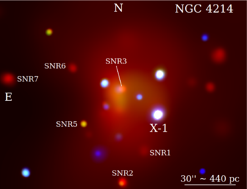
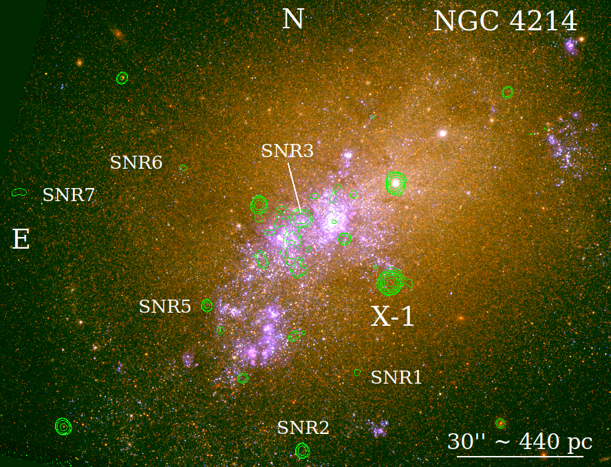
Figure 1: Top Panel: Chandra/ACIS true colour image of NGC 4214, obtained from a stack of all four datasets and then adaptively smoothed. Red = 0.3–1.0 keV, green = 1.0–2.0 keV, blue = 2.0–7.0 keV. X-1 is the subject of this study. SNR1, SNR2, SNR3, SNR5, SNR6, and SNR7 are the X-ray counterparts of the optical SNRs identified by Dopita et al. (2010); their estimated X-ray luminosities are listed in Table 7. Bottom panel: HST/WFC3 UVIS true-color image on the same scale as the Chandra image. Red = F814W ($\approx$I), green = F547M ($\approx$V), blue = F336W ($\approx$U). Chandra flux contours of the strongest X-ray sources are overplotted in green (0.3–7.0 keV band).

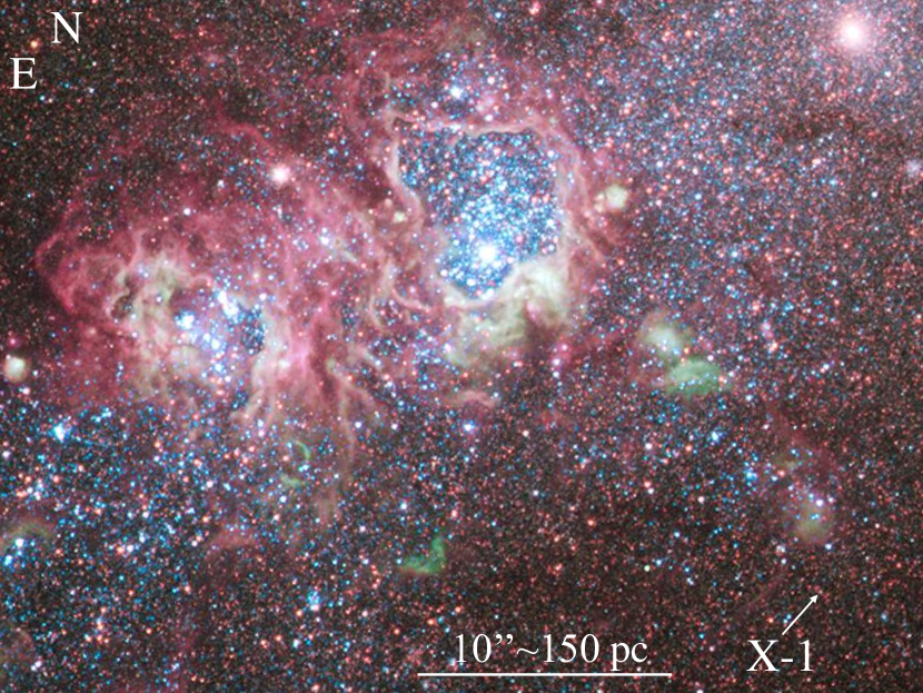
Figure 2: Details of the central region of NGC 4214, adapted from an HST/WFC3 image processed and published by the Hubble Heritage Team (images from the GO-11360 program; PI: R. O’Connell). The red color comes from a combination of the F657N and F814W filters; the green color is from F502N and F547M; the blue color is from F225W, F336W, F438W, and F487N. The optical counterpart of X-1 is marked by an arrow near the bottom right of the image. It is at the outskirts of the current starburst region. Credit: NASA, ESA, and the Hubble Heritage (STScI/AURA)-ESA/ Hubble Collaboration.

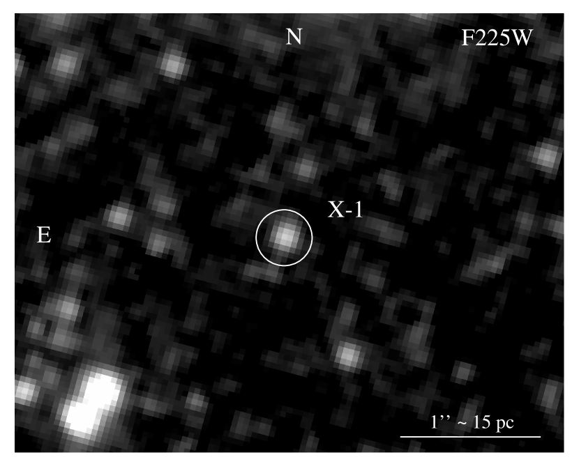
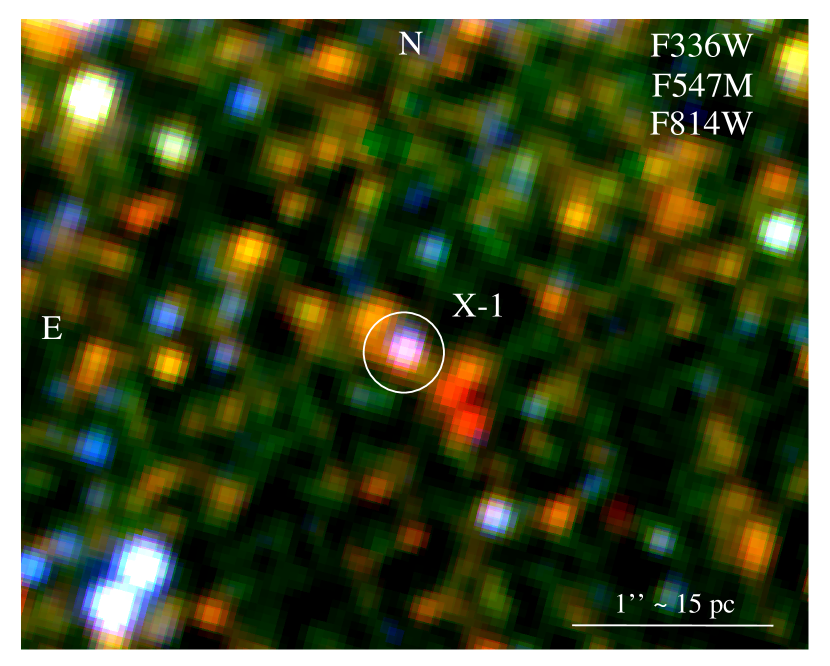
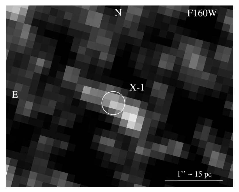
Figure 3: Top Panel: zoomed-in view of the field around X-1 in the near-UV band (HST/WFC3 UVIS filter F225W). The circle has a radius of 0$\farcs$2, approximately corresponding to the positional uncertainty of the X-ray source on the HST image. The image has been smoothed with a Gaussian kernel of radius 2 pixels. Middle panel: HST/WFC3 UVIS true-color image of the same field, also smoothed with a 2-pixel Gaussian. Red = F814W, green = F547M, blue = F336W. Bottom panel: (unsmoothed) HST/WFC3 IR image of the same field (F160W filter).

1.1 Previous studies of NGC 4214 X-1

NGC 4214 (Figures 1,2) is a dwarf starburst galaxy (e.g., MacKenty et al., 2000; Hartwell et al., 2004; Úbeda et al., 2007; McQuinn et al., 2010; Dopita et al., 2010; Williams et al., 2011; Choi et al., 2020) at a distance of $\approx$($3.0\pm 0.1)$ Mpc (Dalcanton et al., 2009; Dopita et al., 2010), corresponding to a distance modulus of $(27.4\pm 0.1)$ mag. It has a current star formation rate $\approx$0.05–0.10 $M_{\odot}$ yr^-1 (Hartwell et al., 2004; McQuinn et al., 2010; Williams et al., 2011), and an average metallicity similar to the Large Magellanic Cloud (Kobulnicky & Skillman, 1996; Williams et al., 2011). Despite its obvious recent burst of star formation, only $\sim$1% of the stellar mass formed in the last 100 Myr, and only $\sim$10% in the last 4 Gyr (Williams et al., 2011); star formation activity appears to have picked up recently, especially over the last $\sim$10 Myr. Thus, its point-source X-ray population may include both HMXBs and low-mass X-ray binaries (LMXBs).

Previous X-ray studies of NGC 4214 with the Chandra X-ray Observatory and XMM-Newton showed (Hartwell et al., 2004; Binder et al., 2015) both diffuse emission from star-forming regions, and point sources (X-ray binaries and supernova remnants (SNRs)). Among the point-source population, the brightest source (CXOU J121538.2$+$361921 = X-1) reaches a peak luminosity of $\approx$10³⁹ erg s^-1 (Ghosh et al., 2006). The most remarkable property of X-1, discovered and discussed in details by Ghosh et al. (2006), is an apparent X-ray eclipse, with a period of 3.62 hr (most likely, the binary period). From their X-ray timing and spectral analysis, Ghosh et al. (2006) argued that the most likely interpretation is a NS or BH accreting from a stripped He star via Roche lobe overflow. The observed binary period implies a donor-star radius $R_{2}\sim 0.5$–$2R_{\odot}$ for plausible ranges of primary masses and mass ratios. An intermediate-mass He star ($M_{2}\lesssim 3$–$4M_{\odot}$) was considered a more likely donor than a classical WR star, because Ghosh et al. (2006) found no evidence of strong winds (no significant changes in neutral absorption and spectral hardness ratio at eclipse ingress/egress). A low-mass main-sequence donor ($M_{2}\sim 0.4M_{\odot}$) would have been consistent with the short binary period but not with the apparently persistent nature of the X-ray source over several years. However, the non-detection of an optical counterpart made it impossible to provide stronger constraints.

Table 2: Log of the Chandra/ACIS observations of X-1. Offset values indicate the off-axis distance of X-1 in each observation. Count rates are observation-averaged background-subtracted values in the 0.3–8 keV band.

ObsID	Date	Start Time	Exp.	Offset	Count Rate
		(MJD)	(ks)		($10^{-3}$ ct s-1)
2030	2001-10-16	52198.7957	26.4	1$\farcm$9	$35.7\pm 1.2$
4743	2005-04-07	53098.1970	27.2	2$\farcm$0	$7.1\pm 0.5$
5197	2005-08-03	53216.3293	28.6	1$\farcm$9	$29.6\pm 1.0$
22372	2020-08-01	59062.4143	59.3	0$\farcm$1	$22.0\pm 0.6$

Table 3: HST/WFC3 observations of X-1 used for this study. The dataset in the F275W filter was taken on 2022 November 14; all the others are from 2009 December 22–25.

Filter	Exp	$\lambda_{\rm eff}$	Brightness	Flux Density
	(s)	(Å)	(Vegamag)	(erg cm-2 s-1 Å-1)
F225W	1665	2372.1	$22.54\pm 0.06$	$(4.1\pm 0.2)\times 10^{-18}$
F275W	2380	2709.7	$22.75\pm 0.08$	$(3.0\pm 0.2)\times 10^{-18}$
F336W	1683	3354.6	$23.16\pm 0.03$	$(1.79\pm 0.03)\times 10^{-18}$
F438W	1530	4325.7	$24.50\pm 0.05$	$(1.07\pm 0.05)\times 10^{-18}$
F547M	1050	5447.5	$24.09\pm 0.05$	$(0.87\pm 0.05)\times 10^{-18}$
F657N	1592	6566.6	NA	$(0.76\pm 0.11)\times 10^{-18}$
F673N	2940	6765.9	NA	$(0.99\pm 0.06)\times 10^{-18}$
F814W	1339	8039.1	$22.44\pm 0.05$	$(1.20\pm 0.05)\times 10^{-18}$
F110W	1197	11534.5	$21.07\pm 0.05$	$(1.50\pm 0.07)\times 10^{-18}$
F160W	2397	15369.2	$20.1\pm 0.1$	$(1.3\pm 0.1)\times 10^{-18}$

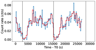
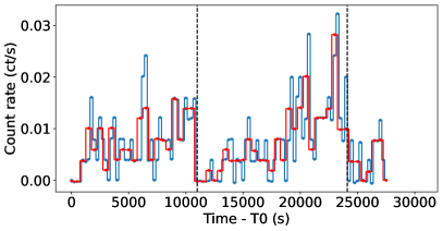
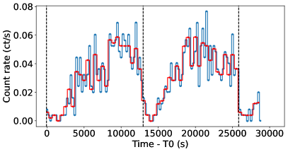
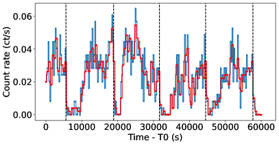
Figure 4: Chandra/ACIS light curves of X-1 in the 0.3–8 keV band. Top left: ObsIDs 2030; top right: ObsID 4743; bottom left: ObsIDs 5197; bottom right: ObsID 22372. Each light curve has been rebinned to 250 s (blue histogram) and 500 s (red histogram). Dashed black lines mark the 250 s bins corresponding to eclipse ingresses. The last dashed line in ObsID:2030 and first dashed line in ObsID:5197 are predicted eclipse times. In each plot, the reference time $T_{0}$ is the observation start time in Table 2. We have omitted the error bars for clarity.

1.2 Specific objectives of our new study

We carried out a follow-up optical/X-ray study of NGC 4214 X-1. Our main specific objectives are: a) to identify a candidate optical counterpart in a set of Hubble Space Telescope (HST) observations that were not available at the time of the previous investigation, and verify whether the optical brightness is consistent with the suggested scenarios; b) to determine whether the source is still in a X-ray bright state, two decades after the first Chandra observations, and/or whether there is evidence of state transitions; c) to determine the duration and average ingress/egress profiles of the X-ray eclipses more accurately; d) to determine whether the X-ray spectrum is dominated by a thermal (disk-blackbody) or a non-thermal (power-law) component.

To achieve those objectives, we have combined the three archival Chandra datasets from 2001–2005 with new data taken on 2020 August 1 (ObsID 22372, PI: R. Soria). We have also used archival HST Wide Field Camera 3 (WFC3) images taken on 2009 December 22–25 (Program ID 11360, PI: R. O’Connell) and 2022 November 14 (Program ID 17225, PI: D. Calzetti). A summary of the Chandra and HST observations is presented in Tables 2 and 3.

In Section 2, we summarize our X-ray and optical data analysis procedures, and report on the improved astrometry, which enables the identification of a likely optical counterpart. In Sections 3 and 4, we present the results of X-ray lightcurve and spectral modelling, respectively. In Section 5, we report on the optical brightness and colors. Finally, we discuss the implications of such results for the system parameters in Section 6.

2 Methods

2.1 Chandra data analysis

In all four Chandra observations (Table 2), X-1 was located in the S3 chip of the Advanced CCD Imaging Spectrometer (ACIS) camera. After downloading the data from the public archives, we reprocessed them with the Chandra Interactive Analysis of Observations (ciao) software version 4.13 (Fruscione et al., 2006), Calibration Database 4.9.5. We created new level-2 event files with the ciao tasks chandra_repro. For each observation, we visually inspected the light curve of a large background region, binned at 250 s and 500 s time bins, to search for flares. We found an $\sim$4 ks interval at the end of ObsID 4743 of strong flaring but determined that only a few extra background events (no more than 8.5% of the total source$+$background counts) can be attributed to this activity, which occurred during an eclipse (hence, maximizing the background contribution to the total counts in the source region). We did not exclude this flare interval, preferring instead to retain the longest possible continuous time intervals to better conduct our searches for periodic signals.

We applied a barycenter correction with axbary, for timing analysis. We used reproject_obs to create stacked images, dmextract to obtain lightcurves from each observation, and srcflux for preliminary count rate and flux estimates. We then used specextract to create spectra and associated response and ancillary response files. For timing and spectral analysis, we used source extraction circles of $3^{\prime\prime}$ radius, centered using the centroid command in ds9, in each of the four observations. Local background annuli were centered on the same coordinates as the source region with an inner radius of $4^{\prime\prime}$ and an outer radius of at least $17^{\prime\prime}$.

We used NASA’s High Energy Astrophysics Science Archive Research Center (HEASARC) software for further data analysis; in particular, the ftools package (Blackburn, 1995; Nasa High Energy Astrophysics Science Archive Research Center (2014), Heasarc). With ftools’s grppha task, we regrouped the spectra to a minimum number of counts per bin, suitable for spectral fitting: $\geq$1 count per bin for the Cash statistics (Cash, 1979) and $\geq$15 counts per bin for the $\chi^{2}$ statistics. We fitted the spectra with xspec, version 12.12.0 (Arnaud, 1996), over the standard 0.3–8 keV ACIS energy range. We tested all the models used in this study both on the minimally grouped spectra with the cstat fit statistic (Cash, 1979), and on the more grouped version of the same spectra with the $\chi^{2}$ statistics, whenever possible (i.e., for spectra with enough counts). In all those cases, our results are consistent between the two fitting statistics, as expected because of the asymptotic equivalence of the Poisson and Gaussian statistics. The spectrum from ObsID 4743 (Section 4.1) and some of the low-flux-threshold spectra (Section 4.2) do not have enough counts for $\chi^{2}$ fitting (i.e., the regrouped spectra have only $\sim$10 bins and substantially undersample the spectral resolution, with a loss of information). Such spectra are better fitted with the cstat statistic. For consistency, we report all the best-fitting parameter values, fluxes and confidence intervals obtained with cstat. Model absorbed and unabsorbed fluxes were obtained with the cflux convolution model. Uncertainties for one interesting parameter (calculated with the steppar command) are reported at the confidence interval of $\Delta C=\pm$2.70: this is asymptotically equivalent to the 90% confidence interval in the $\chi^{2}$ statistics.

2.2 HST data analysis and refined astrometry

NGC 4214 was observed by HST/WFC3 on 2009 December 22–25, in several broad-band and narrow-band filters; those used for this study are listed in Table 3. An additional HST/WFC3 observation in the F275W filter was taken on 2022 November 14. We downloaded the drizzled, calibrated HST/WFC3 image files (.drc files for WFC3-UVIS, .drz files for WFC3-IR) from the Mikulski Archive for Space Telescopes. We used the ds9 analysis tools for astrometry and photometry. Comparing the Chandra and HST images, we found at least nine X-ray sources with likely matches on the HST images. Six of them (Figure 1) are supernova remnants previously identified by Dopita et al. (2010) in the narrow-band images. They are extended in the HST images, and barely above the detection limit in the Chandra images. Thus, those sources are not useful to improve the relative astrometry of Chandra and HST images beyond an $\approx$0$\farcs{5}$ uncertainty. Another three Chandra sources correspond to point-like sources in the HST broad-band images. For those three associations, we measured an average offset of $0\farcs{14}$ and a maximum offset of $0\farcs{21}$. We applied a simple translation of the Chandra wcs coordinate system using the ciao utility wcs_update to align the Chandra data to the HST coordinates. We do not have enough Chandra/HST associations to justify more complex transformations such as rotation and scaling. As for the HST absolute astrometry, we did not detect any systematic offset between matching sources in HST, SDSS, and Gaia.

Combining the uncertainty in the centroid of the X-ray source on the ACIS chip with the uncertainty in the relative astrometric alignment of Chandra and HST, we estimate a 90% confidence radius of $\approx$0$\farcs{2}$ for the location of X-1 on the HST images. We find that there is only one point-like optical candidate in the Chandra error circle of X-1 (in fact, right at the centre). The candidate point-like optical counterpart is also the brightest blue object within $\approx$30 pc of the X-ray position (Figure 3). In summary, the coordinates of X-1 are R.A.(J2000) $=12^{h}15^{m}38^{s}.25(\pm 0^{s}.01)$, Dec(J2000) $=+36^{\circ}19^{\prime}21\farcs{0}(\pm 0\farcs{1})$.

To estimate the flux from the candidate HST counterpart, we used standard ds9 aperture photometry tools. Specifically, we defined a source circle of radius $0\farcs{16}$ for the WFC3-UVIS images (optical/UV) and $0\farcs{20}$ for the WFC3-IR images (near-infrared). The circle was centred on the optical centroid of the HST counterpart (estimated with the centroid tool in ds9); that position is also within a single WFC3-UVIS pixel of the Chandra position. In each image, we selected and averaged three local background regions with a combined area of about twelve times the source circle. Such regions were suitably placed to avoid the bright stars north-east and south-west of X-1. We repeated the background estimation several times for each image, with different placements and relative sizes of the background regions, and took the median value of the aperture-limited net count rate. The dispersion in the net count rate values for different background locations gave us an estimate of the uncertainty, more comprehensive than an estimate based on Poisson statistics of the number of detected electrons. We converted aperture-limited count rates to infinite-aperture values $\rm{CR_{inf}}$, using the online tables of encircled energy fractions. We then obtained magnitudes and flux densities from the infinite-aperture count rates, using the latest tables of UVIS zeropoints and IR zeropoints, with the standard relation

$${m_{\rm vega}}=-2.5\times\log_{10}(\rm{CR_{inf}})+\rm{ZP_{vega}},$$ (1)

where $m_{\rm vega}$ is the apparent magnitude in the VegaMag system and $\rm{ZP_{vega}}$ is the corresponding zeropoint. Finally, we converted each WFC3 datapoint (in flux density units) to pha $+$ rsp file format, suitable to xspec modelling. This is a standard technique that allows joint fitting of X-ray and optical data. For this, we used the ftools task ftflx2xsp.

3 X-ray timing results

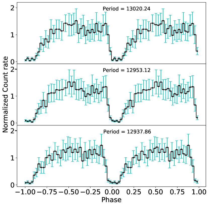
Figure 5: Average Chandra light-curve of X-1 in the 0.3–8 keV band, folded on three alternative and statistically equivalent binary periods, and rebinned to 35 phase intervals per period. Top panel: folding period of 13020.24 s; middle panel: folding period of 12953.12 s; bottom panel: folding period of 12937.86 s.

3.1 Period searching

Before searching for the best-fitting period, we renormalized the Chandra light curves of X-1 to the average net count rate in each observation. We did this to correct for the decreasing sensitivity of ACIS-S in more recent epochs, which would have biased the period search in favour of the earlier observations.

First, we applied ftools’s efsearch task to the full light curve (all four epochs). The best-fitting period depends both on the time binning of the light curve, and on the time resolution used for period searches. The search is also hampered by the large gaps between epochs. We folded several candidate best-fitting solutions with the efold task and visually inspected them. We find that the most stable solution (obtained with 500 s binning of the light curves and 0.01 s period search resolution) is at $P\approx 13020.24$ s. The corresponding folded light curves is shown in the top panel of Figure 5.

To test this value and perhaps obtain a more robust estimate, we took advantage of the 11 X-ray eclipses covered by our observations (Figure 4). At all four epochs, eclipse ingresses are typically sharper than the corresponding egresses. Thus, we used ingress times to determine the best-fitting period. For each eclipse, we defined the ingress time $t_{e}$ as the mid-point of the 250 s bin with the largest count-rate drop, and attribute an uncertainty of $\pm 125$ s to that datapoint, for period searching.

We used a least-squares algorithm to fit a linear function to the cycle numbers and times of eclipse ingress:

$$t_{e}=I\times P+T_{0},$$ (2)

where $I$ is the cycle number, $P$ is the orbital period, and $T_{0}$ is a reference eclipse ingress time. We obtained a best-fitting period $P=12937.86\pm 267.21$ s. Of the four Chandra epochs, ObsID 4743 is when the source was faintest, and it is more difficult to pinpoint the ingress times of its two eclipses with the same confidence as for the other 9 events. To test whether this may affect our period search, we repeated our fitting without ObsID 4743. We obtained a period $P=12953.12\pm 245.98$ s. The $\sim$$\pm$250 s error range of the best-fitting period is the envelope within which we find acceptable folding solutions; it does not mean that any period within that time range is equally likely. Instead, there is a discrete list of acceptable periods, each of them corresponding to a different, integer number of orbital cycles elapsed from the first to the last observation. Given that the observations span 20 years, and there are gaps of many years between them, it is unfortunately impossible to unequivocally phase-connect the light-curves.

3.2 Eclipse Profile

Regardless of the choice of folding period, the folded eclipse profile has a faster (though not instantaneous) ingress and a slower egress, lasting as long as $\sim$0.3 times the binary period before the flux returns to the out-of-eclipse level. The eclipse itself is well defined in the average light-curve (Figure 5) although it can be difficult to define in individual observations, because of the difficulty to determine when the true eclipse ends and the slow egress begins. This “fuzziness” is usually a sign that the eclipsing donor star is surrounded by a dense wind; we will discuss this issue later.

Based on the average light-curve, we estimate an eclipse duration $\Delta T_{\rm ecl}\approx 2050\pm 175$ s. Among the individual eclipses observed in the four epochs, the one with the sharpest ingress and egress (which we interpret as the epoch in which the effect of the wind was least important) was the second eclipse in ObsID 22372: in that case, too, the duration was $\approx$2000 s. Thus, we shall use this average value for an estimate of the size of the donor star. Correspondingly, the eclipse fraction $\Delta_{\rm ecl}\equiv\Delta T_{\rm ecl}/P=0.158\pm 0.014$.

Table 4: Best-fitting absorbed power-law model of the Chandra/ACIS spectra of X-1 in the four epochs. The spectra were fitted with the Cash statistics. The Galactic column density was fixed at $N_{\rm{H,Gal}}=4\times 10^{20}$ cm^-2. Error ranges are 90% confidence limits for one interesting parameter.

Model Parameters	Values in Each ObsID
	2030	4743	5197	22372
$N_{\rm{H,int}}$ ($10^{21}$ cm-2)	$1.4^{+0.5}_{-0.5}$	$<1.2$	$2.0^{+0.7}_{-0.6}$	$2.5^{+1.3}_{-1.2}$
$\Gamma$	$1.77^{+0.16}_{-0.15}$	$2.19^{+0.41}_{-0.27}$	$1.84^{+0.17}_{-0.16}$	$1.95^{+0.16}_{-0.15}$
$N_{\rm{po}}^{a}$	$5.8^{+0.9}_{-0.7}$	$1.1^{+0.4}_{-0.2}$	$5.8^{+0.9}_{-0.9}$	$8.5^{+1.6}_{-1.4}$
C-stat/dof	$229.1/331$ (0.69)	$86.1/115$ (0.75)	$193.0/261$ (0.74)	$327.2/322$ (1.02)
$f_{0.3-8}$ ($10^{-13}$ erg cm-2 s-1)b	$2.7^{+0.3}_{-0.2}$	$0.46^{+0.08}_{-0.08}$	$2.4^{+0.3}_{-0.2}$	$3.1^{+0.2}_{-0.2}$

Note. — ^a: units of $10^{-5}$ photons keV^-1 cm^-2 s^-1 at 1 keV.

^b: observed flux in the 0.3–8 keV band

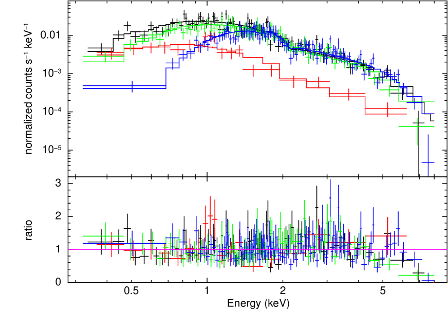
Figure 6: Chandra/ACIS-S spectra of X-1 in the four epochs of observations, with best-fitting power-law model and data/model ratios. Black datapoints and model histogram are for ObsID 2030; red for ObsID 4743; green for ObsID 5197; blue for ObsID 22372. See Table 4 for the fit parameters. The spectra were fitted with the Cash statistics; the datapoints have been rebinned to a signal-to-noise ratio $>$3 for plotting purposes only. The decreasing count rates below 1 keV from the black to the green and blue spectra are the result of the decrease of ACIS-S sensitivity from 2001 to 2020, for the same absorbing column density.

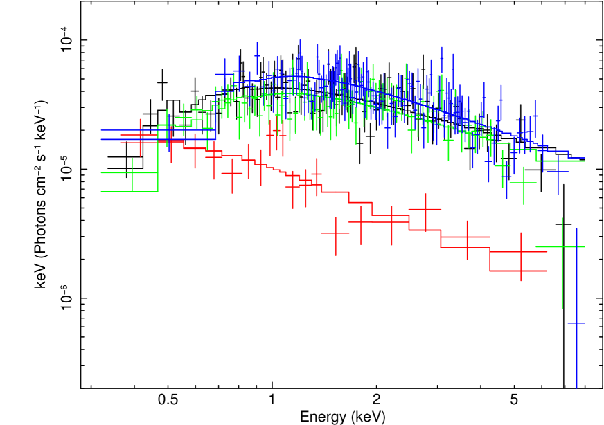
Figure 7: Unfolded Chandra/ACIS-S spectra of X-1 in the four epochs of observations, based on a power-law model (Table 4). Color coding and re-binning are as in Figure 6. The unfolded spectra highlight that X-1 was in a different state in ObsID 4743, compared with the other three epochs.

4 X-ray spectral results

4.1 Thermal and non-thermal components

To begin, we compared the four spectra corresponding to the four Chandra observations, without any other selection criteria. We used a simple power-law model, absorbed with a Galactic line-of-sight component plus an intrinsic component (tbabs_Gal $\times$ tbabs_int $\times$ pow). The foreground column density was fixed at $N_{\rm H}=4\times 10^{20}\;\rm{cm^{-2}}$ (HI4PI Collaboration et al., 2016), while the intrinsic column was left as a free parameter. The purpose of this initial exercise was simply to assess whether the source was in a similar spectral state during the four epochs. We found that an absorbed power-law is a decent fit for each of the four epochs (Figure 6 and Table 4); there are hints of a systematic curvature and high-energy turnover in the residuals, but they are not statistically significant in individual spectra, given their moderately low signal to noise level. In three of the four epochs, the observed spectra have similar slopes and normalizations (Figure 6); the difference in the observed spectral shapes at low energies is only due to the loss of sensitivity of the ACIS-S detector over the years. The only epoch with a clearly different spectral shape is ObsID 4743 (red data points and model in Figures 6, 7), with a softer power-law slope and lower luminosity.

Based on those preliminary results, we built a combined spectrum of ObsIDs 2030, 5197 and 22372 (leaving out ObsID 4743, as explained above). This was done with the combine_spectra script in the ciao tool specextract, which creates exposure-weighted arf files, and arf-weighted response files. We found that an absorbed disk-blackbody model (Figure 8, Table 5) is a better fit than an absorbed power-law (C-statistics of 338.8 for 380 degrees of freedom for the disk model, compared with 375.4/380 for the power-law model). The inner-disk radius $R_{\rm in}$, estimated from the disk normalization (Kubota et al., 1998), depends on the viewing angle $\theta$. Given the presence of eclipses, we know that the binary orbital plane is seen at high inclination, $i\gtrsim 70^{\circ}$; we assume that the X-ray emitting part of the disk is aligned with the orbital plane ($\theta\approx i$), in the absence of specific evidence against this simplified scenario. For example, for $\theta=75^{\circ}$, $R_{\rm in}\approx 45$ km, and for $\theta=80^{\circ}$, $R_{\rm in}\approx 55$ km (Table 5). These are typical values found in stellar-mass BH X-ray binaries in the high/soft state (McClintock et al., 2014; Remillard & McClintock, 2006). For disk emission, the relation between flux and luminosity is also a function of viewing angle: $L_{\rm X}\approx 2\pi d^{2}f_{\rm X}/(\cos\theta)$. For $\theta=75^{\circ}$, we estimate a 0.3–10 keV luminosity $L_{\rm X}\approx 5.8\times 10^{38}$ erg s^-1, and for $\theta=80^{\circ}$, $L_{\rm X}\approx 8.6\times 10^{38}$ erg s^-1 km. Considering that such values include part of the exposure time in which the source was in eclipse ingress/egress, we conclude that the intrinsic X-ray luminosity out of eclipse is close to $\approx$10³⁹ erg s^-1, Eddington limit of a stellar-mass BH. The best-fitting peak color temperature $kT_{\rm in}\approx(1.3\pm 0.1)$ keV is also consistent with the temperatures observed at the peak of the high/soft state (near their Eddington limit) in Galactic stellar-mass BH transients (Kubota & Makishima, 2004; Abe et al., 2005; Sutton et al., 2017).

Next, we tried more complex fitting models for the combined three-ObsID spectrum: i) a standard disk-blackbody plus power-law model; ii) a disk model with a free power law dependence of the color temperature on radius, $T\propto R^{-p}$ (diskpbb in xspec, generally used as a simple approximation of super-critical slim-disk models); iii) a Comptonization model (simpl $\times$ diskbb). None of those models provides a statistically significant improvement to the diskbb model. Finally, we tried adding an ionized absorber (absori model) but found no statistical need for it. When the ionization parameter in absori is frozen to its maximum value of 1000, we can only determine an upper limit to the possible ionized column density, $N_{\rm H}^{\rm ion}<3.3\times 10^{22}$ cm^-2 at the 90% confidence level.

We modelled the spectrum from ObsID 4743 separately. We tried adding an optically thin thermal plasma (apec) component (Figure 9 and Table 6) to the pure power law model, justified by the residuals seen around 1 keV. Using the task simftest in xspec, we found a statistical improvement at the 99% confidence level over the simple power-law model (C-statistics of 74.9 for 113 degrees of freedom, and 83.0/115, respectively). Conversely, we verified that the same apec component would not be statistically significant in the other three epochs, because of their higher continuum flux.

Table 5: Best-fitting parameters of the combined Chandra/ACIS spectrum from ObsIDs 2030, 5197, 22372, fitted with the Cash statistics. The model is tbabs_Gal $\times$ tbabs_int $\times$ diskbb. The Galactic column density was fixed at $N_{\rm{H,Gal}}=4\times 10^{20}$ cm^-2. Error ranges are 90% confidence limits for one interesting parameter.

Model Parameters	Values
$N_{\rm{H,int}}$ ($10^{20}$ cm-2)	$<2.9$
$kT_{\rm in}$ (keV)	$1.33^{+0.07}_{-0.07}$
$N_{\rm{dbb}}$ ($10^{-3}$ km2)a	$4.3^{+0.9}_{-0.7}$
$R_{\rm{in}}\sqrt{\cos\theta}$ (km)b	$23.5^{+2.4}_{-2.1}$
C-stat/dof	$338.8/380$ (0.89)
$f_{0.3-8}$ ($10^{-13}$ erg cm-2 s-1)c	$2.60^{+0.05}_{-0.10}$
$L_{0.3-10}\cos\theta$ ($10^{38}$ erg s-1)d	$1.50^{+0.06}_{-0.06}$

Note. — ^a: $N_{\rm{dbb}}=(r_{\rm{in}}/d_{10})^{2}\cos\theta$, where $r_{\rm{in}}$ is the “apparent” inner disk radius in km, $d_{10}$ the distance to the galaxy in units of 10 kpc (here, $d_{10}=300$), and $\theta$ is our viewing angle to the disk surface. The bolometric luminosity of the disk is $L\approx 4\pi r_{\rm{in}}^{2}\,\sigma T_{\rm{in}}^{4}$ (Makishima et al., 1986);

^b: the “true” inner-disk radius $R_{\rm{in}}$ is defined as $R_{\rm{in}}\approx 1.19\,r_{\rm in}$ for a standard disk (Kubota et al., 1998), and $r_{\rm{in}}$ was defined in Table note d;

^c: observed flux in the 0.3–8 keV band;

^d: $L_{0.3-10}$ is the un-absorbed luminosity in the 0.3–10 keV band, defined as $2\pi d^{2}/(\cos\theta)$ times the un-absorbed 0.3–10 keV model flux.

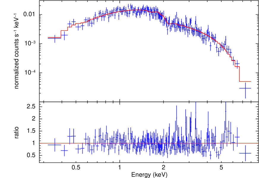
Figure 8: Combined Chandra/ACIS-S spectrum of X-1 from ObsIDs 2030, 5197 and 22372, with best-fitting diskbb model and data/model ratios. See Table 5 for the fit parameters. The spectra were fitted with the Cash statistics; the datapoints have been rebinned to a signal-to-noise ratio $>$3 for plotting purposes only.

Table 6: Best-fitting parameters of the Chandra/ACIS spectrum from ObsIDs 4743, fitted with the Cash statistics. The model is tbabs_Gal $\times$ tbabs_int $\times$ (pow $+$ apec). The Galactic column density was fixed at $N_{\rm{H,Gal}}=4\times 10^{20}$ cm^-2. Error ranges are 90% confidence limits for one interesting parameter.

Model Parameters	Values
$N_{\rm{H,int}}$ ($10^{20}$ cm-2)	$<4.5$
$\Gamma$	$1.98^{+0.29}_{-0.29}$
$N_{\rm{po}}^{a}$	$7.8^{+2.4}_{-2.1}$
$kT_{\rm apec}$ (keV)	$1.20^{+0.34}_{-0.23}$
$N_{\rm{apec}}^{b}$	$\left(5.2^{+5.4}_{-3.4}\right)\times 10^{-6}$
C-stat/dof	$74.9/113$ (0.66)
$f_{0.3-8}$ ($10^{-14}$ erg cm-2 s-1)c	$4.5^{+0.8}_{-0.7}$
$L_{0.3-10}$ ($10^{37}$ erg s-1)d	$5.7^{+1.0}_{-0.9}$

Note. — ^a: units of $10^{-6}$ photons keV^-1 cm^-2 s^-1 at 1 keV.

^b: $N_{\rm{apec}}\equiv\left[10^{-14}/\left(4\pi d^{2}\right)\right]\,\int n_{e}n_{\rm H}\,dV$, where $d$ is the luminosity distance in cm, and $n_{e}$ and $n_{\rm H}$ are the electron and H densities in cm^-3.

^c: observed flux in the 0.3–8 keV band

^d: un-absorbed 0.3–10 keV luminosity, defined as $4\pi d^{2}$ times the un-absorbed 0.3–10 keV model flux.

4.2 Flux-resolved spectral modelling

The next step of our spectral analysis is flux-resolved modelling. We want to determine whether and how the spectral shape changed between the higher-luminosity time bins and the eclipse ingress/egress time bins. Our first working hypothesis we shall test is that the accretion column (including both neutral and ionized gas) is higher immediately before and after the eclipses; we may also see a spectral change if different X-ray emission components come from different regions in the binary system, and some are more occulted or absorbed than others around an eclipse. For this objective, we include again ObsIDs 2030, 5197 and 22372, and leave out ObsID 4743, to avoid mixing different spectral states.

In order to define a physically consistent count-rate threshold for the three epochs, we need to account for the decrease in ACIS-S sensitivity over the years. Based on the best-fitting diskbb model of the combined spectrum (Section 4.1), we estimate that 1 ct/ks in ObsID 2030 corresponds to 0.828 ct/ks in ObsID 5197 and 0.618 ct/ks in ObsID 22372. After binning the lightcurve to 500-s intervals, we defined various count-rate thresholds. For each threshold, we extracted and modelled two combined spectra from all the bins above and all those below that threshold. We report here the results for three choices of threshold: $10^{-2}$ ct s^-1 in ObsID 2030 (corresponding to $8.28\times 10^{-3}$ ct s^-1 and $6.18\times 10^{-3}$ ct s^-1 in the other two epochs); $2\times 10^{-2}$ ct s^-1 ($1.66\times 10^{-2}$ ct s^-1 and $1.24\times 10^{-2}$ ct s^-1, respectively); $3\times 10^{-2}$ ct s^-1 ($2.48\times 10^{-2}$ ct s^-1 and $1.85\times 10^{-2}$ ct s^-1, respectively). Other choices of thresholds lead to qualitatively similar results.

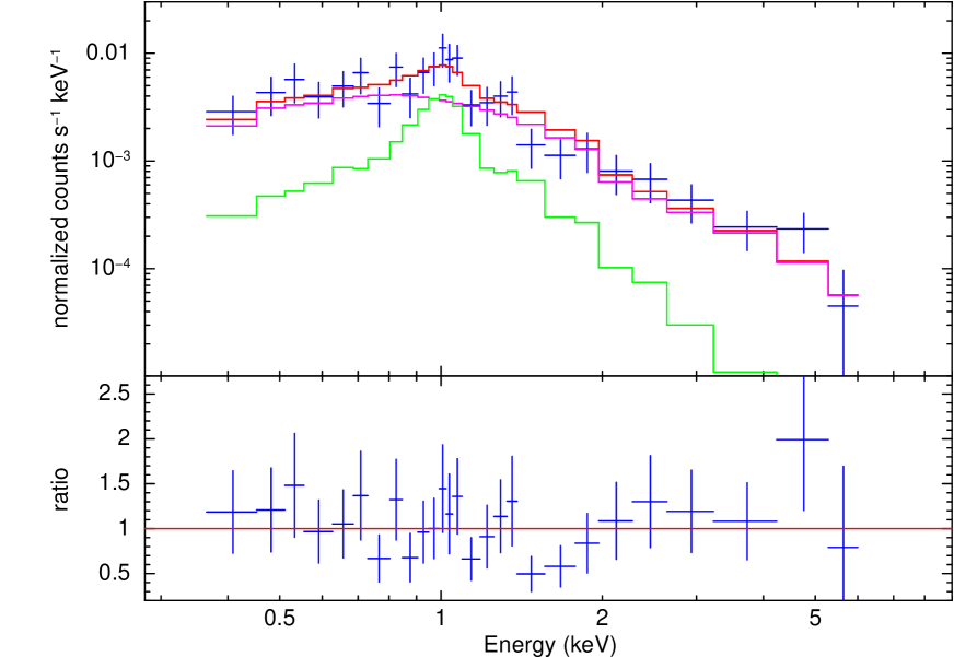
Figure 9: Chandra/ACIS-S spectrum of X-1 from ObsID 4743, with best-fitting pow $+$ apec model and data/model ratios. See Table 6 for the fit parameters. The spectra were fitted with the Cash statistics; the datapoints have been rebinned to a signal-to-noise ratio $>$3 for plotting purposes only. The green histogram shows the contribution of the apec component; the magenta histogram represents the power-law component; the red histogram shows the combined model.

The surprising result is that for any threshold, the difference between the higher and lower flux spectra is simply a constant scaling factor. There is no significant change of spectral shape, and no change in photoelectric absorption ($N_{\rm H}$ in the tbabs component), which would have removed preferentially soft photons. The two spectra of each pair are well modelled simultaneously with the same diskbb continuum, and a free partial-covering absorber (tbabs_Gal $\times$ tbabs_int $\times$ pcfabs $\times$ diskbb in xspec). The column density in the pcfabs component is constrained to be $>$10²⁴ cm^-2 at the 90% confidence level, which means a completely opaque absorber in the Chandra band. Thus, this is identical to simply placing a constant scaling factor in front of the diskbb component. Specifically, for the 0.01 ct s^-1 threshold (Figure 10, left panel), the low-flux spectrum is absorbed by a Compton-thick medium with a covering fraction of $(91\pm 2)$%, while the covering fraction for the high-flux spectrum is assumed to be zero. The fit statistics is C-stat $=658.4/786$. For the 0.02 ct s^-1 threshold, we obtain a covering fraction of $(84\pm 2)$% for the low-flux spectrum (combined fit statistics C-stat $=776.8/87$). For the 0.03 ct s^-1 threshold (Figure 10, right panel), the covering fraction for the low-flux spectrum is $(76\pm 2)$% (C-stat $=825.7/874$).

A by-product of this exercise is that, by lifting the threshold level, we can estimate the average out-of-eclipse luminosity. We obtain an unabsorbed 0.3–10 keV luminosity $L_{\rm X}\cos\theta\approx 2.3\times 10^{38}$ erg s^-1, which corresponds to $L_{\rm X}\approx 9\times 10^{38}$ erg s^-1 at $\theta=75^{\circ}$ and $L_{\rm X}\approx 1.3\times 10^{39}$ erg s^-1 at $\theta=80^{\circ}$.

It has been known since the early days of X-ray astronomy (e.g., Mason et al. 1985) that an observed decrease in flux without substantial change in hardness and shape is usually caused either by a variable covering fraction in a clumpy medium (i.e., an inhomogeneous medium with Compton thick clouds that cover only part of an extended X-ray emitting region), or by a highly ionized medium (no or few metal absorption lines and edges, with an approximately grey opacity dominated by Thomson scattering). Therefore, we also tried including a multiplicative ionized absorber component, absori, fitting the lower-flux and higher-flux spectral pairs with tbabs_Gal $\times$ tbabs_int $\times$ absori $\times$ diskbb models. Here, we allowed the column density of the absori component to vary between the two spectra of each pair, while all the other parameters were tied. We tried different ionization levels, up to $\xi=5000$ (hard limit in xspec). However, the resulting fits are significantly worse than in the partial covering model, with strong systematic residuals. For example, for the pair of spectra above and below the equivalent ObsID-2030 count rate of 0.03 ct s^-1, the best-fitting absori model at $\xi=5000$ has a C-statistic of 900.5 for 876 degrees of freedom, compared with 825.7/874 for the partial covering model. Extrapolating the absori model beyond the xspec limit, we estimate that we need an ionization parameter $\xi\gtrsim 10^{4}$ to reproduce the featureless decrease in flux seen in the data.

Finally, we replaced absori with the optically-thin Compton scattering model cabs, which accounts for the scattering of a fraction of X-ray photons out of the beam (model: tbabs_Gal $\times$ tbabs_int $\times$ cabs $\times$ diskbb). cabs attenuates the observed flux by a factor $\exp{\left[-N_{\rm H}\sigma_{\rm T}(E)\right]}$, where $\sigma_{\rm T}(E)$ is the Thomson cross section with Klein-Nishina corrections (essentially a constant over the Chandra/ACIS band). Fitting the spectrum with a cabs attenuation factor is formally equivalent to fitting a partial-covering fraction of a Compton-thick absorber, or simply multiplying the model by a free constant. As expected, we obtain statistically identical fits with cabs and pcfabs (Figures 10). Specifically, for the 0.01 ct s^-1 threshold, the column density of the scattering medium is $N_{\rm H}=(3.0\pm 0.3)\times 10^{24}$ cm^-2 for the low-flux spectrum, while $N_{\rm H}\equiv 0$ for the high-flux spectrum (C-stat $=658.4/786$). For the 0.02 ct s^-1 threshold, the scattering $N_{\rm H}=(2.3\pm 0.2)\times 10^{24}$ cm^-2 (C-stat $=776.8/875$). For the 0.03 ct s^-1 threshold, $N_{\rm H}=(1.8\pm 0.1)\times 10^{24}$ cm^-2 (C-stat $=825.7/874$).

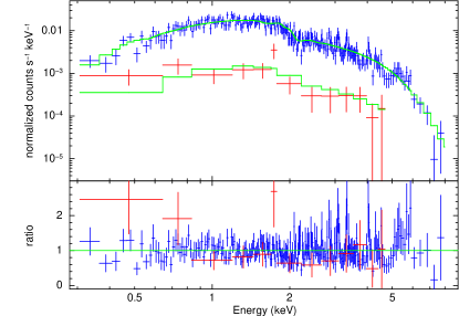
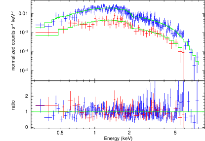
Figure 10: Left panel: Chandra/ACIS-S spectra above (blue datapoints) and below (red datapoints) a threshold corresponding to an equivalent count rate of 0.01 ct s^-1 in ObsID 2030. The spectra were simultaneously fitted with the Cash statistics; the datapoints have been rebinned to a signal-to-noise ratio $>$2.7 for plotting purposes. The fitted model is tbabs_Gal $\times$ tbabs_int $\times$ pcfabs $\times$ diskbb, with all parameters locked between the two spectra except for the covering fraction in pcfabs. The best-fitting covering fraction in the low-flux spectrum is $(91\pm 2)$% (C-stat $=658.4/786$). A formally identical fit is obtained with the pure Compton scattering model cabs, which implies a column density of the scattering medium $N_{\rm H}=(3.0\pm 0.3)\times 10^{24}$ cm^-2 in front of the low-flux spectrum. Right panel: as in the left panel, for a threshold corresponding to an equivalent count rate of 0.03 ct s^-1 in ObsID 2030. The best-fitting partial-covering fraction is $(76\pm 2)$% for the low-flux spectrum. Alternatively, a Compton scattering model implies $N_{\rm H}=(1.8\pm 0.1)\times 10^{24}$ cm^-2 (C-stat $=825.7/874$ in both models).

5 Optical results

The point-like optical counterpart stands out as one of the brightest sources within a few 10s of pc of the X-1 position (Figure 3), both in the near-UV and in the near-IR, but is relatively faint in the $V$ band (Table 3). An approximate conversion to standard colors indicates $U-B\approx-1.2$ mag, and $V-I\approx 1.6$ mag. There are no stars with this type of bimodal colors, which are inconsistent with any single thermal model.

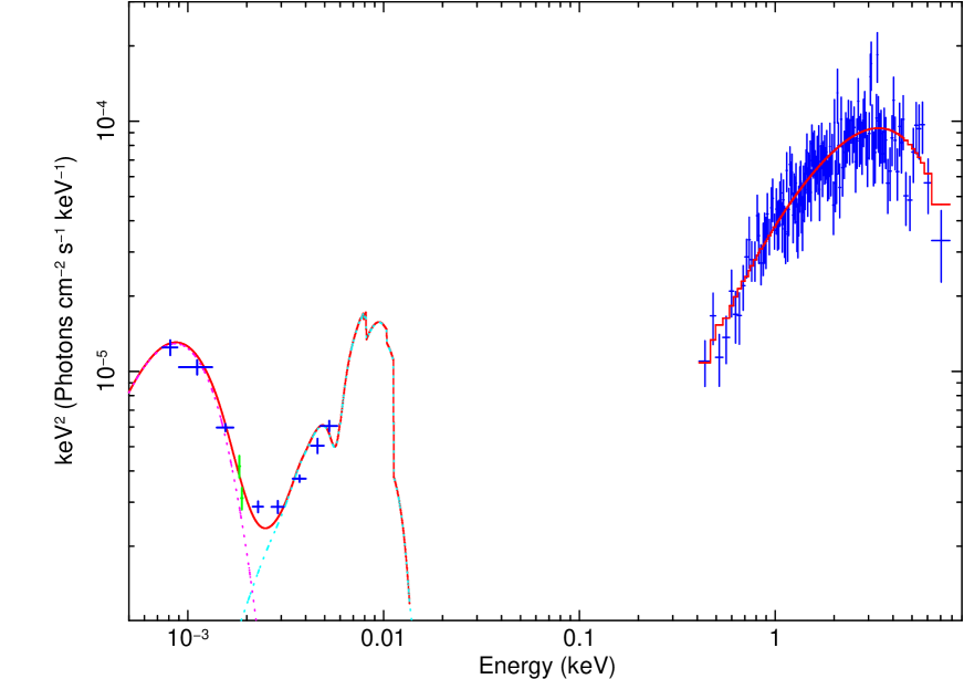
Figure 11: SED plot showing that the optical data require two bb components: one at a characteristic temperature of $\approx(90,000\pm 30,000)$ K and radius $\approx(2.1\pm 0.3)R_{\odot}$ (strongly dependent on the poorly constrained reddening); the other at $T\approx(2700\pm 300)$ K and $R\approx(420\pm 50)R_{\odot}$. Blue datapoints are from Chandra and from broad-band and medium-band filters of HST/WFC3 (Table 3). In addition, we have plotted (green datapoints) the flux density measured in the two narrow-band HST/WFC3 filters with the highest signal to noise ratio (F657N and F673N).

The first hypothesis we tested was that the blue/UV emission may come from the irradiated accretion disk. We re-fitted the combined X-ray spectrum from ObsIDs 2030, 5197 and 22372 with a diskir model in xspec. In the 0.3–8 keV band, diskir is consistent with the fitting results of diskbb discussed earlier (e.g., $kT_{\rm in}\approx 1.3$ keV and $R_{\rm in}\cos\theta\approx 25$ km); however, diskir includes the calculation of the outer disk emission down to the optical/IR band. We found that the observed blue/UV luminosity is $\sim$10% of the soft X-ray luminosity (Figure 11). This fraction is too high to originate from disk reprocessing of X-ray photons according to the diskir model. It would require the disk to intercept $\sim$20% of the X-ray photons (including the albedo term), a level that is not self-consistent with a standard disk model. For plausible reprocessing fractions $\lesssim$0.01, the model irradiated disk contribution to the observed blue/UV emission is $<$10%. The disk contribution to the red/IR emission is much lower, if we assume an outer truncation radius $R_{\rm out}\sim 10^{4}r_{\rm in}$ (a relatively small outer radius is justified by the short binary period, see Section 6.1).

Next, we modelled the near-UV/optical/near-IR emission with a double thermal model (bbodyrad $+$ bbodyrad), in addition to the (small) diskir contribution in xspec. This model includes several free parameters: temperature and radii of the two blackbody components, outer disk radius, reprocessing fraction, intrinsic reddening (which may or may not be the same for the blue and red components). We only have eight broad- or medium-band HST/WFC3 datapoints. Thus, there will inevitably be a degeneracy of acceptable solutions (in particular, reddening and blackbody temperature of the hotter emitter are strongly degenerate). To reduce such degeneracy, we froze the outer disk radius at $R_{\rm out}=10^{4}r_{\rm in}$ and the reprocessing fraction at $f=5\times 10^{-3}$, values that imply a negligible disk contribution to the optical emission.

Our objective here is simply to give an order of magnitude estimate of the size and temperature of the colder and hotter emitter. For low values of the total (intrinsic plus Galactic line-of-sight) reddening $E(B-V)\approx 0.10$ mag (consistent with the X-ray spectral models), we obtained good fits for a blue emitter with a temperature $T_{\rm hot}\approx 60,000$–80,000 K and a radius $R_{\rm hot}\approx(2.0\pm 0.5)R_{\odot}$. For $E(B-V)\approx 0.25$ mag, the preferred temperature range is $T_{\rm hot}\approx 100,000$–120,000 K while the radius is unchanged. Bolometric luminosities of the hotter blackbody component are in the range $\log\left(L_{\rm bol}/L_{\odot}\right)\approx 5.2$–6.0, depending on the choice of reddening. The cooler emitter has acceptable solutions for $T_{\rm cold}\approx 2500$–3000 K, radius $R_{\rm cold}\approx 400$–500 $R_{\odot}$ and bolometric luminosity $\log\left(L_{\rm bol}/L_{\odot}\right)\approx 4.0$.

At a distance modulus of $\approx$27.4 mag, the dereddened absolute brightness of the blue component is $M_{\rm F438W}\approx M_{B}\approx-3.9$ mag to $-3.3$ mag for a range of plausible extinctions. In the $V$ band, the observed flux receives comparable contributions from both the hotter and the cooler emitter (Figure 11). Assuming for example an exact half/half split between the two components, the dereddened $V$-band absolute brightness is $M_{\rm F547M}\approx M_{V}\approx-3.3$ mag to $-2.8$ mag for each of the two components. At longer wavelengths, we estimate a dereddened $I$-band absolute brightness $M_{\rm F814W}\approx M_{I}\approx-5.3$ mag to $-5.0$ mag.

Finally, we measured the brightness in the two narrow-band UVIS filters F657N and F673N. We plotted their flux densities in Figure 11, because they help filling a data gap in the $R$ band, but did not use those two datapoints for our spectral fitting. We do not find evidence for significant brightness at H$\alpha$ and [S II] $\lambda 6716,6731$ in excess of the modelled continuum.

6 Discussion

6.1 Orbital parameters from eclipse duration

For circular orbits, the eclipse fraction $\Delta_{\rm ecl}$ is related to the donor star radius $R_{2}$, the binary separation $a$ and the orbital plane inclination $i$ by the relation

$$\sin i\cos\left(\pi\Delta_{\rm ecl}\right)=\left[1-\left(R_{2}/a\right)^{2}\right]^{1/2}$$ (3)

(Porquet et al., 2005; Chanan et al., 1976). Given the high and persistent (over at least two decades) X-ray luminosity, and the short binary period, we can plausibly assume that the donor star is close to filling its Roche lobe. Thus, applying Eggleton (1983)’s approximation for $R_{2}/a$, we obtain numerical solutions for the mass ratio $q=M_{2}/M_{1}$ as a function of $i$ and $\Delta_{\rm ecl}$:

$$\frac{\ln\left(1+q^{1/3}\right)}{q^{2/3}}=\frac{0.49}{\sqrt{1-\sin^{2}i\cos^{2}\left(\pi\Delta_{\rm ecl}\right)}}-0.60$$ (4)

(Porquet et al., 2005). The minimum value of $q$ corresponds to $i=90^{\circ}$. For the value of $\Delta_{ecl}$ determined for X-1 (Section 3.2), we have $q_{\rm min}=3.0^{+1.7}_{-1.1}$. The importance of this result is that it rules out a low-mass X-ray binary solution for X-1: the donor star must be more massive than the accretor. For a typical NS accretor, the best-fitting estimate suggests $M_{2}\gtrsim 4M_{\odot}$, and for a stellar-mass BH accretor, $M_{2}\gtrsim 15M_{\odot}$.

From the period-density relation

$$P\rho_{2}^{1/2}=0.1375\left(\frac{q}{1+q}\right)^{1/2}\left(R_{2}/a\right)^{-3/2}$$ (5)

(Eggleton, 1983), where $P$ is in days and $\rho_{2}$ is g cm^-3, a mass ratio $q\approx 3$ corresponds to $\rho_{2}\approx 5.9$ g cm^-3. This further rules out main-sequence or giant/supergiant stars, and confirms that the donor star is a stripped star.

6.2 Mass and spectral type of the donor star

We shall assume here for simplicity that $i\approx 90^{\circ}$, and discuss alternative scenarios consistent with $q\approx 3$ inferred from the eclipse duration (Section 6.1), and with the optical brightness derived from the HST images (Section 5). As illustrative examples, for a NS scenario, we take $M_{1}+M_{2}\approx 1.5+4.5=6M_{\odot}$, and for a BH scenario, we assume $M_{1}+M_{2}\approx 7+21=28M_{\odot}$. For the same best-fitting binary period, simple Newtonian physics suggests a binary separation $a\approx 1.5\times 10^{11}$ cm in this NS scenario, with $R_{2}\approx 1.0R_{\odot}$ (Eggleton, 1983); the BH scenario implies $a\approx 2.5\times 10^{11}$ cm, $R_{2}\approx 1.7R_{\odot}$.

Are such values consistent with stellar evolution on the one hand, and with the observed optical brightness on the other? Evolutionary tracks of intermediate-mass stars at Large-Magellanic-Cloud metallicity ($Z=0.006$), stripped of their hydrogen envelope through binary interactions, show (Götberg et al., 2018) that stars with initial masses $M_{\rm i}\approx 18M_{\odot}$ and stripped mass $M\approx 7M_{\odot}$ have effective radius $R_{\rm eff}\approx 1.3R_{\odot}$, effective temperature $T_{\rm eff}\approx 85,000$ K, absolute brightness $M_{B}\approx-2.1$ mag, $M_{V}\approx-1.6$ mag, and bolometric luminosity $\log\left(L_{\rm bol}/L_{\odot}\right)\approx 4.9$. This is still at least 1.2 mag fainter in $B$ and $V$ than the observed blue component, and at least a factor of 3 smaller in $L_{\rm bol}$. Götberg et al. (2018) do not tabulate evolutionary tracks for more massive stripped stars, but, by extrapolating from the trend of their highest-mass tracks, we estimate that stars with $M\gtrsim 10M_{\odot}$ ($M_{\rm i}\gtrsim 25M_{\odot}$) will be consistent with our observed optical brightness and modelled $L_{\rm bol}$.

He stars more massive than $\sim$10 $M_{\odot}$ are generally classified as classical WR stars. Evolutionary tracks (Hamann & Gräfener, 2004; Todt et al., 2015; Gräfener et al., 2017) as well as observations (Hainich et al., 2014, 2015; Hamann et al., 2006) show that only the WN2–WN3 sub-types of WR stars are consistent with the relatively faint $M_{V}\sim-3$ mag inferred for the blue component of the X-1 counterpart. Such early-type nitrogen-sequence WR stars have current masses $\sim$12–16 $M_{\odot}$, bolometric luminosity $\log\left(L_{\rm bol}/L_{\odot}\right)\approx 5.3$–5.6, and $T_{\rm eff}\sim 100,000$–120,000 K.

In summary, comparing the observed optical brightness (with the caveat that a simple blackbody model is only a rough approximation to real stellar spectra) with the predictions from evolutionary tracks, we argue that the blue emitter is most consistent with a He star/WR star with a current mass $10\lesssim\left(M/M_{\odot}\right)\lesssim 16$. Masses near the upper limit of this mass range are required if the accretor is a BH, to explain the long duration of the X-ray eclipse. For a NS accretor, the eclipse duration is consistent with the whole mass range.

Finally, we investigate the origin of the red component (Section 5). At $M_{I}\approx-5$ mag, it is one magnitude brighter than the tip of the red giant branch, but 1–2 magnitudes fainter than typical red supergiants. Instead, it is perfectly consistent with the asymptotic giant branch (AGB) of stars with initial masses $\sim$2–3 $M_{\odot}$, at an age of $\sim$200–1,000 Myr (Padova isochrones: Bressan et al. 2012; Marigo et al. 2013, 2017; Nguyen et al. 2022; see also Cinquegrana et al. 2022). Its temperature $T\approx 2600$–3000 K is consistent with an AGB star but too cold for a red supergiant ($T\sim 3500$–4000 K). Moreover, AGB tracks (especially in their thermally pulsing phases) predict bolometric luminosities $\log\left(L_{\rm bol}/L_{\odot}\right)\approx 4.0$, similar to what we estimated from our blackbody fit.

The presence in the same system of a young He star/WR star (age $\lesssim$20 Myr) and an intermediate-mass AGB star (age $\gtrsim$200 Myr) is baffling. They could not have been formed together. The short binary period required by the X-ray light-curve implies that the 500-$R_{\odot}$ AGB star cannot be the mass donor. Short-period X-ray binaries with persistent $L_{\rm X}\sim L_{\rm Edd}$ are rare and short-lived systems in the local universe (expected lifetime $\lesssim$ few Myr), and thermally pulsing AGB stars are also rare and short-lived (a few Myr). The chance of having an unrelated AGB star spatially aligned (to within $0\farcs{1}$) with the true donor star of X-1 appears low. Thus, it is worth considering alternative scenarios for the two-component optical emission. For example, WR stars produce dust and sometimes show double peaked spectral energy distributions, with a blue and red component (Lau et al., 2019). However, dust sublimates at a temperature of $\approx$1300–2000 K, depending on chemical composition (Phinney, 1989; Kobayashi et al., 2011); this is significantly colder than the red component observed in the HST images. A less implausible scenario is that the red component is a circumbinary (CB) disk or ring, perhaps the remnants of a recently ejected common envelope between the WR star and compact accretor. This scenario is viable if the large CB structure intercepts and re-emits a few per cent of the combined X-ray luminosity from the inner accretion disk and UV luminosity from the WR donor star.

The possibility of a leftover CB disk after common envelope ejection has previously been examined for the case of a white dwarf in the envelope of an AGB star (Kashi & Soker, 2011; De Marco et al., 2011; Passy et al., 2011; Reichardt et al., 2019). In general, for binary systems inside CB disks, tidal transfer of angular momentum from the binary to the disk contributes to a further decrease of the binary separation (Shi et al., 2012; Ma & Li, 2009; Chen & Li, 2006; Artymowicz & Lubow, 1994; Artymowicz et al., 1991), as well as expansion of the CB disk radius (Kashi & Soker, 2011; Chen & Podsiadlowski, 2017). Most of the theoretical work on CB disks has explored the scenario where the inner disk has a net transfer of mass onto the inner binary, in particular onto the less massive of the two components (e.g., Bowen et al., 2018; Farris et al., 2015; Gold et al., 2014; D’Orazio et al., 2013; Shi et al., 2012; Artymowicz & Lubow, 1996). In the case of NGC 4214 X-1, given the expected strong wind mass losses from the WR star, it is more likely that we are in the opposite scenario, of a CB disk being fed (positive mass transfer from the binary to the CB disk) at its inner radius by the binary donor star, and expanding outwards (Dubus et al., 2002). A substantial problem with the CB scenario is how to justify a characteristic size of several 100 $R_{\odot}$ for the optically thick emitter, compared with a binary separation of $\approx$2 $R_{\odot}$. A modelling study of the dynamical stability, accretion rate and size and optical thickness of post-common-envelope CB disks is beyond the scope of this work.

6.3 Reasons for the extended eclipse egress

A distinctive feature of the X-ray eclipses in NGC 4214 X-1, visible in individual cycles (Figure 4) and, more clearly, in the folded light-curve (Figure 5), is the longer duration of egresses compared with ingresses. It takes $\lesssim$1000 s for the flux to drop from peak to minimum value, and, on average, $\approx$4000 s for the flux to recover gradually to peak value after the eclipse. The eclipse profile changes from cycle to cycle, which suggests that it is due to transient and stochastic properties of the medium between the two stars. An egress slower than the ingress is common in the small group of candidate short-period WR systems: Circinus Galaxy X-1 (Qiu et al., 2019), IC 10 X-1 (Laycock et al., 2015a), NGC 300 X-1 (Binder et al., 2011, 2015), NGC 4490 X-1 (Esposito et al., 2013), Cygnus X-3 (Zdziarski et al., 2012; Antokhin et al., 2022). Of those sources, the three systems with the most dramatic eclipse asymmetry and most extended egress duration are also those with the highest luminosity, $L_{\rm X}\gtrsim 10^{39}$ erg s^-1: Circinus Galaxy X-1, NGC 4490 X-1 and NGC 4214 X-1. This asymmetry is not common, instead, in ordinary wind-accreting HMXBs with supergiant donors (Falanga et al., 2015).

We cannot explain the slow egress simply as a gradual decrease of the column density of a cold photo-electric absorber, because of the lack of spectral evolution during egress (Section 4.2). The same lack of spectral evolution is also a distinctive feature of Circinus Galaxy X-1 (Qiu et al., 2019). Our spectral modelling is consistent with either a variable partial covering by opaque clouds, or variable column density of a completely ionized absorber (grey opacity), which may scatter part of the X-ray photons out of our line-of-sight during egress (but not during ingress). The ionization parameter required to explain the observed spectra ($\xi\gtrsim 10^{4}$, Section 4.2) is easily reached in this compact, luminous system, because $\xi\approx 10^{5}L_{39}\,n^{-1}_{12}\,r^{-2}_{11}$ (where $L_{39}\equiv L_{\rm X}/10^{39}$ erg s^-1, $n_{12}\equiv n/10^{12}$ cm^-3, $r_{11}\equiv r/10^{11}$ cm).

The difficulty of the partial covering scenario is that the occulting clouds must be much smaller than the X-ray emitting region (the innermost disk region, within $\lesssim$ a few 100 km), otherwise the X-ray source would only be either fully covered or fully visible. There is no empirical evidence so far for the existence of clumps or winds of that small size. Alternatively, larger, fast-moving clumps may indeed cause the X-ray source to flicker only between fully visible and fully occulted intervals during egress, but on timescales shorter than our time resolution (set by the low observed count rate). If the fraction of fully occulted time within a time resolution element decreases, the process appears to us as a “gradual” flux recovery. This scenario would be empirically indistinguishable from the partial covering scenario.

The reason for the apparently grey opacity and the reason for the asymmetric distribution of the absorber in ingress and egress are likely to be physically connected. The observed asymmetry implies that the additional absorber must be either leading the compact object or trailing the donor star. The former scenario could be explained as a bow shock, caused by the supersonic orbital motion of the compact object inside the WR wind (Hunt, 1971; Theuns & Jorissen, 1993; Wang & Loeb, 2014). This is the scenario invoked by Qiu et al. (2019) for Circinus Galaxy X-1 and by Antokhin et al. (2022) for Cyg X-3. The latter scenario relies on the presence of a “shadow wind” in the system (Blondin 1994 and Blondin & Woo 1995 for hydrodynamical simulations; Laycock et al. 2015b for an application of this scenario to the WR system IC 10 X-1). In a compact, luminous system, the X-ray photons from the compact object suppress or strongly decrease the radiatively driven wind from the donor star, except from its shaded side (Blondin, 1994; Vilhu et al., 2021). Coriolis forces deflect the shadow wind towards the trailing side of the donor star: this is the reason why it appears between us and the compact object in eclipse egress but not in ingress. As the wind leaves the WR shadow, it stalls and gets highly ionized (Blondin, 1994). In our grey opacity scenario, this is the ionized medium responsible for scattering some of the X-ray photons out of our line of sight. Further analysis of the integrated column density of the shadow wind is beyond the scope of this work.

7 Conclusions

We combined new and archival Chandra and HST data for a study of the short-period, eclipsing X-ray binary NGC 4214 X-1. We confirmed that the source is still active and still showing eclipses, with an out-of-eclipse luminosity $L_{\rm X}\approx 10^{39}$ erg s^-1, 19 years after the first Chandra observation. Persistently active sources at such high luminosities tend to have high-mass donors, although here we do not have direct information (such as radial velocity curves) to constrain the mass of the donor star. We refined the estimate of the orbital period, $P\approx(12940\pm 270)$ s, and the average eclipse duration, $\Delta T_{\rm ecl}\approx(2050\pm 175)$ s. From the high eclipse fraction, $\Delta_{\rm ecl}\approx 0.16$, we derive a minimum mass ratio $q_{\rm min}>2$ (and, most likely, $q\gtrsim 3$), which again suggests that the system is an HXMB. At the same time, the short binary period rules out main sequence or supergiant donors, and is only consistent with a WR star or an intermediate-mass stripped He star.

From the HST/WFC3 observations, we discovered the likely optical counterpart, at an apparent brightness $V\approx 24$ mag and an absolute magnitude $M_{V}\approx-3$ mag, $M_{I}\approx-5$ mag. The optical source is inconsistent with a single thermal component, and consists instead of two clearly distinct components: a blue one, with $T_{\rm hot}\gtrsim 60,000$ K and characteristic radius $R_{\rm hot}\approx 2R_{\odot}$, and a red one, with $T_{\rm cold}\approx 2,700$ K and characteristic radius $R_{\rm hot}\approx 400R_{\odot}$. The blue emission is consistent with a WR star, in particular from the compact, early-type WN class, with stripped mass $\sim$12–16 $M_{\odot}$. The red component is either an unrelated AGB star from an older stellar population, projected on the sky at the same location as the true optical counterpart (within $0\farcs{1}$), or it is emission from a CB disk, perhaps fed by the WR wind.

Our X-ray timing and spectral study highlights two properties that seem to characterize the rare class of luminous (near- or super-Eddington) WR HMXBs: i) a highly asymmetric eclipse profile, with a sharp ingress and a longer egress; ii) a lack of spectral evolution during the slow egress, as the observed flux increases. The asymmetry suggests that most of the absorbing material is either leading the compact object, or trailing the donor star, along their orbital motion. We speculate that, in the first scenario, the absorbing material could be associated with a bow shock in front of the compact object; in the latter scenario, it could be the shadow wind from the un-irradiated face of the donor star, which is launched in the radial direction but trails the star because of its orbital motion. The strong X-ray luminosity and small binary separation ensure that as soon as this wind component leaves the shadow region, it gets completely ionized ($\xi\gtrsim 10,000$). This would explain why its effect on the observed X-ray spectrum is via Thomson scattering of photons out of our line of sight (grey opacity) rather than photo-electric absorption.

We cannot rule out either a NS or a BH nature of the compact object. However, a near-Eddington BH interpretation appears more consistent with the observed X-ray spectrum, which is well modelled by a disk-blackbody with $kT_{\rm in}\approx 1.3$ keV and $R_{\rm{in}}\sqrt{\cos\theta}\approx 25$ km. A BH nature of the compact object would also be consistent with the suggestion that BHs are more likely to survive a common envelope phase, prelude to the formation of short-period WR X-ray binaries (van den Heuvel et al., 2017). In any case, NGC 4214 X-1 will eventually produce a double compact object binaries, tight enough to merge via gravitational wave emission on timescales of a few $10^{7}$ yr. Only a handful of such systems have been detected so far, partly because of observation biases: that is, we may not recognize similar systems (bright HMXBs) when they are seen more face-on, without observable X-ray eclipses.

Appendix A X-ray properties of SNRs in NGC 4214

As a serendipitous result, we searched for X-ray counterparts of the seven SNRs identified by Dopita et al. (2010) in this galaxy. Six of them (all except the 4th one in their list) are recovered in the combined Chandra image (Figure 1), which has a total exposure of 141 ks. We assumed that the luminosity of the SNRs remained constant across the four Chandra observations, and that their spectra could be approximated with a thermal plasma model (apec model in xspec) at $kT\approx 0.5$ keV. We fitted the spectra of two SNRs (SNR2 and SNR5) with high signal-to-noise ratio and relatively low contamination from diffuse hot gas emission, and provided a rough estimate of the luminosities of the other four SNRs based on their scaled count rates (Table 7). We find five SNRs with luminosities $>$10³⁶ erg s^-1, up to a maximum luminosity $\approx 3\times 10^{36}$ erg s^-1. Taking into account the small number statistics, this is perfectly consistent with the expected number and luminosities of such sources, by comparison with the high-end of the X-ray SNR luminosity functions seen in the LMC (Maggi et al., 2016) and in M 33 (Garofali et al., 2017), which have star formation rates $\approx$3–4 times higher than NGC 4214 (Harris & Zaritsky, 2009; Antoniou & Zezas, 2016; Williams et al., 2013).

Table 7: X-ray properties of the optically identified SNRs (Dopita et al., 2010) recovered in the Chandra observations of NGC 4214.

Source	RA	DEC	Net Rate	0.3–7 keV Flux	0.3–10 keV Luminosity
	(hms)	(hms)	($10^{-5}$ ct/s)	($10^{-15}$ erg cm-2 s-1)	($10^{36}$ erg s-1)
SNR1	12:15:38.963	+36:18:58.85	$9.0\pm 3.1$	$0.5\pm 0.2$	$0.8\pm 0.3$
SNR2	12:15:40.000	+36:18:40.72	$36.5\pm 5.6$	$2.1\pm 0.3$	$3.1\pm 0.4$
SNR3	12:15:40.008	+36:19:36.00	$34.7\pm 7.0$	$2.1\pm 0.4$	$3.1\pm 0.5$
SNR5	12:15:41.136	+36:19:15.04	$21.1\pm 4.4$	$1.1\pm 0.2$	$1.4\pm 0.3$
SNR6	12:15:42.456	+36:19:47.78	$14.5\pm 4.0$	$0.8\pm 0.2$	$1.2\pm 0.3$
SNR7	12:15:45.639	+36:19:41.50	$19.6\pm 4.4$	$1.0\pm 0.2$	$1.3\pm 0.3$

References

- Abe et al. (2005) Abe, Y., Fukazawa, Y., Kubota, A., Kasama, D., & Makishima, K. 2005, PASJ, 57, 629, doi: 10.1093/pasj/57.4.629
- Antokhin et al. (2022) Antokhin, I. I., Cherepashchuk, A. M., Antokhina, E. A., & Tatarnikov, A. M. 2022, ApJ, 926, 123, doi: 10.3847/1538-4357/ac4047
- Antoniou & Zezas (2016) Antoniou, V., & Zezas, A. 2016, MNRAS, 459, 528, doi: 10.1093/mnras/stw167
- Arnaud (1996) Arnaud, K. A. 1996, in Astronomical Society of the Pacific Conference Series, Vol. 101, Astronomical Data Analysis Software and Systems V, ed. G. H. Jacoby & J. Barnes, 17
- Artymowicz et al. (1991) Artymowicz, P., Clarke, C. J., Lubow, S. H., & Pringle, J. E. 1991, ApJ, 370, L35, doi: 10.1086/185971
- Artymowicz & Lubow (1994) Artymowicz, P., & Lubow, S. H. 1994, ApJ, 421, 651, doi: 10.1086/173679
- Artymowicz & Lubow (1996) —. 1996, ApJ, 467, L77, doi: 10.1086/310200
- Barnard et al. (2008) Barnard, R., Clark, J. S., & Kolb, U. C. 2008, A&A, 488, 697, doi: 10.1051/0004-6361:20077975
- Belczynski et al. (2013) Belczynski, K., Bulik, T., Mandel, I., et al. 2013, ApJ, 764, 96, doi: 10.1088/0004-637X/764/1/96
- Belczynski et al. (2016) Belczynski, K., Holz, D. E., Bulik, T., & O’Shaughnessy, R. 2016, Nature, 534, 512, doi: 10.1038/nature18322
- Bhattacharya et al. (2023) Bhattacharya, S., Laycock, S. G. T., Chené, A.-N., et al. 2023, ApJ, 944, 52, doi: 10.3847/1538-4357/acb155
- Binder et al. (2011) Binder, B., Williams, B. F., Eracleous, M., et al. 2011, ApJ, 742, 128, doi: 10.1088/0004-637X/742/2/128
- Binder et al. (2015) —. 2015, AJ, 150, 94, doi: 10.1088/0004-6256/150/3/94
- Binder et al. (2021) Binder, B. A., Sy, J. M., Eracleous, M., et al. 2021, ApJ, 910, 74, doi: 10.3847/1538-4357/abe6a9
- Blackburn (1995) Blackburn, J. K. 1995, in Astronomical Society of the Pacific Conference Series, Vol. 77, Astronomical Data Analysis Software and Systems IV, ed. R. A. Shaw, H. E. Payne, & J. J. E. Hayes, 367
- Blondin (1994) Blondin, J. M. 1994, ApJ, 435, 756, doi: 10.1086/174853
- Blondin & Woo (1995) Blondin, J. M., & Woo, J. W. 1995, ApJ, 445, 889, doi: 10.1086/175748
- Bowen et al. (2018) Bowen, D. B., Mewes, V., Campanelli, M., et al. 2018, ApJ, 853, L17, doi: 10.3847/2041-8213/aaa756
- Bressan et al. (2012) Bressan, A., Marigo, P., Girardi, L., et al. 2012, MNRAS, 427, 127, doi: 10.1111/j.1365-2966.2012.21948.x
- Carpano et al. (2007) Carpano, S., Pollock, A. M. T., Prestwich, A., et al. 2007, A&A, 466, L17, doi: 10.1051/0004-6361:20077363
- Cash (1979) Cash, W. 1979, ApJ, 228, 939, doi: 10.1086/156922
- Chanan et al. (1976) Chanan, G. A., Middleditch, J., & Nelson, J. E. 1976, ApJ, 208, 512, doi: 10.1086/154633
- Chen & Li (2006) Chen, W.-C., & Li, X.-D. 2006, MNRAS, 373, 305, doi: 10.1111/j.1365-2966.2006.11032.x
- Chen & Podsiadlowski (2017) Chen, W.-C., & Podsiadlowski, P. 2017, ApJ, 837, L19, doi: 10.3847/2041-8213/aa624a
- Choi et al. (2020) Choi, Y., Dalcanton, J. J., Williams, B. F., et al. 2020, ApJ, 902, 54, doi: 10.3847/1538-4357/abb467
- Cinquegrana et al. (2022) Cinquegrana, G. C., Joyce, M., & Karakas, A. I. 2022, ApJ, 939, 50, doi: 10.3847/1538-4357/ac87ae
- Crowther et al. (2010) Crowther, P. A., Barnard, R., Carpano, S., et al. 2010, MNRAS, 403, L41, doi: 10.1111/j.1745-3933.2010.00811.x
- Dalcanton et al. (2009) Dalcanton, J. J., Williams, B. F., Seth, A. C., et al. 2009, ApJS, 183, 67, doi: 10.1088/0067-0049/183/1/67
- De Marco et al. (2011) De Marco, O., Passy, J.-C., Moe, M., et al. 2011, MNRAS, 411, 2277, doi: 10.1111/j.1365-2966.2010.17891.x
- Dopita et al. (2010) Dopita, M. A., Calzetti, D., Maíz Apellániz, J., et al. 2010, Ap&SS, 330, 123, doi: 10.1007/s10509-010-0376-0
- D’Orazio et al. (2013) D’Orazio, D. J., Haiman, Z., & MacFadyen, A. 2013, MNRAS, 436, 2997, doi: 10.1093/mnras/stt1787
- Dubus et al. (2002) Dubus, G., Taam, R. E., & Spruit, H. C. 2002, ApJ, 569, 395, doi: 10.1086/339266
- Eggleton (1983) Eggleton, P. P. 1983, ApJ, 268, 368, doi: 10.1086/160960
- Esposito et al. (2015) Esposito, P., Israel, G. L., Milisavljevic, D., et al. 2015, MNRAS, 452, 1112, doi: 10.1093/mnras/stv1379
- Esposito et al. (2013) Esposito, P., Israel, G. L., Sidoli, L., et al. 2013, MNRAS, 436, 3380, doi: 10.1093/mnras/stt1819
- Falanga et al. (2015) Falanga, M., Bozzo, E., Lutovinov, A., et al. 2015, A&A, 577, A130, doi: 10.1051/0004-6361/201425191
- Farris et al. (2015) Farris, B. D., Duffell, P., MacFadyen, A. I., & Haiman, Z. 2015, MNRAS, 447, L80, doi: 10.1093/mnrasl/slu184
- Fruscione et al. (2006) Fruscione, A., McDowell, J. C., Allen, G. E., et al. 2006, in Society of Photo-Optical Instrumentation Engineers (SPIE) Conference Series, Vol. 6270, Society of Photo-Optical Instrumentation Engineers (SPIE) Conference Series, ed. D. R. Silva & R. E. Doxsey, 62701V, doi: 10.1117/12.671760
- Garofali et al. (2017) Garofali, K., Williams, B. F., Plucinsky, P. P., et al. 2017, MNRAS, 472, 308, doi: 10.1093/mnras/stx1905
- Ghosh et al. (2006) Ghosh, K. K., Rappaport, S., Tennant, A. F., et al. 2006, ApJ, 650, 872, doi: 10.1086/507124
- Gold et al. (2014) Gold, R., Paschalidis, V., Etienne, Z. B., Shapiro, S. L., & Pfeiffer, H. P. 2014, Phys. Rev. D, 89, 064060, doi: 10.1103/PhysRevD.89.064060
- Götberg et al. (2018) Götberg, Y., de Mink, S. E., Groh, J. H., et al. 2018, A&A, 615, A78, doi: 10.1051/0004-6361/201732274
- Gräfener et al. (2017) Gräfener, G., Owocki, S. P., Grassitelli, L., & Langer, N. 2017, A&A, 608, A34, doi: 10.1051/0004-6361/201731590
- Hainich et al. (2015) Hainich, R., Pasemann, D., Todt, H., et al. 2015, A&A, 581, A21, doi: 10.1051/0004-6361/201526241
- Hainich et al. (2014) Hainich, R., Rühling, U., Todt, H., et al. 2014, A&A, 565, A27, doi: 10.1051/0004-6361/201322696
- Hamann & Gräfener (2004) Hamann, W. R., & Gräfener, G. 2004, A&A, 427, 697, doi: 10.1051/0004-6361:20040506
- Hamann et al. (2006) Hamann, W. R., Gräfener, G., & Liermann, A. 2006, A&A, 457, 1015, doi: 10.1051/0004-6361:20065052
- Harris & Zaritsky (2009) Harris, J., & Zaritsky, D. 2009, AJ, 138, 1243, doi: 10.1088/0004-6256/138/5/1243
- Hartwell et al. (2004) Hartwell, J. M., Stevens, I. R., Strickland, D. K., Heckman, T. M., & Summers, L. K. 2004, MNRAS, 348, 406, doi: 10.1111/j.1365-2966.2004.07375.x
- HI4PI Collaboration et al. (2016) HI4PI Collaboration, Ben Bekhti, N., Flöer, L., et al. 2016, A&A, 594, A116, doi: 10.1051/0004-6361/201629178
- Hjalmarsdotter et al. (2009) Hjalmarsdotter, L., Zdziarski, A. A., Szostek, A., & Hannikainen, D. C. 2009, MNRAS, 392, 251, doi: 10.1111/j.1365-2966.2008.14036.x
- Hunt (1971) Hunt, R. 1971, MNRAS, 154, 141, doi: 10.1093/mnras/154.2.141
- Kashi & Soker (2011) Kashi, A., & Soker, N. 2011, MNRAS, 417, 1466, doi: 10.1111/j.1365-2966.2011.19361.x
- Kobayashi et al. (2011) Kobayashi, H., Kimura, H., Watanabe, S. i., Yamamoto, T., & Müller, S. 2011, Earth, Planets and Space, 63, 1067, doi: 10.5047/eps.2011.03.012
- Kobulnicky & Skillman (1996) Kobulnicky, H. A., & Skillman, E. D. 1996, ApJ, 471, 211, doi: 10.1086/177964
- Koljonen et al. (2010) Koljonen, K. I. I., Hannikainen, D. C., McCollough, M. L., Pooley, G. G., & Trushkin, S. A. 2010, MNRAS, 406, 307, doi: 10.1111/j.1365-2966.2010.16722.x
- Kretschmar et al. (2019) Kretschmar, P., Fürst, F., Sidoli, L., et al. 2019, New A Rev., 86, 101546, doi: 10.1016/j.newar.2020.101546
- Kubota & Makishima (2004) Kubota, A., & Makishima, K. 2004, ApJ, 601, 428, doi: 10.1086/380433
- Kubota et al. (1998) Kubota, A., Tanaka, Y., Makishima, K., et al. 1998, PASJ, 50, 667, doi: 10.1093/pasj/50.6.667
- Lau et al. (2019) Lau, R. M., Heida, M., Walton, D. J., et al. 2019, ApJ, 878, 71, doi: 10.3847/1538-4357/ab1b1c
- Laycock et al. (2015a) Laycock, S. G. T., Cappallo, R. C., & Moro, M. J. 2015a, MNRAS, 446, 1399, doi: 10.1093/mnras/stu2151
- Laycock et al. (2015b) Laycock, S. G. T., Maccarone, T. J., & Christodoulou, D. M. 2015b, MNRAS, 452, L31, doi: 10.1093/mnrasl/slv082
- Lommen et al. (2005) Lommen, D., Yungelson, L., van den Heuvel, E., Nelemans, G., & Portegies Zwart, S. 2005, A&A, 443, 231, doi: 10.1051/0004-6361:20052824
- Ma & Li (2009) Ma, B., & Li, X.-D. 2009, ApJ, 698, 1907, doi: 10.1088/0004-637X/698/2/1907
- Maccarone et al. (2014) Maccarone, T. J., Lehmer, B. D., Leyder, J. C., et al. 2014, MNRAS, 439, 3064, doi: 10.1093/mnras/stu167
- MacKenty et al. (2000) MacKenty, J. W., Maíz-Apellániz, J., Pickens, C. E., Norman, C. A., & Walborn, N. R. 2000, AJ, 120, 3007, doi: 10.1086/316841
- Maggi et al. (2016) Maggi, P., Haberl, F., Kavanagh, P. J., et al. 2016, A&A, 585, A162, doi: 10.1051/0004-6361/201526932
- Makishima et al. (1986) Makishima, K., Maejima, Y., Mitsuda, K., et al. 1986, ApJ, 308, 635, doi: 10.1086/164534
- Mandel & Broekgaarden (2022) Mandel, I., & Broekgaarden, F. S. 2022, Living Reviews in Relativity, 25, 1, doi: 10.1007/s41114-021-00034-3
- Marchant et al. (2017) Marchant, P., Langer, N., Podsiadlowski, P., et al. 2017, A&A, 604, A55, doi: 10.1051/0004-6361/201630188
- Marigo et al. (2013) Marigo, P., Bressan, A., Nanni, A., Girardi, L., & Pumo, M. L. 2013, MNRAS, 434, 488, doi: 10.1093/mnras/stt1034
- Marigo et al. (2017) Marigo, P., Girardi, L., Bressan, A., et al. 2017, ApJ, 835, 77, doi: 10.3847/1538-4357/835/1/77
- Mason et al. (1985) Mason, K. O., Parmar, A. N., & White, N. E. 1985, MNRAS, 216, 1033, doi: 10.1093/mnras/216.4.1033
- McClintock et al. (2014) McClintock, J. E., Narayan, R., & Steiner, J. F. 2014, Space Sci. Rev., 183, 295, doi: 10.1007/s11214-013-0003-9
- McCollough et al. (2016) McCollough, M. L., Corrales, L., & Dunham, M. M. 2016, ApJ, 830, L36, doi: 10.3847/2041-8205/830/2/L36
- McQuinn et al. (2010) McQuinn, K. B. W., Skillman, E. D., Cannon, J. M., et al. 2010, ApJ, 721, 297, doi: 10.1088/0004-637X/721/1/297
- Nasa High Energy Astrophysics Science Archive Research Center (2014) (Heasarc) Nasa High Energy Astrophysics Science Archive Research Center (Heasarc). 2014, HEAsoft: Unified Release of FTOOLS and XANADU, Astrophysics Source Code Library, record ascl:1408.004. http://ascl.net/1408.004
- Nguyen et al. (2022) Nguyen, C. T., Costa, G., Girardi, L., et al. 2022, A&A, 665, A126, doi: 10.1051/0004-6361/202244166
- Passy et al. (2011) Passy, J. C., De Marco, O., Fryer, C. L., et al. 2011, in Astronomical Society of the Pacific Conference Series, Vol. 447, Evolution of Compact Binaries, ed. L. Schmidtobreick, M. R. Schreiber, & C. Tappert, 107
- Phinney (1989) Phinney, E. S. 1989, in NATO Advanced Study Institute (ASI) Series C, Vol. 290, Theory of Accretion Disks, ed. F. Meyer, 457
- Porquet et al. (2005) Porquet, D., Grosso, N., Bélanger, G., et al. 2005, A&A, 443, 571, doi: 10.1051/0004-6361:20053214
- Prestwich et al. (2007) Prestwich, A. H., Kilgard, R., Crowther, P. A., et al. 2007, ApJ, 669, L21, doi: 10.1086/523755
- Qiu & Soria (2019) Qiu, Y., & Soria, R. 2019, IAU Symposium, 346, 228, doi: 10.1017/S1743921318007482
- Qiu et al. (2019) Qiu, Y., Soria, R., Wang, S., et al. 2019, ApJ, 877, 57, doi: 10.3847/1538-4357/ab16e7
- Reichardt et al. (2019) Reichardt, T. A., De Marco, O., Iaconi, R., Tout, C. A., & Price, D. J. 2019, MNRAS, 484, 631, doi: 10.1093/mnras/sty3485
- Remillard & McClintock (2006) Remillard, R. A., & McClintock, J. E. 2006, ARA&A, 44, 49, doi: 10.1146/annurev.astro.44.051905.092532
- Sander & Vink (2020) Sander, A. A. C., & Vink, J. S. 2020, MNRAS, 499, 873, doi: 10.1093/mnras/staa2712
- Sander et al. (2020) Sander, A. A. C., Vink, J. S., & Hamann, W. R. 2020, MNRAS, 491, 4406, doi: 10.1093/mnras/stz3064
- Shi et al. (2012) Shi, J.-M., Krolik, J. H., Lubow, S. H., & Hawley, J. F. 2012, ApJ, 749, 118, doi: 10.1088/0004-637X/749/2/118
- Silverman & Filippenko (2008) Silverman, J. M., & Filippenko, A. V. 2008, ApJ, 678, L17, doi: 10.1086/588096
- Steiner et al. (2016) Steiner, J. F., Walton, D. J., García, J. A., et al. 2016, ApJ, 817, 154, doi: 10.3847/0004-637X/817/2/154
- Sutton et al. (2017) Sutton, A. D., Swartz, D. A., Roberts, T. P., et al. 2017, ApJ, 836, 48, doi: 10.3847/1538-4357/836/1/48
- Szostek et al. (2008) Szostek, A., Zdziarski, A. A., & McCollough, M. L. 2008, MNRAS, 388, 1001, doi: 10.1111/j.1365-2966.2008.13479.x
- Theuns & Jorissen (1993) Theuns, T., & Jorissen, A. 1993, MNRAS, 265, 946, doi: 10.1093/mnras/265.4.946
- Todt et al. (2015) Todt, H., Sander, A., Hainich, R., et al. 2015, A&A, 579, A75, doi: 10.1051/0004-6361/201526253
- Úbeda et al. (2007) Úbeda, L., Maíz-Apellániz, J., & MacKenty, J. W. 2007, AJ, 133, 932, doi: 10.1086/509503
- van den Heuvel (2019) van den Heuvel, E. P. J. 2019, IAU Symposium, 346, 1, doi: 10.1017/S1743921319001315
- van den Heuvel & De Loore (1973) van den Heuvel, E. P. J., & De Loore, C. 1973, A&A, 25, 387
- van den Heuvel et al. (2017) van den Heuvel, E. P. J., Portegies Zwart, S. F., & de Mink, S. E. 2017, MNRAS, 471, 4256, doi: 10.1093/mnras/stx1430
- Veledina et al. (2023) Veledina, A., Muleri, F., Poutanen, J., et al. 2023, arXiv e-prints, arXiv:2303.01174, doi: 10.48550/arXiv.2303.01174
- Vilhu et al. (2021) Vilhu, O., Kallman, T. R., Koljonen, K. I. I., & Hannikainen, D. C. 2021, A&A, 649, A176, doi: 10.1051/0004-6361/202140620
- Walter et al. (2015) Walter, R., Lutovinov, A. A., Bozzo, E., & Tsygankov, S. S. 2015, A&A Rev., 23, 2, doi: 10.1007/s00159-015-0082-6
- Wang & Loeb (2014) Wang, X., & Loeb, A. 2014, MNRAS, 441, 809, doi: 10.1093/mnras/stu600
- Weisskopf et al. (2004) Weisskopf, M. C., Wu, K., Tennant, A. F., Swartz, D. A., & Ghosh, K. K. 2004, ApJ, 605, 360, doi: 10.1086/381307
- Williams et al. (2011) Williams, B. F., Dalcanton, J. J., Gilbert, K. M., et al. 2011, ApJ, 735, 22, doi: 10.1088/0004-637X/735/1/22
- Williams et al. (2013) Williams, B. F., Dalcanton, J. J., Stilp, A., et al. 2013, ApJ, 765, 120, doi: 10.1088/0004-637X/765/2/120
- Zdziarski et al. (2013) Zdziarski, A. A., Mikolajewska, J., & Belczynski, K. 2013, MNRAS, 429, L104, doi: 10.1093/mnrasl/sls035
- Zdziarski et al. (2012) Zdziarski, A. A., Sikora, M., Dubus, G., et al. 2012, MNRAS, 421, 2956, doi: 10.1111/j.1365-2966.2012.20519.x