Exact solution of the infinite-range dissipative transverse-field Ising model

Abstract

The dissipative variant of the Ising model in a transverse field is one of the most important models in the analysis of open quantum many-body systems, due to its paradigmatic character for understanding driven-dissipative quantum phase transitions, as well as its relevance in modelling diverse experimental platforms in atomic physics and quantum simulation. Here, we present an exact solution for the steady state of the transverse-field Ising model in the limit of infinite-range interactions, with local dissipation and inhomogeneous transverse fields. Our solution holds despite the lack of any collective spin symmetry or even permutation symmetry. It allows us to investigate first- and second-order dissipative phase transitions, driven-dissipative criticality, and captures the emergence of a surprising “spin blockade” phenomenon. The ability of the solution to describe spatially-varying local fields provides a new tool to study disordered open quantum systems in regimes that would be extremely difficult to treat with numerical methods.

Introduction. Dissipative transverse-field Ising (DTI) models are a paradigmatic class of open quantum systems in atomic physics, quantum information and quantum simulation. In these systems, a collection of spins interact on a lattice via Ising interactions, while subject to local magnetic fields that are transverse to the interaction axis; these fields can represent local Rabi drives in a rotating frame. Markovian dissipation is most commonly introduced via Lindblad dynamics with jump operators that induce either local dephasing Marcuzzi et al. (2014); Borish et al. (2020) or local $T_{1}$ relaxation Bloch (1946) along chosen axes Jin et al. (2018); Lee et al. (2012); Kazemi and Weimer (2023); Singh and Weimer (2022); Weimer (2015); Overbeck et al. (2017). Interest in this model stems from its direct relevance in understanding diverse experimental platforms ranging across atomic physics. In dilute Rydberg gases, the mean-field equations of the DTI have been used to qualitatively capture bistability and hysteresis in the magnetization density when sweeping laser detunings Carr et al. (2013); Malossi et al. (2014); Paris-Mandoki et al. (2017). In quantum simulation platforms such as trapped ions, the DTI model has been realized with tunable power-law decaying interactions $J_{ij}=J_{0}/|i-j|^{\alpha}$ that approach the infinite-range limit with $0<\alpha<3$ Britton et al. (2012). More recently, arrays of Rydberg atoms, with much shorter-range and stronger Ising interactions, have emerged as a versatile platform for simulating many-body quantum systems, and have realized the DTI on, e.g. triangular and hypercubic lattices Ebadi et al. (2021); Scholl et al. (2021).

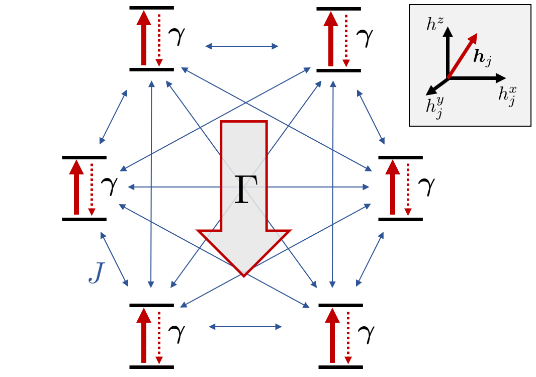
Figure 1: Schematic of our solvable dissipative transverse-field Ising model. A collection of $N$ spin-1/2 particles, represented here as a collection of driven-dissipative two-level systems, is subject to local $T_{1}$ decay at a rate $\gamma$, as well as collective decay at a rate $\Gamma$. The two-level systems interact via an all-to-all Ising interaction with strength $J$. Inset: each spin is subject to a separate external magnetic field with both axial and transverse components. The axial component of the external field is the same for each spin, whereas the transverse part can vary.

Solutions for the DTI nonequilibrium steady state have been lacking, mainly due to the difficulty in understanding the competition between the transverse field and the dissipation. Without a transverse field, the Lindblad dynamics is integrable due to the existence of a complete set of commuting weak symmetries Foss-Feig et al. (2013); McDonald and Clerk (2022), and the steady-state problem is essentially a classical one. However, when the transverse field is present, even in the simplest case $\alpha=0$, an analytical solution that is valid in all parameter regimes is still lacking. In this Letter, we address this issue by finding a “hidden” symmetry Roberts et al. (2021); Fagnola and Umanità (2010) in the dynamics of the DTI model, leading to an exact solution for its dissipative steady state in the infinite-range limit. Our analytical solution remains valid for systems with inhomogeneous transverse fields, where the dynamics is not simplified by permutation symmetry.

Equipped with the exact solution, we are able to derive closed-form expressions for correlation functions of any order, offering valuable insights into the system’s behavior. We also investigate a novel spin blockade effect characterized by unconventional correlation properties, and uncover an effective “thermodynamic potential” which allows us to fully understand the large-$N$ limit, and which incorporates non-mean-field information, including the location of first-order phase transitions in regimes far from the critical point Marcuzzi et al. (2014); Paz and Maghrebi (2021).

Dissipative transverse-field Ising model. We consider a dissipative system consisting of spin-$1/2$ particles described by the local spin observables $\hat{S}^{\mu}_{j}=\hat{\sigma}^{\mu}_{j}/2$, with $\mu=x,y,z$ denoting the spin direction and $j=1,2,\dots,N$ indexing the lattice sites. Here, $\hat{\sigma}^{\mu}_{j}$ denote the Pauli matrices. The spins are coupled via an all-to-all Ising interaction, and we allow for each lattice site to experience a different magnetic field $h_{j}^{\mu}$, which can have both transverse and axial components:

$$\hat{H}_{\text{TFIM}}=J\sum_{i\neq j}\hat{S}^{z}_{i}\hat{S}^{z}_{j}+\sum_{j,\mu}h^{\mu}_{j}\hat{S}^{\mu}_{j}$$ (1)

This Hamiltonian can be viewed as representing a collection of Rabi-driven two-level systems in the rotating frame, with the transverse- and axial fields corresponding to the drive amplitude and detuning of each local two-level system.

The full dynamics of our solvable model Singh and Weimer (2022); Huybrechts et al. (2020a) also includes both collective and local $T_{1}$ decay for each two-level system and is described by the Lindblad master equation

$$\displaystyle{\dot{\hat{\rho}}=-i[\hat{H}_{\text{TFIM}},\hat{\rho}]+\gamma\sum_{j}\mathcal{D}[\hat{\sigma}^{-}_{j}]\hat{\rho}+\Gamma\mathcal{D}[\hat{S}_{-}]\hat{\rho}}\equiv\mathcal{L}\hat{\rho},$$ (2)

where $\mathcal{D}[\hat{X}]\hat{\rho}\equiv\hat{X}\hat{\rho}\hat{X}^{\dagger}-(1/2)\{\hat{X}^{\dagger}\hat{X},\hat{\rho}\}$ is the usual Lindblad dissipative superoperator, $\gamma\equiv 1/T_{1}$ is the local longitudinal relaxation rate, and $\Gamma$ is a rate for collective relaxation that is relevant in many platforms, capturing effects such as superradiant decay Carr et al. (2013). Finally, $\hat{S}_{-}:=\hat{S}^{x}-i\hat{S}^{y}$ is the lowering operator for the collective $SU(2)$ representation $\hat{S}^{\mu}:=\sum_{j}\hat{S}^{\mu}_{j}$. Throughout the rest of this Letter, we will fix the axial component of the magnetic field to be spatially uniform ($h^{z}_{j}\equiv h^{z}$), and will (without loss of any generality) set $h^{y}_{j}=0$.

We focus exclusively on finding the steady states of this system, i.e. density matrices $\hat{\rho}_{\text{SS}}$ satisfying

$$\mathcal{L}\hat{\rho}_{\text{SS}}=0.$$ (3)

We briefly summarize prior work on this model. Even in the case that the external field $h^{\mu}_{j}$ is uniform, there has been no known exact solution for its steady state, although there has been much work studying asymptotic expansions in the semiclassical limit $N\to\infty$ Lee et al. (2012); Lee and Chan (2013); Ates et al. (2012); Weimer (2015); Paz and Maghrebi (2021). Mean-field approximations for the steady states satisfying Eq. (3) have been used to qualitatively model dissipative phase transitions in dilute Rydberg gases trapped in, e.g. vapor cells Carr et al. (2013); Malossi et al. (2014); Marcuzzi et al. (2014), and have been proven to be exact in the limit $N\to\infty$ Carollo and Lesanovsky (2021); Fiorelli et al. (2023). For $N$ finite, the dissipative steady state has been studied using numerical methods that take advantage of the permutation symmetry of the problem Huybrechts et al. (2020b); Jo et al. (2022).

Exact steady-state solution. Suppose that $\mathcal{L}$ were the Liouvillian for a classical master equation. In this case, a common method for solving Eq. (3) would be to impose detailed balance conditions on the steady-state probability density Kelley (1979). In our case, we factor the steady state into two pieces, $\hat{\rho}_{\text{SS}}=\hat{\Psi}\hat{\Psi}^{\dagger}$, with $\hat{\Psi}$ antilinear, and impose the quantum detailed balance conditions Fagnola and Umanita (2007); Fagnola and Umanità (2010)

$$\hat{H}_{\text{eff}}\hat{\Psi}=\hat{\Psi}\hat{H}_{\text{eff}}^{\dagger},~{}~{}~{}~{}~{}\hat{L}_{k}\hat{\Psi}=\hat{\Psi}\hat{L}^{\dagger}_{k},$$ (4)

where $\hat{L}_{k}\in\{\hat{\sigma}^{-}_{1},\dots,\hat{\sigma}_{N}^{-},\hat{S}_{-}\}$ ranges over the set of Lindblad operators in (2), and $\hat{H}_{\text{eff}}\equiv\hat{H}-(i/2)\sum_{k}\hat{L}_{k}^{\dagger}\hat{L}_{k}$ is an effective non-Hermitian Hamiltonian which allows us to write the Lindbladian in the form

$$\mathcal{L}\hat{\rho} =-i(\hat{H}_{\text{eff}}\hat{\rho}-\hat{\rho}\hat{H}_{\text{eff}}^{\dagger})+\sum_{k}\hat{L}_{k}\hat{\rho}\hat{L}_{k}^{\dagger}.$$ (5)

Using (5), we confirm that if $\hat{\Psi}$ is a solution to the detailed balance conditions (4), then $\hat{\rho}:=\hat{\Psi}\hat{\Psi}^{\dagger}$ is a valid steady state of the master equation.

To solve Eqs. (4), we write $\hat{\Psi}=\hat{\Phi}\hat{K}$, with $\hat{K}=\hat{K}_{z}\hat{U}_{x}$, where $\hat{K}_{z}$ denotes complex conjugation in the eigenbasis of the commuting operators $\hat{\sigma}^{z}_{1},\dots,\hat{\sigma}^{z}_{N}$, and $\hat{U}_{x}:=\prod_{j}\hat{\sigma}^{x}_{j}$ is the global $x$-parity operator. Remarkably, whenever $\Gamma\equiv 0$ or the transverse fields are uniform, i.e. $h^{x}_{j}\equiv h^{x}$, we can explicitly solve for $\hat{\Phi}$, and hence obtain $\hat{\rho}_{\text{SS}}$. In both situations, we obtain sup

$$\hat{\rho}_{\text{SS}}=\hat{\Phi}\hat{\Phi}^{\dagger}/\mathcal{N},~{}~{}~{}~{}~{}~{}~{}~{}\hat{\Phi}=(1-\hat{\mathbb{S}}_{-})^{h^{z}_{\text{eff}}/J_{\text{eff}}},$$ (6)

where we have defined an effective complex Ising coupling $J_{\text{eff}}:=J+i\Gamma/2$, and an effective complex longitudinal field $h^{z}_{\text{eff}}:=h^{z}-i(\gamma+\Gamma)/2$. Finally, $\mathcal{N}\equiv\text{tr}(\hat{\Phi}\hat{\Phi}^{\dagger})$ is a normalization constant. We have also defined a non-unitary representation of $SU(2)$,

$$\hat{\mathbb{S}}_{-}:=\sum_{j}\frac{2J_{\text{eff}}\hat{\sigma}^{-}_{j}}{h_{j}^{x}},~{}~{}~{}~{}\hat{\mathbb{S}}_{+}:=\sum_{j}\frac{h_{j}^{x}\hat{\sigma}^{+}_{j}}{2J_{\text{eff}}}.$$ (7)

Explicitly, $\hat{\mathbb{S}}^{x}:=(\hat{\mathbb{S}}_{+}+\hat{\mathbb{S}}_{-})/2$, $\hat{\mathbb{S}}^{y}:=(\hat{\mathbb{S}}_{+}-\hat{\mathbb{S}}_{-})/2i$, along with $\hat{\mathbb{S}}^{z}:=\hat{S}^{z}$ satisfy the commutation relations of the $SU(2)$ algebra. However, since $\hat{\mathbb{S}}^{\dagger}_{-}\neq\hat{\mathbb{S}}_{+}$, $\hat{\rho}_{\text{SS}}$ does not in general preserve the decomposition of the Hilbert space into irreducible representations for the $\hat{\mathbb{S}}^{\mu}$ operators, reflecting the non-collective nature of the dissipative dynamics. In the fully collective limit $\gamma\equiv 0$ with no Ising interaction or inhomogeneity, we recover the solution of the driven Dicke model Puri and Lawande (1979); Drummond (1980); Lawande et al. (1981); Schneider and Milburn (2002); Nagy et al. (2010); Hannukainen and Larson (2018). In what follows, we investigate the physics that emerges from our solution (6, 7).

Spin blockade. Setting $h^{z}_{\text{eff}}/J_{\text{eff}}=0,1,2,\cdots$ yields an interesting class of states:

$$\hat{\Phi} =(1-\hat{\mathbb{S}}_{-})^{n},~{}~{}~{}~{}~{}n=0,1,2,\dots~{}~{}~{}$$ (8)

This condition can be realized by setting $h^{z}=nJ$, where $n$ is a non-negative integer, and letting $\gamma,\Gamma\to 0^{+}$. The condition on the longitudinal field can be understood as a resonance between all spins down and a configuration where all but $n$ spins are excited. In this situation, even for drive amplitudes $h^{x}\lesssim J$, which would seem to preclude being able to excite many spins starting from an all-down state, one obtains a steady state with an extremely high excitation density, see Figure 2. The truncated form of the steady state at a blockade value of $h^{z}$ leads to extremely subtle correlation properties. In particular, the rescaled coherence

$$h_{i_{1}}^{x}\cdots h_{i_{n}}^{x}\langle\hat{\sigma}^{+}_{i_{1}}\cdots\hat{\sigma}^{+}_{i_{n}}\rangle_{\text{SS}}$$ (9)

is independent of $i_{1},\cdots,i_{n}$. Furthermore, the $k$th-order coherence for $k>n$ vanishes. In the simplest case $n=0$, the steady state is a completely depolarized state, and all coherences vanish. The case $n=1$ is nontrivial. In this situation, the rescaled transverse magnetization $h_{j}^{x}\langle\hat{\sigma}_{j}^{+}\rangle_{\text{SS}}$ is independent of $j$. Since

$$\text{Re}\,\langle\hat{\sigma}^{+}_{i}\hat{\sigma}^{+}_{j}\rangle_{\text{SS}}=\langle\hat{\sigma}^{x}_{i}\hat{\sigma}^{x}_{j}\rangle_{\text{SS}}-\langle\hat{\sigma}^{y}_{i}\hat{\sigma}^{y}_{j}\rangle_{\text{SS}},$$ (10)

the transverse correlation functions coincide in this limit, c.f. the inset in Figure 2a.

If we also set $|J_{\text{eff}}/h^{x}_{j}|\gg 1$, then we can further approximate $\hat{\Phi}\approx\hat{\mathbb{S}}_{-}^{n}$. In this limit, there is a vanishing probability to observe a spin configuration with fewer than $n$ spins down in the steady state. In particular, the limiting distribution is a binomial distribution sup :

$$\text{Prob}(M^{z}=N-k)\sim\binom{N}{k}\binom{k}{n},$$ (11)

where here, $\hat{M}^{\mu}=2\hat{S}^{\mu}$ is the total magnetization.

The exact solution allows us to obtain a precise bound on the modulus of $\epsilon\equiv h^{z}_{\text{eff}}/J_{\text{eff}}-n$ within which the above effects are observable. To do this, we consider the corrections to (8) by retaining the remaining terms in the binomial series. Assuming the transverse fields are uniform, a simple estimate comparing the Hilbert-Schmidt norms of the $n$th and $N$th terms in the series yields the bound $|\epsilon|<w_{n}$, with

$$w_{n}=\frac{1}{(N-n-1)!}\sqrt{\lambda^{n-N}\binom{N}{n}},$$ (12)

where we have defined $\lambda:=2|J_{\text{eff}}/h^{x}|^{2}$. The above bound yields extremely accurate estimates for the full-width at half maximum (FWHM) of each blockade feature, c.f. Figure 2b.

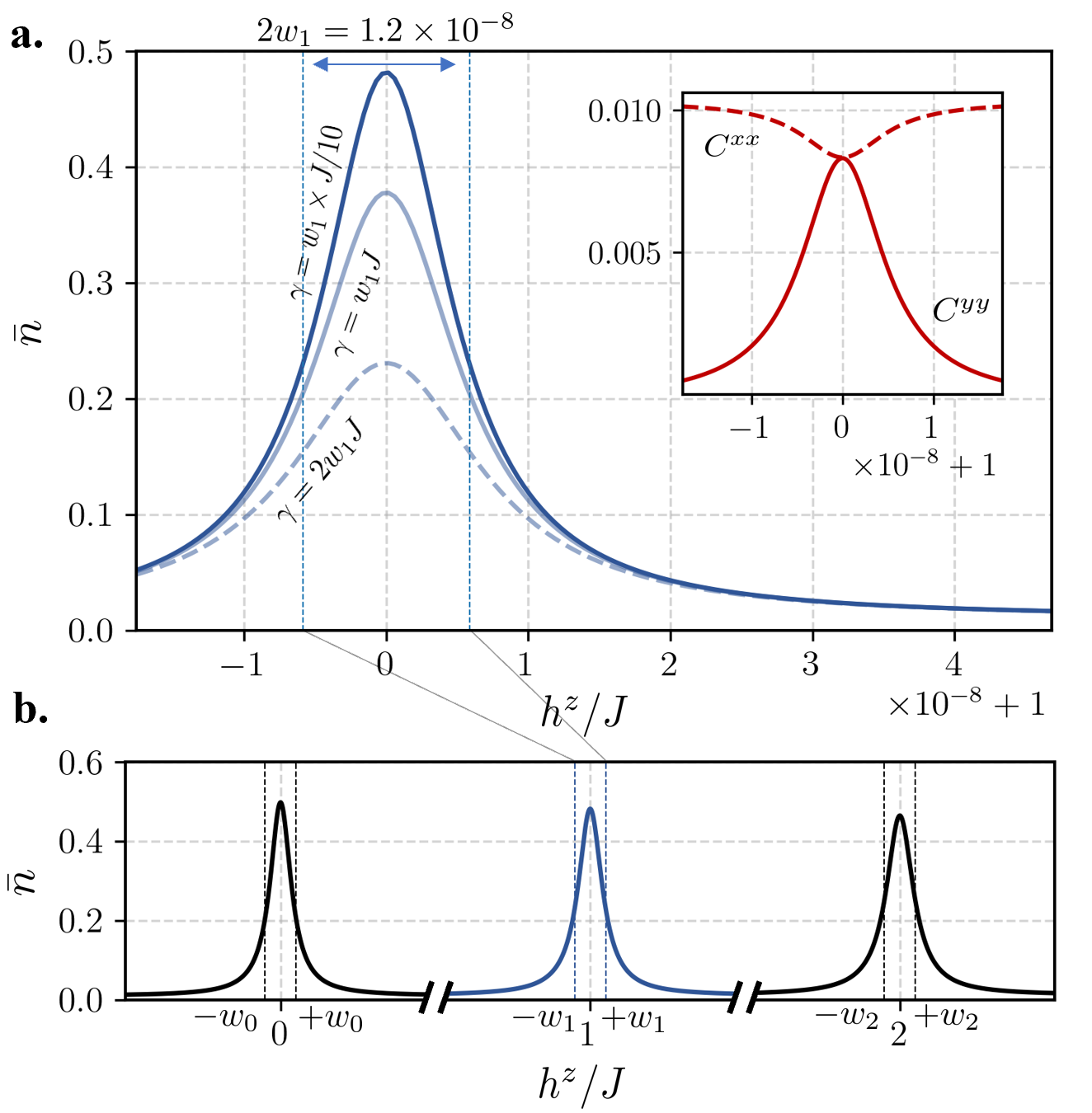
Figure 2: Blockade effect in the dissipative transverse-field Ising model. Top panel (a): plot of the density of up-spins, $\bar{n}=\sum_{j}\langle\hat{\sigma}^{+}_{j}\hat{\sigma}^{-}_{j}\rangle_{\text{SS}}/N$, near a first-order blockade, for $h^{x}=4J$, $\Gamma=0$, and $N=22$. Inset: Plot of the correlation functions $C^{xx}$ (dashed red line) and $C^{yy}$ (solid red line) for the same parameters, where $C^{\mu\mu}:=\langle\hat{\sigma}^{\mu}_{1}\hat{\sigma}^{\mu}_{2}\rangle_{\text{SS}}$. Bottom panel (c): Close-ups of the first three blockades, $n=0,1,2$. Parameters are the same as in panel (b). The exact solution yields extremely precise estimates for the widths of these features, see (12) for more details.

Phase transitions and the large-$N$ limit. At the mean-field level, as one sweeps the longitudinal field $h^{z}$ (corresponding to sweeping the drive-detuning in the driven qubit realization), a spin-configuration with $O(N)$ spins pointing up can become self-consistently resonant, leading to features of a first-order phase transition, such as bistability and hysteresis in the magnetization density Marcuzzi et al. (2014); Carr et al. (2013). Our exact solution yields several new insights into this transition, including the fact that this transition is fundamentally a transition between a polarized and a depolarized state, with the magnetization density serving as a proxy for the amount of polarization in the steady state. The exact solution also allows us to transparently see such a phase transition emerge in the large-$N$ limit, and reveals insights that go beyond mean-field theory, including the location of first-order phase transitions, as well as the behavior of multispin correlations across the transition.

Our starting point is the binomial expansion of $\hat{\Phi}$. Defining $r=h^{z}_{\text{eff}}/J_{\text{eff}}$, this is

$${\hat{\Phi}=}1-r\sum_{k=1}^{N}(1-r)\cdots(k-1-r)\frac{\hat{\mathbb{S}}_{-}^{k}}{k!}.$$ (13)

The relative weight of each monomial $\hat{\mathbb{S}}_{-}^{m}$ in this expansion determines an important piece of physics: if the lowest powers of $\hat{\mathbb{S}}_{-}$ dominate, $\hat{\rho}_{\text{SS}}$ is close to a maximally mixed (depolarized) state, and the magnetization density $m^{\mu}=\langle\hat{M}^{\mu}\rangle/N$ approaches zero. On the other hand, if the highest powers of $\hat{\mathbb{S}}_{-}$ dominate, the steady state is close to a completely polarized state and the (longitudinal) magnetization approaches its minimum value $m^{z}\equiv-1$.

We can make this intuition more precise. We start with the identity $\text{tr}(\hat{\mathbb{S}}_{-}^{\dagger M}\hat{M}^{z}\hat{\mathbb{S}}_{-}^{M^{\prime}})=-M\text{tr}(\hat{\mathbb{S}}_{-}^{\dagger M}\hat{\mathbb{S}}_{-}^{M^{\prime}})$ involving the (longitudinal) magnetization. As a result, we have the somewhat suggestive formula

$$\langle\hat{M}^{z}\rangle_{\text{SS}}=-\frac{\sum_{M}Mp_{M}}{\sum_{M}p_{M}}$$ (14)

where $p_{M}=\|\binom{r}{M}\hat{\mathbb{S}}_{-}^{M}\|^{2}_{\text{HS}}$ is the size of the term proportional to $\hat{\mathbb{S}}_{-}^{M}$ in the expansion of $\hat{\Phi}$ with respect to the Hilbert-Schmidt norm. Eq. (14) makes precise the intuition described above: if the distribution $p_{M}$ is biased towards terms with $M\ll N$, then the magnetization density vanishes in the thermodynamic limit, and the steady state is close to a depolarized state. The opposite occurs when the distribution is skewed towards terms with $M\to N$, in which case the steady state approaches a completely polarized state.

To understand the large-$N$ behavior, we write the magnetization density in the suggestive form

$$m^{z}=-\frac{\sum_{m}m\,e^{-Nf(m)}}{\sum_{m}\,e^{-Nf(m)}},$$ (15)

with $m=M/N$ now a variable ranging between zero and one, representing how polarized the steady state is. Here, $f(m)\equiv-N^{-1}\log p_{Nm}$ is a dimensionless “free energy” that controls the relative weight of the terms in the expansion of $\hat{\Phi}$. To approach the thermodynamic limit, we must hold $\bar{J}_{\text{eff}}:=NJ_{\text{eff}}$ fixed, which fixes the renormalized parameters $\bar{r}:=h^{z}_{\text{eff}}/\bar{J}_{\text{eff}}$, and $\bar{\lambda}_{j}:=2|\bar{J}_{\text{eff}}/h_{j}^{x}|^{2}$.

To make it easier to calculate the free energy, we assume that the transverse fields are uniform, $h_{j}^{x}\equiv h^{x}$. In this case, we have an asymptotic series for $f(m)$ in the large-$N$ limit, with a leading-order contribution

$$f(m) =\log\frac{m^{m}(1-m)^{1-m}}{(m-\bar{r})^{m-\bar{r}}(m-\bar{r}^{*})^{m-\bar{r}^{*}}}-(\log\bar{\lambda}-2)m,$$ (16)

with $O(N^{-1})$ corrections to $f$ given in sup . Since $r$ (and hence $\bar{r}$) cannot be a non-negative real number, $f$ must be an analytic function of $m$. As such, the analytic function $f(m)$ plays an analogous role to an equlibrium free energy in Landau theory Landau (1937), and lets us rigorously describe the phase transition physics in our model.

In particular, the global minima $m^{*}$ of the potential $f$ correspond to the thermodynamic limit $\lim_{N\to\infty}m^{z}$ of the magnetization density. Whenever $f$ has two degenerate global minima, the magnetization density is the average of the two minima, and we have a first-order phase transition from a polarized to a depolarized state, c.f. Fig. 3c. More details can be seen in Fig. 3a, where we also show that the location of the first-order transition line in our model is not accurately predicted by a simple Maxwell construction (indicating the non-equilibrium nature of the model). Whenever the first three derivatives of $f$ vanish at a global minimum, we have a quantum critical point and a second-order phase transition, c.f. Fig. 3b. Note that the formula (15) is still valid for the case of an inhomogeneous magnetic field. In sup , we study these phase transitions in the presence of transverse-field disorder, and also connect them to a sign-change in a particular connected correlation function.

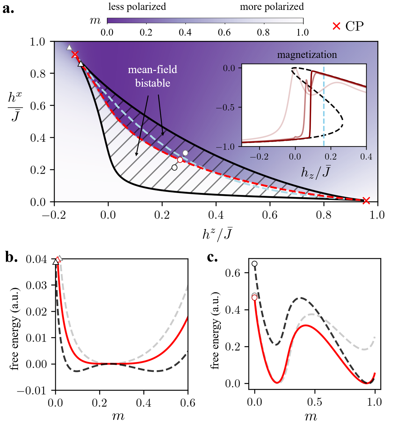
Figure 3: First- and second-order phase transitions in the dissipative transverse-field Ising model. Top panel (a): Steady-state polarization density $m=-\sum_{j}\langle\hat{\sigma}^{z}_{j}\rangle_{\text{SS}}/N$, for $\gamma=\bar{J}/10$, $N=128$, and $\Gamma=0$. The shaded region enclosed by solid black lines denotes parameters where mean field theory predicts bistability. The first-order phase transition occurs when the local minima in $f$ become degenerate, and is traced by a red dashed curve. The location of this transition predicted by the Maxwell construction is given by the blue dashed curve. Critical points where the first three derivatives of $f$ vanish are marked by red crosses. Inset: Steady-state magnetization for $h^{x}=0.4\bar{J}$, and $\gamma=\bar{J}/100$, for $N=4,16,128$. Increasing values of $N$ correspond to increasing opacity. Black dashed curves are used to denote the mean-field solutions. Bottom panel: free energy landscape $f(m)$ determining the amount of polarization $m$ in the steady state $\hat{\rho}_{\text{SS}}$, for three parameter choices near (b) a second-order phase transition, and (c) a first-order phase transition.

Correlation functions. Finally, the exact solution allows one to analytically solve for equal-time correlation functions of arbitrary order in our spin model. For the purpose of succinctly stating the main results, it is useful to define $\hat{\sigma}^{\pm}_{C}\equiv\prod_{j\in C}\hat{\sigma}^{\pm}_{j}$, for $C\subset\{1,2,3,\dots,N\}$ an arbitrary cluster of spins. Given such a cluster, it is convenient to use the notation $C^{c}\equiv\{1,2,3,\dots,N\}\setminus C$ to denote its complement, and $|C|$ to denote its size. Given a pair of clusters $C_{1},C_{2}$, our exact solution yields the expectation value of the normally-ordered product $\hat{\sigma}^{+}_{C_{1}}\hat{\sigma}^{-}_{C_{2}}$. To express the answer in a compact form, we define auxiliary regions $R_{12}=C_{1}\cup C_{2}$, and $R_{j}\equiv(C_{1}\cup C_{2})\setminus C_{j}$. In the situation where the external fields $h^{\mu}$ are uniform, one can express the solution for the expectation value in terms of generalized hypergeometric polynomials:

$$\langle \hat{\sigma}^{+}_{C_{1}}\hat{\sigma}^{-}_{C_{2}}\rangle_{\text{SS}}=\frac{2^{|R_{12}^{c}|}\mathcal{K}^{*}(R_{1})\mathcal{K}(R_{2})}{\mathcal{N}}$$ (17)

$$\times\,_{3}F_{0}(|R_{1}|-r^{*},|R_{2}|-r,|R_{12}|-N;-2|J_{\text{eff}}/h^{x}|^{2}),$$

where $\mathcal{N}=2^{N}\,_{3}F_{0}(-r^{*},-r,-N;-2|J_{\text{eff}}/h^{x}|^{2})$. We have also defined form factors $\mathcal{K}(X)=(-r)_{|X|}\prod_{j\in X}(2J_{\text{eff}}/h_{j}^{x})$, where $(z)_{m}\equiv z(z+1)\cdots(z+m-1)$ is the Pochhammer symbol, or rising factorial .

More generally, in the case of an inhomogeneous field, we obtain the expression

$$\langle\hat{\sigma}^{+}_{C_{1}}\hat{\sigma}^{-}_{C_{2}}\rangle_{\text{SS}} =\frac{2^{|R_{12}^{c}|}\mathcal{K}^{*}(R_{1})\mathcal{K}(R_{2})}{\mathcal{N}}$$ (18)

$$\times\sum_{m}(|R_{1}|-r^{*})_{m}(|R_{2}|-r)_{m}\mathcal{I}_{m}(R_{12}^{c}),$$

where we have defined the form factors $\mathcal{I}_{m}(X)\equiv\sum_{Y\subseteq X,\,|Y|=m}\,\prod_{j\in Y}(2|J_{\text{eff}}/h_{j}^{x}|^{2})$. These form factors satisfy the recursion relation $\mathcal{I}_{m}(X)=\mathcal{I}_{m}(X\setminus\{j\})+2\frac{|J_{\text{eff}}|^{2}}{|h_{j}^{x}|^{2}}\mathcal{I}_{m-1}(X\setminus\{j\})$, which is useful when evaluating the expectation value in the thermodynamic limit.

Summary & Outlook. Here, we present an exact solution for the steady state of a dissipative variant of the infinite-range transverse-field Ising model, including regimes where there is no collective structure or permutation symmetry. We uncover a novel spin blockade effect, and use an effective thermodynamic potential to analytically capture large-$N$ features of the DTI model. While we have focused primarily on the fully-connected transverse-field Ising model, further studies could investigate the steady states of driven-dissipative spin systems defined on graphs with more nontrivial connectivity. In particular, the steady state of the DTI on a $d$-dimensional cubic lattice with $d<\infty$ remains an open problem, and it is interesting to see whether any of the physics we have uncovered in the fully-connected model is also applicable in this more nontrivial regime.

We would like to thank Martin Koppenhoefer and Paul Wiegmann for helpful discussions. This work was supported by the Air Force Office of Scientific Research MURI program under Grant No. FA9550-19-1-0399, and the Simons Foundation through a Simons Investigator award (Grant No. 669487).

References

- Marcuzzi et al. (2014) M. Marcuzzi, E. Levi, S. Diehl, J. P. Garrahan, and I. Lesanovsky, Physical Review Letters 113, 210401 (2014).
- Borish et al. (2020) V. Borish, O. Marković, J. A. Hines, S. V. Rajagopal, and M. Schleier-Smith, Physical Review Letters 124, 063601 (2020).
- Bloch (1946) F. Bloch, Phys. Rev. 70, 460 (1946).
- Jin et al. (2018) J. Jin, A. Biella, O. Viyuela, C. Ciuti, R. Fazio, and D. Rossini, Physical Review B 98, 241108(R) (2018).
- Lee et al. (2012) T. E. Lee, H. Häffner, and M. C. Cross, Physical Review Letters 108, 023602 (2012).
- Kazemi and Weimer (2023) J. Kazemi and H. Weimer, Physical Review Letters 130, 163601 (2023).
- Singh and Weimer (2022) V. P. Singh and H. Weimer, Physical Review Letters 128, 200602 (2022).
- Weimer (2015) H. Weimer, Physical Review A 91, 063401 (2015).
- Overbeck et al. (2017) V. R. Overbeck, M. F. Maghrebi, A. V. Gorshkov, and H. Weimer, Physical Review A 95, 042133 (2017).
- Carr et al. (2013) C. Carr, R. Ritter, C. G. Wade, C. S. Adams, and K. J. Weatherill, Physical Review Letters 111, 113901 (2013).
- Malossi et al. (2014) N. Malossi, M. M. Valado, S. Scotto, P. Huillery, P. Pillet, D. Ciampini, E. Arimondo, and O. Morsch, Physical Review Letters 113, 023006 (2014).
- Paris-Mandoki et al. (2017) A. Paris-Mandoki, C. Braun, J. Kumlin, C. Tresp, I. Mirgorodskiy, F. Christaller, H. P. Büchler, and S. Hofferberth, Physical Review X 7, 041010 (2017).
- Britton et al. (2012) J. W. Britton, B. C. Sawyer, A. C. Keith, C.-C. J. Wang, J. K. Freericks, H. Uys, M. J. Biercuk, and J. J. Bollinger, Nature 484, 489 (2012).
- Ebadi et al. (2021) S. Ebadi, T. T. Wang, H. Levine, A. Keesling, G. Semeghini, A. Omran, D. Bluvstein, R. Samajdar, H. Pichler, W. W. Ho, S. Choi, S. Sachdev, M. Greiner, V. Vuletić, and M. D. Lukin, Nature 595, 227 (2021).
- Scholl et al. (2021) P. Scholl, M. Schuler, H. J. Williams, A. A. Eberharter, D. Barredo, K.-N. Schymik, V. Lienhard, L.-P. Henry, T. C. Lang, T. Lahaye, A. M. Läuchli, and A. Browaeys, Nature 595, 233 (2021).
- Foss-Feig et al. (2013) M. Foss-Feig, K. R. A. Hazzard, J. J. Bollinger, and A. M. Rey, Physical Review A 87, 042101 (2013).
- McDonald and Clerk (2022) A. McDonald and A. A. Clerk, Physical Review Letters 128, 033602 (2022).
- Roberts et al. (2021) D. Roberts, A. Lingenfelter, and A. A. Clerk, PRX Quantum 2, 020336 (2021).
- Fagnola and Umanità (2010) F. Fagnola and V. Umanità, Communications in Mathematical Physics 298, 523 (2010).
- Paz and Maghrebi (2021) D. A. Paz and M. F. Maghrebi, Physical Review A 104, 023713 (2021).
- Huybrechts et al. (2020a) D. Huybrechts, F. Minganti, F. Nori, M. Wouters, and N. Shammah, Physical Review B 101, 214302 (2020a).
- Lee and Chan (2013) T. E. Lee and C.-K. Chan, Physical Review A 88, 063811 (2013).
- Ates et al. (2012) C. Ates, B. Olmos, J. P. Garrahan, and I. Lesanovsky, Physical Review A 85, 043620 (2012).
- Carollo and Lesanovsky (2021) F. Carollo and I. Lesanovsky, Phys. Rev. Lett. 126, 230601 (2021).
- Fiorelli et al. (2023) E. Fiorelli, M. Müller, I. Lesanovsky, and F. Carollo, New Journal of Physics 25, 083010 (2023), publisher: IOP Publishing.
- Huybrechts et al. (2020b) D. Huybrechts, F. Minganti, F. Nori, M. Wouters, and N. Shammah, Physical Review B 101, 214302 (2020b), arxiv:1912.07570 [cond-mat, physics:quant-ph] .
- Jo et al. (2022) M. Jo, B. Jhun, and B. Kahng, “Resolving mean-field solutions of dissipative phase transitions using permutational symmetry,” (2022), arxiv:2110.09435 [cond-mat, physics:quant-ph] .
- Kelley (1979) F. Kelley, Reversibility and Stochastic Networks (Cambridge University Press, 1979).
- Fagnola and Umanita (2007) F. Fagnola and V. Umanita, Infinite Dimensional Analysis, Quantum Probability and Related Topics 10, 335 (2007).
- (30) See Supplemental Material (SM) for more theoretical details. The SM includes Refs. Goldstein and Lindsay (1995); Fagnola and Umanita (2007); Ramezani et al. (2018); Fagnola and Umanità (2010); Evans (1977); Roberts and Clerk (2023); Huybrechts et al. (2020b).
- Puri and Lawande (1979) R. R. Puri and S. V. Lawande, Physics Letters A 72, 200 (1979).
- Drummond (1980) P. D. Drummond, Physical Review A 22, 1179 (1980).
- Lawande et al. (1981) S. V. Lawande, R. R. Puri, and S. S. Hassan, Journal of Physics B: Atomic and Molecular Physics 14, 4171 (1981).
- Schneider and Milburn (2002) S. Schneider and G. J. Milburn, Physical Review A 65, 042107 (2002).
- Nagy et al. (2010) D. Nagy, G. Kónya, G. Szirmai, and P. Domokos, Physical Review Letters 104, 130401 (2010).
- Hannukainen and Larson (2018) J. Hannukainen and J. Larson, Phys. Rev. A 98, 042113 (2018).
- Landau (1937) L. D. Landau, Phys. Z. Sowjet. 11, 26 (1937).
- Note (1) In this case, the external fields are uniform, and so we can use the simpler formula .
- Goldstein and Lindsay (1995) S. Goldstein and J. M. Lindsay, Mathematische Zeitschrift 219, 591 (1995).
- Ramezani et al. (2018) M. Ramezani, F. Benatti, R. Floreanini, S. Marcantoni, M. Golshani, and A. T. Rezakhani, Physical Review E 98, 052104 (2018).
- Evans (1977) D. E. Evans, Communications in Mathematical Physics 54, 293 (1977).
- Roberts and Clerk (2023) D. Roberts and A. A. Clerk, Phys. Rev. Lett. 130, 063601 (2023).