Reliability of Noisy Quantum Computing Devices

Abstract.

Noisy intermediate-scale quantum (NISQ) devices are valuable platforms for testing the tenets of quantum computing, but these devices are susceptible to errors arising from de-coherence, leakage, cross-talk and other sources of noise. This raises concerns for ensuring the stability of program results when using NISQ devices as strategies for mitigating errors generally require well-characterized and reliable error models. Here, we quantify the reliability of NISQ devices by assessing the necessary conditions for generating stable results within a given tolerance. We use similarity metrics derived from device characterization data to analyze the stability of performance across several key features: gate fidelities, de-coherence time, SPAM error, and cross-talk error. We bound the behavior of these metrics derived from their joint probability distribution, and we validate these bounds using numerical simulations of the Bernstein-Vazirani circuit tested on a superconducting transmon device. Our results enable the rigorous testing of reliability in NISQ devices and support the long-term goals of stable quantum computing.

This manuscript has been authored by UT-Battelle, LLC under Contract No. DE-AC05-00OR22725 with the U.S. Department of Energy. The United States Government retains and the publisher, by accepting the article for publication, acknowledges that the United States Government retains a non-exclusive, paid-up, irrevocable, worldwide license to publish or reproduce the published form of this manuscript, or allow others to do so, for United States Government purposes. The Department of Energy will provide public access to these results of federally sponsored research in accordance with the DOE Public Access Plan (https://www.energy.gov/doe-public-access-plan).

1. Introduction

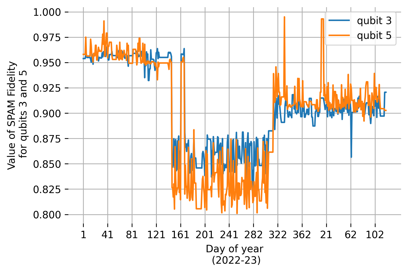
Figure 1. Daily estimates of the state preparation and measurement fidelity for two register elements in a superconducting transmon device collected from 1-Jan-2022 to 30-Apr-2023 (aleksandrowicz2019qiskit, ). Day of the year is indexed starting with 1 and index 365 corresponds to Dec 31.

Daily estimates of the state preparation and measurement fidelity for two register elements in a superconducting transmon device.

Ongoing efforts to realize the principles of quantum computing have demonstrated control over quantum physical systems ranging from superconducting electronics (burnett2019decoherence, ), trapped ions (wan2019quantum, ), and silicon quantum dots (PhysRevApplied.10.044017, ) among many others (humble2019quantum, ). As these efforts aim for future fault-tolerant operation (gottesman1998theory, ), they have established a regime of noisy, intermediate-scale quantum (NISQ) devices that provide a frontier for testing the principles of quantum computing under experimental conditions (preskill2019quantum, ). Such first-in-kind NISQ computing devices enable design verification (PhysRevA.101.042315, ), device characterization (harper2020efficient, ), program validation (ferracin2019accrediting, ), and a breadth of testing and evaluation for application performance (kandala2017hardware, ; dumitrescu2018cloud, ; hempel2018quantum, ; klco2018quantum, ; mccaskey2019quantum, ; roggero2020quantum, ) with several recent demonstrations exemplifying the milestone of quantum computational advantage (arute2019, ; google2020hartree, ; zhong2020quantum, ).

A prominent feature of experimental NISQ computing is that noise and errors limit performance (martinis2015qubit, ) such that a device must be frequently calibrated to maintain high-fidelity operations. Many different metrics are used for monitoring noise within NISQ devices and informing benchmarking methods that assess the accuracy of noisy quantum computation (eisert2020quantum, ; BlumeKohout2020volumetricframework, ; lilly2020modeling, ). These metrics are also essential for mitigating noise-induced errors (temme2017error, ; kandala2019error, ; rudinger2019probing, ; geller2020rigorous, ; wilson2020just, ; hamilton2020error, ), (PhysRevLett.78.3971, ; PhysRevA.94.032321, ). Error-mitigated benchmarks establish bounds on the statistical significance of experimental demonstrations using NISQ devices and help clarify the conditions under which results are reproducible (proctor2022measuring, ).

There are different temporal and spatial scales on which to describe the noise sources affecting the fidelity of quantum computing devices. Noise sources that act on the time scale of a single gate operation notably create errors that are observed during an individual quantum circuit execution, while variations in the noise process over minutes and days influence experimental reproducibility (mcrae2021reproducible, ; burnett2019decoherence, ; schultz2022impact, ; etxezarreta2021time, ; demarti2022performance, ; gulacsi2023smoking, ). For example, Fig. 1 shows an example of daily fluctuations in the estimated state preparation and measurement (SPAM) fidelity from two register elements in a superconducting transmon device for a 16-month period (washington, ). Changes in key metrics arise from various factors including unintentional drift in the control system as well as intentional changes in how the device is operated (proctor2020detecting, ; van_Enk_2013, ; PhysRevApplied.15.014023, ; PhysRevLett.78.3971, ), and how to manage and mitigate fluctuations across these longer scales is an outstanding concern.

In experiments utilizing NISQ devices, it is often necessary to estimate circuit outcomes using a large number of samples, ranging from thousands to millions, and these experiments can span minutes to hours to days depending on the technology and application. While error mitigation methods exist to handle the stationary noise processes assumed during these executions, there is a gap in methods available to account for non-stationary noise processes. Hardware-aware compilation methods (kandala2017hardware, ) can be used to mitigate some slower fluctuations, but this fails to address whether an observed result can be reproduced elsewhere or by others. Stability is a serious concern for current quantum benchmarking methods, which do not account for the transient nature of device noise nor provide a means to assess how these fluctuations impact the results (etxezarreta2021time, ). In order to ensure the stability of benchmarking results across changes in the underlying devices, the reliability of the device itself must be assessed.

Assessing the reliability of NISQ devices complements concurrent efforts to evaluate the accuracy, stability, and reproducibility of quantum computing. Accuracy is used widely to quantify how well an instance of an experimentally observed output from noisy circuit execution matches a known expected outcome (ferracin2021experimental, ; kliesch2021theory, ; bravyi2021mitigating, ; blume2010optimal, ; blume2020modeling, ; lilly2020modeling, ; maciejewski2021modeling, ; geller2020rigorous, ; hamilton2020error, ; hamilton2020scalable, ), while stability measures whether the program behavior stays bounded in the presence of noise fluctuations (dasgupta2022assessing, ). By comparison, reliability quantifies the statistical similarity of the underlying device parameters, such as gate fidelities, across multiple program instances, and reproducibility quantifies the similarity between instances of the program output with previously executed instances on the same or different devices (dasgupta2021reproducibility, ).

Here we formalize the concept of device reliability as a measure of similarity between characterizations of device performance, and use the resulting similarity distance to establish bounds on the likelihood that noisy quantum circuits will yield outcomes that are statistically similar. In Sec. 2, we catalog a subset of metrics that represent key criteria for quantum computation and derive bounds on device reliability for outcomes of programs executed on NISQ devices. In Sec. 3, we apply statistical testing of the distance metric to assess when a device is reliable using the temporal and spatial reliability of a 127-qubit transmon device as an example. In Sec. 4, we validate the reliability bound for an implementation of the Bernstein-Vazirani circuit using characterization data. We conclude in Sec. 5, with a summary of the key findings.

2. Theoretical Model

Consider an idealized quantum computer composed of an $n$-qubit register that encodes a $2^{n}$-dimensional Hilbert space $(\mathbb{C}^{2})^{\otimes n}$ and a set of operations that transform the register state. Projective operations initialize the state of the register, e.g., in the computational basis state as $\ket{\psi}=\ket{0}^{\otimes n}$, while a unitary operation, or gate, $\mathcal{U}$ transforms the state as $\ket{\psi}\rightarrow\mathcal{U}\ket{\psi}$. Additional projective operations implement the measurement of the quantum register. Let $\ket{v}$ denote a register state in the computational basis where $v\in\{0,1\}^{n}$. The probability to observe the outcome $\ket{v}$ is given by $\textrm{Pr}(v)=|\braket{v}{\mathcal{U}}{\psi}|^{2}$. A quantum circuit expresses a discrete sequence of unitary and projective operations acting upon the register, and a quantum program executed by a quantum control unit issues such circuits during operation of the quantum computer.

2.1. Characterizing NISQ Devices

Practical efforts to realize a quantum computer encounter multiple sources of noise and error that make the description above approximate at best (kliesch2021theory, ; ferracin2021experimental, ; coveney2021reliability, ; blume2010optimal, ). For example, the physical realization of the quantum register is subject to noise processes such as decay and de-coherence, coupling to the environment, intra-register cross-talk, and computational leakage. This reduces the lifetime for storing quantum information and produces unintended interactions during the computation. In addition, the implementation of physical operations, such as gates and measurements, rely on analog fields that are subject to pulse distortion, attenuation, jitter, and drift. The processes distort the intended control fields and reduce the fidelity of preparation, measurement, single-qubit rotations and two-qubit entangling gates. Changes in thermodynamic controls such as cryogenic cooling, electromagnetic shielding, vibration suppression, and vacuum, are also subject to uncontrolled fluctuations that disturb the operating conditions and environment of the quantum computing device.

Metric (Symbol)	Description
Capacity ($n$)	Maximal amount of information that may be stored in the register
SPAM Fidelity ($F_{\textrm{I}}$)	Accuracy with which a fiducial register state is prepared and measured
Gate Fidelity ($F_{\textrm{G}}$)	Accuracy with which a gate transforms the register state.
Duty Cycle ($\tau_{G}$)	Ratio of gate duration to de-coherence time
Addressability ($F_{\textrm{A}}$)	Measure of correlation in readout

Table 1. A listing of the five device metrics used for evaluating NISQ computation.

Device Calibration Metrics

Characterizing the influence of noise on the operation of a NISQ computing device requires monitoring a variety of diagnostic metrics. Many characterization metrics are specific to the technology being considered, but there is a subset of five key metrics shown in Table 1 that represent the criteria established by DiVincenzo for achieving a functional quantum computer (divincenzo2000physical, ). This includes fixed quantities, such as the capacity $n$ of the quantum register, i.e., number of qubits, as well as tunable quantities, such as the time it takes to execute a specific quantum gate (also called gate duration) while other metrics characterize noise processes such as the fidelities of individual operations. There are a variety of characterization methods for estimating these metrics, and the specific choice depends on the desired precision and characterization time (sheldon2016characterizing, ; erhard2019characterizing, ; blume2020modeling, ; magesan2012characterizing, ; mcrae2021reproducible, ). We next review each of these metrics.

2.1.1. SPAM fidelity

State preparation and measurement fidelity $F_{\text{SPAM}}$ quantifies the accuracy with which a target quantum state is prepared and measured in the register and this can be quantified by the quantum state fidelity. Tomographic methods are informative for measuring the fidelity of general quantum states but these approaches typically scale steeply with the size of the register (aaronson2019shadow, ). An alternative method measures the fidelity of a more restrictive set of states, which in the extreme limit, may be reduced to characterizing a fiducial computational basis state, such as $|0\rangle^{\otimes n}$. A simple and highly efficient characterization defines the state preparation and measurement (SPAM) fidelity $F_{\text{SPAM}}$ as the probability to measure the $n$-bit string matching the fiducial state and the error $\epsilon_{\text{SPAM}}$ as the probability of observing any other outcome:

(1) $$F_{\text{SPAM}}\coloneqq 1-\epsilon_{\text{SPAM}}.$$

Notably, readout error is implicitly included in this characterization method.

2.1.2. Gate Fidelity

Gate fidelity $F_{G}$ measures the accuracy with which a quantum operation transforms the register state. Many methods (chuang1997prescription, ; emerson2005scalable, ; knill2008randomized, ; gambetta2012characterization, ; mckay2019three, ) have been developed to characterize noise in gate operations, and we limit consideration to randomized benchmarking applied to characterization of the 2-qubit Clifford group as it is a scaleable protocol in principle (although it does not give a complete description of the noise). Randomized benchmarking is widely used to measure the quantum state survival probability following a sequence of randomly selected Clifford elements by fitting the resulting sequence of fidelity measurements to a linear model that eliminates the influence of state preparation and measurement errors (magesan2011scalable, ). These parameters are then used to estimate the average error per Clifford gate with more sophisticated methods, such as interleaved randomized benchmarking, capable of estimating the error of a specific gate. The resulting gate fidelity $F_{G}\coloneqq$ is defined by the error per Clifford gate $\epsilon_{G}$:

(2) $$F_{G}\coloneqq 1-\epsilon_{G}.$$

Due to its significant impact on the overall performance of modern quantum computing devices, we focus our attention specifically on characterizing the two-qubit CNOT operation, as it often plays a decisive role in the performance limits of NISQ computing.

2.1.3. Duty Cycle

Alongside gate fidelity is the important consideration of gate duration relative to register de-coherence time. Register de-coherence time is the duration or timescale during which the quantum register maintains its ability to exhibit interference effects and preserve the delicate relationships between quantum states (e.g. maintain an entangled state, undisturbed by external influences). Gate duration is the time needed to drive the intended coherent interaction. A longer coherence time relative to gate duration allows for a more robust quantum information processing (gambetta2019, ). Gate fidelity can often be improved by lengthening the duration of the control interaction, but this necessarily reduces the number of such operations that can be performed within a given de-coherence time. The de-coherence time, represented by the $T_{2}$ time, is determined using the standard Hahn echo technique. It measures the time it takes for a qubit to lose its coherence. The decay of coherence can be described by an exponential function with the characteristic constant $T_{2}$. We define the duty cycle $\tau_{G}$ as the ratio of the register de-coherence time to the duration $T_{G}$ of a given gate

(3) $$\tau_{G}\coloneqq T_{2}/T_{G}.$$

Both $T_{2}$ and $T_{G}$ may undergo fluctuations, but the composite metric $\tau_{G}$ measures the number of gates that can be executed within the de-coherence time available, providing a quantification of the circuit depth achievable.

2.1.4. Addressability

Addressability characterizes how well each register element can be measured individually, and we quantify this in terms of the pair-wise correlations that arise during measurement in the computational basis. Although qualitatively this has been discussed in a few places e.g. (perez2011quantum, ), there is not much existing literature on this metric. Correlated errors occur during either unitary or projective operations due to cross-talk that couples transformations of the quantum state. We quantify the correlations between the measurement outcomes $X$ and $Y$ using the mutual information $\mathcal{I}(X,Y)$, and we define the normalized mutual information

(4) $$\eta(X,Y)\coloneqq\frac{2\mathcal{I}(X,Y)}{\mathcal{H}(X)+\mathcal{H}(Y)},$$

with $\mathcal{H}(X)$ the entropy of the discrete random variable $X$. The resulting addressability fidelity is

(5) $$F_{A}\coloneqq 1-\eta.$$

The addressability depends on the initial correlations within the quantum state. For example, any separable pure state yields unit fidelity while the addressability of a maximally entangled state vanishes due to correlated outcomes.

2.2. Measuring Device Reliability

The metrics described above characterize essential features for how a quantum computer operates. Other metrics must also be considered when characterizing a specific device or technology. We quantify device reliability by comparing statistical distributions for the characterization metrics collected at different times and register locations. If the characterization metrics are statistically similar, then the behavior of the device itself is reliable. The metrics themselves may be compared by calculating the statistical distance, or similarity, between their distributions. There are several measures suitable for quantifying statistical distance, and we use the Hellinger distance to validate these ideas due to its relative ease of calculation and interpretation.

The Hellinger distance is a similarity measure between the probability distributions $f_{X}(\textrm{x})$ and $f_{Y}(\textrm{x})$ for random variables $X$ and $Y$. It is given by

(6) $$H(f_{X},f_{Y})\coloneqq\sqrt{1-BC(f_{X},f_{Y})},$$

where the Bhattacharyya coefficient BC is

(7) $$BC(f_{X},f_{Y})\coloneqq\int\limits_{\textrm{x}}\sqrt{f_{X}(\textrm{x})f_{Y}(\textrm{x})}d\textrm{x}.$$

Here $f_{X}(\textrm{x})$ and $f_{Y}(\textrm{x})$ are the distribution functions for the real-valued random variables $X$ and $Y$ respectively. In particular, x is a realization of the random multi-dimensional variable $X$ drawn from the time-varying distribution $f_{X}(\textrm{x};t)$, where $t$ denotes time. The Hellinger distance is bounded between 0 and 1 and symmetric with respect to the inputs. It vanishes for identical distributions and approaches unity for distributions with no overlap. We will show that the Hellinger distance quantifies fluctuations between device metrics as well as the underlying quantum states. The latter holds because the Hellinger distance between the measurement outcomes of a quantum circuit provides a lower bound on the distance between the underlying quantum states (jarzyna2020geometric, ).

Unlike a comparison of averages, the similarity distance evaluates changes in the shape of the distribution with respect to a time-varying noise process and, therefore, is a more demanding test of device reliability. Consider $f_{X}(\textrm{x};t)$ to be the distribution of metric $X$ characterized at time $t$, and let

(8) $$H_{X,Y}(t_{1},t_{2})\coloneqq H(f_{X}(t_{1}),f_{Y}(t_{2})),$$

measure the distance between the distribution of $X$ at time $t_{1}$ and the distribution of $Y$ at time $t_{2}$. Thus, the Hellinger distance in Eqn. 8 is defined even when characterization of a distribution necessitates a series of measurements.

The definition may be simplified further for the case of self-similarity when $X=Y$ such that $H_{X,Y}=H_{X}$. For example, $H_{F_{\text{SPAM}}}(t_{1},t_{2})$ measures the similarity in distributions of SPAM fidelity at different times. A reliable, but not necessarily ideal, device maintains the characteristic distribution for the fidelity at both times. By similar considerations, spatially-varying noise processes are captured by this definition. Consider metrics $X=F_{G}^{(i)}$ and $Y=F_{G}^{(j)}$ to represent the gate fidelity for register connections $i$ and $j$, respectively. The resulting distance, abbreviated $H_{F_{G}^{(i,j)}}(t_{1},t_{2})$, quantifies differences in the gate fidelities at these locations. For any of these realization of the similarity metric, we call a device $\varepsilon$-reliable in metrics $X$ and $Y$ when

(9) $$H_{X,Y}<\varepsilon$$

Despite its ease of interpretation, the Hellinger distance scales exponentially in the number of circuit noise parameters. This has the effect that even small changes in a distribution will yield large changes in the distance value. This will be discussed further in Section A.3. Presently, it suffices to note that the sensitivity of the reliability test $H_{X}(t_{1},t_{2})<\varepsilon$ is correspondingly decreases with increasing dimensionality of the device characterization. Instead, we define a more sensitive test for reliability by using $H_{\textrm{avg}}$, defined as the average over the distances for the $d$ univariate $(X_{k})$ marginal distributions:

(10) $$H_{\textrm{avg}}(t_{1},t_{2})\coloneqq\frac{1}{d}\sum\limits_{k=1}^{d}H_{X_{k}}(t_{1},t_{2}).$$

When the joint distributions are time-invariant, then the marginals must also be time-invariant, resulting in a small average value for $H_{\textrm{avg}}$. This test is more sensitive as it mitigates the curse of dimensionality and offers higher dispersion for improved calibration. Another equally sensitive approach is to normalize the total distance relative to the dimensionality $d$ of the distribution:

(11) $$H_{\textrm{normalized}}(t_{1},t_{2})\coloneqq\sqrt{1-BC^{1/d}}.$$

We refer to this statistic as the normalized Hellinger distance (note that although we call it distance, this statistic is not a metric as it does not satisfy the triangle inequality).

2.3. Bounds on Reliability

We have defined device reliability as a measure of the similarity between device metrics with respect to spatially and time-varying noise processes. We next consider how reliability bounds the outcomes of programs executed on NISQ devices by comparing changes in program output relative to fluctuations in the device metrics.

Consider the initial state of an $n$-qubit register described by the density matrix $\rho_{\textrm{in}}$ to be transformed by a noiseless circuit $C$

(12) $$C=\mathcal{U}_{L}\cdots\mathcal{U}_{1},$$

comprising $L$ unitaries (also called gates) $\mathcal{U}_{1},\cdots,\mathcal{U}_{L}$. The effect of noise during execution of the circuit on a noisy quantum device is represented by the composite error channel $\mathcal{E}_{X}(\cdot):$

(13) $$\rho_{\textrm{out}}^{\textrm{noisy}}=\mathcal{E}_{\textrm{x}}\left(\rho_{out}^{\textrm{ideal}}\right),$$

where $\rho_{out}^{\textrm{ideal}}$ is the ideal output from a quantum circuit executed on a noiseless device and x is a vector of device parameters $(\textrm{x}_{1},\cdots,\textrm{x}_{d})$ consistent with previous notation.

Now let $O$ denote the operator for an observable computed from the output of the quantum circuit $C$. The operator has the spectral decomposition

$$O=\sum\limits_{m}\lambda_{m}\ket{\lambda_{m}}\bra{\lambda_{m}}$$

where $\lambda_{m}$ are the real eigenvalues of $O$ and $\ket{\lambda_{m}}$ denote the eigenstates. The expectation value of the observable $O$ with respect to the (noisy) quantum state described by the density matrix $\rho_{\textrm{out}}^{\textrm{noisy}}$ is:

(14) $$\braket{O_{\textrm{x}}}=\textrm{Tr}\left(O\rho_{\textrm{out}}^{\textrm{noisy}}\right)=\textrm{Tr}\left(O\mathcal{E}_{\textrm{x}}(\rho_{\textrm{out}}^{\textrm{ideal}})\right)=\sum\limits_{m}\lambda_{m}\textrm{Tr}\left(\Pi_{m}\mathcal{E}_{\textrm{x}}(\rho_{\textrm{out}}^{\textrm{ideal}})\right),$$

where $\Pi_{m}=\ket{\lambda_{m}}\bra{\lambda_{m}}$ is the projective operator.

The value $\braket{O_{\textrm{x}}}$ is relative to a single fixed instance of the parameter x. However, in NISQ computing, an expectation value represents an average over x with respect to the distribution $f_{X}(\textrm{x};t)$ that varies with time. Let us define the average of $\braket{O_{\textrm{x}}}$ with respect to the $f_{X}(\textrm{x};t)$ as:

(15) $$\braket{O}_{t}\coloneqq\int\limits\braket{O_{\textrm{x}}}f_{X}(x;t)d\textrm{x}.$$

In the absence of knowledge of the exact realization of x at time t, $\braket{O}_{t}$ is an estimate for the mean of the observable in presence of time-varying noise channels.

Let $s(t_{1},t_{2})$ be the absolute difference in the mean of the observable obtained from the noisy quantum device at times $t_{1}$ and $t_{2}$:

(16) $$s(t_{1},t_{2})\coloneqq|\braket{O}_{t_{1}}-\braket{O}_{t_{2}}|.$$

We will refer to $s(t_{1},t_{2})$ as the stability of the mean of the observable between times $t_{1}$ and $t_{2}$, or observable stability for short (dasgupta2021stability, ). As shown in Appendix A.1, the observable stability is upper bounded by:

(17) $$s_{\textrm{max}}=2cH_{X}\sqrt{2-H_{X}^{2}},\;\;\;\;\textrm{where}\;\;\;\;c=\underset{\textrm{x}}{\textrm{sup}}|\braket{O_{\textrm{x}}}|.$$

Note the constant $c$ has no dependence on the time-varying distribution $f_{X}(\textrm{x};t)$ and for notational clarity, we have used:

(18) $$H_{X}^{2}=H^{2}_{X}(t_{1},t_{2})=1-\int\sqrt{f_{X}(\textrm{x};t_{1})}\sqrt{f_{X}(\textrm{x};t_{2})}dx.$$

Alternately, using Eqn. 11, the maximum of the obervable stability can also be expressed as:

(19) $$s_{\textrm{max}}=2cH_{X}\sqrt{2-H_{X}^{2}}=2c\sqrt{1-\left[BC^{(1/d)}\right]^{2d}}=2c\sqrt{1-(1-H_{\textrm{normalized}}^{2})^{2d}}.$$

Equations 17 and 19 upper bound the temporal variations in the expected mean of the circuit outcome with respect to the statistical reliability of the device metrics. As expected, the temporal variations vanish when $H_{X}=0$ and become maximal when $H_{X}=1$. The bound itself is monotonic in the Hellinger distance, with the greatest change occurring for the greatest distance. This bounds the time-variation of the average program output as a function of the readily available device characterization data.

2.4. Example Application

In this section, we verify Eqn. 17 using numerical simulations with time-varying depolarizing noise.

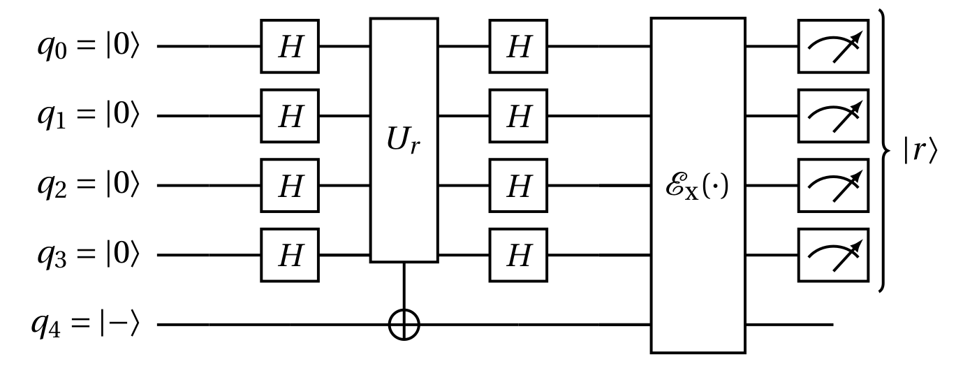
Figure 2. A quantum circuit implementation of the Bernstein-Vazirani algorithm that employs 5 qubits, denoted $q_{0}$ to $q_{4}$. The first four qubits are used to compute the 4-bit secret string, while the fifth qubit serves as an ancilla and initially resides in the $\ket{-}$ superposition state. The symbol $H$ denotes the Hadamard gate while the oracle unitary ($U_{r}$) implements the secret string ($r$). The depolarizing noise channel is denoted by $\mathcal{E}_{\textrm{x}}(\cdot)$. A quantum measurement operation is represented by the meter box symbol at the circuit’s end. The corresponding implementation using Qiskit is shown in Fig. 9 of the Appendix.

Quantum circuit for the implementation of the Bernstein-Vazirani algorithm.

Our example evaluates the bound on a noisy circuit implementation of the Bernstein-Vazirani algorithm (bernstein1993quantum, ). This algorithm returns the secret $n$-bit string $r$ encoded into an oracle

(20) $$f^{\textrm{BV}}(z)=z\cdot r,$$

by making as few queries as possible. The best classical method requires $n$ queries of the oracle while exactly one query is required for the Bernstein-Vazirani algorithm. The quantum circuit for a 4-bit secret key is shown in Fig. 2 in which $U_{r}$ implements the oracle unitary.

For the Bernstein-Vazirani problem, we are interested in the probability of success to compute the secret bit string $r$ where $\ket{r}=\bigotimes\limits_{i=1}^{n}\ket{r_{i}}$ with $r_{i}\in\{0,1\}$. The observable for the problem is:

(21) $$\begin{split}O&=\Pi_{r}=\ket{r}\bra{r}.\end{split}$$

The state for the ideal, noiseless circuit is $\rho_{\textrm{out}}^{\textrm{ideal}}=\ket{r}\bra{r}$ and, hence, the corresponding probability of success for the noisy circuit describe in Fig. 2 is

(22) $$\textrm{ Pr(r) = Tr}\left[\Pi_{r}\mathcal{E}_{\textrm{x}}(\ket{r}\bra{r})\right].$$

For simplicity, our noise model assumes each register element is acted upon by isotropic depolarizing noise, such that the superoperator $\mathcal{E}_{\textrm{x}}(\cdot)$ represents the tensor product of independent single-qubit isotropic depolarizing channels. The $i$-th such channel is modeled as:

(23) $$\begin{split}\mathcal{E}_{\textrm{x}_{i}}(\rho)&=\left(1-\frac{3\textrm{x}_{i}}{4}\right)\rho+\frac{\textrm{x}_{i}}{4}(\mathds{X}_{i}\rho\mathds{X}_{i}+\mathds{Y}_{i}\rho\mathds{Y}_{i}+\mathds{Z}_{i}\rho\mathds{Z}_{i})\end{split}$$

where $\textrm{x}_{i}$ is the depolarizing parameter for the i-th register element’s noise channel and $\mathds{X}_{i}$, $\mathds{Y}_{i}$, and $\mathds{Z}_{i}$ are the Pauli matrices acting on the $i$-th register element. Further, let $\textrm{x}_{i}$ be a particular realization of the random variable $X_{i}$, sampled from the multi-variate joint distribution $f_{X}(\textrm{x};t)$ which has $d$ random variables characterizing the noise in circuit $C$. We will further assume that the $\{X_{i}\}$ can have correlations in their values. The univariate marginal distribution for the random variable $X_{i}$ is denoted by $f_{X_{i}}(\textrm{x}_{i};t)$ where $i\in(1,\cdots,d)$. In this specific example, $d=n$.

As discussed before, let $\braket{O_{\textrm{x}}}$ denote the mean of the observable in presence of a (depolarizing) noise channel with static (time-invariant) noise. Assuming the noise channel is separable but correlated:

(24) $$\begin{split}\braket{O_{\textrm{x}}}&=\prod_{i=1}^{d}\left(1-\frac{\textrm{x}_{i}}{2}\right).\end{split}$$

We will next explore the statistical modeling details of time-varying depolarizing noise, which will be applied in numerical simulations of the Bernstein Vazirani circuit as a working example to investigate the connection between device reliability and program output stability.

2.4.1. Time-varying depolarizing channel

As a specific instance of a time-varying depolarizing channel, suppose the noise marginals stay constant in the mean while the variance increases linearly with time:

(25) $$\begin{split}\mathds{E}(\textrm{x}_{i})=&\mu_{0}\;\;\;\;\forall i,t\\ \textrm{Var}(\textrm{x}_{i})=\sigma_{t}^{2}=&\sigma_{0}^{2}\left(1+(\omega-1)\frac{t}{T}\right)\;\;\;\;\forall i,\end{split}$$

where $\omega=\sigma^{2}_{T}/\sigma^{2}_{0}$ is a constant capturing how volatile the distribution becomes at time $T$ compared to initial time t=0 and $i$ denotes the register number. Classical correlation in the noise is modeled by the correlation matrix $\Sigma$ where $\Sigma_{ij}$ represents the correlation coefficient between the depolarizing parameter $X_{i}$ acting on register element $i$ and $X_{j}$ acting on register element $j$.

We use a beta distribution to represent the marginal distribution of the depolarizing parameter $\textrm{x}_{i}$ as

(26) $$f_{X_{i}}(\textrm{x}_{i};t)=\frac{\textrm{x}_{i}^{\alpha_{t}-1}(1-\textrm{x}_{i})^{\beta_{t}-1}}{\textrm{Beta}(\alpha_{t},\beta_{t})},0\leq\textrm{x}_{i}\leq 1,$$

with time-varying parameters $\alpha_{t}$ and $\beta_{t}$:

(27) $$\alpha_{t}\coloneqq\frac{\alpha_{0}}{k_{0}+t},\;\;\;\;\beta_{t}\coloneqq\frac{\beta_{0}}{k_{0}+t},$$

and the Beta function, by definition:

(28) $$\textrm{Beta}(\alpha_{t},\beta_{t})\coloneqq\int\limits_{0}^{1}y^{\alpha_{t}-1}(1-y)^{\beta_{t}-1}dy,\;\;\;\;y\in[0,1].$$

We will show later how to estimate the constants $\alpha_{0},\beta_{0},k_{0}$ from observed data. This choice of model is appropriate when the parameter value ranges between 0 and 1, and the observed data follows a bell-shaped distribution, which is characteristic of parameters estimated by averaging a large number of independent and identically distributed random variables, regardless of their underlying distribution (a direct consequence of the Central Limit Theorem). For simplicity, we will assume the distribution parameters do not vary with register location and the constants $\alpha_{0},\beta_{0}$ and $k_{0}$ can be estimated from the model requirements in Eqn. 25 as:

(29) $$k_{0}=T\left(\omega\left(1+(\omega-1)\left(1-\frac{\mu_{0}(1-\mu_{0})}{\sigma_{0}^{2}}\right)^{-1}\right)^{-1}-1\right)^{-1},\;\;\;\;\alpha_{0}=\frac{\mu_{0}(\mu_{0}-\mu_{0}^{2}-\sigma_{0}^{2})}{\sigma_{0}^{2}}k_{0},\;\;\;\;\beta_{0}=\frac{(1-\mu_{0})(\mu_{0}-\mu_{0}^{2}-\sigma_{0}^{2})}{\sigma_{0}^{2}}k_{0}.$$

It is verified by substitution that this model satisfies the requirements of Eqn. 25.

We next construct a joint distribution for the $d$-dimensional distribution using a copula structure, i.e., a direct application of Sklar’s theorem (sklar1959fonctions, ), to model the correlation $\Sigma$ between the register elements:

(30) $$f_{X}(\textrm{x};t)=\Theta\left[F_{X_{1}}(\textrm{x}_{1};t),\cdots F_{X_{d}}(\textrm{x}_{d};t)\right]\prod\limits_{j=1}^{d}f_{X_{j}}(\textrm{x}_{j};t),$$

where $\Theta(\cdot)$ is the copula function. We use $F_{X}(\textrm{x};t)$ as the joint cumulative distribution function for the multi-variate random variable $X$ at time $t$. Thus,

$$F_{X}(\textrm{x};t)=\int\limits_{-\infty}^{\textrm{x}}f_{X}(y;t)dy.$$

Also, $F_{X_{i}}(\textrm{x}_{i};t)$ is the cumulative distribution function for the univariate random variable $X_{i}$ at time $t$.

The Gaussian copula is simply the standard multi-variate normal distribution with correlation matrix $\Sigma$:

(31) $$\Theta(y)=\Theta(y_{1},\cdots,y_{d})=\frac{\exp\left(-\frac{1}{2}(y-\mu_{y})^{T}\Sigma^{-1}(y-\mu_{y})\right)}{(2\pi)^{n/2}|\Sigma|^{1/2}},$$

where the vector $\mu_{y}$ is the mean of $y$. We chose the Gaussian copula for its simplicity as our goal is to illustrate the general methodology for reliability analysis. In general, there exist other elliptical and Archimedean copulas that can model the tail-risk correlations more precisely and come in various functional forms (e.g. Ali-Mikhail-Haq, Clayton, Gumbel, Independence, Joe (zhu2022generative, ; de2012multivariate, ; nelsen2007introduction, ; mcneil2015quantitative, ; wilkens2023quantum, ; genest2011inference, )). However, they all suffer from the curse of dimensionality and thus, computationally, there is not a clear winner. The above joint distribution will serve the purposes of testing our bounds on reliability.

2.4.2. Distance estimation

Having specified the statistics of the time-evolution of the depolarizing noise, we now turn to the task of estimating the Hellinger distance of the distribution at time $t$ relative to a distribution at time 0. The univariate case has an analytical solution:

(32) $$H_{\textrm{x}_{i}}(0,t)=\sqrt{1-\frac{\textrm{Beta}\left(\frac{\alpha_{0}}{2}\left(\frac{1}{k_{0}}+\frac{1}{k_{0}+t}\right),\frac{\beta_{0}}{2}\left(\frac{1}{k_{0}}+\frac{1}{k_{0}+t}\right)\right)}{\sqrt{\textrm{Beta}(\frac{\alpha_{0}}{k_{0}},\frac{\beta_{0}}{k_{0}})}\sqrt{\textrm{Beta}(\frac{\alpha_{0}}{k_{0}+t},\frac{\beta_{0}}{k_{0}+t})}}},$$

while the general multi-variate correlated case is analytically intractable. However, the distance can also be computed using Monte Carlo methods. Let $H_{X}(t_{1},t_{2})$ be the distance between the $d$-dimensional multi-variate correlated distributions. Drawing $N$ samples from the distribution $f_{X}(\textrm{x};t_{1})$ yields $\{\textrm{x}^{j}\}_{j=1}^{N}$ and, assuming $N$ is large enough to ensure convergence, we numerically approximate the integral as:

(33) $$\frac{1}{N}\sum\limits_{j=1}^{N}\sqrt{\frac{f_{X}(\textrm{x}^{j}_{1,\cdots,d};t_{2})}{f_{X}(\textrm{x}^{j}_{1,\cdots,d};t_{1})}}\approx\mathds{E}\left(\sqrt{\frac{f_{X}(\textrm{x};t_{2})}{f_{X}(\textrm{x};t_{1})}}\right)\\ =\int\sqrt{f_{X}(\textrm{x};t_{1})f_{X}(\textrm{x};t_{2})}d\textrm{x}=1-H^{2}_{X}.$$

2.4.3. Bound verification

We now demonstrate the validity of Eqn. 17 using simulations of the noisy quantum circuit under the correlated depolarizing channel, for which the constant

(34) $$c=\underset{\textrm{x}}{\textrm{sup}}|\braket{O_{\textrm{x}}}|=\underset{(\textrm{x}_{1},\cdots,\textrm{x}_{n})}{\textrm{sup}}\;\;\prod\limits_{i=1}^{d}\left(1-\frac{\textrm{x}_{i}}{2}\right)=1,$$

is maximal in the absence of noise and the noisy, time-dependent observable is modeled as

(35) $$\braket{O}_{t}=\int\langle O_{\textrm{x}}\rangle\Theta\left[F_{1}(\textrm{x}_{1};t),\cdots F_{d}(\textrm{x}_{d};t)\right]f_{1}(\textrm{x}_{1};t)\cdots f_{d}(\textrm{x}_{d};t)d\textrm{x}_{1}\cdots d\textrm{x}_{d}.$$

We estimate this observable through Monte Carlo sample of numerical simulations of the noisy quantum circuit. Our correlated depolarizing noise model assumes the variance of the univariate noise distribution increases linearly each month while the correlation between the isotropic single-qubit depolarizing coefficients is fixed as $\Sigma_{i,j}=0.80\textrm{ for }i\neq j$.

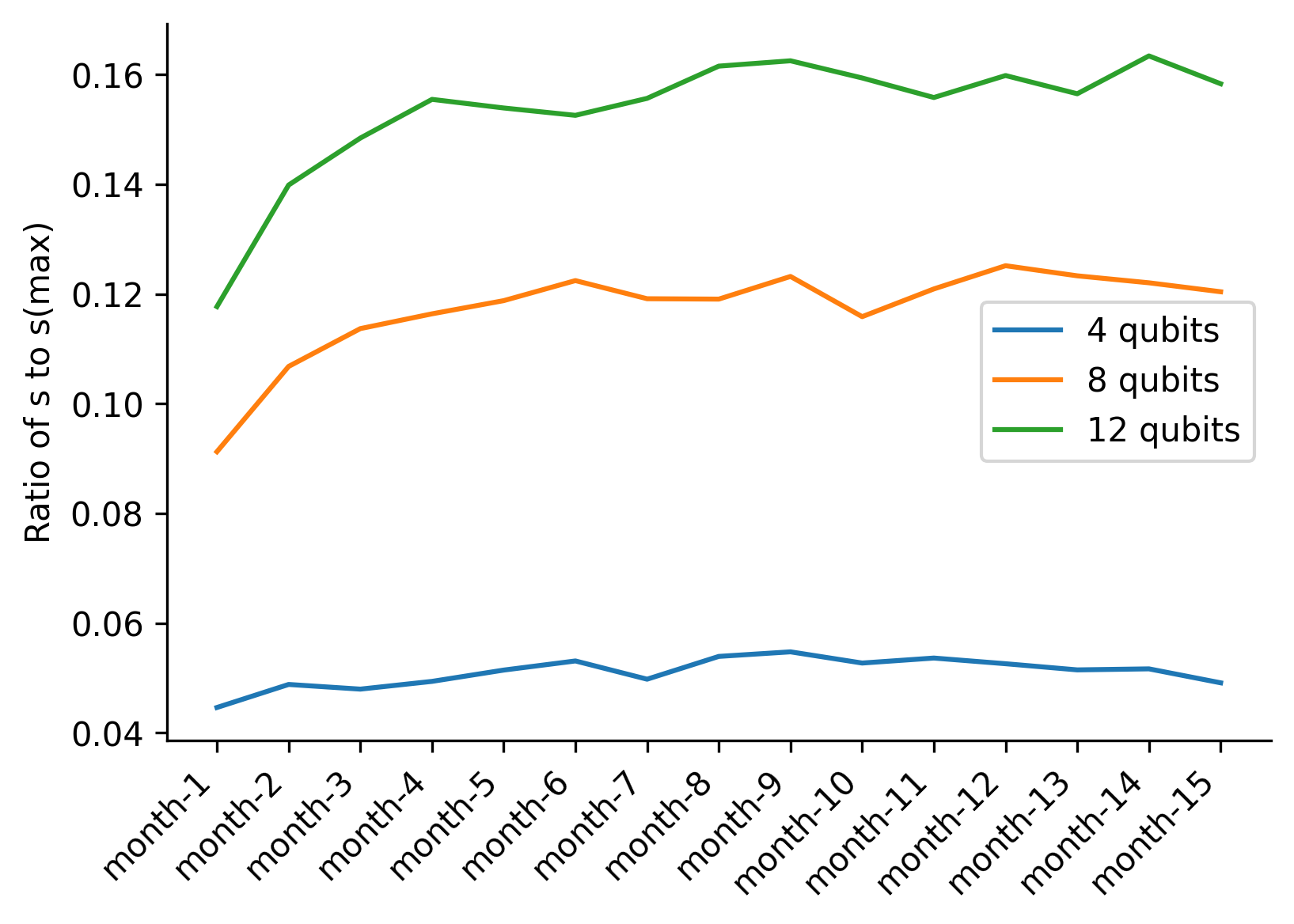
Figure 3. The ratio $s/s_{\textrm{max}}$ for a simulated time-varying noisy circuit is plotted with respect to the increasing noise variance across 15 months. The results from noisy simulations of the Bernstein-Vazirani circuit with a secret string of 4, 8, or 12 bits validate the bound expected by Eqn. 17. Details of the simulation models and methods given in the text.

This figure verifies the reliability bound on $s$ (deviation of the mean observable from a reference time) given by Eqn. 17.

Fig. 3 plots the ratio of the simulated stability $s(t,0)$ to the upper bound $s_{\textrm{max}}$ with respect to the simulated month for the cases of 4, 8, and 12-bit secret-strings; an additional ancilla qubit is required for each circuit implementation. In all cases, the results confirm the bound on the observable stability provided by Eqn. 17 as indicated by the ratio less than unity. We note that increasing the noise variance each month produces an increase in both the observable stability $s$ and the denominator s${}_{\textrm{max}}$ such that their ratio does not grow quickly. Additionally, the ratio of $s$ to $s_{\textrm{max}}$ is higher for higher dimensional Hilbert spaces, as $s$ is more sensitive to changes in the Hilbert space dimension than the denominator. For example, in the 4-qubit problem the ratio ranged from 4% to 5%, while for the 8-qubit problem it varied from 9% to 13%, and for the 12-qubit problem, it ranged from 12% to 16%. These results show that the ratio remains below 1 for these different problem sizes and distributions, which validates the reliability bound derived in Eqn. 17.

As a side note, for the Bernstein-Vazirani circuit in Fig. 2, when the noise parameter distribution is independent, wide-sense stationary and the noise channel is a polynomial of degree $\leq 2$ in the noise parameter x, then $s=|\braket{O}_{t}-\braket{O}_{0}|$ is always 0 as $\braket{O}_{t}$ becomes time-invariant. The depolarizing noise is an example of such a channel where only first-order error terms are present. See Appendix A.2 for details.

3. Testing reliability

Given the aforementioned bounds on statistical similarity, we now consider how reliability of a noisy quantum device can be tested empirically.

3.1. Experimental Data Set

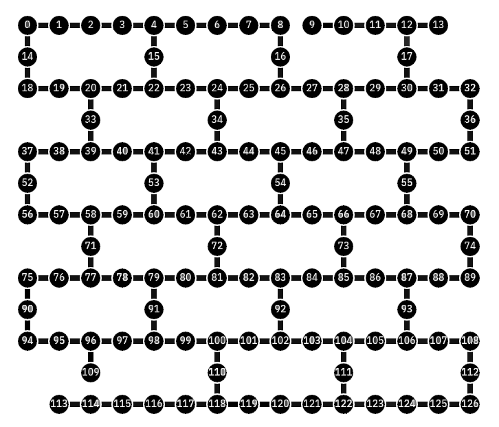
Figure 4. Schematic layout of the $127$-qubit washington device produced by IBM. Circles denote register elements and edges denote connectivity of 2-qubit operations. The register elements $0$, $1$, $2$, $3$, and $4$ in Fig. 9 are mapped to the physical qubits $4$, $3$, $2$, $1$, and $0$, respectively, in the diagram above. The CNOT gates used in the circuit connect the physical qubits $(0,1)$ and $(2,1)$, in the diagram above, where the first number represents the control qubit and the second one represents the target qubit.

Schematic layout of the $127$-qubit washington device produced by IBM. Circles denote register elements and edges denote connectivity of 2-qubit operations. The register elements $0$, $1$, $2$, $3$, and $4$ in Fig. 9 are mapped to the physical qubits $4$, $3$, $2$, $1$, and $0$, respectively, in the diagram above. The CNOT gates used in the circuit connect the physical qubits $(0,1)$ and $(2,1)$, in the diagram above, where the first number represents the control qubit and the second one represents the target qubit.

We investigate the reliability of the washington superconducting transmon device, which is developed by IBM and consists of a $127$-qubit register with heavy hexagonal connectivity. The device encodes information in the lowest lying levels of the coupled transmons, and operations are implemented using shaped microwave pulses to drive gate dynamics (krantz2019quantum, ). Of specific interest for our purposes is that characterization data for the washington device is periodically published publicly and this may be used to create a data set of select device metrics (ibm_quantum_experience_website, ).

We created a data set from a subset of device characterization data for a $16$-month period starting on 1-Jan-2022 and ending on 30-Apr-2023. The following characterization data was collected each day:

1. date and time when device was characterized,

2. average SPAM error rate for each register element,

3. CNOT gate error, obtained using randomized benchmarking from a sequence of two-qubit Clifford gates with different lengths,

4. CNOT gate duration and the unit of measure as, e.g. cx01_gate_length, cx01_gate_length_unit

5. de-coherence time for each register, the unit of measure, and the date and time of the characterization, e.g. q0_T2, q0_T2_unit, and q0_T2_cal_time

The collected characterization data was accessed online using the Qiskit software library (aleksandrowicz2019qiskit, ), and a sample time-series of the data is shown in Fig. 1. The data provides valuable information for assessing the reliability of the washington device and can be used for further analysis and experimental validation of quantum computing applications.

3.2. Experimental Analysis

Parameter	Description
$\textrm{x}_{0}$	SPAM fidelity for register element 0
$\textrm{x}_{1}$	SPAM fidelity for register element 1
$\textrm{x}_{2}$	SPAM fidelity for register element 2
$\textrm{x}_{3}$	SPAM fidelity for register element 3
$\textrm{x}_{4}$	CNOT gate fidelity for control 0, target 1
$\textrm{x}_{5}$	CNOT gate fidelity for control 2, target 1
$\textrm{x}_{6}$	$T_{2}$ de-coherence time for register element 0
$\textrm{x}_{7}$	$T_{2}$ de-coherence time for register element 1
$\textrm{x}_{8}$	$T_{2}$ de-coherence time for register element 2
$\textrm{x}_{9}$	$T_{2}$ de-coherence time for register element 3
$\textrm{x}_{10}$	$T_{2}$ de-coherence time for register element 4
$\textrm{x}_{11}$	Hadamard gate fidelity for register element 0
$\textrm{x}_{12}$	Hadamard gate fidelity for register element 1
$\textrm{x}_{13}$	Hadamard gate fidelity for register element 2
$\textrm{x}_{14}$	Hadamard gate fidelity for register element 3
$\textrm{x}_{15}$	Hadamard gate fidelity for register element 4

Table 2. Device parameters

Device parameters

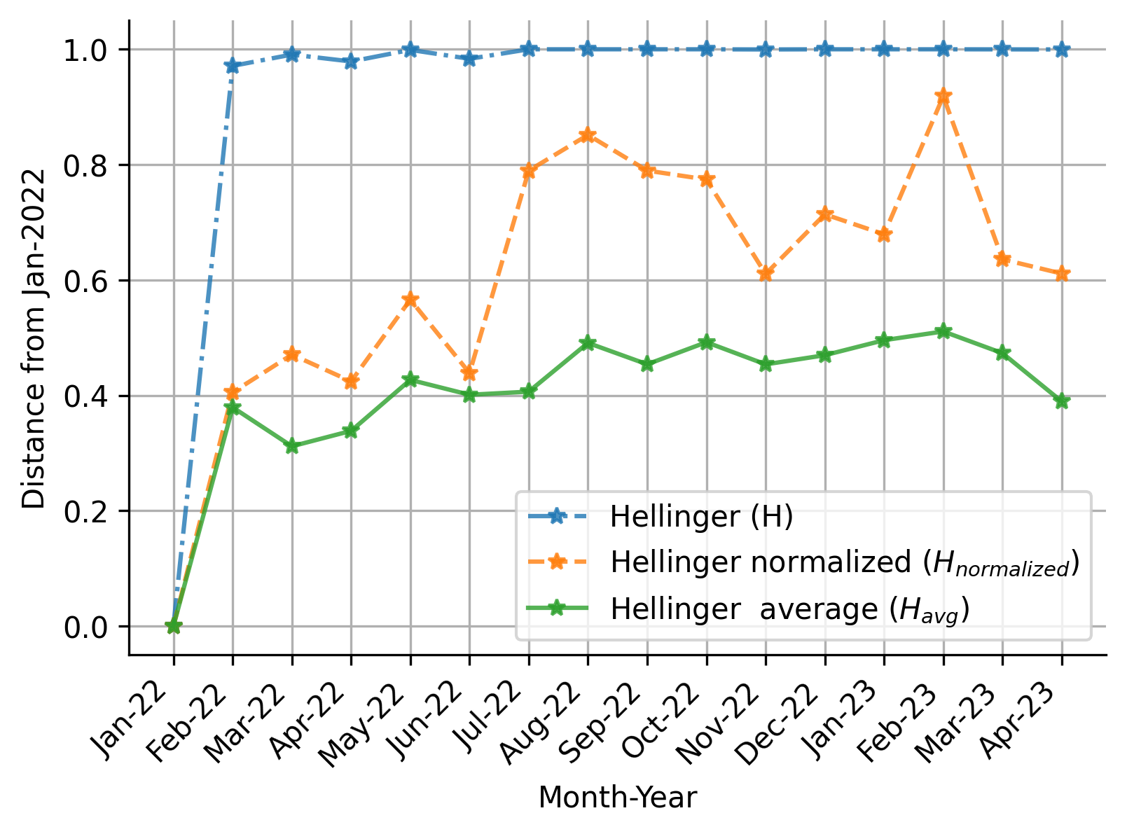
Figure 5. The figure presents results of reliability testing on a transmon platform over 16 months. Plots of the three Hellinger distance measures, with the unmodified measure $H$ (blue line) being insensitive due to dimensionality issues. The blue and orange lines both capture the correlation structure of the joint distribution (with the orange line being normalized to enhance discrimination power), while the green line lacks correlation capture. The normalized measure $H_{\textrm{normalized}}$ ranges between 0.41 and 0.92, while the average measure $H_{\textrm{avg}}$ varies between 0.431 and 0.51. The latter captures monthly variations in the marginal Hellinger distance for each of the 16 error parameters but fails to account for correlations.

The figure presents results of reliability testing on a 127-qubit transmon platform

We next examine the reliability of the device parameters with respect to the SPAM fidelity, gate fidelity, duty cycle, and addressability of 5 qubits, as shown in Table 2. We calculate $H_{X}(t,t_{0})$ for $X=(X_{0},\cdots,X_{15})$ with $t$ in the set of months spanning from Jan-2022 to Apr-2023 and $t_{0}$ set to Jan-2022. For each month, the univariate noise distributions consist of approximately 30 points representing daily measurements. The marginal Hellinger distance for each of the 16 error parameters is reported in Table 3 of the Appendix. We then model the monthly joint distributions from this dataset using the previously discussed methods of copulas.

Fig. 5 plots the results from device reliability for the three different variations of the Hellinger distance. The unmodified Hellinger distance per Eqn. 6, which is less sensitive due to the curse of dimensionality (see the discussion in Section 2.2). The orange line represents the normalized Hellinger distance per Eqn. 11, while the green line represents the Hellinger distance averaged over all the marginal distributions per Eqn. 10. The data range refers to the disparity between the highest and the non-zero lowest values found in the observed dataset. A statistical test that produces data with a larger data range indicates a stronger ability to discriminate. The normalized and average Hellinger distances, represented by the orange and green lines respectively, demonstrate greater discriminatory power with the observed data ranges of 0.51 and 0.20, respectively. These ranges are considerably higher compared to the unmodified Hellinger distance with an observed data range of 0.029.

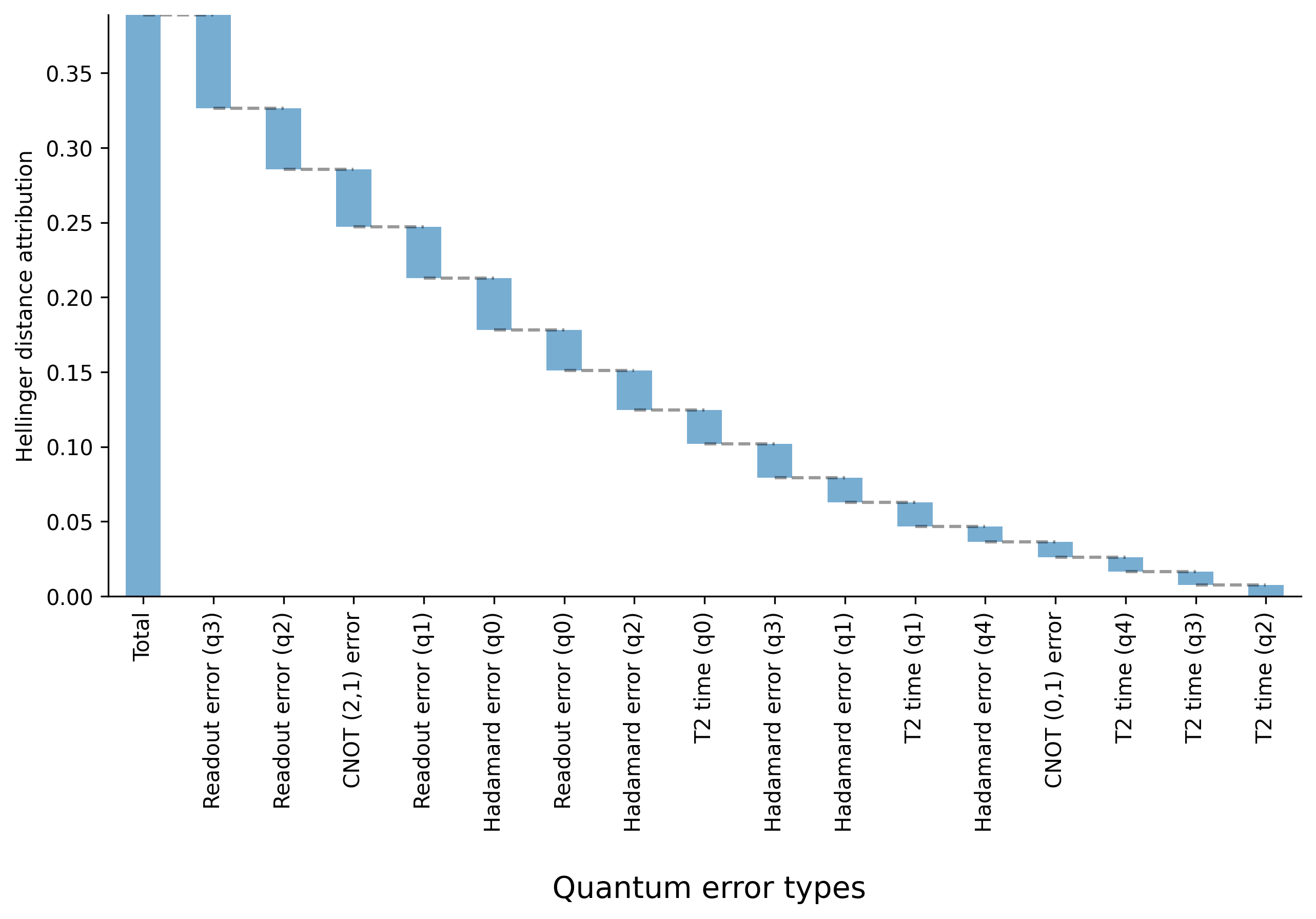
Figure 6. A plot the contributions made by each device metric to the Hellinger distance. The coordinates label the corresponding metric and the ordinates show the average of the Hellinger distance measures. The computed distance compares the distribution in Apr-2023 to Jan-2022. The metrics contribute varying percentages but no single metric dominates the sum.

This empirical plot investigates which metrics for device characterization are responsible for the time variation of a quantum computing platform, rendering it unreliable for physical realization.

The normalized Hellinger distance exhibits a range of values between 0.41 and 0.92, while the average Hellinger distance varies from 0.31 to 0.51. The average measure provides monthly variation information for the marginal Hellinger distance of each of the 16 error parameters, as shown in Table 3 in the Appendix. In Fig. 6, the contributions to the average Hellinger distance for Apr-2023 distribution compared to that of Jan-2022 are compared. It is apparent that no single parameter dominates the average though SPAM error accounts for the largest contribution. It is important to note that the average measure does not consider correlations between parameters, and a specific correlation structure can cause the joint distance to increase by reducing overlap in a subset of dimensions.

4. Computing on unreliable platforms

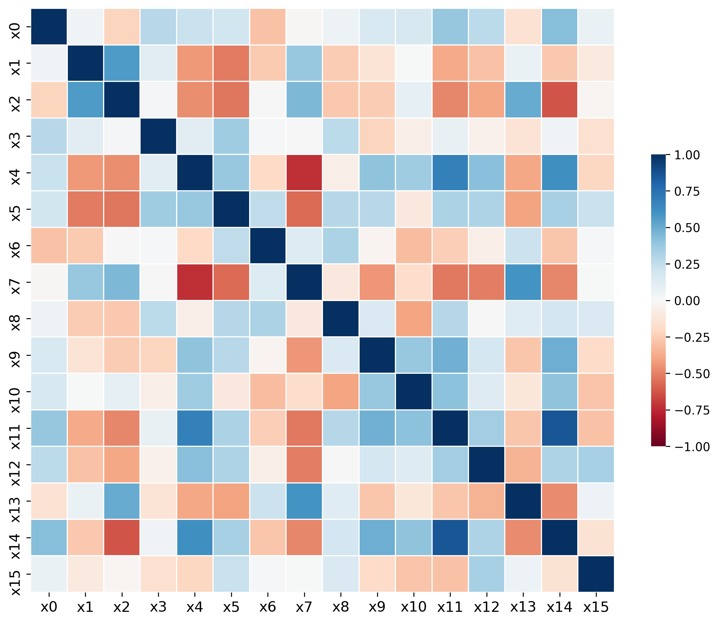
Figure 7. The Pearson coefficients between the 16 characterization parameters defined in Table 2 displayed in matrix format with the axes of corresponding indices. Blue and red colors signify Pearson coefficients between $1$ and $-1$, respectively. The plotted data derives from daily observations made in April-2023.

This figure presents a heatmap of correlations among the 16 circuit .

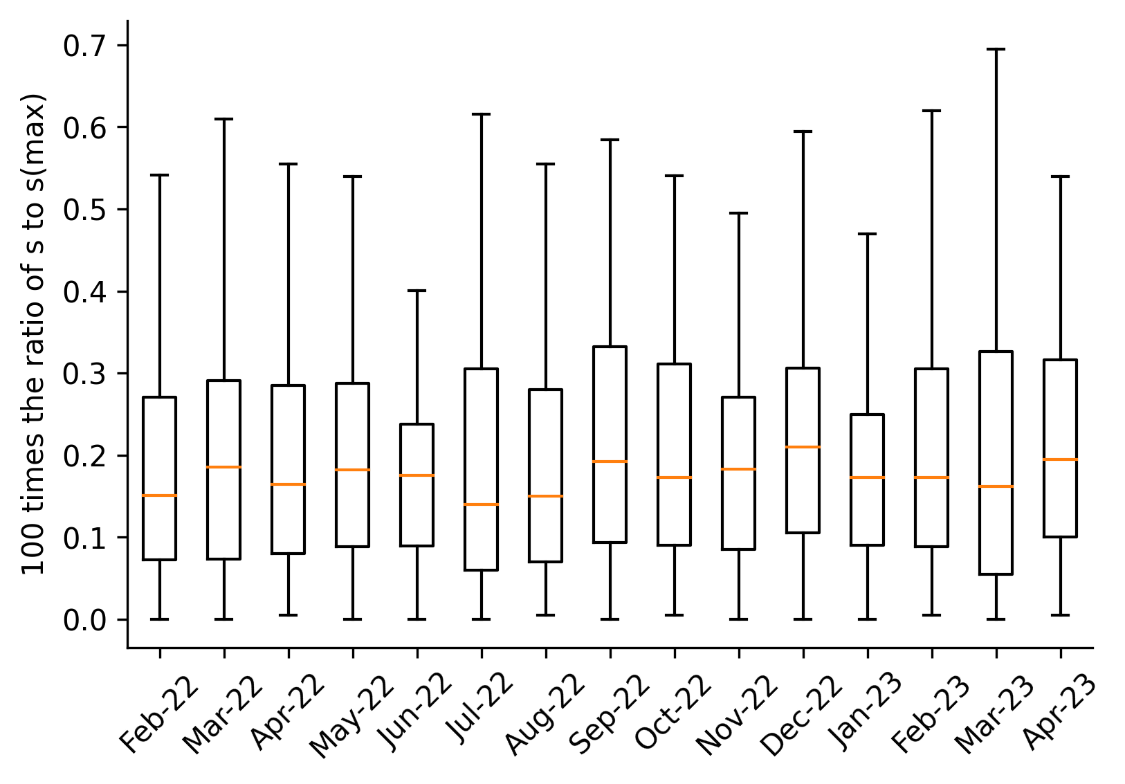
Figure 8. Simulations of the stability ratio $s/s_{max}$ times 100 for a 4-qubit Bernstein-Vazirani circuit using the noise characterization from the IBM washington platform. The box-and-whisker plot of the monthly statistics are based on noisy circuit simulations using the joint probability distribution derived from data from 1-Jan-2022 to 30-Apr-2023. Ratio values below unity confirm that the upper bound from Eqn. 17 is never exceeded.

We implemented a 4-qubit Bernstein-Vazirani circuit on the IBM washington platform and modeled the monthly joint noise distribution (across the 16 circuit parameters).

We now verify the bound on observable stability from Eqn. 17 using the characterization data for the washington device. Our model uses the explicit circuit representation of the Bernstein-Vazirani algorithm shown in Fig. 9 of the Appendix, in which register elements $0$, $1$, $2$, $3$, and $4$ are mapped to the locations $4$, $3$, $2$, $1$, and $0$, respectively, on the physical platform shown in Fig. 4. The CNOT gates used in the circuit connect the physical qubits $(0,1)$ and $(2,1)$, where the first number represents the control qubit and the second one represents the target qubit. We simulate this noisy 4-qubit Bernstein-Vazirani circuit using the characterization data from the washington platform between from 1-Jan-2022 to 30-Apr-2023 to verify the stablity bound is satisfied.

We first explain the methods for reconstructing the probabilistic noise models for the washington device from the monthly characterization data. Fig. 7 shows the correlation between the 16 device parameters taken from Table 2. Axes index the corresponding parameters and the presented results correspond to daily observations made in Apr-2023. The figure presents the Pearson coefficients with blue shades indicative of positive correlation and red shades indicative of negative correlation. For example, the Hadamard error for qubits 0 and 3 exhibits a significant correlation of 0.86. Diagonal elements are set to 1.0 to represent each variable’s correlation with itself. Generally, monthly correlation datasets reveal that daily values of the device parameters are not independent and our estimate for the error bars on these coefficients is approximately $1/\sqrt{30-1}\approx 0.18$.

We constructed the composite probability distribution including these correlations using the copulas method (sklar1959fonctions, ) discussed in Eqn. 30. The full 16-dimensional distribution cannot be visualized but the significance of these correlations is apparent from the example of a bivariate marginal distribution shown in Fig. 10, which compares the constructed probability distribution with and without correlation. Accurate representation of the experimentally observed data distribution necessitates modeling correlations. Importantly, the correlation structure itself changes monthly with the characterization data.

The full 16-dimensional problem requires a high Monte Carlo sampling overhead for convergence as per Eqn. 33. To address this issue, we determined that our machine’s configuration allows for a Monte Carlo sampling size of 100,000, which corresponds to a program runtime of approximately six hours including qiskit simulations and Monte Carlo sampling overhead. Introducing a threshold for correlation enables the clustering of variables and reduces the effective problem dimensionality, thereby resulting in Monte Carlo convergence within the sampling budget. To determine the desired threshold, we ran a loop for the correlation threshold from 1.0 to 0.0 in step sizes of -0.01 for a given maximum cluster size, computing the maximum resultant cluster size across our dataset at each step. Once we hit the desired max cluster size, we break out of the loop and choose that as our threshold (0.78 in our study) for simulation purposes. This thresholding scheme is used solely for computational feasibility purposes, and the resulting cluster set changes monthly as the correlation matrix changes monthly.

As the correlations between device parameters varies each month, the number of clusters and their composition also changes. For example, in May 2022, our methods identified 13 clusters with the biggest cluster comprising 3 device parameters, while in April 2023, we found 16 independent clusters. Generally, given $d$ device parameters that form $K$ independent clusters at time $t$, denote the $i$-th cluster as $\mathcal{B}_{i}(t)$. The cardinality of $\mathcal{B}_{i}(t)$ is denoted by $m_{i}(t)$, such that $\sum_{i}m_{i}(t)=d$ for all $t$. Let the elements of $\mathcal{B}_{i}(t)$ be given by $\{\textrm{x}_{(1,i)},\cdots,\textrm{x}_{(m_{i}(t),i)}\}$ and let $\Theta_{i}(t)$ from Eqn. 30 denote the copula function for cluster $\mathcal{B}_{i}(t)$, i.e.,

(36) $$\Theta_{i}(t)=\Theta\left[F_{X_{(1,i)}}\left(\textrm{x}_{(1,i)};t\right),\cdots,F_{X_{(m_{i}(t),i)}}\left(\textrm{x}_{(m_{i}(t),i)};t\right)\right].$$

Then, Eqn. 33 becomes:

(37) $$1-H^{2}_{X}= \mathds{E}\left(\sqrt{\frac{\underset{i\in t_{1}\textrm{ clusters}}{\prod}\Theta_{i}(t_{2})}{\underset{j\in t_{2}\textrm{ clusters}}{\prod}\Theta_{j}(t_{1})}\prod\limits_{k=1}^{d}\frac{f_{X_{k}}(\textrm{x}_{k};t_{2})}{f_{X_{k}}(\textrm{x}_{k};t_{1})}}\right),$$

which we will approximate through Monte Carlo sampling.

We use 100,000 Markov-Chain Monte Carlo simulations to estimate $\braket{O}_{t}$ for a given month. This sample size was chosen based on numerical convergence by using the Qiskit Aer numerical simulator to calculate noisy simulations of the circuit. From these estimates, we then calculated the monthly average observable value, $\braket{O}_{t}$ and the observable stability, $s=|\braket{O}_{t}-\braket{O}_{0}|$. Moreover, we performed these simulation 100 times for each month to estimate the underlying distribution for the stability itself.

Fig. 8 presents the the observable stability $s$ to s${}_{\textrm{max}}$ ratio from these simulations for each month. In this box-and-whisker plot, the central box at each point signifies the interquartile range (IQR), with its lower and upper edges representing the first (Q1) and third quartiles (Q3), respectively. The median is indicated by a line within the box. Notably, all ratios remain well below unity and verify that the upper bound calculated from characterization data is never surpassed. These results quantitatively bound temporal changes in program execution using characterization data alone.

From Fig. 8, we also see that our upper bound for the temporal variations of the quantum observable is significantly higher than the experimentally observed values. Tighter upper bounds are more useful than looser ones as they allow for more accurate decision-making and avoid unnecessary over-engineering. If the bounds are tighter, they accurately represent the device noise, capturing its true characteristics. On the other hand, looser bounds result in an overestimation of the device noise. Underestimating the noise is not viable as it would no longer serve as a bound. When noise is overestimated, it raises the threshold for required performance improvement as dictated by the bound, leading to an excessive and unnecessary level of engineering. Therefore, tighter bounds offer more flexibility in accommodating platform noise characteristics, while loose bounds impose unnecessarily restrictive requirements. We offer additional comments on how to improve these bounds in the Appendix. Despite not being very tight, our bound in Eqn. 17 is still useful for several reasons. Firstly, it helps estimate the maximum temporal variations and ensures result reproducibility. Secondly, if the platform noise stays within the bounds determined by the analysis, experimental reproducibility can be guaranteed with a high degree of certainty. Finally, numerical simulations using real data allow us to scale down the requirements to be less restrictive.

5. Conclusion

We have shown how fluctuations in device parameters, such as non-ideal gate executions and imperfect isolation systems, are a significant concern for stable and reproducible NISQ computing demonstrations. Current experimental demonstrations often rely on quantum circuits calibrated immediately prior to program execution or tuned during run-time. However, the resulting circuits and device calibrations are implicitly dependent on the device parameters, which fluctuate significantly over time, across the register, and with varying technology. An unreliable quantum device used for computational purposes is not suitable for reproducible error attribution or uncertainty quantification. Our results have shown that reliability is fundamental for the testing and evaluation of NISQ devices and application benchmarks by presenting a bound on program stability relative to variations in the device parameters.

We have further validated these bounds and quantified the reliability of a superconducting transmon architecture by comparing gate fidelities, duty cycles, and register addressability across multiple temporal and spatial scales. We studied distribution similarity of test observables as an indicator of reliability and we analyzed the reliability of a composite quantum computing platform model a well-characterized noise parameters that exhibit time-varying statistics. Finally, we used the Bernstein-Vazirani algorithm as a test circuit and conducted simulations of the behavior using monthly characterization data from the IBM washington device.

Note that Eqn. 17 does not provide a tight bound due to three sources. Firstly, we can make Eqn. 38 tighter by restricting ourselves to scenarios where the noise distribution function at a later time is consistently lower than at an earlier time, which often occurs in between calibrations. In fact, the reason that Fig. 3 was able to achieve a more accurate estimate of the temporal variations of the quantum observable is because we had modeled an in-between calibrations scenario. Secondly, the use of Hölder’s inequality introduces additional loss of tightness, since the equality holds only when the two functions are linearly dependent, which is highly unlikely in our context. Each application of Hölder’s inequality makes the bound looser. Thirdly, Eqn. 41 leads to a looser bound for observables that heavily fluctuate with platform characterization metrics. This approximation, found in the appendix, employs the maximum value of $\braket{O_{\textrm{x}}}$ to set the integral’s bound. The accuracy of this approximation diminishes as $\braket{O_{\textrm{x}}}$ fluctuates more with x, while it improves with less variation in x. In our Bernstein-Vazirani application, where $\braket{O_{\textrm{x}}}$ ranges from 0 to 1, this introduces significant approximation, contributing to the observed loose bound.

The upper bound on the observable stability is directly related to the time-varying noise statistics of the device. Our results suggest that the experimental noise of the washington device change significantly on a monthly time scale. We note that any threshold or tolerance selected for assessing device reliability will be application specific as obtained from the derived bound. For example, if we require that the mean of the observable of the Bernstein-Vazirani circuit at time $t_{2}$ be within $\pm 0.25$ of the output at time $t_{1}$, then the distribution similarity measure $H_{\textrm{normalized}}(t_{1},t_{2})$ needs to be less than 2.2%. However, $H_{\textit{normalized}}$ varied between $0.41$ and $0.92$ over the one-and-a-half year period Jan-2022 to Apr-2023, and this indicates that the device was not reliable for consistently reproducing the statistical mean.

Reliability is a critical feature for testing and evaluating NISQ devices, and our realiablity test should guide improvements in the characteristics and refinement of as well as metadata analysis of the calibration date, optimal pulse data, and other features about device operations. We anticipate these results will impact future studies on the non-stationarity of quantum channels at even shorter time scales and smaller spatial scales and also support the design of protocols for stable benchmarks.

Code and Data

The code and data are for available publicly available in the github repository:
https://github.com/quantumcomputing-lab/nisqReliability

Appendix A Appendix

A.1. Bound on the temporal stability

Let $s(t_{1},t_{2})$ be the absolute difference in the mean of the observable obtained from the execution of the noisy quantum program at times $t_{1}$ and $t_{2}$. Then,

(38) $$s^{2}(t_{1},t_{2}) =\left(\braket{O}_{t_{1}}-\braket{O}_{t_{2}}\right)^{2}$$

$$=\left(\int\braket{O_{\textrm{x}}}f_{X}(\textrm{x};t_{1})\textrm{dx}-\int\braket{O_{\textrm{x}}}f_{X}(\textrm{x};t_{2})\textrm{dx}\right)^{2}$$

$$\leq\left(\int\left|\braket{O_{\textrm{x}}}\{f_{X}(\textrm{x};t_{1})\textrm{dx}-f_{X}(\textrm{x};t_{2})\}\right|\textrm{dx}\right)^{2}.$$

In the last step, the inequality stems from the absolute value on the integrand. Now, per Hölder’s inequality, if $m,n\in[1,\infty)$ and

$$\frac{1}{m}+\frac{1}{n}=1,$$

then:

$$\int\left|f(x)g(x)\right|dx\leq\left(\int|f(x)|^{m}dx\right)^{1/m}\left(\int|g(x)|^{n}dx\right)^{1/n}.$$

Thus, our inequality becomes:

(39) $$\left(\int\left|\braket{O_{\textrm{x}}}\{f_{X}(\textrm{x};t_{1})\textrm{dx}-f_{X}(\textrm{x};t_{2})\}\right|\textrm{dx}\right)^{2}\leq\left[\left(\int|\braket{O_{\textrm{x}}}|^{m}\textrm{dx}\right)^{1/m}\left(\int|f_{X}(\textrm{x};t_{1})-f_{X}(\textrm{x};t_{2})|^{n}\textrm{dx}\right)^{1/n}\right]^{2}.$$

Now, let $m\rightarrow\infty,n=1$ and define:

(40) $$c=\underset{\textrm{x}}{\textrm{sup}}|\braket{O_{\textrm{x}}}|.$$

Clearly,

(41) $$\lim\limits_{m\rightarrow\infty}\left(\int|\braket{O_{\textrm{x}}}|^{m}\textrm{dx}\right)^{1/m}\leq\lim\limits_{m\rightarrow\infty}\left(\int c^{m}\textrm{dx}\right)^{1/m}=c\left(\lim\limits_{m\rightarrow\infty}\left(\int\textrm{dx}\right)^{1/m}\right)=c.$$

Thus, we have

(42) $$s(t_{1},t_{2})^{2} \leq\lim\limits_{m\rightarrow\infty,n=1}\left(\left(\int|\braket{O_{\textrm{x}}}|^{m}\textrm{dx}\right)^{1/m}\left(\int|\{f_{X}(\textrm{x};t_{1})\textrm{dx}-f_{X}(\textrm{x};t_{2})\}|^{n}\textrm{dx}\right)^{1/n}\right)^{2}$$

$$=c^{2}\left(\int\left|\sqrt{f_{X}(\textrm{x};t_{1})}-\sqrt{f_{X}(\textrm{x};t_{2})}\right|\left(\sqrt{f_{X}(\textrm{x};t_{1})}+\sqrt{f_{X}(\textrm{x};t_{2})}\right)\textrm{dx}\right)^{2}$$

$$=c^{2}\int\left(\sqrt{f_{X}(\textrm{x};t_{1})}-\sqrt{f_{X}(\textrm{x};t_{2})}\right)^{2}\textrm{dx}\int\left(\sqrt{f_{X}(\textrm{x};t_{1})}+\sqrt{f_{X}(\textrm{x};t_{2})}\right)^{2}\textrm{dx}\;\;\;\;\textrm{ (applying H\"{o}lder's inequality with m=n=2)}$$

$$=c^{2}\int\left(f_{X}(\textrm{x};t_{1})+f_{X}(\textrm{x};t_{2})-2\sqrt{f_{X}(\textrm{x};t_{1})}\sqrt{f_{X}(\textrm{x};t_{1})}\right)\textrm{dx}\int\left(f_{X}(\textrm{x};t_{1})+f_{X}(\textrm{x};t_{2})+2\sqrt{f_{X}(\textrm{x};t_{1})}\sqrt{f_{X}(\textrm{x};t_{1})}\right)\textrm{dx}$$

$$=c^{2}\left(1+1-2\int\sqrt{f_{X}(\textrm{x};t_{1})}\sqrt{f_{X}(\textrm{x};t_{1})}\textrm{dx}\right)\left(1+1+2\int\sqrt{f_{X}(\textrm{x};t_{1})}\sqrt{f_{X}(\textrm{x};t_{1})}\textrm{dx}\right)$$

$$=4c^{2}H_{X}^{2}(2-H_{X}^{2}),$$

where, for notational clarity, we use:

$$H_{X}^{2}=H^{2}_{X}(t_{1},t_{2})=1-\int\sqrt{f_{X}(\textrm{x};t_{1})}\sqrt{f_{X}(\textrm{x};t_{2})}dx$$

Equation (17) upper bounds temporal variations in the expected mean of the circuit outcome with respect to the statistical reliability of the device metrics. As expected, the temporal variations vanish when $H_{X}=0$ and become maximal when $H_{X}=1$. The bound itself is monotonic with the greatest change occurring for the greatest distance. Note that $c=\underset{\textrm{x}}{\textrm{sup}}|\braket{O_{\textrm{x}}}|$ has no dependence on the time-varying distribution $f_{X}(x;t)$ but it does depend on the noise parametrization for the circuit. Thus the observable stability $s$ is always upper bounded by

$$s^{2}_{\textrm{max}}=4c^{2}H_{X}^{2}(2-H_{X}^{2}),$$

an upper bound determined by the degree of time-variation of the device parameters. Thus,

(43) $$\begin{split}\frac{s}{s_{\textrm{max}}}&\leq 1.\end{split}$$

A.2. Time-invariance for wide-sense stationary noise processes

For the Bernstein-Vazirani problem, $\braket{O}_{t}$ is time-invariant if the noise is independent and wide-sense stationary (WSS) and the quantum channel, as a function of the noise parameter x, is a first-order polynomial (e.g. depolarizing channel). This is because:

(44) $$\begin{split}\braket{O}_{t}=&\int\braket{O_{X}}f_{X}(\textrm{x};t)d\textrm{x}\\ =&\prod_{i=1}^{n}\int\bra{r_{i}}\mathcal{E}_{\textrm{x}_{i}}(\ket{r_{i}}\bra{r_{i}})\ket{r_{i}}f_{X_{i}}(\textrm{x}_{i};t)d\textrm{x}_{i}\\ =&\prod_{i=1}^{n}\int\textrm{(A first-order polynomial in $x_{i}$)}f_{X_{i}}(\textrm{x}_{i};t)d\textrm{x}_{i},\end{split}$$

which is time-invariant because of the wide-sense stationarity assumption, which states that WSS (wide-sense stationary) random processes possess a constant first-order moment and auto-covariance. Thus,

(45) $$s=|\braket{O}_{t}-\braket{O}_{0}|=0\;\;\;\;\forall t.$$

A.3. Curse of dimensionality

Consider $d$ independent and identically distributed circuit error parameters $\{\textrm{x}_{1},\cdots,\textrm{x}_{d}\}$, whose marginal (uni-variate) distributions are given by $f_{X_{i}}(\textrm{x};t)$. Let $h$ be the Hellinger distance between the marginals at time $t_{1}$ and $t_{2}$. Thus,

$$H_{X_{i}}(t_{1},t_{2})=h\;\;\;\;\forall i$$

Since the parameters are independent:

(46) $$\begin{split}\log\left(1-H_{X}^{2}\right)&=-d|\log(1-h^{2})|\\ \Rightarrow H_{X}&=\sqrt{1-\exp\left[-d|\log(1-h^{2})|\right]}.\end{split}$$

Thus the distance approach $1$ quickly as the number of dimensions increases.

A.4. Additional Data

Table 3 displays Hellinger distance values for the device parameters in the context of device reliability testing. The distance is between two time-varying marginal distributions, with the first distribution estimated using data for Jan-2022 as a constant reference. The second distribution is observed at a subsequent time, estimated using data for a specific month between Jan 2022 and Apr 2023. The first 16 columns present Hellinger distance data for time-varying marginal distributions, while the last three columns contain the same for joint distributions. The $H_{r}$ column shows the Hellinger distance between the joint distributions, $H_{a}$ represents the average Hellinger distance over the marginals, and $H_{n}$ represents the normalized Hellinger distance. Detailed definitions for these terms can be found in the main text.

Month	$H_{X_{0}}$	$H_{X_{1}}$	$H_{X_{2}}$	$H_{X_{3}}$	$H_{X_{4}}$	$H_{X_{5}}$	$H_{X_{6}}$	$H_{X_{7}}$	$H_{X_{8}}$	$H_{X_{9}}$	$H_{X_{10}}$	$H_{X_{11}}$	$H_{X_{12}}$	$H_{X_{13}}$	$H_{X_{14}}$	$H_{X_{15}}$	$H_{\textrm{n}}$	$H_{\textrm{a}}$	$H_{\textrm{r}}$
Jan-22	0.0	0.0	0.0	0.0	0.0	0.0	0.0	0.0	0.0	0.0	0.0	0.0	0.0	0.0	0.0	0.0	0.0	0.0	0.0
Feb-22	0.82	0.08	0.43	0.38	0.3	0.35	0.28	0.43	0.45	0.39	0.32	0.24	0.62	0.66	0.04	0.26	0.41	0.38	0.971439
Mar-22	0.97	0.22	0.31	0.3	0.07	0.05	0.31	0.17	0.6	0.22	0.32	0.31	0.11	0.36	0.48	0.17	0.47	0.31	0.99084
Apr-22	0.64	0.03	0.23	0.53	0.27	0.45	0.21	0.06	0.95	0.11	0.1	0.45	0.33	0.37	0.07	0.61	0.42	0.34	0.978632
May-22	0.8	0.27	0.61	0.77	0.11	0.4	0.64	0.21	0.38	0.36	0.26	0.65	0.21	0.34	0.34	0.49	0.57	0.43	0.99897
Jun-22	0.81	0.4	0.43	0.9	0.26	0.34	0.53	0.34	0.28	0.1	0.16	0.36	0.43	0.69	0.16	0.23	0.44	0.4	0.983197
Jul-22	0.74	0.42	0.96	1.0	0.3	0.44	0.15	0.25	0.48	0.37	0.2	0.16	0.38	0.17	0.14	0.32	0.79	0.41	1.0
Aug-22	0.89	0.5	0.9	1.0	0.26	0.41	0.53	0.35	0.97	0.31	0.21	0.55	0.22	0.21	0.27	0.3	0.85	0.49	1.0
Sep-22	0.82	0.48	0.93	1.0	0.45	0.22	0.44	0.34	0.91	0.1	0.08	0.46	0.27	0.31	0.31	0.13	0.79	0.45	1.0
Oct-22	0.72	0.55	0.9	1.0	0.05	0.42	0.32	0.18	0.95	0.07	0.27	0.43	0.36	0.66	0.74	0.25	0.77	0.49	1.0
Nov-22	0.36	0.63	0.65	1.0	0.4	0.13	0.55	0.53	0.98	0.22	0.14	0.4	0.29	0.39	0.29	0.3	0.61	0.45	0.999713
Dec-22	0.42	0.64	0.58	1.0	0.27	0.53	0.45	0.24	0.99	0.17	0.27	0.7	0.65	0.03	0.19	0.37	0.72	0.47	0.999995
Jan-23	0.46	0.59	0.46	1.0	0.06	0.5	0.31	0.3	0.91	0.53	0.26	0.69	0.55	0.34	0.53	0.46	0.68	0.5	0.999975
Feb-23	0.45	0.61	0.65	1.0	0.44	0.46	0.44	0.26	1.0	0.12	0.52	0.53	0.4	0.33	0.61	0.34	0.92	0.51	1.0
Mar-23	0.47	0.5	0.79	1.0	0.22	0.21	0.46	0.33	0.51	0.21	0.4	0.71	0.62	0.09	0.71	0.31	0.64	0.47	0.999876
Apr-23	0.43	0.55	0.65	1.0	0.16	0.61	0.37	0.25	0.12	0.14	0.15	0.55	0.26	0.42	0.36	0.17	0.61	0.39	0.999721

Table 3. Hellinger distance values for the device parameters.

This table displays Hellinger distance values for the device parameters.

Fig. 9 displays the Bernstein-Vazirani circuit, designed for a 4-bit secret string $r=0011$. Real noise data for the washington device was collected using the qiskit software suite. The boxes labeled with $H$ represent the Hadamard gates. The boxes labeled with $Z$ represent the Z gates, which apply a phase shift of $180$ degrees to the $\ket{1}$ state. The meter symbols represent the measurement operation, which measures the qubit in the computational basis and records the result in a classical register.

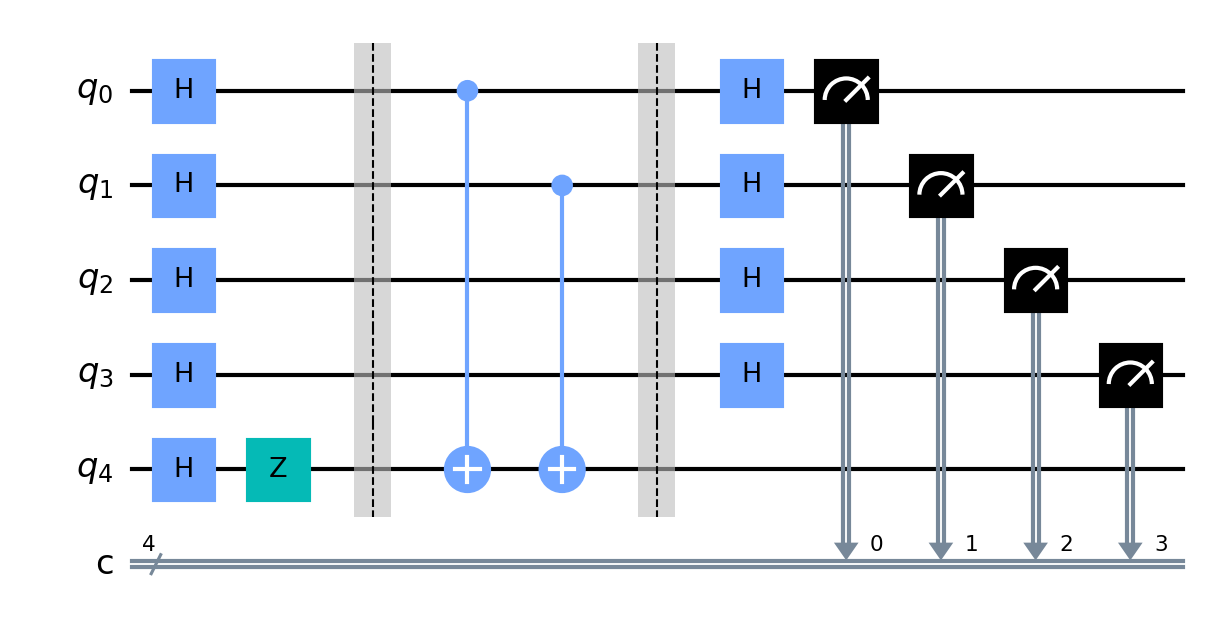
Figure 9. Bernstein-Vazirani circuit, designed for a 4-bit secret string $r=0011$.

This plot displays the schematic of the Bernstein-Vazirani circuit, designed for a 4-bit secret string $r=0011$ on an IBM transmon platform. Real noise data for the IBM Washington device, which exhibits time-varying noise characteristics, is collected using the qiskit Aer simulation suite.

Fig. 10 helps us to visualize a two-dimensional subset of the Hadamard gate errors for qubit 0 and 3, which display an 86% correlation. We use a contour plot to compare the probability density for Apr-2023 (a) with and (b) without correlation modeling using a copula function. The y-axis represents Hadamard gate error for qubit 3, while the x-axis represents the same for qubit 0. Figure (a) shows an angularly tilted ellipse due to 86% correlation, while figure (b) shows symmetric concentric circles due to zero correlation. The presence of correlations can significantly change the overlap between the distributions at different times.

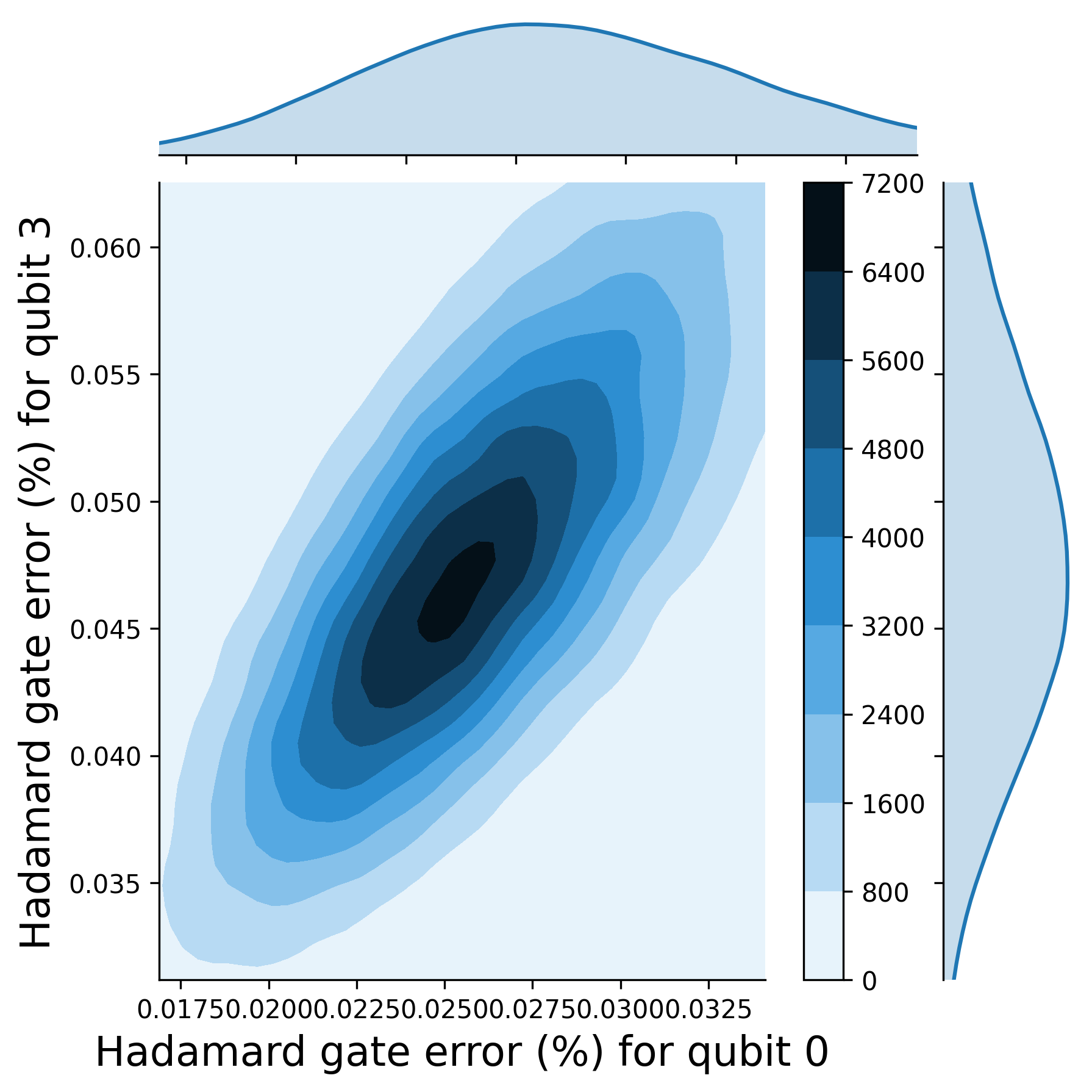
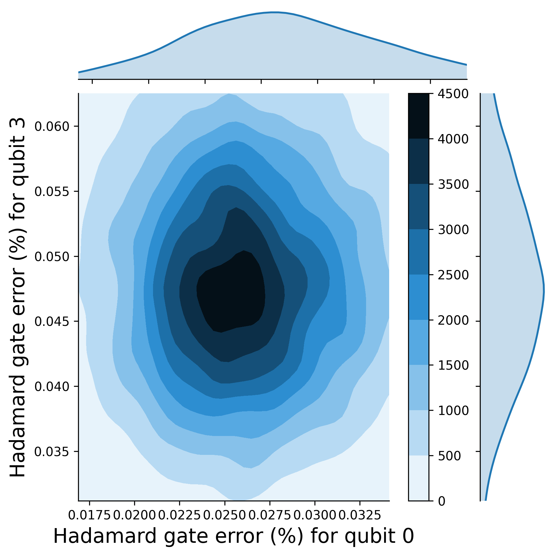
(a)	(b)

Figure 10. Contour plots to compare the probability densities of a two-dimensional subset of Hadamard gate errors for qubit 0 and 3 in Apr-2023, (a) with and (b) without correlation modeling using a copula function.

This graph highlights the importance of correlation modeling for characterizing joint noise distributions for device characterization metrics.