Anti-de Sitterian “massive” elementary systems
and their Minkowskian and Newtonian limits

Abstract

We elaborate the definition and properties of “massive” elementary systems in the $(1+3)$-dimensional Anti-de Sitter (AdS₄) spacetime, on both classical and quantum levels. We fully exploit the symmetry group Sp$(4,{\mathbb{R}})$, that is, the two-fold covering of SO${}_{0}(2,3)$ (Sp$(4,{\mathbb{R}})\sim$ SO${}_{0}(2,3)\times{\mathbb{Z}}_{2}$), recognized as the relativity/kinematical group of motions in AdS₄ spacetime. In particular, we discuss that the group coset Sp$(4,{\mathbb{R}})/\mathrm{S}\big{(}\mathrm{U}(1)\times\mathrm{SU}(2)\big{)}$, as one of the Cartan classical domains, can be interpreted as a phase space for the set of free motions of a test massive particle on AdS₄ spacetime; technically, in order to facilitate the computations, the whole process is carried out in terms of complex quaternions. The (projective) unitary irreducible representations (UIRs) of the Sp$(4,{\mathbb{R}})$ group, describing the quantum version of such motions, are found in the discrete series of the Sp$(4,{\mathbb{R}})$ UIRs. We also describe the null-curvature (Poincaré) and non-relativistic (Newton-Hooke) contraction limits of such systems, on both classical and quantum levels. On this basis, we unveil the dual nature of “massive” elementary systems living in AdS₄ spacetime, as each being a combination of a Minkowskian-like massive elementary system with an isotropic harmonic oscillator arising from the AdS₄ curvature and viewed as a Newton-Hooke elementary system. This matter-vibration duality will take its whole importance in the quantum regime (in the context of the validity of the equipartition theorem) in view of its possible rôle in the explanation of the current existence of dark matter.

I Introduction

For a physical system, like a “free” elementary system living in (A)dS₄ spacetime de Sitter , for which the global and local symmetries of its classical phase space are respectively given by a Lie group $G$ and its Lie algebra $\mathfrak{g}$, the phase space can be naturally identified with an orbit under the co-adjoint action of $G$ in the dual linear space to $\mathfrak{g}$ (denoted here by $\mathfrak{g}^{\circledast}$); such orbits (simply, say co-adjoint orbits) are symplectic manifolds so that each of them carries a natural $G$-invariant (Liouville) measure, and is a homogeneous space homeomorphic to an even-dimensional group coset $G/{\cal{S}}$, where ${\cal{S}}$, being a (closed) subgroup of $G$, stabilizes some orbit point Kirillov1 ; Kirillov2 . On the other hand, co-adjoint orbits, enjoying very rich analytic structures, underlie (projective) Hilbert spaces carrying UIRs of the respective symmetry group, here referred to as $G$. In the sense that was first brought up by Wigner Wigner ; Newton/Wigner in the context of Einstein-Poincaré relativity and then developed by Inönü Wigner1952 , Lévy-Leblond Levy-Leblond , and Voisin Voisin to Galilean systems, and by Gürsey Gursey1963 and Fronsdal Fronsdal 1 ; Fronsdal 2 respectively to dS₄ and AdS₄ systems, the (projective) Hilbert spaces identify (in some restricted sense) the corresponding quantum (“one-particle”) states spaces of the given systems with the symmetry $G$; then, the invariant parameters labeling the (projective) UIRs would represent the basic quantum numbers labeling the states of the respective physical systems. Note that, in such a formulation, a “smooth” transition from classical physics to quantum physics is guaranteed by construction.

In the above sense, we intend in this paper to elaborate the definition and properties of elementary systems in AdS₄ spacetime, on both classical and quantum levels. This work is indeed the natural continuation of a previous article olmogaz19 by del Olmo and Gazeau, which was devoted to such a study in the $(1+1)$-dimensional Anti-de Sitter (AdS₂) spacetime. In a broader picture, however, these two papers are both parts of a series of books/papers serving a wider research plan (see Ref. Gazeau2022 and references therein) that attempts to develop a consistent formulation (in both classical and quantum senses) of elementary systems in the global structure of dS₄ and AdS₄ spacetimes, or in other words, to depict (A)dS₄ relativity versus Einstein-Poincaré relativity. The main motive lying behind this attempt originates from a set of conceptual considerations/worries that we now briefly explain.

First of all, one must notice that both field theoretical formulation and phenomenological treatment of an elementary system, on the level of interpretation in particular, rest on the concepts of energy, momentum, mass, and spin, whose existence is due to invariance principles, strictly speaking, the principle of invariance under the Poincaré group (the relativity group of flat Minkowski spacetime); the rest mass $m$ and the spin $s$ of an (Einsteinian) elementary system living in flat Minkowski spacetime are the two invariants that specify the respective UIR of the Poincaré group Wigner ; Newton/Wigner .

In a curved spacetime, however, any interpretation with reference to the relativity group of flat Minkowski spacetime is physically irrelevant. On the other hand, in curved spacetimes generally (with the exception of dS₄ and AdS₄ spacetimes), no non-trivial groups of motion, and consequently, no literal or unique extension of the aforementioned physical concepts exists. Therefore, although, one may simply generalize the important differential equations (such as Klein-Gordon and Dirac equations) to forms that enjoy general covariance in curved spacetimes, in the end such mathematical constructions cannot be associated with physical elementary systems in the sense given in the previous paragraph.

Nevertheless, the dS₄ and AdS₄ cases constitute a particular family of curved spacetimes, in which the path to generalizations of the aforementioned concepts is well marked, in the sense given by Fronsdal Fronsdal 1 : “A physical theory that treats spacetime as Minkowskian flat must be obtainable as a well-defined limit of a more general physical theory, for which the assumption of flatness is not essential”. The dS₄ and AdS₄ are indeed the two curved spacetimes of constant curvature (respectively, of negative and positive curvatures), which like Minkowski (zero curvature) spacetime, admit continuous groups of motion of maximal symmetry such that, as Minkowski spacetime is the zero-curvature limit of dS₄ and AdS₄ spacetimes, the Poincaré group can be realized by a contraction limit of either the dS₄ relativity group SO${}_{0}(1,4)$ or the AdS₄ one SO${}_{0}(2,3)$. On the representation level, and quite similar to the Poincaré case, the (A)dS₄ UIR’s are labelled by two invariant parameters of the spin and energy scales (the latter, in the AdS₄ case, is actually the rest energy) evans67 ; fronsdal74 ; baelgagi92 ; Gazeau2022 ; Dobrev1 ; Dobrev2 ; 1Thomas ; 2Newton ; 3Takahashi ; 4Dixmier . From the point of view of a local (“tangent”) Minkowskian observer, the (A)dS₄ UIRs fall basically into three sets: the set of (A)dS₄ “massive” UIRs, in the sense that they contract to the Poincaré massive UIRs and exhaust the whole set of the latter evans67 ; 5Mickelsson ; 6Garidi ; the set of (A)dS₄ “massless” UIRs constituting by those (A)dS₄ UIRs with a unique extension to the conformal group (SO${}_{0}(2,4)$) UIRs, while that extension is equivalent to the conformal extension of the Poincaré massless UIRs (of course, this correspondence exhaust the whole set of the Poincaré massless UIRs) 7Barut ; 8Mack ; 9Angelopoulos ; and finally, the set of those (A)dS₄ UIRs with either no physical Poincaré contraction limit or no Poincaré contraction limit at all.

Considering the above and following our goal of developing the relativity of (A)dS₄, we here invoke the Sp$(4,{\mathbb{R}})$ group, which is the two-fold covering of SO${}_{0}(2,3)$ and can also be interpreted as the kinematical/relativity group for AdS₄ spacetime. We first, in section II, present all needed material about AdS₄ spacetime and its relativity group Sp$(4,{\mathbb{R}})$. We also elaborate the geometry of the domain $\mathcal{D}^{(3)}$, that is, a Sp$(4,{\mathbb{R}})$ left coset issued from the Cartan decomposition of the group, with the group action on it in the usual manner; $\mathcal{D}^{(3)}\sim\mathrm{Sp}(4,{\mathbb{R}})/\mathrm{S}(\mathrm{U}(2)\times\mathrm{U}(1))$. This discussion is complemented by studying the Kählerian structure of the Cartan domain $\mathcal{D}^{(3)}$. Then, in section III, we show that this domain can be viewed as the phase space for the set of free motions of a test massive particle living in AdS₄ spacetime. The identification of the ten basic (classical) observables with the Sp$(4,{\mathbb{R}})$ generators and of course the Poincaré and the Newton-Hooke contraction limits of this AdS₄ phase-space structure are given. In section IV, we introduce the discrete series (in a wide sense) of the Sp$(4,{\mathbb{R}})$ representations which act on the Fock-Bargmann Hilbert spaces of holomorphic functions in the Cartan domain $\mathcal{D}^{(3)}$. The corresponding infinitesimal generators, as first-order differential operators acting on the holomorphic functions in $\mathcal{D}^{(3)}$, are also presented. On the quantum level, the Poincaré and the Newton-Hooke contraction limits of the representations are discussed as well. Our results reveal the dual nature of any “massive” elementary system in AdS₄ as a combination of a Minkowskian-like massive elementary system with an isotropic harmonic oscillator due to the curvature and viewed as a Newtonian elementary system. Finally, we summarize our results in section VI. A reminder of the Poincaré and Newton-Hooke groups and their respective UIRs, relevant to the present work, is given in Appendices A and B. Further technical details of the presented mathematical material are also developed in the other appendices.

II AdS₄ spacetime and its relativity group

AdS₄ spacetime is the unique maximally symmetric solution to the vacuum Einstein’s equations with negative cosmological constant $\Lambda$. This constant is linked to the (constant) Ricci curvature $4\Lambda$ of this spacetime. In this context, usually three equivalent fundamental/universal concepts are taken into account in the literature: a fundamental length $\ell_{\Lambda}\equiv\sqrt{3/|\Lambda|}$; a universal frequency $\omega_{\Lambda}=c/\ell_{\Lambda}$ ($c$ being the speed of light); and finally, a universal positive curvature $\varkappa=\sqrt{|\Lambda|/3}$. The most convenient way to visualize the AdS₄ manifold is to embed it in ${\mathbb{R}}^{2,3}$. It then appears as the pseudo-sphere:

$$\mathrm{AdS}_{4}\equiv\Big{\{}y=(y^{\alpha})\in{\mathbb{R}}^{2,3}\;;\;(y)^{2}\equiv\eta_{\alpha\beta}y^{\alpha}y^{\beta} = (y^{5})^{2}+(y^{0})^{2}-(y^{1})^{2}-(y^{2})^{2}-(y^{3})^{2}$$ (II.1)

$$= (y^{5})^{2}+(y^{0})^{2}-\|\boldsymbol{y}\|^{2}={\varkappa}^{-2}\Big{\}}\,,$$

where $\eta_{\alpha\beta}=\mathrm{diag}(+1,+1,-1,-1,-1)$ and the indices $\alpha,\beta,\dotsc$ run on the values $\{5,0,1,2,3\}$. [The number ‘$4$’ is traditionally left out for possible extensions towards conformal theories.] Note that: (i) The embedding Eq. (II.1) makes manifest the O$(2,3)$ symmetry group of AdS₄ spacetime. (ii) The AdS₄ metric is the induced metric from that of flat Minkowski spacetime on the embedding space. In this way, several systems of coordinates can be defined on the AdS₄ manifold. For instance, AdS₄ can be (almost) described by the global coordinates $\{x^{\mu}\}$, which are tensorial with respect to the Minkowski metric $\eta_{\mu\nu}=\mathrm{diag}(+1,-1,-1,-1)$:

$$y^{5} = \left({\varkappa}^{-2}+\|\boldsymbol{x}\|^{2}\right)^{1/2}\cos{\varkappa}x^{0}\,,\quad\quad-\pi\leqslant{\varkappa}x^{0}<\pi\,,$$ (II.2)

$$y^{0} = \left({\varkappa}^{-2}+\|\boldsymbol{x}\|^{2}\right)^{1/2}\sin{\varkappa}x^{0}\,,$$ (II.3)

$$\boldsymbol{y} = (y^{i})=(x^{i})=\boldsymbol{x}\,,\quad\quad x^{i}\in{\mathbb{R}}\,.$$ (II.4)

Another system of coordinates, which will be useful for the sequel, is obtained by a combination of hyperbolic and spherical coordinates:

$$y^{5} = {\varkappa}^{-1}\cosh\varrho\,\cos\theta\,,\quad\quad\varrho\in{\mathbb{R}}^{+}\,,\;-\pi\leqslant\theta<\pi\,,$$ (II.5)

$$y^{0} = {\varkappa}^{-1}\cosh\varrho\,\sin\theta\,,$$ (II.6)

$$\boldsymbol{y} = {\varkappa}^{-1}\sinh\varrho\,\hat{\boldsymbol{y}}\,,\quad\quad\hat{\boldsymbol{y}}\in\mathbb{S}^{2}\,,$$ (II.7)

where $\mathbb{S}^{2}$ is the $2$-sphere.

The relativity/kinematical group of AdS₄ spacetime is SO${}_{0}(2,3)$, that is, the connected subgroup of the identity of the symmetry group O$(2,3)$. The two-fold covering of the SO${}_{0}(2,3)$ group is the real symplectic group Sp$(4,{\mathbb{R}})$ helgason78 . Below, we will study the homomorphism between these two groups. But, before that, let us give a brief outline on complex quaternions, which become handy when we delve more deeply into the mathematical details in the coming discussions.

II.1 Complex quaternions

Note that most of the material and condensed complex quaternionic notations, that are discussed here, are borrowed from Ref. baelgagi92 .

A complex quaternion $z\;\big{(}z\in\mathbb{H}_{\mathbb{C}}\big{)}$ is the scalar-vector pair $(z^{4},\boldsymbol{z})$ written as:

$$z=(z^{4},\boldsymbol{z})\equiv z^{4}+z^{1}\boldsymbol{e}_{1}+z^{2}\boldsymbol{e}_{2}+z^{3}\boldsymbol{e}_{3}\,,$$ (II.8)

where $\left(z^{1},z^{2},z^{3},z^{4}\right)\in{\mathbb{C}}^{4}$, and $\{\boldsymbol{e}_{1},\boldsymbol{e}_{2},\boldsymbol{e}_{3}\}$ satisfy the quaternionic algebra:

$$\boldsymbol{e}_{i}^{2}=-1\,,\quad\boldsymbol{e}_{i}\,\boldsymbol{e}_{j}=\epsilon_{ij}^{\,\,\,k}\boldsymbol{e}_{k}\,,$$ (II.9)

where $\epsilon_{ij}^{\,\,\,k}$ is the three-dimensional totally antisymmetric Levi-Civita symbol. [Note that above we have employed the abusive identification $1\equiv(1,\boldsymbol{0})$.] In the sequel, we denote as well $z^{4}$ by $(z)_{\mathrm{s}}$ (‘$\mathrm{s}$’ for scalar), and also make use of the decomposition of $z$ into real and imaginary parts, i.e., $z=x+\mathrm{i}y$, while $x$ and $y$ are real quaternions ($x,y\in\mathbb{H}$). The complex conjugate, the quaternionic conjugate, and the adjoint of $z$ are respectively defined by:

$$\overline{z}=\left(\overline{z^{4}},\overline{\boldsymbol{z}}\right)\,,\quad\widetilde{z}=(z^{4},-\boldsymbol{z})\,,\quad z^{\ast}=\overline{\widetilde{z}}=\widetilde{\overline{z}}=\left(\overline{z^{4}},-\overline{\boldsymbol{z}}\right)\,,$$ (II.10)

or equivalently by:

$$\overline{z}=x-\mathrm{i}y\,,\quad\widetilde{z}=\widetilde{x}+\mathrm{i}\widetilde{y}\,,\quad z^{\ast}=\widetilde{x}-\mathrm{i}\widetilde{y}\,.$$ (II.11)

The product of two complex quaternions is given by:

$$zz^{\prime}=(z^{4},\boldsymbol{z})({z^{\prime}}^{4},\boldsymbol{z}^{\prime})=\left(z^{4}{z^{\prime}}^{4}-\boldsymbol{z}\cdot\boldsymbol{z}^{\prime},z^{4}\boldsymbol{z}^{\prime}+{z^{\prime}}^{4}\boldsymbol{z}+\boldsymbol{z}\times\boldsymbol{z}^{\prime}\right)\,,$$ (II.12)

where $\boldsymbol{z}\cdot\boldsymbol{z}^{\prime}$ and $\boldsymbol{z}\times\boldsymbol{z}^{\prime}$ are the analytic continuations of respectively the Euclidean inner product and the cross product in ${\mathbb{R}}^{3}$. Note that $\overline{{zz^{\prime}}}=\overline{z}\,\overline{{z^{\prime}}}$ and $\widetilde{{zz^{\prime}}}=\widetilde{{z^{\prime}}}\widetilde{z}$, and hence, $({zz^{\prime}})^{\ast}={z^{\prime\ast}}z^{\ast}$. The determinant of a complex quaternion $z$ is defined by the complex scalar:

$$\det z=\det\widetilde{z}=z\widetilde{z}=\widetilde{z}z=(z^{1})^{2}+(z^{2})^{2}+(z^{3})^{2}+(z^{4})^{2}=\|x\|^{2}-\|y\|^{2}+2\mathrm{i}x\cdot y\,,$$ (II.13)

where $\|x\|^{2}=x\cdot x$ and ‘$\cdot$’ is the Euclidean inner product in ${\mathbb{R}}^{4}\sim\mathbb{H}$. From Eq. (II.13), one derives the expression of the inverse $z^{-1}$ of $z$:

$$z^{-1}=\frac{\widetilde{z}}{\det z}\,,$$ (II.14)

which exists whenever $\det z\neq 0$. Note that $\big{(}zz^{\prime}\big{)}^{-1}={z^{\prime}}^{-1}z^{-1}$.

For later use, it is also useful to point out that for a generic $2\times 2$-matrix $M=\begin{pmatrix}a&b\\ c&d\end{pmatrix}$, with complex quaternionic components $a,b,c,d\in\mathbb{H}_{{\mathbb{C}}}$, the determinant of the matrix in terms of the determinant of its quaternionic components reads Aslaksen1996 ; Cohen2000 :

$$\det M = \big{(}\det a\big{)}\det(d-c\,a^{-1}b)\,,$$ (II.15)

$$= \big{(}\det b\big{)}\det(c-d\,b^{-1}a)\,,$$ (II.16)

$$= \big{(}\det c\big{)}\det(b-a\,c^{-1}d)\,,$$ (II.17)

$$= \big{(}\det d\big{)}\det(a-b\,d^{-1}c)\,,$$ (II.18)

where these expressions are properly extended in case $a,b,c$, and $d$ are zero.

The isomorphism between the algebra $\mathbb{H}_{{\mathbb{C}}}\sim\mathbb{H}\otimes{\mathbb{C}}$ of complex quaternions and the algebra $\mathcal{M}_{2}({\mathbb{C}})$ of $2\times 2$-complex matrices is defined through the correspondences

$$(1,\boldsymbol{0})\equiv 1\mapsto\mathbbm{1}_{2}\,,\qquad\boldsymbol{e}_{1}\mapsto\mathrm{i}\,\sigma_{1}\,,\qquad\boldsymbol{e}_{2}\mapsto-\mathrm{i}\,\sigma_{2}\,,\qquad\boldsymbol{e}_{3}\mapsto\mathrm{i}\,\sigma_{3}$$ (II.19)

with $\sigma_{i}$ the usual Pauli matrices. Hence

$$\mathbb{H}_{{\mathbb{C}}}\ni z\;\mapsto\;Z(z)=\begin{pmatrix}z^{4}+\mathrm{i}z^{3}&\mathrm{i}z^{1}-z^{2}\\ \mathrm{i}z^{1}+z^{2}&z^{4}-\mathrm{i}z^{3}\end{pmatrix}\equiv Z\in\mathcal{M}_{2}({\mathbb{C}})\,,\quad\det Z=\det z\,.$$ (II.20)

Let us end our brief introduction to the (complex) quaternions by pointing out a property that will be used in the sequel frequently, namely, the fact that the multiplicative subgroup of real quaternions of norm $1$ is isomorphic to the SU$(2)$ group ($\sim\mathbb{S}^{3}$); see the details in Ref. Gazeau2022 .

II.2 Homomorphism between SO${}_{0}(2,3)$ and Sp$(4,{\mathbb{R}})$

In terms of complex quaternionic algebra, elements of the real symplectic group Sp$(4,{\mathbb{R}})$ are $2\times 2$-complex quaternionic matrices of the form helgason78 ; gazeauLLN89 :

$$\mathrm{Sp}(4,{\mathbb{R}})\ni g=\begin{pmatrix}a&b\\ -\overline{b}&\overline{a}\end{pmatrix},\quad a,b\in\mathbb{H}_{{\mathbb{C}}}\,,\quad\mathsf{e}\equiv\begin{pmatrix}1&0\\ 0&1\end{pmatrix},$$ (II.21)

such that the inverse $g^{-1}$ is given by:

$$g^{-1}=\begin{pmatrix}0&1\\ 1&0\end{pmatrix}\,{}^{\mathrm{t}}\widetilde{g}\,\begin{pmatrix}0&1\\ 1&0\end{pmatrix}=\begin{pmatrix}a^{\ast}&\widetilde{b}\\ -b^{\ast}&\widetilde{a}\end{pmatrix},$$ (II.22)

where ${}^{\mathrm{t}}\widetilde{g}$ denotes the transpose of $\widetilde{g}$. Accordingly, the complex quaternionic entries have to obey (since $g\,g^{-1}=\mathsf{e}$):

$$aa^{\ast}-bb^{\ast}=1\,,\quad\mbox{and}\quad a\widetilde{b}=-b\widetilde{a}\,,$$ (II.23)

or equivalently (since $g^{-1}g=\mathsf{e}$):

$$a^{\ast}a-\widetilde{b}\overline{b}=1\,,\quad\mbox{and}\quad a^{\ast}b=-\widetilde{b}\overline{a}\,.$$ (II.24)

An immediate consequence of the above relations is that $a\widetilde{b}$ and $a^{\ast}b$ are pure-vector complex quaternions since, for instance, in the case of $a\widetilde{b}$, we have:

$$\widetilde{\big{(}a\widetilde{b}\big{)}}=\widetilde{\big{(}-b\widetilde{a}\big{)}}=-a\widetilde{b}\,.$$ (II.25)

A similar relation also holds for the $a^{\ast}b$ case. Another interesting point that can be understood from the relations given in (II.23) and (II.24) is that the case $a=0$ is not allowed.

Having in mind Eq. (II.15) along with Eqs. (II.23) and (II.24), one checks that the generic element (II.21) of the Sp$(4,{\mathbb{R}})$ group has determinant $1$:

$$\det g = \big{(}\det a\big{)}\det(\overline{a}+\frac{1}{\det a}\,\overline{b}{\widetilde{a}}b)$$ (II.26)

$$= \big{(}\det a\big{)}\det(a^{\ast}+\frac{1}{\det a}\,\widetilde{b}ab^{\ast})$$

$$= \det(aa^{\ast}+\frac{1}{\det a}\,a\widetilde{b}ab^{\ast})$$

$$= \det(aa^{\ast}-\frac{1}{\det a}\,{a\widetilde{a}}bb^{\ast})=\det(aa^{\ast}-bb^{\ast})=1\,.$$

Note that to get the second line from the first, we have employed the fact that $\det z=\det\widetilde{z}$ for any $z\in\mathbb{H}_{{\mathbb{C}}}$, and to get the fourth line from the third, we have used the identity $\widetilde{a}b=-\widetilde{b}a$, which is a by-product of the second identity in (II.24).

In order to display the homomorphism between SO${}_{0}(2,3)$ and its two-fold covering Sp$(4,{\mathbb{R}})$, one needs to associate the following $4\times 4$-complex matrix with any $5$-uple $y^{\alpha}$ in ${\mathbb{R}}^{2,3}$:

$$y=\left(y^{\alpha}\right)\;\mapsto\;\Gamma(y)=\begin{pmatrix}y_{+}\mathbbm{1}_{2}&\boldsymbol{Y}\\ -\boldsymbol{Y}&y_{-}\mathbbm{1}_{2}\end{pmatrix},\quad y_{\pm}=y^{5}\pm\mathrm{i}y^{0}\,,\quad\boldsymbol{Y}=\begin{pmatrix}\mathrm{i}y^{3}&\mathrm{i}y^{1}-y^{2}\\ \mathrm{i}y^{1}+y^{2}&-\mathrm{i}y^{3}\end{pmatrix}.$$ (II.27)

The above map reads in terms of five basic $4\times 4$ matrices $\Gamma_{\alpha}$ as $\Gamma(y)=y^{\alpha}\Gamma_{\alpha}$, where:

$$\Gamma_{5}=\mathbbm{1}_{4}\,,\quad\Gamma_{0}=\begin{pmatrix}\mathrm{i}\mathbbm{1}_{2}&0_{2}\\ 0_{2}&-\mathrm{i}\mathbbm{1}_{2}\end{pmatrix},\quad\Gamma_{1}=\begin{pmatrix}0_{2}&\mathrm{i}\sigma_{1}\\ -\mathrm{i}\sigma_{1}&0_{2}\end{pmatrix},\quad\Gamma_{2}=\begin{pmatrix}0_{2}&-\mathrm{i}\sigma_{2}\\ \mathrm{i}\sigma_{2}&0_{2}\end{pmatrix},\quad\Gamma_{3}=\begin{pmatrix}0_{2}&\mathrm{i}\sigma_{3}\\ -\mathrm{i}\sigma_{3}&0_{2}\end{pmatrix}.$$ (II.28)

One can check that $\det\Gamma(y)=\big{(}y_{\alpha}y^{\alpha}\big{)}^{2}$. On the other hand, we may also express $\Gamma(y)$ in terms of the complex quaternions $(y^{5}\pm\mathrm{i}y^{0},y^{1},y^{2},y^{3})=(y_{\pm},\boldsymbol{y})$ and view it as the element of $\mathcal{M}_{2}\left(\mathbb{H}_{{\mathbb{C}}}\right)$:

$$\Gamma(y)\equiv\begin{pmatrix}y_{+}&\boldsymbol{y}\\ -\boldsymbol{y}&y_{-}\end{pmatrix},$$ (II.29)

such that, for $y\in\mathrm{AdS}_{4}$, the following relation holds:

$$\Gamma(y)\begin{pmatrix}0&1\\ 1&0\end{pmatrix}\Gamma(y)\begin{pmatrix}0&1\\ 1&0\end{pmatrix}=\big{(}y_{\alpha}y^{\alpha}\big{)}\mathbbm{1}_{4}={\varkappa}^{-2}\mathbbm{1}_{4}\,.$$ (II.30)

Note that, for $y\in\mathrm{AdS}_{4}$, we have ${\varkappa}\Gamma(y)\in\mathrm{Sp}(4,{\mathbb{R}})$, since, on one hand, $y=(y^{\alpha})\in{\mathbb{R}}^{2,3}$, and therefore, $\overline{\boldsymbol{y}}=\boldsymbol{y}$, and on the other hand, $y_{-}=\overline{y_{+}}$.

Having the map (II.27) in mind, the action of the Sp$(4,{\mathbb{R}})$ group on ${\mathbb{R}}^{2,3}$ is given by:

$$\mathrm{Sp}(4,{\mathbb{R}})\ni g\,:\,\Gamma(y)\;\mapsto\;\Gamma(y^{\prime})=g\,\Gamma(y)\,{}^{\mathrm{t}}\widetilde{g}\,,$$ (II.31)

explicitly:

$$\Gamma(y^{\prime}) = \begin{pmatrix}a&b\\ -\overline{b}&\overline{a}\end{pmatrix}\begin{pmatrix}y_{+}&\boldsymbol{y}\\ -\boldsymbol{y}&y_{-}\end{pmatrix}\begin{pmatrix}\widetilde{a}&-b^{\ast}\\ \widetilde{b}&a^{\ast}\end{pmatrix}$$ (II.32)

$$= \begin{pmatrix}y_{+}\det a+y_{-}\det b+2(a\boldsymbol{y}\widetilde{b})_{\mathrm{s}}&&-y_{+}ab^{\ast}+y_{-}ba^{\ast}+a\boldsymbol{y}a^{\ast}+b\boldsymbol{y}b^{\ast}\\ &&\\ -\big{(}-y_{-}\overline{a}\widetilde{b}+y_{+}\overline{b}\widetilde{a}+\overline{a}\boldsymbol{y}\widetilde{a}+\overline{b}\boldsymbol{y}\widetilde{b}\big{)}&&y_{-}\det\overline{a}+y_{+}\det\overline{b}+2(\overline{a}\boldsymbol{y}b^{\ast})_{\mathrm{s}}\end{pmatrix}\equiv\begin{pmatrix}y_{+}^{\prime}&\boldsymbol{y}^{\prime}\\ -\boldsymbol{y}^{\prime}&y_{-}^{\prime}\end{pmatrix}.$$

The transformed matrix $\Gamma(y^{\prime})$ corresponds to a point $y^{\prime}$ in ${\mathbb{R}}^{2,3}$ (the proof will be given later, by Eq. (II.56)). On the other hand, the matrix elements of $\Gamma(y^{\prime})$ are linearly expressed in terms of the elements of $\Gamma(y)$, which means that the transformation (II.31) is linear. Moreover, this linear transformation preserves the quadratic form $\big{(}y^{2}\big{)}^{2}=\big{(}y_{\alpha}y^{\alpha}\big{)}^{2}$ since:

$$\det\Gamma(y^{\prime})=\det\big(g\,\Gamma(y)\,{}^{\mathrm{t}}\widetilde{g}\big{missing})=\det\Gamma(y)=\big{(}y_{\alpha}y^{\alpha}\big{)}^{2}\,.$$ (II.33)

More accurately, it preserves the form $(y)^{2}=y_{\alpha}y^{\alpha}$, because from Eqs. (II.30) and (II.22) we have:

$$\Gamma(y^{\prime})\begin{pmatrix}0&1\\ 1&0\end{pmatrix}\Gamma(y^{\prime})\begin{pmatrix}0&1\\ 1&0\end{pmatrix} = g\,\Gamma(y)\,{}^{\mathrm{t}}\widetilde{g}\begin{pmatrix}0&1\\ 1&0\end{pmatrix}g\,\Gamma(y)\,{}^{\mathrm{t}}\widetilde{g}\begin{pmatrix}0&1\\ 1&0\end{pmatrix}$$ (II.34)

$$= g\,\Gamma(y)\begin{pmatrix}0&1\\ 1&0\end{pmatrix}\,\underbrace{\begin{pmatrix}0&1\\ 1&0\end{pmatrix}{}^{\mathrm{t}}\widetilde{g}\begin{pmatrix}0&1\\ 1&0\end{pmatrix}}_{g^{-1}}g\,\Gamma(y)\begin{pmatrix}0&1\\ 1&0\end{pmatrix}\,\underbrace{\begin{pmatrix}0&1\\ 1&0\end{pmatrix}{}^{\mathrm{t}}\widetilde{g}\begin{pmatrix}0&1\\ 1&0\end{pmatrix}}_{g^{-1}}$$

$$= g\,\left[\Gamma(y)\begin{pmatrix}0&1\\ 1&0\end{pmatrix}\Gamma(y)\begin{pmatrix}0&1\\ 1&0\end{pmatrix}\right]\,g^{-1}$$

$$= g\,\left[\big{(}y_{\alpha}y^{\alpha}\big{)}\mathbbm{1}_{4}\right]\,g^{-1}=\big{(}y_{\alpha}y^{\alpha}\big{)}\mathbbm{1}_{4}\,.$$

The transformation (II.31) also preserves the “time” orientation. To see this property, let us consider the point in ${\mathbb{R}}^{2,3}$ $y_{o}=(y_{o}^{5}=0,y_{o}^{0}=1,0,0,0)$, that is, $\Gamma({y_{o}})\equiv\begin{pmatrix}\mathrm{i}&\boldsymbol{0}\\ \boldsymbol{0}&-\mathrm{i}\end{pmatrix}$, for which the corresponding “time” parameter $\mathrm{t}_{o}$, being defined through the relation $y_{o}^{5}\pm\mathrm{i}y_{o}^{0}=0\pm\mathrm{i}=\exp(\pm\mathrm{i}\mathrm{t}_{o})$, is clearly positive ($\mathrm{t}_{o}=\pi/2$). After the transformation, we have:

$$\Gamma({y_{o}}^{\prime})=\begin{pmatrix}a&b\\ -\overline{b}&\overline{a}\end{pmatrix}\begin{pmatrix}\mathrm{i}&\boldsymbol{0}\\ \boldsymbol{0}&-\mathrm{i}\end{pmatrix}\begin{pmatrix}\widetilde{a}&-b^{\ast}\\ \widetilde{b}&a^{\ast}\end{pmatrix} = \begin{pmatrix}\mathrm{i}\det a-\mathrm{i}\det b&-\mathrm{i}ab^{\ast}-\mathrm{i}ba^{\ast}\\ \mathrm{i}ab^{\ast}+\mathrm{i}ba^{\ast}&-\mathrm{i}\det\overline{a}+\mathrm{i}\det\overline{b}\end{pmatrix}\equiv\begin{pmatrix}{y_{o}}_{+}^{\prime}&\boldsymbol{{y}}_{o}^{\prime}\\ -\boldsymbol{{y}}_{o}^{\prime}&{y_{o}}_{-}^{\prime}\end{pmatrix},$$ (II.35)

hence

$${y_{o}}^{\prime 5}=\frac{{y_{o}}_{+}^{\prime}+{y_{o}}_{-}^{\prime}}{2}=-\imaginary(\det a-\det b)\,,\quad\quad{y_{o}}^{\prime 0}=\frac{{y_{o}}_{+}^{\prime}-{y_{o}}_{-}^{\prime}}{2\mathrm{i}}=\real(\det a-\det b)\,.$$ (II.36)

Examining the ratio ${y_{o}}^{\prime 0}/{y_{o}}^{\prime 5}$ individually for each subgroups, involved in the time-space-Lorentz decomposition (see the next subsection II.3), of Sp$(4,{\mathbb{R}})$ one shows that the ratio is always non-negative. Take a closer look at the procedure also shows that ${y_{o}}^{\prime 0}\geqslant 0$. Therefore, the corresponding “time” parameter $\mathrm{t}_{o}^{\prime}$ $\left(y_{o}^{\prime 5}\pm\mathrm{i}y_{o}^{\prime 0}=\sqrt{(y_{o}^{\prime 5})^{2}+(y_{o}^{\prime 0})^{2}}\,\exp({\pm\mathrm{i}\mathrm{t}_{o}^{\prime}})\right)$ remains non-negative, as well. The above arguments clearly reveal that the transformation (II.31) also belongs to the $\mathrm{SO}_{0}(2,3)$ group. Strictly speaking, for any transformation in $\mathrm{SO}_{0}(2,3)$, there are two transformations in $\mathrm{Sp}(4,{\mathbb{R}})$:

$$\pm g\in\mathrm{Sp}(4,{\mathbb{R}})\;\mapsto\;R_{g}\in\mathrm{SO}_{0}(2,3)\;:\;\Gamma(y^{\prime})=\big{(}\pm g\big{)}\,\Gamma(y)\,\big{(}\pm{}^{\mathrm{t}}\widetilde{g}\big{)}=\Gamma(R_{g}y)\,.$$ (II.37)

The $\mathrm{Sp}(4,{\mathbb{R}})$ group then is two-to-one homomorphic to $\mathrm{SO}_{0}(2,3)$, or in other words, $\mathrm{Sp}(4,{\mathbb{R}})$ is two-fold covering of $\mathrm{SO}_{0}(2,3)$. The kernel of this homomorphism $\{\pm\mathbbm{1}_{2}\}$ is isomorphic to ${\mathbb{Z}}_{2}$, that is, SO${}_{0}(2,3)\sim$ Sp$(4,{\mathbb{R}})/{\mathbb{Z}}_{2}$.

II.3 Time-space-Lorentz decomposition

With respect to the group involution:

$$\mathfrak{i}(g)\;:\;g\mapsto{}^{\mathrm{t}}\widetilde{g}\,,$$ (II.38)

any element $g$ of the Sp$(4,{\mathbb{R}})$ group can be decomposed into:

$$g=\begin{pmatrix}a&b\\ -\overline{b}&\overline{a}\end{pmatrix}=j\;l\,,$$ (II.39)

in such a way that $l$ belongs to the subgroup:

$$L=\Big{\{}l\in\mathrm{Sp}(4,{\mathbb{R}})\;;\;\mathfrak{i}(l)=l^{-1}\Big{\}}\,.$$ (II.40)

Adjusting ${l}=\begin{pmatrix}a_{l}\;\;&b_{l}\\ -\overline{b}_{l}&\overline{a}_{l}\end{pmatrix}$, $a_{l}$ and $b_{l}$ being complex quaternions, the above definition together with (II.22) imply that:

$$a_{l}=\overline{a}_{l}\,,\quad b_{l}=-\overline{b}_{l}\,.$$ (II.41)

Obviously, since $l$ is an element of the $\mathrm{Sp}(4,{\mathbb{R}})$ group, the components of $l$ also need to obey the conditions (II.23):

$$a_{l}a^{\ast}_{l}-b_{l}b^{\ast}_{l}=1\,,\quad\mbox{and}\quad a_{l}\widetilde{b}_{l}=-b_{l}\widetilde{a}_{l}\,.$$ (II.42)

A possible solution to this set of equations is:

$$a_{l}=(\cosh\textstyle\frac{\nu}{2},\boldsymbol{0})\,,\quad b_{l}=(0,\mathrm{i}\hat{\boldsymbol{v}}\sinh\textstyle\frac{\nu}{2})\,,$$ (II.43)

where $\nu\in{\mathbb{R}}^{+}$ and $\hat{\boldsymbol{v}}$ is a pure-vector real quaternion belonging to SU$(2)$, that is, $\hat{\boldsymbol{v}}\equiv v^{1}\boldsymbol{e}_{1}+v^{2}\boldsymbol{e}_{2}+v^{3}\boldsymbol{e}_{3}$, while $v^{1},v^{2},v^{3}\in{\mathbb{R}}$ and $(v^{1})^{2}+(v^{2})^{2}+(v^{3})^{2}=1$, and therefore in a more accurate sense, $\hat{\boldsymbol{v}}\in\mathbb{S}^{2}\subset\mathbb{S}^{3}\sim\mathrm{SU}(2)$. Such a solution can also be easily generalized by resetting $a_{l}\mapsto\xi a_{l}$ and $b_{l}\mapsto\xi b_{l}$, where $\xi\in\mathbb{H}$ and $\xi\widetilde{\xi}=\widetilde{\xi}\xi=1$, that is, $\xi\in\mathrm{SU}(2)$. On this basis, a generic matrix representation of $l$ in the (complex) quaternionic notations reads:

$${l}=\begin{pmatrix}\xi&0\\ 0&\xi\end{pmatrix}\begin{pmatrix}\cosh\frac{\nu}{2}&\mathrm{i}\,\hat{\boldsymbol{v}}\,\sinh\frac{\nu}{2}\\ \mathrm{i}\,\hat{\boldsymbol{v}}\sinh\frac{\nu}{2}\,&\cosh\frac{\nu}{2}\end{pmatrix}\equiv r(\xi)\,\lambda(\nu,\hat{\boldsymbol{v}})\,.$$ (II.44)

In the sequel, we will discuss that the subgroup $L$, with the generic element $l$, is indeed the Lorentz subgroup of Sp$(4,{\mathbb{R}})$. Note that the above decomposition is referred to as the Cartan decomposition of the Lorentz subgroup.

Now, we concentrate on the other factor involved in the group decomposition (II.39), that is, $j$. Considering the definition (II.40) and (II.39), the following identity holds:

$$j\;\mathfrak{i}(j)=g\;\mathfrak{i}(g)=\begin{pmatrix}\det a+\det b&&-ab^{\ast}+ba^{\ast}\\ -\overline{b}\widetilde{a}+\overline{a}\widetilde{b}&&\det\overline{a}+\det\overline{b}\end{pmatrix}\equiv\begin{pmatrix}e^{\mathrm{i}\theta}\cosh{\varrho}&&\hat{\boldsymbol{u}}\,\sinh{\varrho}\\ -\hat{\boldsymbol{u}}\,\sinh{\varrho}&&e^{-\mathrm{i}\theta}\cosh{\varrho}\end{pmatrix}\,,$$ (II.45)

where $-\pi\leqslant\theta<\pi$, $\varrho\in{\mathbb{R}}^{+}$, and $\hat{\boldsymbol{u}}\in\mathbb{S}^{2}$. Then, a possible solution reads as:

$$j=\begin{pmatrix}e^{\mathrm{i}\theta/2}&0\\ 0&e^{-\mathrm{i}\theta/2}\end{pmatrix}\begin{pmatrix}\cosh\frac{\varrho}{2}&\hat{\boldsymbol{u}}\,\sinh\frac{\varrho}{2}\\ -\hat{\boldsymbol{u}}\,\sinh\frac{\varrho}{2}&\cosh\frac{\varrho}{2}\end{pmatrix}\equiv h(\theta)\,s(\varrho,\hat{\boldsymbol{u}})\,.$$ (II.46)

In conclusion, the following non-unique decomposition of Sp$(4,{\mathbb{R}})$ holds:

$$\mathrm{Sp}(4,{\mathbb{R}})\ni g=j(\theta,\varrho,\hat{\boldsymbol{u}})\,l(\xi,\nu,\hat{\boldsymbol{v}}) = h(\theta)\,s(\varrho,\hat{\boldsymbol{u}})\,r(\xi)\,\lambda(\nu,\hat{\boldsymbol{v}})$$ (II.47)

$$= \exp(\theta{X}_{0})\exp(\sum_{i=1}^{3}\varrho^{i}{X}_{i})\exp(\sum_{i=1}^{3}\vartheta^{i}{Y}_{i})\exp(\sum_{i=1}^{3}\nu^{i}{Z}_{i})\,,$$

where ${X}_{0},{X}_{i},{Y}_{i}$ and ${Z}_{i}$ stand for the associated infinitesimal generators:

$${X}_{0} = \frac{\mathrm{d}}{\mathrm{d}\theta}\begin{pmatrix}e^{\mathrm{i}\theta/2}&0\\ 0&e^{-\mathrm{i}\theta/2}\end{pmatrix}\Big{|}_{\theta=0}=\frac{1}{2}\begin{pmatrix}\mathrm{i}&0\\ 0&-\mathrm{i}\end{pmatrix},$$ (II.48)

$${X}_{i} = \frac{\mathrm{d}}{\mathrm{d}\varrho}\begin{pmatrix}\cosh\frac{\varrho}{2}&\boldsymbol{e}_{i}\,\sinh\frac{\varrho}{2}\\ -\boldsymbol{e}_{i}\,\sinh\frac{\varrho}{2}&\cosh\frac{\varrho}{2}\end{pmatrix}\Big{|}_{\varrho=0}=\frac{1}{2}\begin{pmatrix}0&\boldsymbol{e}_{i}\\ -\boldsymbol{e}_{i}&0\end{pmatrix},$$ (II.49)

$${Y}_{i} = \frac{\mathrm{d}}{\mathrm{d}\vartheta}\begin{pmatrix}\xi_{i}&0\\ 0&\xi_{i}\end{pmatrix}\Big{|}_{\vartheta=0}=\frac{1}{2}\begin{pmatrix}{\boldsymbol{e}}_{i}&0\\ 0&{\boldsymbol{e}}_{i}\end{pmatrix},\quad\mbox{where}\,\,\xi_{i}\equiv\big{(}\cos\frac{\vartheta}{2},\boldsymbol{e}_{i}\sin\frac{\vartheta}{2}\big{)}\in\mathrm{SU}(2)\,,$$ (II.50)

$${Z}_{i} = \frac{\mathrm{d}}{\mathrm{d}\nu_{i}}\begin{pmatrix}\cosh\frac{\nu}{2}&\mathrm{i}\,\boldsymbol{e}_{i}\,\sinh\frac{\nu}{2}\\ \mathrm{i}\,\boldsymbol{e}_{i}\sinh\frac{\nu}{2}\,&\cosh\frac{\nu}{2}\end{pmatrix}\Big{|}_{\nu=0}=\frac{1}{2}\begin{pmatrix}0&\mathrm{i}\,\boldsymbol{e}_{i}\\ \mathrm{i}\,\boldsymbol{e}_{i}&0\end{pmatrix}\,.$$ (II.51)

The infinitesimal generators verify the commutation relations:

$$\begin{array}[]{llll}&\big{[}{Y}_{i},{Y}_{j}\big{]}={{\epsilon}_{ij}}^{k}\;{Y}_{k}\,,&\big{[}{Y}_{i},{X}_{j}\big{]}={{\epsilon}_{ij}}^{k}\;{X}_{k}\,,&\big{[}{X}_{i},{X}_{j}\big{]}=-{{\epsilon}_{ij}}^{k}\;{Y}_{k}\,,\\[11.38092pt] &\big{[}{Y}_{i},{Z}_{j}\big{]}={{\epsilon}_{ij}}^{k}\;{Z}_{k}\,,&\big{[}{X}_{i},{Z}_{j}\big{]}=-\delta_{ij}\;{X}_{0}\,,&\big{[}{Z}_{i},{Z}_{j}\big{]}=-{{\epsilon}_{ij}}^{k}\;{Y}_{k}\,,\\[11.38092pt] &\big{[}{X}_{0},{X}_{i}\big{]}={Z}_{i}\,,&\big{[}{X}_{0},{Z}_{i}\big{]}=-{X}_{i}\,,&\big{[}{X}_{0},{Y}_{i}\big{]}=0\,.\end{array}$$ (II.52)

One can simply bring these commutation rules into a form that explicitly displays the AdS₄ Lie algebra $\mathfrak{sp}(4,{\mathbb{R}})$, by defining:

$$N_{5i}\equiv{X}_{i}\,,\quad N_{50}\equiv{X}_{0}\,,\quad N_{ij}\equiv-{{\epsilon}_{ij}}^{k}\;{Y}_{k}\,,\quad N_{0i}\equiv{Z}_{i}\,,$$ (II.53)

based upon which, we have:

$$[N_{\alpha\beta},N_{\varsigma\rho}]=\eta_{\alpha\varsigma}{N_{\beta\rho}}+\eta_{\beta\rho}{N_{\alpha\varsigma}}-\eta_{\alpha\rho}{N_{\beta\varsigma}}-\eta_{\beta\varsigma}{N_{\alpha\rho}}\,.$$ (II.54)

Note that $N_{\alpha\beta}=-N_{\beta\alpha}$.

Let us here clarify the reason for naming ‘time-space-Lorentz decomposition’ for the group decomposition (II.39). We begin by pointing out that the involved factor $j\equiv j(\theta,\varrho,\hat{\boldsymbol{u}})$ is actually a kind of “spacetime” square root, which provides a global coordinates system for AdS₄ spacetime. We make this point apparent by invoking the aforementioned map ${\mathbb{R}}^{2,3}\ni y\mapsto\Gamma(y)$ (see (II.27)), and then defining a coordinates system in ${\mathbb{R}}^{2,3}$ such that:

$${\varkappa}^{-1}j\;\mathfrak{i}(j)={\varkappa}^{-1}\begin{pmatrix}e^{\mathrm{i}\theta}\cosh{\varrho}&&\hat{\boldsymbol{u}}\,\sinh{\varrho}\\ -\hat{\boldsymbol{u}}\,\sinh{\varrho}&&e^{-\mathrm{i}\theta}\cosh{\varrho}\end{pmatrix}\equiv\begin{pmatrix}y_{+}&\boldsymbol{y}\\ -\boldsymbol{y}&y_{-}\end{pmatrix}=\Gamma(y)\,,$$ (II.55)

where ${\varkappa}\in{\mathbb{R}}^{+}$. One can now understand the action (II.31) as the left action of the group on the set of matrices $j$:

$$\mathrm{Sp}(4,{\mathbb{R}})\ni g\,:\,j\mapsto j^{\prime}\,,\quad gj=j^{\prime}\,l^{\prime}\;\Leftrightarrow\;\Gamma(y^{\prime})={\varkappa}^{-1}j^{\prime}\,{}^{\mathrm{t}}\widetilde{j}^{\prime}={\varkappa}^{-1}g\,\big{(}j\,{}^{\mathrm{t}}\widetilde{j}\big{)}\,{}^{\mathrm{t}}\widetilde{g}=g\,\Gamma(y)\,{}^{\mathrm{t}}\widetilde{g}\,.$$ (II.56)

This group action preserves the determinant:

$$\det\big(\Gamma(y^{\prime})\big{missing})=\det\big(\Gamma(y)\big{missing})=\big{(}y_{\alpha}y^{\alpha}\big{)}^{2}=\big{(}{\varkappa}^{-2}\big{)}^{2}\,,$$ (II.57)

and also, having Eq. (II.34) in mind, the identity $y_{\alpha}y^{\alpha}={\varkappa}^{-2}$. The group decomposition (II.39) therefore shows each point of the associated AdS₄ manifold is in one-to-one correspondence with each class of the left coset $\mathrm{Sp}(4,{\mathbb{R}})/L$; topologically, $\mathrm{Sp}(4,{\mathbb{R}})=\mbox{AdS}_{4}\times L$.

We are now in a position to discuss the physical meaning of each involved subgroup in the above group factorization. Technically, according to the group action (II.56), the generic element $l$ (see (II.44)) of the subgroup $L$ leaves invariant the point $y_{\odot}=(y_{5}={\varkappa}^{-1},0,0,0,0)$ (or correspondingly, $\Gamma(y_{\odot})={\varkappa}^{-1}\mathbbm{1}_{2}$), taken as the origin of the AdS₄ manifold. The tangent space to the AdS₄ manifold on $y_{\odot}$ (i.e., the hyperplane $\{y\in{\mathbb{R}}^{2,3}\;;\;y^{5}={\varkappa}^{-1}\}$) is taken into account as the $(1+3)$-dimensional Minkowski spacetime (equipped with the pseudo-metric $\mathrm{d}y_{0}^{2}-\mathrm{d}y_{1}^{2}-\mathrm{d}y_{2}^{2}-\mathrm{d}y_{3}^{2}$) onto which AdS₄ spacetime is contracted when the curvature goes to zero. Accordingly, the subgroup $L\sim\mathrm{SL}(2,{\mathbb{C}})$, being the stabilizer subgroup of a given point of the AdS₄ manifold, is interpreted as the Lorentz group of the tangent Minkowski spacetime; this guarantees that the neighborhood of any point of AdS₄ spacetime acts like flat Minkowski spacetime of special relativity. This subsequently clarifies the interpretation of the associated infinitesimal transformations ${Y}_{i}$ and ${Z}_{i}$ (see Eqs. (II.50) and (II.51)) as the “space rotations” and “boost transformations”, respectively. The parameter $\xi$ then is presumed to carry the meaning of space rotation, $\hat{\boldsymbol{v}}$ the boost velocity direction, and $\nu$ the rapidity.

On the other hand, the set of matrices $j$ maps the taken base point $y_{\odot}$ to any point of the AdS₄ manifold:

$${j}\begin{pmatrix}{\varkappa}^{-1}&0\\ 0&{\varkappa}^{-1}\end{pmatrix}{}^{\mathrm{t}}\widetilde{j}={\varkappa}^{-1}\begin{pmatrix}e^{\mathrm{i}\theta}\cosh{\varrho}&&\hat{\boldsymbol{u}}\,\sinh{\varrho}\\ -\hat{\boldsymbol{u}}\,\sinh{\varrho}&&e^{-\mathrm{i}\theta}\cosh{\varrho}\end{pmatrix}\equiv\begin{pmatrix}y_{+}&\boldsymbol{y}\\ -\boldsymbol{y}&y_{-}\end{pmatrix}=\Gamma(y)\,.$$ (II.58)

The set $(\theta,\varrho,\hat{\boldsymbol{u}})$ then introduces a global coordinates system for AdS₄ spacetime as:

$$y^{5}=\frac{y_{+}+y_{-}}{2}={\varkappa}^{-1}\cos\theta\cosh{\varrho}\,,\quad y^{0}=\frac{y_{+}-y_{-}}{2\mathrm{i}}={\varkappa}^{-1}\sin\theta\cosh{\varrho}\,,\quad\boldsymbol{y}={\varkappa}^{-1}\,\hat{\boldsymbol{u}}\,\sinh{\varrho}\,.$$ (II.59)

Hence, the associated infinitesimal generators ${X}_{i}$ and ${X}_{0}$ (see Eqs. (II.49) and (II.48)) are respectively interpreted as the “space translations” and “time translations”.

II.4 Cartan decomposition

As any simple Lie group, Sp$(4,{\mathbb{R}})$ admits a Cartan factorization helgason78 :

$$\mathrm{Sp}(4,{\mathbb{R}})=P\,K\,,\quad\mathrm{Sp}(4,{\mathbb{R}})\ni g=\begin{pmatrix}a&b\\ -\overline{b}&\overline{a}\end{pmatrix}=p\,k\,,\qquad p\in P\,,k\in K\,.$$ (II.60)

This decomposition is associated with the Cartan involution $\mathfrak{i}(g):g\;\mapsto\;\left(g^{{\dagger}}\right)^{-1}$, where $g^{{\dagger}}\equiv{{}^{\,\mathrm{t}}g^{\ast}}$. The Cartan pair $(P,K)$ is made of all elements $p,k\in\mathrm{Sp}(4,{\mathbb{R}})$ in such a way that $\mathfrak{i}(p)=p^{-1}$, that is, $p$ is Hermitian $\left(p=p^{\dagger}\right)$, and $\mathfrak{i}(k)=k$, that is, $k$ is unitary $\left(k^{\dagger}=k^{-1}\right)$. This implies that $p^{2}=g\,g^{\dagger}$.

We now give an explicit form of the involved factors $p$ and $k$. Using the fact that any complex quaternion $z$ can be written in the polar form as:

$$z=\left(zz^{\ast}\right)^{1/2}u\,,\quad uu^{\ast}=u^{\ast}u=1\,,$$ (II.61)

we perform the aforementioned decomposition on the quaternionic representation of Sp$(4,{\mathbb{R}})$, given in (II.21), as:

$$g=\begin{pmatrix}a&b\\ -\overline{b}&\overline{a}\end{pmatrix}=\begin{pmatrix}\left(aa^{\ast}\right)^{1/2}u&b\\ -\overline{b}&\left(\overline{a}\widetilde{a}\right)^{1/2}\overline{u}\end{pmatrix}=\underbrace{\begin{pmatrix}\left(aa^{\ast}\right)^{1/2}&b{\overline{u}}^{-1}\\ -\overline{b}u^{-1}&\left(\overline{a}\widetilde{a}\right)^{1/2}\end{pmatrix}}_{\equiv\,p}\underbrace{\begin{pmatrix}u&0\\ 0&\overline{u}\end{pmatrix}}_{\equiv\,k}\,.$$ (II.62)

Utilizing the identities given so far, one checks that the matrix $p$ is indeed Hermitian and $k$ unitary.

Note that the subgroup $K$ is isomorphic to $\mathrm{S}\big{(}\mathrm{U}(1)\times\mathrm{SU}(2)\big{)}$ and it is indeed the maximal compact subgroup of Sp$(4,{\mathbb{R}})$. Having Eqs. (II.44) and (II.46) in mind, a realization of $K$ is achieved by:

$$K=\left\{k\big{(}u(\theta,\xi)\big{)}=h(\theta)\,r(\xi)\,,\,-\pi\leqslant\theta<\pi\,,\,\xi\in\mathrm{SU}(2)\right\}\sim\mathrm{S}\big{(}\mathrm{U}(1)\times\mathrm{SU}(2)\big{)}\,,$$ (II.63)

where

$$h(\theta)=\begin{pmatrix}e^{\mathrm{i}\theta/2}&0\\ 0&e^{-\mathrm{i}\theta/2}\end{pmatrix},\;\;-\pi\leqslant\theta<\pi\,;\qquad r(\xi)=\begin{pmatrix}\xi&0\\ 0&\xi\end{pmatrix},\;\;\xi\in\mathrm{SU}(2)$$ (II.64)

The subset of Hermitian matrices $P$, on the other hand, is in one-to-one correspondence with the group coset Sp$(4,{\mathbb{R}})/K$. The latter, as we further explain now, is in turn homeomorphic to the classical domain $\mathcal{D}^{(3)}$ borel52 ; hua63 ; gazeauLLN89 whose definition is given in Eq. (II.70). Technically, as a consequence of Eq. (II.23), $aa^{\ast}=1+bb^{\ast}$ is positive definite and so is invertible, and of course the same holds for $a$. Then, it results in that:

$$\left(aa^{\ast}\right)^{-1} = 1-\left(\overline{b}a^{-1}\right)^{\ast}\left(\overline{b}a^{-1}\right)$$ (II.65)

$$= 1-\left(b\overline{a}^{-1}\right)\left(b\overline{a}^{-1}\right)^{\ast}.$$

Note that the proof of the first line requires the use of the first identity in (II.24), and that of the second line requires the use of the fact that the term $b\overline{a}^{-1}$ is a pure-vector (complex) quaternion. The latter property is actually issued from a by-product of the second identity in (II.24):

$$b\overline{a}^{-1}=-(a^{\ast})^{-1}\widetilde{b}=-\widetilde{b\overline{a}^{-1}}.$$ (II.66)

From now on, we denote the pure-vector (complex) quaternion $b\overline{a}^{-1}$ by $\boldsymbol{z}$ (by the abusive identification in $\mathbb{H}_{{\mathbb{C}}}$, $(0,\boldsymbol{z})\equiv\boldsymbol{z}$). It follows from Eqs. (II.61), (II.65) and (II.66) the relations:

$$aa^{\ast}=(1+\boldsymbol{z}\overline{\boldsymbol{z}})^{-1}\,,\quad u=(1+\boldsymbol{z}\overline{\boldsymbol{z}})^{1/2}a\,.$$ (II.67)

Hence, the factor $p$ in the Cartan factorization (II.62) can be rewritten as:

$$p(\boldsymbol{z})=\begin{pmatrix}(1+\boldsymbol{z}\overline{\boldsymbol{z}})^{-1/2}&\boldsymbol{z}(1+\overline{\boldsymbol{z}}\boldsymbol{z})^{-1/2}\\ -\overline{\boldsymbol{z}}(1+\boldsymbol{z}\overline{\boldsymbol{z}})^{-1/2}&(1+\overline{\boldsymbol{z}}\boldsymbol{z})^{-1/2}\end{pmatrix},$$ (II.68)

with $\boldsymbol{z}\overline{\boldsymbol{z}}=\big{(}-\boldsymbol{z}\cdot\overline{\boldsymbol{z}},\;\boldsymbol{z}\times\overline{\boldsymbol{z}}\big{)}=\big{(}-\|\boldsymbol{z}\|^{2},\;\boldsymbol{z}\times\overline{\boldsymbol{z}}\big{)}$ and $\overline{\boldsymbol{z}}\boldsymbol{z}=\big{(}-\|\boldsymbol{z}\|^{2},\;-\boldsymbol{z}\times\overline{\boldsymbol{z}}\big{)}$. Note that: (i) For an arbitrary complex vector quaternion $\boldsymbol{z}$, the term $\boldsymbol{z}\times\overline{\boldsymbol{z}}$ results in a purely imaginary vector quaternion. (ii) Having in mind the fact that $p$ is Hermitian, we get the useful commutation relation $\boldsymbol{z}(1+\overline{\boldsymbol{z}}\boldsymbol{z})^{-1/2}=(1+\boldsymbol{z}\overline{\boldsymbol{z}})^{-1/2}\boldsymbol{z}$. (iii) From the latter identity and (II.22), we obtain:

$$\big{(}p(\boldsymbol{z})\big{)}^{-1}=p(-\boldsymbol{z})\,.$$ (II.69)

It is clear from (II.67) that the variable $\boldsymbol{z}$ is confined to lie in the bounded domain of ${\mathbb{C}}^{3}$ defined by:

$$\mathcal{D}^{(3)}=\Big{\{}\boldsymbol{z}\,;\,\mathbbm{1}_{2}-\boldsymbol{Z}\boldsymbol{Z}^{{\dagger}}=(aa^{\ast})^{-1}>0\Big{\}}\,,$$ (II.70)

where the positiveness condition is naturally understood in terms of the matrix representation (see (II.20)) of complex quaternions:

$$\boldsymbol{z}\mapsto\boldsymbol{Z}\,,\quad 1+\boldsymbol{z}\overline{\boldsymbol{z}}=1-\boldsymbol{z}\boldsymbol{z}^{\ast}>0\;\;\Leftrightarrow\;\;\mathbbm{1}_{2}-\boldsymbol{Z}\boldsymbol{Z}^{{\dagger}}>0\,.$$ (II.71)

This means that the spectral radius or the largest eigenvalue $\rho^{+}_{\boldsymbol{Z}}$ of the non-negative Hermitian matrix $\boldsymbol{Z}\boldsymbol{Z}^{{\dagger}}$ is smaller than $1$. This condition reads in terms of $\boldsymbol{z}=\boldsymbol{x}+\mathrm{i}\boldsymbol{y}$ as:

$$\rho^{+}_{\boldsymbol{Z}}=\|\boldsymbol{z}\|^{2}+\|\boldsymbol{z}\times\overline{\boldsymbol{z}}\|=\|\boldsymbol{x}\|^{2}+\|\boldsymbol{y}\|^{2}+2\|\boldsymbol{x}\times\boldsymbol{y}\|=\|\boldsymbol{x}\|^{2}+\|\boldsymbol{y}\|^{2}+2\|\boldsymbol{x}\|\|\boldsymbol{y}\||\sin(\boldsymbol{x},\boldsymbol{y})|<1\,.$$ (II.72)

The other eigenvalue is $\rho^{-}_{\boldsymbol{Z}}=\|\boldsymbol{z}\|^{2}-\|\boldsymbol{z}\times\overline{\boldsymbol{z}}\|$. Hence, the expression of $\det(1+\boldsymbol{z}\overline{\boldsymbol{z}})$ is given by:

$$\det(1+\boldsymbol{z}\overline{\boldsymbol{z}}) = \det(1+\overline{\boldsymbol{z}}\boldsymbol{z})=\det\left(\mathbbm{1}_{2}-\boldsymbol{Z}\boldsymbol{Z}^{{\dagger}}\right)$$ (II.73)

$$= \left(1-\|\boldsymbol{z}\|^{2}-\|\boldsymbol{z}\times\overline{\boldsymbol{z}}\|\right)\left(1-\|\boldsymbol{z}\|^{2}+\|\boldsymbol{z}\times\overline{\boldsymbol{z}}\|\right)=\sigma^{+}_{\boldsymbol{Z}}\sigma^{-}_{\boldsymbol{Z}}\,,$$

where, for convenience, we introduced the notations $\sigma^{\pm}_{\boldsymbol{Z}}=1-\rho^{\pm}_{\boldsymbol{Z}}$. Also, note the alternative formula:

$$\det(1+\boldsymbol{z}\overline{\boldsymbol{z}})=1+|\det\boldsymbol{z}|^{2}-2\|\boldsymbol{z}\|^{2}\,,$$ (II.74)

where we have used the identity:

$$\det(a+b)=\det a+\det b+2(a\widetilde{b})_{s}\,,\quad\mbox{for}\,\,\,a,b\in\mathbb{H}_{{\mathbb{C}}}\,.$$ (II.75)

The domain $\mathcal{D}^{(3)}$ is an irreducible bounded symmetric domain or classical domain helgason78 ; hua63 ; borel52 . Since $\|\boldsymbol{z}\|^{2}\leqslant\rho^{+}_{\boldsymbol{Z}}<1$, it is strictly included in the unit ball in ${\mathbb{R}}^{6}$. Its Shilov boundary is diffeomorphic to $\mathbb{S}^{1}\times_{\mathbb{Z}_{2}}\mathbb{S}^{2}$, where $\times_{\mathbb{Z}_{2}}$ is the Cartesian product modulo a $\pm 1$-factor.

We end the current discussion by pointing out that the left group coset Sp$(4,{\mathbb{R}})/\mathrm{S}\big{(}\mathrm{U}(1)\times\mathrm{SU}(2)\big{)}\sim\mathcal{D}^{(3)}$ is homogeneous space for the left action of Sp$(4,{\mathbb{R}})$:

$$\mathrm{Sp}(4,{\mathbb{R}})\ni g\,:\,\,p(\boldsymbol{z})\,\mapsto\,p(\boldsymbol{z}^{\prime})\equiv p(g\diamond\boldsymbol{z})\,,\quad gp(\boldsymbol{z})=p(\boldsymbol{z}^{\prime})k^{\prime}\,,$$ (II.76)

with:

$$\boldsymbol{z}^{\prime}\equiv g\diamond\boldsymbol{z} = (a\boldsymbol{z}+b)(-\overline{b}\boldsymbol{z}+\overline{a})^{-1}$$ (II.77)

$$= (\boldsymbol{z}b^{\ast}+a^{\mathrm{\ast}})^{-1}(\boldsymbol{z}\widetilde{a}-\widetilde{b})\,.$$

The second line can be simply obtained from the first one by noticing the fact that $\boldsymbol{z}^{\prime}$, that belongs to $\mathcal{D}^{(3)}$, is a pure-vector (complex) quaternion, and hence, $\boldsymbol{z}^{\prime}=-\widetilde{\,\boldsymbol{z}^{\prime}}$.

II.4.1 Kählerian structure of the domain $\mathcal{D}^{(3)}$

The domain $\mathcal{D}^{(3)}$ is Kählerian, and it has $G$-invariant metric and $G$-invariant $2$-form with respect to the analytic diffeomorphism (II.77). Both arise from the Kählerian potential $\ln\left[K(\boldsymbol{z},\overline{\boldsymbol{z}})\right]$, where $K(\boldsymbol{z},\overline{\boldsymbol{z}})$ is the Bergman kernel:

$$K(\boldsymbol{z},\overline{\boldsymbol{z}})=\frac{1}{V}\big{[}\det(1+\boldsymbol{z}\overline{\boldsymbol{z}})\big{]}^{-3}=\frac{1}{V}\left[\sigma^{+}_{\boldsymbol{Z}}\sigma^{-}_{\boldsymbol{Z}}\right]^{-3}\,,$$ (II.78)

in which, $V$ is the Euclidean volume of $\mathcal{D}^{(3)}$ hua63 :

$$V=\int_{\mathcal{D}^{(3)}}d{\boldsymbol{z}}=\frac{\pi^{3}}{24}\,,\qquad d{\boldsymbol{z}}\equiv\mathrm{d}^{3}\boldsymbol{x}\,\mathrm{d}^{3}\boldsymbol{y}\,.$$ (II.79)

Note that the volume $V$ is a quarter of the volume of the unit ball in $\mathbb{R}^{6}$.

The Riemannian metric and the closed $2$-form on $\mathcal{D}^{(3)}$ are derived from the Bergman kernel:

$$\mathrm{d}s^{2} = -h_{ij}\,\mathrm{d}z^{i}\mathrm{d}\overline{z^{j}}=\mathrm{d}\overline{\mathrm{d}}\,K(\boldsymbol{z},\overline{\boldsymbol{z}})=-\left(\frac{\partial}{\partial z^{i}}\frac{\partial}{\partial\overline{{z}^{j}}}\,\ln\left[K(\boldsymbol{z},\overline{\boldsymbol{z}})\right]\right)\,\mathrm{d}z^{i}\mathrm{d}\overline{{z}^{j}}\,,$$ (II.80)

$$\boldsymbol{\omega} = -\frac{\mathrm{i}}{2}h_{ij}\,\mathrm{d}z^{i}\wedge\mathrm{d}\overline{{z}^{j}}\,,\quad\mbox{with}\quad\mathrm{d}\boldsymbol{\omega}=0\,,$$ (II.81)

where the minus sign in the metric is necessary since the spatial part of the AdS₄ metric is negative. We derive from (II.78) and (II.80) the expression of the tensor $h_{ij}$:

$$h_{ij} = -3\frac{\partial}{\partial z^{i}}\frac{\partial}{\partial\overline{{z}^{j}}}\,\ln[\det(1+\boldsymbol{z}\overline{\boldsymbol{z}})\big{]}$$ (II.85)

$$= \frac{12}{\big{[}\det(1+\boldsymbol{z}\overline{\boldsymbol{z}})\big{]}^{2}}\left\{\begin{array}[]{lr}\overline{z^{i}}z^{j}-z^{i}\overline{z^{j}}-z^{i}z^{j}\,\overline{\boldsymbol{z}\cdot\boldsymbol{z}}-\overline{z^{i}z^{j}}\,\boldsymbol{z}\cdot\boldsymbol{z}+2z^{i}\overline{z^{j}}\,\|\boldsymbol{z}\|^{2}\,,&\quad i\neq j\\ \\ \frac{1}{2}\det(1+\boldsymbol{z}\overline{\boldsymbol{z}})-\left(z^{i}\right)^{2}\overline{\boldsymbol{z}\cdot\boldsymbol{z}}-\left(\overline{z^{i}}\right)^{2}\boldsymbol{z}\cdot\boldsymbol{z}+2|z^{i}|^{2}\|\boldsymbol{z}\|^{2}\,,&\quad i=j\end{array}\right.\,,$$

and in terms of real and imaginary parts of $\boldsymbol{z}(\,=x+\mathrm{i}y)$:

$$h_{ij}=\frac{24}{\left[\sigma^{+}_{\boldsymbol{Z}}\sigma^{-}_{\boldsymbol{Z}}\right]^{2}}\left\{\begin{array}[]{lr}2x^{i}x^{j}\,\|\boldsymbol{y}\|^{2}+2y^{i}y^{j}\|\boldsymbol{x}\|^{2}-2\left(x^{i}y^{j}+x^{j}y^{i}\right)\,\boldsymbol{x}\cdot\boldsymbol{y}&\\ \qquad+\mathrm{i}\left(x^{i}y^{j}-x^{j}y^{i}\right)\left(1-\|\boldsymbol{x}\|^{2}-\|\boldsymbol{y}\|^{2}\right)\,,&\quad i\neq j\\ \\ \frac{1}{4}\sigma^{+}_{\boldsymbol{Z}}\sigma^{-}_{\boldsymbol{Z}}+2(x^{i})^{2}\|\boldsymbol{y}\|^{2}+2(y^{i})^{2}\|\boldsymbol{x}\|^{2}-4x^{i}y^{i}\boldsymbol{x}\cdot\boldsymbol{y}\,,&\quad i=j\end{array}\right.\,.$$ (II.86)

The existence of the above symplectic structure confirms the phase-space nature of the Cartan domain $\mathcal{D}^{(3)}$ with regards to the kinematic group SO${}_{0}(2,3)$ and its double covering Sp$(4,{\mathbb{R}})$ for AdS₄ spacetime. Finally, let us give the explicit form of the invariant measure on $\mathcal{D}^{(3)}$ with respect to the group action (II.77):

$$\mathrm{Sp}(4,{\mathbb{R}})\ni g\;:\;\mathrm{d}\mu(g\diamond\boldsymbol{z})=\mathrm{d}\mu(\boldsymbol{z})=\frac{1}{V}\big{[}\det(1+\boldsymbol{z}\overline{\boldsymbol{z}})\big{]}^{-3}\,\dot{\boldsymbol{z}}\,.$$ (II.87)

Note that a key element for this is the transformation law:

$$\mathrm{Sp}(4,{\mathbb{R}})\ni g=\begin{pmatrix}a&b\\ -\overline{b}&\overline{a}\end{pmatrix}\;:\;(1+g\diamond\boldsymbol{z}\,\overline{g\diamond\boldsymbol{z}})=\left(\boldsymbol{z}b^{\ast}+a^{\ast}\right)^{-1}(1+\boldsymbol{z}\overline{\boldsymbol{z}})\left(-b\overline{\boldsymbol{z}}+a\right)^{-1}\,,$$ (II.88)

and consequently:

$$\det(1+g\diamond\boldsymbol{z}\,\overline{g\diamond\boldsymbol{z}})=\left|\det(-\overline{b}\boldsymbol{z}+\overline{a})\right|^{-2}\,\det(1+\boldsymbol{z}\overline{\boldsymbol{z}})\,.$$ (II.89)

III AdS₄ Lie algebra, “massive” co-adjoint orbits, and moment map

A Lie group $G$ has natural actions on its Lie algebra $\mathfrak{g}$ and on the dual linear space to $\mathfrak{g}$, denoted here by $\mathfrak{g}^{\circledast}$. These actions are respectively referred to as adjoint and co-adjoint actions. Below, we first give an explicit realization of these two actions, then discuss how they are related to the subject of the current study.

Technically, considering any $g\in G$, the conjugation $g^{\prime}\mapsto g\;g^{\prime}g^{-1}$ defines a differentiable map from $G$ to itself (inner authomorphism, $i_{g}$, such that $i_{g}(g^{\prime})=gg^{\prime}g^{-1}$, which leaves invariant the identity element of the group, i.e., if $g^{\prime}=\mathsf{e}$ then $i_{g}(\mathsf{e})=\mathsf{e}$. The adjoint action, symbolically denoted here by $\mbox{Ad}_{g}$, is nothing but the derivative of this map at $g^{\prime}=\mathsf{e}$, which defines an invertible linear transformation of $\mathfrak{g}$ onto itself; for $r\in(-\varepsilon,\varepsilon)\subset{\mathbb{R}}$, with $\varepsilon>0$, in such a way that $e^{rX}\in G$ and the infinitesimal generator $X\in\mathfrak{g}$, the adjoint action is given by:

$$\mbox{Ad}_{g}(X)\equiv\frac{\mathrm{d}}{\mathrm{d}r}\Big{[}g\;e^{rX}g^{-1}\Big{]}\Bigg{|}_{r=0}\,.$$ (III.1)

Geometrically, $\mbox{Ad}_{g}(X)$ can be understood as a tangent vector in the tangent space at the identity, $T_{\mathsf{e}}G=\mathfrak{g}$. Note that, in case $G$ being a matrix group, the adjoint action would be simply matrix conjugation:

$$\mbox{Ad}_{g}(X)=g\,Xg^{-1}\,.$$ (III.2)

The corresponding co-adjoint action of $g\in G$, symbolized here by $\mbox{Ad}^{\circledast}_{g}$, is found by dualization; $\mbox{Ad}^{\circledast}_{g}$ acts on the dual linear space to $\mathfrak{g}$, that is, ${\mathfrak{g}}^{\circledast}$, as follows:

$$\langle\mbox{Ad}_{g}^{\circledast}({X}^{\circledast})\;;\;X\rangle=\langle{X}^{\circledast}\;;\;\mbox{Ad}_{g^{-1}}(X)\rangle\,,\quad{X}^{\circledast}\in{\mathfrak{g}}^{\circledast}\,,\quad X\in\mathfrak{g}\,,$$ (III.3)

in which $\langle\cdot\;;\;\cdot\rangle$ refers to the pairing between $\mathfrak{g}$ and its dual ${\mathfrak{g}}^{\circledast}$. Note that, under the co-adjoint action, the vector space ${\mathfrak{g}}^{\circledast}$ is divided into a union of mutually disjoint orbits (simply, say co-adjoint orbits). The co-adjoint orbit of ${X}^{\circledast}\in{\mathfrak{g}}^{\circledast}$, as a homogeneous space for the co-adjoint action of $G$, reads as:

$$\mathcal{O}({X}^{\circledast})\equiv\Big{\{}\mbox{Ad}^{\circledast}_{g}({X}^{\circledast})\;;\;g\in G\Big{\}}\,.$$ (III.4)

The adjoint and co-adjoint actions of a group $G$ are inequivalent, unless the algebra $\mathfrak{g}$ admits a non-degenerate bilinear form (which is the case, for instance, for semi-simple Lie groups Kirillov1 ; Kirillov2 ), then these two actions are equivalent.

Co-adjoint orbits are physically of great importance since for a physical system, like a (“free”) AdS₄ elementary system, for which the global and local symmetries of its classical phase space are respectively given by a Lie group $G$ and its Lie algebra $\mathfrak{g}$. The phase space can be naturally identified with a co-adjoint orbit of $G$ in the dual linear space to ${\mathfrak{g}}$, say, ${\mathfrak{g}}^{\circledast}$. As a matter of fact, such orbits are symplectic manifolds so that each of them carries a natural $G$-invariant (Liouville) measure, and is a homogeneous space homeomorphic to an even-dimensional group coset $G/S$, where $S$, being a (closed) subgroup of $G$, stabilizes some orbit point Kirillov1 ; Kirillov2 .

Now, we focus on our case, that is, the AdS₄ group Sp$(4,{\mathbb{R}})$. A realization of the AdS₄ Lie algebra $\mathfrak{sp}(4,{\mathbb{R}})$ can be achieved by taking into account the $10$ infinitesimal generators $X_{0},X_{i},Y_{i}$, and $Z_{i}$ ($i=1,2,3$) of the one-parameter subgroups of Sp$(4,{\mathbb{R}})$ involved in the time-space-Lorentz decomposition of the group (II.47). These generators actually constitute a basis of $\mathfrak{sp}(4,{\mathbb{R}})$:

$$\mathfrak{sp}(4,{\mathbb{R}})=\bigg{\{}2k^{0}X_{0}+2\varsigma^{i}Y_{i}+2\alpha^{i}X_{i}+2\beta^{i}Z_{i}=\begin{pmatrix}\mathrm{i}k^{0}+\varsigma^{i}\boldsymbol{e}_{i}&(\alpha^{i}+\mathrm{i}\beta^{i})\boldsymbol{e}_{i}\\ (-\alpha^{i}+\mathrm{i}\beta^{i})\boldsymbol{e}_{i}&-\mathrm{i}k^{0}+\varsigma^{i}\boldsymbol{e}_{i}\end{pmatrix}=\begin{pmatrix}\mathrm{i}k^{0}+\boldsymbol{\varsigma}&\boldsymbol{k}\\ -\overline{\boldsymbol{k}}&-\mathrm{i}k^{0}+\boldsymbol{\varsigma}\end{pmatrix},$$

$$\hskip 28.45274ptk^{0}\in{\mathbb{R}}\,,\quad\boldsymbol{\varsigma}\equiv\big{(}0,\boldsymbol{\varsigma}\big{)}=\big{(}0,(\varsigma^{i})\big{)}\in\mathbb{H}\,,\quad\boldsymbol{k}=\boldsymbol{\alpha}+\mathrm{i}\boldsymbol{\beta}\equiv\big{(}0,\boldsymbol{\alpha}+\mathrm{i}\boldsymbol{\beta}\big{)}=\big{(}0,(\alpha^{i}+\mathrm{i}\beta^{i})\big{)}\in\mathbb{H}_{{\mathbb{C}}}\,,\,(\boldsymbol{\alpha},\boldsymbol{\beta}\in\mathbb{H})\bigg{\}}\,.$$ (III.5)

The $\mathfrak{sp}(4,{\mathbb{R}})$ Lie algebra is simple. It admits the symmetric bilinear form:

$$X,X^{\prime}\in\mathfrak{sp}(4,{\mathbb{R}})\;:\;\langle X;X^{\prime}\rangle\equiv\mbox{tr}(XX^{\prime})=2\Big{(}\boldsymbol{\varsigma}{\boldsymbol{\varsigma}}^{\prime}-k^{0}k^{\prime 0}-\real({\boldsymbol{k}}\overline{{\boldsymbol{k}}^{\prime}}\big{)}\Big{)}\,,$$ (III.6)

which is non-degenerate (of course, this result was already expected because the algebra is simple). Therefore, as already pointed out, the classification of its co-adjoint and adjoint orbits is exactly equivalent and can be realized through the following (co-)adjoint action:

$$g\in\mathrm{Sp}(4,{\mathbb{R}})\,,\;X\in\mathfrak{sp}(4,{\mathbb{R}})\;:\;\mbox{Ad}_{{g}}(X)={g}X{g}^{-1}\,,$$ (III.7)

or equivalently through the co-adjoint action (III.3)

$$\langle\mbox{Ad}_{g}^{\circledast}({X}^{\circledast})\;;\;X\rangle=\langle{X}^{\circledast}\;;\;{g}^{-1}X{g}\rangle\,,\qquad g\in\mathrm{Sp}(4,{\mathbb{R}})\,,\;{X}^{\circledast}\in\mathfrak{sp}(4,{\mathbb{R}})^{\circledast}\,,\;X\in\mathfrak{sp}(4,{\mathbb{R}})\,.$$ (III.8)

Below, we will study those AdS₄ (co-)adjoint orbits relevant to the set of free motions on AdS₄ spacetime, with fixed “energy” at rest, i.e., AdS₄ “massive” (co-)adjoint orbits. For a comparison with the dS₄ case, readers are referred to Ref. Gazeau2022 .

III.1 “Massive” scalar (co-)adjoint orbits

We discuss here a specific class of the Sp$(4,{\mathbb{R}})$ (co-)adjoint orbits, each being relevant to the transport of the element $2\ell X_{0}=\ell\begin{pmatrix}\mathrm{i}&0\\ 0&-\mathrm{i}\end{pmatrix}$ of $\mathfrak{sp}(4,{\mathbb{R}})$, with a given $\ell\in{\mathbb{R}}^{+}$, under the (co-)adjoint action (III.7). The subgroup stabilizing this element, $S_{2\ell X_{0}}$, consists of the time-translations and space-rotations subgroups already involved in the time-space-Lorentz decomposition of Sp$(4,{\mathbb{R}})$ (see subsection II.3) and coincides with the subgroup $K$ (II.63) of the Cartan decomposition of Sp$(4,{\mathbb{R}})$ (see subsection II.4).

Accordingly, this (co-)adjoint orbit class admits a homogeneous space realization identified with the group coset $\mathcal{O}(2\ell{X}_{0})\sim\mathrm{Sp}(4,{\mathbb{R}})/\mathrm{S}\big{(}\mathrm{U}(1)\times\mathrm{SU}(2)\big{)}\sim\mathcal{D}^{(3)}$. Having in mind the time-space-Lorentz factorization (II.47) of the group, this realization can be technically understood by transporting the element $2\ell{X}_{0}$ under the (co-)adjoint action (III.7), when $g$ involved in the action corresponds to space translations and Lorentz boosts, i.e, $g$ belongs to the subgroup

$$L_{sb}=\{s(\varrho,\hat{\boldsymbol{u}})\,\lambda(\nu,\hat{\boldsymbol{v}})\,;\,\varrho,\nu\in{\mathbb{R}}^{+},\;\hat{\boldsymbol{u}},\hat{\boldsymbol{v}}\in\mathbb{S}^{2}\}$$ (III.9)

such that

$$s(\varrho,\hat{\boldsymbol{u}})=\begin{pmatrix}\cosh\frac{\varrho}{2}&\hat{\boldsymbol{u}}\,\sinh\frac{\varrho}{2}\\ -\hat{\boldsymbol{u}}\,\sinh\frac{\varrho}{2}&\cosh\frac{\varrho}{2}\end{pmatrix}\,,\qquad\lambda(\nu,\hat{\boldsymbol{v}})=\begin{pmatrix}\cosh\frac{\nu}{2}&\mathrm{i}\,\hat{\boldsymbol{v}}\,\sinh\frac{\nu}{2}\\ \mathrm{i}\,\hat{\boldsymbol{v}}\sinh\frac{\nu}{2}\,&\cosh\frac{\nu}{2}\end{pmatrix}\,.$$ (III.10)

Then, we have:

$$\mbox{Ad}_{g}(2\ell{X}_{0})=s(\varrho,\hat{\boldsymbol{u}})\;\lambda(\nu,\hat{\boldsymbol{v}})\;\Big{(}2\ell{X}_{0}\Big{)}\;\lambda^{-1}(\nu,\hat{\boldsymbol{v}})\;s^{-1}(\varrho,\hat{\boldsymbol{u}})$$

$$\;\;\;=\ell\begin{pmatrix}\mathrm{i}\cosh{\varrho}\cosh\nu+\frac{1}{2}(\hat{\boldsymbol{v}}\hat{\boldsymbol{u}}-\hat{\boldsymbol{u}}\hat{\boldsymbol{v}})\sinh\varrho\sinh\nu&\hat{\boldsymbol{v}}\cosh^{2}\frac{\varrho}{2}\sinh\nu+\hat{\boldsymbol{u}}\hat{\boldsymbol{v}}\hat{\boldsymbol{u}}\sinh^{2}\frac{\varrho}{2}\sinh\nu-\mathrm{i}\hat{\boldsymbol{u}}\sinh{\varrho}\cosh\nu\\ &\\ -\hat{\boldsymbol{v}}\cosh^{2}\frac{\varrho}{2}\sinh\nu-\hat{\boldsymbol{u}}\hat{\boldsymbol{v}}\hat{\boldsymbol{u}}\sinh^{2}\frac{\varrho}{2}\sinh\nu-\mathrm{i}\hat{\boldsymbol{u}}\sinh{\varrho}\cosh\nu&-\mathrm{i}\cosh{\varrho}\cosh\nu+\frac{1}{2}(\hat{\boldsymbol{v}}\hat{\boldsymbol{u}}-\hat{\boldsymbol{u}}\hat{\boldsymbol{v}})\sinh\varrho\sinh\nu\end{pmatrix}$$

$$\;\;\;\equiv\begin{pmatrix}\mathrm{i}k^{0}+\boldsymbol{\varsigma}&\boldsymbol{k}\,\big{(}=\boldsymbol{\alpha}+\mathrm{i}\boldsymbol{\beta}\big{)}\\ -\overline{\boldsymbol{k}}\,\big{(}=-\boldsymbol{\alpha}+\mathrm{i}\boldsymbol{\beta}\big{)}&-\mathrm{i}k^{0}+\boldsymbol{\varsigma}\end{pmatrix}=\mathsf{X}(k^{0},\boldsymbol{\varsigma},\boldsymbol{\alpha},\boldsymbol{\beta})\,.$$ (III.11)

Considering the relations that hold between the components of $\mathsf{X}(k^{0},\boldsymbol{\varsigma},\boldsymbol{\alpha},\boldsymbol{\beta})$, as the generic element of the (co-)adjoint orbit class $\mathcal{O}(2\ell{X}_{0})$, one can simply show that:

$$\ell^{2}=(\mathrm{i}k^{0}+\boldsymbol{\varsigma})(\mathrm{i}k^{0}+\boldsymbol{\varsigma})^{\ast}-\boldsymbol{k}\boldsymbol{k}^{\ast}\,,\quad\big{(}\mathrm{i}k^{0}+\boldsymbol{\varsigma}\big{)}\,\widetilde{\boldsymbol{k}}=-\boldsymbol{k}\,\widetilde{\big{(}\mathrm{i}k^{0}+\boldsymbol{\varsigma}\big{)}}\,.\,$$ (III.12)

These two identities together yield:

$$2\mathrm{i}k^{0}\boldsymbol{\varsigma}=\boldsymbol{k}\times\overline{{\boldsymbol{k}}}\,,\quad\ell^{2}=(k^{0})^{2}+\|\boldsymbol{\varsigma}\|^{2}-\|\boldsymbol{k}\|^{2}\,,$$ (III.13)

and in terms of the real and imaginary parts of $\boldsymbol{k}=\boldsymbol{\alpha}+\mathrm{i}\boldsymbol{\beta}$ ($\boldsymbol{\alpha},\boldsymbol{\beta}\in\mathbb{H}$):

$$\boldsymbol{\varsigma}=-\frac{1}{k^{0}}\boldsymbol{\alpha}\times\boldsymbol{\beta}\,,\quad\ell^{2}=(k^{0})^{2}+\|\boldsymbol{\varsigma}\|^{2}-\|\boldsymbol{\alpha}\|^{2}-\|\boldsymbol{\beta}\|^{2}\,.$$ (III.14)

The two relations given in (III.14) characterize the (co-)adjoint orbit class $\mathcal{O}(2\ell X_{0})$ of Sp$(4,{\mathbb{R}})$ in the (dual of) its Lie algebra $\mathfrak{sp}(4,{\mathbb{R}})$:

$$O(2\ell X_{0})=\left\{(k^{0},\boldsymbol{\varsigma},\boldsymbol{\alpha},\boldsymbol{\beta})\,;\,\boldsymbol{\varsigma}=-\frac{1}{k^{0}}\boldsymbol{\alpha}\times\boldsymbol{\beta}\,,\,\ell^{2}=(k^{0})^{2}+\|\boldsymbol{\varsigma}\|^{2}-\|\boldsymbol{\alpha}\|^{2}-\|\boldsymbol{\beta}\|^{2}\right\}\,.$$ (III.15)

As already pointed out in passing, the orbit class $\mathcal{O}(2\ell X_{0})$ is homeomorphic to the domain $\mathcal{D}^{(3)}$ ($\ell\in{\mathbb{R}}^{+}$). To see the point, we first invoke from the Cartan decomposition of the group (see subsection II.4) the set of matrices $p$ (more accurately, their squared form $p^{2}$), representing the coset space $\mathrm{Sp}(4,{\mathbb{R}})/\mathrm{S}\big{(}\mathrm{U}(1)\times\mathrm{SU}(2)\big{)}\sim\mathcal{D}^{(3)}$; from the definition (II.68) of these matrices, the term $\mathrm{i}\ell p^{2}$ reads as:

$$\mathrm{i}\ell p^{2}=\frac{\mathrm{i}\ell}{\det(1+\boldsymbol{z}\overline{\boldsymbol{z}})}\begin{pmatrix}\big{(}1-|\det\boldsymbol{z}|^{2}\big{)}-2\boldsymbol{z}\times\overline{\boldsymbol{z}}&2\big{(}\boldsymbol{z}-\overline{\boldsymbol{z}}\det\boldsymbol{z}\big{)}\\ &\\ -2\big{(}\overline{\boldsymbol{z}}-\boldsymbol{z}\det\overline{\boldsymbol{z}}\big{)}&\big{(}1-|\det\boldsymbol{z}|^{2}\big{)}+2\boldsymbol{z}\times\overline{\boldsymbol{z}}\end{pmatrix}\equiv\begin{pmatrix}\mathrm{i}k^{0}_{p}+\boldsymbol{\varsigma}_{p}&\boldsymbol{k}_{p}\\ -\overline{\boldsymbol{k}}_{p}&\mathrm{i}k^{0}_{p}-\boldsymbol{\varsigma}_{p}\end{pmatrix},$$ (III.16)

where $k^{0}_{p}\in{\mathbb{R}},\,\boldsymbol{\varsigma}_{p}\equiv\big{(}0,\boldsymbol{\varsigma}_{p}\big{)}\in\mathbb{H}$, and $\boldsymbol{k}_{p}\equiv\big{(}0,\boldsymbol{k}_{p}\big{)}\in\mathbb{H}_{{\mathbb{C}}}$; we also recall the expressions $\det(1+\boldsymbol{z}\overline{\boldsymbol{z}})=\det(1+\overline{\boldsymbol{z}}\boldsymbol{z})$, $\boldsymbol{z}(1+\overline{\boldsymbol{z}}\boldsymbol{z})^{-1/2}=(1+\boldsymbol{z}\overline{\boldsymbol{z}})^{-1/2}\boldsymbol{z}$, and that $\boldsymbol{z}\times\overline{\boldsymbol{z}}$ is a purely imaginary vector quaternion. Clearly, the matrix representation of $\mathrm{i}\ell p^{2}$ is a particular case of the form (II.21) assumed by the elements of Sp$(4,{\mathbb{R}})$. Strictly speaking, it leaves invariant the left-hand side of the first equality in (II.23) and fulfills the second equality:

$$\ell^{2}=(\mathrm{i}k^{0}_{p}+\boldsymbol{\varsigma}_{p})(\mathrm{i}k^{0}_{p}+\boldsymbol{\varsigma}_{p})^{\ast}-\boldsymbol{k}_{p}\boldsymbol{k}^{\ast}_{p}\,,\quad\big{(}\mathrm{i}k^{0}_{p}+\boldsymbol{\varsigma}_{p}\big{)}\,\widetilde{\boldsymbol{k}}_{p}=-\boldsymbol{k}_{p}\,\widetilde{\big{(}\mathrm{i}k^{0}_{p}+\boldsymbol{\varsigma}_{p}\big{)}}\,.\,$$ (III.17)

which together result in:

$$2\mathrm{i}k^{0}_{p}\boldsymbol{\varsigma}_{p}=\boldsymbol{k}_{p}\times\overline{{\boldsymbol{k}}_{p}}\,,\quad\ell^{2}=(k^{0}_{p})^{2}+\|\boldsymbol{\varsigma}_{p}\|^{2}-\|\boldsymbol{k}_{p}\|^{2}\,.$$ (III.18)

Then, comparing the above with (III.13) characterizing the (co-)adjoint orbit class $\mathcal{O}(2\ell X_{0})$, we put forward the following one-to-one differentiable map $\mathcal{D}^{(3)}\ni\boldsymbol{z}\mapsto(k^{0},\boldsymbol{\varsigma},\boldsymbol{\alpha},\boldsymbol{\beta})\in O(2\ell X_{0})$:

$$k^{0} =k^{0}_{p}\;\;\;\;=\;\;\ell\,\frac{1-|\det\boldsymbol{z}|^{2}}{\det(1+\boldsymbol{z}\overline{\boldsymbol{z}})}\,,$$ (III.19)

$$\boldsymbol{\varsigma} =\boldsymbol{\varsigma}_{p}\;\;\;\;=-2\mathrm{i}\ell\,\frac{\boldsymbol{z}\times\overline{\boldsymbol{z}}}{\det(1+\boldsymbol{z}\overline{\boldsymbol{z}})}\,,$$ (III.20)

$$\boldsymbol{k} =-\,\boldsymbol{k}_{p}=-\,2\mathrm{i}\ell\,\frac{\boldsymbol{z}-\overline{\boldsymbol{z}}\det\boldsymbol{z}}{\det(1+\boldsymbol{z}\overline{\boldsymbol{z}})}\,.$$ (III.21)

Note that the two global minus signs that appear in Eq. (III.21) are chosen here to keep our results comparable with those already given by Onofri in his seminal paper onofri76 . The inverse of this “moment” map is given by:

$$\mathcal{D}^{(3)}\ni\boldsymbol{z}=\frac{\mathrm{i}}{2k^{0}}\left(\frac{\det\boldsymbol{k}}{2k^{0}(k^{0}+\ell)-\boldsymbol{k}\boldsymbol{k}^{\ast}}\,\overline{\boldsymbol{k}}+\boldsymbol{k}\right)\,,\quad\det\boldsymbol{k}=\|\boldsymbol{\alpha}\|^{2}-\|\boldsymbol{\beta}\|^{2}+2\mathrm{i}\boldsymbol{\alpha}\cdot\boldsymbol{\beta}\,,$$ (III.22)

together with the constraint (III.15). Again, we would like to point out that the above results exactly meet their counterparts already given by Onofri in Ref. onofri76 .

III.1.1 The phase-space interpretation

Here, we attempt to understand the physical meaning of the two identities, given in (III.14), characterizing the (co-)adjoint orbit class $\mathcal{O}(2\ell X_{0})$. They are indeed conservation laws for the elementary systems associated with such orbits. To clarify this point, we first introduce physical constants, namely, a mass $m$, the speed of light $c$, without forgetting the AdS₄ radius of curvature ${\varkappa}^{-1}$. For $\ell\in{\mathbb{R}}^{+}$, these physical constants allow us to give appropriate physical dimensions to the variables $(k^{0},\boldsymbol{\alpha},\boldsymbol{\beta})$ as follows:

$$k^{0} = \ell\,\frac{E}{mc^{2}}\,,$$ (III.23)

$$\boldsymbol{\alpha} = \ell\,{\varkappa}\,\boldsymbol{q}\,,$$ (III.24)

$$\boldsymbol{\beta} = \ell\,\frac{\boldsymbol{p}}{mc}\,.$$ (III.25)

There results from (III.14) the two physical equations:

$$\boldsymbol{\varsigma} = -\ell\frac{{\varkappa}c}{E}\,\boldsymbol{l}\,,\quad\boldsymbol{l}\equiv\boldsymbol{q}\times\boldsymbol{p}\ \mbox{angular momentum}\,,$$ (III.26)

$$0 = E^{4}-\left(m^{2}c^{4}+c^{2}\|\boldsymbol{p}\|^{2}+m^{2}c^{4}{\varkappa}^{2}\|\boldsymbol{q}\|^{2}\right)\,E^{2}+m^{2}c^{6}{\varkappa}^{2}\|\boldsymbol{l}\|^{2}\,.$$ (III.27)

Note that the latter equation, in the second order, gives us two solutions:

$$E \approx mc^{2}+\frac{1}{2m}\,\|\boldsymbol{p}\|^{2}+\frac{1}{2}\,m\omega^{2}\|\boldsymbol{q}\|^{2}-\frac{1}{2mc^{2}}\,\omega^{2}\|\boldsymbol{l}\|^{2}\,,$$ (III.28)

$$E \approx \omega\|\boldsymbol{l}\|\,,$$ (III.29)

where $c\,{\varkappa}\equiv\omega$. Clearly, the first solution consists of the mass at rest energy and the energy of a harmonic oscillator with frequency arising from the AdS₄ curvature. We will see that this dual nature survives during the non-relativistic (Newtonian-Hooke) contraction limit of the system. The second solution, on the other hand, provides a kind of rotational energy!

Let us examine the flat limit AdS₄ $\longrightarrow$ Minkowski, at ${\varkappa}\rightarrow 0$. Clearly, Eq. (III.27) yields the mass shell hyperboloid:

$$E^{2}-\|\boldsymbol{p}\|^{2}c^{2}=m^{2}c^{4}\,.$$ (III.30)

The relations (III.23), (III.24), (III.25) then become:

$$k^{0}_{\circ} = \ell\,\sqrt{1+\frac{\|\boldsymbol{p}\|^{2}}{m^{2}c^{2}}}\,,$$ (III.31)

$$\boldsymbol{\alpha}_{\circ} = \boldsymbol{0}\,,$$ (III.32)

$$\boldsymbol{\beta}_{\circ} = \ell\,\frac{\boldsymbol{p}}{mc}\,,$$ (III.33)

and the complex quaternion $\boldsymbol{z}\;\big{(}\equiv\textbf{x}+\mathrm{i}\textbf{y},\;\textbf{x},\textbf{y}\in\mathbb{H}\big{)}$ in (III.22), becomes a purely real quaternion as:

$$\textbf{x}_{\circ}(p)=-\frac{\boldsymbol{p}c}{E+mc^{2}}=-\frac{\boldsymbol{p}}{mc}\frac{1}{1+\sqrt{1+\frac{\|\boldsymbol{p}\|^{2}}{m^{2}c^{2}}}}\;\in\;\mathbb{B}_{3}\equiv\Big{\{}\textbf{x}\in{\mathbb{R}}^{3}\;;\;\|\textbf{x}\|<1\Big{\}}\,,$$ (III.34)

where the subscript ‘$\circ$’ marks the entities under the null-curvature limit ${\varkappa}\rightarrow 0$. Finally, the orbit (III.15) becomes the mass shell in ${\mathbb{R}}^{4}$:

$$\mathcal{O}(2\ell X_{0})\;\underset{{\varkappa}\to 0}{\longrightarrow}\;\mathcal{V}^{+}_{m}=\left\{\left(\frac{E}{c},\boldsymbol{p}\right)\;;\;\frac{E^{2}}{c^{2}}-\|\boldsymbol{p}\|^{2}=m^{2}c^{2}\right\}\,,$$ (III.35)

whose stereographic projection is precisely the open-unit ball $\mathbb{B}_{3}$ through the map described in (III.34):

$$\mathcal{V}^{+}_{m}\ni\left(\frac{E}{c},\boldsymbol{p}\right)\;\mapsto\;\textbf{x}_{\circ}\in\mathbb{B}_{3}\,.$$ (III.36)

It is proved that the action of the Lorentz subgroup (II.44) (actually its two-fold covering) on $\boldsymbol{z}$ as is defined in (II.77):

$$\boldsymbol{z}^{\prime}=\begin{pmatrix}\xi&0\\ 0&\xi\end{pmatrix}\begin{pmatrix}\cosh\frac{\nu}{2}&\mathrm{i}\,\hat{\boldsymbol{v}}\,\sinh\frac{\nu}{2}\\ \mathrm{i}\,\hat{\boldsymbol{v}}\sinh\frac{\nu}{2}\,&\cosh\frac{\nu}{2}\end{pmatrix}\diamond\boldsymbol{z}=\left(\xi\boldsymbol{z}\cosh\frac{\nu}{2}+\mathrm{i}\,\xi\hat{\boldsymbol{v}}\,\sinh\frac{\nu}{2}\right)\left(\mathrm{i}\,\xi\hat{\boldsymbol{v}}\boldsymbol{z}\,\sinh\frac{\nu}{2}+\xi\cosh\frac{\nu}{2}\right)^{-1}\,,$$ (III.37)

agrees with the action of the proper orthochronous Lorentz group SO${}_{0}(1,3)$ on the mass hyperboloid $\mathcal{V}^{+}_{m}$ 11Barut1980 ; 22Tung1985 ; 33Yndurain1996 :

$$\begin{pmatrix}{E^{\prime}}/{c}\\ \boldsymbol{p}^{\prime}\end{pmatrix}=\Lambda(\vartheta,\hat{\boldsymbol{n}})\Lambda(\nu,\hat{\boldsymbol{v}})\begin{pmatrix}{E}/{c}\\ \boldsymbol{p}\end{pmatrix}\,.$$ (III.38)

where $\Lambda(\vartheta,\hat{\boldsymbol{n}})$ is determined by the space rotation ${R}(\vartheta,\hat{\boldsymbol{n}})$ with angle $\vartheta$ around the orientation $\hat{\boldsymbol{n}}$, or equivalently, by $\xi=\left(\cos\frac{\vartheta}{2}\,,\,\hat{\boldsymbol{n}}\,\sin\frac{\vartheta}{2}\right)\in\mathrm{SU}(2)$:

$$\Lambda(\vartheta,\hat{\boldsymbol{n}})=\begin{pmatrix}1&{}^{\mathrm{t}}\vec{0}\\ \vec{0}&{R}(\vartheta,\hat{\boldsymbol{n}})\end{pmatrix}\,,\qquad\vec{0}=\begin{pmatrix}0\\ 0\\ 0\end{pmatrix}\,,\quad{}^{\mathrm{t}}\vec{0}=\begin{pmatrix}0&0&0\end{pmatrix}\,,$$ (III.39)

and $\Lambda(\nu,\hat{\boldsymbol{v}})$ is the Lorentz boost determined by the rapidity parameter $\nu$ around the orientation $\hat{\boldsymbol{v}}$:

$$\left\{\begin{array}[]{rcl}\displaystyle\frac{E^{\prime}}{c}&=&\displaystyle\frac{E}{c}\,\cosh\nu+\hat{\boldsymbol{v}}\cdot\boldsymbol{p}\,\sinh\nu\\[8.5359pt] \displaystyle\boldsymbol{p}^{\prime}&=&\displaystyle\boldsymbol{p}+\left(\frac{E}{c}\,\sinh\nu-(1-\cosh\nu)\,\hat{\boldsymbol{v}}\cdot\boldsymbol{p}\right)\,\hat{\boldsymbol{v}}\end{array}\right.\,.$$ (III.40)

Explicitly, with the notations of (II.44), we have taking into account (III.34) that:

$$\textbf{x}_{\circ}^{\prime}=\,\frac{-\boldsymbol{p}^{\prime}c}{E^{\prime}+mc^{2}}=r(\xi)\,\lambda(\nu,\hat{\boldsymbol{v}})\diamond\textbf{x}_{\circ}=r(\xi)\,\lambda(\nu,\hat{\boldsymbol{v}})\diamond\,\frac{-\boldsymbol{p}c}{E+mc^{2}}\,.$$ (III.41)

Besides the contraction AdS₄ $\longrightarrow$ Poincaré symmetries, there is another one which is physically relevant within the context of our study, namely AdS₄ $\longrightarrow$ Newton-Hooke $\mathrm{NH}_{-4}$ (see Fig. 1 and Ref. bacryjmll68 ). The latter contraction limit is implemented through the constrained limits:

$$c\to\infty\,,\quad{\varkappa}\to 0\,,\quad c{\varkappa}=\mathrm{constant}\equiv\omega\,.$$ (III.42)

Precisely, let us study the behaviour of (III.27) at large $c$. When $\boldsymbol{l}=\textbf{0}$, we find the approximation:

$$E=mc^{2}+\frac{\|\boldsymbol{p}\|^{2}}{2m}+\frac{m\omega^{2}\|\boldsymbol{q}\|^{2}}{2}-\frac{1}{2mc^{2}}\left(\frac{\|\boldsymbol{p}\|^{2}}{2m}+\frac{m\omega^{2}\|\boldsymbol{q}\|^{2}}{2}\right)^{2}+o\left(\frac{1}{c^{2}}\right),$$ (III.43)

which shows that the energy of the system is the sum of the mass at rest energy and the energy of a harmonic oscillator with frequency due to the AdS₄ curvature. This duality matter-vibration, combined with the equipartition theorem, will take its whole importance in the quantum regime in view of its possible rôle in the explanation of the emergence of dark matter GazeauTannoudji2021 ; Gazeau2020 .

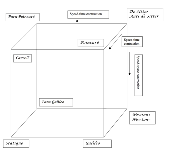
Figure 1: Eleven relativities connected through three types of contraction bacryjmll68

So far, we have examined the physical meaning of the quantities given in (III.23), (III.24), and (III.25). With their analytic descriptions (III.19), (III.20), and (III.21), they have to be understood as basic smooth observables on the six-dimensional Kählerian phase-space $\mathcal{D}^{(3)}$ for a free “massive” elementary system living in AdS₄ spacetime. With the parametrizations (III.23), (III.24), and (III.25), they are given a precise physical meaning in terms of the motion of an elementary system on AdS₄ spacetime. The function $k^{0}$ (III.19) should be understood as defining the Hamiltonian flow. The vector-valued function $\boldsymbol{\varsigma}$ (III.20) is associated with the classical orbital angular momentum and spin, while the complex-vector valued function $\boldsymbol{k}$ (III.21) defines the flows for AdS₄ hyperbolic rotations (real part), understood as “space translations”, and “Lorentz boost” (imaginary part). The two constraints defining the orbit class $\mathcal{O}(2\ell X_{0})$ in (III.15) are understood as the conservation of the energy and total angular momentum. They extend the familiar conservation laws for the free motion of a massive particle in flat Minkowskian spacetime to the motion in AdS₄ spacetime. As basic observables, they form an algebra closed under a Poisson bracket. The latter is determined by the form (II.81):

$$\{f,g\}=-\frac{\mathrm{i}}{2}h^{ij}\,\frac{\partial f}{\partial z^{i}}\frac{\partial g}{\partial\overline{z^{j}}}\equiv\boldsymbol{\omega}^{ij}\,\frac{\partial f}{\partial z^{i}}\frac{\partial g}{\partial\overline{z^{j}}}\,.$$ (III.44)

This algebra is in one-to-one correspondence with $\mathfrak{sp}(4,{\mathbb{R}})$ (for the latter, see (III)) in such a way that, in agreement with the Lie commutators (II.54), we have:

$$\left\{k^{0},\alpha^{i}\right\}=\beta^{i}\,,\quad\left\{k^{0},\beta^{i}\right\}=-\alpha^{i}\,,\quad\left\{\alpha^{j},\varsigma^{k}\right\}=-\alpha^{i}\,,$$

$$\left\{\alpha^{i},\beta^{i}\right\}=-k^{0}\,,\quad\left\{\varsigma^{k},\beta^{i}\right\}=\beta^{j}\,,\quad\left\{\varsigma^{k},\varsigma^{j}\right\}=-\varsigma^{i}\,.$$ (III.45)

We finally describe how the quantities $k^{0}$ (III.19), $\boldsymbol{\varsigma}$ (III.20), and $\boldsymbol{k}$ (III.21), i.e., the basic “classical observables”, transform under the (co-)adjoint representation (III.7) of Sp$(4,{\mathbb{R}})$. Hence, from

$$\mathfrak{sp}(4,{\mathbb{R}})\ni\mathsf{X}=\begin{pmatrix}\mathrm{i}k^{0}+\boldsymbol{\varsigma}\boldsymbol{k}\\ -\overline{\boldsymbol{k}}-\mathrm{i}k^{0}+\boldsymbol{\varsigma}\end{pmatrix}\;\mapsto\;\mathsf{X}^{\prime}=g\mathsf{X}g^{-1}=\begin{pmatrix}\mathrm{i}k^{\prime 0}+\boldsymbol{\varsigma}^{\prime}&\boldsymbol{k}^{\prime}\\ -\overline{\boldsymbol{k}^{\prime}}-\mathrm{i}k^{\prime 0}+\boldsymbol{\varsigma}^{\prime}\end{pmatrix}\,,$$ (III.46)

we get

$$k^{\prime 0} =k^{0}(\|a\|^{2}+\|b\|^{2})-\mathrm{i}\left(a\boldsymbol{\varsigma}a^{\ast}\right)_{\mathrm{s}}+\mathrm{i}\left(b\boldsymbol{\varsigma}b^{\ast}\right)_{\mathrm{s}}+\mathrm{i}\left(a\boldsymbol{k}b^{\ast}\right)_{\mathrm{s}}+\mathrm{i}\left(b\overline{\boldsymbol{k}}a^{\ast}\right)_{\mathrm{s}}\,,$$ (III.47)

$$\boldsymbol{\varsigma}^{\prime} =\mathrm{i}k^{0}(aa^{\ast}+bb^{\ast})_{\mathrm{v}}+(a\boldsymbol{\varsigma}a^{\ast})_{\mathrm{v}}-(b\boldsymbol{\varsigma}b^{\ast})_{\mathrm{v}}-(a\boldsymbol{k}b^{\ast})_{\mathrm{v}}-(b\overline{\boldsymbol{k}}a^{\ast})_{\mathrm{v}}\,,$$ (III.48)

$$\boldsymbol{k}^{\prime} =2\mathrm{i}k^{0}(a\widetilde{b})_{\mathrm{v}}+2(a\boldsymbol{\varsigma}\widetilde{b})_{\mathrm{v}}+a\boldsymbol{k}\widetilde{a}-b\overline{\boldsymbol{k}}\widetilde{b}\,,$$ (III.49)

where we have used the notations $(z)_{\mathrm{s}}$ and $(z)_{\mathrm{v}}$ respectively for the scalar and vector parts of the complex quaternion $z$, i.e., $z=\big{(}z_{0}\equiv(z)_{\mathrm{s}},\boldsymbol{z}\equiv(z)_{\mathrm{v}}\big{)}$.

Accordingly, the particular actions with respect to the subgroups involved in the time-space-Lorentz decomposition (II.47) of the group read:

• Temporal rotations: $h(\theta)\,:\,\mathsf{X}\;\mapsto\;\mathsf{X}^{\prime}\;\;$ with

  $$\begin{array}[]{rcl}k^{\prime 0}&=&k^{0}\\[1.45094pt] \boldsymbol{\varsigma}^{\prime}&=&\boldsymbol{\varsigma}\\[1.42271pt] \boldsymbol{k}^{\prime}&=&e^{\mathrm{i}\theta}\boldsymbol{k}\end{array}\,.$$ (III.50)

• Spatial rotations: $r(\xi):\mathsf{X}\;\mapsto\;\mathsf{X}^{\prime}\;\;$ with

  $$\begin{array}[]{rcl}k^{\prime 0}&=&k^{0}\\[1.42271pt] \boldsymbol{\varsigma}^{\prime}&=&\xi\boldsymbol{\varsigma}\widetilde{\xi}\\[1.42271pt] \boldsymbol{k}^{\prime}&=&\xi\boldsymbol{k}\widetilde{\xi}\end{array}\,.$$ (III.51)

• Spatial hyperbolic rotations: $s(\varrho,\hat{\boldsymbol{u}})\;:\;\mathsf{X}\;\mapsto\;\mathsf{X}^{\prime}$ with

  $$\begin{array}[]{rcl}k^{\prime 0}&=&k^{0}\cosh\varrho-\boldsymbol{\beta}\cdot\hat{\boldsymbol{u}}\,\sinh\varrho\\[1.42271pt] \boldsymbol{\varsigma}^{\prime}&=&\boldsymbol{\varsigma}\,\cosh^{2}\frac{\varrho}{2}+(-\hat{\boldsymbol{u}}\cdot\boldsymbol{\varsigma}\,\hat{\boldsymbol{u}}+\hat{\boldsymbol{u}}\times\boldsymbol{\varsigma}\times\hat{\boldsymbol{u}})\,\sinh^{2}\frac{\varrho}{2}+\boldsymbol{\alpha}\times\hat{\boldsymbol{u}}\,\sinh\varrho\\[1.42271pt] \boldsymbol{k}^{\prime}&=&-\mathrm{i}\hat{\boldsymbol{u}}\,k^{0}\sinh\varrho-\boldsymbol{\varsigma}\times\hat{\boldsymbol{u}}\,\sinh\varrho+\boldsymbol{k}\,\cosh^{2}\frac{\varrho}{2}+(-\hat{\boldsymbol{u}}\cdot\overline{\boldsymbol{k}}\,\hat{\boldsymbol{u}}+\hat{\boldsymbol{u}}\times\overline{\boldsymbol{k}}\times\hat{\boldsymbol{u}})\,\sinh^{2}\frac{\varrho}{2}\end{array}\,.$$ (III.52)

• Lorentz boosts: $\lambda(\nu,\hat{\boldsymbol{v}})\;:\;\mathsf{X}\;\mapsto\;\mathsf{X}^{\prime}\;\;$ with

  $$\begin{array}[]{rcl}k^{\prime 0}&=&k^{0}\cosh\nu-\boldsymbol{\alpha}\cdot\hat{\boldsymbol{v}}\,\sinh\nu\\[1.42271pt] \boldsymbol{\varsigma}^{\prime}&=&\boldsymbol{\varsigma}\,\cosh^{2}\frac{\nu}{2}+(-\hat{\boldsymbol{v}}\cdot\boldsymbol{\varsigma}\,\hat{\boldsymbol{v}}+\hat{\boldsymbol{v}}\times\boldsymbol{\varsigma}\times\hat{\boldsymbol{v}})\,\sinh^{2}\frac{\nu}{2}-\boldsymbol{\beta}\times\hat{\boldsymbol{v}}\,\sinh\nu\\[1.42271pt] \boldsymbol{k}^{\prime}&=&\hat{\boldsymbol{v}}\,k^{0}\sinh\nu-\mathrm{i}\boldsymbol{\varsigma}\times\hat{\boldsymbol{v}}\,\sinh\nu+\boldsymbol{k}\,\cosh^{2}\frac{\nu}{2}+(\hat{\boldsymbol{v}}\cdot\overline{\boldsymbol{k}}\,\hat{\boldsymbol{v}}-\hat{\boldsymbol{v}}\times\overline{\boldsymbol{k}}\times\hat{\boldsymbol{v}})\,\sinh^{2}\frac{\nu}{2}\end{array}\,.$$ (III.53)

The above actions should be compared with the representation of Sp$(4,{\mathbb{R}})$ as operators acting on the classical observables $f(\boldsymbol{z})$ as:

$$\mathrm{Sp}(4,{\mathbb{R}})\ni g\,:\,f(\boldsymbol{z})\;\mapsto\;f^{\prime}(\boldsymbol{z})\equiv f\left(g^{-1}\diamond\boldsymbol{z}\right)\,,$$ (III.54)

with the definition (II.77).

III.2 “Massive” “spin” (co-)adjoint orbits

Taking steps parallel to the above, in this subsection, we study a class of the Sp$(4,{\mathbb{R}})$ (co-)adjoint orbits, each being relevant to the transport of the element $\big{(}2\ell X_{0}+2\jmath Y_{3}\big{)}=\begin{pmatrix}\mathrm{i}\,\ell+\jmath\,\boldsymbol{e}_{3}&0\\ 0&-\mathrm{i}\,\ell+\jmath\,\boldsymbol{e}_{3}\end{pmatrix}$ of $\mathfrak{sp}(4,{\mathbb{R}})$ (see (II.48) and (II.50)), with $\ell,\jmath\in{\mathbb{R}}-\{0\}$, under the (co-)adjoint action (III.7). In this case, the stabilizer subgroup is a subgroup of $S_{2\ell X_{0}}=K$ (II.63):

$$S_{2\ell X_{0}+2\jmath Y_{3}}=\left\{h(\theta)\,r\big{(}\xi^{(\not{1}\not{2})}\big{)}\,,\,-\pi\leqslant\theta<\pi\,,\,\xi^{(\not{1}\not{2})}\,\in\mathrm{U}(1)\right\}\sim\mathrm{S}\big{(}\mathrm{U}(1)\times\mathrm{U}(1)\big{)}\,,$$ (III.55)

where $\xi^{(\not{1}\not{2})}:=\xi^{4}+\xi^{3}\boldsymbol{e}_{3}$ (i,e, $\xi^{1}=\xi^{2}=0$) and since $\xi^{(\not{1}\not{2})}\in\mathrm{U}(1)$ then $\xi^{4},\xi^{3}\in{\mathbb{R}}$ and $(\xi^{4})^{2}+(\xi^{3})^{2}=1$. Therefore, this class of the Sp$(4,{\mathbb{R}})$ (co-)adjoint orbits can be realized as a homogeneous space homeomorphic to the group coset $\mathcal{O}\big{(}2\ell X_{0}+2\jmath Y_{3}\big{)}\sim\mathrm{Sp}(4,{\mathbb{R}})/\mathrm{S}\big{(}\mathrm{U}(1)\times\mathrm{U}(1)\big{)}\sim\mathcal{D}^{(3)}\times\mathbb{S}^{2}$.

Technically, again with respect to the time-space-Lorentz factorization (II.47) of the group, this realization can be achieved by transporting the element ($2\ell X_{0}+2\jmath Y_{3}$) under the (co-)adjoint action (III.7), when $g$ involved in the action belongs to the subgroup

$$L^{(\not{3})}_{sbr}=\{s(\varrho,\hat{\boldsymbol{u}})\,\lambda(\nu,\hat{\boldsymbol{v}})\,r\big{(}\xi^{(\not{3})}\big{)}\,;\;\varrho,\nu\in{\mathbb{R}}^{+},\;\hat{\boldsymbol{u}},\hat{\boldsymbol{v}}\in\mathbb{S}^{2},\;\xi^{(\not{3})}\in\mathrm{SU}(2)/\mathrm{U}(1)\sim\mathbb{S}^{2}\}$$ (III.56)

such that $s(\varrho,\hat{\boldsymbol{u}})$ and $\lambda(\nu,\hat{\boldsymbol{v}})$ are given in Eq. (III.10), and $r\big{(}\xi^{(\not{3})\big{)}}$ is given in Eq. (II.64) with $\xi^{(\not{3})}:=\xi^{4}+\xi^{1}\boldsymbol{e}_{1}+\xi^{2}\boldsymbol{e}_{2}$ such that $\xi^{4},\xi^{1},\xi^{2}\in{\mathbb{R}}$ and $(\xi^{4})^{2}+(\xi^{1})^{2}+(\xi^{2})^{2}=1$.

Accordingly the (co-)adjoint action gives:

$$\mbox{Ad}_{g}\big{(}2\ell X_{0}+2\jmath Y_{3}\big{)} = s(\varrho,\hat{\boldsymbol{u}})\;\lambda(\nu,\hat{\boldsymbol{v}})\;r\big{(}\xi^{(\not{3})}\big{)}\;\Big{(}2\ell X_{0}+2\jmath Y_{3}\Big{)}\;r^{-1}\big{(}\xi^{(\not{3})}\big{)}\;\lambda^{-1}(\nu,\hat{\boldsymbol{v}})\;s^{-1}(\varrho,\hat{\boldsymbol{u}})$$ (III.57)

$$= \begin{pmatrix}\mathrm{i}k^{0}+\boldsymbol{\varsigma}&\boldsymbol{k}\\ -\overline{\boldsymbol{k}}&-\mathrm{i}k^{0}+\boldsymbol{\varsigma}\end{pmatrix}=\mathsf{X}(k^{0},\boldsymbol{\varsigma},\boldsymbol{k})\,,$$

where:

$$\begin{array}[]{lll}k^{0}&=&\ell\,\cosh\varrho\cosh\nu-\jmath\,\sinh\varrho\sinh\nu\,\big{(}\hat{\boldsymbol{u}},\hat{\boldsymbol{v}},\hat{\boldsymbol{\xi}}\big{)}\,,\\[8.5359pt] \boldsymbol{\varsigma}&=&\ell\,\sinh\varrho\sinh\nu\,\big{(}\hat{\boldsymbol{v}}\times\hat{\boldsymbol{u}}\big{)}\\[4.26773pt] &&\;\;+\;\jmath\,\Bigg{(}\cosh\nu\bigg{[}\cosh\rho\,\hat{\boldsymbol{\xi}}_{\perp\hat{\boldsymbol{v}}}-(\cosh\rho-1)\Big{(}(\hat{\boldsymbol{u}}\cdot\hat{\boldsymbol{\xi}})-(\hat{\boldsymbol{v}}\cdot\hat{\boldsymbol{\xi}})(\hat{\boldsymbol{u}}\cdot\hat{\boldsymbol{v}})\Big{)}\hat{\boldsymbol{u}}\bigg{]}\\[4.26773pt] &&\qquad\qquad+\,(\hat{\boldsymbol{v}}\cdot\hat{\boldsymbol{\xi}})\Big{(}\cosh\rho\,\hat{\boldsymbol{v}}_{\perp\hat{\boldsymbol{u}}}+\;(\hat{\boldsymbol{u}}\cdot\hat{\boldsymbol{v}})\hat{\boldsymbol{u}}\Big{)}\Bigg{)}\,,\\[8.5359pt] \boldsymbol{k}=\boldsymbol{\alpha}+\mathrm{i}\boldsymbol{\beta}&=&\ell\Big{(}\hat{\boldsymbol{v}}\cosh^{2}\frac{\varrho}{2}\sinh\nu+\hat{\boldsymbol{u}}\hat{\boldsymbol{v}}\hat{\boldsymbol{u}}\sinh^{2}\frac{\varrho}{2}\sinh\nu-\mathrm{i}\hat{\boldsymbol{u}}\sinh{\varrho}\cosh\nu\Big{)}\\[4.26773pt] &&\;\;+\;\jmath\,\Bigg{(}\sinh\varrho\bigg{[}\cosh\nu\,(\hat{\boldsymbol{u}}\times\hat{\boldsymbol{\xi}}_{\perp\hat{\boldsymbol{v}}})+(\hat{\boldsymbol{v}}\cdot\hat{\boldsymbol{\xi}})(\hat{\boldsymbol{u}}\times\hat{\boldsymbol{v}})\bigg{]}\\[4.26773pt] &&\;\;\;\;\;\;+\;\mathrm{i}\,\sinh\nu\left((\hat{\boldsymbol{v}}\times\hat{\boldsymbol{\xi}})+(\cosh\varrho-1)\big{(}\hat{\boldsymbol{u}},\hat{\boldsymbol{v}},\hat{\boldsymbol{\xi}}\big{)}\,\hat{\boldsymbol{u}}\right)\Bigg{)}\,,\end{array}$$ (III.58)

where we have used the notations $\hat{\boldsymbol{\xi}}\equiv\xi^{(\not{3})}\,\boldsymbol{e}_{3}\,\widetilde{\xi^{(\not{3})}}\in\mathbb{S}^{2}$, $\big{(}\hat{\boldsymbol{u}},\hat{\boldsymbol{v}},\hat{\boldsymbol{\xi}}\big{)}\equiv\hat{\boldsymbol{u}}\cdot\big{(}\hat{\boldsymbol{v}}\times\hat{\boldsymbol{\xi}}\big{)}$, $\hat{\boldsymbol{u}}_{\parallel\hat{\boldsymbol{v}}}\equiv\hat{\boldsymbol{v}}\cdot\hat{\boldsymbol{u}}\,\hat{\boldsymbol{v}}$, $\hat{\boldsymbol{u}}_{\perp\hat{\boldsymbol{v}}}\equiv\hat{\boldsymbol{u}}-\hat{\boldsymbol{u}}_{\parallel\hat{\boldsymbol{v}}}$ and the formula $\hat{\boldsymbol{v}}\hat{\boldsymbol{u}}\hat{\boldsymbol{v}}=\hat{\boldsymbol{u}}-2\hat{\boldsymbol{u}}_{\parallel\hat{\boldsymbol{v}}}$.

With respect to the relations that hold between the matrix elements of $\mathsf{X}(k^{0},\boldsymbol{\varsigma},\boldsymbol{k})$, there are two constraints that determine the (co-)adjoint orbit class $\mathcal{O}\big{(}2\ell X_{0}+2\jmath Y_{3}\big{)}$ of Sp$(4,{\mathbb{R}})$ in the (dual of) its Lie algebra $\mathfrak{sp}(4,{\mathbb{R}})$:

$$\ell^{2}+\jmath^{2} = (k^{0})^{2}-\|\boldsymbol{k}\|^{2}+\|\boldsymbol{\varsigma}\|^{2}\,,$$ (III.59)

$$\big{(}\ell^{2}-\jmath^{2}\big{)}^{2} = \det(\mathrm{i}k^{0}+\boldsymbol{\varsigma})\det\Big((-\mathrm{i}k^{0}+\boldsymbol{\varsigma})+\overline{\boldsymbol{k}}(\mathrm{i}k^{0}+\boldsymbol{\varsigma})^{-1}\boldsymbol{k}\Big{missing})=\Big{(}(k^{0})^{2}-\|\boldsymbol{k}\|^{2}-\|\boldsymbol{\varsigma}\|^{2}\Big{)}^{2}\,,$$ (III.60)

where, to derive the latter equation, we have employed the identity (II.75). Then, $\mathcal{O}\big{(}2\ell X_{0}+2\jmath Y_{3}\big{)}$ can be viewed as:

$$\mathcal{O}\big{(}2\ell X_{0}+2\jmath Y_{3}\big{)}=\left\{(k^{0},\boldsymbol{\varsigma},\boldsymbol{k})\,;\,\ell^{2}+\jmath^{2}=(k^{0})^{2}-\|\boldsymbol{k}\|^{2}+\|\boldsymbol{\varsigma}\|^{2}\,,\;\big{(}\ell^{2}-\jmath^{2}\big{)}^{2}=\Big{(}(k^{0})^{2}-\|\boldsymbol{k}\|^{2}-\|\boldsymbol{\varsigma}\|^{2}\Big{)}^{2}\right\}\,.$$ (III.61)

The application of the constraints (III.59) and (III.60) leads to the existence of three distinct and independent scenarios:

1. Case $l^{2}=\jmath^{2}$. Then, in a physically relevant case, we have:

   $$l^{2}=\jmath^{2}=(k^{0})^{2}-\|\boldsymbol{k}\|^{2}=\|\boldsymbol{\varsigma}\|^{2}\,.$$ (III.62)

2. Cases $l^{2}>\jmath^{2}$ and $(k^{0})^{2}-\|\boldsymbol{k}\|^{2}-\|\boldsymbol{\varsigma}\|^{2}>0$ or $l^{2}<j^{2}$ and $(k^{0})^{2}-\|\boldsymbol{k}\|^{2}-\|\boldsymbol{\varsigma}\|^{2}<0$. Then:

   $$\ell^{2}=(k^{0})^{2}-\|\boldsymbol{k}\|^{2}\,,\qquad\jmath^{2}=\|\boldsymbol{\varsigma}\|^{2}\,.$$ (III.63)

3. Cases $l^{2}>\jmath^{2}$ and $(k^{0})^{2}-\|\boldsymbol{k}\|^{2}-\|\boldsymbol{\varsigma}\|^{2}<0$ or $l^{2}<j^{2}$ and $(k^{0})^{2}-\|\boldsymbol{k}\|^{2}-\|\boldsymbol{\varsigma}\|^{2}>0$. Then:

   $$\ell^{2}=\|\boldsymbol{\varsigma}\|^{2}\,,\qquad\jmath^{2}=(k^{0})^{2}-\|\boldsymbol{k}\|^{2}\,.$$ (III.64)

Each case corresponds to a distinct sub-manifold of the (co-)adjoint orbit $\mathcal{O}\big{(}2\ell X_{0}+2\jmath Y_{3}\big{)}$. Now, let us proceed with the first two scenarios that are both physically relevant and also consistent with the scalar case (III.13). As before, we associate appropriate physical dimensions to the involved variables as follows (recall that $\boldsymbol{k}=\boldsymbol{\alpha}+\mathrm{i}\boldsymbol{\beta}$):

$$k^{0} = \ell\,\frac{E}{mc^{2}}\,,$$ (III.65)

$$\boldsymbol{\alpha} = \ell\,{\varkappa}\,\boldsymbol{q}\,,\hskip 56.9055pt\ell\in{\mathbb{R}}^{+}\,,$$ (III.66)

$$\boldsymbol{\beta} = \ell\,\frac{\boldsymbol{p}}{mc}\,,$$ (III.67)

It is important to note that the parameter $\jmath$ is intentionally left separate as it is equal to $\pm\|\boldsymbol{\varsigma}\|$, and so is associated with the concept of classical spin. Then, in case (i) (resp. (ii)), the (co-)adjoint orbit class (III.62) (resp. (III.63)) can be interpreted as the phase space for “massless” (resp. “massive”) spin elementary systems living in AdS₄ spacetime. These co-adjoint orbits are Cartesian products of a two-dimensional sphere, with radius $|\jmath|$, with a six-dimensional two-sheeted hyperboloid in ${\mathbb{R}}^{7}$, equipped with the metric diag$(+,-,-,-,-,-,-)$ and with radius $\ell$. In this context, the constraint $\ell^{2}=(k^{0})^{2}-\|\boldsymbol{k}\|^{2}$ turns into:

$$E^{2}=m^{2}c^{4}+c^{2}\|\boldsymbol{p}\|^{2}+m^{2}c^{4}{\varkappa}^{2}\|\boldsymbol{q}\|^{2}\,.$$ (III.68)

Under the null-curvature (Poincaré) limit, as ${\varkappa}\rightarrow 0$, this constraint clearly meets the mass shell hyperboloid (III.30), and under non-relativistic (Newtonian) limit, as $c\to\infty$ and ${\varkappa}\to 0$ ($c{\varkappa}=\mathrm{constant}\equiv\omega$), the identity (III.43).

IV Sp$(4,{\mathbb{R}})$ representation(s) in the discrete series

In this section, we study the construction of the AdS₄ UIRs relevant to the quantum reading of the described classical systems above. The so-called “massive” elementary systems living in AdS₄ spacetime on the quantum level are associated with the discrete series UIRs $U^{(\varsigma,s)}$ of Sp$(4,{\mathbb{R}})$ or of its universal covering $\overline{\mathrm{Sp}(4,{\mathbb{R}})}$ evans67 ; fronsdal74 ; baelgagi92 ; Gazeau2022 ; Dobrev1 ; Dobrev2 ; the parameters $\varsigma\in{\mathbb{R}}_{+}$ and $s\in{\mathbb{N}}/2$ (spin) are dimensionless, and satisfy $\varsigma>s+1$ (the lowest limit $\varsigma=s+1$ is the “massless” case). For $\varsigma>s+2$, the representation Hilbert spaces are denoted by Fock-Bargmann spaces $\mathcal{F}^{(\varsigma,s)}$ and their elements are holomorphic $(2s+1)$-vector functions:

$$\mathcal{D}^{(3)}\ni\boldsymbol{z}\;\mapsto\;f(\boldsymbol{z})\in{\mathbb{C}}^{2s+1}\,,$$ (IV.1)

that are square integrable with respect to the bilinear form:

$$(f_{1},f_{2})_{(\varsigma,s)}=\mathcal{N}(\varsigma,s)\int_{\mathcal{D}^{(3)}}f_{1}(\boldsymbol{z})^{{\dagger}}\,D^{s}\left(\frac{1}{1+\boldsymbol{z}\overline{\boldsymbol{z}}}\right)\,f_{2}(\boldsymbol{z})\,\big{[}\det(1+\boldsymbol{z}\overline{\boldsymbol{z}})\big{]}^{\varsigma+s-3}\,d{\boldsymbol{z}}\,,\quad d{\boldsymbol{z}}\equiv\mathrm{d}^{3}\boldsymbol{x}\,\mathrm{d}^{3}\boldsymbol{y}\,.$$ (IV.2)

Note that: (i) The operator $D^{s}$ is the holomorphic extension to $\mathrm{M}(2,{\mathbb{C}})$ of the irreducible $(2s+1)\times(2s+1)$-matrix representation of the SU$(2)$ group. (ii) The constant $\mathcal{N}(\varsigma,s)$ is chosen in such a way that the particular $(2s+1)$-vector-valued constant function $e_{ss}$ when the general $e_{s\rho}$, with $-s\leqslant\rho\leqslant s$, is defined by:

$$\begin{array}[]{lll}&\mbox{for integer $s$}:&e_{s\rho}\equiv\left(\delta_{s,\rho},\,\delta_{s-1,\rho},\,\dots\,,\,\delta_{1,\rho},\,\delta_{0,\rho},\,\delta_{-1,\rho},\,\dots\,,\,\delta_{-s+1,\rho},\,\delta_{-s,\rho}\right)^{\mathrm{t}}\,,\\[8.5359pt] &\mbox{for half-integer $s$}:&e_{s\rho}\equiv\left(\delta_{s,\rho},\,\delta_{s-1,\rho},\,\dots\,,\,\delta_{\frac{1}{2},\rho},\,\delta_{-\frac{1}{2},\rho},\,\dots\,,\,\delta_{-s+1,\rho},\,\delta_{-s,\rho}\right)^{\mathrm{t}},\end{array}$$ (IV.3)

has norm one (${\mathrm{t}}$ stands for the transpose). This constant is given by (see, for instance, Ref. onofri76 ):

$$\mathcal{N}(\varsigma,s)=\frac{8}{\pi^{3}}\,\left(\varsigma+s-\frac{3}{2}\right)\,(\varsigma-s-1)\,(\varsigma-s-2)\,.$$ (IV.4)

(iii) Modification of the inner product is required for the range $s+1\leqslant\varsigma\leqslant s+2$, where the Shilov boundary $[0,\pi]\times\mathbb{S}^{2}$ (i.e., the Lie sphere) of $\mathcal{D}^{(3)}$ plays a crucial rôle onofri76 .

The operators of the UIRs $U^{(\varsigma,s)}$ of Sp$(4,{\mathbb{R}})$ are defined by the following action on the functions $f$ of $\mathcal{F}^{(\varsigma,s)}$:

$$\begin{split}f^{\prime}(\boldsymbol{z})=\left(U^{(\varsigma,s)}(g)\,f\right)(\boldsymbol{z})=\big{[}\det(-\overline{b}\boldsymbol{z}+\overline{a})\big{]}^{-\varsigma-s}\,D^{s}(\boldsymbol{z}b^{\ast}+a^{\ast})\,f\left(g^{-1}\diamond\boldsymbol{z}\right)\,,\end{split}$$ (IV.5)

with $g^{-1}=\begin{pmatrix}a&b\\ -\overline{b}&\overline{a}\end{pmatrix}$ and $g^{-1}\diamond\boldsymbol{z}=(a\boldsymbol{z}+b)(-\overline{b}\boldsymbol{z}+\overline{a})^{-1}$, where here for convenience we consider $g^{-1}$ in the opposite way to the usual notations following Eqs. (II.21) and (II.22).

When multiplied by $\mathrm{i}$, the $10$ infinitesimal generators of the action (IV.5) span a representation of the Lie algebra $\mathfrak{sp}(4,{\mathbb{R}})$ by self-adjoint operators $L_{\alpha\beta}$ in $\mathcal{F}^{(\varsigma,s)}$, with the decomposition in orbital and spin parts:

$$\mathfrak{sp}(4,{\mathbb{R}})\ni N_{\alpha\beta}\;\mapsto\;L_{\alpha\beta}=M_{\alpha\beta}+S_{\alpha\beta}\,.$$ (IV.6)

According to the Stone theorem Stone , their respective expressions read:

$$L_{50} =\left(\boldsymbol{z}\cdot\boldsymbol{\nabla}_{\boldsymbol{z}}+\varsigma\right)\mathbbm{1}_{2s+1}\,,\qquad\boldsymbol{\nabla}_{\boldsymbol{z}}=\left(\frac{\partial}{\partial z^{1}},\frac{\partial}{\partial z^{2}},\frac{\partial}{\partial z^{3}}\right)\,,$$ (IV.7)

$$L_{12} =\mathrm{i}\left(z^{1}\frac{\partial}{\partial z^{2}}-z^{2}\frac{\partial}{\partial z^{1}}\right)\mathbbm{1}_{2s+1}-S_{3}\,,$$ (IV.8)

$$L_{23} =\mathrm{i}\left(z^{2}\frac{\partial}{\partial z^{3}}-z^{3}\frac{\partial}{\partial z^{2}}\right)\mathbbm{1}_{2s+1}-S_{1}\,,$$ (IV.9)

$$L_{31} =\mathrm{i}\left(z^{3}\frac{\partial}{\partial z^{1}}-z^{1}\frac{\partial}{\partial z^{3}}\right)\mathbbm{1}_{2s+1}-S_{2}\,,$$ (IV.10)

$$L_{51} =\mathrm{i}\left(\frac{1+\boldsymbol{z}\cdot\boldsymbol{z}}{2}\frac{\partial}{\partial z^{1}}-z^{1}\left(\varsigma+s+\boldsymbol{z}\cdot\boldsymbol{\nabla}_{\boldsymbol{z}}\right)\right)\mathbbm{1}_{2s+1}+z^{2}S_{3}-z^{3}S_{2}\,,$$ (IV.11)

$$L_{52} =\mathrm{i}\left(\frac{1+\boldsymbol{z}\cdot\boldsymbol{z}}{2}\frac{\partial}{\partial z^{2}}-z^{2}\left(\varsigma+s+\boldsymbol{z}\cdot\boldsymbol{\nabla}_{\boldsymbol{z}}\right)\right)\mathbbm{1}_{2s+1}-z^{1}S_{3}+z^{3}S_{1}\,,$$ (IV.12)

$$L_{53} =\mathrm{i}\left(\frac{1+\boldsymbol{z}\cdot\boldsymbol{z}}{2}\frac{\partial}{\partial z^{3}}-z^{3}\left(\varsigma+s+\boldsymbol{z}\cdot\boldsymbol{\nabla}_{\boldsymbol{z}}\right)\right)\mathbbm{1}_{2s+1}+z^{1}S_{2}-z^{2}S_{1}\,,$$ (IV.13)

$$L_{01} =-\left(\frac{1-\boldsymbol{z}\cdot\boldsymbol{z}}{2}\frac{\partial}{\partial z^{1}}+z^{1}\left(\varsigma+s+\boldsymbol{z}\cdot\boldsymbol{\nabla}_{\boldsymbol{z}}\right)\right)\mathbbm{1}_{2s+1}-\mathrm{i}z^{2}S_{3}+\mathrm{i}z^{3}S_{2}\,,$$ (IV.14)

$$L_{02} =-\left(\frac{1-\boldsymbol{z}\cdot\boldsymbol{z}}{2}\frac{\partial}{\partial z^{2}}+z^{2}\left(\varsigma+s+\boldsymbol{z}\cdot\boldsymbol{\nabla}_{\boldsymbol{z}}\right)\right)\mathbbm{1}_{2s+1}+\mathrm{i}z^{1}S_{3}-\mathrm{i}z^{3}S_{1}\,,$$ (IV.15)

$$L_{03} =-\left(\frac{1-\boldsymbol{z}\cdot\boldsymbol{z}}{2}\frac{\partial}{\partial z^{3}}+z^{3}\left(\varsigma+s+\boldsymbol{z}\cdot\boldsymbol{\nabla}_{\boldsymbol{z}}\right)\right)\mathbbm{1}_{2s+1}-\mathrm{i}z^{1}S_{2}+\mathrm{i}z^{2}S_{1}\,.$$ (IV.16)

The $(2s+1)\times(2s+1)$-matrices $S_{1}$, $S_{2}$, and $S_{3}$ in the above are given respectively by:

$$(S_{1})_{mm^{\prime}} =\frac{1}{2}\sqrt{(s+m)(s-m+1)}\,\delta_{m,m^{\prime}+1}+\frac{1}{2}\sqrt{(s-m)(s+m+1)}\,\delta_{m,m^{\prime}-1}\,,$$ (IV.17)

$$(S_{2})_{mm^{\prime}} =\frac{1}{2\mathrm{i}}\sqrt{(s-m)(s+m+1)}\,\delta_{m,m^{\prime}-1}-\frac{1}{2\mathrm{i}}\sqrt{(s+m)(s-m+1)}\,\delta_{m,m^{\prime}+1}\,,$$ (IV.18)

$$(S_{3})_{mm^{\prime}} =m\,\delta_{mm^{\prime}}\,,$$ (IV.19)

for $m$ and $m^{\prime}$ such that $-s\leqslant m,m^{\prime}\leqslant s$. They realize the spin $s$ representation of the Lie algebra $\mathfrak{su}(2)$:

$$\left[S_{i},S_{j}\right]=\mathrm{i}\epsilon_{ij}^{\,\,k}S_{k}\,,\quad i,j,k\in\{1,2,3\}\,.$$ (IV.20)

Considering the above, one checks that the generators $L_{\alpha\beta}$ satisfy the quantum version of the commutation rules (II.54) (up to the factor $\mathrm{i}$):

$$\left[L_{\alpha\beta},L_{\gamma\rho}\right]=\mathrm{i}\left(\eta_{\alpha\gamma}{L_{\beta\rho}}+\eta_{\beta\rho}{L_{\alpha\gamma}}-\eta_{\alpha\rho}{L_{\beta\gamma}}-\eta_{\beta\gamma}{L_{\alpha\rho}}\right)\,.$$ (IV.21)

Like for the Poincaré group, kinematical group the Minkowski spacetime, there exist two invariants that characterize each UIR of the AdS₄ group. They are the second-order and quartic-order Casimir operators respectively defined by:

$$Q^{(1)}=-\frac{1}{2}L_{\alpha\beta}L^{\alpha\beta}\,,\qquad Q^{(2)}=-W_{\alpha}W^{\alpha},$$ (IV.22)

where $W_{\alpha}\equiv-\frac{1}{8}\epsilon_{\alpha\beta\gamma\delta\eta}L^{\beta\gamma}L^{\delta\eta}$. Taking into account the above infinitesimal generators (IV.7)-(IV.16), the eigenvalues of the two Casimir operators, completely determining the UIRs $U^{(\varsigma,s)}$, read as:

$$\langle Q^{(1)}\rangle=\varsigma(\varsigma-3)+s(s+1)\,,\qquad\langle Q^{(2)}\rangle=-(\varsigma-1)(\varsigma-2)s(s+1)\,.$$ (IV.23)

The very point to be noticed here is that $L_{50}=M_{50}$ is the ladder operator for the UIR parameter $\varsigma$. Its eigenvalues are $\varsigma,\varsigma+1,\varsigma+2,\dotsc,\varsigma+n,\dotsc$, which means that $U^{(\varsigma,s)}$ is a lowest-weight representation in the discrete series. Since $\varsigma$ is the lowest value of the discrete spectrum of the generator of “time” rotations in AdS₄ spacetime, it is naturally given a non-ambiguous meaning of a rest energy when it is expressed in the energy AdS₄ units $\hbar{\varkappa}c$ ($\hbar$ and $c$ respectively being the Planck constant and the speed of light):

$$E^{\mathrm{rest}}_{\text{\tiny{AdS${}_{4}$}}}\equiv\hbar c{\varkappa}\,\varsigma\,.$$ (IV.24)

Therefore, the physical concept of “energy at rest” survives with the deformation Poincaré $\longrightarrow$ AdS₄. In a shortcut (see the details in subsection IV.2), we would like to point out that, at the difference with the flat spacetime limit, $E^{\mathrm{rest}}_{\text{\tiny{AdS${}_{4}$}}}$ is not restricted to the pure mass energy (proper mass of the system), actually it includes as well a kind of pure quantum vibration energy due to the curvature GazeauTannoudji2021 ; Gazeau2020 , as we have already seen in the classical case.

IV.1 Poincaré contraction limit

In this subsection, we describe the way in which the AdS₄ discrete series UIRs $U^{(\varsigma,s)}(g)$ become the massive Wigner UIRs $\mathcal{P}^{(m,s)}$ with mass $m$ and spin $s$ of the Poincaré group in the null-curvature limit, $\varkappa\to 0$. To do this, we take parallel steps to those given in Ref. GazeauHussinJPA (see also Refs. del Olmo 1997 ; De Bievre 1994 ; De Bievre 1993 ; De Bievre 1992 ; Karim 1996 ) for such a limit of the AdS₂ discrete series UIRs, for which we need to consider the time-space-Lorentz decomposition (II.47) of the group, namely:

$$\mathrm{Sp}(4,{\mathbb{R}})\ni g=j(\theta,\varrho,\hat{\boldsymbol{u}})\,l(\xi,\nu,\hat{\boldsymbol{v}})=h(\theta)\,s(\varrho,\hat{\boldsymbol{u}})\,r(\xi)\,\lambda(\nu,\hat{\boldsymbol{v}})\,,$$ (IV.25)

(the explicit expression of the factors $h(\theta),\,r(\xi)),\,s(\varrho,\hat{\boldsymbol{u}})$ and $\lambda(\nu,\hat{\boldsymbol{v}})$ are given in (II.64) and (III.10)) and in more detail by introducing physical dimensions in the group parameters. Hence, we put:

$$\theta={\varkappa}\,c\,t\,,\qquad\varrho={\varkappa}\,x\,,\qquad\hat{\boldsymbol{v}}\,\tanh\frac{\nu}{2}=\frac{\mathfrak{\textbf{v}}}{c}\,,$$ (IV.26)

where $c$ is the speed of light, $x\in{\mathbb{R}}^{+}$, and $\mathfrak{\textbf{v}}\equiv\big{(}0,\mathfrak{\textbf{v}}\big{)}=\big{(}0,(\text{v}^{i})\big{)}\in\mathbb{H}$. Moreover, we consider the relation between the AdS₄ representation parameter $\varsigma$ and the Minkowski mass $m$ as Gazeau2020 ; GazeauTannoudji2021 ; Gazeau2022 :

$$\varsigma\equiv\varsigma({\varkappa})=\frac{mc}{\hbar{\varkappa}}+\frac{3}{2}+\left(s-\frac{1}{2}\right)^{2}\left(\frac{\hbar{\varkappa}}{2mc}+{\cal{O}}\left(\frac{{\varkappa}^{2}}{c^{2}}\right)\right)\,.$$ (IV.27)

From the latter identity, when the curvature ${\varkappa}$ goes to zero and subsequently $\varsigma$ goes to infinity, it is apparent that the bilinear form (IV.2) or equivalently the space $\mathcal{F}^{(\varsigma,s)}$ is not well adapted to such a limiting process. Thus, we introduce a ‘weighted’ Fock-Bargmann space:

$$\mathcal{F}^{(\varsigma,s)}_{W}=\left\{F(\boldsymbol{z},\overline{\boldsymbol{z}})=\big{[}\det(1+\boldsymbol{z}\overline{\boldsymbol{z}})\big{]}^{\frac{\varsigma+s}{2}}f(\boldsymbol{z})\,,\,f(\boldsymbol{z})\in\mathcal{F}^{(\varsigma,s)}\right\},$$ (IV.28)

where we have taken into account that $\det(1+\boldsymbol{z}\overline{\boldsymbol{z}})=\det(1+\overline{\boldsymbol{z}}\boldsymbol{z})$. This new function space is the Hilbert space of non-analytic functions inside $\mathcal{D}^{(3)}$, having the specific form (IV.28), and square-integrable with respect to:

$$(F_{1},F_{2})_{(\varsigma,s)}=\mathcal{N}(\varsigma,s)\,\int_{\mathcal{D}^{(3)}}F_{1}(\boldsymbol{z},\overline{\boldsymbol{z}})^{{\dagger}}\,D^{s}\left(\frac{1}{1+\boldsymbol{z}\overline{\boldsymbol{z}}}\right)\,F_{2}(\boldsymbol{z},\overline{\boldsymbol{z}})\,\big{[}\det(1+\boldsymbol{z}\overline{\boldsymbol{z}})\big{]}^{-3}\,d{\boldsymbol{z}}\,,$$ (IV.29)

(remember that $d{\boldsymbol{z}}\equiv\mathrm{d}^{3}\boldsymbol{x}\,\mathrm{d}^{3}\boldsymbol{y}$). The representation $U^{(\varsigma,s)}_{W}(g)$ on $\mathcal{F}^{(\varsigma,s)}_{W}$ is deduced from $U^{(\varsigma,s)}(g)$ given by (IV.5):

$$\begin{split}F^{\prime}(\boldsymbol{z},\overline{\boldsymbol{z}})=\left(U^{(\varsigma,s)}_{W}(g)\,F\right)(\boldsymbol{z},\overline{\boldsymbol{z}})=\left[\frac{\det(-b\overline{\boldsymbol{z}}+a)}{\det(-\overline{b}\boldsymbol{z}+\overline{a})}\right]^{\frac{\varsigma+s}{2}}\,D^{s}(\boldsymbol{z}b^{\ast}+a^{\ast})\,F\left(g^{-1}\diamond\boldsymbol{z},\overline{g^{-1}\diamond{\boldsymbol{z}}}\right)\,.\end{split}$$ (IV.30)

Note that, above, we have used the identity (II.89) and the fact that the above procedure must not change the homogeneity property of the former construction.

Now, in order to eliminate the singularity from $F(\boldsymbol{z},\overline{\boldsymbol{z}})$ (IV.28), we must impose some constraints on the form of the original analytic function $f(\boldsymbol{z})$. To do this, we factorize $f(\boldsymbol{z})$ as:

$$f(\boldsymbol{z})\equiv f(\boldsymbol{z},{\varkappa})=N({\varkappa})\,\big{[}\det(1+\boldsymbol{z}\widetilde{\boldsymbol{z}})\big{]}^{-\frac{\varsigma({\varkappa})+s}{2}}\,\check{f}(\boldsymbol{z},{\varkappa})\,,$$ (IV.31)

where the function $\check{f}$ is analytic in both $\boldsymbol{z}\in{\mathcal{D}}^{(3)}$ and ${\varkappa}\in{\mathbb{R}}^{+}$, $N({\varkappa})$ is a normalization factor possibly non-analytic in ${\varkappa}$. Note that, in the sequel, normalization will not be imposed in order to eliminate the term $N({\varkappa})$. The square-integrability condition then takes the form:

$$(\check{f}_{1},\check{f}_{2})^{\mbox{\small{reg}}}_{(\varsigma,s)}=\mathcal{N}(\varsigma,s)\int_{\mathcal{D}^{(3)}}\check{f}_{1}(\boldsymbol{z},{\varkappa})^{{\dagger}}\,D^{s}\left(\frac{1}{1+\boldsymbol{z}\overline{\boldsymbol{z}}}\right)\,\check{f}_{2}(\boldsymbol{z},{\varkappa})\,\left[\frac{\det(1+\boldsymbol{z}\overline{\boldsymbol{z}})}{|\det(1+\boldsymbol{z}\widetilde{\boldsymbol{z}})|}\right]^{\varsigma+s}\,\big{[}\det(1+\boldsymbol{z}\overline{\boldsymbol{z}})\big{]}^{-3}\,d{\boldsymbol{z}}\,.$$ (IV.32)

We accordingly restrict our considerations by working on the subspace of $\mathcal{F}^{(\varsigma,s)}_{W}$ which consists of functions of the form:

$$F(\boldsymbol{z},\overline{\boldsymbol{z}})=\left[\frac{\det(1+\boldsymbol{z}\overline{\boldsymbol{z}})}{\det(1+\boldsymbol{z}\widetilde{\boldsymbol{z}})}\right]^{\frac{\varsigma({\varkappa})+s}{2}}\check{f}(\boldsymbol{z})\,,\qquad\check{f}(\boldsymbol{z})\equiv\check{f}(\boldsymbol{z},\varkappa)\,.$$ (IV.33)

As the final stage before getting involved with the contraction limit, we set $\boldsymbol{z}\mapsto\boldsymbol{z}_{\mathrm{i}}\equiv-\mathrm{i}\boldsymbol{z}$. Then, the weight regular factor is such that:

$$\lim_{{\varkappa}\rightarrow 0}\left[\frac{\det(1+\boldsymbol{z}_{\mathrm{i}}\overline{\boldsymbol{z}_{\mathrm{i}}})}{\det(1+\boldsymbol{z}_{\mathrm{i}}\widetilde{\boldsymbol{z}_{\mathrm{i}}})}\right]^{\frac{\varsigma({\varkappa})+s}{2}}=1\,.$$ (IV.34)

The above formula can be easily checked through the parametrization of ${\mathcal{D}}^{(3)}$ in terms of $\boldsymbol{z}\equiv\boldsymbol{z}(p,q)\equiv\mbox{\eqref{invmom}}$, when we have in mind the dimensionless quantities introduced in Eqs. (III.23), (III.24) and (III.25); $\lim_{{\varkappa}\rightarrow 0}\boldsymbol{z}(p,q)\equiv\textbf{x}_{\circ}(p)$ is a purely real vector quaternion (see Eq. (III.34)), and hence, $\lim_{{\varkappa}\rightarrow 0}\boldsymbol{z}_{\mathrm{i}}(p,q)=-\mathrm{i}\textbf{x}_{\circ}(p)\equiv\textbf{x}_{\circ\mathrm{i}}(p)$ is a purely imaginary vector quaternion.

Having all the above in mind, we now consider the null-curvature limit of (IV.30) (when $\boldsymbol{z}\mapsto\boldsymbol{z}_{\mathrm{i}}$ and taking into account Eqs. (IV.33) and (IV.34)) in two steps:

• When $g$ is restricted to the “time-space translations” subgroup:

  • 1) The “time-translations” subgroup (see the first expression of (II.64) taking $\theta={\varkappa}ct$):

    $$h^{-1}({\varkappa}ct)=\begin{pmatrix}e^{-\mathrm{i}{\varkappa}ct/2}&0\\ 0&e^{\mathrm{i}{\varkappa}ct/2}\end{pmatrix}\equiv\begin{pmatrix}a&b\\ -\overline{b}&\overline{a}\end{pmatrix}=g^{-1}\,,$$ (IV.35)

    we get:

    $$\lim_{{\varkappa}\rightarrow 0}\;\left(U_{W}^{\big{(}\varsigma({\varkappa}),s\big{)}}\big{(}h({\varkappa}ct)\big{)}\,F\right)(\boldsymbol{z}_{\mathrm{i}},\overline{\boldsymbol{z}_{\mathrm{i}}}) = \lim_{{\varkappa}\rightarrow 0}\;\left[\frac{\det(e^{-\mathrm{i}{\varkappa}ct/2})}{\det(e^{\mathrm{i}{\varkappa}ct/2})}\right]^{\frac{1}{2}\left[\frac{mc}{\hbar{\varkappa}}+\frac{3}{2}+\left(s-\frac{1}{2}\right)^{2}\left(\frac{\hbar{\varkappa}}{2mc}+{\cal{O}}\left(\frac{{\varkappa}^{2}}{c^{2}}\right)\right)\right]+\frac{s}{2}}$$ (IV.36)

    $$\quad\quad\times\;D^{s}\left(e^{\mathrm{i}{\varkappa}ct/2}\right)\,\check{f}\left(e^{-\mathrm{i}{\varkappa}ct}\boldsymbol{z}_{\mathrm{i}}\right)$$

    $$= e^{-\mathrm{i}mc^{2}t/\hbar}\,\check{f}\big{(}\textbf{x}_{\circ\mathrm{i}}(p)\big{)}\,.$$

    Note that, above, we have employed the abusive identification $\det(e^{\mp\mathrm{i}{\varkappa}ct/2})\equiv\det(e^{\mp\mathrm{i}{\varkappa}ct/2}(1,\textbf{0}))$.

  • 2) The “space-translations” subgroup (see the first expression of (III.10) taking $\varrho=\varkappa\,x$):

    $$s^{-1}({\varkappa}x,\hat{\boldsymbol{u}})=\begin{pmatrix}\cosh\frac{{\varkappa}x}{2}&-\hat{\boldsymbol{u}}\,\sinh\frac{{\varkappa}x}{2}\\ \hat{\boldsymbol{u}}\,\sinh\frac{{\varkappa}x}{2}&\cosh\frac{{\varkappa}x}{2}\end{pmatrix}\equiv\begin{pmatrix}a&b\\ -\overline{b}&\overline{a}\end{pmatrix}=g^{-1}\,,$$ (IV.37)

    for which we obtain:

    $$\lim_{{\varkappa}\rightarrow 0}\;\left(U_{W}^{\big{(}\varsigma({\varkappa}),s\big{)}}\big{(}s({\varkappa}x,\hat{\boldsymbol{u}})\big{)}\,F\right)(\boldsymbol{z}_{\mathrm{i}},\overline{\boldsymbol{z}_{\mathrm{i}}})=$$

    $$\quad\quad\lim_{{\varkappa}\rightarrow 0}\;\left[\frac{\det(\hat{\boldsymbol{u}}\,\overline{\boldsymbol{z}_{\mathrm{i}}}\,\sinh\frac{{\varkappa}x}{2}+\cosh\frac{{\varkappa}x}{2})}{\det(\hat{\boldsymbol{u}}\,\boldsymbol{z}_{\mathrm{i}}\,\sinh\frac{{\varkappa}x}{2}+\cosh\frac{{\varkappa}x}{2})}\right]^{\frac{1}{2}\left[\frac{mc}{\hbar{\varkappa}}+\frac{3}{2}+\left(s-\frac{1}{2}\right)^{2}\left(\frac{\hbar{\varkappa}}{2mc}+{\cal{O}}\left(\frac{{\varkappa}^{2}}{c^{2}}\right)\right)\right]+\frac{s}{2}}$$

    $$\quad\quad\quad\times\,D^{s}\left(\boldsymbol{z}_{\mathrm{i}}\,\hat{\boldsymbol{u}}\,\sinh\frac{{\varkappa}x}{2}+\cosh\frac{{\varkappa}x}{2}\right)\,\check{f}\left(\left(\boldsymbol{z}_{\mathrm{i}}\,\cosh\frac{{\varkappa}x}{2}-\hat{\boldsymbol{u}}\,\sinh\frac{{\varkappa}x}{2}\right)\left(\hat{\boldsymbol{u}}\,\boldsymbol{z}_{\mathrm{i}}\,\sinh\frac{{\varkappa}x}{2}+\cosh\frac{{\varkappa}x}{2}\right)^{-1}\right)$$

    $$\qquad=e^{-\big{(}\hat{\boldsymbol{u}}\textbf{x}_{\circ\mathrm{i}}(p)+\textbf{x}_{\circ\mathrm{i}}(p)\hat{\boldsymbol{u}}\big{)}mcx/2\hbar}\,\check{f}\big{(}\textbf{x}_{\circ\mathrm{i}}(p)\big{)}\,.$$ (IV.38)

• When $g$ is restricted to the Lorentz subgroup (see (II.44)):

  • 1) The “space-rotation” subgroup (see the second expression of (II.64)):

    $${r}^{-1}(\xi)=\begin{pmatrix}\widetilde{\xi}&0\\ 0&\widetilde{\xi}\end{pmatrix}\equiv\begin{pmatrix}a&b\\ -\overline{b}&\overline{a}\end{pmatrix}=g^{-1}\,,$$ (IV.39)

    based upon which the null-curvature limit reads:

    $$\lim_{{\varkappa}\rightarrow 0}\;\left(U_{W}^{\big{(}\varsigma({\varkappa}),s\big{)}}\big{(}{r}(\xi)\big{)}\,F\right)(\boldsymbol{z}_{\mathrm{i}},\overline{\boldsymbol{z}_{\mathrm{i}}}) = D^{s}\big{(}\xi\big{)}\,\check{f}\left(\widetilde{\xi}\,\textbf{x}_{\circ\mathrm{i}}(p)\,\widetilde{\xi}^{-1}\right)\,.$$ (IV.40)

  • 2) The “boost-transformations” subgroup (see the second expression of (III.10) and rewriting $(\nu,\hat{\boldsymbol{v}})=\mathfrak{\textbf{v}}$):

    $$\lambda^{-1}(\mathfrak{\textbf{v}})=\begin{pmatrix}\vartheta(\|\mathfrak{\textbf{v}}\|)&-\mathrm{i}\,{\frac{\mathfrak{\textbf{v}}}{c}}\,\vartheta(\|\mathfrak{\textbf{v}}\|)\\ &\\ -\mathrm{i}\,{\frac{\mathfrak{\textbf{v}}}{c}}\,\vartheta(\|\mathfrak{\textbf{v}}\|)\,&\vartheta(\|\mathfrak{\textbf{v}}\|)\end{pmatrix}\equiv\begin{pmatrix}a&b\\ -\overline{b}&\overline{a}\end{pmatrix}=g^{-1}\,,\qquad\vartheta(\|\mathfrak{\textbf{v}}\|)=\frac{1}{\sqrt{1-\frac{\mathfrak{\textbf{v}}\cdot\mathfrak{\textbf{v}}}{c^{2}}}}\,,$$ (IV.41)

    based upon which we find:

    $$\begin{array}[]{lll}&\displaystyle\lim_{{\varkappa}\rightarrow 0}\;\left(U_{W}^{\big{(}\varsigma({\varkappa}),s\big{)}}\big{(}\lambda(\mathfrak{\textbf{v}})\big{)}\,F\right)(\boldsymbol{z}_{\mathrm{i}},\overline{\boldsymbol{z}_{\mathrm{i}}})\\[5.69046pt] &\hskip 7.11317pt\displaystyle=\lim_{{\varkappa}\rightarrow 0}\;\left[\frac{\det\Big(\mathrm{i}\,{\frac{\mathfrak{\textbf{v}}}{c}\,\overline{\boldsymbol{z}}_{\mathrm{i}}}\,\vartheta(\|\mathfrak{\textbf{v}}\|)+\vartheta(\|\mathfrak{\textbf{v}}\|)\Big{missing})}{\det\Big(-\mathrm{i}\,{\frac{\mathfrak{\textbf{v}}}{c}\,\boldsymbol{z}_{\mathrm{i}}}\,\vartheta(\|\mathfrak{\textbf{v}}\|)+\vartheta(\|\mathfrak{\textbf{v}}\|)\Big{missing})}\right]^{\frac{1}{2}\left[\frac{mc}{\hbar{\varkappa}}+\frac{3}{2}+\left(s-\frac{1}{2}\right)^{2}\left(\frac{\hbar{\varkappa}}{2mc}+{\cal{O}}\left(\frac{{\varkappa}^{2}}{c^{2}}\right)\right)\right]+\frac{s}{2}}\\[5.69046pt] &\hskip 14.22636pt\times\,D^{s}\left(-\mathrm{i}\,{\boldsymbol{z}_{\mathrm{i}}\,\frac{\mathfrak{\textbf{v}}}{c}}\,\vartheta(\|\mathfrak{\textbf{v}}\|)+\vartheta(\|\mathfrak{\textbf{v}}\|)\right)\,\check{f}\left(\left({\boldsymbol{z}_{\mathrm{i}}}\,\vartheta(\|\mathfrak{\textbf{v}}\|)-\mathrm{i}\,{\frac{\mathfrak{\textbf{v}}}{c}}\,\vartheta(\|\mathfrak{\textbf{v}}\|)\right)\left(-\mathrm{i}\,{\frac{\mathfrak{\textbf{v}}}{c}\,\boldsymbol{z}_{\mathrm{i}}}\,\vartheta(\|\mathfrak{\textbf{v}}\|)+\vartheta(\|\mathfrak{\textbf{v}}\|)\right)^{-1}\right)\\[9.95863pt] &\hskip 7.11317pt\displaystyle=D^{s}\left(-\mathrm{i}\,{\textbf{x}_{\circ\mathrm{i}}(p)\,\frac{\mathfrak{\textbf{v}}}{c}}\,\vartheta(\|\mathfrak{\textbf{v}}\|)+\vartheta(\|\mathfrak{\textbf{v}}\|)\right)\\[5.69046pt] &\hskip 38.41139pt\displaystyle\times\,\check{f}\left(\left({\textbf{x}_{\circ\mathrm{i}}(p)}\,\vartheta(\|\mathfrak{\textbf{v}}\|)-\mathrm{i}\,{\frac{\mathfrak{\textbf{v}}}{c}}\,\vartheta(\|\mathfrak{\textbf{v}}\|)\right)\left(-\mathrm{i}\,{\frac{\mathfrak{\textbf{v}}}{c}\,\textbf{x}_{\circ\mathrm{i}}(p)}\,\vartheta(\|\mathfrak{\textbf{v}}\|)+\vartheta(\|\mathfrak{\textbf{v}}\|)\right)^{-1}\right)\,.\end{array}$$ (IV.42)

Combining these four elementary representations enables the recovery of the massive Wigner UIRs (A.6) when expressing the mass-shell variables used in the latter in terms of the coordinates in the ball $\mathbb{B}_{3}$ along (III.34).

IV.2 Dilation of the classical domain and Newton-Hooke contraction limit

Here, to get the Newton-Hooke contraction limit of the AdS₄ discrete series UIRs $U^{(\varsigma,s)}(g)$, we take parallel steps to those given in Ref. GazeauRenaudPLA for such a limit of the AdS₂ discrete series UIRs (see also Ref. del Olmo IJTP ). We first dilate the classical domain $\mathcal{D}^{(3)}=\big{\{}\boldsymbol{z}\,,\,\mathbbm{1}_{2}-\boldsymbol{Z}\boldsymbol{Z}^{{\dagger}}>0\big{\}}$ (II.70), where the one-to-one map $\boldsymbol{z}\mapsto\boldsymbol{Z}(\boldsymbol{z})$ is given by Eq. (II.20). The dilation operation consists in the map:

$$\gamma\,:\,\mathcal{D}^{(3)}\,\mapsto\,\mathcal{D}^{(3)}_{\mathfrak{R}}=\Big{\{}\boldsymbol{\mathfrak{z}}\,;\,{\mathfrak{R}}^{2}\mathbbm{1}-\boldsymbol{\mathfrak{Z}}\boldsymbol{\mathfrak{Z}}^{{\dagger}}>0\Big{\}}\,,$$ (IV.43)

corresponding to the homographic action:

$$\mathcal{D}^{(3)}\ni\boldsymbol{z}\,\mapsto\,\gamma\diamond\boldsymbol{z}=\boldsymbol{\mathfrak{z}}=\begin{pmatrix}1&0\\ 0&1/{\mathfrak{R}}\end{pmatrix}\diamond\boldsymbol{z}={\mathfrak{R}}\boldsymbol{z}\,,$$ (IV.44)

where ${\mathfrak{R}}$ has $[\mathrm{action}]^{\frac{1}{2}}$ as a physical dimension (e.g. $\sqrt{2mc/{\varkappa}}$ if we deal with a mass $m$), and $\boldsymbol{\mathfrak{Z}}$ is the matrix associated to $\boldsymbol{\mathfrak{z}}$. It then results that the action of $g\in\mathrm{Sp}(4,{\mathbb{R}})$ (II.21) on $\mathcal{D}^{(3)}$ is transformed to the following action on $\mathcal{D}^{(3)}_{\mathfrak{R}}$:

$$\begin{split}\boldsymbol{z}\,\mapsto\,g\diamond\boldsymbol{z}\quad\Leftrightarrow\quad\boldsymbol{\mathfrak{z}}\,\mapsto\,\gamma g\gamma^{-1}\diamond\boldsymbol{\mathfrak{z}}=\begin{pmatrix}a&{\mathfrak{R}}b\\ -\frac{\overline{b}}{{\mathfrak{R}}}&\overline{a}\end{pmatrix}\diamond\boldsymbol{\mathfrak{z}}=(a\boldsymbol{\mathfrak{z}}+{\mathfrak{R}}b)\left(-\frac{\overline{b}}{{\mathfrak{R}}}\boldsymbol{\mathfrak{z}}+\overline{a}\right)^{-1}\equiv g_{\mathfrak{R}}\diamond\boldsymbol{\mathfrak{z}}\,.\end{split}$$ (IV.45)

Then, we consider the new Fock-Bargmann space $\mathcal{F}_{\mathfrak{R}}^{(\varsigma,s)}$ whose elements are holomorphic $(2s+1)$-vector functions:

$$\mathcal{D}^{(3)}_{\mathfrak{R}}\ni\boldsymbol{\mathfrak{z}}\,\mapsto\,f(\boldsymbol{\mathfrak{z}})\in{\mathbb{C}}^{2s+1}\,,$$ (IV.46)

that are square integrable with respect to the bilinear form:

$$(f_{1},f_{2})^{\mathfrak{R}}_{(\varsigma,s)}={\mathfrak{R}}^{-6}\mathcal{N}(\varsigma,s)\int_{\mathcal{D}_{\mathfrak{R}}^{(3)}}f_{1}(\boldsymbol{\mathfrak{z}})^{{\dagger}}\,D^{s}\left(\frac{1}{1+{\mathfrak{R}}^{-2}\boldsymbol{\mathfrak{z}}\overline{\boldsymbol{\mathfrak{z}}}}\right)\,f_{2}(\boldsymbol{\mathfrak{z}})\,\big{[}\det(1+{\mathfrak{R}}^{-2}\boldsymbol{\mathfrak{z}}\overline{\boldsymbol{\mathfrak{z}}})\big{]}^{\varsigma+s-3}\,{d{\boldsymbol{\mathfrak{z}}}}\,,$$ (IV.47)

where $d{\boldsymbol{\mathfrak{z}}}=\mathfrak{R}^{6}\,d\boldsymbol{z}$. Using the dilation $\gamma$ introduced in (IV.44) and its representation $\Gamma\,:\,\mathcal{F}^{(\varsigma,s)}\mapsto\mathcal{F}_{\mathfrak{R}}^{(\varsigma,s)}$ defined as:

$$f\mapsto\Gamma f\;:\;\,\big{(}\Gamma f\big{)}(\boldsymbol{\mathfrak{z}})=f(\gamma^{-1}\diamond\boldsymbol{\mathfrak{z}})=f({\mathfrak{R}}^{-1}\boldsymbol{\mathfrak{z}})\,,$$ (IV.48)

the representation $U^{(\varsigma,s)}$ given in (IV.5) now acts on $\mathcal{F}_{\mathfrak{R}}^{(\varsigma,s)}$ as:

$$f^{\prime}(\boldsymbol{\mathfrak{z}})=\left(U_{\mathfrak{R}}^{(\varsigma,s)}(g)\,f\right)(\boldsymbol{\mathfrak{z}})=\big{[}\det(-\overline{b}\,\boldsymbol{\mathfrak{z}}/{\mathfrak{R}}+\overline{a})\big{]}^{-\varsigma-s}\,D^{s}\big{(}\boldsymbol{\mathfrak{z}}\,b^{\ast}/{\mathfrak{R}}+a^{\ast}\big{)}\,f\left(\gamma g^{-1}\gamma^{-1}\diamond\boldsymbol{\mathfrak{z}}\right)\,,$$ (IV.49)

with $g^{-1}=\begin{pmatrix}a&b\\ -\overline{b}&\overline{a}\end{pmatrix}$.

We now describe the way that these representations become the UIRs with spin $s$ of the Newton-Hooke group, in the non-relativistic limit, $c\to\infty$ and ${\varkappa}\to 0$, while $c{\varkappa}\equiv\omega$ remains unchanged. Again, by introducing physical dimensions in the group parameters as (IV.26), we need to consider the time-space-Lorentz decomposition (IV.25). Moreover, we again set:

$$\begin{array}[]{lll}\varsigma\equiv\varsigma({\varkappa},c)&=&\displaystyle\frac{mc}{\hbar{\varkappa}}+\frac{3}{2}+\left(s-\frac{1}{2}\right)^{2}\left(\frac{\hbar{\varkappa}}{2mc}+{\cal{O}}\left(\frac{{\varkappa}^{2}}{c^{2}}\right)\right)\,,\\[8.5359pt] &=&\displaystyle\frac{mc^{2}}{\hbar\omega}+\frac{3}{2}+\left(s-\frac{1}{2}\right)^{2}\left(\frac{\hbar\omega}{2mc^{2}}+{\cal{O}}\left(\frac{\omega^{2}}{c^{4}}\right)\right)\,,\end{array}$$ (IV.50)

and as already pointed out above we write ${\mathfrak{R}}=\sqrt{\frac{2mc}{{\varkappa}}}$, where $m$ is a Minkowskian mass.

Accordingly, the Newton-Hooke contraction limit of the representations $U_{{\mathfrak{R}}=\sqrt{2mc/{\varkappa}}}^{\big{(}\varsigma({\varkappa},c),s\big{)}}(g)$ (IV.49) reads:

• When $g$ is restricted to the “time-space translations” subgroup:

  • 1) The “time-translations” subgroup (see Eq. (IV.35)) gives

    $$\lim_{\begin{subarray}{c}{\varkappa}\rightarrow 0,c\rightarrow\infty\\ c{\varkappa}=\omega\end{subarray}}\;\left(U_{\sqrt{2mc/{\varkappa}}}^{\big{(}\varsigma({\varkappa},c),s\big{)}}\big{(}h({\varkappa}ct)\big{)}\,f\right)(\boldsymbol{\mathfrak{z}}) = \lim_{\begin{subarray}{c}{\varkappa}\rightarrow 0,c\rightarrow\infty\\ c{\varkappa}=\omega\end{subarray}}\;\left[\det(e^{\mathrm{i}{\varkappa}ct/2})\right]^{-\left[\frac{mc^{2}}{\hbar\omega}+\frac{3}{2}+\left(s-\frac{1}{2}\right)^{2}\left(\frac{\hbar\omega}{2mc^{2}}+{\cal{O}}\left(\frac{\omega^{2}}{c^{4}}\right)\right)\right]-s}$$ (IV.51)

    $$\quad\quad\quad\quad\times\;D^{s}\left(e^{\mathrm{i}{\varkappa}ct/2}\right)\,f\left(e^{-\mathrm{i}{\varkappa}ct}\boldsymbol{\mathfrak{z}}\right)$$

    $$= {{\left(\lim_{c\rightarrow\infty}e^{-\mathrm{i}mc^{2}t/\hbar}\right)}}\,e^{-\mathrm{i}\frac{3}{2}\omega t}\,f\left(e^{-\mathrm{i}\omega t}\boldsymbol{\mathfrak{z}}\right)\,.$$

    Note that: (i) Above, we have used the fact that $D^{s}$ is a homogeneous function of degree $2s$ (see Appendix C), and hence, $D^{s}\left(e^{\mathrm{i}\omega t/2}\right)=e^{\mathrm{i}\omega st}$. (ii) Clearly, the first factor has no specific limit at $c\rightarrow\infty$. To eliminate this term, we put forward a phase factor $e^{\mathrm{i}mc^{2}t/\hbar}$ to be combined with the action (IV.49) from the very beginning. Then, we precisely obtain the corresponding Newton-Hooke contraction limit as:

    $$\lim_{\begin{subarray}{c}{\varkappa}\rightarrow 0,c\rightarrow\infty\\ c{\varkappa}=\omega\end{subarray}}\;\left(e^{\mathrm{i}mc^{2}t/\hbar}\,U_{\sqrt{2mc/{\varkappa}}}^{\big{(}\varsigma({\varkappa},c),s\big{)}}\big{(}h({\varkappa}ct)\big{)}\,f\right)(\boldsymbol{\mathfrak{z}})=e^{-\mathrm{i}\frac{3}{2}\omega t}\,f\left(e^{-\mathrm{i}\omega t}\boldsymbol{\mathfrak{z}}\right)\,.$$ (IV.52)

  • 2) The “space-translations” subgroup (see Eq. (IV.37)):

    $$\lim_{\begin{subarray}{c}{\varkappa}\rightarrow 0,c\rightarrow\infty\\ c{\varkappa}=\omega\end{subarray}}\;\left(U_{\sqrt{2mc/{\varkappa}}}^{\big{(}\varsigma({\varkappa},c),s\big{)}}\big{(}s({\varkappa}x,\hat{\boldsymbol{u}})\big{)}\,f\right)(\boldsymbol{\mathfrak{z}})$$

    $$\quad=\lim_{\begin{subarray}{c}{\varkappa}\rightarrow 0,c\rightarrow\infty\\ c{\varkappa}=\omega\end{subarray}}\;\left[\det(\frac{\hat{\boldsymbol{u}}\,\boldsymbol{\mathfrak{z}}\,\sinh\frac{{\varkappa}x}{2}}{\sqrt{\frac{2mc}{{\varkappa}}}}+\cosh\frac{{\varkappa}x}{2})\right]^{-\left[\frac{mc^{2}}{\hbar\omega}+\frac{3}{2}+\left(s-\frac{1}{2}\right)^{2}\left(\frac{\hbar\omega}{2mc^{2}}+{\cal{O}}\left(\frac{\omega^{2}}{c^{4}}\right)\right)\right]-s}$$

    $$\quad\times\,D^{s}\left(\frac{\boldsymbol{\mathfrak{z}}\,\hat{\boldsymbol{u}}\,\sinh\frac{{\varkappa}x}{2}}{\sqrt{\frac{2mc}{{\varkappa}}}}+\cosh\frac{{\varkappa}x}{2}\right)\,f\left(\left(\boldsymbol{\mathfrak{z}}\,\cosh\frac{{\varkappa}x}{2}-\hat{\boldsymbol{u}}\,\sqrt{\frac{2mc}{{\varkappa}}}\,\sinh\frac{{\varkappa}x}{2}\right)\left(\frac{\hat{\boldsymbol{u}}\,\boldsymbol{\mathfrak{z}}\,\sinh\frac{{\varkappa}x}{2}}{\sqrt{\frac{2mc}{{\varkappa}}}}+\cosh\frac{{\varkappa}x}{2}\right)^{-1}\right)$$

    $$\quad=e^{-\frac{1}{2\hbar}\big{(}(\hat{\boldsymbol{u}}\boldsymbol{\mathfrak{z}}+\boldsymbol{\mathfrak{z}}\hat{\boldsymbol{u}})\sqrt{\frac{m\omega}{2}}x+\frac{m\omega x^{2}}{2}\big{)}}\,f\left(\boldsymbol{\mathfrak{z}}-\hat{\boldsymbol{u}}\,\sqrt{\frac{m\omega}{2}}\,x\right)\,.$$ (IV.53)

• When $g$ is restricted to the Lorentz subgroup (see (II.44)):

  • 1) The “space-rotation” subgroup (see Eq.(IV.39)), for which we have:

    $$\lim_{\begin{subarray}{c}{\varkappa}\rightarrow 0,c\rightarrow\infty\\ c{\varkappa}=\omega\end{subarray}}\;\left(U_{\sqrt{2mc/{\varkappa}}}^{\big{(}\varsigma({\varkappa},c),s\big{)}}\big{(}r(\xi)\big{)}\,f\right)(\boldsymbol{\mathfrak{z}})=D^{s}\big{(}\xi\big{)}\,f\left(\widetilde{\xi}\,\boldsymbol{\mathfrak{z}}\,\widetilde{\xi}^{-1}\right)\,.$$ (IV.54)

  • 2) The “boost-transformations” subgroup (see Eq.(IV.41)), based upon which we find:

    $$\lim_{\begin{subarray}{c}{\varkappa}\rightarrow 0,c\rightarrow\infty\\ c{\varkappa}=\omega\end{subarray}}\;\left(U_{\sqrt{2mc/{\varkappa}}}^{\big{(}\varsigma({\varkappa},c),s\big{)}}\big{(}\lambda(\mathfrak{\textbf{v}})\big{)}\,f\right)(\boldsymbol{\mathfrak{z}})$$

    $$\hskip 28.45274pt=\lim_{\begin{subarray}{c}{\varkappa}\rightarrow 0,c\rightarrow\infty\\ c{\varkappa}=\omega\end{subarray}}\;\left[\det(-\mathrm{i}\,{\sqrt{\frac{\varkappa}{2mc}}\,\frac{\mathfrak{\textbf{v}}}{c}\,\boldsymbol{\mathfrak{z}}\,\vartheta(\|\mathfrak{\textbf{v}}\|)}+\vartheta(\|\mathfrak{\textbf{v}}\|))\right]^{-\left[\frac{mc^{2}}{\hbar\omega}+\frac{3}{2}+\left(s-\frac{1}{2}\right)^{2}\left(\frac{\hbar\omega}{2mc^{2}}+{\cal{O}}\left(\frac{\omega^{2}}{c^{4}}\right)\right)\right]-s}$$

    $$\hskip 85.35826pt\times\,D^{s}\left(-\mathrm{i}\,{\sqrt{\frac{\varkappa}{2mc}}\,\boldsymbol{\mathfrak{z}}\,\frac{\mathfrak{\textbf{v}}}{c}\,\vartheta(\|\mathfrak{\textbf{v}}\|)}+\vartheta(\|\mathfrak{\textbf{v}}\|)\right)$$

    $$\hskip 85.35826pt\times\,f\left(\left({\boldsymbol{\mathfrak{z}}}\,\vartheta(\|\mathfrak{\textbf{v}}\|)-\mathrm{i}\,{\sqrt{\frac{2mc}{{\varkappa}}}\,\frac{\mathfrak{\textbf{v}}}{c}}\,\vartheta(\|\mathfrak{\textbf{v}}\|)\right)\left(-\mathrm{i}\,{\sqrt{\frac{\varkappa}{2mc}}\,\frac{\mathfrak{\textbf{v}}}{c}\,\boldsymbol{\mathfrak{z}}\,\vartheta(\|\mathfrak{\textbf{v}}\|)}+\vartheta(\|\mathfrak{\textbf{v}}\|)\right)^{-1}\right)$$

    $$\hskip 28.45274pt=e^{\frac{1}{\hbar}\big{(}-\frac{m}{\omega}\mathfrak{\textbf{v}}\cdot\mathfrak{\textbf{v}}+\mathrm{i}(\mathfrak{\textbf{v}}\boldsymbol{\mathfrak{z}}+\boldsymbol{\mathfrak{z}}\mathfrak{\textbf{v}})\sqrt{\frac{m}{2\omega}}\big{)}}f\left(\boldsymbol{\mathfrak{z}}-\mathrm{i}\,\sqrt{\frac{2m}{\omega}}\,\mathfrak{\textbf{v}}\right)\,.$$ (IV.55)

As the final remark in this subsection, we would like to draw attention to the Hamiltonian operator, strictly speaking, to the infinitesimal operator issued from the formula (IV.51):

$$H=\mathrm{i}\hbar\left(\frac{\mathrm{d}}{\mathrm{d}t}\,U_{\sqrt{2mc/{\varkappa}}}^{\big{(}\varsigma({\varkappa},c),s\big{)}}\big{(}h({\varkappa}ct)\big{)}\right)_{t=0}=\hbar\omega\,\boldsymbol{\mathfrak{z}}\frac{\mathrm{d}}{\mathrm{d}\boldsymbol{\mathfrak{z}}}+mc^{2}+\frac{3}{2}\hbar\omega\,,$$ (IV.56)

which is the quantum counterpart of Eq. (III.43).

In addition, it is crucial to emphasize that this description of the Newton-Hooke contraction limit of the AdS₄ discrete series UIRs $U^{(\varsigma,s)}(g)$ acting in the Fock-Bargman spaces $\mathcal{F}_{\infty}^{(\varsigma,s)}$ is consistent with the representations (B.29). Since the latter are formulated in terms of wave functions in momentum space, it is necessary to proceed with an integral transform based on the reproducing kernel derived from three-dimensional spin coherent states (for the case of one-dimensional coherent states, refer to Ref. GazeauWiley ) to express (B.29) in terms of the Fock-Bargman spaces $\mathcal{F}_{\infty}^{(\varsigma,s)}$ of spin holomorphic functions on ${\mathbb{C}}^{3}$ (remember that the spaces $\mathcal{F}_{\infty}^{(\varsigma,s)}$ are the limit of the spaces $\mathcal{F}_{\mathfrak{R}}^{(\varsigma,s)}$ (IV.46) since $\mathfrak{R}$ goes to $\infty$ when $\varkappa\rightarrow 0$ and $c\rightarrow\infty$), equipped with the scalar product limit of (IV.47) as $c$ tends to infinity:

$$(f_{1},f_{2})=\frac{1}{(\pi\hbar)^{3}}\int_{{\mathbb{C}}^{3}}f_{1}(\boldsymbol{\mathfrak{z}})^{{\dagger}}\,f_{2}(\boldsymbol{\mathfrak{z}})\,e^{-\dfrac{\|\boldsymbol{\mathfrak{z}}\|^{2}}{\hbar}}\,d{\boldsymbol{\mathfrak{z}}}\,.$$ (IV.57)

V Reproducing kernel Hilbert space

We here briefly study the Fock-Bargmann spaces $\mathcal{F}^{(\varsigma,s)}$. The Fock-Bargmann spaces $\mathcal{F}^{(\varsigma,s)}$ are indeed reproducing-kernel spaces. The $(2s+1)\times(2s+1)$-matrix-valued reproducing kernel is given by:

$$K^{(\varsigma,s)}(\boldsymbol{z},\overline{\boldsymbol{z}^{\prime}})=\big{[}\det(1+\boldsymbol{z}\overline{\boldsymbol{z}^{\prime}})\big{]}^{-\varsigma-s}\,D^{s}\left(1+\boldsymbol{z}\overline{\boldsymbol{z}^{\prime}}\right)\,.$$ (V.1)

The reproducing property reads as:

$$f(\boldsymbol{z})=\left({K^{(\varsigma,s)}(\boldsymbol{z},\cdot)}^{{\dagger}},f\right)_{(\varsigma,s)}\,,\quad\forall\,f\in\mathcal{F}^{(\varsigma,s)}\,.$$ (V.2)

The following separating expansion of the kernel allows us to determine an orthonormal basis for $\mathcal{F}^{(\varsigma,s)}$:

$$K^{(\varsigma,s)}(\boldsymbol{z},\boldsymbol{z}^{\prime})=\sum_{\nu}\mathbf{F}^{(\varsigma,s)}_{\nu}(\boldsymbol{z})\,{\mathbf{F}^{(\varsigma,s)}_{\nu}(\boldsymbol{z}^{\prime})}^{{\dagger}}\,,$$ (V.3)

where the analytic $\mathbf{F}^{(\varsigma,s)}_{\nu}$s are $(2s+1)$-vector-valued, and $\nu$ stands for a set of discrete labels. More details are given in Appendix D.

For instance, in the scalar case, we have the expansion (see Appendix E for justifications and details):

$$\begin{split}K^{(\varsigma,0)}(\boldsymbol{z},\boldsymbol{z}^{\prime})&\equiv\big{[}\det\left(1+\boldsymbol{z}\overline{\boldsymbol{z}^{\prime}}\right)\big{]}^{-\varsigma}=\sum_{l=0}^{+\infty}\sum_{k=0}^{\lfloor\frac{l}{2}\rfloor}\sum_{m=2k-l}^{l-2k}\,a_{\varsigma,l,k}\,(\boldsymbol{z}\cdot\boldsymbol{z})^{k}\,\mathcal{Y}_{l-2k,m}(\boldsymbol{z})\,(\overline{\boldsymbol{z}^{\prime}\cdot\boldsymbol{z}^{\prime}})^{k}\,\overline{\mathcal{Y}_{l-2k,m}(\boldsymbol{z}^{\prime})}\\ &\equiv\sum_{\nu}\mathrm{F}^{\varsigma}_{\nu}(\boldsymbol{z})\,\overline{\mathrm{F}^{\varsigma}_{\nu}(\boldsymbol{z}^{\prime})}\,.\end{split}$$ (V.4)

with:

$$\nu \equiv(l,k,m)\,,\qquad l\in{\mathbb{N}}\,,\;\;0\leqslant k\leqslant\left\lfloor\frac{l}{2}\right\rfloor\,,\;\;2k-l\leqslant m\leqslant l-2k\,,$$ (V.5)

$$a_{\varsigma,l,k} =\frac{2^{2\varsigma-1}\pi\,\Gamma(k+\varsigma-1/2)\,\Gamma(\varsigma+l-k)}{\Gamma(2\varsigma-1)\,k!\,\Gamma(l-k+3/2)}\,.$$ (V.6)

The functions $\mathcal{Y}_{l-2k,m}(\boldsymbol{z})$ which appear in (V.4) play an essential role in establishing all this Fock-Bargmann material. They are holomorphic polynomial extensions to ${\mathbb{C}}^{3}$ of the solid spherical harmonics multiplied by even powers of the Euclidean distance in ${\mathbb{R}}^{3}$. All detailed expressions and properties are given in Appendix E. We show there that the polynomials:

$${\mathbf{F}}^{\varsigma}_{\nu}(\boldsymbol{z})=\sqrt{a_{\varsigma,l,k}}\,(\boldsymbol{z}\cdot\boldsymbol{z})^{k}\,\mathcal{Y}_{l-2k,m}(\boldsymbol{z})\,,$$ (V.7)

with a suitable normalization encoded by the new coefficients $\sqrt{a_{\varsigma,l,k}}$, form an orthonormal basis of the Fock-Bargmann Hilbert space $\mathcal{F}^{(\varsigma,0)}\equiv\mathcal{F}^{\varsigma}$.

The extension to arbitrary spin $s$ involves the holomorphic extensions of the so-called spinor or vector spherical harmonics. The latter are defined in terms of the spherical harmonics as edmonds96 :

$$Y_{slJM}(\theta,\phi)=\sum_{m\,\rho}(s\rho lm|slJM)\,e_{s\rho}\,Y_{lm}(\theta,\phi)\,,$$ (V.8)

where the vector-coupling (i.e., Clebsch-Gordan or Wigner) coefficients are defined in (C.3). By construction, these vector-valued functions are eigenvectors of $\boldsymbol{L}^{2}\equiv\sum_{i<j}L_{ij}^{2}$, $\boldsymbol{S}^{2}\equiv\sum_{i<j}S_{ij}^{2}$, $\boldsymbol{J}^{2}\equiv\sum_{i<j}J_{ij}^{2}$, $J_{12}$, with $J_{ij}=L_{ij}+S_{ij}$, corresponding to the eigenvalues $l(l+1)$, $s(s+1)$, $j(j+1)$ and $M$, respectively. The vector-valued functions $e_{s\rho}$ are eigenvectors of $\boldsymbol{S}^{2}$ and $S_{12}$ corresponding to the eigenvalues $s(s+1)$ and $\rho$, respectively. The functions (V.8) form an orthonormal basis in $L^{2}_{{\mathbb{C}}^{2s+1}}\left(\mathbb{S}^{2},d{\hat{\boldsymbol{r}}}\right)$:

$$\int_{\mathbb{S}^{2}}\big{(}Y_{slJM}(\theta,\phi)\big{)}^{{\dagger}}\,Y_{sl^{\prime}J^{\prime}M^{\prime}}(\theta,\phi)\,d{\hat{\boldsymbol{r}}}=\delta_{ll^{\prime}}\delta_{JJ^{\prime}}\delta_{MM^{\prime}}\,.$$ (V.9)

This results from the unitarity property of Clebsch-Gordan coefficients edmonds96 :

$$\sum_{m_{1}\,m_{2}}\overline{(j_{1}m_{1}j_{2}m_{2}|j_{1}j_{2}jm)}\,(j_{1}m_{1}j_{2}m_{2}|j_{1}j_{2}j^{\prime}m^{\prime})=\delta_{jj^{\prime}}\,\delta_{mm^{\prime}}\,.$$ (V.10)

By extension, one then defines the holomorphic spinor or vector solid spherical harmonics, for a given spin $s$, as:

$$\mathcal{Y}_{slJM}(\boldsymbol{z})=\sum_{m\,\rho}(s\rho lm|slJM)\,e_{s\rho}\,\mathcal{Y}_{lm}(\boldsymbol{z})\,.$$ (V.11)

For future use, considering the orthogonality relation of Clebsch-Gordan coefficients edmonds96 :

$$\sum_{jm}\overline{(j_{1}m_{1}j_{2}m_{2}|j_{1}j_{2}jm)}\,(j_{1}m^{\prime}_{1}j_{2}m^{\prime}_{2}|j_{1}j_{2}jm)=\delta_{m_{1}m^{\prime}_{1}}\,\delta_{m_{2}m^{\prime}_{2}}\,.$$ (V.12)

we obtain from Eq. (V.11), for a given spin $s$, that:

$$\mathcal{Y}_{lm}(\boldsymbol{z})=\sum_{JM}\overline{(s\rho lm|slJM)}\,e_{s\rho}^{\dagger}\,\mathcal{Y}_{slJM}(\boldsymbol{z})\,.$$ (V.13)

Note that in the expressions (V.10) and (V.12), the complex conjugate is not required if with an appropriate choice of the phase factor the involved Clebsch-Gordan coefficients are real.

Finally, considering the above, an orthonormal basis of the Fock-Bargmann Hilbert space $\mathcal{F}^{(\varsigma,s)}$ reads:

$$\mathbf{F}^{(\varsigma,s)}_{\nu}(\boldsymbol{z}) = \sqrt{a_{\varsigma+s,l,k}}\,(\boldsymbol{z}\cdot\boldsymbol{z})^{k}\,\mathcal{Y}_{s,l-2k,JM}(\boldsymbol{z})$$ (V.14)

$$= \sum_{m\,\rho}(s\rho,l-2k,m|s,l-2k,JM)\,e_{s\rho}\,\sqrt{a_{\varsigma+s,l,k}}\,(\boldsymbol{z}\cdot\boldsymbol{z})^{k}\,\mathcal{Y}_{l-2k,m}(\boldsymbol{z})\,,$$

where, again, $\nu\equiv(l,k,m),\,$ with $l\in{\mathbb{N}},\,0\leqslant k\leqslant\left\lfloor\frac{l}{2}\right\rfloor,\,$ $2k-l\leqslant m\leqslant l-2k$, and the definition of $a_{\varsigma+s,l,k}$ can be understood from that of $a_{\varsigma,l,k}$ (V.6), when $\varsigma$ is replaced by $\varsigma+s$.

As the final remark in this subsection, we point out that the matrix elements of the Sp$(2,{\mathbb{R}})$ representation $U^{(\varsigma,s)}$, with respect to the above orthonormal basis, are given in Appendix F.

VI Concluding remarks

This paper explores elementary systems living in AdS₄ spacetime whose symmetry group Sp$(4,{\mathbb{R}})$ (the two-fold covering of SO${}_{0}(2,3)$) is linked by contraction to the Poincaré group (see Fig. 1), that is, the symmetry group of flat Minkowski spacetime. We have studied the classical level as well as the quantum one. By a classical AdS₄ elementary system and its quantum counterpart, we have respectively considered a (co)-adjoint orbit of Sp$(4,{\mathbb{R}})$, homeomorphic to the group coset space Sp$(4,{\mathbb{R}})/\mathrm{S}\big{(}\mathrm{U}(1)\times\mathrm{SU}(2)\big{)}$, and the respective (projective) UIR of Sp$(4,{\mathbb{R}})$, which is found in the discrete series of the Sp$(4,{\mathbb{R}})$ UIRs.

On the other hand, this work can be viewed in the context of a program of construction of UIRs of the relativity/kinematical Lie group of AdS₄ spacetime and their application to quantize physical systems using covariant integral quantization methods (see, for instance, Refs. bergaz14 ; aagbook13 ; gazeauAP16 ; gazmur16 ).

We also would like to stress an interesting feature of AdS₄ relativity that has appeared in this paper. Any AdS₄ “massive” elementary system is a deformation of both a Minkowskian-like relativistic free particle (with the rest energy $mc^{2}$) and an isotropic harmonic oscillator, as a Newton-Hooke elementary system, arising from the AdS₄ curvature. Along the lines sketched in Refs. Gazeau2020 ; GazeauTannoudji2021 , the appearance of this universal pure vibration, besides the ordinary matter content, may explain the current existence of dark matter in the Universe.

Acknowledgments

Mariano A. del Olmo is supported by MCIN with funding from the European Union NextGenerationEU (PRTRC17.I1) and the PID2020-113406GB-I0 project by MCIN of Spain. Hamed Pejhan is supported by the Bulgarian Ministry of Education and Science, Scientific Programme “Enhancing the Research Capacity in Mathematical Sciences (PIKOM)”, No. DO1-67/05.05.2022. J.P. Gazeau would like to thank the University of Valladolid for its hospitality.

Appendix A Massive UIRs of the Poincaré group

The material of this Appendix A is borrowed from Ref. Karim 1996 . By full Poincaré group we mean the two-fold covering group $\mathcal{P}^{\uparrow}_{0}(1,3)=\mathrm{T}^{4}\rtimes\mathrm{SL}(2,{\mathbb{C}})$, where $\mathrm{T}^{4}\simeq{\mathbb{R}}^{1,3}$ is the group of space-time translations. Elements of $\mathcal{P}^{\uparrow}_{0}(1,3)$ are denoted by $(a,A)$, with $a=(a_{0},\mathbf{a})\in{\mathbb{R}}^{1,3}$ and $A\in\mathrm{SL}(2,{\mathbb{C}})$. The multiplication law is $(a,A)(a^{\prime},A^{\prime})=(a+\Lambda a^{\prime},AA^{\prime})$, where $\Lambda\in\mathcal{L}_{0}^{\uparrow}(1,3)$ (the proper, orthochronous Lorentz group) is the Lorentz transformation corresponding to $A$:

$$\Lambda^{\mu}_{\,\,\,\nu}=\frac{1}{2}\,\mathrm{Tr}\big{[}A\sigma^{\mu}A^{{\dagger}}\sigma_{\nu}\big{]}\,,\quad\mu,\nu=0,1,2,3\,,$$ (A.1)

where $\sigma_{i}$ are the three Pauli matrices, $\sigma_{0}=\mathbbm{1}_{2}$, and the metric tensor is $g_{00}=1=-g_{11}=-g_{22}=-g_{33}$. Let:

$$\mathcal{V}^{+}_{m}=\Big{\{}p=(p_{0},\mathbf{p})\in{\mathbb{R}}^{1,3}\;;\;p^{2}=p\cdot p\equiv g_{\mu\nu}p^{\mu}p^{\nu}=p_{0}^{2}-\|\mathbf{p}\|^{2}=m^{2}c^{2}\Big{\}}\,,$$ (A.2)

be the forward mass hyperboloid. Then:

$$p^{\prime}=\Lambda\diamond p\;\Rightarrow\;\sigma\cdot p^{\prime}=A\sigma\cdot pA^{{\dagger}}\,,$$ (A.3)

with $\sigma\cdot p=\sigma^{\mu}p_{\mu}=p_{0}\mathbbm{1}_{2}-\boldsymbol{\sigma}\cdot\mathbf{p}$ and $\boldsymbol{\sigma}=(\sigma_{1},\sigma_{2},\sigma_{3})$.

In the Wigner realization, the UIR $\mathcal{P}^{(m,s)}$ of $\mathcal{P}^{\uparrow}_{0}(1,3)$ for a particle of mass $m>0$ and spin $s=0,\frac{1}{2},1,\frac{3}{2},2,\dots$ is carried by the Hilbert space:

$$\mathcal{H}^{(m,s)}={\mathbb{C}}^{2s+1}\otimes L^{2}\left(\mathcal{V}^{+}_{m},\frac{\mathrm{d}\mathbf{p}}{p_{0}}\right)\,,\quad\mathrm{d}\mathbf{p}=\mathrm{d}p_{1}\mathrm{d}p_{2}\mathrm{d}p_{3}\,,$$ (A.4)

of ${\mathbb{C}}^{2s+1}$-valued functions $\boldsymbol{\phi}$ on $\mathcal{V}^{+}_{m}$, which are square integrable:

$$(\boldsymbol{\phi},\boldsymbol{\phi})=\|\boldsymbol{\phi}\|^{2}=\int_{\mathcal{V}^{+}_{m}}\boldsymbol{\phi}(p)^{{\dagger}}\boldsymbol{\phi}(p)\,\frac{\mathrm{d}\mathbf{p}}{p_{0}}<\infty\,.$$ (A.5)

The Wigner UIR operator is given by:

$$\left(\mathcal{P}^{(m,s)}\,(a,A)\boldsymbol{\phi}\right)(p)=e^{\frac{\mathrm{i}}{\hbar}p\cdot a}\,{D}^{s}\Big{(}\big{(}h(p)\big{)}^{-1}Ah\big{(}\Lambda^{-1}\diamond p\big{)}\Big{)}\,\boldsymbol{\phi}\left(\Lambda^{-1}\diamond p\right)\,,$$ (A.6)

where ${D}^{s}$ is the $(2s+1)$-dimensional irreducible spinor representation of SU$(2)$ (see Appendix C) and:

$$p\;\mapsto\;h(p)=\frac{mc\mathbbm{1}_{2}+\sigma\cdot\widetilde{p}}{\sqrt{2mc(p_{0}+mc)}}\,,\quad\widetilde{p}=(p_{0},-\mathbf{p})\,,$$ (A.7)

is the image in SL$(2,{\mathbb{C}})$ of the Lorentz boost $\Lambda_{p}$, which brings the $4$-vector $(mc,\mathbf{0})$ to the $4$-vector $p$ in $\mathcal{V}^{+}_{m}$:

$$\Lambda_{p}(mc,\mathbf{0})=p\;\Leftrightarrow\;h(p)\,mc\,\mathbbm{1}_{2}\,h(p)=mc\,\big{[}h(p)\big{]}^{2}\\ =\sigma\cdot\widetilde{p}=\begin{pmatrix}p_{0}+p_{3}&p_{1}-\mathrm{i}p_{2}\\ p_{1}+\mathrm{i}p_{2}&p_{0}-p_{3}\end{pmatrix}\,.$$ (A.8)

The matrix form of the Lorentz boost is:

$$\Lambda_{p}=\frac{1}{mc}\begin{pmatrix}p_{0}&\mathbf{p}^{{\dagger}}\\ \mathbf{p}&mc\,V_{p}\end{pmatrix}=\Lambda_{p}^{{\dagger}}=\Lambda_{\widetilde{p}}^{-1},$$ (A.9)

where $V_{p}$ is the $3\times 3$-symmetric matrix:

$$V_{p}=\mathbbm{1}_{3}+\frac{\mathbf{p}\otimes\mathbf{p}^{{\dagger}}}{mc(p_{0}+mc)}=V_{p}^{{\dagger}}\,.$$ (A.10)

Appendix B Representations of the Newton-Hooke (3+1) Group

B.1 The Newton-Hooke (3+1) Group

The Newton-Hooke ($3+1$) group, denoted here by $NH_{4}$, is one of the kinematical groups that appear in the seminal paper by Bacry and Lévy-Leblond bacryjmll68 . This group has a cosmological character but non-relativistic. Properly speaking, there are two Newton-Hooke groups such that one corresponds to an oscillating universe ($NH_{-4}$) and the other ($NH_{+4}$) to a universe in expansion. The corresponding Lie groups are of $10$ dimensions; the infinitesimal generators are denoted here by:

$$H\,,\quad{\mathbf{P}}=(P_{1},P_{2},P_{3})\,,\quad{\mathbf{K}}=(K_{1},K_{2},K_{3})\,,\quad{\mathbf{J}}=(J_{1},J_{2},J_{3})\,,$$ (B.1)

while the following Lie commutators hold between them deromedubois ; dubois :

$$\begin{array}[]{llllll}[J_{i},H]=0\,,&[J_{i},P_{j}]=\epsilon_{ij}^{\,\,\,k}P_{k}\,,&[J_{i},K_{j}]=\epsilon_{ij}^{\,\,\,k}K_{k}\,,&[J_{i},J_{j}]=\epsilon_{ij}^{\,\,\,k}J_{k}\,,\\[5.69046pt] [P_{i},H]=\pm\frac{1}{\tau^{2}}K_{i}\,,&[P_{i},K_{j}]=0\,,&[K_{i},H]=P_{i}\,,&i,j,k=1,2,3\,,\end{array}$$ (B.2)

where the parameter $\tau$ stands for a proper constant time of the corresponding universe. Note that the commutator $[P_{i},H]=\pm\frac{1}{\tau^{2}}K_{i}$ corresponds to the Lie algebra of $NH_{\pm 4}$, respectively. In the following, we mainly consider the group $NH_{-4}$ associated to a oscillating universe (with oscillating period $\tau$).

The group $NH_{-4}$ can be considered as the transformation group of the $(3+1)$-spacetime ${\mathbb{R}}^{3,1}$. An arbitrary element of $NH_{-4}$ can be written as:

$$g\equiv(b,{\mathbf{a}},{\mathbf{v}},R)=e^{bH}\,e^{{\mathbf{a}}\cdot{\mathbf{P}}}\,e^{{\mathbf{v}}\cdot{\mathbf{K}}}\,R\,,\qquad b\in{\mathbb{R}}\,,\;{\mathbf{a}},{\mathbf{v}}\in{\mathbb{R}}^{3}\,,\;R\in\mbox{SO}(3)\,.$$ (B.3)

The action of $g$ on a point $(t,{\mathbf{x}})$ of the spacetime (${\mathbb{R}}^{3,1}$) is given by:

$$(t^{\prime},{\mathbf{x}}^{\prime})\equiv g\diamond{\mathbf{x}}=\left(t+b,R\,{\mathbf{x}}+{\mathbf{v}}\tau\sin\frac{t}{\tau}+{\mathbf{a}}\cos\frac{t}{\tau}\right)\,.$$ (B.4)

The group law can be easily obtained from (B.4):

$$g^{\prime}\,g=(b^{\prime},{\mathbf{a}}^{\prime},{\mathbf{v}}^{\prime},R^{\prime})\,(b,{\mathbf{a}},{\mathbf{v}},R)=\left(b^{\prime}+b\,,\,{\mathbf{a}}^{\prime}\cos\frac{b}{\tau}+{\mathbf{v}}^{\prime}\tau\sin\frac{b}{\tau}+R^{\prime}\,{\mathbf{a}}\,,{\mathbf{v}}^{\prime}\cos\frac{b}{\tau}-\frac{{\mathbf{a}}^{\prime}}{\tau}\sin\frac{b}{\tau}+R^{\prime}\,{\mathbf{v}}\,,\,R^{\prime}\,R\right)\,.$$ (B.5)

The inverse element of $g$ is expressed as:

$$g^{-1}=(b,{\mathbf{a}},{\mathbf{v}},R)^{-1}=\displaystyle\left(-b\,,\,R^{-1}\left[{\mathbf{v}}\tau\sin\frac{t}{\tau}-{\mathbf{a}}\cos\frac{t}{\tau}\right]\,,\,R^{-1}\left[-{\mathbf{v}}\cos\frac{t}{\tau}-{\mathbf{a}}^{\prime}\tau\sin\frac{t}{\tau}\right]\,,\,R^{-1}\right)\,.$$ (B.6)

From inspection of formulae (B.5) and (B.6), we see that the action of $e^{bH}$ on $({\mathbf{a}}^{\prime},{\mathbf{v}}^{\prime})$ can be given, like it appears in (B.5), by:

$$({\mathbf{a}}^{\prime},{\mathbf{v}}^{\prime})\,\left(\begin{array}[]{ccc}\cos\frac{b}{\tau}\,\mathbbm{1}_{3}&-\frac{1}{\tau}\,\sin\frac{b}{\tau}\,\mathbbm{1}_{3}\\ {\tau}\,\sin\frac{b}{\tau}\,\mathbbm{1}_{3}&\cos\frac{b}{\tau}\,\mathbbm{1}_{3}\end{array}\right)\,.$$ (B.7)

It looks to be a rotation of angle $b/\tau$ of SO$(2)$ with the tensor product by $\mathbbm{1}_{3}$. Similarly, to find the inverse, we consider:

$$(-R^{-1}{\mathbf{a}}^{\prime},-R^{-1}{\mathbf{v}}^{\prime})\,\left(\begin{array}[]{ccc}\cos\frac{-b}{\tau}\,\mathbbm{1}_{3}&-\frac{1}{\tau}\,\sin\frac{-b}{\tau}\,\mathbbm{1}_{3}\\ {\tau}\,\sin\frac{-b}{\tau}\,\mathbbm{1}_{3}&\cos\frac{-b}{\tau}\,\mathbbm{1}_{3}\end{array}\right)\,.$$ (B.8)

Following the expressions (B.7) and (B.8), we find the group law and the inverse of any element for $NH_{+4}$; it is enough to replace the trigonometric rotation of angle $b/\tau$ by a hyperbolic “rotation” of the same argument, i.e., an element of SO$(1,1)$:

$$\left(\begin{array}[]{ccc}\cosh\frac{b}{\tau}&\frac{1}{\tau}\,\sinh\frac{b}{\tau}\\ {\tau}\,\sinh\frac{b}{\tau}&\cosh\frac{b}{\tau}\end{array}\right)\,.$$ (B.9)

The NH group can be factorized as a semidirect product of subgroups:

$${NH}_{\pm 4}\sim\big{(}T_{s}\otimes H\big{)}\rtimes\big{(}\mbox{SO}(3)\otimes T_{t}\big{)}\,,$$ (B.10)

where $T_{s}$ is the subgroup of the space-translations ($\sim{\mathbb{R}}^{3}$), $H$ the subgroup of the pure Newton-Hooke boosts transformations, SO$(3)$ the group of the space-rotations, and $T_{t}$ the subgroup of the time-translations. Note that $T_{s}\otimes H$ is indeed a maximal abelian subgroup.

The second cohomology group of $NH_{\pm 4}$ is $H^{2}(NH_{\pm 4})={\mathbb{R}}$. The cohomology clases are labeled by $[m]$ with $m\in{\mathbb{R}}$ ($[P_{i},K_{j}]=-\delta_{ij}\,m$). A lifting of the class $[m]$ is given by deromedubois :

$$\omega_{m}(g^{\prime},g)=e^{im\,W(g^{\prime},g)}\,,$$ (B.11)

with:

$$W(g^{\prime},g)=\frac{1}{2}\,\left(\tau\,{\mathbf{v}}^{\prime\,2}-\frac{{\mathbf{a}}^{\prime\,2}}{\tau}\right)\,\sin\frac{b}{\tau}\,\cos\frac{b}{\tau}+\left({\mathbf{v}}^{\prime}\,\cos\frac{b}{\tau}-\frac{{\mathbf{a}}^{\prime}}{\tau}\,\sin\frac{b}{\tau}\right)\cdot R^{\prime}\,{\mathbf{a}}-\frac{{\mathbf{a}}^{\prime}\cdot{\mathbf{v}}^{\prime}}{\tau}\,\sin^{2}\frac{b}{\tau}\,.$$ (B.12)

In order to obtain the projective UIRs of $NH_{\pm 4}$, we need to construct new groups called the splitting groups of $NH_{\pm 4}$, respectively denoted by $\widehat{NH}_{\pm 4}$ santander , which are respectively the central extensions of $NH_{\pm 4}$ by ${\mathbb{R}}$. For that, we first consider the central extensions $NH_{\pm 4}$ given by the new commutators deromedubois ; dubois ; del Olmo IJTP :

$$[P_{i},K_{j}]=-\delta_{ij}\,M\,,$$ (B.13)

where $M$ commutes with all the generators of $NH_{\pm 4}$. The Lie algebra of $\widehat{NH}_{\pm 4}$, $\widehat{\mathfrak{nh}}_{\pm 4}$ is of $11$ dimensions with infinitesimal generators $\{M,H,{\mathbf{P}},{\mathbf{K}},{\mathbf{J}}\}$ and the corresponding Lie commutators given by (B.2) except the commutators $[P_{i},K_{j}]=0$ which become $[P_{i},K_{j}]=\delta_{ij}\,M$ and $[M,Y]=0$ for all $Y\in\widehat{\mathfrak{nh}}_{\pm 4}$.

The group elements of $\widehat{NH}_{-4}$ are denoted by $\widehat{g}=({\alpha},g)=({\alpha},b,{\mathbf{a}},{\mathbf{v}},R)$, with ${\alpha}\in{\mathbb{R}}$ and $g\in{NH}_{-4}$, and their product is given by:

$$\widehat{g}^{\prime}\,\widehat{g}=({\alpha}^{\prime}\,,g^{\prime})\,({\alpha}\,,g)=\big{(}{\alpha}^{\prime}+{\alpha}+W(g^{\prime},g)\,,g^{\prime}\,g\big{)}\,,\quad$$ (B.14)

where $g^{\prime}\,g$ is given by (B.5) and $W(g^{\prime},g)$ by (B.12). Note that following the observations given for $NH_{+4}$ (expressions (B.7)-(B.9)) we find the group law for $\widehat{NH}_{+4}$, as well.

The extended groups may be factorized as:

$$\widehat{NH}_{\pm 4}\sim\big{[}(\Theta\otimes T_{s})\rtimes(H\rtimes\mbox{SO}(3))\big{]}\rtimes T_{t}\,,$$ (B.15)

where $\Theta$ is the group generated by the central extension $M$ (see also (B.10)).

B.2 From the dS₄/AdS₄ groups to $NH_{\pm}$ groups

The $NH_{\pm 4}$ groups can be respectively obtained from the dS₄/AdS₄ groups through a speed-space contraction bacryjmll68 (see Fig. 1). The splitting groups $\widehat{NH}_{\pm 4}$ are also obtained by contraction from ${NH}_{\pm 4}\otimes{\mathbb{R}}$ in the same way that the extended Galileo group can be obtained from the Poincaré one by contraction del Olmo 1997 .

For the sake of simplicity, let dS_±4 denote the dS₄/AdS₄ groups, respectively. The Lie commutators dS_±4 are bacryjmll68 :

$$\begin{array}[]{lllll}[J_{i},H]=0\,,&[J_{i},P_{j}]={\varepsilon}_{ijk}P_{k}\,,&[J_{i},K_{j}]={\varepsilon}_{ijk}K_{k}\,,&[J_{i},J_{j}]={\varepsilon}_{ijk}J_{k}\,,\\[8.5359pt] [P_{i},H]=\pm K_{i}\,,&[K_{j},H]=P_{i}\,,&[P_{i},K_{j}]=H\,,&i,j,k=1,2,3\,.\end{array}$$ (B.16)

In order to do the contraction towards the extended groups $\widehat{NH}_{\pm 4}$, we include a new generator $M$ that commutes with all the others of dS${}_{\pm 4}\otimes{\mathbb{R}}$ ($M$ is a central commutator). Then, the basis $\{M,H,{\mathbf{P}},{\mathbf{K}},{\mathbf{J}}\}$ represents the Lie algebras associated with dS${}_{\pm 4}\otimes{\mathbb{R}}$. Now, we re-scale the basis as follows:

$$\Big{\{}M,H,{\mathbf{P}},{\mathbf{K}},{\mathbf{J}}\Big{\}}\quad\longrightarrow\quad\left\{c^{2}\,M,c\,H-M,\varkappa\,{\mathbf{P}},\frac{1}{c\varkappa}\,{\mathbf{K}},{\mathbf{J}}\right\}\equiv\Big{\{}M^{\prime},H^{\prime},{\mathbf{P}}^{\prime},{\mathbf{K}}^{\prime},{\mathbf{J}}^{\prime}\Big{\}}\,.$$ (B.17)

The Lie commutators of the first row of (B.16) remain formally invariant. The second row becomes:

$$\begin{array}[]{lllllll}&\displaystyle[P^{\prime}_{i},H^{\prime}]=\varkappa\,[P_{i},c\,H-M]=\pm{c\varkappa}\,K_{i}=\pm\left(c\varkappa\right)^{2}\,K^{\prime}_{i}\,,\\[11.38092pt] &\displaystyle[K^{\prime}_{j},H^{\prime}]=\frac{1}{c\varkappa}[K_{j},c\,H-M]=\frac{1}{\varkappa}\,P_{i}=P^{\prime}_{i}\,,\\[11.38092pt] &\displaystyle[P^{\prime}_{i},K^{\prime}_{j}]=\frac{1}{c}\,H\,=\frac{1}{c^{2}}\,H^{\prime}+M^{\prime}\,.\end{array}$$ (B.18)

Now taking the limits $\varkappa\to 0$, $c\to\infty$, while the ratio ${c\varkappa}\equiv\omega={1}/{\tau}$ remains unchanged, we recover the Lie commutators of the ${NH}_{\pm 4}$ groups.

B.3 The co-adjoint orbits of $NH_{-4}$

Let $\mathfrak{nh}_{-4}$ be the Lie algebra associated with the Lie group $NH_{-4}$ and $\mathfrak{nh}_{-4}^{\circledast}$ its dual with basis $\{m,{\mathcal{E}},{\mathbf{p}},{\mathbf{k}},{\mathbf{j}}\}$, dual to the basis $\{M,H,{\mathbf{P}},{\mathbf{K}},{\mathbf{J}}\}$ of $\mathfrak{nh}_{-4}$. The co-adjoint action of $NH_{-4}$ on $\mathfrak{nh}_{-4}^{\circledast}$ results in del Olmo IJTP :

$$\begin{array}[]{lll}m^{\prime}=m\,,\\[11.38092pt] {\mathbf{p}}^{\prime}=\displaystyle\cos\frac{b}{\tau}\,R\,{\mathbf{p}}-\frac{1}{\tau}\,\sin\frac{b}{\tau}\,R\,{\mathbf{k}}-\frac{m}{\tau}\left(\tau\,\cos\frac{b}{\tau}\,{\mathbf{v}}+\sin\frac{b}{\tau}\,{\mathbf{a}}\right)\,,\\[11.38092pt] {\mathbf{k}}^{\prime}=\displaystyle\tau\,\sin\frac{b}{\tau}\,R\,{\mathbf{p}}+\cos\frac{b}{\tau}\,R\,{\mathbf{k}}+{m}\left(\cos\frac{b}{\tau}\,{\mathbf{a}}-\tau\,\sin\frac{b}{\tau}\,{\mathbf{v}}\right)\,,\\[11.38092pt] {\mathcal{E}}^{\prime}=\displaystyle{\mathcal{E}}-{\mathbf{v}}\cdot R\,{\mathbf{p}}+\frac{1}{\tau^{2}}\,{\mathbf{a}}\cdot R\,{\mathbf{k}}+\frac{m}{2}\,\left(\frac{{\mathbf{a}}^{2}}{\tau^{2}}+{\mathbf{v}}^{2}\right)\,,\\[11.38092pt] {\mathbf{j}}^{\prime}=\displaystyle{\mathbf{j}}-R\,{\mathbf{p}}\wedge{\mathbf{a}}-R\,{\mathbf{k}}\wedge{\mathbf{v}}-{m}{\mathbf{v}}\wedge{\mathbf{a}}\,.\end{array}$$ (B.19)

Accordingly, we can classify the orbits of the co-adjoint action by means of the invariants $m$, $C_{1}$, and $\mathbf{C}_{2}$ as follows:

• $m\neq 0$: (orbits of dimension 6)

  $$C_{1}={\mathbf{p}}^{2}+\frac{{\mathbf{k}}^{2}}{\tau^{2}}-2m{\mathcal{E}}\,,\qquad\mathbf{C}_{2}={\mathbf{p}}\wedge{\mathbf{k}}+m{\mathbf{j}}\,,$$ (B.20)

• $m=0$:

  • First: (orbits of dimension 6)

    $$C_{1}={\mathbf{p}}^{2}+\frac{{\mathbf{k}}^{2}}{\tau^{2}}\,,\qquad\mathbf{C}_{2}={\mathbf{p}}\wedge{\mathbf{k}}\neq\mathbf{0}\,,$$ (B.21)

  • Second: (orbits of dimension 6)

    $$C_{1}={\mathbf{p}}^{2}+\frac{{\mathbf{k}}^{2}}{\tau^{2}}\,,\qquad\mathbf{C}_{2}={\mathbf{p}}\wedge{\mathbf{k}}=\mathbf{0}\quad\Rightarrow\quad{\mathbf{k}}\propto{\mathbf{p}}\,,$$ (B.22)

  • Third: (orbits are points $({\mathcal{E}},{\mathbf{j}})$, i.e, dimension 0)

    $$C_{1}={\mathbf{p}}^{2}+\frac{{\mathbf{k}}^{2}}{\tau^{2}}=0\,,\qquad\mathbf{C}_{2}={\mathbf{p}}\wedge{\mathbf{k}}=\mathbf{0}\quad\Rightarrow\quad{\mathbf{k}}={\mathbf{p}}=\mathbf{0}\,,$$ (B.23)

The physical meaning of these invariants when $m\neq 0$ is as follows:

• The first invariant $C_{1}=-mU$ is relevant to the internal energy ($U$) of the physical system, provided that ${\mathcal{E}}$ is the total energy ($E$) of the system. Also, considering the position ${\mathbf{q}}={\mathbf{k}}/m$, the position operator $\mathbf{Q}=\frac{1}{M}\,{\mathbf{K}}$, and ${\omega}=1/\tau$, we get:

  $$E=\frac{1}{2m}\,{\mathbf{p}}^{2}+\frac{1}{2m}\,\frac{{\mathbf{k}}^{2}}{\tau^{2}}+U=\frac{{\mathbf{p}}^{2}}{2m}+\frac{1}{2}\,m\,{\omega}^{2}\,{{\mathbf{q}}^{2}}+U\,,$$ (B.24)

  that corresponds to a harmonic oscillator.

• The second invariant $\mathbf{C}_{2}=m\,\mathbf{s}$ is related to the spin of the particle provided that ${\mathbf{j}}$ is the total angular momentum of the particle and $\frac{1}{m}\,{\mathbf{k}}\wedge{\mathbf{p}}$ the angular momentum:

  $$\mathbf{s}={\mathbf{j}}-\frac{1}{m}\,{\mathbf{k}}\wedge{\mathbf{p}}={\mathbf{j}}-{\mathbf{q}}\wedge{\mathbf{p}}\,.$$ (B.25)

  Hence, $\mathbf{s}$ can be seen as the classical spin. Then, the associated UIRs will be labeled by the eigenvalues of $\mathbf{S}^{2}$; instead of SO$(3)$ we will use its universal covering SU$(2)$ then we will have $s=1/2,1,3/2,\dots$ .

In order to compare these results with those obtained in subsection IV.2, let us consider the $6$-dimensional co-adjoint orbits with $m\neq 0$, namely, (B.20):

$$O_{m}=\big{\{}({\mathbf{q}}={\mathbf{k}}/m,{\mathbf{p}})\big{\}}\equiv{\mathbb{R}}^{6}\,.$$ (B.26)

Remembering the theory of the harmonic oscillator, we can rescale and rewrite the coordinates $(p_{j},q_{j})$ as:

$$z_{j}=p_{j}+\mathrm{i}\,m\,{\omega}\,q_{j}\in{\mathbb{C}},\qquad\text{or}\qquad{\mathbf{z}}={\mathbf{p}}+\mathrm{i}\,m\,{\omega}\,{\mathbf{q}}\in{\mathbb{C}}^{3}\,.$$ (B.27)

The co-adjoint action of $NH_{-4}$ on ${\mathbf{k}}$ and ${\mathbf{p}}$ (B.19) becomes:

$${\mathbf{z}}\qquad\xrightarrow{(b,{\mathbf{a}},{\mathbf{v}},R)}\qquad{\mathbf{z}}^{\prime}=e^{\mathrm{i}{\omega}b}R\,{\mathbf{z}}+(-m{\mathbf{v}}+\mathrm{i}m{\omega}{\mathbf{a}})\,e^{\mathrm{i}{\omega}b}\,.$$ (B.28)

B.4 The UIRs of $NH_{-4}$

The (projective) UIRs associated with the above orbits can be obtained by following the theory of induced representations by Kirillov Kirillov2 and Mackey mackey , based upon which the following cases come to the fore:

• $m\neq 0$. In this case, we consider the elements $(0,g)\equiv{g}\in\widehat{NH}_{-4}$ such that $g\in NH_{-4}$ but now $R$ denotes the elements of SU$(2)$. The UIRs are labelled by the invariants $m,U\in{\mathbb{R}}$ and $s$ such that $s\in{\mathbb{N}}/2$:

  $$\left({\mathcal{U}}(g)_{m}^{s,U}\psi\right)^{\alpha}({\mathbf{p}})=e^{\mathrm{i}(Eb-{\mathbf{p}}\cdot{\mathbf{a}})}\,\big{[}D^{s}(R)\big{]}^{{\alpha}}_{\;\,{\beta}}\,\psi^{\beta}\big{(}R^{-1}\diamond({\mathbf{p}}-m{\mathbf{v}})\big{)}\,,$$ (B.29)

  where $D^{s}$ denote the UIRs of SU$(2)$ with $s\in{\mathbb{N}}/2$, ${\alpha},{\beta}=-s,-s+1,\dots,s-1,s$, and $E$ is the operator:

  $$E=\frac{p^{2}}{2m}-\frac{m}{2\tau^{2}}\,\nabla^{2}_{{\mathbf{p}}}\,.$$ (B.30)

  Note that $\big{(}{\mathcal{U}}(g)_{m}\big{)}^{s,U}$ is projectively equivalent to $\big{(}{\mathcal{U}}(g)_{m}\big{)}^{s,0}\,,$ since ${\mathcal{U}}(g)_{m}^{s,U}=e^{\mathrm{i}Ub}\,{\mathcal{U}}(g)_{m}^{s,0}\,.$

• $m=0$. Here, we present the true UIRs of $NH_{-4}$ and we can distinguish the following cases:

  • The vectors ${\mathbf{p}}$ and ${\mathbf{k}}$ are not collinear, hence we get:

    $$\left({\mathcal{U}}(g)^{C_{1},{\mathbf{C}}^{2}_{2}}\psi\right)\,({\mathbf{p}},{\mathbf{k}})=e^{\mathrm{i}({\mathbf{p}}\cdot{\mathbf{a}}+{\mathbf{k}}\cdot{\mathbf{v}})}\,\psi(g^{-1}\diamond{\mathbf{p}},g^{-1}\diamond{\mathbf{k}})\,.$$ (B.31)

    From (B.6) and (B.19), we obtain:

    $${\mathbf{p}}^{\prime}=\cos\frac{b}{\tau}\,R^{-1}\,{\mathbf{p}}+\frac{1}{\tau}\,\sin\frac{b}{\tau}\,R^{-1}\,{\mathbf{k}}\,,\quad{\mathbf{k}}^{\prime}=-\tau\,\sin\frac{b}{\tau}\,R^{-1}\,{\mathbf{p}}+\cos\frac{b}{\tau}\,R^{-1}\,{\mathbf{k}}\,.$$ (B.32)

  • The vectors ${\mathbf{p}}$ and ${\mathbf{k}}$ are collinear, hence ${\mathbf{C}}=\mathbf{0}$. In this case, the UIRs are induced by the UIRs of SO$(2)$, that is, the little group of a fixed point of the orbit (${\mathbf{p}}_{0}$). The UIRs of SO$(2)$ are labeled by an integer $h$ (helicity), that is, the eigenvalue of the generator of the rotations (helicity operator) $\mathbf{J}\cdot{\mathbf{P}}/|{\mathbf{P}}|$. Then:

    $$\left({\mathcal{U}}(g)^{C_{1},h}\psi\right)\,({\mathbf{p}},{\mathbf{k}})=e^{\mathrm{i}({\mathbf{p}}\cdot{\mathbf{a}}+{\mathbf{k}}\cdot{\mathbf{v}}-h\theta({\mathbf{p}},R))}\,\psi(g^{-1}\diamond{\mathbf{p}},g^{-1}\diamond{\mathbf{k}})\,,$$ (B.33)

    where the expressions of $(g^{-1}\diamond{\mathbf{p}},g^{-1}\diamond{\mathbf{k}})$ are given in (B.32) and $\theta({\mathbf{p}},R)$ is the angle corresponding to the rotation $R^{-1}_{{\mathbf{p}}^{\prime}}\,R\,R^{-1}_{{\mathbf{p}}}$ of SO$(2)$ associated to the following process:

    $${\mathbf{p}}_{0}\;\;\xrightarrow{R_{\mathbf{p}}}\;\;{\mathbf{p}}\;\;\xrightarrow{R}\;\;{\mathbf{p}}^{\prime}\;\;\xrightarrow{R^{-1}_{{\mathbf{p}}^{\prime}}}\;\;{\mathbf{p}}_{0}\,.$$ (B.34)

  • The case with orbits points $(0,\mathbf{0},\mathbf{0},E,{\mathbf{j}})$. The little group of $({\mathbf{p}}=\mathbf{0},{\mathbf{k}}=\mathbf{0})$ is SU$(2)\otimes T_{t}$. Hence, the UIRs are induced by the UIRs of SU$(2)\otimes T_{t}$, namely:

    $${\mathcal{U}}(g)^{E}_{j}=e^{\mathrm{i}bE}\,D^{j}(R)\,.$$ (B.35)

    These representations are unfaithful or degenerate.

Appendix C SU$(2)$ UIR matrix elements and some useful expansions

C.1 Matrix elements of the SU$(2)$ UIRs

For $\xi=\begin{pmatrix}\xi^{4}+\mathrm{i}\xi^{3}&-\xi^{2}+\mathrm{i}\xi^{1}\\ \xi^{2}+\mathrm{i}\xi^{1}&\xi^{4}-\mathrm{i}\xi^{3}\end{pmatrix}\in\mathrm{SU}(2)$ viewed as the unit norm real quaternion $\xi=\big{(}\xi^{4},\boldsymbol{\xi}=(\xi^{i})\big{)}\in\mathbb{H}\sim{\mathbb{R}}^{4}$, matrix elements of the SU$(2)$ UIRs, in agreement with Talman talman68 , read as:

$$D^{j}_{m_{1}m_{2}}(\xi) =(-1)^{m_{1}-m_{2}}\sqrt{(j+m_{1})!\;(j-m_{1})!\;(j+m_{2})!\;(j-m_{2})!}$$

$$\qquad\times\sum_{t}\frac{(\xi^{4}+\mathrm{i}\xi^{3})^{j-m_{2}-t}}{(j-m_{2}-t)!}\,\frac{(\xi^{4}-\mathrm{i}\xi^{3})^{j+m_{1}-t}}{(j+m_{1}-t)!}\,\frac{(-\xi^{2}+\mathrm{i}\xi^{1})^{t+m_{2}-m_{1}}}{(t+m_{2}-m_{1})!}\frac{(\xi^{2}+\mathrm{i}\xi^{1})^{t}}{t!}\,,$$ (C.1)

where $2j\in{\mathbb{N}}$ and $-j\leqslant m_{1},m_{2}\leqslant j$, while the values of $t$ to be summed over are those for which the arguments of the factorial functions remain non-negative, i.e., the values compatible with $m_{1}-m_{2}\leqslant t\leqslant j+m_{1}$ and $0\leqslant t\leqslant j-m_{2}$. The holomorphic extension of these elements to ${\mathbb{C}}^{4}\sim\mathbb{H}_{{\mathbb{C}}}$ is denoted by $D^{j}_{m_{1}m_{2}}(z)$, ($z\in\mathbb{H}_{{\mathbb{C}}}$), and reads as:

$$D^{j}_{m_{1}m_{2}}(z) =(-1)^{m_{1}-m_{2}}\sqrt{(j+m_{1})!\;(j-m_{1})!\;(j+m_{2})!\;(j-m_{2})!}$$

$$\qquad\times\sum_{t}\frac{(z^{4}+\mathrm{i}z^{3})^{j-m_{2}-t}}{(j-m_{2}-t)!}\,\frac{(z^{4}-\mathrm{i}z^{3})^{j+m_{1}-t}}{(j+m_{1}-t)!}\,\frac{(-z^{2}+\mathrm{i}z^{1})^{t+m_{2}-m_{1}}}{(t+m_{2}-m_{1})!}\frac{(z^{2}+\mathrm{i}z^{1})^{t}}{t!}\,.$$ (C.2)

These elements are harmonic polynomials in the sense that:

$$\sum_{a=1}^{4}\frac{\partial^{2}}{\partial(z^{a})^{2}}D^{j}_{m_{1}m_{2}}(z)=0\,.$$ (C.3)

Note that, considering the above, in the simplest case ($j=1/2$) we have:

$${D}^{1/2}_{m_{1}m_{2}}(z)=\begin{pmatrix}z^{4}-\mathrm{i}z^{3}&-z^{2}-\mathrm{i}z^{1}\\ z^{2}-\mathrm{i}z^{1}&z^{4}+\mathrm{i}z^{3}\end{pmatrix}.$$ (C.4)

The polynomials (C.1) in the case of pure-vector complex or real quaternions (i.e., when $z^{4}=0$) take the form:

$$D^{j}_{m_{1}m_{2}}(\boldsymbol{z}) =(-1)^{-m_{2}}\sqrt{(j+m_{1})!\;(j-m_{1})!\;(j+m_{2})!\;(j-m_{2})!}$$

$$\qquad\times\sum_{t}(-1)^{-t}\;\frac{(z^{3})^{2j-2t+m_{1}-m_{2}}}{(j-m_{2}-t)!\;(j+m_{1}-t)!}\,\frac{(z^{1}+iz^{2})^{t+m_{2}-m_{1}}}{(t+m_{2}-m_{1})!}\frac{(z^{1}-iz^{2})^{t}}{t!}\,.$$ (C.5)

C.2 Three key expansion theorems for polynomials ${D}^{j}_{m_{1}m_{2}}(z)$

Let us introduce the following notations:

$$\sigma_{m}^{j}=\frac{1}{\sqrt{(j-m)!\,(j+m)!}}\,,\qquad\sigma_{m_{1}m_{2}}^{j}=\sigma_{m_{1}}^{j}\,\sigma_{m_{2}}^{j}\,.$$ (C.6)

We then have three key expansion formulae for the $D^{j}$ functions ($z,z^{\prime}\in\mathbb{H}_{{\mathbb{C}}}$):

$$\sigma_{m_{1}m_{2}}^{j}\,D^{j}_{m_{1}m_{2}}(z+z^{\prime})=\sum_{j^{\prime}m^{\prime}_{1}m^{\prime}_{2}}\sigma_{m_{1}-m^{\prime}_{1}\,m_{2}-m^{\prime}_{2}}^{j-j^{\prime}}\,D_{m_{1}-m^{\prime}_{1}\,m_{2}-m^{\prime}_{2}}^{j-j^{\prime}}(z)\,\sigma_{m^{\prime}_{1}m^{\prime}_{2}}^{j^{\prime}}\,D_{m^{\prime}_{1}m^{\prime}_{2}}^{j^{\prime}}(z^{\prime})\,,$$ (C.7)

$$\left(\sigma_{m_{1}m_{2}}^{j}\right)^{-1}\,\big{[}\det(z+z^{\prime})\big{]}^{-1}\,D^{j}_{m_{1}m_{2}}\left((z+z^{\prime})^{-1}\right)=$$

$$\quad\sum_{j^{\prime}m^{\prime}_{1}m^{\prime}_{2}}(-1)^{2j^{\prime}}\sigma_{m^{\prime}_{1}m^{\prime}_{2}}^{j^{\prime}}\,D_{m^{\prime}_{1}m^{\prime}_{2}}^{j^{\prime}}(z)\,\left(\sigma_{m_{1}+m^{\prime}_{2}\,m_{2}+m^{\prime}_{1}}^{j+j^{\prime}}\right)^{-1}\,(\det z^{\prime})^{-1}\,D_{m_{1}+m^{\prime}_{2}\,m_{2}+m^{\prime}_{1}}^{j+j^{\prime}}({z^{\prime}}^{-1})\,,\quad\|z\|<\|z^{\prime}\|\,,$$ (C.8)

$$D^{j}_{m_{1}m_{2}}(zz^{\prime})=\sum_{m^{\prime}}D^{j}_{m_{1}m^{\prime}}(z)\,D^{j}_{m^{\prime}m_{2}}(z^{\prime})\,,$$ (C.9)

where the values of indices to be summed over are those that meet the allowed ranges of indices of the SU$(2)$ representations. Note that the first two expansions are of the type of addition theorems whereas the latter one just results from the group representation. Justifications are given in Ref. gazeau78 .

C.3 Wigner $3$-$j$ symbols

In connection with the reduction of the tensor product of two UIRs of SU$(2)$, we have the following equivalent formulae involving the so-called $3$-$j$ symbols (proportional to Clebsch-Gordan coefficients), in the notation of Ref. talman68 :

$$D^{j}_{m_{1}m_{2}}(\xi)\,D^{j^{\prime}}_{m^{\prime}_{1}m^{\prime}_{2}}(\xi) =\sum_{j^{\prime\prime}m^{\prime\prime}_{1}m^{\prime\prime}_{2}}(2j^{\prime\prime}+1)\begin{pmatrix}j&j^{\prime}&j^{\prime\prime}\\ m_{1}&m^{\prime}_{1}&m^{\prime\prime}_{1}\end{pmatrix}\begin{pmatrix}j&j^{\prime}&j^{\prime\prime}\\ m_{2}&m^{\prime}_{2}&m^{\prime\prime}_{2}\end{pmatrix}\,\overline{D^{j^{\prime\prime}}_{m^{\prime\prime}_{1}m^{\prime\prime}_{2}}(\xi)}$$ (C.10)

$$=\sum_{j^{\prime\prime}m^{\prime\prime}_{1}m^{\prime\prime}_{2}}(2j^{\prime\prime}+1)(-1)^{m^{\prime\prime}_{1}-m^{\prime\prime}_{2}}\,\begin{pmatrix}j&j^{\prime}&j^{\prime\prime}\\ m_{1}&m^{\prime}_{1}&-m^{\prime\prime}_{1}\end{pmatrix}\begin{pmatrix}j&j^{\prime}&j^{\prime\prime}\\ m_{2}&m^{\prime}_{2}&-m^{\prime\prime}_{2}\end{pmatrix}\,D^{j^{\prime\prime}}_{m^{\prime\prime}_{1}m^{\prime\prime}_{2}}(\xi)\,.$$ (C.11)

One of the multiple expressions of the $3$-$j$ symbols of Wigner (in the convention that they are all real) is given by:

$$\begin{pmatrix}j&j^{\prime}&j^{\prime\prime}\\ m&m^{\prime}&m^{\prime\prime}\end{pmatrix} =(-1)^{j-j^{\prime}-m^{\prime\prime}}\sqrt{\frac{(j+j^{\prime}-j^{\prime\prime})!\;(j-j^{\prime}+j^{\prime\prime})!\;(-j+j^{\prime}+j^{\prime\prime})!}{(j+j^{\prime}+j^{\prime\prime}+1)!}}$$

$$\qquad\times\sqrt{(j+m)!\;(j-m)!\;(j^{\prime}+m^{\prime})!\;(j^{\prime}-m^{\prime})!\;(j^{\prime\prime}+m^{\prime\prime})!\;(j^{\prime\prime}-m^{\prime\prime})!}$$

$$\quad\qquad\times\sum_{s}(-1)^{s}\frac{1}{s!\;(j^{\prime}+m^{\prime}-s)!\;(j-m-s)!\;(j^{\prime\prime}-j^{\prime}+m+s)!}$$

$$\mbox{\hskip 38.41139pt}\times\frac{1}{(j^{\prime\prime}-j-m^{\prime}+s)!\;(j+j^{\prime}-j^{\prime\prime}-s)!}$$

$$\equiv(-1)^{j-j^{\prime}-m^{\prime\prime}}(2j^{\prime\prime}+1)^{-1/2}\,\left(jmj^{\prime}m^{\prime}|jj^{\prime}j^{\prime\prime}-m^{\prime\prime}\right)\,,$$ (C.12)

with the constraints:

$$m+m^{\prime}+m^{\prime\prime}=0\,,\qquad|j-j^{\prime}|\leqslant j^{\prime\prime}\leqslant j+j^{\prime}\,,\qquad j+j^{\prime}-j^{\prime\prime}\in{\mathbb{Z}}\,,$$ (C.13)

while the values of $s$ to be summed over are those for which the arguments of the factorial functions remain non-negative. Note that the notation $\left(jmj^{\prime}m^{\prime}|jj^{\prime}j^{\prime\prime}-m^{\prime\prime}\right)$ stands for the so-called vector-coupling or Clebsch-Gordan coefficients edmonds96 .

Let us recall two fundamental summation rules resulting from the unitary equivalence between couplings edmonds96 :

$$\begin{array}[]{lll}\displaystyle\sum_{j_{3},m_{3}}(2j_{3}+1)\begin{pmatrix}j_{1}&j_{2}&j_{3}\\ m_{1}&m_{2}&m_{3}\end{pmatrix}\begin{pmatrix}j_{1}&j_{2}&j_{3}\\ m^{\prime}_{1}&m^{\prime}_{2}&m_{3}\end{pmatrix}&=&\displaystyle\delta_{m_{1}m^{\prime}_{1}}\delta_{m_{2}m^{\prime}_{2}}\,.\\[11.38092pt] \displaystyle\sum_{m_{1},m_{2}}(2j_{3}+1)\begin{pmatrix}j_{1}&j_{2}&j_{3}\\ m_{1}&m_{2}&m_{3}\end{pmatrix}\begin{pmatrix}j_{1}&j_{2}&j^{\prime}_{3}\\ m_{1}&m_{2}&m^{\prime}_{3}\end{pmatrix}&=&\displaystyle\delta_{j_{3}j^{\prime}_{3}}\delta_{m_{3}m^{\prime}_{3}}\delta(j_{1}j_{2}j_{3})\,,\end{array}$$ (C.14)

where $\delta(j_{1}j_{2}j_{3})=1$ if $j_{1},j_{2},j_{3}$ satisfy the triangular condition, and is zero otherwise.

Appendix D Reproducing kernel Hilbert space

Here, we follow Refs. horzela12 ; horzela12A . Suppose that the sequence of holomorphic functions $\mathrm{F}^{\lambda}_{\nu}(\boldsymbol{z})$ satisfies the two conditions:

• Square summability in the following sense:

  $$\sum_{\nu}\left|\mathrm{F}^{\lambda}_{\nu}(\boldsymbol{z})\right|^{2}<\infty\,,\quad\boldsymbol{z}\in\mathcal{D}^{(3)}\,.$$ (D.1)

• Completeness:

  $$(a_{\nu})\in\ell^{2}\quad\mbox{and}\quad\sum_{\nu}a_{\nu}\,\mathrm{F}^{\lambda}_{\nu}(\boldsymbol{z})=0\,\,\mbox{(for all $\boldsymbol{z}\in\mathcal{D}^{(3)}$)}\,\quad\Rightarrow\quad a_{\nu}=0\;\,\forall\nu\,.$$ (D.2)

Condition (D.1) allows to view $\left[\det\left(1+\boldsymbol{z}\,\overline{\boldsymbol{z}^{\prime}}\right)\right]^{-\lambda}$ as a positive definite kernel (i.e. $\mathrm{K}^{\lambda}(\boldsymbol{z},\boldsymbol{z}^{\prime})=\left[\det\left(1+\boldsymbol{z}\,\overline{\boldsymbol{z}^{\prime}}\right)\right]^{-\lambda}$) on $\mathcal{D}^{(3)}$ and to uniquely determine a Hilbert space $\mathcal{K}^{\lambda}$ of holomorphic functions on this domain, with the inner product $(\cdot,\cdot)_{\lambda}\equiv\big{(}\mathrm{K}^{\lambda}(\boldsymbol{z},\boldsymbol{z})\mathrm{K}^{\lambda}(\boldsymbol{z}^{\prime},\boldsymbol{z}^{\prime})\big{)}^{-1/2}\;\mathrm{K}^{\lambda}(\boldsymbol{z},\boldsymbol{z}^{\prime})$, where, to avoid any further ‘renormalization’, it is assumed that $\mathrm{K}^{\lambda}(\boldsymbol{z},\boldsymbol{z})=1$ ($\boldsymbol{z}\in\mathcal{D}^{(3)}$) horzela12 ; horzela12A . It follows that the set of functions $\big{\{}\mathrm{K}^{\lambda}_{\boldsymbol{z}}\big{\}}_{\boldsymbol{z}\in\mathcal{D}^{(3)}}\,$, with $\mathrm{K}^{\lambda}_{\boldsymbol{z}}\equiv\mathrm{K}(\cdot,\boldsymbol{z})_{\lambda}\,$, is complete in $\mathcal{K}^{\lambda}$ and the reproducing kernel property reads as:

$$f(\boldsymbol{z})=\left(\mathrm{K}^{\lambda}_{\boldsymbol{z}},f\right)_{\lambda}\,,\quad f\in\mathcal{K}^{\lambda}\,.$$ (D.3)

Due to the conditions (D.1) and (D.2) the sequence $\big{\{}\mathrm{F}^{\lambda}_{\nu}\big{\}}$ is a basis in $\mathcal{K}^{\lambda}$ aronszajn50 .

Appendix E Elements of the theory of special functions

E.1 Fundamental kernel expansion for complex quaternions

We start from the generating function for Gegenbauer polynomials hua63 :

$$(1+u^{2}-2ut)^{-\lambda}=\sum_{l=0}^{\infty}u^{l}\,C_{l}^{\lambda}(t)\,,\quad|u|<1\,,$$ (E.1)

and we apply it to the expansion of $\left[\det\left(1-z{z^{\prime}}^{\ast}\right)\right]^{-\lambda}$ when $z$ lies in the classical domain:

$$\mathcal{D}^{(4)}=\Big{\{}Z\,;\,\mathbbm{1}_{2}-ZZ^{{\dagger}}>0\Big{\}}\,,$$ (E.2)

where we remind the one-to-one map (II.20). Then:

$$\left[\det\left(1-z{z^{\prime}}^{\ast}\right)\right]^{-\lambda} =\left[1-2z\cdot\overline{z^{\prime}}+\left(z\cdot z\right)\,\overline{\left(z^{\prime}\cdot z^{\prime}\right)}\right]^{-\lambda}$$

$$=\left[1-2\left[\left(z\cdot z\right)\overline{\left(z^{\prime}\cdot z^{\prime}\right)}\right]^{1/2}\frac{z\cdot\overline{z^{\prime}}}{\left[\left(z\cdot z\right)\overline{\left(z^{\prime}\cdot z^{\prime}\right)}\right]^{1/2}}+\left(z\cdot z\right)\overline{\left(z^{\prime}\cdot z^{\prime}\right)}\right]^{-\lambda}$$

$$=\sum_{l=0}^{\infty}\left[\left(z\cdot z\right)\overline{\left(z^{\prime}\cdot z^{\prime}\right)}\right]^{l/2}\,C_{l}^{\lambda}\left(\frac{z\cdot\overline{z^{\prime}}}{\left[\left(z\cdot z\right)\overline{\left(z^{\prime}\cdot z^{\prime}\right)}\right]^{1/2}}\right)\,,$$ (E.3)

where $z\cdot\overline{z^{\prime}}$ stands for the analytic continuations of the Euclidean inner product in ${\mathbb{R}}^{4}$. Here, the square root of the holomorphic quadratic term $\left(z\cdot z\right)$ is understood as lying in the first Riemann sheet, i.e., becomes $\|x\|$ as $y=0$.

We now make use of the expansion formula concerning Gegenbauer polynomials hua63 and the holomorphic extensions (C.1) of the matrix elements of the SU$(2)$ UIRs:

$$C_{l}^{\lambda}(t)=\frac{1}{\Gamma(\lambda)\;\Gamma(\lambda-1)}\,\sum_{k=0}^{\lfloor\frac{l}{2}\rfloor}c_{k}\,C_{l-2k}^{1}(t)\,,\qquad c_{k}=\frac{(l-2k+1)\;\Gamma(k+\lambda-1)\;\Gamma(\lambda+l-k)}{k!\;\Gamma(l-k+2)}\,,$$ (E.4)

$$\left[\left(z\cdot z\right)\overline{\left(z^{\prime}\cdot z^{\prime}\right)}\right]^{j}\,C_{2j}^{1}\left(\frac{z\cdot\overline{z^{\prime}}}{\left[\left(z\cdot z\right)\overline{\left(z^{\prime}\cdot z^{\prime}\right)}\right]^{1/2}}\right)=\sum_{m_{1}m_{2}}D_{m_{1}m_{2}}^{j}(z)\,\overline{D_{m_{1}m_{2}}^{j}(z^{\prime})}\,,\quad z\,,z^{\prime}\in\mathbb{H}_{{\mathbb{C}}}\,.$$ (E.5)

Combining Eqs. (E.1), (E.4) and (E.5), while we have in mind (C.1), we get the expansion formula:

$$\left[\det\left(1-z{z^{\prime}}^{\ast}\right)\right]^{-\lambda}=\frac{1}{\Gamma(\lambda)\;\Gamma(\lambda-1)}\,\sum_{l=0}^{\infty}\sum_{k=0}^{\lfloor\frac{l}{2}\rfloor}\sum_{m_{1}m_{2}}c_{k}\,(z\cdot z)^{k}\,D_{m_{1}m_{2}}^{{l}/{2}-k}(z)\,\overline{(z^{\prime}\cdot z^{\prime})}^{k}\,\overline{D_{m_{1}m_{2}}^{{l}/{2}-k}(z^{\prime})}\,.$$ (E.6)

Hence, provided the above series converges in the quadratic sense, the set of holomorphic functions:

$$\mathrm{F}^{\lambda}_{l,k,m_{1},m_{2}}(z)\equiv\mathrm{F}^{\lambda}_{\nu}(z)\equiv\sqrt{\frac{c_{k}}{\Gamma(\lambda)\;\Gamma(\lambda-1)}}\,(z\cdot z)^{k}\,D_{m_{1}m_{2}}^{{l}/{2}-k}(z)\,,$$ (E.7)

with $z\in\mathcal{D}^{(4)}$ and :

$$\nu\equiv(l,k,m_{1},m_{2})\,,\qquad l\in{\mathbb{N}}\,,\qquad 0\leqslant k\leqslant\left\lfloor\frac{l}{2}\right\rfloor\,,\qquad-\frac{l}{2}+k\leqslant m_{1},m_{2}\leqslant\frac{l}{2}-k\,,$$ (E.8)

allow to build a reproducing kernel space as will be presented in the sequel.

E.2 Holomorphic solid spherical harmonics

The spherical harmonics are defined in Ref. edmonds96 as functions of spherical coordinates of $\hat{\boldsymbol{r}}$ in the unit sphere $\mathbb{S}^{2}$ by:

$$Y_{lm}(\theta,\phi)=(-1)^{m}\left[\frac{(2l+1)(l-m)!}{4\pi(l+m)!}\right]^{1/2}\,P_{l}^{m}(\cos\theta)\,e^{\mathrm{i}m\phi}\,,$$ (E.9)

where $(l,m)\in{\mathbb{N}}\times{\mathbb{Z}}$, with $-l\leqslant m\leqslant l$, and the associated Legendre polynomials $P_{l}^{m}$ are given for $0\leqslant m\leqslant l$ by:

$$P_{l}^{m}(x)=\frac{(1-x^{2})^{m/2}}{2^{l}\,l!}\,\frac{\mathrm{d}^{l+m}}{\mathrm{d}x^{l+m}}(x^{2}-1)^{l}\,,$$ (E.10)

and extended to negative $m$ thanks to the relation:

$$P_{l}^{m}(x)=(-1)^{m}\frac{(l+m)!}{(l-m)!}\,P_{l}^{-m}(x)\,.$$ (E.11)

There results in that:

$$\overline{Y_{lm}(\theta,\phi)}=(-1)^{m}\,Y_{l,-m}(\theta,\phi)\,.$$ (E.12)

A closed form of $P_{l}^{m}(x)$, for $x=\cos\theta$, is given by:

$$P_{l}^{m}(\cos\theta)=2^{l}(\sin\theta)^{m}\sum_{k=m}^{l}\frac{\Gamma\left(\frac{k+l+1}{2}\right)}{\Gamma\left(\frac{k-l+1}{2}\right)}\frac{(\cos\theta)^{k-m}}{(l-k)!\,(k-m)!}\,.$$ (E.13)

Three important features of spherical harmonics are:

• Orhonormality:

  $$\int_{\mathbb{S}^{2}}Y_{lm}(\hat{\boldsymbol{r}})\,\overline{Y_{l^{\prime}m^{\prime}}(\hat{\boldsymbol{r}})}\,d{\hat{\boldsymbol{r}}}=\int_{0}^{\pi}\sin\theta\,\mathrm{d}\theta\int_{0}^{2\pi}\mathrm{d}\phi\,Y_{lm}(\theta,\phi)\,\overline{Y_{l^{\prime}m^{\prime}}(\theta,\phi)}=\delta_{ll^{\prime}}\,\delta_{mm^{\prime}}\,.$$ (E.14)

• Legendre polynomial as a reproducing kernel:

  $$C_{l}^{1/2}\left(\hat{\boldsymbol{r}}\cdot\hat{\boldsymbol{r}}^{\prime}\right)=P_{l}\left(\hat{\boldsymbol{r}}\cdot\hat{\boldsymbol{r}}^{\prime}\right)=\frac{2l+1}{4\pi}\sum_{m=-l}^{l}Y_{lm}(\hat{\boldsymbol{r}})\,\overline{Y_{lm}(\hat{\boldsymbol{r}}^{\prime})}\,.$$ (E.15)

• Product as a sum:

  $$\begin{split}Y_{l_{1}m_{1}}(\theta,\phi)\,Y_{l_{2}m_{2}}(\theta,\phi)&=(-1)^{m_{3}}\sum_{l_{3}}\left[\frac{(2l_{1}+1)(2l_{2}+1)(2l_{3}+1)}{4\pi}\right]^{1/2}\\ &\qquad\times\,\begin{pmatrix}l_{1}&l_{2}&l_{3}\\ m_{1}&m_{2}&-m_{3}\end{pmatrix}\,\begin{pmatrix}l_{1}&l_{2}&l_{3}\\ 0&0&0\end{pmatrix}\,Y_{l_{3}m_{3}}(\theta,\phi)\,.\end{split}$$ (E.16)

Also, note that one finds in other definitions of Eqs. (E.10) and (E.13), like those given in Ref. Olver , an extra factor $(-1)^{m}$ which is absent in our convention.

In Eq. (E.13) the ratio $\frac{\Gamma\left(\frac{k+l+1}{2}\right)}{\Gamma\left(\frac{k-l+1}{2}\right)}$ vanishes for all $(k,l)$ when $l-k$ is odd. This crucial point allows us to extend spherical harmonics to ${\mathbb{R}}^{3}$ in order to define the so-called solid spherical harmonics and to get their closed form :

$$\begin{split}\mathcal{Y}_{lm}(\vec{r})&\equiv r^{l}\,Y_{lm}(\theta,\phi)\\ &=(-1)^{m}\left[\frac{(2l+1)(l-m)!}{4\pi(l+m)!}\right]^{1/2}\,2^{l}\,(x^{1}+\mathrm{i}x^{2})^{m}\,\sum_{k=m}^{l}\frac{\Gamma\left(\frac{k+l+1}{2}\right)}{\Gamma\left(\frac{k-l+1}{2}\right)}\frac{(x^{3})^{k-m}}{(k-m)!}\,\frac{r^{l-k}}{(l-k)!}\,,\end{split}$$ (E.17)

where $\vec{r}=(x^{1},x^{2},x^{3})\in{\mathbb{R}}^{3}$ and $0\leqslant m\leqslant l$. This has to be completed by the relation:

$$\mathcal{Y}_{l,-m}(\vec{r})=(-1)^{m}\frac{(l-m)!}{(l+m)!}\,\mathcal{Y}_{lm}(\vec{r})\,.$$ (E.18)

These homogenous polynomials are harmonic, i.e., obey the Laplace equation $\triangle\mathcal{Y}_{lm}(\vec{r})=0$. With this extension, Eq. (E.16) still holds with the necessary homogeneity adaptation:

$$\begin{split}\mathcal{Y}_{l_{1}m_{1}}(\vec{r})\,\mathcal{Y}_{l_{2}m_{2}}(\vec{r})&=(-1)^{m_{3}}\sum_{l_{3}}\left[\frac{(2l_{1}+1)(2l_{2}+1)(2l_{3}+1)}{4\pi}\right]^{1/2}\\ &\qquad\times r^{l_{1}+l_{2}-l_{3}}\begin{pmatrix}l_{1}&l_{2}&l_{3}\\ m_{1}&m_{2}&-m_{3}\end{pmatrix}\,\begin{pmatrix}l_{1}&l_{2}&l_{3}\\ 0&0&0\end{pmatrix}\,\mathcal{Y}_{l_{3}m_{3}}(\vec{r})\,.\end{split}$$ (E.19)

Note that the particular $3$-$j$ coefficient:

$$\begin{split}\begin{pmatrix}l_{1}&l_{2}&l_{3}\\ 0&0&0\end{pmatrix}&=(-1)^{J/2}\left[\frac{(J-2l_{1})!(J-2l_{2})!(J-2l_{3})!}{(J+1)!}\right]^{1/2}\\ &\qquad\times\frac{\left(\frac{J}{2}\right)!}{\left(\frac{J}{2}-l_{1}\right)!\left(\frac{J}{2}-l_{2}\right)!\left(\frac{J}{2}-l_{3}\right)!}\,,\qquad J\equiv l_{1}+l_{2}+l_{3}\,,\end{split}$$ (E.20)

vanishes, if $J$ is odd.

We then extend Eq. (E.17) to the domain $\mathcal{D}^{(3)}$ as:

$$\begin{split}\mathcal{Y}_{lm}(\boldsymbol{z})&=(-1)^{m}\left[\frac{(2l+1)(l-m)!}{4\pi(l+m)!}\right]^{1/2}\\ &\qquad\times 2^{l}(z^{1}+\mathrm{i}z^{2})^{m}\,\sum_{k=m}^{l}\frac{\Gamma\left(\frac{k+l+1}{2}\right)}{\Gamma\left(\frac{k-l+1}{2}\right)}\frac{(z^{3})^{k-m}}{(k-m)!}\,\frac{(\boldsymbol{z}\cdot\boldsymbol{z})^{\frac{l-k}{2}}}{(l-k)!}\,,\end{split}$$ (E.21)

with $\boldsymbol{z}=(z^{1},z^{2},z^{3})\in\mathcal{D}^{(3)}$. Consistently, Eq. (E.19) generalises as:

$$\begin{split}\mathcal{Y}_{l_{1}m_{1}}(\boldsymbol{z})\,\mathcal{Y}_{l_{2}m_{2}}(\boldsymbol{z})&=(-1)^{m_{3}}\sum_{l_{3}}\left[\frac{(2l_{1}+1)(2l_{2}+1)(2l_{3}+1)}{4\pi}\right]^{1/2}\\ &\qquad\times(\boldsymbol{z}\cdot\boldsymbol{z})^{\frac{l_{1}+l_{2}-l_{3}}{2}}\begin{pmatrix}l_{1}&l_{2}&l_{3}\\ m_{1}&m_{2}&-m_{3}\end{pmatrix}\,\begin{pmatrix}l_{1}&l_{2}&l_{3}\\ 0&0&0\end{pmatrix}\,\mathcal{Y}_{l_{3}m_{3}}(\boldsymbol{z})\,,\end{split}$$ (E.22)

where we recall that $l_{1}+l_{2}-l_{3}$ has to be even due to the property of the particular $3$-$j$-coefficient $\begin{pmatrix}l_{1}&l_{2}&l_{3}\\ 0&0&0\end{pmatrix}$.

Note the following formula relating the holomorphic solid spherical to the SU$(2)$ UIR matrix elements hassan80 :

$$\big{(}\sigma^{l}_{m}\big{)}^{-1}\,\mathcal{Y}_{lm}(\boldsymbol{z})=2^{-l}\left(\frac{2l+1}{4\pi}\right)^{1/2}\sum_{\stackrel{{\scriptstyle m_{1}m_{2}}}{{m_{2}-m_{1}=m}}}(-1)^{m_{1}}\;\big{(}\sigma^{l/2}_{m_{1}m_{2}}\big{)}^{-1}\;D^{l/2}_{m_{1}m_{2}}[(z^{4},\boldsymbol{z})]\,,$$ (E.23)

where $z^{4}$ is arbitrary. Conversely (writting in an abuse of notation $(0,\boldsymbol{z})\equiv\boldsymbol{z}$):

$$\begin{split}{D}^{l/2}_{m_{1}m_{2}}(\boldsymbol{z})&=(4\pi)^{1/2}\sum_{\stackrel{{\scriptstyle l^{\prime}}}{{l-l^{\prime}=\mathrm{even}}}}(-1)^{l^{\prime}+m_{2}}\;2^{l^{\prime}}\;(2l^{\prime}+1)^{1/2}\left(\frac{(l-l^{\prime})!}{(l+l^{\prime}+1)!}\right)^{1/2}\frac{\left[\frac{1}{2}(l+l^{\prime})\right]!}{\left[\frac{1}{2}(l-l^{\prime})\right]!}\\ &\qquad\qquad\quad\times\begin{pmatrix}\frac{l}{2}&\frac{l}{2}&l^{\prime}\\ m_{1}&-m_{2}&m^{\prime}\end{pmatrix}(\boldsymbol{z}\cdot\boldsymbol{z})^{\frac{l-l^{\prime}}{2}}\,\mathcal{Y}_{l^{\prime}m^{\prime}}(\boldsymbol{z})\,.\end{split}$$ (E.24)

E.3 Fundamental kernel expansion for pure-vector complex quaternions

We start again from the generating function for Gegenbauer polynomials hua63 :

$$(1+u^{2}-2ut)^{-\lambda}=\sum_{l=0}^{\infty}u^{l}\,C_{l}^{\lambda}(t)\,,\quad|u|<1\,,\quad\lambda\neq 0\,,$$ (E.25)

and we apply it to the expansion of $\left[\det\left(1+\boldsymbol{z}\,\overline{\boldsymbol{z}^{\prime}}\right)\right]^{-\lambda}$:

$$\left[\det\left(1+\boldsymbol{z}\,\overline{\boldsymbol{z}^{\prime}}\right)\right]^{-\lambda} =\left[1-2\boldsymbol{z}\cdot\overline{\boldsymbol{z}^{\prime}}+\left(\boldsymbol{z}\cdot\boldsymbol{z}\right)\overline{\left(\boldsymbol{z}^{\prime}\cdot\boldsymbol{z}^{\prime}\right)}\right]^{-\lambda}$$

$$=\left[1-2\left[\left(\boldsymbol{z}\cdot\boldsymbol{z}\right)\overline{\left(\boldsymbol{z}^{\prime}\cdot\boldsymbol{z}^{\prime}\right)}\right]^{1/2}\frac{\boldsymbol{z}\cdot\overline{\boldsymbol{z}^{\prime}}}{\left[\left(\boldsymbol{z}\cdot\boldsymbol{z}\right)\overline{\left(\boldsymbol{z}^{\prime}\cdot\boldsymbol{z}^{\prime}\right)}\right]^{1/2}}+\left(\boldsymbol{z}\cdot\boldsymbol{z}\right)\overline{\left(\boldsymbol{z}^{\prime}\cdot\boldsymbol{z}^{\prime}\right)}\right]^{-\lambda}$$

$$=\sum_{l=0}^{\infty}\left[\left(\boldsymbol{z}\cdot\boldsymbol{z}\right)\overline{\left(\boldsymbol{z}^{\prime}\cdot\boldsymbol{z}^{\prime}\right)}\right]^{l/2}\,C_{l}^{\lambda}\left(\frac{\boldsymbol{z}\cdot\overline{\boldsymbol{z}^{\prime}}}{\left[\left(\boldsymbol{z}\cdot\boldsymbol{z}\right)\overline{\left(\boldsymbol{z}^{\prime}\cdot\boldsymbol{z}^{\prime}\right)}\right]^{1/2}}\right)\,,$$ (E.26)

where $\boldsymbol{z}\cdot\overline{\boldsymbol{z}^{\prime}}$ stands for the analytic continuations of the Euclidean inner product in ${\mathbb{R}}^{3}$. Above, the square root of the holomorphic quadratic $\left(\boldsymbol{z}\cdot\boldsymbol{z}\right)$ is understood as lying in the first Riemann sheet, i.e., becomes $\|\boldsymbol{x}\|$ as $\boldsymbol{y}=0$.

Then, we make use of the expansion formula concerning Gegenbauer polynomials hua63 and the holomorphic extensions (E.21) of the solid spherical harmonics:

$$C_{l}^{\lambda}(t)=\frac{\sqrt{\pi}}{\Gamma(\lambda)\;\Gamma\left(\lambda-\frac{1}{2}\right)}\,\sum_{k=0}^{\lfloor\frac{l}{2}\rfloor}d_{k}\,C_{l-2k}^{1/2}(t)\,,\qquad d_{k}=\frac{\left(l-2k+\frac{1}{2}\right)\,\Gamma\left(k+\lambda-\frac{1}{2}\right)\,\Gamma(\lambda+l-k)}{k!\,\Gamma\left(l-k+\frac{3}{2}\right)}\,,$$ (E.27)

$$\left[\left(\boldsymbol{z}\cdot\boldsymbol{z}\right)\overline{\left(\boldsymbol{z}^{\prime}\cdot\boldsymbol{z}^{\prime}\right)}\right]^{l/2}\,C_{l}^{1/2}\left(\frac{\boldsymbol{z}\cdot\overline{\boldsymbol{z}^{\prime}}}{\left[\left(\boldsymbol{z}\cdot\boldsymbol{z}\right)\overline{\left(\boldsymbol{z}^{\prime}\cdot\boldsymbol{z}^{\prime}\right)}\right]^{1/2}}\right)=\frac{4\pi}{2l+1}\sum_{m=-l}^{l}\mathcal{Y}_{lm}(\boldsymbol{z})\,\overline{\mathcal{Y}_{lm}(\boldsymbol{z}^{\prime})}\,.$$ (E.28)

For future use, considering the following expansions (note that $\Gamma(x)=(x-1)\,\Gamma(x-1)$):

$$\mbox{for}\quad k\neq 0\;:\;\quad\Gamma\big{(}k+\lambda-{1}/{2}\big{)}=\big{(}k-1+\lambda-{1}/{2}\big{)}\,\big{(}k-2+\lambda-{1}/{2}\big{)}\,\dotsc\,\underbrace{\big{(}k-k+\lambda-{1}/{2}\big{)}}_{=(\lambda-{1}/{2})}\,\Gamma(\lambda-{1}/{2}\big{)}\,,$$ (E.29)

$$\mbox{for}\quad l-k\neq 0\;:\;\quad\Gamma\big{(}\lambda+l-k\big{)}=\big{(}\lambda+l-k-1\big{)}\,\big{(}\lambda+l-k-2\big{)}\,\dotsc\,\underbrace{\big{(}\lambda+l-k-(l-k)\big{)}}_{(\lambda)}\,\Gamma\big{(}\lambda\big{)}\,,$$ (E.30)

we also rewrite Eq. (E.27) as:

$$C_{l}^{\lambda}(t)={\sqrt{\pi}}\,\sum_{k=0}^{\lfloor\frac{l}{2}\rfloor}d^{\prime}_{k}\,C_{l-2k}^{1/2}(t)\,,$$ (E.31)

where:

$$d^{\prime}_{k}=\frac{\left(l-2k+\frac{1}{2}\right)}{k!\,\Gamma\left(l-k+\frac{3}{2}\right)}\,\underbrace{\big{[}\big{(}k-1+\lambda-{1}/{2}\big{)}\,\big{(}k-2+\lambda-{1}/{2}\big{)}\,\dotsc\,\big{(}\lambda-{1}/{2}\big{)}\big{]}}_{\mbox{should be replaced by $1$ for $k=0$}}\,\underbrace{\big{[}\big{(}\lambda+l-k-1\big{)}\,\big{(}\lambda+l-k-2\big{)}\,\dotsc\,\big{(}\lambda\big{)}\big{]}}_{\mbox{should be replaced by $1$ for $l-k=0$}}\,.$$ (E.32)

Note that, contrary to the former identity (E.27), the absence of the terms $\Gamma(\lambda-1/2)$ and $\Gamma(\lambda)$ in the latter allows one to take into account the negative values of $\lambda$ as well.

Now, combining Eqs. (E.3), (E.27) and (E.28), while we have in mind the Legendre duplication formula (i.e.,

$$\Gamma(x)\;\Gamma(x+1/2)=2^{1-2x}\sqrt{\pi}\;\Gamma(2x)$$

), the following expansion (for $\lambda\neq 0$) comes to fore:

$$\left[\det\left(1+\boldsymbol{z}\,\overline{\boldsymbol{z}^{\prime}}\right)\right]^{-\lambda}=\sum_{l=0}^{\infty}\sum_{k=0}^{\lfloor\frac{l}{2}\rfloor}\sum_{m=2k-l}^{l-2k}\,a_{\lambda,l,k}\,(\boldsymbol{z}\cdot\boldsymbol{z})^{k}\,\mathcal{Y}_{l-2k,m}(\boldsymbol{z})\,\overline{(\boldsymbol{z}^{\prime}\cdot\boldsymbol{z}^{\prime})}^{k}\,\overline{\mathcal{Y}_{l-2k,m}(\boldsymbol{z}^{\prime})}\,,$$ (E.33)

where:

$$a_{\lambda,l,k}=\frac{2^{2\lambda-1}\,\pi\,\Gamma\left(k+\lambda-\frac{1}{2}\right)\Gamma(\lambda+l-k)}{\Gamma(2\lambda-1)\,k!\,\Gamma\left(l-k+\frac{3}{2}\right)}\,.$$ (E.34)

Hence, provided the series (E.33) converges in the quadratic sense, the set of holomorphic functions:

$$\mathrm{F}^{\lambda}_{l,k,m}(\boldsymbol{z})\equiv\mathrm{F}^{\lambda}_{\nu}(\boldsymbol{z}) \equiv \sqrt{a_{\lambda,l,k}}\,(\boldsymbol{z}\cdot\boldsymbol{z})^{k}\,\mathcal{Y}_{l-2k,m}(\boldsymbol{z})\,,$$ (E.35)

with $\boldsymbol{z}\in\mathcal{D}^{(3)}$ and:

$$\nu\equiv(l,k,m)\,,\qquad l\in{\mathbb{N}}\,,\quad 0\leqslant k\leqslant\left\lfloor\frac{l}{2}\right\rfloor\,,\qquad 2k-l\leqslant m\leqslant l-2k\,,$$ (E.36)

allow to build a reproducing kernel space as is presented in the next subsection.

E.4 Bergman kernel and holomorphic basis for $\mathcal{D}^{(3)}$

The Bergman kernel for $\mathcal{D}^{(3)}$ is deduced from (II.78) and (II.79):

$$K(\boldsymbol{z},\overline{\boldsymbol{z}^{\prime}})=\frac{1}{V}[\det(1+\boldsymbol{z}\,\overline{\boldsymbol{z}^{\prime}})]^{-3}\,,\qquad V=\int_{\mathcal{D}^{(3)}}\,d{\boldsymbol{z}}=\frac{\pi^{3}}{24}\,.$$ (E.37)

For the general case, considering the above materials/notations of this appendix $E$, in particular (E.35), we obtain:

$$K(\boldsymbol{z},\overline{\boldsymbol{z}^{\prime}})=\frac{1}{V}\sum_{\nu}\mathrm{F}^{\lambda=3}_{\nu}(\boldsymbol{z})\,\overline{\mathrm{F}^{\lambda=3}_{\nu}(\boldsymbol{z}^{\prime})}\,,$$ (E.38)

with:

$$\mathrm{F}^{\lambda=3}_{\nu}(\boldsymbol{z})\equiv\mathrm{F}^{\lambda=3}_{l,k,m}(\boldsymbol{z})\equiv\sqrt{a_{\lambda=3,l,k}}\,(\boldsymbol{z}\cdot\boldsymbol{z})^{k}\,\mathcal{Y}_{l-2k,m}(\boldsymbol{z})\,.$$ (E.39)

Therefore, we write the orthogonality formula for the holomorphic spherical harmonics on $\mathcal{D}^{(3)}$:

$$\int_{\mathcal{D}^{(3)}}\overline{\left(\boldsymbol{z}\cdot\boldsymbol{z}\right)}^{k}\,\overline{\mathcal{Y}_{l-2k,m}(\boldsymbol{z})}\,\left(\boldsymbol{z}\cdot\boldsymbol{z}\right)^{k^{\prime}}\mathcal{Y}_{l^{\prime}-2k^{\prime},m^{\prime}}(\boldsymbol{z})\,d{\boldsymbol{z}} = \frac{V}{a_{\lambda=3,l,k}}\;\delta_{ll^{\prime}}\,\delta_{kk^{\prime}}\,\delta_{mm^{\prime}}$$ (E.40)

$$= \frac{\pi^{2}}{32}\,\frac{k!\,\Gamma\left(l-k+\frac{3}{2}\right)}{\Gamma\left(k+\frac{5}{2}\right)\,\Gamma(l-k+3)}\delta_{ll^{\prime}}\,\delta_{kk^{\prime}}\,\delta_{mm^{\prime}}\,.$$

From the orthogonality of the spherical harmonics, it is straightforward to check that the functions $\mathrm{F}^{\lambda=3}_{\nu}(u)$, with $u=e^{\mathrm{i}\theta}\,\hat{\bm{\xi}}$ ($\theta\in[0,\pi]$ and $\hat{\bm{\xi}}\in\mathbb{S}^{2}$), form an orthonormal system in the Hilbert space $L^{2}(\mathfrak{S}^{(3)},d{u})$ of square-integrable functions on the characteristic manifold (Shilov boundary) $\mathfrak{S}^{(3)}=[0,\pi]\times\mathbb{S}^{2}$ of the domain $\mathcal{D}^{(3)}$.

E.5 About the Onofri’s basis

In the present discussion, we are going to examine the relation between the chosen basis above, given in terms of the holomorphic functions (E.35), and its counterpart already introduced by Onofri in his seminal paper onofri76 . We start again from the expansion (E.3) of the kernel $\left[\det\left(1+\boldsymbol{z}\,\overline{\boldsymbol{z}^{\prime}}\right)\right]^{-\lambda}$ in terms of the Gegenbauer polynomials. Here, we appeal to the addition theorem for Gegenbauer polynomials for $\textbf{u}=(\sin\theta\cos\phi,\sin\theta\sin\phi,\cos\theta)$ and $\textbf{u}^{\prime}=(\sin\theta^{\prime}\cos\phi^{\prime},\sin\theta^{\prime}\sin\phi^{\prime},\cos\theta^{\prime})$ belonging to ${\mathbb{S}}^{3}$, with $0\leqslant\theta,\theta^{\prime}\leqslant\pi$ and $0\leqslant\phi,\phi^{\prime}<2\pi$, Magnus :

$$C_{l}^{\lambda}(\textbf{u}\cdot\textbf{u}^{\prime}) = C_{l}^{\lambda}\big{(}\cos\theta\cos\theta^{\prime}+\sin\theta\sin\theta^{\prime}\cos(\phi-\phi^{\prime})\big{)}$$ (E.41)

$$= \frac{\Gamma(2\lambda-1)}{\big{[}\Gamma(\lambda)\big{]}^{2}}\sum_{m=0}^{l}2^{2m}\,\frac{\Gamma(l-m+1)\,\big{[}\Gamma(\lambda+m)\big{]}^{2}}{\Gamma(l+2\lambda+m)}\,(2\lambda+2m-1)\,(\sin\theta)^{m}\,(\sin\theta^{\prime})^{m}$$

$$\hskip 113.81102pt\times\,C^{\lambda+m}_{l-m}(\cos\theta)\,C^{\lambda+m}_{l-m}(\cos\theta^{\prime})\,C^{\lambda-1/2}_{m}\big{(}\cos(\phi-\phi^{\prime})\big{)}\,,$$

while we have in mind that:

$$C^{\lambda-1/2}_{m}\big{(}\cos(\phi-\phi^{\prime})\big{)} = \frac{1}{\big{[}\Gamma(\lambda-\frac{1}{2})\big{]}^{2}}\sum_{n=0}^{m}\frac{\Gamma(\lambda-\frac{1}{2}+n)\,\Gamma(\lambda-\frac{1}{2}+m-n)}{n!\,(m-n)!}$$

$$\hskip 99.58464pt\times\,\frac{1}{2}\left(e^{\mathrm{i}(m-2n)(\phi-\phi^{\prime})}+e^{-\mathrm{i}(m-2n)(\phi-\phi^{\prime})}\right)\,,$$

or equivalently:

$$= \frac{1}{\big{[}\Gamma(\lambda-\frac{1}{2})\big{]}^{2}}\sum_{n=0}^{m}\frac{\Gamma(\lambda-\frac{1}{2}+n)\,\Gamma(\lambda-\frac{1}{2}+m-n)}{n!\,(m-n)!}\,e^{\mathrm{i}(m-2n)(\phi-\phi^{\prime})}\,.$$ (E.43)

Next, the holomorphic solid extension goes through the replacements:

$$\cos\theta\;\mapsto\;\frac{z^{3}}{(\boldsymbol{z}\cdot\boldsymbol{z})^{1/2}}\,,\qquad\sin\theta\,e^{\pm\mathrm{i}\phi}\;\mapsto\;\frac{z^{1}\pm\mathrm{i}z^{2}}{(\boldsymbol{z}\cdot\boldsymbol{z})^{1/2}}\,,\qquad\sin^{2}\theta\;\mapsto\;\frac{(z^{1}+\mathrm{i}z^{2})(z^{1}-\mathrm{i}z^{2})}{(\boldsymbol{z}\cdot\boldsymbol{z})}\,,\qquad e^{2\mathrm{i}\phi}\;\mapsto\;\frac{z^{1}+\mathrm{i}z^{2}}{z^{1}-\mathrm{i}z^{2}}\,,$$ (E.44)

based upon which we obtain:

$$C_{l}^{\lambda}\left(\frac{\boldsymbol{z}\cdot\boldsymbol{z}^{\prime}}{\left[(\boldsymbol{z}\cdot\boldsymbol{z})(\boldsymbol{z}^{\prime}\cdot\boldsymbol{z}^{\prime})\right]^{1/2}}\right) = \frac{\Gamma(2\lambda-1)}{\big{[}\Gamma(\lambda)\,\Gamma(\lambda-\frac{1}{2})\big{]}^{2}}$$ (E.45)

$$\quad\times\,\sum_{m=0}^{l}\sum_{n=0}^{m}2^{2m}\,\frac{\Gamma(l-m+1)\,\big{[}\Gamma(\lambda+m)\big{]}^{2}\,\Gamma(\lambda-\frac{1}{2}+n)\,\Gamma(\lambda-\frac{1}{2}+m-n)}{\Gamma(l+2\lambda+m)\,n!\,(m-n)!}$$

$$\quad\times\,(2\lambda+2m-1)\,(z^{1}+\mathrm{i}z^{2})^{m-n}\,(z^{1}-\mathrm{i}z^{2})^{n}\,(z^{\prime\,1}-\mathrm{i}z^{\prime\,2})^{m-n}\,(z^{\prime\,1}+\mathrm{i}z^{\prime\,2})^{n}\,$$

$$\quad\times\,(\boldsymbol{z}\cdot\boldsymbol{z})^{-m/2}\,C^{\lambda+m}_{l-m}\left(\frac{z^{3}}{(\boldsymbol{z}\cdot\boldsymbol{z})^{1/2}}\right)\,(\boldsymbol{z}^{\prime}\cdot\boldsymbol{z}^{\prime})^{-m/2}\,C^{\lambda+m}_{l-m}\left(\frac{z^{\prime\,3}}{(\boldsymbol{z}^{\prime}\cdot\boldsymbol{z}^{\prime})^{1/2}}\right)\,.$$

Considering the above, the expansion (E.3) can be rewritten as:

$$\left[\det\left(1+\boldsymbol{z}\,\overline{\boldsymbol{z}^{\prime}}\right)\right]^{-\lambda}=\sum_{l=0}^{\infty}\sum_{m=0}^{l}\sum_{n=0}^{m}\,\varphi_{lmn}(\boldsymbol{z})\,\overline{\varphi_{lmn}(\boldsymbol{z}^{\prime})}\,,$$ (E.46)

where:

$$\varphi_{lmn}(\boldsymbol{z}) = 2^{m}\,\frac{\Gamma(\lambda+m)}{\Gamma(\lambda)\,\Gamma(\lambda-\frac{1}{2})}\,\left(\frac{\Gamma(2\lambda-1)\,\Gamma(l-m+1)\,\Gamma(\lambda-\frac{1}{2}+n)\,\Gamma(\lambda-\frac{1}{2}+m-n)\,(2\lambda+2m-1)}{\Gamma(l+2\lambda+m)\,n!\,(m-n)!}\right)^{1/2}$$ (E.47)

$$\quad\times\,(z^{1}+\mathrm{i}z^{2})^{m-n}\,(z^{1}-\mathrm{i}z^{2})^{n}\,(\boldsymbol{z}\cdot\boldsymbol{z})^{(l-m)/2}\,C^{\lambda+m}_{l-m}\left(\frac{z^{3}}{(\boldsymbol{z}\cdot\boldsymbol{z})^{1/2}}\right)\,.$$

Here, if one desires to compare the above result with the Onofri’s (see Ref. onofri76 , Eqs. (54) and (55)):

1. One should invoke the Legendre duplication formula, based upon which we have:

   $$\Gamma(\lambda)\,\Gamma(\lambda-1/2)=2^{2-2\lambda}\,\sqrt{\pi}\,\Gamma(2\lambda-1)\,.$$ (E.48)

2. One should consider the following map:

   $$\lambda\,\mapsto\,\acute{l}+\frac{1}{2}\,,\quad l\,\mapsto\,\acute{s}\,,\quad m\,\mapsto\,\acute{k}\,,\quad n\,\mapsto\,\frac{\acute{k}-\acute{m}}{2}\,,\quad\big{(}\mbox{while,}\,\,\acute{k}-\acute{m}=\mbox{even}\big{)}\,,$$ (E.49)

   where, with respect to the allowed ranges of the former set of parameters, the latter set of parameters takes the values such that:

   $$\acute{s}=0,1,2,\dotsc\,,\qquad\acute{k}=0,1,2,\dotsc,\acute{s}\,,\qquad\acute{m}=-\acute{k},-\acute{k}+1,\dotsc,-1,0,1,\dotsc,\acute{k}-1,\acute{k}\,,$$ (E.50)

   or, equivalently and in consistency with the Onofri’s result, such that:

   $$\acute{s}=0,1,2,\dotsc\,,\qquad\acute{m}=-\acute{s},-\acute{s}+1,\dotsc,-1,0,1,\dotsc,\acute{s}-1,\acute{s}\,,\qquad\acute{k}=0,1,2,\dotsc,|\acute{m}|\,,$$ (E.51)

   in both cases, (E.50) and (E.51), $\acute{k}-\acute{m}=\mbox{even}$. Note that the equivalence of (E.50) and (E.51) can be easily checked numerically for a given value of $\acute{s}$; let set $\acute{s}=1$, then:

   from (E.50) $$: \;\;\acute{k}=0\,\Rightarrow\,\acute{m}=0\,,\quad\mbox{and}\quad\acute{k}=1\,\Rightarrow\,\acute{m}=-1,1\,,$$

   from (E.50) $$: \;\;\acute{m}=0\,\Rightarrow\,\acute{k}=0\,,\quad\mbox{and}\quad\acute{m}=-1,1\,\Rightarrow\,\acute{k}=1\,.$$

Accordingly, one can bring Eq. (E.47) into the form already introduced by Onofri (Eq. (55)):

$$\varphi_{\acute{s}\acute{m}\acute{k}}(\boldsymbol{z}) = \frac{2^{2\acute{l}+\acute{k}-1}}{\sqrt{\pi\,\Gamma(\,\underline{\underline{2}}\,\acute{l}\,)}}\,\Gamma(\acute{l}+1/2+\acute{k})\,\left(\frac{(\acute{s}-\acute{k})!\,2(\acute{l}+\acute{k})}{\Gamma(\acute{s}+\acute{k}+2\acute{l}+1)}\right)^{1/2}\,\left(\frac{\Gamma\big{(}\acute{l}+(\acute{k}-\acute{m})/2\big{)}\,\Gamma\big{(}\acute{l}+(\acute{k}+\acute{m})/2\big{)}}{\big{[}(\acute{k}-\acute{m})/2\big{]}!\,\big{[}(\acute{k}+\acute{m})/2\big{]}!}\right)^{\underline{\underline{1/2}}}$$ (E.52)

$$\quad\times\,(z^{1}+\mathrm{i}z^{2})^{(\acute{k}+\acute{m})/2}\,(z^{1}-\mathrm{i}z^{2})^{(\acute{k}-\acute{m})/2}\,(\boldsymbol{z}\cdot\boldsymbol{z})^{(\acute{s}-\acute{k})/2}\,C^{\acute{l}+\acute{k}+1/2}_{\acute{s}-\acute{k}}\left(\frac{z^{3}}{(\boldsymbol{z}\cdot\boldsymbol{z})^{1/2}}\right)\,.$$

Note that this result exactly coincides with the Onofri’s, with the exception of two items identified above by drawing a double line below them.

Appendix F Matrix elements of the Sp$(4,{\mathbb{R}})$ representations $U^{(\varsigma,s)}$

The IUR of Sp$(4,{\mathbb{R}})$ are defined in Eq. (IV.5) that we rewrite for convenience

$$f^{\prime}(\boldsymbol{z})=\left(U^{(\varsigma,s)}(g)\,f\right)(\boldsymbol{z})=\big{[}\det(-\overline{b}\boldsymbol{z}+\overline{a})\big{]}^{-\varsigma-s}\,D^{s}(\boldsymbol{z}b^{\ast}+a^{\ast})\,f\left(g^{-1}\diamond\boldsymbol{z}\right)\,,\qquad f\in\mathcal{F}^{(\varsigma,s)}$$ (F.1)

with $g^{-1}=\begin{pmatrix}a&b\\ -\overline{b}&\overline{a}\end{pmatrix}$ and $g^{-1}\diamond\boldsymbol{z}=(a\boldsymbol{z}+b)(-\overline{b}\boldsymbol{z}+\overline{a})^{-1}$ and $\varsigma>s+2$.

F.1 Scalar representations $U^{(\varsigma,0)}$

We begin with the Sp$(4,{\mathbb{R}})$ scalar representations $U^{(\varsigma,0)}$, for which, according to Eq. (F.1), we have:

$$f^{\prime}(\boldsymbol{z})=\left(U^{(\varsigma,0)}(g)\,f\right)(\boldsymbol{z})=\big{[}\det(-\overline{b}\boldsymbol{z}+\overline{a})\big{]}^{-\varsigma}\,f\left(g^{-1}\diamond\boldsymbol{z}\right)\,,\qquad f\in\mathcal{F}^{(\varsigma,0)}$$ (F.2)

with now $\varsigma>2$. On the other hand, with reference to Eq. (V.7), the corresponding orthonormal basis of the Fock-Bargmann Hilbert space $\mathcal{F}^{(\varsigma,0)}$ can be given in terms of the set of holomorphic functions $\mathrm{F}^{\varsigma}_{l,k,m}(\boldsymbol{z})$ Eqs. (E.21) and (E.34)-(E.36). With respect to this basis, we here will calculate the matrix elements of the (unitary or not) scalar representation $U^{(\varsigma,0)}$, which requires the expansion of the following formula (issued from the right-hand side of (F.2)):

$$\sqrt{a_{\varsigma,l,k}}\,\,\big{[}\det(-\overline{b}\boldsymbol{z}+\overline{a})\big{]}^{-\varsigma}\,\,\;\;{\big{(}(g^{-1}\diamond\boldsymbol{z})\cdot(g^{-1}\diamond\boldsymbol{z})\big{)}^{k}\,}\,\;\;\mathcal{Y}_{l-2k,m}\big{(}g^{-1}\diamond\boldsymbol{z}\big{)}$$

$$\quad\quad\quad=\sqrt{a_{\varsigma,l,k}}\,\,\big{[}\det(-\overline{b}\boldsymbol{z}+\overline{a})\big{]}^{-\varsigma}\,\;\;\big{(}(g^{-1}\diamond\boldsymbol{z})\widetilde{(g^{-1}\diamond\boldsymbol{z})}\big{)}^{k}\,\;\;\mathcal{Y}_{l-2k,m}\big{(}g^{-1}\diamond\boldsymbol{z}\big{)}$$

$$\quad\quad=\sqrt{a_{\varsigma,l,k}}\,\big{[}\det(-\overline{b}\boldsymbol{z}+\overline{a})\big{]}^{-\varsigma}\,\;\;\big{[}\det(g^{-1}\diamond\boldsymbol{z})\big{]}^{k}\,\;\;\mathcal{Y}_{l-2k,m}\big{(}g^{-1}\diamond\boldsymbol{z}\big{)}$$

$$\quad\quad=\sqrt{a_{\varsigma,l,k}}\,\,\big{[}\det(-\overline{b}\boldsymbol{z}+\overline{a})\big{]}^{-\varsigma}\,\;\;\big{[}\det(a\boldsymbol{z}+b)\big{]}^{k}\,\big{[}\det(-\overline{b}\boldsymbol{z}+\overline{a})\big{]}^{-k}\,\;\;\mathcal{Y}_{l-2k,m}\big{(}(a\boldsymbol{z}+b)(-\overline{b}\boldsymbol{z}+\overline{a})^{-1}\big{)}\,,$$

$$\quad\quad=\sqrt{a_{\varsigma,l,k}}\,\,\underbrace{\big{[}\det(-\overline{b}\boldsymbol{z}+\overline{a})\big{]}^{-\varsigma-k+1}}_{\equiv{\cal{A}}}\,\underbrace{\big{[}\det(a\boldsymbol{z}+b)\big{]}^{k}\,}_{\equiv{\cal{B}}}\,\underbrace{\big{[}\det(-\overline{b}\boldsymbol{z}+\overline{a})\big{]}^{-1}\,\mathcal{Y}_{l-2k,m}\big{(}(a\boldsymbol{z}+b)(-\overline{b}\boldsymbol{z}+\overline{a})^{-1}\big{)}}_{\equiv{\cal{C}}}\,,$$ (F.3)

where, to get the second line from the first one, we have used the identity (II.12) along with the fact that the term $g^{-1}\diamond\boldsymbol{z}$ is a pure-vector (complex) quaternion.

We now look at the different terms of (F.1):

Term ${\cal{A}}$. We invoke the expansion formula (E.33). Actually, for an invertible $\overline{a}$ (which is always the case for $g\in$Sp$(4,{\mathbb{R}})$), we have:

$${\cal{A}}\equiv\big{[}\det(-\overline{b}\boldsymbol{z}+\overline{a})\big{]}^{-\varsigma-k+1} = \big{[}\det\overline{a}\big{]}^{-\varsigma-k+1}\;\big{[}\det(1-{\overline{a}}^{-1}\overline{b}\boldsymbol{z})\big{]}^{-\varsigma-k+1}$$ (F.4)

$$= \big{[}\det\overline{a}\big{]}^{-\varsigma-k+1}\;\big{[}\det(1+\boldsymbol{z}\,\overline{\textbf{w}})\big{]}^{-\varsigma-k+1}\,,\qquad\textbf{w}\equiv\widetilde{b}{\widetilde{a}}^{-1}\,.$$

Note that, to get the second line from the first one, we have used the fact that $\det z=\det\widetilde{z}$, for all $z\in\mathbb{H}_{{\mathbb{C}}}$. Moreover, one should notice that w is a pure-vector (complex) quaternion; to see the point, we refer to the second identity in (II.23), based upon which we have $\widetilde{(\widetilde{b}{\widetilde{a}}^{-1})}=\widetilde{(-a^{-1}b)}=-\widetilde{b}{\widetilde{a}}^{-1}$. It is also worth mentioning that, the pure-vector (complex) quaternion w lies in the domain ${\cal{D}}^{(3)}$; this point can be easily understood from the first identity in (II.23). From the expansion formula (E.33), we then get:

$${\cal{A}}=\big{[}\det\overline{a}\big{]}^{-\varsigma-k+1}\;\sum_{\mathfrak{l}=0}^{\infty}\sum_{\mathfrak{k}=0}^{\lfloor\frac{\mathfrak{l}}{2}\rfloor}\sum_{\mathfrak{m}=2\mathfrak{k}-\mathfrak{l}}^{\mathfrak{l}-2\mathfrak{k}}\,a_{(\varsigma,k),\mathfrak{l},\mathfrak{k}}\,(\boldsymbol{z}\cdot\boldsymbol{z})^{\mathfrak{k}}\,\mathcal{Y}_{\mathfrak{l}-2\mathfrak{k},\mathfrak{m}}(\boldsymbol{z})\,\overline{(\textbf{w}\cdot\textbf{w})}^{\mathfrak{k}}\,\overline{\mathcal{Y}_{\mathfrak{l}-2\mathfrak{k},\mathfrak{m}}(\textbf{w})}\,,\quad$$ (F.5)

with:

$$a_{(\varsigma,k),\mathfrak{l},\mathfrak{k}}=\frac{2^{2\varsigma+2k-3}\;\pi\,\Gamma\left(\mathfrak{k}+\varsigma+k-\frac{3}{2}\right)\Gamma(\varsigma+k+\mathfrak{l}-\mathfrak{k}-1)}{\Gamma(2\varsigma+2k-3)\,\mathfrak{k}!\,\Gamma\left(\mathfrak{l}-\mathfrak{k}+\frac{3}{2}\right)}\,.$$ (F.6)

Term ${\cal{B}}$. The expansion of term ${\cal{B}}\equiv\big{[}\det(a\boldsymbol{z}+b)\big{]}^{k}$ requires sketching steps parallel to what we have done above:

$${\cal{B}}\equiv\big{[}\det(a\boldsymbol{z}+b)\big{]}^{k} = \big{[}\det b\big{]}^{k}\,\big{[}\det(1+b^{-1}a\boldsymbol{z})\big{]}^{k}$$ (F.7)

$$= \big{[}\det b\big{]}^{k}\,\big{[}\det(1+\boldsymbol{z}\,\overline{\textbf{u}})\big{]}^{k}\,,\qquad\textbf{u}\equiv\overline{b}^{-1}\overline{a}\,.$$

Again, to get the second line from the first one, we have used the fact that $\det z=\det\widetilde{z}$, for all $z\in\mathbb{H}_{{\mathbb{C}}}$, while we have noticed that, as a by-product of the second identity in (II.24), we have $b^{\ast}\overline{a}=-a^{\ast}\overline{b}$, and therefore, $\widetilde{(b^{\ast}\overline{a})}=\widetilde{(-a^{\ast}\overline{b})}=-b^{\ast}\overline{a}$, which means that, $b^{\ast}\overline{a}$ and consequently $\overline{b}^{-1}\overline{a}\;(\equiv\textbf{u})$ are pure-vector (complex) quaternions. Then, taking parallel steps to those that have led to Eq. (E.33), but this time with respect to Eqs. (E.31) and (E.32) (while we have in mind footnote 22), we can expand the above formula as:

$${\cal{B}}\equiv\big{[}\det(a\boldsymbol{z}+b)\big{]}^{k}=\big{[}\det b\big{]}^{k}\,\sum_{\mathfrak{\underline{l}}=0}^{2k}\sum_{\mathfrak{\underline{k}}=0}^{\lfloor\frac{\mathfrak{\underline{l}}}{2}\rfloor}\sum_{\mathfrak{\underline{m}}=2\mathfrak{\underline{k}}-\mathfrak{\underline{l}}}^{\mathfrak{\underline{l}}-2\mathfrak{\underline{k}}}\,a^{\prime}_{k,\mathfrak{\underline{l}},\mathfrak{\underline{k}}}\,(\boldsymbol{z}\cdot\boldsymbol{z})^{\mathfrak{\underline{k}}}\,\mathcal{Y}_{\mathfrak{\underline{l}}-2\mathfrak{\underline{k}},\mathfrak{\underline{m}}}(\boldsymbol{z})\,\overline{(\textbf{u}\cdot\textbf{u})}^{\mathfrak{\underline{k}}}\,\overline{\mathcal{Y}_{\mathfrak{\underline{l}}-2\mathfrak{\underline{k}},\mathfrak{\underline{m}}}(\textbf{u})}\,,$$ (F.8)

with:

$$a^{\prime}_{k,\mathfrak{\underline{l}},\mathfrak{\underline{k}}} = \frac{2\pi^{3/2}}{\mathfrak{\underline{k}}!\,\Gamma\left(\mathfrak{\underline{l}}-\mathfrak{\underline{k}}+\frac{3}{2}\right)}\,\underbrace{\big{[}\big{(}\mathfrak{\underline{k}}-1-k-{1}/{2}\big{)}\,\big{(}\mathfrak{\underline{k}}-2-k-{1}/{2}\big{)}\,\dotsc\,\big{(}-k-{1}/{2}\big{)}\big{]}}_{\mbox{should be replaced by $1$ for $\mathfrak{\underline{k}}=0$}}$$ (F.9)

$$\quad\quad\times\,\underbrace{\big{[}\big{(}-k+\mathfrak{\underline{l}}-\mathfrak{\underline{k}}-1\big{)}\,\big{(}-k+\mathfrak{\underline{l}}-\mathfrak{\underline{k}}-2\big{)}\,\dotsc\,\big{(}-k\big{)}\big{]}}_{\mbox{should be replaced by $1$ for $\mathfrak{\underline{l}}-\mathfrak{\underline{k}}=0$}}\,.$$

Here, we would like to point out that the above extension formula, contrary to its twin (F.5), is a finite series.

Term ${\cal{C}}$. Employing Eq. (E.23), we first rewrite term ${\cal{C}}$ in the following form:

$${\cal{C}} \equiv \big{[}\det(-\overline{b}\boldsymbol{z}+\overline{a})\big{]}^{-1}\,\mathcal{Y}_{l-2k,m}\big{(}(a\boldsymbol{z}+b)(-\overline{b}\boldsymbol{z}+\overline{a})^{-1}\big{)}$$ (F.10)

$$= \sum_{\stackrel{{\scriptstyle m_{1}m_{2}}}{{m_{2}-m_{1}=m}}}A_{l,k,m_{1},m_{2}}\,\big{[}\det(-\overline{b}\boldsymbol{z}+\overline{a})\big{]}^{-1}\,D_{m_{1}m_{2}}^{l/2-k}\big{[}\big{(}z^{4},(a\boldsymbol{z}+b)(-\overline{b}\boldsymbol{z}+\overline{a})^{-1}\big{)}\big{]}\,,$$

where $z^{4}$ is arbitrary, and hence, we shall set it to zero, and:

$$A_{l,k,m_{1},m_{2}}=2^{-l+2k}\,\sigma^{l-2k}_{m}\,\left(\frac{2l-4k+1}{4\pi}\right)^{1/2}(-1)^{m_{1}}\;\big{(}\sigma^{l/2-k}_{m_{1}m_{2}}\big{)}^{-1}\,.$$ (F.11)

Note that below, by abuse of notations, we will denote $D_{m_{1}m_{2}}^{l/2-k}\big{[}\big{(}0,(a\boldsymbol{z}+b)(-\overline{b}\boldsymbol{z}+\overline{a})^{-1}\big{)}\big{]}$ by $D_{m_{1}m_{2}}^{l/2-k}\big{(}(a\boldsymbol{z}+b)(-\overline{b}\boldsymbol{z}+\overline{a})^{-1}\big{)}$. Now, invoking the relations (C.7), (C.2), and (C.9), while $L/2\equiv{l}/{2}-k$, we get:

Eq. (F.10) $$= \sum_{\stackrel{{\scriptstyle m_{1}m_{2}}}{{m_{2}-m_{1}=m}}}A_{l,k,m_{1},m_{2}}\,\frac{\sigma_{m_{2}}^{L/2}}{\sigma_{m_{1}}^{L/2}}\;\;\sum_{\stackrel{{\scriptstyle L_{i}m_{i1}m_{i2}}}{{i=1,\dots,4}}}\delta_{L,L_{1}+L_{2}}\;\delta_{L_{4},L+L_{3}}\;\delta_{m_{41},m_{32}+m_{22}+m_{12}}\;\delta_{m_{42},m_{2}+m_{31}}\;\delta_{m_{1},m_{11}+m_{21}}$$ (F.12)

$$\qquad\qquad\times\;\sigma^{L_{1}/2}_{m_{11}m_{12}}\;D^{L_{1}/2}_{m_{11}m_{12}}(a\boldsymbol{z})\;\sigma^{L_{2}/2}_{m_{21}m_{22}}\;D^{L_{2}/2}_{m_{21}m_{22}}(b)$$

$$\qquad\qquad\times\;(-1)^{L_{3}}\;\sigma^{L_{3}/2}_{m_{31}m_{32}}\;D^{L_{3}/2}_{m_{31}m_{32}}(-\overline{b}\boldsymbol{z})\;\Big{(}\sigma^{L_{4}/2}_{m_{41}m_{42}}\Big{)}^{-1}\;(\det\overline{a})^{-1}\;D^{L_{4}/2}_{m_{41}m_{42}}({\overline{a}}^{-1})\,.\;\;\;\;\;\;\;\;\;\;$$

Finally, using respectively Eqs. (C.9), (E.24), and (E.22), we obtain:

$${\cal{C}}=\sum_{\stackrel{{\scriptstyle L^{\prime}L^{\prime\prime}m^{\prime\prime}}}{{L^{\prime}-L^{\prime\prime}=\mathrm{even}}}}U_{L,k,m;L^{\prime},L^{\prime\prime},m^{\prime\prime}}(g)\;\;(\boldsymbol{z}\cdot\boldsymbol{z})^{\frac{L^{\prime}-L^{\prime\prime}}{2}}\mathcal{Y}_{L^{\prime\prime}m^{\prime\prime}}(\boldsymbol{z})\,,$$ (F.13)

with:

$$U_{L,m_{1},m_{2};L^{\prime},m^{\prime}_{1},m^{\prime}_{2}}(g) = \sum_{\stackrel{{\scriptstyle m_{1}m_{2}}}{{m_{2}-m_{1}=m}}}A_{l,k,m_{1},m_{2}}\,\frac{\sigma_{m_{2}}^{L/2}}{\sigma_{m_{1}}^{L/2}}\;\sum_{\stackrel{{\scriptstyle L_{i}m_{i1}m_{i2}}}{{i=1,2,\dots,4}}}\sum_{n\,n^{\prime}}\delta_{L,L_{1}+L_{2}}\;\delta_{L_{4},L+L_{3}}\;\delta_{m_{41},m_{32}+m_{22}+m_{12}}\;\delta_{m_{42},m_{2}+m_{31}}$$ (F.14)

$$\qquad\times\;\delta_{m_{1},m_{11}+m_{21}}\;\delta_{L^{\prime},L_{1}+L_{3}}\;\sigma^{L_{1}/2}_{m_{11}m_{12}}\;D^{L_{1}/2}_{m_{11}n}(a)\;\sigma^{L_{2}/2}_{m_{21}m_{22}}\;D^{L_{2}/2}_{m_{21}m_{22}}(b)$$

$$\qquad\times\;(-1)^{L_{3}}\;\sigma^{L_{3}/2}_{m_{31}m_{32}}\;D^{L_{3}/2}_{m_{31}n^{\prime}}(-\overline{b})\;\Big{(}\sigma^{L_{4}/2}_{m_{41}m_{42}}\Big{)}^{-1}\;(\det\overline{a})^{-1}\;D^{L_{4}/2}_{m_{41}m_{42}}({\overline{a}}^{-1})$$

$$\qquad\times\;\sum_{\stackrel{{\scriptstyle L^{\prime}_{1}}}{{L_{1}-L^{\prime}_{1}=\mathrm{even}}}}(4\pi)^{1/2}\,(-1)^{L_{1}^{\prime}+m_{12}}\;2^{L^{\prime}_{1}}\;(2L^{\prime}_{1}+1)^{1/2}\left(\frac{(L_{1}-L^{\prime}_{1})!}{(L_{1}+L^{\prime}_{1}+1)!}\right)^{1/2}$$

$$\quad\times\;\frac{\left[\frac{1}{2}(L_{1}+L^{\prime}_{1})\right]!}{\left[\frac{1}{2}(L_{1}-L^{\prime}_{1})\right]!}\,\begin{pmatrix}{L_{1}}/{2}&{L_{1}}/{2}&L^{\prime}_{1}\\ n&-m_{12}&m^{\prime}_{1}\end{pmatrix}\;\sum_{\stackrel{{\scriptstyle L^{\prime}_{3}}}{{L_{3}-L^{\prime}_{3}=\mathrm{even}}}}(4\pi)^{1/2}\,(-1)^{L_{3}^{\prime}+m_{32}}\;2^{L^{\prime}_{3}}\;(2L^{\prime}_{3}+1)^{1/2}$$

$$\qquad\times\;\left(\frac{(L_{3}-L^{\prime}_{3})!}{(L_{3}+L^{\prime}_{3}+1)!}\right)^{1/2}\,\frac{\left[\frac{1}{2}(L_{3}+L^{\prime}_{3})\right]!}{\left[\frac{1}{2}(L_{3}-L^{\prime}_{3})\right]!}\,\begin{pmatrix}{L_{3}}/{2}&{L_{3}}/{2}&L^{\prime}_{3}\\ n^{\prime}&-m_{32}&m^{\prime}_{3}\end{pmatrix}$$

$$\qquad\times\;(-1)^{m^{\prime\prime}}\left[\frac{(2L_{1}^{\prime}+1)(2L_{3}^{\prime}+1)(2L^{\prime\prime}+1)}{4\pi}\right]^{1/2}\;\begin{pmatrix}L^{\prime}_{1}&L^{\prime}_{3}&L^{\prime\prime}\\ m_{1}^{\prime}&m_{3}^{\prime}&-m^{\prime\prime}\end{pmatrix}\,\begin{pmatrix}L^{\prime}_{1}&L^{\prime}_{3}&L^{\prime\prime}\\ 0&0&0\end{pmatrix}.$$

Now, we have the expansion of each of the ${\cal{A}}$, ${\cal{B}}$, and ${\cal{C}}$ terms. To get the explicit form of the matrix elements, or in other words, the explicit form of the expansion of (F.1), it is sufficient to combine ${\cal{A}}$, ${\cal{B}}$, and ${\cal{C}}$. In this regard, we invoke Eq. (E.22), and then we obtain:

$$\sqrt{a_{\varsigma,l,k}}\,\big{[}\det(-\overline{b}\boldsymbol{z}+\overline{a})\big{]}^{-\varsigma}\,\,{\big{(}(g^{-1}\diamond\boldsymbol{z})\cdot(g^{-1}\diamond\boldsymbol{z})\big{)}^{k}\,}\,\mathcal{Y}_{l-2k,m}\big{(}g^{-1}\diamond\boldsymbol{z}\big{)}\hskip 142.26378pt$$

$$\hskip 142.26378pt=\sum_{l^{\prime\prime\prime}k^{\prime\prime\prime}m^{\prime\prime\prime}}\textbf{U}^{(\varsigma,0)}_{l,k,m;l^{\prime\prime\prime},k^{\prime\prime\prime},m^{\prime\prime\prime}}(g)\;\;\sqrt{a_{\varsigma,l^{\prime\prime\prime},k^{\prime\prime\prime}}}\,(\boldsymbol{z}\cdot\boldsymbol{z})^{k^{\prime\prime\prime}}\mathcal{Y}_{l^{\prime\prime\prime}-2k^{\prime\prime\prime},m^{\prime\prime\prime}}(\boldsymbol{z})\,,$$ (F.15)

where $\mathbf{U}^{(\varsigma,0)}_{l,k,m;l^{\prime\prime\prime},k^{\prime\prime\prime},m^{\prime\prime\prime}}(g)$ are the matrix elements of the Sp$(4,{\mathbb{R}})$ scalar representations $U^{(\varsigma,0)}$ such that:

$$\textbf{U}^{(\varsigma,0)}_{l,k,m;l^{\prime\prime\prime},k^{\prime\prime\prime},m^{\prime\prime\prime}}(g) = \sum_{\mathfrak{l}=0}^{\infty}\sum_{\mathfrak{k}=0}^{\lfloor\frac{\mathfrak{l}}{2}\rfloor}\sum_{\mathfrak{m}=2\mathfrak{k}-\mathfrak{l}}^{\mathfrak{l}-2\mathfrak{k}}\sum_{\mathfrak{\underline{l}}=0}^{2k}\sum_{\mathfrak{\underline{k}}=0}^{\lfloor\frac{\mathfrak{\underline{l}}}{2}\rfloor}\sum_{\mathfrak{\underline{m}}=2\mathfrak{\underline{k}}-\mathfrak{\underline{l}}}^{\mathfrak{\underline{l}}-2\mathfrak{\underline{k}}}\sum_{\stackrel{{\scriptstyle L^{\prime}L^{\prime\prime}m^{\prime\prime}}}{{L^{\prime}-L^{\prime\prime}=\mathrm{even}}}}\sum_{\mathfrak{\underline{\underline{L}}}}\frac{\sqrt{a_{\varsigma,l,k}}\,\,a_{(\varsigma,k),\mathfrak{l},\mathfrak{k}}\,\,a^{\prime}_{k,\mathfrak{\underline{l}},\mathfrak{\underline{k}}}}{\sqrt{a_{\varsigma,l^{\prime\prime\prime},k^{\prime\prime\prime}}}}\,\,U_{L,k,m;L^{\prime},L^{\prime\prime},m^{\prime\prime}}(g)$$ (F.16)

$$\times\;\delta_{l^{\prime\prime\prime},\mathfrak{l}+\mathfrak{\underline{l}}+L^{\prime}}\;\delta_{2k^{\prime\prime\prime},l^{\prime\prime\prime}-L^{\prime\prime\prime}}\;\big{[}\det\overline{a}\big{]}^{-\varsigma-k+1}\;\big{[}\det b\big{]}^{k}\;\overline{(\textbf{w}\cdot\textbf{w})}^{\mathfrak{k}}\,\,\overline{\mathcal{Y}_{\mathfrak{l}-2\mathfrak{k},\mathfrak{m}}(\textbf{w})}\,\,\overline{(\textbf{u}\cdot\textbf{u})}^{\mathfrak{\underline{k}}}\,\,\overline{\mathcal{Y}_{\mathfrak{\underline{l}}-2\mathfrak{\underline{k}},\mathfrak{\underline{m}}}(\textbf{u})}$$

$$\times\;(-1)^{\mathfrak{\underline{\underline{m}}}}\left[\frac{(2\mathfrak{l}-4\mathfrak{k}+1)(2\mathfrak{\underline{l}}-4\mathfrak{\underline{k}}+1)(2\mathfrak{\underline{\underline{L}}}+1)}{4\pi}\right]^{1/2}\begin{pmatrix}\mathfrak{l}-2\mathfrak{k}&\mathfrak{\underline{l}}-2\mathfrak{\underline{k}}&\mathfrak{\underline{\underline{L}}}\\ \mathfrak{m}&\mathfrak{\underline{m}}&-\mathfrak{\underline{\underline{m}}}\end{pmatrix}\,\begin{pmatrix}\mathfrak{l}-2\mathfrak{k}&\mathfrak{\underline{l}}-2\mathfrak{\underline{k}}&\mathfrak{\underline{\underline{L}}}\\ 0&0&0\end{pmatrix}$$

$$\times\;(-1)^{m^{\prime\prime\prime}}\left[\frac{(2L^{\prime\prime}+1)(2\mathfrak{\underline{\underline{L}}}+1)(2L^{\prime\prime\prime}+1)}{4\pi}\right]^{1/2}\begin{pmatrix}\mathfrak{\underline{\underline{L}}}&L^{\prime\prime}&L^{\prime\prime\prime}\\ \mathfrak{\underline{\underline{m}}}&m^{\prime\prime}&-m^{\prime\prime\prime}\end{pmatrix}\,\begin{pmatrix}\mathfrak{\underline{\underline{L}}}&L^{\prime\prime}&L^{\prime\prime\prime}\\ 0&0&0\end{pmatrix}.$$

Note that the definition of $a_{\varsigma,l^{\prime\prime\prime},k^{\prime\prime\prime}}$ can be understood from that of $a_{\lambda,l,k}$ (i.e., Eq. (E.34)), when $\lambda,\,l$ and $k$ are respectively substituted by $\varsigma,\,l^{\prime\prime\prime}$ and $k^{\prime\prime\prime}$.

Here, one should notice that, the cases involving $b=0$, i.e., all $g=\begin{pmatrix}a&0\\ 0&\overline{a}\end{pmatrix}\equiv g_{(b=0)}$, need to be individually treated from the very beginning, by taking parallel steps to what given above:

$$\mbox{l.h.s. Eq.~{}\eqref{matelc10}}\Big{|}_{b=0} =\sqrt{a_{\varsigma,l,k}}\,\,\big{[}\det\overline{a}\big{]}^{-\varsigma}\,\,\;\;{\big{(}(g^{-1}_{(b=0)}\diamond\boldsymbol{z})\cdot(g^{-1}_{(b=0)}\diamond\boldsymbol{z})\big{)}^{k}\,}\,\;\;\mathcal{Y}_{l-2k,m}\big{(}g^{-1}_{(b=0)}\diamond\boldsymbol{z}\big{)}$$ (F.17)

$$=\sqrt{a_{\varsigma,l,k}}\,\,{\big{[}\det\overline{a}\big{]}^{-\varsigma-k}}\,\big{[}\det a\big{]}^{k}\,(\boldsymbol{z}\cdot\boldsymbol{z})^{k}\,\mathcal{Y}_{l-2k,m}\big{(}a\boldsymbol{z}{\overline{a}}^{-1}\big{)}$$

$$=\sqrt{a_{\varsigma,l,k}}\,\,{\big{[}\det\overline{a}\big{]}^{-\varsigma-k}}\,\big{[}\det a\big{]}^{k}\,(\boldsymbol{z}\cdot\boldsymbol{z})^{k}\sum_{\stackrel{{\scriptstyle m_{1}m_{2}}}{{m_{2}-m_{1}=m}}}A_{l,k,m_{1},m_{2}}\,\underbrace{D_{m_{1}m_{2}}^{l/2-k}\big{[}\big{(}z^{4}=0,a\boldsymbol{z}{\overline{a}}^{-1}\big{)}\big{]}}_{\equiv\,D_{m_{1}m_{2}}^{l/2-k}(a\boldsymbol{z}{\overline{a}}^{-1})}$$

$$=\sqrt{a_{\varsigma,l,k}}\,\,{\big{[}\det\overline{a}\big{]}^{-\varsigma-k}}\,\big{[}\det a\big{]}^{k}\,(\boldsymbol{z}\cdot\boldsymbol{z})^{k}\sum_{\stackrel{{\scriptstyle m_{1}m_{2}}}{{m_{2}-m_{1}=m}}}\sum_{n_{1}n_{2}}A_{l,k,m_{1},m_{2}}\,D_{m_{1}n_{1}}^{l/2-k}(a)\,D_{n_{1}n_{2}}^{l/2-k}(\boldsymbol{z})\,D_{n_{2}m_{2}}^{l/2-k}({\overline{a}}^{-1})$$

$$=\sqrt{a_{\varsigma,l,k}}\,\,{\big{[}\det\overline{a}\big{]}^{-\varsigma-k}}\,\big{[}\det a\big{]}^{k}\,(\boldsymbol{z}\cdot\boldsymbol{z})^{k}\sum_{\stackrel{{\scriptstyle m_{1}m_{2}}}{{m_{2}-m_{1}=m}}}\sum_{n_{1}n_{2}}A_{l,k,m_{1},m_{2}}\,D_{m_{1}n_{1}}^{l/2-k}(a)\,D_{n_{2}m_{2}}^{l/2-k}({\overline{a}}^{-1})$$

$$\qquad\times\;\sum_{\begin{subarray}{c}l^{\prime}\\ (l-2k)-l^{\prime}=\mathrm{even}\\ (\mathrm{then,}\,l-l^{\prime}=\mathrm{even}\equiv 2k^{\prime})\end{subarray}}(4\pi)^{1/2}\,(-1)^{l^{\prime}+n_{2}}\;2^{l^{\prime}}\;(2l^{\prime}+1)^{1/2}\left(\frac{\big{(}(l-2k)-l^{\prime}\big{)}!}{\big{(}(l-2k)+l^{\prime}+1\big{)}!}\right)^{1/2}$$

$$\hskip 92.47145pt\times\;\frac{\left[\frac{1}{2}\big{(}(l-2k)+l^{\prime}\big{)}\right]!}{\left[\frac{1}{2}\big{(}(l-2k)-l^{\prime}\big{)}\right]!}\,\begin{pmatrix}\frac{(l-2k)}{2}&\frac{(l-2k)}{2}&l^{\prime}\\ n_{1}&-n_{2}&m^{\prime}\end{pmatrix}(\boldsymbol{z}\cdot\boldsymbol{z})^{\frac{(l-2k)-l^{\prime}}{2}}\mathcal{Y}_{l^{\prime}m^{\prime}}(\boldsymbol{z})\,.$$

By adjusting the above expansion, we find the corresponding matrix elements such that:

$$\mbox{l.h.s. Eq.~{}\eqref{matelc10}}\Big{|}_{b=0} = \sum_{k^{\prime}m^{\prime}}\frac{\sqrt{a_{\varsigma,l,k}}}{\sqrt{a_{\varsigma,l,k^{\prime}}}}\,{\big{[}\det\overline{a}\big{]}^{-\varsigma-k}}\,\big{[}\det a\big{]}^{k}\,\sum_{\stackrel{{\scriptstyle m_{1}m_{2}}}{{m_{2}-m_{1}=m}}}\sum_{n_{1}n_{2}}A_{l,k,m_{1},m_{2}}\,D_{m_{1}n_{1}}^{l/2-k}(a)\,D_{n_{2}m_{2}}^{l/2-k}({\overline{a}}^{-1})$$ (F.18)

$$\times\;(4\pi)^{1/2}\,(-1)^{l-2k^{\prime}+n_{2}}\;2^{l-2k^{\prime}}\;\big{(}2(l-2k^{\prime})+1\big{)}^{1/2}\left(\frac{\big{(}2k^{\prime}-2k\big{)}!}{\big{(}2l-2k-2k^{\prime}+1\big{)}!}\right)^{1/2}$$

$$\times\;\frac{\left[\frac{1}{2}\big{(}2l-2k-2k^{\prime}\big{)}\right]!}{\left[\frac{1}{2}\big{(}2k^{\prime}-2k\big{)}\right]!}\,\begin{pmatrix}\frac{(l-2k)}{2}&\frac{(l-2k)}{2}&l-2k^{\prime}\\ n_{1}&-n_{2}&m^{\prime}\end{pmatrix}\sqrt{a_{\varsigma,l,k^{\prime}}}\,(\boldsymbol{z}\cdot\boldsymbol{z})^{k^{\prime}}\mathcal{Y}_{l-2k^{\prime},m^{\prime}}(\boldsymbol{z})$$

$$\equiv \sum_{k^{\prime}m^{\prime}}\textbf{U}^{(\varsigma,0)}_{l,k,m;l,k^{\prime},m^{\prime}}\big{(}g_{(b=0)}\big{)}\;\;\sqrt{a_{\varsigma,l,k^{\prime}}}\,(\boldsymbol{z}\cdot\boldsymbol{z})^{k^{\prime}}\mathcal{Y}_{l-2k^{\prime},m^{\prime}}(\boldsymbol{z})\,.$$

F.2 The general case $U^{(\varsigma,s)}$

The general case correspond to that shown in (F.1). The orthonormal basis of the Fock-Bargmann Hilbert space $\mathcal{F}^{(\varsigma,s)}$ can be given in terms of the set of holomorphic functions:

$$\sqrt{a_{\varsigma+s,l,k}}\,(\boldsymbol{z}\cdot\boldsymbol{z})^{k}\,\mathcal{Y}_{s,l-2k,JM}(\boldsymbol{z})=\sum_{m\rho}(s\rho,l-2k,m|s,l-2k,JM)\,e_{s\rho}\,\sqrt{a_{\varsigma+s,l,k}}\,(\boldsymbol{z}\cdot\boldsymbol{z})^{k}\,\mathcal{Y}_{l-2k,m}(\boldsymbol{z})\,,$$ (F.19)

where $l\in{\mathbb{N}},\;0\leqslant k\leqslant\left\lfloor\frac{l}{2}\right\rfloor$, $2k-l\leqslant m\leqslant l-2k$, and the definition of $a_{\varsigma+s,l,k}$ can be understood from that of $a_{\lambda,l,k}$ (i.e., Eq. (E.34)), when $\lambda$ is replaced by $\varsigma+s$. On the other hand, Clebsch-Gordan coefficients are defined by (C.3), and $e_{s\rho}$, with $-s\leqslant\rho\leqslant s$, by (LABEL:essig).

Proceeding as before, considering this basis along with the action (F.1), the matrix elements of the (unitary or not) representation $U^{(\varsigma,s)}$ are obtained by expanding the following formula:

$$\sqrt{a_{\varsigma+s,l,k}}\,\big{[}\det(-\overline{b}\boldsymbol{z}+\overline{a})\big{]}^{-\varsigma-s}\,D^{s}(\boldsymbol{z}b^{\ast}+a^{\ast})\,{\big{(}(g^{-1}\diamond\boldsymbol{z})\cdot(g^{-1}\diamond\boldsymbol{z})\big{)}^{k}\,}\,\;\mathcal{Y}_{s,l-2k,JM}\big{(}g^{-1}\diamond\boldsymbol{z}\big{)}$$

$$\hskip 56.9055pt=\sum_{m\rho}(s\rho,l-2k,m|s,l-2k,JM)\,\underbrace{D^{s}(\boldsymbol{z}b^{\ast}+a^{\ast})}_{\equiv{\cal{A}}^{\prime}}$$

$$\hskip 85.35826pt\times\,e_{s\rho}\,\underbrace{\sqrt{a_{\varsigma+s,l,k}}\,\big{[}\det(-\overline{b}\boldsymbol{z}+\overline{a})\big{]}^{-\varsigma-s}\,\,\;{\big{(}(g^{-1}\diamond\boldsymbol{z})\cdot(g^{-1}\diamond\boldsymbol{z})\big{)}^{k}\,}\,\;\mathcal{Y}_{l-2k,m}\big{(}g^{-1}\diamond\boldsymbol{z}\big{)}}_{\equiv{\cal{B}}^{\prime}}\,,$$ (F.20)

which in turn requires the expansion of the terms ${\cal{A}}^{\prime}$ and ${\cal{B}}^{\prime}$.

Term ${\cal{A}}^{\prime}$. We again invoke the relation (C.7) and (C.9), based upon which the following expansion formula holds:

$${\cal{A}}^{\prime} \equiv D^{s}(\boldsymbol{z}b^{\ast}+a^{\ast})=\sum_{n_{1}n_{2}}e_{sn_{1}}\,D^{s}_{n_{1}n_{2}}(\boldsymbol{z}b^{\ast}+a^{\ast})\,e^{\dagger}_{sn_{2}}$$

$$=\sum_{n_{1}n_{2}}e_{sn_{1}}\,e^{\dagger}_{sn_{2}}\,\left(\sigma_{n_{1}n_{2}}^{s}\right)^{-1}\sum_{s^{\prime}n^{\prime}_{1}n^{\prime}_{2}}\sum_{n^{\prime}}\sigma_{n_{1}-n^{\prime}_{1}\,n_{2}-n^{\prime}_{2}}^{s-s^{\prime}}\,D^{s-s^{\prime}}_{n^{\prime},n_{2}-n^{\prime}_{2}}(b^{\ast})\,\sigma_{n^{\prime}_{1}n^{\prime}_{2}}^{s^{\prime}}\,D_{n^{\prime}_{1}n^{\prime}_{2}}^{s^{\prime}}(a^{\ast})\,D^{s-s^{\prime}}_{n_{1}-n_{1}^{\prime},n^{\prime}}(\boldsymbol{z})\,,$$ (F.21)

with $-s\leqslant n_{1},n_{2}\leqslant s$. On the other hand, having Eq. (E.24) in mind, we obtain:

$${\cal{A}}^{\prime}\equiv D^{s}(\boldsymbol{z}b^{\ast}+a^{\ast}) = \sum_{n_{1}n_{2}}e_{sn_{1}}\,e^{\dagger}_{sn_{2}}\,\left(\sigma_{n_{1}n_{2}}^{s}\right)^{-1}\sum_{s^{\prime}n^{\prime}_{1}n^{\prime}_{2}}\sum_{n^{\prime}}\sum_{\stackrel{{\scriptstyle s^{\prime\prime}}}{{2(s-s^{\prime})-s^{\prime\prime}=\mathrm{even}}}}\sigma_{n_{1}-n^{\prime}_{1}\,n_{2}-n^{\prime}_{2}}^{s-s^{\prime}}\,D^{s-s^{\prime}}_{n^{\prime},n_{2}-n^{\prime}_{2}}(b^{\ast})\,\sigma_{n^{\prime}_{1}n^{\prime}_{2}}^{s^{\prime}}\,D_{n^{\prime}_{1}n^{\prime}_{2}}^{s^{\prime}}(a^{\ast})$$ (F.22)

$$\quad\quad\times\,(4\pi)^{1/2}\,(-1)^{s^{\prime\prime}+n^{\prime}}\;2^{s^{\prime\prime}}\;(2s^{\prime\prime}+1)^{1/2}\left(\frac{\big{(}2(s-s^{\prime})-s^{\prime\prime}\big{)}!}{\big{(}2(s-s^{\prime})+s^{\prime\prime}+1\big{)}!}\right)^{1/2}\frac{\left[\frac{1}{2}\big{(}2(s-s^{\prime})+s^{\prime\prime}\big{)}\right]!}{\left[\frac{1}{2}\big{(}2(s-s^{\prime})-s^{\prime\prime}\big{)}\right]!}$$

$$\quad\quad\times\,\begin{pmatrix}s-s^{\prime}&s-s^{\prime}&s^{\prime\prime}\\ n_{1}-n_{1}^{\prime}&-n^{\prime}&n^{\prime\prime}\end{pmatrix}(\boldsymbol{z}\cdot\boldsymbol{z})^{\frac{2(s-s^{\prime})-s^{\prime\prime}}{2}}\mathcal{Y}_{s^{\prime\prime}n^{\prime\prime}}(\boldsymbol{z})\,.$$

Term ${\cal{B}}^{\prime}$. With reference to Eq. (F.1), we have:

$${\cal{B}}^{\prime}\equiv\sqrt{a_{\varsigma+s,l,k}}\,\big{[}\det(-\overline{b}\boldsymbol{z}+\overline{a})\big{]}^{-\varsigma-s}\,\,{\big{(}(g^{-1}\diamond\boldsymbol{z})\cdot(g^{-1}\diamond\boldsymbol{z})\big{)}^{k}\,}\,\mathcal{Y}_{l-2k,m}\big{(}g^{-1}\diamond\boldsymbol{z}\big{)}\hskip 142.26378pt$$

$$\hskip 142.26378pt=\sum_{l^{\prime\prime\prime}k^{\prime\prime\prime}m^{\prime\prime\prime}}\textbf{U}^{(\varsigma+s,0)}_{l,k,m;l^{\prime\prime\prime},k^{\prime\prime\prime},m^{\prime\prime\prime}}(g)\;\sqrt{a_{\varsigma+s,l^{\prime\prime\prime},k^{\prime\prime\prime}}}\,(\boldsymbol{z}\cdot\boldsymbol{z})^{k^{\prime\prime\prime}}\mathcal{Y}_{l^{\prime\prime\prime}-2k^{\prime\prime\prime},m^{\prime\prime\prime}}(\boldsymbol{z})\,,$$ (F.23)

where the definition of the new entity $\textbf{U}^{(\varsigma+s,0)}_{l,k,m;l^{\prime\prime\prime},k^{\prime\prime\prime},m^{\prime\prime\prime}}(g)$ can be understood from that of $\textbf{U}^{(\varsigma,0)}_{l,k,m;l^{\prime\prime\prime},k^{\prime\prime\prime},m^{\prime\prime\prime}}(g)$ (i.e., (F.16)), when $\varsigma$ is replaced by $\varsigma+s$.

Now, we need to combine the above results to have the explicit expansion of (F.2). To do so, we first use Eq. (E.22) and then (V.13). Accordingly, we have:

$$\sqrt{a_{\varsigma+s,l,k}}\,\big{[}\det(-\overline{b}\boldsymbol{z}+\overline{a})\big{]}^{-\varsigma-s}\,D^{s}_{n_{1}n_{2}}(\boldsymbol{z}b^{\ast}+a^{\ast})\,{\big{(}(g^{-1}\diamond\boldsymbol{z})\cdot(g^{-1}\diamond\boldsymbol{z})\big{)}^{k}\,}\,\;\mathcal{Y}_{s,l-2k,JM}\big{(}g^{-1}\diamond\boldsymbol{z}\big{)}$$

$$\hskip 56.9055pt=\sum_{\underline{l}^{\prime\prime\prime}\,\underline{k}^{\prime\prime\prime}\,\underline{J}^{\prime\prime\prime}\,\underline{M}^{\prime\prime\prime}}\textbf{U}^{(\varsigma,s)}_{l,k,J,M;\underline{l}^{\prime\prime\prime},\underline{k}^{\prime\prime\prime},\underline{J}^{\prime\prime\prime},\underline{M}^{\prime\prime\prime}}(g)\,\sqrt{a_{\varsigma+s,\underline{l}^{\prime\prime\prime},\underline{k}^{\prime\prime\prime}}}\,(\boldsymbol{z}\cdot\boldsymbol{z})^{\underline{k}^{\prime\prime\prime}}\;\mathcal{Y}_{s,\underline{l}^{\prime\prime\prime}-2\underline{k}^{\prime\prime\prime},\underline{J}^{\prime\prime\prime}\,\underline{M}^{\prime\prime\prime}}(\boldsymbol{z})\,,$$ (F.24)

with:

$$\textbf{U}^{(\varsigma,s)}_{l,k,J,M;\underline{l}^{\prime\prime\prime},\underline{k}^{\prime\prime\prime},\underline{J}^{\prime\prime\prime},\underline{M}^{\prime\prime\prime}}(g)=\sum_{n_{1}n_{2}}e_{sn_{1}}\,e^{\dagger}_{sn_{2}}\,\left(\sigma_{n_{1}n_{2}}^{s}\right)^{-1}\sum_{m\,\rho}\sum_{s^{\prime}n^{\prime}_{1}n^{\prime}_{2}}\sum_{n^{\prime}}\sum_{\stackrel{{\scriptstyle s^{\prime\prime}}}{{2(s-s^{\prime})-s^{\prime\prime}=\mathrm{even}}}}\sum_{l^{\prime\prime\prime}k^{\prime\prime\prime}m^{\prime\prime\prime}}$$

$$\quad\quad\times\,\frac{\sqrt{a_{\varsigma+s,l^{\prime\prime\prime},k^{\prime\prime\prime}}}}{\sqrt{a_{\varsigma+s,\underline{l}^{\prime\prime\prime},\underline{k}^{\prime\prime\prime}}}}\,\delta_{\underline{l}^{\prime\prime\prime},{l}^{\prime\prime\prime}+2(s-s^{\prime})}\,\delta_{2\underline{k}^{\prime\prime\prime},\underline{l}^{\prime\prime\prime}-\underline{L}^{\prime\prime\prime}}\,\sigma_{n_{1}-n^{\prime}_{1}\,n_{2}-n^{\prime}_{2}}^{s-s^{\prime}}\,D^{s-s^{\prime}}_{n^{\prime},n_{2}-n^{\prime}_{2}}(b^{\ast})\,\sigma_{n^{\prime}_{1}n^{\prime}_{2}}^{s^{\prime}}\,D_{n^{\prime}_{1}n^{\prime}_{2}}^{s^{\prime}}(a^{\ast})$$

$$\quad\quad\times\,(4\pi)^{1/2}\,(-1)^{s^{\prime\prime}+n^{\prime}}\;2^{s^{\prime\prime}}\;(2s^{\prime\prime}+1)^{1/2}\,\left(\frac{\big{(}2(s-s^{\prime})-s^{\prime\prime}\big{)}!}{\big{(}2(s-s^{\prime})+s^{\prime\prime}+1\big{)}!}\right)^{1/2}\frac{\left[\frac{1}{2}\big{(}2(s-s^{\prime})+s^{\prime\prime}\big{)}\right]!}{\left[\frac{1}{2}\big{(}2(s-s^{\prime})-s^{\prime\prime}\big{)}\right]!}\,\begin{pmatrix}s-s^{\prime}&s-s^{\prime}&s^{\prime\prime}\\ n_{1}-n_{1}^{\prime}&-n^{\prime}&n^{\prime\prime}\end{pmatrix}$$

$$\quad\quad\times\,\textbf{U}^{(\varsigma+s,0)}_{l,k,m;l^{\prime\prime\prime},k^{\prime\prime\prime},m^{\prime\prime\prime}}(g)\,(-1)^{\underline{m}^{\prime\prime\prime}}\left[\frac{(2s^{\prime\prime}+1)(2l^{\prime\prime\prime}-4k^{\prime\prime\prime}+1)(2\underline{L}^{\prime\prime\prime}+1)}{4\pi}\right]^{1/2}\,\begin{pmatrix}s^{\prime\prime}&l^{\prime\prime\prime}-2k^{\prime\prime\prime}&\underline{L}^{\prime\prime\prime}\\ n^{\prime\prime}&m^{\prime\prime\prime}&-\underline{m}^{\prime\prime\prime}\end{pmatrix}$$

$$\quad\quad\times\,\begin{pmatrix}s^{\prime\prime}&l^{\prime\prime\prime}-2k^{\prime\prime\prime}&\underline{L}^{\prime\prime\prime}\\ 0&0&0\end{pmatrix}\,(s\rho,l-2k,m|s,l-2k,JM)\,\overline{(s\rho^{\prime},\underline{l}^{\prime\prime\prime}-2\underline{k}^{\prime\prime\prime},\underline{m}^{\prime\prime\prime}|s,\underline{l}^{\prime\prime\prime}-2\underline{k}^{\prime\prime\prime},\underline{J}^{\prime\prime\prime}\,\underline{M}^{\prime\prime\prime})}\,e_{s\rho}\,e^{\dagger}_{s\rho^{\prime}}\,.$$ (F.25)

As before, it should be noted that, the cases when $g=\rm{diag}(a,\overline{a})\equiv g_{(b=0)}$, need to be individually treated from the very beginning:

$$\mbox{l.h.s. Eq.~{}\eqref{spinUIR}}\Big{|}_{b=0} = \sqrt{a_{\varsigma+s,l,k}}\,\big{[}\det\overline{a}\big{]}^{-\varsigma-s}\,D^{s}(a^{\ast})\,{\big{(}(g^{-1}_{(b=0)}\diamond\boldsymbol{z})\cdot(g^{-1}_{(b=0)}\diamond\boldsymbol{z})\big{)}^{k}\,}\,\;\mathcal{Y}_{s,l-2k,JM}\big{(}g^{-1}_{(b=0)}\diamond\boldsymbol{z}\big{)}$$ (F.26)

$$= \sum_{m\rho}(s\rho,l-2k,m|s,l-2k,JM)\,D^{s}(a^{\ast})$$

$$\quad\times\,e_{s\rho}\,\underbrace{\sqrt{a_{\varsigma+s,l,k}}\,\big{[}\det\overline{a}\big{]}^{-\varsigma-s}\,{\big{(}(g^{-1}_{(b=0)}\diamond\boldsymbol{z})\cdot(g^{-1}_{(b=0)}\diamond\boldsymbol{z})\big{)}^{k}\,}\,\mathcal{Y}_{l-2k,m}\big{(}g^{-1}_{(b=0)}\diamond\boldsymbol{z}\big{)}}_{\mbox{see Eqs. \eqref{b1} and \eqref{b2}; $\varsigma\mapsto\varsigma+s$}}$$

$$= \sum_{m\rho}(s\rho,l-2k,m|s,l-2k,JM)\,e_{s\rho}\,D^{s}(a^{\ast})$$

$$\quad\times\,\sum_{k^{\prime}m^{\prime}}\textbf{U}^{(\varsigma+s,0)}_{l,k,m;l,k^{\prime},m^{\prime}}\big{(}g_{(b=0)}\big{)}\;\sqrt{a_{\varsigma+s,l,k^{\prime}}}\,(\boldsymbol{z}\cdot\boldsymbol{z})^{k^{\prime}}\,\mathcal{Y}_{l-2k^{\prime},m^{\prime}}(\boldsymbol{z})\,.$$

Employing Eq. (V.13) and also making some adjustments, we obtain the corresponding matrix elements as:

$$\mbox{l.h.s. Eq.~{}\eqref{spinUIR}}\Big{|}_{b=0} = \sum_{k^{\prime}J^{\prime}M^{\prime}}\sum_{m\rho}\sum_{m^{\prime}}\textbf{U}^{(\varsigma+s,0)}_{l,k,m;l,k^{\prime},m^{\prime}}\big{(}g_{(b=0)}\big{)}\,D^{s}(a^{\ast})$$ (F.27)

$$\quad\times\;(s\rho,l-2k,m|s,l-2k,JM)\,\overline{(s\rho^{\prime},l-2k^{\prime},m^{\prime}|s,l-2k^{\prime},J^{\prime}M^{\prime})}\,e_{s\rho}\,e_{s\rho^{\prime}}^{\dagger}$$

$$\quad\times\;\sqrt{a_{\varsigma+s,l,k^{\prime}}}\,(\boldsymbol{z}\cdot\boldsymbol{z})^{k^{\prime}}\,\mathcal{Y}_{s,l-2k^{\prime},J^{\prime}M^{\prime}}(\boldsymbol{z})$$

$$\equiv \sum_{k^{\prime}J^{\prime}M^{\prime}}\textbf{U}^{(\varsigma,s)}_{l,k,J,M;l,k^{\prime},J^{\prime},M^{\prime}}\big{(}g_{(b=0)}\big{)}\,\sqrt{a_{\varsigma+s,l,k^{\prime}}}\,(\boldsymbol{z}\cdot\boldsymbol{z})^{k^{\prime}}\,\mathcal{Y}_{s,l-2k^{\prime},J^{\prime}M^{\prime}}(\boldsymbol{z})\,.$$

References

- (1) W. De Sitter, Proc. Kon. Ned. Acad. Wet 19(2), 1217 (1917).
- (2) A.A. Kirillov, Bull. Amer. Math. Soc., 36, 433 (1999).
- (3) A.A. Kirillov, Elements of the Theory of Representations, Springer-Verlag, Berlin (1976).
- (4) J.P. Gazeau, Coherent States in Quantum Physics, Wiley (2009).
- (5) S. T. Ali, J.P. Antoine, and J.P. Gazeau, Coherent States, Wavelets and their Generalizations 2d edition, Theoretical and Mathematical Physics, Springer, New York, (2013).
- (6) H. Bergeron and J.P. Gazeau, Ann. Phys. (NY), 344, 43-68 (2014).
- (7) J.P. Gazeau, Acta Polytechnica, 56, 173-179 (2016).
- (8) J.P. Gazeau and R. Murenzi, J. Math. Phys. 57, 052102 (2016).
- (9) E.P. Wigner, Ann, Math., 40, 149 (1939).
- (10) T.D. Newton and E.P. Wigner, Rev. Mod. Phys., 21, 400 (1949).
- (11) E. Inönü and E.P. Wigner, Nuovo Cimento, 9, 705 (1952).
- (12) J.M. Lévy-Leblond, J. Math. Phys., 4, 776 (1963).
- (13) J. Voisin, J. Math. Phys. 6, 1519 (1965); J. Math. Phys., 6, 1822 (1965).
- (14) F. Gürsey and T.D. Lee, Proc. Natl. Acad. Sci. USA, 40, 179 (1963).
- (15) C. Fronsdal, Rev. Mod. Phys., 37, 221 (1965).
- (16) C. Fronsdal, Phys. Rev. D, 10, 589 (1974).
- (17) M.A. del Olmo, J.P Gazeau, J. Math. Phys., 61, 022101 (2020).
- (18) M. Enayati, J.P. Gazeau, H. Pejhan, and A.Wang, The de Sitter (dS) Group and its Representations; An Introduction to Elementary Systems and Modeling the Dark Energy Universe, Springer Nature (2022).
- (19) R. Balbinot, A. El Gradechi, J.P. Gazeau, and B. Giorgini, J. Phys. A: Math. Gen. 25, 1185-1210 (1992).
- (20) N.T. Evans,J. Math. Phys. 8, 170-184 (1967).
- (21) C. Fronsdal, Phys. Rev D 10, 589-598 (1974).
- (22) V.K. Dobrev, Bulg. J. Phys 38, 252-260 (2011).
- (23) V.K. Dobrev and P.J. Moylan. Phys. Lett. B 315, 292-298 (1993).
- (24) L.H. Thomas, Ann. Math. 42, 113 (1941).
- (25) T.D. Newton, Ann. Math. 51, 730 (1950).
- (26) R. Takahashi, Bull. Soc. Math. Fr. 91, 289 (1963).
- (27) J. Dixmier, Bull. Soc. Math. Fr. 89, 9 (1961).
- (28) J. Mickelsson, J. Niederle, Commun. Math. Phys. 27, 167 (1972).
- (29) T. Garidi, E. Huguet, J. Renaud, Phys. Rev. D 67, 124028 (2003).
- (30) A.O. Barut, A. Böhm, J. Math. Phys. 11, 2938 (1970).
- (31) G. Mack, Commun. Math. Phys. 55, 1 (1977).
- (32) E. Angelopoulos, M. Flato, C. Fronsdal, D. Sternheimer, Phys. Rev. D 23, 1278 (1981)
- (33) S. Helgason, Differential Geometry, Lie Groups and Symmetric Spaces, Academic, San Diego (1978).
- (34) H. Aslaksen. Math. Intelligencer, 18, 57-65 (1996).
- (35) N. Cohen and S. de Leo, Electronic J. of Linear Algebra, 7, 100-111 (2000).
- (36) J.P. Gazeau, Complex geometry and quantum elementary systems, Lecture Notes Louvain-la-Neuve (1989-1990).
- (37) L. K. Hua, Harmonic analysis of functions of several complex variables in the classical domains, Transl. Math. Mon. 6 (Providence, RI: American Mathematical Society).
- (38) A. Borel, Les espaces hermitiens symétriques, Séminaire Bourbaki, Astérisque 2 121-132 (1951-1954).
- (39) E. Onofri, J. Math. Phys. 17, 401-408 (1976).
- (40) J.F. Cariñena, J. M. Gracia-Bondia, and C. Várilly, J. Phys. A: Math. Gen. 23, 901 (1990).
- (41) A.O. Barut, Electrodynamics and Classical Theory on Fields and particles, Dover, new York (1980).
- (42) W.K. Tung, Group Theory in Physics, World Scientific, Singapore (1985).
- (43) F.J. Yndurain, Relativistic Quantum Mechanics and Introduction to Field Theory, Springer, Berlin (1996).
- (44) G. Cohen-Tannoudji and J.P. Gazeau, Universe 7, 402 (2021).
- (45) J.P. Gazeau, Universe 6, 66 (2020).
- (46) H. Bacry and J.M. Lévy-Leblond, J. Math. Phys. 9, 1605 (1968).
- (47) M.H. Stone, Ann. Math., 33, 643 (1932).
- (48) J.P Gazeau and V. Hussin, J. Phys. A Math. Gen. 25, 1549 (1992).
- (49) O. Arratia, M.A. del Olmo, Fortschr. Phys. 45, 103 (1997).
- (50) A.M. Elgradechi and S. De Bièvre, Annals of Physics, 235, 1 (1994).
- (51) C. Cishahayo and S. De Bièvre, Annales de l’institut Fourier. Vol. 43. No. 2. (1993).
- (52) S. De Bièvre and A.M. Elgradechi, Annales de l’IHP Physique théorique. Vol. 57. No. 4. (1992).
- (53) S.T. Ali, J.P. Gazeau, and M.R. Karim, J. Phys. A: Mathematical and General 29, 5529 (1996).
- (54) J.P. Gazeau and J. Renaud, Phys. Lett. A., 179, 67 (1993).
- (55) O. Arratia, M.A. Martín, and M.A. del Olmo, Int. J. Theor. Phys., 50, 2035 (2011).
- (56) A.R. Edmonds, Angular Momentum in Quantum Mechanics, Princeton University Press, (1996).
- (57) J.R. Derome and J.G. Cubois, Nuovo Cimento B Serie 9, 351 (1972).
- (58) J.G. Dubois, Nuovo Cimento B Series 15, 1 (1973).
- (59) J.F. Cariñena and M. Santander, J. Math. Phys., 16, 1416 (1975).
- (60) G.W. Mackey, Unitary group representations in physics, probability and number theory, Benjamin Cummins, Reading Ma, (1978).
- (61) J.D. Talman and E.P. Wigner, Special Functions: A Group Theoretic Approach, Mathematical physics monograph series, W. A. Benjamin, (1968).
- (62) J.P. Gazeau, Nature algébrique de l’opérateur sturmien associé à l’équation de Schrödinger. Extension de certains résultats à la théorie des représentations finies de GL et de U (polynômes à treillis de Gel’fand)., Thèse d’état, Université Paris 6 (1978), OCLC: 464799483, FRBNF36073442.
- (63) A. Horzela and F.H. Szafraniec, J. Phys. A: Math. Theor. 45, 244018 (2012).
- (64) A. Horzela and F.H. Szafraniec, A measure-free approach to coherent states refined, C. Bai, J.P. Gazeau and Mo-Lin Ge (eds.), Proceedings of the XXIX International Colloquium on Group-Theoretical Methods in Physics 563-568 (2012), Nankai Series in Pure, Applied Mathematics and Theoretical Physics, World Scientific (Singapore).
- (65) N. Aronszajn, Trans. Amer. Math. Soc. 68, 337 (1950).
- (66) F.W. Olver and L.C. Maximon. “Bessel functions” 215-286 (2010).
- (67) H. Hage Hassan, G. Grenet, J.P. Gazeau, and M. Kibler, J. Phys. A: Math. Gen. 13, 2623 (1980).
- (68) W. Magnus, F. Oberhettinger, and R.P. Soni, Formulas and Theorems for the Special Functions of Mathematical Physics, Springer, Berlin (1966).