The Heterogeneous Earnings Impact of Job Loss Across Workers, Establishments, and Markets

Abstract

Using generalized random forests and rich Swedish administrative data, we show that the earnings effects of job displacement due to establishment closures are extremely heterogeneous across workers, establishments, and markets. The decile of workers with the largest predicted effects lose 50 percent of annual earnings the year after displacement and accumulated losses amount to 250 percent during a decade. In contrast, workers in the least affected decile experience only marginal losses of less than 6 percent in the year after displacement. Workers in the most affected decile tend to be lower paid workers on negative earnings trajectories. This implies that the economic value of (lost) jobs is greatest for workers with low earnings. The reason is that many of these workers fail to find new employment after displacement. Overall, the effects are heterogeneous both within and across establishments and combinations of important individual characteristics such as age and schooling. Adverse market conditions matter the most for already vulnerable workers. The most effective way to target workers with large effects, without using a complex model, is by focusing on older workers in routine-task intensive jobs.
Keywords: Plant closures, heterogeneous effects, GRF
JEL-codes: J65, J21, J31, C45

1 Introduction

Structural change and job reallocation drives economic growth (Bartelsman and Doms, 2000) while causing large persistent earnings losses for individual workers (Jacobson et al., 1993). These earnings losses are sizeable enough to adversely affect workers’ health and well-being in multiple dimensions. Consequently, governments spend considerable resources on social programs designed to mitigate the earnings losses of displaced workers (OECD, 2019). The policy mix includes ex post economic transfers and active labor market policies aimed at easing the transition between jobs, as well as ex ante policies such as employment protection legislation and short-time work or life-long learning schemes. To minimize costs and distortions, policymakers often restrict the policies to segments where they are perceived to be needed the most, i.e. segments where workers’ earnings capacity is tied to their current job. As a consequence, the eligibility and generosity of such policies vary by worker, firm, industry and location characteristics. But in spite of an enormous literature on the consequences of job loss and structural change, and clear predictions from economic theory suggesting that displacement effects should be heterogeneous, the literature lacks systematic evidence on the heterogeneous earnings impact of job loss.

This paper uses exceptionally rich Swedish administrative data to characterize individuals who lose their jobs in establishment closures, as well as the specific market conditions prevailing at the time. We estimate how these characteristics interact to predict workers’ economic losses in the aftermath of establishment closures. Using closures instead of individual unemployment spells or exposure to negative trends in labor demand allows us to study negative shocks which are well-identified in time, unrelated to other changes in personal circumstances, and observed even for the most resilient workers who move to a new job without an intermission. In line with a vast literature on the impact of mass layoffs and establishment closures pioneered by Jacobson et al. (1993), we rely on a selection-on-observables strategy, comparing earnings trajectories for displaced workers to a carefully matched control group of workers who did not experience an establishment closure in the same year.

On a fully competitive labor market without frictions or unemployment, workers are paid according to their marginal productivity, and job loss should not affect their earnings. However, many types of deviations from a competitive labor market can explain why workers experience earnings losses after displacement. Therefore, we outline a stylized theoretical framework to highlight how several well-documented labor market processes can generate heterogeneous displacement effects related to a broad set of worker, establishment, and market-level characteristics. Previous work in the displacement literature has examined heterogeneity in displacement effects across various dimensions. On the supply side, the literature has emphasized the role of human capital, gender, and age (see Davis and von Wachter, 2011, for an overview). Other dimensions include white- and blue-collar workers (e.g., Schwerdt et al., 2010), immigrants from different countries (Bratsberg et al., 2018), education and skills (Seim, 2019), within-family inter-dependencies (Halla et al., 2020), as well as interactions between age and gender (Ichino et al., 2007), and race and gender (Hu and Taber, 2011). On the demand side, articles emphasize the role of job content (Blien et al., 2021; Yakymovych, 2022), occupation-specific human capital and wages (Huckfeldt, 2022; Braxton and Taska, 2023), worker-employer match effects (Lachowska et al., 2020), sector or industry (Eliason, 2014b; Helm et al., 2023), establishment-specific wage premia (Helm et al., 2023; Bertheau et al., 2023; Gulyas and Pytka, 2021; Schmieder et al., 2023), regional structural change (Arntz et al., 2022), the size of the displacement event (Gathmann et al., 2020; Cederlöf, 2019) and aggregate business cycle conditions (e.g., Eliason and Storrie, 2006; Farber, 2011; Schmieder et al., 2023).

The aim of this paper is to synthesize most aspects of heterogeneity highlighted in the job loss literature within one unified flexible framework. Using rich Swedish data we characterize displaced workers, establishments, industries and locations. Our focus is on variables that in principle can be observed and used by policy makers or local caseworkers. At the worker level, we capture age, gender, general and specific human capital (years and type of schooling, general and specific labor market experience), detailed family status, as well as internal and external migration history. Establishments and jobs are characterised by task content, education-industry match quality, establishment wage premium, establishment size, and size relative to the local market. We characterize the worker’s pre-displacement industry through its industry wage premium, dynamism and employment trends. Locations are characterized by population density and unemployment rates as well as industry composition and concentration.

Our aim is to estimate treatment effects that are allowed to vary flexibly with our large set of variables. We therefore use the Generalized Random Forest (GRF) (Athey et al., 2019). The forest splits the data based on the included covariates so as to maximize treatment-effect heterogeneity across leaves. This is repeated in multiple iterations. The results of these iterations are combined to obtain Conditional Average Treatment Effects (CATEs). The CATEs are non-parametric estimates of treatment-effect heterogeneity based on our full set of covariates. To minimize the risk of overfitting, we split the data into five establishment-clustered folds and for each fold we estimate a GRF using data from the four remaining folds. We then rank the workers (within fold) by their CATE estimates, split the data into quantiles based on this ranking, and estimate the average differences in outcomes between treated and controls (ATE estimates) for each group. The ATE estimates for each quantile group therefore do not reuse any of the data that the GRF relied on when defining the quantile groups.

In an imperfect labor market, job loss can lead to lower earnings through reduced employment prospects, and through wage losses for those who find new employment. Parts of the existing literature, in particular studies striving to discriminate between wage-setting theories, tend to focus on wages as the primary outcome. Our focus is on the full earnings effect, which is measurable even for workers who do not find new work. Indeed, we show that the largest driver of earnings loss for displaced workers is their substantially reduced employment rate.

Our results show that job loss leads to large, persistent, and highly heterogeneous earnings losses. On average, displacement reduces annual earnings by 24 percent, and employment by 15 percentage points during the year after the closure. One third of the earnings effect remains 10 years later. Before turning to the GRF, we estimate a sequence of simple models that interact the treatment dummy with each of our variables in separate regressions. These regressions show that most of our variables can capture some amount of treatment-effect heterogeneity. We use the GRF to handle this multidimensional heterogeneity in a flexible way. The results show that the GRF is able to capture extensive and complex heterogeneity in earnings losses. The 10 percent of workers with the lowest CATE estimates have earnings losses of almost 50 percent one year after displacement. These massive losses are 2.5 times as large as the median loss, and 8 times the loss in the least affected decile. This estimated heterogeneity reflects the model’s ability to predict effects out-of-sample since the ranking into deciles is made according to CATE estimates that use data from other folds.

The large predictable one-year earnings losses are tightly linked to other adverse economic outcomes, such as lower pre-displacement earnings, a higher baseline displacement propensity, worse predicted counterfactual (non-displaced) earnings trajectories, and larger long-run earnings effects. This implies that the earnings consequences of job loss are systematically worse for economically vulnerable workers. In this sense, job loss leads to accelerated gross earnings inequality.

Individual, establishment, and local market conditions are all related to the size of predicted earnings losses. Age and schooling are two of the most important predictors. Losses grow with age regardless of schooling, and shrink with years of schooling regardless of age. However, the GRF also identifies substantial variation within age and schooling combinations. For almost all combinations, the least resilient quartile suffers earnings losses in excess of 30 percent, whereas the most resilient quartile loses smaller than 20 percent. Much of the remaining predicted heterogeneity is related to characteristics of industries (e.g., manufacturing) and locations (e.g., population density).

Effects vary both within and across establishments. We rank workers (by CATE) within establishments, and rank establishments across events (using coworker CATEs), and estimate the treatment effects for these different cuts of the data. Our results show that effects are about as heterogeneous within as across closing establishments. Furthermore, much of the heterogeneity across events is related to the market (industry and location). Many recent studies (Schmieder et al., 2023; Bertheau et al., 2023; Helm et al., 2023; Gulyas and Pytka, 2021) point to lost rents from high-wage establishments as a main determinant of heterogeneous wage impact of job loss. In this paper, however, we focus on earnings effects, where the role of establishments might be more limited.

Aggregate conditions in the industry and location appear to be important predictors both within age and schooling combinations, and across establishments. We therefore explore these features in more depth. This requires dealing with correlations between worker and industry or location characteristics; e.g., rural locations might have a high unemployment rate, and their residents might have lower schooling. We therefore use our GRF model to predict displacement effects for all workers in our sample as if they were displaced in each location or industry, but holding their individual and workplace characteristics constant. This gives us a measure of how severe the predicted displacement effects would be in each location and industry for the average displaced worker in the economy as a function of the full set of location- or industry-specific attributes. We then characterize workers through their average predicted losses across all combinations of locations and industries.

We use these classifications to show that industry and market conditions matter most for workers with worse-than-average predicted effects. Locations that are classified to have large losses (net of industry and worker aspects) are primarily characterized by low population density. They also have high unemployment rates and a less diverse industry structure characterized by declining industries. Industries (3-digit) with large losses are all found in manufacturing. Many attributes associated with manufacturing (a high wage premium, low dynamism, negative employment trends) are also associated with larger displacement effects across different industries within manufacturing, and across non-manufacturing industries.

We end the paper with targeting exercises. These assess whether policymakers can identify workers with large earnings losses using one or two commonly observed attributes. The results show that policymakers would need at least two variables to get close to the prediction of the GRF. The best two-dimensional rule, according to optimal policy trees (Athey and Wager, 2021), targets older workers in routine occupations. This rule performs substantially better than one-dimensional predictors such as purely relying on age, schooling or manufacturing. However, even with these two variables, the performance is significantly worse than when using the entire GRF model.

The targeting exercises reaffirm our main overall conclusion: the economic consequences workers face if they lose their current job are far from uniform, and the underlying heterogeneity cannot easily be attributed to a single factor. Some groups of workers (e.g., young, well-educated in non-manufacturing jobs) recover from job loss with only marginal earnings losses, as if they faced a fully competitive labor market (i.e. their specific jobs were not associated with any economic rents). In contrast, other groups of workers, even within the same establishments, suffer very large earnings losses if their job disappears, a result which points to substantial labor market imperfections. This second group is characterized by a combination of important within-event and across-market heterogeneity related to, e.g., age, schooling, population density and routine job content, which makes policy targeting difficult. Our results also point to a strong association between the magnitude of job loss effects and other adverse economic outcomes. This pattern, together with the finding that adverse market conditions tend to increase the cost of job loss more for workers who would suffer large losses even under good conditions, suggest that policymakers may want to direct their attention to workers with large predictable effects of job loss using the best feasible targeting rules.

The remainder of the paper is structured as follows. Section 2 outlines our stylized model. Section 3 describes the data and the average effects of displacement. Section 4 introduces heterogeneous treatment effects and the GRF. Section 5 relates the heterogeneity to other economic outcomes. Section 6 discusses predictors of heterogeneous effects. Section 7 show targeting results. Section 8 concludes.

2 A Stylized Theoretical Framework

To illustrate why earnings effects of displacement are likely to be heterogeneous along multiple dimensions, we outline a stylized theoretical model. An important starting point is that on a fully competitive market, without search frictions or involuntary unemployment, jobs have no intrinsic value and workers’ earnings will not depend on the fate of their employing firms. We therefore need a richer model to rationalize the well-documented negative earnings effects of displacement. Since a broad class of economic theories portray individual wages as a weighted sum of outside options and establishment- or job-specific factors (see Card et al., 2016, for a discussion), we model the wage of worker $i$ employed in job $j$ as:

$$W_{ij}=\Omega_{i}+\beta_{ij}\times p_{ij},$$ (1)

where $\Omega_{i}$ represents the outside option. $p_{ij}$ is job-specific productivity and $\beta_{ij}$ is a bargaining parameter for the share of the surplus extracted by the worker.

The outside option can be modelled as the weighted average of the earnings as unemployed, $b_{i}$, and the expected wage in alternative jobs $E(W_{i})$, where the weights are given by the probability $q_{i}$ of finding a new job, such that:

$$W_{ij}=q_{i}\times E(W_{i})+(1-q_{i})\times b_{i}+\beta_{ij}\times p_{ij}.$$ (2)

Our estimated treatment effects will capture how displaced workers’ earnings evolve relative to a matched control group, but to simplify the exposition we can define the treatment effects $\Delta_{i}$ as the difference between the wage as employed and labor earnings as displaced. Displaced workers are either re-employed in a new job $k$, or non-employed (earning nothing). As a consequence, $\Delta_{i}=W_{ik}-W_{ij}$ if the worker is re-employed in job $k$, and $\Delta_{i}=-W_{ij}$ if the worker stays non-employed.

We estimate treatment effects as a function of a vector of characteristics $x$, capturing heterogeneity across markets, closing establishments, and workers. Assuming that key parameters such as the probability of re-employment, unemployment benefits, the distribution of re-employment wages, pre-displacement rents and bargaining strength are constant for each value of $x$, the conditional (on $x$) average treatment effect $\Delta(x)$ can be written as:

$$\Delta(x)=-W_{ij}(x)+q(x)E(W_{ik}(x)),$$

which, using equation 2, can be reformulated as

$$\Delta(x)=-(1-q(x))\times b(x)-\beta_{j}(x)\times p_{j}(x).$$ (3)

The simple model leading to equation (3) highlights that factors related to variations in re-hiring probabilities and the utility while unemployed on the one hand and bargaining power and rents in the pre-displacement job on the other, can lead to heterogeneous displacement effects.

Rehiring probabilities can vary with the aggregate cycle. But as long as workers are imperfectly mobile, rehiring probabilities will also vary with regional and industry-specific market conditions. The importance of these conditions depends on mobility costs, which are inherently related to family status and the specificity of the worker’s human capital. In addition, the size of the specific market will matter, in particular if multiple displaced workers compete with each other on a the market with few jobs relative to the number of displaced workers (Gathmann et al., 2020; Cederlöf, 2019). In our setting, unemployment benefits are determined by a universal replacement rate with a fixed cap and minimum. In addition, the utility as unemployed may vary with the value of home production, possibly related to family obligations.

If different jobs or firms pay different wages, as in the AKM framework (Abowd et al., 1999), workers will lose more if they were employed by a higher paying employer before displacement. Several economic processes suggest that workers, on average, may expect to have better paying jobs before than after displacement. On a frictional market with on-the-job search, workers gradually move to higher paying firms/better matches. Firm closures leads to a restart of this process, suggesting that experienced workers will have more to lose when displaced. Similarly, workers with long tenure can be more productive in the pre-displacement job due to non-transferable firm-specific human capital accumulated through on-the-job training. In addition, late-career workers may receive compensation based on early-career productivity if firms use tournaments or deferred compensation as performance incentives, which generates another source of rents that cannot be transferred across jobs. If wages are (downward) rigid within employment relationships, current wages may also reflect past outside options, suggesting that earnings losses are more pronounced when workers are displaced from declining industries and occupations. Our stylized set-up abstracts from counterfactual dynamics but, in the medium run, earnings losses should be lower if the counterfactual displacement risk is very high, i.e. in more dynamic markets (in the extreme, if labor is sold on a spot market, jobs have no value).

The main take-away from this brief discussion is that heterogeneous displacement effects will arise due to a set of well-documented economic phenomena such as regional variations in unemployment rates, mobility costs arising from family obligations, differences in labor demand across industries, gradual accumulation of firm-specific human capital, deferred compensations to long-tenured workers, and productivity dispersion across firms. As a consequence, it is unsurprising that different studies have documented heterogeneous treatment effects in relation to different observable characteristics. Below we show that treatment effects indeed are heterogeneous in relation to a large set of observable characteristics and interactions between them.

3 Data and the Average Effects of Displacement

We rely on establishment closures to study earnings losses after job displacement. Closures are well-identified in time, unrelated to individual choices, and observed even for workers who find new jobs directly after being displaced. To study heterogeneity in earnings losses, we use rich Swedish data and Generalized Random Forest (GRF) estimation. Estimating the earnings effects of displacements is challenging because affected workers are a non-random subset of the overall population of workers. We follow the literature pioneered by Jacobson et al. (1993) and compare the earnings trajectories of the displaced to a matched control group of workers from surviving establishments. This section describes our data and estimated average effects of displacement. The GRF is described in Section 4 below.

3.1 Displaced Workers and Control Workers

Our main data source is the Swedish linked employer-employee register RAMS during 1985–2017. These annual tax-based records contain all transfers from establishments to employees. An establishment is a production unit with a physical location belonging to a firm or organization. For simplicity, we use the term firm for all legal entities. These data are linked to other records through person, establishment and firm identification numbers. To define our sample, we start by selecting a panel of all individuals in Sweden aged 16 to 64. For each year, we keep each employed individual’s main job (highest annual earnings).

We focus on establishment closures during 1997–2014. Starting in 1997 gives us 10 years of data on labor market and mobility trajectories before displacement for all subjects. Ending in 2014 gives us sufficient post-displacement outcome years. For every year $t$, we define closing establishments as establishments with at least 5 employees in year $t-1$ that $i)$ disappear completely by year $t+1$ or $ii)$ reduce total employment by at least 90 percent until $t+1$. We further require that the establishment had some economic activity during year $t=0$. To get the cleanest possible comparison, we ignore partial layoff events. We remove false closures, defined as cases where at least 30 percent of workers involved in an apparent closure moved to a single new establishment, or to other establishments within the original firm, see, e.g., Kuhn (2002). Workers from such false closures are also excluded from the control group.

In our displaced worker sample, we keep workers aged 24 to 60 with at least three years of tenure at a closing establishment in year $t-1$. The age restriction ensures meaningful pre- and post-displacement characteristics for all observations. The tenure restriction ensures that workers are sufficiently connected to the closing establishment, see, e.g., Davis and von Wachter (2011). We exclude workers who emigrate or die before year $t+1$.

The earnings of displaced workers are compared to control workers. Apart from the closures, we impose identical restrictions on these workers. Thus, workers in the control group for closures in year $t$ worked at establishments with at least $5$ employees in $t-1$, were aged 24 to 60, and had at least three years of tenure. In contrast to the displaced, their establishments must survive until year $t+1$, with at least 10 percent of the original size. As with the displaced workers, we do not impose any restrictions on future outcomes. From this sample, we select control workers through propensity score matching, i.e. we assume selection-on-observables/unconfoundedness. We match on all variables used for our heterogeneity analysis. As a consequence, we match on a much richer set of variables describing workers, establishments and locations (details below) than previous studies. We estimate year-specific logit regressions to get propensity scores, drop individuals outside of the region of common support, and match three (to gain precision) control workers to each displaced worker. We match without replacement to ensure that we can split the sample into separate independent sub-samples (folds). Assuming unconfoundedness, the matched control group identifies the counterfactual (non-displaced) earnings trajectories of displaced workers.

The main outcome of interest is annual earnings normalised by the worker’s own earnings in $t-1$. This outcome allows us to measure relative earnings response without conditioning our sample on future outcomes. The normalization also removes fixed (over time) earnings differences across workers. We also consider a binary outcome for whether workers are employed (earn more than three times the monthly minimum wage during the year). For completeness, we also show some results on earnings for the sub-sample of (re-)employed workers. Outcomes are measured from $t-3$ until $t+10$. Geographical and industry mobility is measured by whether the worker lives in a different local labor market or works in a different industry compared to $t-1$. Industry mobility can only be measured conditional on the worker being employed.

3.2 Worker, Industry and Location Characteristics

We include a broad set of industry, location, establishment and worker characteristics, all measured in year $t-1$ unless noted otherwise. These characteristics are used both to select matched controls and when estimating heterogeneity in displacement effects. We present a brief overview of the data here and leave details to Appendix A.

Basic demographics include age, gender and indicators for first and second generation immigrants. Family variables capture aspects related to mobility costs and the value of home production. We include indicators for marital status, the number of children (total, and school aged), and the worker’s share of total household earnings. Internal migration history is captured through a dummy for being born outside of the current region (county) and a count of cross-location moves in the past 10 years.

General human capital is measured by years of schooling, labor market experience (years employed during the last ten years), and annual earnings separately for years $t-3$ to $t-1$. Specific human capital is captured by firm tenure and tenure in the same industry as the closing firm, and a set of variables capturing how specific the field of education is. Field specificity is measured through the share of workers that work in the ten most common industries (by field), and through separate indicators for STEM education and training in a licensed occupation (e.g. nurses).

Establishment and job characteristics include plant size in the year before displacement, the trend in plant size, and the wage premium associated with the closing plant. Furthermore, we include a manager dummy and a measure of the routine task component in the lost job. We generate an industry-education match indicator taking the value one for workers employed in one of the 10 main industries of their educational field. Finally, we include a measure of the size of the displacement event as a share of total employment in its industry-location cell.

Industry characteristics are measured at the 3-digit NACE-level. It includes the industry wage premium as well as measures of how dynamic the industry is, using the average churning and excess reallocation rate measured in Burgess et al. (2000). We measure the long run industry employment trend over the past 10 years and the current industry-specific business cycle conditions (employment growth in the industry from $t-1$ to $t+1$) as well as dummies for the manufacturing industries and publicly funded industries (education, health and public administration).

We use an aggregation of municipalities into Local labor markets based on commuting patterns from Statistics Sweden. The characteristics include the local unemployment rate and population density as well as various measures of the local industry structure based on local exposure to industries with declining trends and cycles, churning and reallocation rates and manufacturing jobs. We also create a measure of industry concentration (HHI index across 3-digit industries). The selection of the matched control group is done year-by-year, but in the heterogeneity analysis we include year of displacement and the aggregate unemployment rate (in year $t+1$).

3.3 The Sample

About $180,000$ workers who meet our criteria were displaced due to the closure of some $21,000$ establishments during the period 1997-2014. Over $4,000,000$ workers at more than $200,000$ establishments are eligible as controls over the same period. In Appendix B (Table LABEL:tab:sumstats_main), we describe the variables for displaced workers and the full set of possible controls. The displaced are more concentrated in manufacturing industries whereas fewer workers are displaced from industries such as education, health and public administration. Workers are also more likely to be displaced from smaller establishments. As a consequence of the industry structure, men are over-represented among the displaced.

3.4 Estimated Average Effects

As a first step of our empirical analysis, we estimate the average effects of displacement on normalized annual earnings (earnings in $t+1$ relative to earnings in $t-1$). The effects are estimated as average differences in outcomes between displaced and matched controls. Figure 1 Panel A show earnings effects that resemble results found in most of the existing literature. The short-run impact on earnings is large, and the effects are highly persistent. Displaced workers as a group are far from returning to the earnings and employment levels of control workers even ten years after displacement. On average, earnings of displaced workers drop 24% relative to controls by $t=1$, and are still 8% lower in $t=10$. Panel B shows that this earnings effect to a large extent is explained by a drop in employment (especially, in the short run), and Panel C revisits the earnings effects after conditioning the sample on a positive employment outcome (separately by outcome year). These results suggest that parts of the earnings losses are driven by lower wages although the time patterns are difficult to interpret as the sample of employed individuals changes across event time.

Figure 1D shows that the shape of the earnings distribution is altered by displacement, implying that the effects are heterogeneous. The entire distribution shifts to the left and many workers drop out of the labor market entirely (zero annual earnings). Around 13 percent of the displaced (as compared to 3 percent among controls) have no labor earnings at all in year $t+1$. In addition, there is a uniformly shaped upward shift of workers with earnings above 0 but below 80 percent of pre-displacement annual earnings (the line at 1 indicates unchanged earnings in the graph). The increased number of workers with very low (but not quite zero) earnings illustrate that many displaced workers work a limited set of hours during the year after displacement. On the other side of the scale, the number of workers with earnings increases above 30 percent is almost unaffected, suggesting that the number of workers who move to a much better job remains unchanged.

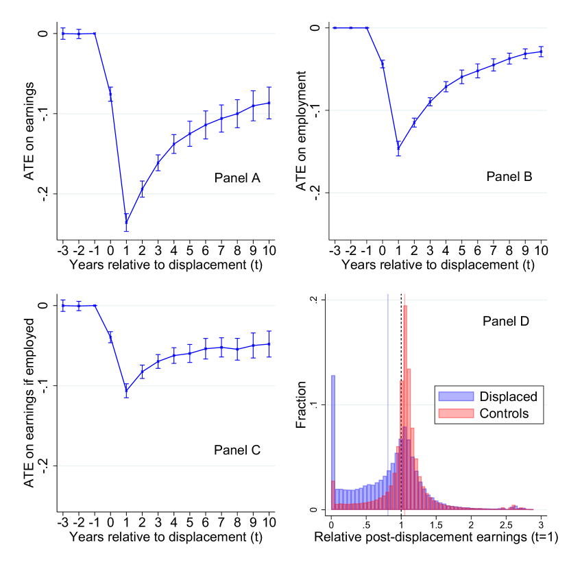
Figure 1: Average effects of displacement

Note: Panels A–C show estimated differences between displaced workers and matched controls (ATE) (with 95 percent confidence intervals). Panel A shows estimates for labor earnings (normalized by earnings in the year before displacement), Panel B for employment status, Panel C for labor earnings conditional on being employed. Standard errors clustered at establishment (pre-displacement) level. Panel D shows distributions of relative earnings in the year after displacement for the displaced and the matched controls. Solid lines indicate group means, the dashed line indicates unchanged nominal earnings.

4 Heterogeneous Treatment Effects

Our goal is to understand heterogeneity in displacement losses across different groups of workers. A conventional approach to study heterogeneity is to estimate linear interaction models. We start our analysis by estimating such models where our variables, one-by-one in separate regressions, are interacted with a displacement dummy.

Estimated interaction terms are reported in Figures 2 and 3. Dummies are kept as they are, whereas all other variables are standardized to mean 0 and standard deviation 1. The estimated interaction terms are, with few exceptions, statistically and economically significant as predictors of heterogeneous displacement effects. The continuous variables with the largest estimates (in absolute values) are age (older workers lose more), schooling (educated workers lose less), routine intensity (routine workers lose more), population density (workers in urban areas lose less), tenure (longer tenured workers lose more) and industry cycle (losses are smaller in growing industries). The dummy variables with the largest effects are the industry indicators for manufacturing (larger negative effects) and Education, industry and health (smaller effects in publicly funded industries). All of these estimates are in line with previous research, and broadly in line with the theoretical framework we outlined above. In some cases, different variables may plausibly capture the same causal processes (e.g., age and tenure), but in other cases it is more likely that the causes are different (e.g., age and publicly funded industries).

A key challenge is how to make sense of so many separate dimensions of heterogeneity. Furthermore, the underlying heterogeneity may be even more complex since these estimates ignores the potential for higher order interactions and non-linearities. We could gradually make the linear model richer by introducing more interaction terms and higher order interactions in the same model, perhaps relying on LASSO to avoid replicating spurious patterns in the data. But we choose to move straight to the GRF, which is ideal for our purposes as it is designed to handle settings with complex treatment-effect heterogeneity without imposing specific parametric functional forms. Furthermore, the GRF works well in settings where clustering is important.

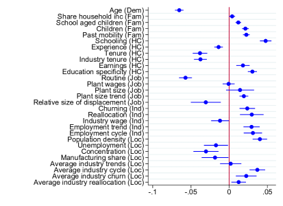
Figure 2: Displacement effects interacted with standardized continuous variables

Note: Regression coefficients from separate regressions, one for each variable. Outcome is labor earnings in the year after displacement normalized by earnings in the year before displacement. Explanatory variables are an indicator for displacement, the specific variable (standardized), and the interaction of the two. The graph displays the estimated interaction terms with 95 percent confidence intervals. Standard errors are clustered at the (pre-displacement) establishment level.

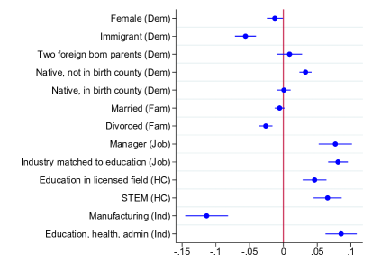
Figure 3: Displacement effects interacted with dummy variables

Note: Regression coefficients from separate regressions, one for each variable. Outcome is labor earnings in the year after displacement normalized by earnings in the year before displacement. Explanatory variables are an indicator for displacement, the specific (dummy) variable, and the interaction of the two. The graph displays the estimated interaction terms with 95 percent confidence intervals. Standard errors are clustered at the (pre-displacement) establishment level.

4.1 The GRF

To study multidimensional treatment-effect heterogeneity in a flexible way, we rely on the GRF developed by Athey et al. (2019). The forest iterates across random subsets of data, estimating a causal tree (Athey and Imbens, 2016) in each subset. Each causal tree is a sequence of splits. Each split partitions the data using one of the $x$ variables. The algorithm chooses the variable and cutoff value which maximize the difference in treatment effects between those on either side of the split. After each split, the data in the resulting nodes is split again until the observations have been grouped into leaves with similar treatment effects. To avoid overfitting, the tree is constructed using part of the selected subset, while treatment effects in each leaf are estimated using the other part. The estimates from a single tree can be non-robust and the GRF therefore computes many trees, with each tree using a random subset of observations and a random subset of $x$ variables. The complete forest is based on an ensemble of the estimated trees, ensuring that estimates are robust across subsamples, and providing consistent treatment-effect estimates.

The GRF is well-suited for our application. It allows us to consider heterogeneity across a large number of covariates within a unified model while minimizing the risk of overfitting. It can flexibly account for nonlinear effects and high-order interactions (e.g., between industry-specific human capital and industry trends). We use the covariates described in Section 3.2 and estimate the forest on annual earnings in the year $t+1$ after displacement. As we show below, this short-run heterogeneity translates into long-run earnings differences as well.

All steps of the estimation are clustered at the establishment level, which is important for avoiding dependencies across sub-samples which could lead to overfitting if outcomes are similar for workers who were displaced in the same event. We set aside a test dataset containing 20% of the closing establishments and their associated matched controls for use in the final targeting exercises in Section 7. The remaining 80% of the data is divided into 5 folds, containing an equal share of closing establishments and matched controls. We then leave one fold of the data out at a time and estimate a GRF on the remaining folds. The GRF gives us estimates of the conditional average treatment effects (CATE), but we only retain estimates for observations in the left-out fold. As a consequence, we do not use any information from the observation’s own establishment closure when estimating that observation’s CATE.

4.2 GRF Estimates of Heterogeneous Effects

Figure 4A shows our distribution of CATE estimates. As is evident, the conditional treatment effects have a very wide distribution around the average treatment effect (the vertical line). All estimates are negative, which means that the GRF predicts that all types of observations, as defined by our data, suffer from average earnings losses if their firm closes down. But how large these earnings losses are vary across types of observations. The distribution is skewed to the right, suggesting that many workers cope reasonably well, whereas a long left tail contains workers who are predicted to suffer very large earnings losses.

Figure 4B sorts observations into decile groups based on their estimated CATEs, with the hardest-hit workers in Decile 1. Within each decile, we calculate the Average Treatment Effect (ATE) as the difference in outcomes between treated and controls (by design, with similar values of $x$). By splitting observations according to their ranked CATE, we get groups with monotonically improving ATEs. The differences in effects are very large. Displaced workers in the least-affected decile (Decile $10$) lose only $5.9$ percent of their earnings on average. These small effects are (nearly) consistent with a fully competitive labor market without unemployment or job-specific wages. On such a market, job loss should leave earnings completely unaffected. In contrast, losses for workers in Decile $1$ amounting to a staggering $46$ percent of earnings. These effects, which are almost $8$ times larger than in Decile $10$, suggest that labor market imperfections are very prominent for workers in Decile $1$.

The relationship between ATE and CATE implies that the GRF captures heterogeneous effects out-of-sample. Figure 4B also allows us to compare the average CATE to the average ATE within each decile as a measure of how well-calibrated the GRF is. The ranking is identical and the average CATE is similar to the average ATE, but the variation is larger in the actual data (the ATEs) than predicted by the GRF (the CATEs). The GRF thus manages to accurately rank observations across deciles, but underestimates the quantitative differences across these ranks. This pattern caries over to other cuts of the data based on CATE as analyzed below, and we therefore focus on the ATE estimates whenever we discuss magnitudes. Figure 4B also plots doubly robust Agumented Inverse-Probability Weighted (AIPW) estimates which use GRF predictions of treatment propensity and the outcome. The small differences between the AIPW estimates and the unadjusted ATE estimates suggest that our basic matching procedure is sufficient, and we therefore primarily rely on the unadjusted ATE estimates in the remainder of the paper.

Before proceeding, the appendix deals with two pressing concerns regarding the validity of the overall identification strategy: the potential for spillover effects on the control group from large closures and the fear that early leavers from firms in gradual decay may affect the results. We show in Appendix figure LABEL:Appfig3_Robustness, that the distributions looks very similar when excluding closures with more than 20 workers, or when zooming in on closures where the change in net employment was less than 10 percent in the year prior to the event.

5 Effect Heterogeneity and Other Economic Outcomes

The results of Panels A and B in Figure 4 focused on the earnings effects one year after job loss. The massive heterogeneity we find in this dimension is striking. But we can use our estimates to analyse whether workers with large one-year displacement losses also suffer from other adverse economic outcomes.

Panels C and D of Figure 4 relate the displacement loss deciles to the estimated risk of displacement (using the estimated displacement propensity discussed in Section 3). Panel C plots the average risk by CATE decile after normalising the risk to $1$ in CATE Decile $1$. The relationship is monotonically negative and differences across deciles are substantial; the most resilient workers (in terms of earnings CATE) have a 40 percent lower estimated risk of displacement relative to the least resilient decile. As shown in Panel D, this pattern arises because workers with a high risk of displacement are heavily over-represented in the very lowest part of the CATE distribution; those with very large negative effects of displacement also experience a higher risk of displacement.

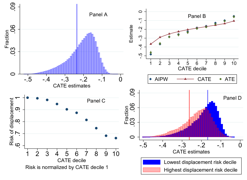
Figure 4: CATE, ATE, and the risk of displacement

Note: CATE:s for the main data set estimated using 5-folds estimation. Ranking of CATE:s is made for each fold separately. Panel A shows a histogram of CATE:s (line shows the estimated ATE for our sample). Panel B shows the CATE:s, ATE:s and doubly robust estimates (average AIPW scores) in the respective CATE deciles. For the ATE:s, we report point estimates and 95 percent confidence interval with standard errors clustered at the establishment level. Panel B shows the underlying earnings trajectories for displaced and matched controls within each decile group. Panel C shows the average estimated propensity to be displaced by decile of CATE:s. Scores are normalized relative to CATE decile 1 to highlight the relative risk. Propensity scores are estimated by logit on the full sample of workers. Panel D shows the distributions of CATE estimates separately for the lowest and highest decile of displacement propensity. Lines depict estimated ATEs from displacement in the two samples.

Figure 5 shows how the effects of displacement evolve over time for workers across the distribution of CATEs. Panel A plots ATEs over time for CATE deciles $1$ (least resilient) and $10$ (most resilient) as well as for the $10$ percent of observations straddling the median. Short-run CATEs are strongly predictive of displacement losses throughout most of our $10$-year follow-up period. After $5$ years, the earnings effects in Decile $1$ are six times larger that in Decile $10$, as compared to eight times larger in the first post-displacement year. Aggregating across the 10 years, the worst-affected decile is estimated to lose labour income corresponding to 2.43 years of pre-displacement labor earnings. This is almost exactly five times more than the losses of the least affected decile (0.48).

Panels B to D show outcomes over time relative to the event separately for the treated and controls. As the controls provide the counterfactual outcome for the treated, the differences between these series are identical to the ATEs. We show the series separately for the top and bottom deciles as well as the median group. Annual earnings are normalized relative to the median CATE group in $t-1$ to highlight pre-existing earnings differences. Reassuringly, pre-trends are perfectly matched within each of the deciles even though they differ across deciles. A priori, we could have expected workers with a more positive counterfactual trajectory to suffer larger effects since they have more to lose, but the results point in the very opposite direction. The large effects for low-decile workers arise because of poorer outcomes for the treated, not because of better outcomes among controls. Observations in Decile $1$ already had lower earnings than the median before displacement and a much less favorable counterfactual (non-displaced, control) earnings trajectory. Decile $10$, on the other hand, experiences smaller effects, but also above-median pre-displacement earnings and more positive counterfactual earnings trajectories. Figure LABEL:f:emp_potential in the appendix replicates Figure 5 with employment as the outcome. The results are very similar, which highlights the importance of the employment margin.

The results of Figures 4 and 5 jointly suggest that job loss episodes lead to accelerated gross-earnings inequality by causing larger earnings losses for workers who already had lower wages from before the event, who would have had worse earnings trajectories without displacement, and who have a higher risk of displacement. Public support systems however mitigate the pass-through from gross labor earnings to after-tax income by means of transfer systems such as unemployment insurance and social assistance, and through progressive taxation. The degree of insurance is mechanically the largest for workers who experience large gross-earnings losses. In addition, as outlined in our theoretical framework, workers could experience larger earnings losses because they are well-insured in case of unemployment. Both of these channels suggest that the degree of insurance should be positively correlated with the size of the earnings effect. To illustrate this, we examine the impact on disposable income by labor-earnings CATE decile in Figure LABEL:fig4_dispinc. Disposable income losses are much smaller than labour income losses, in particular in Decile $1$ where the degree of implied insurance is $71$ percent (as compared to around $50$ percent in Deciles $6$ to $10$). Thus, insurance responses mitigate the impact on inequality, but instead shift parts of the financial burden from the most affected workers onto public finances.

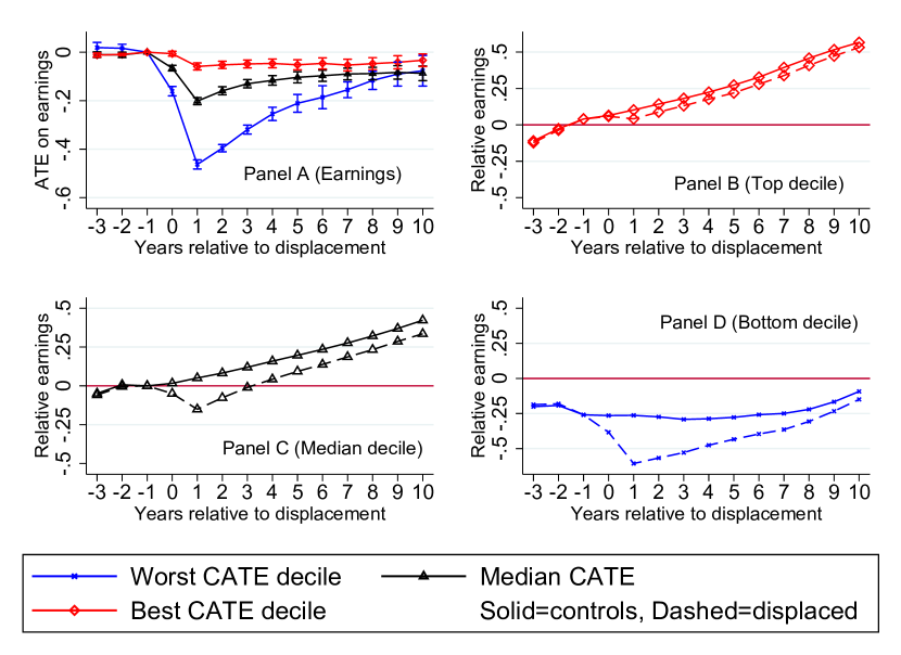
Figure 5: Effects of displacement across time and CATE deciles

Note: The figure shows statistics for three decile groups of the CATE distribution. The median group straddles the median (i.e. it contains the $10th$ and $11th$ ventile). Panel A shows ATE effect over time, similar to figure 1, but separately for the decile groups. Point estimates and 95 percent confidence interval with standard errors clustered at the establishment in $t=-1$. Panel B–D show the underlying earnings trajectories for displaced and matched controls within each decile group for the top, bottom and median deciles respectively. The series are normalized to reflect differences relative to the median group in $t=-1$.

6 Predictors of Heterogeneous Effects of Displacement

The purpose of this section is to highlight how worker characteristics and aggregate conditions are related to magnitudes of the displacement losses. As in any study of treatment-effect heterogeneity across non-randomized attributes, we correlate attributes with estimated effects. The estimated earnings loss within each split of the data should be considered as an estimated causal effect of displacement for that worker group, but the splits themselves should not be given a causal interpretation.

Figure 6 displays differences in characteristics between workers in the lowest and highest quartiles of estimated CATE:s. Continuous variables, shown to the left, are standardized to mean zero and a standard deviation of unity. Dummies are reported at their true mean values to the right. Solid blue bars are sorted according to the magnitudes of the difference between the bottom and the top quartile. In Appendix B (Figure LABEL:fig_interdecile) we compare the top and bottom deciles instead, with similar (but starker) results.

The characteristics that stand out are the same as in the simple one-dimensional heterogeneity analysis. The quartile with the largest losses contains older workers with lower levels of schooling; these two variables stand out aas having the largest cross-quartile differences of all continuous variables. Human capital variables (e.g., tenure) and occupation related factors (e.g., job routineness) also differ markedly across the CATE distribution. More vulnerable workers also have less prior mobility and are less likely to hold an education in STEM fields. As already documented, vulnerable workers had lower earnings before becoming displaced. But, they seem to have more sector- and firm-specific human capital, as evidenced by their longer industry and job tenures. They are more concentrated in manufacturing industries and they are more exposed to unfavorable industry characteristics such as bad long-term industry trends and low churn rates. They are more likely to live in rural areas with high unemployment rates and high manufacturing shares. Their establishment’s closure also displaces a larger share of workers in their industry-location cell.

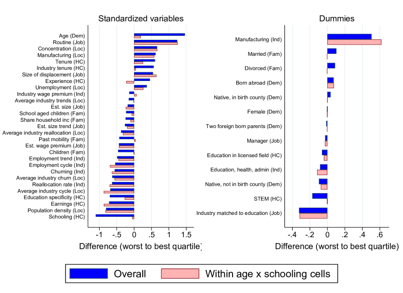
Figure 6: Differences in characteristics across CATE quartiles

Note: The figure shows differences in characteristics between the lowest and highest quartile of CATE:s, using the main data set. CATE:s estimated with 5-fold estimation and ranking done within each fold. The left-side panel include standardized (mean $0$ and standard deviation $1$) continuous variables and the right-side panel include dummy variables. Blue bars are for the overall quartiles and red bars cover the highest and lowest quartiles of CATE within each combination of 8 schooling and 10 age categories (see Figure 7 below).

6.1 Heterogeneity Across and Within Age and Years of Schooling

Age and years of schooling stand out as characteristics that differs substantially across quartiles in Figure 6. As these variables are likely to be correlated, they could, in principle, capture the same underlying factor(s). We therefore let Panel A of Figure 7 plot treatment-control differences (i.e. ATEs) estimated separately for $80$ combinations of age and schooling. As is evident from the figure, a higher age is associated with a larger ATE regardless of the level of schooling, and longer schooling is associated with a smaller ATE regardless of age. Young workers with at least a bachelor’s degree lose less than ten percent of their earnings, whereas old workers who have not completed high school suffer losses of over 40 percent. Panel B shows AIPW estimates instead, which adjusts for any imbalances related to X-variables within each cell, but as expected the results are almost identical to the ATEs. In the appendix (figure LABEL:Fig:AppCountourCATE), we show that the corresponding CATE estimates are similar, but less noisy.

In panels C and D we exploit GRF predictions within each of these $80$ age-schooling combinations. They show ATE estimates among the most (least) resilient CATE quartile within each combination. In (almost) all $80$ cases, the GRF identifies at least a quarter of workers with ATEs below the overall grand mean, and a quarter with ATEs above the overall grand mean. The worst-affected quartile (as identified by the GRF) of $30$ year-old university graduates has larger earnings losses than the least affected quartile of $55$-year old compulsory school graduates.

The red (shaded) bars of Figure 6 indicate how the GRF can find treatment-effect heterogeneity within age and schooling combinations. The bars show differences in means across CATE quartiles defined within age-schooling cells. Much of this within heterogeneity is related to industry and location characteristics. A more direct illustration of the importance of industry and location characteristics is shown in Figure LABEL:fig7_Extreme in the appendix; it illustrates a strong relationship to manufacturing intensity and population density for the extreme age-education groups of those younger than 30 with at least a bachelor’s degree and older than 50 with only 9 years of schooling.

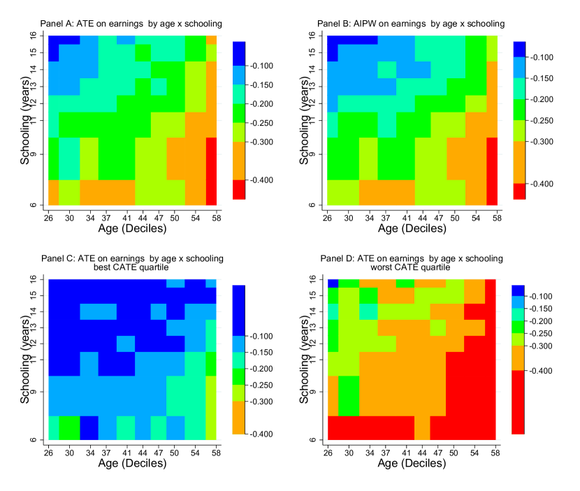
Figure 7: Displacement effects across and within combinations of age and schooling

Note: The figure divides training set workers into cells by age and schooling. Schooling has been aggregated to 8 groups by pooling the few with 10 years of schooling together with those with 9 years of schooling, and by letting the top group include all with 16 or more years of schooling. Age is defined in deciles among the displaced and the x-axis shows the median in each age group. Colors indicate the size of point estimates. Panel A shows estimated ATE:s by combinations of age and schooling. Panel B shows AIPW estimates separately within each of the 80 groups. Panel C replicates panel A, but only uses the highest quartile of 5-fold CATE:s within each group. Panel D repeats the exercise for the lowest quartile.

6.2 Heterogeneity Across and Within Establishments

We have performed two different exercises to assess the importance of establishments for our estimated heterogeneous earnings effects. We first note that CATE estimates should be highly correlated across coworkers from the same event if establishment-specific factors are important. In the appendix (figure LABEL:Appfig_within), we show that about half of the variation in CATE across displaced individuals is shared with displaced coworkers, while the other half is specific to individuals within the same event. For our second exercise, we divide the sample by CATE decile within each establishment and estimate the ATE by within-establishment decile. As a comparison, we compute average CATE estimates for each closing establishment (using only the CATEs of coworkers). We then divide the sample into deciles of these establishment-level CATEs and estimate the ATE for each (across-establishment) decile. Results are shown in Figure 8A (within heterogeneity) and 8B (across heterogeneity). To ensure comparability, we focus on events with at least 10 displaced workers in both of these panels. The amount of heterogeneity documented in panel A is very similar to panel B, which indicates that there is about as much heterogeneity within as across establishments.

Establishment-level CATEs (used in panel B) will be a good predictor of treatment effects if either establishment-level variables (the wage premium, size, size trend,..) are important, or if important individual/job-level variables are correlated within establishment (sorting), or if market-level factors matter (since industry and location are fixed within event). On the other hand, any remaining CATE differences between workers displaced from the same establishment (panel A) must be attributed to individual-level factors that vary within establishments. In Panels C and D of Figure 8, we show that much of the variation in effects across establishments can be approximated by variation across markets, where a market is defined as industry times location and year. When characterizing markets, we use the average CATE among workers who are displaced in other events in the same market. Results for splits by market CATE are shown in panel C. The exercise forces us to exclude singleton events, i.e. events where just one establishment is closed down in a market, and to facilitate a fair comparison we recalculate the across-establishment estimates for this sample in panel D. The results show that we can recover a substantial part of the heterogeneity across events by ranking observations by the CATEs of other events on the same market. In the appendix (figure LABEL:Appfig_within), we show that about half of the variation in CATEs across establishments can be approximated by (leave-out) market CATE.

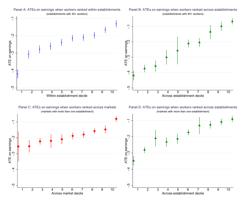
Figure 8: Displacement effects across and within establishments

Note: Panel A shows ATE estimates when displaced workers are ranked based on their within-establishment CATE. Panel B shows ATE estimates when displaced workers are ranked based on the CATE of their co-workers (defined as the leave-out mean for the workers at the establishment and then averaging over the individuals in the CATE decile.) Panels A and B exclude establishments with fewer than 10 displaced workers. Panel C ranks the workers by the average CATE in their market (location-industry cell). Only markets with at least two establishment closures are included in panel C. Panel D ranks workers by the CATE of their co-workers like Panel B, but only includes markets with at least two establishment closures. Control workers are allocated to the same sample as the displaced worker they were matched to in all panels.

6.3 Partial Effects of Location and Industry Conditions

As we showed above, much of the heterogeneity within age and education combinations is related to local labor markets or industries. Similarly, much of the across-establishment variation can be approximated by market-level factors. This is potentially important from a policy perspective since policymakers are more likely to use place-based or industry-related policies than policies targeting establishments based on their idiosyncratic characteristics. We therefore aim to describe the most important industry and location variables in more detail. Isolating the importance of market-level factors is not trivial since workers are likely to be sorted across regions and industries. For that reason we use the GRF to estimate partial dependence functions, holding the individual characteristics at their empirical levels and sequentially rotating across all observed sets of market characteristics within the same year. This way, we capture the predicted role of aggregate conditions across the full distribution of displaced workers, making full use of the GRF’s non-linear nature. Because market-level factors are correlated, we will split locations and industries into groups, and then characterize the attributes of these groups.

Formally, we divide the vector of characteristics $X$ into parts related to the location ($X^{L}$), the industry ($X^{S}$), or the displaced worker and lost job ($X^{I}$). Worker $i$ was displaced from location $l(i)$ and industry $s(i)$, with $X_{l(i)}^{L}$ and $X_{s(i)}^{S}$ being the corresponding location and industry characteristics. Then we compute:

$$\tau_{l}^{L}=\frac{1}{N}\sum_{i=1}^{N}\text{CATE}(X^{L}=X_{l}^{L},X_{s(i)}^{S},X_{i}^{I}),\quad\tau_{s}^{S}=\frac{1}{N}\sum_{i=1}^{N}\text{CATE}(X_{l(i)}^{L},X^{S}=X_{s}^{S},X_{i}^{I}),$$ (4)

where $\tau_{l}^{L}$ and $\tau_{s}^{S}$ is the GRF’s prediction of average displacement effects if all workers experienced the conditions in location $l$ or industry $s$. $N$ is the number workers in the sample. We use these predictions to rank industries and locations, and to derive interquartile differences in terms of $X^{L}$ and $X^{S}$.

Further, we classify workers based on their individual characteristics using a similar strategy. To this end, we hold worker characteristics fixed and combine them with each observed combination of location and industry conditions. Then for each worker $i$ we compute:

$$\tau_{i}^{I}=\frac{1}{N^{L}\times N^{S}}\sum_{l=1}^{N^{L}}\sum_{s=1}^{N^{S}}\text{CATE}(X_{l}^{L},X_{s}^{S},X_{i}^{I}),$$ (5)

where $N^{L}$ and $N^{S}$ are the number of locations and industries respectively. $\tau_{i}^{I}$ only reflects worker-level characteristics since we average over the same set of location and industry conditions for all workers (by year).

6.3.1 ATE Estimates by Partial Market and Worker Quartiles

Table 1 shows estimated ATEs for different cuts of the data building on combinations of $\tau_{l}^{L}$, $\tau_{s}^{S}$ and $\tau_{i}^{I}$. Panel A shows estimates for the lowest (Column 1) and highest (Column 2) quartile of worker-level effects ($\tau_{i}^{I}$). Column 3 shows the inter-quartile differences with associated standard errors in Column 4. The top row shows that workers in the lowest quartile of $\tau_{i}^{I}$ experience $26$ pp larger losses than the top quartile. In the rows below, we zoom in on workers exposed to different combinations of location and industry conditions and we see significant differences in ATEs across worker types even within each set of market conditions (ranging from $30$ pp to $16$ pp). Market conditions are particularly important as predictors of earnings losses for workers with poor individual characteristics. The ATEs vary nearly as much when comparing across market (industry and location) conditions for the lowest worker quartile ($25$ pp difference, comparing across rows) as when comparing across worker quartiles within the worst market (industry and location) quartile setting ($30$ pp).

In Panels B and C, the columns instead represent location and industry (defined at the 3-digit level) quartiles, respectively. Here, the different rows represent worker types. Panel B shows that the quality of the location matters for the size of the displacement effect even when holding the worker quartile ($\tau_{i}^{I}$) fixed (interquartile differences are $6$ to $12$ pp depending on type). Workers also suffer significantly larger effects if displaced from bad industries (Panel D), in particular if they belong to the bottom worker quartile. In this group, estimated losses are $19$ percentage points larger if displaced in a low-quartile industry as compared to a high-quartile industry.

Market conditions should, in general, matter more if workers are immobile and we therefore estimate how displacement events affect mobility across locations and industries. Panels D shows that workers are more likely to change location if displaced under worse conditions. The estimated effects on location mobility are small, partly because location mobility overall is very low, but the results show that this is true even for workers displaced in very bad locations. The results also indicate that job loss leads to more mobility across locations among workers who are more resilient.

Panel E shows that workers are more likely to move away from their (1-digit) industry if they are displaced from an industry with large displacement effects – the magnitudes here are much more substantial than for location mobility. But the fact that industry characteristics in general correlate so strongly with displacement effects suggests that the degree of industry mobility is insufficient to offset the negative effects of being displaced from a bad industry.

Table 1: Earnings and mobility effects, by partial market and worker characteristics

	(1)	(2)	(3)	(4)
	Worst	Best	Interquartile	Standard Error
	Quartile	Quartile	Difference	of Difference
Earnings Estimates
Panel A: Worker Quartiles, earnings effects
All Market types	-0.370	-0.114	-0.256	0.008
Worst Market quartiles	-0.502	-0.200	-0.302	0.090
Median Markets	-0.361	-0.149	-0.211	0.026
Best Market quartiles	-0.254	-0.093	-0.162	0.019
Panel B: Location Quartiles, earnings effects
All worker types	-0.298	-0.179	-0.119	0.016
Worst worker quartile	-0.424	-0.306	-0.118	0.012
Median workers	-0.262	-0.179	-0.083	0.017
Best worker quartile	-0.158	-0.100	-0.059	0.029
Panel C: Industry Quartiles, earnings effects
All worker types	-0.330	-0.180	-0.150	0.020
Worst worker quartile	-0.463	-0.274	-0.188	0.022
Median workers	-0.286	-0.183	-0.102	0.020
Best worker quartile	-0.152	-0.102	-0.049	0.037
Mobility Estimates
Panel D: Location quartiles, effects on location mobility
All worker types	0.017	0.005	0.012	0.002
Worst worker quartile	0.011	0.011	0.000	0.002
Median workers	0.020	0.003	0.017	0.004
Best worker quartile	0.022	0.003	0.019	0.006
Panel E: Industry quartiles, effects on industry mobility
All worker types	0.332	0.225	0.107	0.027
Worst worker quartile	0.411	0.254	0.158	0.029
Median workers	0.309	0.242	0.067	0.026
Best worker quartile	0.239	0.183	0.056	0.047
Note: Panel A–C display displacement effects on earnings on year after displacements (calculated as displaced-control differences, ”ATEs”). Panel A shows earnings estimates for the worst quartile of workers (Column 1) and the best quartile (Column 2), using the worker resiliency measure described above. Results for workers in all markets (interaction between industry and location), for workers in the worst (best) market quartiles, and for median markets (workers in the 3d or 4th market quintiles). Column 3–4 show the difference between Columns (1) and (2), and the standard error for the difference (clustered at the pre-displacement establishment level. Panels B show earnings estimates for the best and the worst quartiles of locations using the partial-effects procedure described above. Panel C shows similar earnings measures when dividing by the best and worst industries. Both Panel B and C report estimates for all workers and when dividing workers by worker resiliency using the worker resiliency measures described above. Median workers are those in the 3d or 4th worker quintiles. Panel D shows displacement effects on location mobility (mobility defined as moving to another local labor market between one year before and three years after the displacement), and Panel E displacement effects on industry mobility (mobility defined as switching 1-digit industry between one year before and three years after the displacement). Panels D–E show results for the full sample of workers and when dividing the sample by worker resiliencey as in Panels B–C. Standard errors in Panel B and D clustered at the location level, and standard errors in Panel C and E clustered at the industry level. All estimates use the main data set. Rankings of workers and reshuffling done using the k-folds procedure.

6.3.2 Characteristics of Markets with Large Partial Effects

Table 2 describes the best and worst locations and industries (top and bottom quartiles of $\tau_{l}^{L}$ and $\tau_{s}^{S}$). Panel A shows location characteristics ($X^{L}$) for the good and bad locations as well as cross-quartile differences in $X^{L}$. Standard errors for differences are clustered at the location level. Locations with bottom-quartile partial effects ($\tau_{l}^{L}$) are in particular characterized by much lower population density. These locations also have high unemployment rates and a more concentrated industry structure dominated by declining industries and manufacturing jobs.

Panel B shows similar results for industry characteristics. Industries with large predicted earnings losses for the average worker ($\tau_{s}^{S}$) are exclusively found in manufacturing, while industries with small predicted losses are in non-manufacturing sectors. Industries with very negative $\tau_{s}^{S}$-estimates also have higher wage premia, are less dynamic (lower churning and reallocation rates), and experience declining employment trends over both the short and the long run. All of these attributes are typical of manufacturing, but they are also related to effect heterogeneity if we only compare different manufacturing industries to each other, or if we only compare non-manufacturing industries to each other (see Table LABEL:t:manuf in the appendix).

Table 2: Location and industry characteristics for the worst and best locations/industries

	(1)	(2)	(3)	(4)
	Worst Quartile	Best Quartile	Interquartile Difference	Standard Error of Difference
Panel A: Location characteristics, by location quartiles
Population density	20.410	147.913	-127.503	3.026
Unemployment rate	0.105	0.062	0.043	0.003
Industry concentration (HHI)	0.040	0.025	0.015	0.001
Share manufacturing	0.230	0.106	0.124	0.016
Average industry trend	0.058	0.113	-0.055	0.005
Average industry cycle	0.005	0.011	-0.006	0.001
Average industry churn	0.203	0.268	-0.065	0.004
Average industry reallocation	0.144	0.161	-0.017	0.002
Panel B: Industry characteristics, by industry quartiles
Employment trend	-0.150	0.215	-0.366	0.061
Employment cycle	-0.033	0.024	-0.057	0.006
Industry wage premium	0.067	-0.049	0.116	0.027
Churning	0.177	0.253	-0.076	0.021
Reallocation rate	0.116	0.164	-0.048	0.008
Manufacturing	1.000	0.000	1.000	0.000
Education, health, admin	0.000	0.240	-0.240	0.113
Note: Panel A displays average location characteristics for the best and the worst quartiles of locations, and Panel B displays average industry characteristics for the best and the worst quartiles of industries. Both panels use the partial-effects procedure described above. The location and industry characteristics are described in Section 3.2. Standard errors in Panel A clustered at the location level, and standard errors in Panel B clustered at the industry level. All estimates use the main data set.

In the appendix (Table LABEL:t:worker_stats) we describe the characteristics of the top and bottom partial worker-level quartiles ($\tau_{i}^{I}$) and compare these to differences across raw CATE quartiles. Overall, the results show relatively small differences between the partial and overall quartiles. This suggests that a very small share of the differences in treatment effects associated with worker characteristics arises because of correlations with market factors. The table reaffirms the strong relationships with age, schooling, and specific human capital. The most striking difference is related to gender. Females are highly over-represented in the lowest partial quartile ($\tau_{i}^{I}$), despite not being in the lowest overall CATE quartile. The reason is that females are underrepresented in manufacturing where effects tend to be larger. There are also fewer immigrants in the best partial quartile than in the best overall CATE quartile, reflecting both an under-representation of immigrants in manufacturing and an over-representation of immigrants in metropolitan areas where effects tend to be more muted. Similarly, an over-representation of STEM graduates in the most resilient partial quartile reflects that many engineers work in manufacturing, but suffer much smaller effects than other workers from these industries who lose their jobs.

7 Policy Targeting

Given the well-known severe average impact of displacement, policymakers have designed various forms of policies to ameliorate the consequences of job loss, or even to prevent it from occurring (e.g. through short-time work schemes or employment protection legislation). But supporting all groups of workers equally may be misguided, as some groups of workers suffer only very small losses. As shown by our analysis above, targeting based on a single variable is unlikely to capture the complex heterogeneity pattern uncovered by the GRF. But for policy purposes we would like to find usable (i.e. simplified) targeting principles that would direct policymakers toward the right set of workers. One problem is that we have a very large number of possible combinations of variables to choose from (in particular, if variables are continuous).

As a first step, we consider key one-dimensional predictors at the worker level (age, schooling), industry level (manufacturing) and location level (population density), and pairwise combinations of these. To make further progress, we then select targeting variables using optimal policy trees (Athey and Wager, 2021). We consider trees of depth two, selecting the two best targeting variables from our full set of variables. Each set of variables defines a targeting rule which we use to extract a fraction of targeted observations (varied between 5 and 25 percent of the overall sample) and estimate the displacement effects on earnings one year after displacement (ATEs) for the selected group of workers. For targeting using the full GRF, this implies selecting the workers with the most negative CATEs, for age it means selecting the oldest workers, and so forth. To obtain a fair comparison between the GRF and the simple targeting rules we use our held-out test set, i.e. 20 percent of the closing establishments and their matched controls not used for producing any of the results shown so far.

The results are reported in Figure 9. The blue lines in all panels show the displacement effect among a randomly selected set of workers. This results in an average earnings loss of 24.6 percent regardless of how many workers we select. On the other extreme, when using the full GRF model, we find, as expected, a group of workers with much larger displacement effects, as shown by the red line. The five percent of workers who are hit the hardest according to the GRF experience displacement losses of 54 percent. Among the hardest-hit 25 percent, earnings losses are 41 percent. Panel A also includes targeting based on age (target the oldest first) and schooling (target the least educated first). The green line shows that average earnings losses are 42 percent among the oldest five percent of workers, and 34 percent among the oldest 25 percent. Targeting based on schooling, shown by the orange line, reaches workers who are on average less hard-hit than the oldest workers (e.g., losses of 40 percent when targeting the five percent least educated). In both cases, targeting is substantially better than random, but clearly worse than targeting based on the output of the GRF.

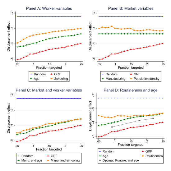
Figure 9: Displacement effects on earnings for workers selected by different targeting policies

Note: The figure reports estimated observed displacement effects on earnings one year after displacement (calculated as displaced-control differences, ”ATEs”) when selecting a fraction of the workers using different targeting rules. The random rules selects a random set of workers. The GRF selects workers using the estimated CATEs. Panel A: the age rule targets the oldest workers first and the schooling rule the least educated first. Panel B: the manufacturing rules targets a random set of manufacturing workers, and the populations density selects workers in the least dense locations first. Panel C targets the oldest respectively the least educated manufacturing workers. Panel D reports targeting results when targeting the oldest workers (age) and workers in the most routine occupations. It also reports results when targeting on both age and routineness using optimal policy rules (Athey and Wager, 2021).

Panel B of Figure 9 considers targeting on industry and location characteristics. If manufacturing workers are selected at random, the losses of the workers reached by the policy are around 36 percent (green line). Since manufacturing workers constitute more than 25 percent of our sample, this average loss is the same when targeting the worst 5 percent and the worst 25 percent. However, Panel C shows that it is possible to improve targeting by selecting the oldest or least educated manufacturing workers. The first five percent of individuals selected according to this rule suffer earnings losses of 48 percent; if a quarter of the individuals in the test sample are selected, their losses amount to 39 percent. Targeting workers in locations with low population density (shown by the orange line) does slightly less well in terms of identifying the hardest-hit individuals than targeting based on manufacturing (see Panel B).

In Panel D, we explore targeting rules based on optimal policy trees (Athey and Wager, 2021). Specifically, we assume that we have a fixed per-person cost of the policy and that the benefits of the policy are proportional to the income losses of displacement. We consider different costs of the policy in order to generate different fractions of treated/targeted (the figure shows the implied targeting from three optimal policy trees, assuming different costs of the policy). It leads to targeting based on age and the routine content of the job. For a policy cost that results in about 10 percent treated, the optimal policy is to target everyone older than 59 years, and to target workers aged 51–58 years if the level of routineness is above the 80th overall routineness percentile (corresponding to the 69th percentile in the sample of displaced workers). Most likely, age and routineness are selected because age captures losses related to occupation and establishment-specific human capital, and lost job-ladder related rents in the pre-displacement job, while routineness may capture exposure to both declining demand (e.g., related to the manufacturing industry) and low skills. The grey line in Panel D shows that using information on both routineness and age improves the targeting when compared with targeting on only age or only on routineness, but still performs worse than targeting on the entire GRF.

We conclude that the simple targeting policies give better results than randomization, but do not quite reach the performance of the GRF model. This confirms our key finding that the size of displacement losses cannot be explained by any single variable in isolation. The GRF’s ability to take many characteristics into account in a flexible way is necessary for correctly predicting how individuals fare following displacement. If GRF estimation based on all the characteristics we include is unfeasible, a targeting rule that combines information on routineness and age does best.

8 Conclusions

Our paper has demonstrated how characteristics of workers, establishments and markets interact to generate strongly heterogeneous earnings losses following job displacement. Our paper contributes to a vast literature which documents the severe earnings consequences of job loss. We show that groups with large negative effects are vulnerable in other economic dimensions as well; they have lower pre-displacement earnings, a larger propensity to be displaced, and much worse counterfactural earnings trajectories than other displaced workers. In the literature, many explanations for post-displacement losses have been put forward. These have highlighted factors such as firm, industry and occupation-specific human capital, location mobility and aggregate conditions. Our results confirm that determinants of earnings losses after displacement are multidimensional, as substantial systematic heterogeneity remains even after conditioning on crucial predictors such as age and schooling, or the identity of the closing establishment. While older workers with lower levels of general human capital lose more on average, even old and low-educated workers can do better than the average worker if other circumstances are favorable. Aggregate demand-side conditions at the local and industry level appear to play an important part in determining the size of losses as workers in urban areas and outside of manufacturing consistently fare better than other displaced workers. Our results show that the heterogeneity is too complex to be well-approximated by one-dimensional targeting rules. The targeting rule which comes closest to achieving the targeting recommended by the GRF is to focus on older workers in either manufacturing or routine occupations. This is a group which suffers from a combination of detrimental individual and market-level conditions.

At a more general level, our results indicate that the economic value of jobs is highly heterogeneous. Some groups of workers, primarily the young, well-educated and those who work in non-manufacturing industries, are able to move on to a new job with only short-lived and marginal losses if their firm closes down. This pattern is consistent with a fully competitive labor market without unemployment or job-specific wage rents. Other groups of workers, such as the older and less educated, instead suffer from very large and prolonged losses if their jobs disappear, suggesting that these workers are exposed to highly imperfect labor markets. The interaction between worker and market characteristics should also be understood in this context; workers with favorable individual characteristics have small effects of job loss regardless of market conditions, whereas workers with large average effects are much more sensitive to market conditions.

Appendix A Appendix A: Data Details

Below, we explain the variables used in the GRF model and when matching displaced workers to non-displaced controls.

A.1 Demographics

Data on basic demographics are drawn from the administrative population register Louise produced by Statistics Sweden. Data in Louise is collected in November of each year. Age is measured in years. We include a Female dummy. A categorical Native-immigrant variable takes the value zero for natives, one for those with two foreign-born parents, and two for those born abroad (unless both parents are born in Sweden).

A.2 Family

Civil status is coded using two dummies. $Married$ workers are either formally married, or cohabit with a partner with whom they have a common child. This definition is well in line with Swedish perceptions of ”marriages” and is used in most research on Swedish data. $Divorced$ is a dummy for workers whose marriage has ended and who are not currently defined as married according to $Married$.

To quantify the economic value of the partnership and degree of dependence, our Share of household income variable measures the subject’s labor earnings as a share of total household labor earnings.

We measure the number of children in the household using two different variables. Children contains the number of all children under the age of 18 in the household, whereas School-aged children counts children aged 7 to 17. We make this distinction to allow the second variable to measure the additional impediments to mobility that may arise when children start school at age 7.

Social ties to the current location are measured by two variables. First, we define a dummy for being Born outside of the current county. This variable naturally takes the value 1 for all foreign-born. We also measure Past mobility as the number of moves across local labor market boundaries during the past 10 years. This variable is a lagged counterpart of our key indicator for geographical mobility after the event.

A.3 General Human Capital

Years of schooling are based on the highest achieved level of education. Labor market experience is measured as the number of years employed during the 10 years prior to displacement. Because of the tenure restriction, all displaced and control workers must have been employed for at least three years prior to the year $t=0$ and the variable therefore has a range from 3 to 10.

In this category, we also include pre-displacement earnings. We measure these by Earnings as the rank among the full population of displaced and controls in year $t=-1$, as well as two variables capturing Earnings growth from $t=-3$ and $t=-2$ respectively to $t=-1$. The rank form of the Earnings variable has been chosen to ensure orthogonality to time trends.

A.4 Specific Human Capital

It is likely that workers differ in terms of how costly or difficult it is for them to switch firm and industry if hit by a negative shock. The ability to adjust along this margin is potentially determined by the degree to which the worker is tied to the closing firm or sector. In order to measure the empirical relevance of these aspects, we include variables capturing pre-closure establishment Tenure (truncated at 10), and the number of years spent in the same industry as the closing establishment (Industry tenure, also truncated at 10).

Furthermore, we characterize the Education specificity using data on the 1-digit level and 3-digit field of the highest achieved education (thus, high school programs and college majors). Our metric uses the fraction of workers, by education cell, that is employed in the ten main 3-digit industries. The strategy follows Altonji et al. (2012). Examples of fields with high levels of specificity are pharmacists and nurses.

We further include an indicator for $STEM$ education beyond high school. We also provide a dummy for Education in a licensed field, that is a field that caters to the health or education sector.

A.5 Lost Job Characteristics

The causal impact of job loss for displaced workers does not only depend on their outside opportunities, but also on aspects of the job that they have lost. We therefore define a number of variables which capture key characteristics of the lost job.

We first characterize the lost job by Plant size in terms of employment in $t=-1$, and Plant size trend between $t=-3$ and $t=-1$, measured as the difference in log(Plant size).

Additionally, we measure the Plant wage premium at the closing establishment. This feature is shown to be particularly important in the case of Austria by Gulyas and Pytka (2021). They study mass layoffs and characterize the affected firms by firm wage effects as estimated conditional on person-fixed effects in the tradition of the AKM model (Abowd et al., 1999). Indeed, there is a large literature discussing the origins of firm-specific rents, and how they should be estimated and interpreted (see, e.g., Card et al., 2018; Bonhomme et al., 2019; Lachowska et al., 2020, in the context of plant closures). A drawback of the AKM model is that it requires structural assumptions that we do not want to impose, and is likely to result in biased premium estimates for dying firms. We therefore take a slightly different route. As a reduced form measure of the pay level of the closing firm at the time of displacement, we use the leave-one-out mean of residual earnings in year $t=-1$ as in Card et al. (2013). For each displaced worker and potential control, we characterize the closing establishment environment by the average Mincer residual earnings of all co-workers at the same establishment. Residual earnings are computed using year-specific regressions of log earnings on 3-digit industry indicators, years of schooling, field of education (2 digits), gender, immigration status and a full set of age dummies.

We measure the Routine task component of the lost job. To this end, we use data on routine intensity by occupation from Autor and Dorn (2013) and Goos et al. (2014). We translate the occupational codes into the Swedish nomenclature. We have data on occupations for about half of our workers. We impute routine intensity for each worker based on the average routine score for those in the same detailed education-industry combination.

We further construct a Manager dummy for workers who are employed as managers. This information is drawn from the occupational codes, which we do not have for all workers, and therefore contains false negatives. To mitigate the problem, we impute manager status based on data from the previous three years if the information is missing in $t=-1$.

We calculate the Relative size of the displacement event as the share of total employment by 3-digit industry and local labor market combination. This is motivated by previous studies, e.g. Cederlöf (2019) and Gathmann et al. (2020), that have found that the impact of being displaced in a large event is particularly severe. One possible explanation for this finding is that workers from the same event may compete with each other for the same job openings, and this type of competition might be particularly problematic if the displacement event is large relative to the industry-specific local labor market.

Finally, we generate a variable for Industry being matched to education. This indicator takes on the value 1 for workers who were employed in one of the 10 main 3-digit industries for their 1-digit level and 3-digit field before displacement.

A.6 Industry Characteristics

There is ample evidence that, on average, workers have comparative advantage in their industry of employment and that shocks to this industry have an impact on their overall earnings prospects. Examples include Carlsson et al. (2016) for Sweden, who show that that technology shocks have a larger impact on workers’ wages if the shocks are shared with other firms in the same industry and that this distinction is entirely driven by workers with fields of education where most job-to-job mobility is within the industry. Similar arguments are made in Lamadon et al. (2019). It is also likely that displacement has more lasting negative effects in industries with low labor turnover such as manufacturing than in fluid sectors such as restaurants. Overall, this suggests that workers who lose their jobs in declining low-turnover sectors will suffer more adverse consequences, in particular if much of their human capital is industry-specific.

In order to quantify the conditions in each industry, we first construct time-consistent industry indicators at the 3-digit level. This is a non-trivial endeavour as the codes changed three times during our sample period. We start from the SNI2002 codes that our raw data provide for the period 2002 to 2010. Next, we rely on the SNI2002 code reported in 2010 and use it for all later years for those establishments that continue to exist beyond 2010, and conversely use the data from 2002 for establishments that existed prior to that. We refer to these overlapping establishments as stayers. We then use the modal overlap between SNI2002 (as imputed for stayers) and the current codes (SNI69, SNI92 and SNI2007) to fill in SNI2002 codes for non-stayers. This works particularly well for the years and sample we study, as almost all closing establishments existed in 2010 (due to the 3-year tenure requirement) and since most codes remained unchanged between SNI92 and SNI2002.

We measure Industry wage premia in each 3-digit industry as average earnings in the industry, residual on years of schooling, 2-digit education field, gender, immigrant background and a full set of age dummies. Furthermore, we also include average Churn and Reallocation rates for each industry. We follow conventions from Burgess et al. (2000), and define establishment-level churning as the number of workers who are hired or separated beyond what was needed for the actual change in employment between two adjacent years. The churning rate is measured as churning relative to the average employment during the two years. Similarly, we calculate excess reallocation in each industry as the excess creation and destruction of jobs over what was needed to adjust industry employment. The reallocation rate is measured relative to the average employment in the two years. We then aggregate the establishment-year churning rates and the industry-year reallocation rates to industry-level averages which are constant over time. When computing these numbers, we take care to exclude observations that satisfy the conditions for false closures as discussed above. Note also that the scale of the measures (relative to average employment in the two years) is in approximate percentages, but with a maximum of 2 and a minimum of -2.

We also follow the conventions from this literature when computing Employment growth over the past 10 years in each industry. Thus, for displacement events in the year $t=-1$, we define $Trend_{Ind,t}=(Emp_{Ind,t-1}-Emp_{Ind,t-10})/(Emp_{Ind,t-1}/2+Emp_{Ind,t-10}/2)$ which takes the value 2 for newly emerging industries and the value -2 for disappearing industries. This metric bounds cases where some very small industries experience extreme changes (including exits and entries) during the sample period. Similarly, we calculate the Industry-specific business cycle as the change in employment between year $t=-1$ and $t=0$ using the same metric.

We also add dummy variables for closures in the Manufacturing industry, as this industry has been a focus of the job displacement literature since Jacobson et al. (1993). Furthermore, we add a dummy for closures within Education, health and public administration, as the labor markets in these (mostly public sector) industries tend to experience a constant shortage of workers.

A.7 Location Characteristics

As with industries, there is ample evidence suggesting that local labor market conditions have causal effects on workers’ outcomes. This is also the case in Sweden, where wages seem to react to local labor market shocks (Carlsson et al., 2019).

Our local variables are measured at the level of local labor markets, which are an aggregation of municipalities. These are constructed by Statistics Sweden based on commuting patterns.

For each local labor market, we measure the Local unemployment rate as the number of residents who are registered with the public employment service (a prerequisite for receiving benefits from either the unemployment insurance system or from the municipal welfare system) divided by the size of the local labor force (sum of the registered unemployed and the number of employed as described above). Population density is also measured at the local labor market level. The Concentration of local employment across 3-digit industries is measured using an HHI index.

In addition, we measure local exposure to the industry characteristics discussed above. These shift-share/Bartík-style variables are calculated by multiplying each industry’s employment share in the local labor market (by year) with the characteristics of that industry and then summing over the industries within the local labor market. In this way, we define the Manufacturing employment share, Average long-term industry trend, Average industry business cycle, Average industry churn and Average industry reallocation.

It is important to note the fundamental difference between these variables and their industry-level counterparts. Whereas the industry-level variables measure characteristics in the industry from which the worker was displaced (and is potentially tied to, if changing industry is costly), the local labor market counterpart measure how exposed the worker is to these attributes if searching at random at the local labor market (which should be more pertinent for workers who are restricted in their mobility).

A.8 Aggregate Conditions

To capture aggregate conditions in the economy, which may both impact the average size of earnings losses, as well as have heterogeneous effects on different worker groups, we include the calendar Year ($t=0$) and the National unemployment rate in the year $t=1$. The national unemployment rate captures the aggregate business cycle conditions displaced workers experience after job loss. These have been shown to be an important correlate of earnings losses by Davis and von Wachter (2011).

Appendix B Additional Results

Table B.1: Sample statistics for displaced and non-displaced workers

	Controls	Displaced
	(1)	(2)
N workers	28,882,765	184,848
N establishments	230,613	21,794
Covariates
Demographics
Age

& 42.153 Female 0.478 0.347 Born abroad 0.097 0.130 Two foreign born parents 0.028 0.032 Native, not birth county 0.274 0.250 Family Married 0.644 0.587 Divorced 0.101 0.099 Children (# living at home) 0.780 0.745 School-aged children 0.524 0.466 Share household inc. 0.714 0.756 Past mobility (# location moves in last 10 years) 0.164 0.212 Human capital Schooling (years of education) 12.162 11.473

Experience (years employed in last 10 years) 9.229 8.910

Tenure 6.624 5.891

Industry tenure 7.922 7.127

Earnings (rank) 0.500 0.497

Earnings in t-2 0.994 1.014

Earnings in t-3 0.951 0.962

STEM education 0.097 0.109

Education in licensed field 0.238 0.071

Education specificity 0.565 0.470 Lost job characteristics

Establishment size 521.051 186.073

Establishment size trend 0.025 -0.024

Establishment wage premium 0.001 -0.033

Job routineness 0.515 0.558

Industry matched to education 0.560 0.375

Size of displacement 0.170 0.159

Manager 0.033 0.027

Industry characteristics

Employment trend 0.052 0.080

Employment cycle 0.005 -0.001

Industry wage premium 0.006 0.027

Churning 0.223 0.209

Reallocation rate 0.131 0.139

Manufacturing 0.230 0.367

Education, health, admin 0.383 0.079

Location characteristics

Population density 82.467 86.241

Unemployment 0.086 0.086

Concentration (HHI for industries) 0.031 0.031

Manufacturing (share of local emp.). 0.189 0.186

Average industry trends 0.081 0.079

Average industry cycle 0.007 0.007

Average industry churning 0.224 0.226

Average industry reallocation 0.147 0.149

Year 2005.881 2005.576

National unemployment 7.451 7.432     Note: Mean values of all covariates included in the analysis for the unmatched samples of displaced and controls. Married includes cohabiting couples with common children. Locations are defined as local labor markets for purposes of past mobility. Tenure and industry tenure are censored at 10 years. Industry tenure is defined based on 3-digit industries. Earnings rank is the earnings rank in $t-1$ in the full sample of displaced and non-displaced for that year. Earnings in $t-2$ and in $t-3$ are measured as percentages of the worker’s earnings in $t-1$. STEM education is defined as as having at least some post-secondary education in science/mathematics/IT or engineering/manufacturing. Education in a licensed field is defined as teacher training or health services education. Education specificity is defined as the employment share of the top ten 3-digit industries for those in the worker’s 3-digit educational field (top industries are field-specific). Establishment size is measured as the number of employed workers for whom the establishment was the main workplace during $t-1$. Establishment size trend is measured as the log employment change between $t-3$ and $t-1$. The establishment wage premium is leave-one-out mean wage conditional on demographics and education level and field. Job routineness is measured as the occupation’s intensity in routine manual and routine cognitive tasks as share of intensity in all tasks. Industry matched to education is defined as working in one of the top ten 3-digit industries for the 3-digit educational field. Size of displacement is measured as the closing establishment’s share of local 3-digit industry employment. Industry variables are measured at the 3-digit industry level. Employment cycle is measured as employment growth from $t-1$ to $t+3$ and trend as employment growth from $t-10$ to $t-1$. Wage premium is measured as residual wages in the industry, conditional on conditional on workers’ demographics and education level and field. Churning is measured as average gross separations/hires minus net employment growth at industry establishments; reallocation as average employment growth in industry establishments net of the industry’s growth rate. Location variables are measured at the local labor market level. Concentration is an HHI index for 3-digit industries. Employment cycles, trends, churning and reallocation are averages among the 3-digit industries in the location weighted by their local employment shares.

	Manufacturing			Non-manufacturing
	Worst Quartile	Best Quartile	Interquartile Difference	Worst Quartile	Best Quartile	Interquartile Difference
	(1)	(2)	(3)	(4)	(5)	(6)
Employment trend	-0.236	0.080	0.316	0.004	0.242	0.238
Employment cycle	-0.036	-0.007	0.030	-0.008	0.022	0.030
Industry wage	0.085	0.036	-0.049	0.090	-0.033	-0.123
Churning	0.179	0.160	-0.019	0.212	0.245	0.033
Reallocation rate	0.113	0.117	0.004	0.138	0.155	0.018
Manufacturing	1.000	1.000	0.000	0.000	0.000	0.000
Education, health, admin	0.000	0.000	0.000	0.004	0.375	0.370
Note: The table displays average industry characteristics for the best and the worst quartiles of manufacturing industries (Columns 1–3) and non-manufacturing industries (Columns 4–6). Both panels use the re-shuffling procedure described above. The industry characteristics are described in Section 3.2. Standard errors clustered at the industry level. All estimates use the main data set.

	Workers ranked by			Workers ranked by
	partial CATE			CATE
	(1)	(2)	(3)	(4)	(5)	(6)
	Worst Worker Quartile	Best Worker Quartile	Difference [1]-[2]	Worst Worker Quartile	Best Worker Quartile	Difference [1]-[2]
Demographics
Age	52.448	35.286	17.162	50.728	35.900	14.827
Female	0.403	0.314	0.089	0.366	0.366	0.000
Born abroad	0.168	0.057	0.111	0.163	0.091	0.072
Two foreign born parents	0.024	0.033	-0.009	0.025	0.037	-0.012
Native, not in birth country	0.215	0.307	-0.092	0.201	0.297	-0.096
Family
Married	0.637	0.539	0.097	0.629	0.526	0.103
Divorced	0.162	0.045	0.116	0.146	0.058	0.088
Children	0.317	0.916	-0.599	0.394	0.864	-0.470
School-aged children	0.235	0.492	-0.257	0.287	0.475	-0.188
Share houshold inc.	0.716	0.798	-0.081	0.724	0.788	-0.064
Past mobility	0.089	0.360	-0.271	0.101	0.344	-0.244
Human capital
Schooling (years of education)	10.073	12.986	-2.913	10.094	12.704	-2.611
Experience	9.381	8.578	0.803	9.341	8.510	0.831
Tenure	6.676	5.220	1.456	6.763	5.172	1.590
Industry tenure	7.926	6.456	1.470	7.946	6.445	1.501
Earnings (rank)	0.364	0.646	-0.282	0.377	0.587	-0.210
STEM education	0.031	0.254	-0.224	0.032	0.203	-0.172
Education in licensed field	0.058	0.088	-0.031	0.044	0.106	-0.062
Education specificity	0.428	0.528	-0.100	0.420	0.528	-0.108
Note: The table shows average worker characteristics differ for the best and worst quartiles of workers. Columns 1–3 rank workers by CATE and Columns 4–6 by the partial worker resiliency measure described above. Columns 2–3 and 4–5 display averages within the respective quartiles. Column (3) shows differences between Columns (1) and (2). The worker characteristics are described in Section 3.2. All sample statistics are for the main data set. Rankings of workers and reshuffling done using the k-folds procedure.

	Qini coefficient (x100)	SE (x100)
GRF	-3.95	0.3
Age	-2.06	0.2
Schooling	-1.66	0.2
Manufacturing	-1.51	0.2
Population density	-1.35	0.2
Manufacturing & age	-2.58	0.2
Manufacturing & schooling	-2.23	0.3
Note: GRF: workers with the lowest estimated CATEs; Age: oldest workers; Schooling: Manufacturing: manufacturing workers at random and then other workers; Population density: least dense locations; Manufacturing and age: oldest manufacturing workers; Manufacturing and schooling: least educated manufacturing workers.

Note: Panel A and C show calibration results, i.e. how the estimated CATE:s relate to ATE:s and doubly robust estimates (average AIPW-scores) in the respective deciles in sub-samples with less than 20 workers (Panel A) and with less than 10 percent change in employment between t-2 and t-1 (Panel C), similar to Figure 4B in the paper. Panel B and D show distributions of relative earnings in $t=1$ for displaced and matched controls in sub-samples with less than 20 workers (Panel B) and with less than 10 percent change in employment between t-3 and t-1 (Panel D), similar to Figure 1B in the paper. Solid lines are for the respective means, dashed lines indicate unchanged nominal earnings.

Note: The figure replicates figure 5 in the paper, but with employment as the outcome instead of earnings. It shows statistics for three decile groups of the CATE distribution. The median group straddles the median (i.e. it contains the $10th$ and $11th$ ventile). Panel A shows the ATE over time, similar to figure 1, but separately for the decile groups. Point estimates and 95 percent confidence interval with standard errors clustered at the establishment in $t=-1$. Panel B–D shows the underlying employment trajectories for displaced and matched controls within each decile group for the top, bottom and median deciles respectively.. Sample restrictions ensures that employment is equal to $1$ for all until $t=-1$.

Note: The figure shows outcomes when dividing the training data set into deciles based on CATE:s estimated with 5-fold estimation. Panel A shows ATE estimates on labor earnings (as in figure 4) and corresponding ATE estimates for individualized disposable income. Point estimates and 95 percent confidence interval with standard errors clustered at the establishment level. Panel B shows the implied degree of insurance, defined as the relative difference between ATE:s on disposable income and labor earnings, divided by the ATE on labor earnings. It provides separate estimates for the full population of displaced and for singles without children (in the year before displacement).

Note: The figure shows differences in characteristics between individuals in the lowest and highest quartiles and deciles of CATE:s, using the training data set. CATE:s estimated using 5-fold estimation and ranking done within each fold. The left-hand panel contains standardized (mean $0$ and standard deviation $1$) continuous variables and the right-hand panel contains dummy variables. Blue bars indicate quartiles and green bars indicate deciles.

Note: The figure replicates Figure 7A (and B) in the paper, but using CATE instead of ATE (or AIPW). It divides training set workers into cells by age and schooling. Schooling has been aggregated to 8 groups by pooling the few with 10 years of schooling together with those with 9 years of schooling, and by letting the top group include all with 16 or more years of schooling. Age is defined in deciles among the displaced and the x-axis shows the median in each age group. Colors indicate the size of point estimates. It shows estimated CATE:s by combinations of age and schooling.

Note: Training set workers who are (a) younger than 30 and have at least 15 years of education or (b) older than 50 and have at most 10 years of education. Panel A: Histograms of 5-folds GRF CATEs within these groups. Panels B-C: Share of manufacturing workers and average population density within each CATE cell for the two groups. Panel D repeats this for the full sample. Cells defined as CATE bins of one percentage point. Bins containing fewer than ten workers are dropped.

Note: Panel A shows statistics for displaced workers in the main (training) set by CATE decile (5-fold estimation and ranking done within each fold). It reports average individual CATE and the average CATE for the coworkers of the individuals in each CATE decile taken as a leave-out mean across the workers at the establishment and then averaging over the individuals in the CATE decile. Panel C shows average coworker CATE and the average CATE for other closures in the same industry, location and year by coworker CATE decile. Establishments with less than 10 displaced workers are discarded in Panel A. Observations from markets with only one event are discarded in Panel B.

References

- Abowd et al. (1999) Abowd, J. M., F. Kramarz, and D. N. Margolis (1999): “High wage workers and high wage firms,” Econometrica, 67, 251–333.
- Altonji et al. (2012) Altonji, J. G., E. Blom, and C. Meghir (2012): “Heterogeneity in human capital investments: High school curriculum, college major, and careers,” NBER working paper, 17985.
- Arntz et al. (2022) Arntz, M., B. Ivanov, and L. Pohlan (2022): “Regional Structural Change and the Effects of Job Loss,” .
- Athey and Imbens (2016) Athey, S. and G. Imbens (2016): “Recursive partitioning for heterogeneous causal effects,” Proceedings of the National Academy of Sciences, 113(27), 7353–7360.
- Athey et al. (2019) Athey, S., J. Tibshirani, and S. Wager (2019): “Generalized random forests,” The Annals of Statistics, 47(2), 1148–1178.
- Athey and Wager (2021) Athey, S. and S. Wager (2021): “Policy Learning With Observational Data,” Econometrica, 89, 133–161.
- Autor and Dorn (2013) Autor, D. H. and D. Dorn (2013): “The growth of low-skill service jobs and the polarization of the US labor market,” American Economic Review, 103, 1553–97.
- Bartelsman and Doms (2000) Bartelsman, E. J. and M. Doms (2000): “Understanding Productivity: Lessons from Longitudinal Microdata,” Journal of Economic Literature, 38, 569–594.
- Bertheau et al. (2023) Bertheau, A., E. M. Acabbi, C. Barcelo, A. Gulyas, S. Lombardi, and R. Saggio (2023): “The Unequal Consequences of Job Loss across Countries,” American Economic Review: Insights.
- Black et al. (2015) Black, S. E., P. J. Devereux, and K. G. Salvanes (2015): “Losing Heart? The Effect of Job Displacement on Health,” ILR Review, 68.
- Blien et al. (2021) Blien, U., W. Dauth, and D. H. Roth (2021): “Occupational routine intensity and the costs of job loss: evidence from mass layoffs,” Labour Economics, 68.
- Bonhomme et al. (2019) Bonhomme, S., T. Lamadon, and E. Manresa (2019): “A Distributional Framework for Matched Employer-Employee Data,” Econometrica, 81(3), 699–739.
- Bratsberg et al. (2018) Bratsberg, B., O. Raaum, and K. Røed (2018): “Job loss and immigrant labour market performance,” Economica, 85, 124–151.
- Braxton and Taska (2023) Braxton, J. C. and B. Taska (2023): “Technological Change and the Consequences of Job Loss,” American Economic Review, 113, 279–316.
- Breiman (2001) Breiman, L. (2001): “Random forests,” Machine learning, 45(1), 5–32.
- Britto et al. (2022) Britto, D. G. C., P. Pinotti, and B. Sampaio (2022): “The Effect of Job Loss and Unemployment Insurance on Crime in Brazil,” Econometrica, 90, 1393–1423.
- Burgess et al. (2000) Burgess, S., J. Lane, and D. Stevens (2000): “Job Flows, Worker Flows, and Churning,” Journal of Labor Economics, 18(3), 473–502.
- Card et al. (2018) Card, D., A. R. Cardoso, J. Heining, and P. Kline (2018): “Firms and Labor Market Inequality: Evidence and Some Theory,” Journal of Labor Economics, 36, S13–S70.
- Card et al. (2016) Card, D., A. R. Cardoso, and P. Kline (2016): “Bargaining, Sorting, and the Gender Wage Gap: Quantifying the Impact of Firms on the Relative Pay of Women,” Quarterly Journal of Economics, 131, 633–686.
- Card et al. (2013) Card, D., J. Heining, and P. Kline (2013): “Workplace heterogeneity and the rise of West German wage inequality,” The Quarterly journal of economics, 128(3), 967–1015.
- Carlsson et al. (2019) Carlsson, M., I. Häkkinen Skans, and O. N Skans (2019): “Wage Flexibility in a Unionized Economy with Stable Wage Dispersion,” IZA Discussion Papers.
- Carlsson et al. (2016) Carlsson, M., J. Messina, and O. N. Skans (2016): “Wage adjustment and productivity shocks,” The Economic Journal, 126, 1739–1773.
- Cederlöf (2019) Cederlöf, J. (2019): “Saved by Seniority? Effects of Displacement for Workers at the margin of Layoff,” Job market paper.
- Chernozhukov et al. (2020) Chernozhukov, V., M. Demirer, E. Duflo, and I. Fernandez-Val (2020): “Generic Machine Learning Inference on Heterogeneous Treatment Effects in Randomized Experiments, with an Application to Immunization in India,” National Bureau of Economic Research, Working Paper, No. w24678.
- Davis and von Wachter (2011) Davis, S. J. and T. von Wachter (2011): “Recessions and the costs of job loss,” Brookings Papers on Economic Activity.
- Eliason (2012) Eliason, M. (2012): “Lost jobs, broken marriages,” Journal of Population Economics, 25, 1365–1397.
- Eliason (2014a) ——— (2014a): “Alcohol-related morbidity and mortality following involuntary job loss: Evidence from Swedish register data,” Journal of Studies on Alcohol and Drugs, 75, 35–46.
- Eliason (2014b) ——— (2014b): “Assistant and auxiliary nurses in crisis times: Earnings, employment, and income effects of female job loss in the Swedish public sector,” International Journal of Manpower, 35, 1159–1184.
- Eliason and Storrie (2006) Eliason, M. and D. Storrie (2006): “Lasting or latent scars? Swedish evidence on the long-term effects of job displacement,” Journal of Labor Economics, 24, 831–856.
- Farber (2011) Farber, H. S. (2011): “Job Loss in the Great Recession: Historical Perspective from the Displaced Workers Survey, 1984-2010,” Working Paper 17040, National Bureau of Economic Research.
- Gathmann et al. (2020) Gathmann, C., I. Helm, and U. Schönberg (2020): “Spillover effects of mass layoffs,” Journal of the European Economic Association, 18, 427–468.
- Goos et al. (2014) Goos, M., A. Manning, and A. Salomons (2014): “Explaining job polarization: Routine-biased technological change and offshoring,” American Economic Review, 104, 2509–26.
- Gulyas and Pytka (2021) Gulyas, A. and K. Pytka (2021): “Understanding the Sources of Earnings Losses After Job Displacement: A Machine-Learning Approach,” Conference version, at the jahrestagung des vereins für socialpolitik 2021: Climate economics, zbw - leibniz information centre for economics, kiel, hamburg.
- Halla et al. (2020) Halla, M., J. Schmieder, and A. Weber (2020): “Job Displacement, Family Dynamics, and Spousal Labor Supply,” American Economic Journal: Applied Economics, 12, 253–87.
- Helm et al. (2023) Helm, I., I. Kügler, and U. Schönberg (2023): “Displacement Effects in Manufacturing,” mimeo.
- Hu and Taber (2011) Hu, L. and C. Taber (2011): “Displacement, asymmetric information, and heterogeneous human capital,” Journal of Labor Economics, 29, 113–152.
- Huckfeldt (2022) Huckfeldt, C. (2022): “Understanding the Scarring Effect of Recessions,” American Economic Review, 112, 1273–1310.
- Ichino et al. (2007) Ichino, A., G. Schwerdt, R. Winter-Ebmer, and J. Zweimüller (2007): “Too old to work, too young to retire?” Too Young to Retire.
- Jacobson et al. (1993) Jacobson, L. S., R. LaLonde, and D. Sullivan (1993): “Earnings Losses of Displaced Workers,” American Economic Review, 83, 685–709.
- Kuhn (2002) Kuhn, P. J., ed. (2002): Losing Work, Moving On: International Perspectives on Worker Displacement, W.E. Upjohn Institute for Employment Research.
- Lachowska et al. (2020) Lachowska, M., A. Mas, and S. Woodbury (2020): “Sources of Displaced Workers’ Long-Term Earnings Losses,” American Economic Review, 110.
- Lamadon et al. (2019) Lamadon, T., M. Mogstad, and B. Setzler (2019): “Imperfect Competition, Compensating Differentials and Rent Sharing in the U.S. Labor Market,” Working Paper, University of Chicago.
- Leighton and Speer (2020) Leighton, M. and J. D. Speer (2020): “Labor market returns to college major specificity,” European Economic Review, 128.
- Mueller and Spinnewijn (2023) Mueller, A. I. and J. Spinnewijn (2023): “The Nature of Long-Term Unemployment: Predictability, Heterogeneity and Selection,” Working Paper 30979.
- Nie and Wager (2021) Nie, X. and S. Wager (2021): “Quasi-oracle estimation of heterogeneous treatment effects,” Biometrika, 108(2), 299–319.
- OECD (2019) OECD (2019): “Society at a glance: OECD Social Indicators,” .
- Schmieder et al. (2023) Schmieder, J. F., T. M. von Wachter, and J. Heining (2023): “The Costs of Job Displacement over the Business Cycle and Its Sources: Evidence from Germany,” American Economic Review.
- Schwerdt et al. (2010) Schwerdt, G., A. Ichino, O. Ruf, R. Winter-Ebmer, and J. Zweimüller (2010): “Does the color of the collar matter? Employment and earnings after plant closure,” Economics Letters, 108, 137–140.
- Seim (2019) Seim, D. (2019): “On the incidence and effects of job displacement: Evidence from Sweden,” Labour Economics, 57, 131–145.
- Yadlowsky et al. (2021) Yadlowsky, S., S. Fleming, N. Shah, E. Brunskill, and S. Wager (2021): “Evaluating Treatment Prioritization Rules via Rank-Weighted Average Treatment Effects,” .
- Yakymovych (2022) Yakymovych, Y. (2022): “Consequences of job loss for routine workers,” IFAU working paper.