Fingerprints of the triaxial deformation from energies and $B(E2)$ transition probabilities of $\gamma$-bands in transitional and deformed nuclei

Abstract

The energies and $B(E2)$ transitions involving the states of the ground- and $\gamma$-bands in thirty transitional and deformed nuclei are calculated using the triaxial projected shell model (TPSM) approach. Systematic good agreement with the existing data substantiates the reliability of the model predictions. The Gamma-rotor version of the collective Bohr Hamiltonian is discussed in order to quantify the classification with respect to the triaxial shape degree of freedom. The pertaining criteria are applied to the TPSM results and the staggering of the energies of the $\gamma$-bands is analyzed in detail. An analog staggering of the intra-$\gamma$ $B(E2,I\rightarrow I-2)$ is introduced for the first time. The emergence of the staggering phenomena in the transitions is explained in the terms of interactions between the bands.

1.60.Cs, 21.10.Hw, 21.10.Ky, 27.50.+e

1 Introduction

A recurring theme in nuclear structure research is how to classify the collective excitation modes and how to discern the nature of the collective motion from the measured properties BM75 . The appearance and the consequences of triaxial quadrupole deformation are currently of considerable interest. The topic is mostly addressed in terms of some version of the Bohr Hamiltonian BM75 , which describes the collective motion in terms of the deformation parameters of the nuclear shape. These approaches may be purely phenomenological or based on fitted parameters to a microscopic theory. A recent review of these approaches can be found in Ref. Frauendorf15 . From the phenomenological perspective emerge the concepts of static and dynamic triaxiality that are used to interpret the experimental results for energies and transition probabilities between the near-yrast states.

The spherical shell model (SSM) is an alternative approach that has been demonstrated of being capable of accounting for the data on the collective excitations in lighter nuclei SSM ; Brown22 ; Poves12 . Recent progress in the shell model techniques has made it possible to carry out calculations for heavy deformed nuclei Otsuka2019 ; Tsunoda2021 . Besides reproducing the energies and transition probabilities, the authors devote substantial effort to connect the SSM results with the established concepts of a triaxial shape and its fluctuations.

In the present work, we have employed the triaxial projected shell model (TPSM) JS16 which incorporates a major part of the SSM correlations by generating the shell model basis space from quasiparticle configurations in a deformed potential. The details of the TPSM approach can be found in our previous publications JS16 ; JS99 ; GH14 ; GH08 ; bh15 ; JG11 ; GH12 ; GS12 ; SJ18 . The pairing plus quadrupole Hamiltonian is diagonalized in a basis consisting of angular-momentum projected RS80 quasiparticle configurations that are generated with a fixed triaxial deformation value. The basis space in the TPSM approach consists of zero-, two- and four- quasiparticle configurations that allows one to describe the interplay between the collective and the quasiparticle excitations. The computational effort in TPSM approach is negligible compared to the SSM approach, and it has been shown that TPSM provides an accurate description of the experimental data of the states in the near-yrast region. Nevertheless, like for the SSM approach, one would like to relate the results of the TPSM diagonalization to the concepts developed in the framework of the collective models, which is one of the major aims of the present study.

The present work is a continuation of our previous investigation of the collective $\gamma$-degree of freedom for a large set of deformed and transitional nuclei GH14 ; SJ21 . This analysis was primarily focused on the excitation energies of twenty-three nuclei, where energies were known for both even- and odd-spin branches of $\gamma$-bands so that it was possible to evaluate the energy staggering NV91 . It was shown that TPSM approach provides an excellent description of the systematics of the staggering parameter, defined as,

$$S(I)=\frac{[E(I)-E(I-1)]-[E(I-1)-E(I-2)]}{E(2^{+}_{1})}~{}~{}~{}~{}.$$ (1)

In the framework of collective models, the staggering parameter is known to be strongly correlated with the rigidity of the triaxial shape NV91 ; McCutchan07 ; AS60 ; KM70 ; CB78 ; CB80 . The odd-$I$-down pattern indicates the concentration of the collective wave function around a finite $\gamma$-value (static triaxiality) like for the Davydov model Davydov of $\gamma$-rigid motion. The even-$I$-down pattern points to a spread of the wavefunction over the whole range of $\gamma$ (dynamic triaxiality) like for the Wilets-Jean model Wilets . This correlation is reviewed in Refs. Frauendorf15 ; McCutchan07 ; MC11 ; Stefanescu07 ; ab52 ; km66 ; jm87 , where the relevant literature is cited. It needs to be pointed out that the first application of TPSM approach to $\gamma$-bands was performed in Refs. Sun2000 ; Boutachkov2002 .

It was shown GH14 ; SJ21 that restricting the TPSM basis to the angular-momentum projection from the vacuum configuration, always generates the odd-$I$-down pattern of $\gamma$-rigidity. However, it was observed GH14 ; SJ21 that the quasiparticle admixtures into the vacuum configuration changed the staggering phase from the $\gamma$-rigid to that of $\gamma$-soft pattern for all nuclei from a selection of twenty-three, except for the four nuclei of ⁷⁶Ge, ¹¹²Ru, ¹⁷⁰Er and ²³²Th. In Ref. SJ21 transition probabilities were only studied for the Mo- and Ru-isotopes using a phenomenological Bohr Hamiltonian MC11 ; GG69 ; PO80 ; AF65 , the parameters of which were fitted to the TPSM energies $\biggl{(}{\left[\frac{E(2^{+}_{2})}{E(2^{+}_{1})}\right]}$ , ${\left[\frac{E(2^{+}_{2})}{E(4^{+}_{1})}\right]}$ and $S(I)\biggl{)}$. It was shown that this approach gives $B(E2)$ transition probabilities between the low-lying states, that are similar to the TPSM probabilities. In our more recent work Na23 we demonstrated that the TPSM approach provides an excellent description of the large set of $E2$ matrix elements from COULEX experiments available for ¹⁰⁴Ru Sr06 . Applying the shape invariant analysis to the $E2$ matrix elements, we showed that the inclusion of the quasiparticle excitations transforms ¹⁰⁴Ru from $\gamma$-rigid to $\gamma$-soft.

In the present study, we complement the results of our previous work GH14 ; SJ21 by performing an exhaustive analysis of the $B(E2)$ transition probabilities, both in-band and inter-band, of the yrast- and the $\gamma$-bands for thirty nuclei, which encompasses both transitional and well-deformed nuclei. The focus is whether the $B(E2)$ transitions can delineate $\gamma$-soft versus $\gamma$-rigid characteristics. We also discuss the TPSM energies of Os- and Pt-isotopes which were not considered in Ref. SJ21 .

In our previous study, the delineation between $\gamma$-soft and $\gamma$-rigid has been qualitative and was mainly based on the sign of the staggering phase. Here we introduce a more quantitative classification in the framework of the Gamma-rotor model caprio11 , which is a simplified version of the algebraic collective model (ACM) of Bohr Hamiltonian BM75 ; RW10 . In section 2, we discuss several typical potentials and relations between energies and $B(E2)$ transition rates that characterize them.

The TPSM calculations are presented in section 3 and compared with the available experimental information. In section 4, the results are discussed with the underlying question whether the spectroscopic signatures for $\gamma$-softness or $\gamma$-rigidity, as they emerge from the phenomenological Bohr Hamiltonian in section 2, appear in the TPSM calculations and how do they correlate with the data. It is demonstrated that the TPSM accounts for the available experimental data on energies and the $B(E2)$ reduced transition probabilities remarkably well, without adjustment of any additional parameters. We discuss the $(N-Z)$ dependence of $\gamma$-softness versus $\gamma$-rigidity in terms of the quasiparticle composition near the Fermi level. The details of the Gamma-rotor model are provided in the Appendix.

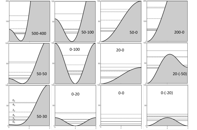
Figure 1: Energies of the low-lying states of the phenomenological Gamma-rotor Hamiltonian (3) caprio11 for characteristic potentials, which are labeled by their parameters $\chi-\kappa$. The abscissas represent the triaxiality parameter $0\leq\gamma\leq\pi/3$. The ordinates represent the energies of the displayed quantities in units of $\hbar^{2}/B\beta^{2}$, where the range is [0,100], except for the potentials 500-400 and 200-0, where the range is [0,200]. The horizontal lines show the energies of the heads of the low-lying bands, which are labeled by their $I^{+}_{n}$ in the spectrum for the potential 50-30. Rescaling the energies by the factor $E(2^{+}_{1})_{exp}/E(2^{+}_{1})_{GR}$ adapts the potentials to the experimental energy scale, where $E(2^{+}_{1})_{GR}$ is given in Table 1.

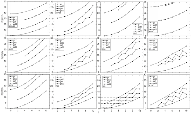
Figure 2: Rotational sequences on the low-lying states of the potentials shown in Fig. 1. (Note the different scales of 500-400, 200-0 and 20-(-50)). The dashed lines for the $\gamma$-independent potential 0-0 connect the states of the seniority $v$, which is equal to $I/2$ of the yrast states. The labelling of the bands in the legend is as follows, gr : ground/yrast-band, ga1 : $\gamma$-band, ga22 : $\gamma\gamma$4-band and ga20 : $\gamma\gamma$0-band.

Table 1: Energy characteristics of the potentials plotted in Fig. 1 . The staggering parameter $\bar{S}(I)$ is defined by Eq. (6). The excitation energy $E(2^{+}_{1})_{GR}$ is the difference $E(2^{+}_{1})-E(0^{+}_{1})$ of the eigenvalues of the Gamma-rotor Hamiltonian (3).

$\chi-\kappa$	$E(2^{+}_{1})_{GR}$	$\gamma_{m}$	$\Delta\gamma$	${\left[\frac{E(2^{+}_{2})}{E(2^{+}_{1})}\right]}$	${\left[\frac{E(2^{+}_{2})}{E(4^{+}_{1})}\right]}$	$\bar{S}(6)$
200-0	2.15	0	14	26.8	8.07	-0.03
100-0	2.24	0	17	18.0	3.31	-0.14
50-0	2.39	0	20	11.6	3.55	-0.51
20-0	2.87	0	24	5.82	1.93	-1.75
10-0	3.42	0	27	3.61	1.32	-2.49
0-0	4.00	30	60	2.50	1.00	-2.75
0-200	3.05	30	16	2.11	0.81	3.87
0-100	3.57	30	19	2.21	0.86	3.12
0-50	3.80	30	21	2.34	0.92	1.61
0-20	3.95	30	22	2.45	0.98	0.50
50-100	3.10	25	19	3.50	1.20	1.85
500-400	2.34	17	15	10.8	3.17	0.32
50-50	2.73	20	26	6.01	1.92	0.30
50-30	2.58	11	26	7.78	2.44	-0.35
0- -20	3.39	30	35	2.42	0.96	-5.79
20- -50	2.35	34	17	11.74	3.62	-5.55

Table 2: Transition probabilities that characterize the potentials in Fig. 1 in units of $B(E2,2^{+}_{1}\rightarrow 0^{+}_{1})$. The $B(E2,4^{+}_{3}\rightarrow 2^{+}_{1})$ values are smaller than 0.003.

$\chi-\kappa$	$Q(2^{+}_{1})$	$Q(2^{+}_{2})$	$B(E2,2^{+}_{2}\rightarrow 0^{+}_{1})$	$B(E2,4^{+}_{3}\rightarrow 2^{+}_{2})$	$B(E2,2^{+}_{2}\rightarrow 2^{+}_{1})$	$B(E2,0^{+}_{2}\rightarrow 2^{+}_{2})$	$B(E2,0^{+}_{2}\rightarrow 2^{+}_{1})$	$B(E2,2^{+}_{3}\rightarrow 0^{+}_{1})$	$B(E2,3^{+}_{1}\rightarrow 2^{+}_{1})$	$B(E2,3^{+}_{1}\rightarrow 2^{+}_{2})$
200-0	-0.888	0.873	0.033	0.094	0.056	0.195	0.001	0.002	0.059	1.715
100-0	-0.878	0.859	0.047	0.130	0.086	0.304	0.004	0.003	0.084	1.675
50-0	-0.861	0.840	0.064	0.164	0.143	0.527	0.009	0.008	0.114	1.595
20-0	-0.797	0.789	0.079	0.106	0.347	1.193	0.030	0.004	0.136	1.362
10-0	-0.656	0.655	0.060	0.030	0.719	1.550	0.040	0.003	0.097	1.235
0-0	0.000	0.000	0.000	0.000	1.428	1.666	0.000	0.000	0.000	1.190
0-200	0.000	0.000	0.000	0.000	1.422	0.102	0.000	0.000	0.000	1.763
0-100	0.000	0.000	0.000	0.000	1.416	0.208	0.000	0.000	0.000	1.723
0-50	0.000	0.000	0.000	0.000	1.413	0.445	0.000	0.000	0.000	1.663
0-20	0.000	0.000	0.000	0.000	1.421	0.922	0.000	0.000	0.000	1.458
50-100	-0.693	0.684	0.084	0.180	0.629	0.247	0.011	0.001	0.148	1.704
500-400	-0.861	0.851	0.066	0.130	0.143	0.142	0.004	0.003	0.118	1.736
50-50	-0.807	0.789	0.091	0.186	0.316	0.425	0.016	0.002	0.160	1.634
50-30	-0.835	0.815	0.082	0.181	0.227	0.492	0.014	0.002	0.144	1.609
0- -20	0.000	0.000	0.000	0.000	1.411	2.810	0.000	0.000	0.000	0.785
20- -50	-0.868	0.874	0.032	0.016	0.089	2.995	0.009	0.022	0.0921	0.750

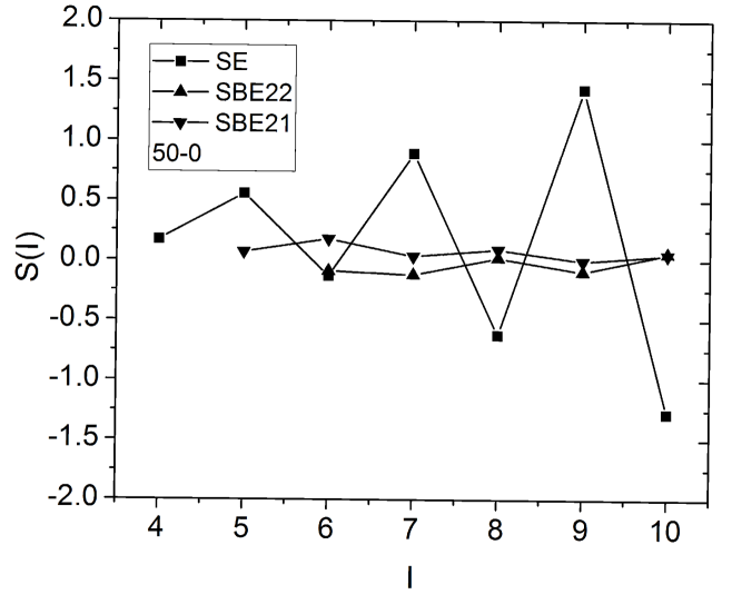
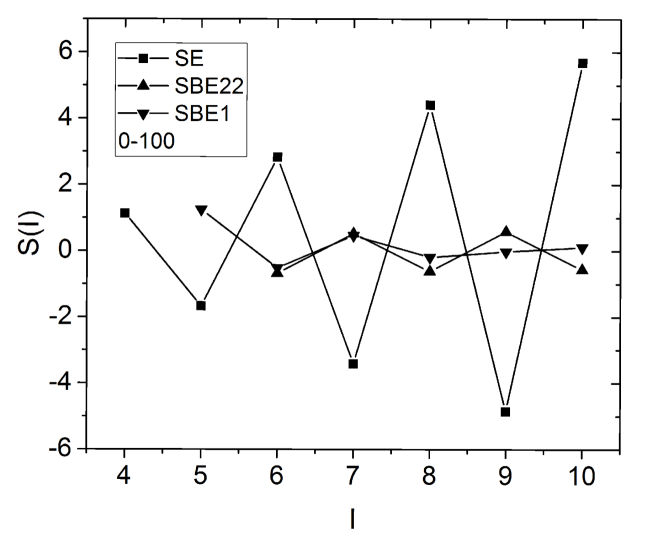
Figure 3: Staggering parameter $S(I)$ calculated by Eq. (1) from the energies ($SE$) and by the analog equations (7) from the $B(E2,I\rightarrow I-2)$ values ($SBE22$) and (8) from the $B(E2,I\rightarrow I-1)$ values ($SBE21$). The upper panel shows the soft prolate potential 50-0 and the lower panel triaxial potential 0-100.

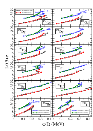
Figure 4: (Color online) Angular momentum as function of the angular frequency for the yrast and the $\gamma$-bands after configuration mixing compared with experimental data for the ^154,156Gd, ^{156,158,160,162}Dy, ^164,166,170Er, ¹⁸⁰Hf, ²³²Th and ²³⁸U isotopes. A shift $c=10$ is added for the $\gamma$-bands. The even-I states $(\alpha=0)$ are shown as circles and the odd-I $(\alpha=1)$ states as squares. (Data taken from NNDC ; Lee1980 ; Emling1981 ; Majola2015 ).

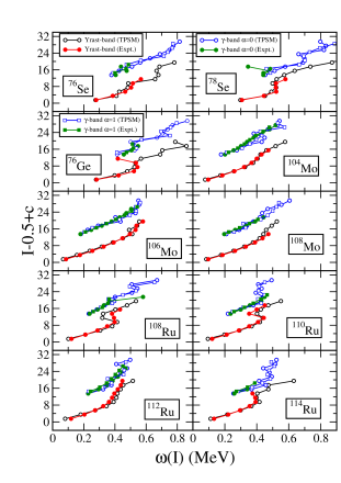
Figure 5: (Color online) Angular momentum as function of the angular frequency for the yrast and the $\gamma$-bands after configuration mixing compared with experimental data for the ^76,78Se, ⁷⁶Ge, ^104,106,108Mo and ^{108,110,112,114}Ru isotopes. A shift $c=10$ is added for the $\gamma$-bands. The even-I states $(\alpha=0)$ are shown as circles and the odd-I $(\alpha=1)$ states as squares. (Data taken from NNDC ; Musangu2021 ).

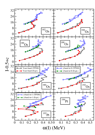
Figure 6: (Color online) Angular momentum as function of the angular frequency for the yrast and the $\gamma$-bands after configuration mixing compared with experimental data for the ^182-192Os and ^192,194Pt isotopes. A shift $c=10$ is added for the $\gamma$-bands. (Data taken from NNDC ).

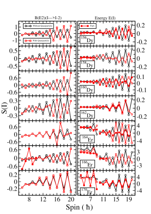
Figure 7: (Color online) Staggering parameters $S(I)$ calculated by means of Eq. (1) from the energies of the $\gamma$-band (right panels) and by the analogue equation (7) from the intra $\gamma$-band $B(E2,I\rightarrow I-2)$ values (left panels). For the Er isotopes, $10\times S(I)$ is displayed for $I\leq 9$ in order to resolve the details of the small staggering.

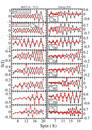
Figure 8: (Color online) Staggering parameters $S(I)$ calculated by means of Eq. (1) from the energies of the $\gamma$-band (right panels) and by the analogue equation (7) from the intra $\gamma$-band $B(E2,I\rightarrow I-2)$ values (left panels).

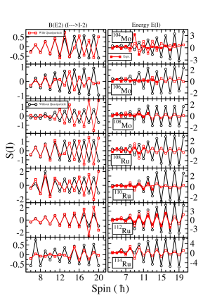
Figure 9: (Color online) Staggering parameters $S(I)$ calculated by means of Eq. (1) from the energies of the $\gamma$-band (right panels) and by the analogue equation (7) from the intra $\gamma$-band $B(E2,I\rightarrow I-2)$ values (left panels).

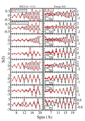
Figure 10: (Color online) Staggering parameters $S(I)$ calculated by means of Eq. (1) from the energies of the $\gamma$-band (right panels) and by the analogue equation (7) from the intra $\gamma$-band $B(E2,I\rightarrow I-2)$ values (left panels).

2 Triaxiality and $\gamma$-softness

The concepts of triaxiality and $\gamma$-softness have been developed in the context of the phenomenological Bohr Hamiltonian, see Refs. BM75 , p. 677 ff. and RW10 , p. 97 ff. In order to quantify them in terms of the low-energy observables, we assume that the deformation parameter $\beta$ is fixed, i.e., only the triaxiality parameter $\gamma$ and the orientation angles are considered as dynamical variables. The model is presented as "Gamma-rotor" in Ref. caprio11 . The nature of the triaxiality can be characterized by the $\gamma$-dependence of the potential.

The shape of the nuclear surface is defined by the quadrupole deformation parameters

$$\alpha_{\mu}=\beta\left[\cos\gamma\,{\cal D}^{(2)}_{0\mu}(\Omega)+\frac{1}{\sqrt{2}}\sin\gamma\left[{\cal D}^{(2)}_{2\mu}(\Omega)+{\cal D}^{(2)}_{-2\mu}(\Omega)\right]\right],$$ (2)

where $\beta$ is the deformation parameter, $\gamma$ the triaxiality parameter and $\Omega$ are the Euler angles, specifying the orientation of the shape. The Hamiltonian in units of $\hbar^{2}/B\beta^{2}$ is given by

$$H_{GR} = \hat{\Lambda}^{2}+V(\gamma)_{GR}$$ (3)

$$= \hat{\Lambda}^{2}+\chi(1-\cos 3\gamma)+\kappa(\cos^{2}3\gamma-1),$$

where $B$ sets the scale of the kinetic energy, and

$$\hat{\Lambda}^{2}=-\biggl{(}\frac{1}{\sin 3\gamma}\frac{\partial}{\partial\gamma}\sin 3\gamma\frac{\partial}{\partial\gamma}-\frac{1}{4}\sum_{i=1,2,3}\frac{\hat{L}_{i}^{\prime 2}}{\sin^{2}(\gamma-\frac{2}{3}\pi i)}.\biggr{)}.$$ (4)

with “$\hat{L}_{i}^{\prime}$” being the angular momentum components with respect to the body-fixed axes. The kinetic energy operator, $\hat{\Lambda}^{2}$, is the Laplacian in five dimensions. It is the Casimir operator for the five-dimensional rotation group SO(5), which contains the rotations in physical space, acting on the Euler angle coordinates as an SO(3) subgroup. The potential energy $V(\beta,\gamma)$ must be periodic in $\gamma$ with period of $120^{\circ}$, and it must be symmetric about $\gamma=0^{\circ}$ and $\gamma=60^{\circ}$.

The matrix elements of the charge quadrupole moments, which generate the $B(E2)$ $\gamma$-transitions and the static electric quadrupole matrix elements, are modeled by a homogeneous charged droplet

$$Q_{\mu}=\frac{3ZR_{0}^{2}}{4\pi}\left(e\alpha_{\mu}^{*}-\frac{10}{\sqrt{70\pi}}e^{2}[\alpha\times\alpha]^{(2)*}_{\mu}\right),$$ (5)

where “$e$” fixes the scale.

Fig. 1 illustrates a selection of potential types, and Fig. 2 shows the low-lying bands that belong to these potentials. Tables 1 and 2 list quantities that characterize the collective mode. The results for several potentials, not shown in Fig. 1, are added to better display their parameter dependence. In Table 1, the position of the minimum (maximum) of the potentials is listed as $\gamma_{m}$. The softness of the potentials $\Delta\gamma$ is quantified as the distance between zero and the turning point or the two turning points of the classical motion for the Gamma-rotor Hamiltonian (3) with the angular momentum $L=0$ and energy $E$ equal to the quantal energy of the $0^{+}_{1}$ state, which is the length of the corresponding bars in Fig. 1. It is a measure of the ground-state fluctuation in $\gamma$, which coincides with the oscillator length in the case of the harmonic limit. The next columns list important energy criteria characterizing the nature of triaxiality, namely the ratios ${\left[\frac{E(2^{+}_{2})}{E(2^{+}_{1})}\right]}$, ${\left[\frac{E(2^{+}_{2})}{E(4^{+}_{1})}\right]}$ and the modified staggering parameter $\bar{S}(6)$ , which is defined as

$$\bar{S}(I)=\frac{S(I)-S(I+1)}{2}.$$ (6)

The latter is more appropriate in tables that cite only the value for one $I$, because it oscillates around zero, while $S(I)$ oscillates around some positive value which represents the curvature of the rotational energy.

The lowest rotational sequences in Fig. 2 have the following general characteristics. Consider the potential $\chi-\kappa=200-0$, which represents a rigid prolate nucleus with harmonic $\gamma$-vibrational excitations. The $\Delta I=2$ ground-band on the $0^{+}_{1}$ state represents the zero-phonon sequence. The one-phonon single $\gamma$-band ($\gamma$) is the $\Delta I=1$ rotational sequence on the $2^{+}_{2}$ state. It represents a traveling wave, which classically corresponds to a triaxial distortion that rotates around the symmetry axis. The two-phonon double $\gamma$-band ($\gamma\gamma 4$) is the $\Delta I=1$ rotational sequence on the $4^{+}_{3}$ state. It represents a traveling wave generated by adding a second $K=2$ on top of the first with the same angular momentum along the symmetry axis. The second two-phonon double $\gamma$-band ($\gamma\gamma 0$) is the $\Delta I=2$ rotational sequence on the $0^{+}_{2}$ state. It is generated by putting the second phonon with opposite angular momentum projection on the symmetry axis on top of the first. It represents a pulsating wave, which classically corresponds to an oscillation of the triaxial deformation between the prolate and oblate turning points. (For a discussion of the classical correspondence see also Ref. BM75 p. 656.)

The lowest bands keep their character when the potential deviate from the harmonic limit. Making the axial potential more shallow by reducing the strength of the $\chi(1-\cos 3\gamma)$ term (see 50-0 and 20-0)) brings down the $\gamma$-excitations and generates couplings between them, which shift the energies. As discussed in detail in the Appendix, the repulsion between the even-$I$ states of the $\gamma\gamma 0$ and the $\gamma$-bands prevail, which results in the even-$I$-down staggering pattern that signifies $\gamma$-softness. Adding the $\xi(\cos^{2}3\gamma-1)$ term shifts the $\gamma$-band towards the ground-band (see the potentials 50-50 and 50-100 in Table 1). The repulsion between the even-$I$ states of the ground-band and the $\gamma$-band generates the even-$I$-up staggering pattern that characterizes $\gamma$-rigidity. The competition between the two effects is reflected by the transition from a soft axial to a soft triaxial potential. As seen in Fig. 2 and Table 1, the down-shift by the $\gamma\gamma 0$-band prevails for the 50-0 potential, the up-shift by the ground-band prevails for the 0-50 potential, and both shifts largely compensate each other for the potential 50-50.

In the Appendix we discuss in detail how characteristic relations between energies and $E2$ transition rates between the states in the yrast region emerge for the various the potentials, and how they can be understood in terms of the couplings between the lowest bands. Such an interpretation is useful because it applies in an analogous way to the TPSM results discussed later. Further details can be found in Ref. caprio11 .

Fig. 3 shows the staggering parameters $S(I)$ calculated by means of Eq. (1) from the energies of the $\gamma$-bands of the soft prolate potential 50-0 and the triaxial potential 0-100. Added are plots of the staggering of the intra-band $B(E2,I\rightarrow I-2)$ values ($SBE22$) and of intraband the $B(E2,I\rightarrow I-1)$ values ($SBE21$)

$$SBE22(I)=[B(E2,I_{\gamma}\rightarrow I_{\gamma}-2)$$

$$-2(B(E2,I_{\gamma}-1\rightarrow I_{\gamma}-3)$$

$$+(B(E2,I_{\gamma}-2\rightarrow I_{\gamma}-4)]/B(E2,2^{+}_{1}\rightarrow 0^{+}_{1}),$$ (7)

$$SBE21(I)=[B(E2,I_{\gamma}\rightarrow I_{\gamma}-1)$$

$$-2(B(E2,I_{\gamma}-1\rightarrow I_{\gamma}-2)$$

$$+(B(E2,I_{\gamma}-2\rightarrow I_{\gamma}-3)]/B(E2,2^{+}_{1}\rightarrow 0^{+}_{1}).$$ (8)

As seen the transition probabitlies show a weak staggering with the opposite phase as that of the energies. As discussed above, the staggering of the energies can be explained by the mixing of the even-$I$-states of $\gamma$-band with the states of the ground- and $\gamma\gamma 0$-bands. The staggering of the $B(E2)$ values can be explained in the same way, in particular its opposite phase. The explanation is somewhat complex as it involves the phases of the mixed states and is given in the Appendix.

The SO(5) Laplacian (4) is invariant under the transformation $\gamma\rightarrow 60^{\circ}-\gamma$ and an exchange of the three principal axes, which leads to a symmetry quantum number called $\gamma$-parity RW10 . The potential term “$\cos 3\gamma$” is odd under this transformation and it has no diagonal matrix elements in the absence of a potential. As a consequence, changing from prolate to oblate shape by $\chi\rightarrow-\chi$, will give the same energies. Moreover, the $E2$ transition operator transforms in a simple way (see RW10 p. 222 ff. ) such that all $B(E2,I\rightarrow I^{\prime})$ values are the same as well, while the static quadrupole moment change their signs. For this reason only the potentials with prolate preference are discussed. The cases with oblate preference are given by this symmetry. The sign change of the quadrupole operator implies that for the potentials that are symmetric about $\gamma=30^{\circ}$ the static quadrupole moments $Q(2^{+}_{2})=-Q(2^{+}_{1})=0$ as well as $B(E2,4^{+}_{2}\rightarrow 2^{+}_{2})=B(E2,2^{+}_{2}\rightarrow 0^{+}_{1})=0$.

The following classification scheme seems appropriate. The potential is called "prolate" if $\gamma_{m}=0^{\circ}$, "triaxial" if $\gamma_{m}>0^{\circ}$ and "transitional" if its curvature at $\gamma=0^{\circ}$ is close to zero (50-30 in Fig. 1). For $\Delta\gamma\leq 16^{\circ}$, we further specify. the potential as "rigid", for $16^{\circ}\leq\Delta\gamma\leq 25^{\circ}$ as "soft", and for $\Delta\gamma\geq 25^{\circ}$ as "shallow". Of course, the boundaries are not sharp and to some extent arbitrarily chosen. The potentials determine the density distributions. Thus it appears appropriate to classify, loosely speaking, the "nuclear shapes" in the same way.

The signatures of triaxility and $\gamma$-softness from the perspective of a collective model can be summarized as follows:

1) The deviation from axial shape is indicated by the energy of the $2^{+}_{2}$ state ($\gamma$-band head) relative to the $4^{+}_{1}$ level of the ground-band. This relative differences changes from a larger value for narrow axial potential to $E(2^{+}_{2})=E(4^{+}_{1})$ for the $\gamma$-independent potential to $E(2^{+}_{2})<E(4^{+}_{1})$ for a stiff triaxial potential.
2) The staggering parameter $S(I)$ is a measure for the $\gamma$-softness. A large even-$I$-down amplitude indicates a shallow potential. A small even-$I$-down amplitude and $E(2^{+}_{2})>>E(4^{+}_{1})$ indicate a narrow axial potential. A large odd-$I$-down amplitude indicates a narrow triaxial potential. A small amplitude of $S(I)$ and $E(2^{+}_{2})$ near $E(4^{+}_{1})$ indicate a soft potential transitional between axial and triaxial.
3) The symmetry of the potential with respect to $\gamma=30^{\circ}$ is reflected by the static quadrupole moments $Q$ of the $2^{+}$ states. For a potential preferring $\gamma<30^{\circ}$ one has $Q(2^{+}_{1}$)<0 and $Q(2^{+}_{2})=-Q(2^{+}_{1})$. For a potential preferring $\gamma>30^{\circ}$ one has $Q(2^{+}_{1}$>0 and $Q(2^{+}_{2})=-Q(2^{+}_{1})$. For a symmetric potential $Q(2^{+}_{2})=-Q(2^{+}_{1})$=0 and $B(E2,2^{+}_{1}\rightarrow 0^{+}_{1})$=0, and $B(E2,2^{+}_{2}\rightarrow 2^{+}_{1})$ is large. Deviations from symmetry quickly remove the quenching and reduce the $B(E2,2^{+}_{2}\rightarrow 2^{+}_{1})$ value.
4) For all potentials, the band built on the $0^{+}_{2}$ represents an oscillation of $\gamma$ around the potential minimum at $\gamma_{m}$ with two-phonon nature $\gamma\gamma 0$. The transition probability $B(E2,0^{+}_{2}\rightarrow 2^{+}_{2})$ to the one-phonon state is large when the pattern of staggering parameter $S(I)$ is strongly even-$I$-down.

3 Triaxial projected shell model calculations

The TPSM approach employs the methodology similar to that of the standard spherical shell model, except that deformed angular momentum projected basis are used to diagonalize the shell model Hamiltonian JS16 ; Hara1995 . The Hamiltonian in the TPSM approach contains the standard pairing plus quadrupole-quadrupole interaction terms, and is given by

$$\hat{H}=\hat{H}_{0}-{\chi\over 2}\sum_{\mu}\hat{Q}^{\dagger}_{\mu}\hat{Q}_{\mu}-G_{M}\hat{P}^{\dagger}\hat{P}-G_{Q}\sum_{\mu}\hat{P}^{\dagger}_{\mu}\hat{P}_{\mu}.$$ (9)

The terms in the above equation (9) represent the modified harmonic oscillator single-particle Hamiltonian Ni69 , monopole pairing, quadrupole pairing, and quadrupole-quadrupole interaction, respectively. The value of $\chi$, the $QQ$-force strength, is fixed such that the quadrupole mean-field is obtained through Hartree-Fock-Bogoliubov self-consistency condition Hara1995 :

$$\chi_{\tau\tau^{\prime}}={{2\over 3}\epsilon\hbar\omega_{\tau}\hbar\omega_{\tau^{\prime}}\over\hbar\omega_{n}\langle\hat{Q}_{0}\rangle_{n}+\hbar\omega_{p}\langle\hat{Q}_{0}\rangle_{p}}$$ (10)

where $\omega_{\tau}=\omega_{0}a_{\tau}$, with $\hbar\omega_{0}=41.4678A^{-{1\over 3}}$MeV, and

$$a_{\tau}=\left[1\pm{{N-Z}\over A}\right]^{{1\over 3}}$$ (11)

controls isospin-dependence with $+(-)$ for neutrons (protons).

For the monopole pairing strength, the coupling constant $G_{M}$ is of the standard form

$$G_{M}=\left(G_{1}\mp G_{2}{{N-Z}\over A}\right){1\over A}$$ (12)

with $-(+)$ referring to neutrons (protons). The values of $G_{1}$ and $G_{2}$ for a particular mass region are adjusted in such a way that the calculated gap parameters reproduce the experimental odd-even mass differences. The coupling constant $G_{Q}$ of quadrupole pairing is $0.18G_{M}$. The pairing parameters are taken from our previous work SJ21 and are listed in Table 1 of this reference.

The deformed shell model basis is constructed from BCS quasiparticle configurations generated from the eigenstates of the triaxial Nilsson potential with the axial deformation parameter $\varepsilon$ and the non-axial parameter $\varepsilon^{\prime}$ and the BCS gaps determined by the selfconsistency conditions $\Delta_{M}=G_{M}\langle P\rangle$ and $\Delta_{\mu}=G_{Q}\langle P_{\mu}\rangle$. The quasiparticle configurations are projected onto good angular momentum states using the three-dimensional projection operator RS80 . The diagonalization of the shell model Hamiltonian (9) is then performed using the angular momentum projected multi-quasiparticle basis states. The multi-quasiparticle basis space used in the present work are given by $:$

$$\hat{P}^{I}_{MK}\,|\,\Phi\rangle;$$

$$\hat{P}^{I}_{MK}~{}a^{\dagger}_{p_{1}}a^{\dagger}_{p_{2}}\,|\,\Phi\rangle;$$

$$\hat{P}^{I}_{MK}~{}a^{\dagger}_{n_{1}}a^{\dagger}_{n_{2}}\,|\,\Phi\rangle;$$ (13)

$$\hat{P}^{I}_{MK}~{}a^{\dagger}_{p_{1}}a^{\dagger}_{p_{2}}a^{\dagger}_{n_{1}}a^{\dagger}_{n_{2}}\,|\,\Phi\rangle,$$

where the subscript $n$ denotes the quasineutron and $p$ the quasiproton states, $\,|\,\Phi\rangle$ represents the triaxially-deformed quasiparticle vacuum state, and $P^{I}_{MK}$ is the three-dimensional angular momentum projection operator in its standard form RS80 ; HS79 ; HS80

$$\hat{P}^{I}_{MK}={2I+1\over 8\pi^{2}}\int~{}d\Omega\,D^{I}_{MK}(\Omega)\,\hat{R}(\Omega).$$ (14)

Here

$$\hat{R}(\Omega)=e^{-i\alpha\hat{J}_{z}}e^{-i\beta\hat{J}_{y}}e^{-i\gamma\hat{J}_{z}}~{}~{}~{}.$$ (15)

is the rotation operator, $D^{I}_{MK}(\Omega)$ is the Wigner $D$-function BM75 , $\Omega$ represents the set of Euler angles ($\alpha,\gamma=[0,2\pi],\,\beta=[0,\pi]$), and $\hat{J}_{x,y,z}$ are the angular momentum operators.

The Hamiltonian in Eq. (9) is diagonalized using the non-orthogonal basis of Eq. (3), which leads to the generalized eigenvalue problem

$$\sum_{K^{\prime},\kappa^{\prime}}(\,<\!\Phi_{\kappa}| \hat{H} \hat{P}^{I}_{KK^{\prime}}|\Phi_{\kappa^{\prime}}\!>\,$$

$$- E_{l\sigma}\,<\!\Phi_{\kappa}|\hat{P}^{I}_{KK^{\prime}}|\Phi_{\kappa^{\prime}}\!>\,)f^{\sigma I}_{K^{\prime}\kappa^{\prime}}=0$$

with the projected wavefunction

$$\,|\,\psi^{\sigma I}\rangle=\sum_{K,\kappa}~{}f^{\sigma I}_{K\kappa}~{}\hat{P}^{I}_{MK}|~{}\Phi_{\kappa}\!>\,.$$ (17)

The symbol $\kappa$ represents quasiparticle configurations of the basis states Eq. (3). A new set of components is introduced WANG2020

$$g^{\sigma I}_{K\kappa}=\sum_{K^{\prime},\kappa^{\prime}}\,<\!\Phi_{\kappa}|\hat{P}^{I}_{KK^{\prime}}|\Phi_{\kappa^{\prime}}\!>\,^{1/2}f^{\sigma I}_{K^{\prime}\kappa^{\prime}},$$ (18)

which are orthonormal, and $|g^{I}_{K,\kappa}|^{2}$ is the probability of a projected quasiparticle configuration in the wave function (17).

The electromagnetic transition probabilities are obtained using the expression $:$

$$B(E2,I_{i}\rightarrow I_{f})={e^{2}\over{2I_{i}+1}}\,|\,\langle\psi^{\sigma_{f}I_{f}}\,|\,\,|\,\hat{Q}_{2}\,|\,\,|\,\psi^{\sigma_{i}I_{i}}\rangle\,|\,^{2}$$ (19)

from an initial state $\psi^{\sigma_{i}I_{i}}$ to a final state $\psi^{\sigma_{f}I_{f}}$. Effective charges of 1.5e (0.5e) for protons (neutrons) similar to our previous publications GH14 ; bh15 ; SJ18 are used in our calculations.

For an irreducible spherical tensor, $\hat{Q}$, of rank $L$, the reduced matrix element can be expressed as

$$\langle\psi^{\sigma_{f}I_{f}}\,|\,\,|\,\hat{Q}_{L}\,|\,\,|\,\psi^{\sigma_{i}I_{i}}\rangle$$

$$~{}~{}~{}~{}~{}~{}~{}~{}=\sum_{\kappa_{i},\kappa_{f},K_{i},K_{f}}f_{\kappa_{i}K_{i}}^{\sigma_{i}I_{i}}f_{\kappa_{f}K_{f}}^{\sigma_{f}I_{f}}\sum_{M_{i},M_{f},M}(-)^{I_{f}-M_{f}}$$

$$~{}~{}~{}~{}~{}~{}~{}~{}~{}~{}~{}~{}~{}~{}~{}~{}~{}~{}~{}~{}~{}~{}~{}~{}\times\begin{pmatrix}I_{f}&L&I_{i}\\ -M_{f}&M&M_{i}\end{pmatrix}$$

$$~{}~{}~{}~{}~{}~{}~{}~{}~{}~{}~{}~{}~{}~{}~{}~{}\times\langle\Phi_{\kappa_{f}}\,|\,\hat{P}_{K_{f}M_{f}}^{I_{f}}\hat{Q}_{LM}\hat{P}_{K_{i}M_{i}}^{I_{i}}\,|\,\Phi_{\kappa_{i}}\rangle$$ (20)

$$~{}~{}~{}~{}~{}~{}~{}~{}=2\sum_{\kappa_{i},\kappa_{f},K_{i},K_{f}}f_{\kappa_{i}K_{i}}^{\sigma_{i}I_{i}}f_{\kappa_{f}K_{f}}^{\sigma_{f}I_{f}}\sum_{M^{\prime},M^{\prime\prime}}(-)^{I_{f}-K_{f}}(2I_{f}+1)^{-1}$$

$$~{}~{}~{}~{}~{}~{}~{}~{}~{}~{}~{}~{}~{}~{}~{}~{}\times\begin{pmatrix}I_{f}&L&I_{i}\\ -K_{f}&M^{\prime}&M^{\prime\prime}\end{pmatrix}\int d\Omega D_{M^{\prime\prime}K_{i}}^{I_{i}}(\Omega)$$

$$~{}~{}~{}~{}~{}~{}~{}~{}~{}~{}~{}~{}~{}~{}~{}~{}~{}~{}~{}~{}~{}~{}~{}~{}\times\langle\Phi_{\kappa_{f}}\,|\,\hat{Q}_{LM^{\prime}}\hat{R}(\Omega)\,|\,\Phi_{\kappa_{i}}\rangle.$$

The symbol ( ) in the above expression represents $3j$-coefficient.

It is important to point out that the triaxiality parameter $\gamma_{N}=\arctan(\varepsilon^{\prime}/\varepsilon)$ merely controls the Nilsson Hamiltonian, which generates the deformed single particle orbits. The "geometric" triaxiality parameter $\gamma$ of the nuclear charge and mass distributions calculated from the TPSM wavefunctions differs from $\gamma_{N}$. The authors of Ref. Shimizu08 gave an approximate estimate based on the volume conserving deformed oscillator, which is the basis of the Nilsson Hamiltonian,

$$\omega_{i}=\omega_{0}\left[1-\frac{2}{3}\varepsilon\cos\left(\gamma_{N}+i\frac{2\pi}{3}\right)\right],$$ (21)

$$\tan(\gamma)=\frac{\sqrt{3}(\omega_{2}^{-2}-\omega_{1}^{-2})}{2\omega_{3}^{-2}-\omega_{1}^{-2}-\omega_{2}^{-2}},~{}~{}~{}\gamma\approx\left(1-\frac{3}{2}\varepsilon\right)\gamma_{N},$$ (22)

where the approximation hold for small $\gamma$. The triaxiality parameter $\gamma$, which concerns the collective Bohr Hamiltonian, is substantially smaller than $\gamma_{N}$. For example, the TPSM parameters for ¹⁶⁶Er are $\varepsilon$=0.325, $\varepsilon^{\prime}$=0.120, that is $\gamma_{N}=21^{\circ}$, which corresponds to $\gamma=13^{\circ}$.

The detailed results of energies and quadrupole transitions of thirty nuclei studied in the present work are presented in Figs. 4 - 28 and Tables 3 - 6.

Table 3: Axial and triaxial quadrupole deformation parameters $\epsilon$ and $\epsilon^{\prime}$ employed in the TPSM calculation. Axial deformations are taken from our earlier works GH14 ; GH08 ; bh15 ; GS12 ; SJ21 and raman , and nonaxial deformations are chosen in such a way that heads of the $\gamma$-bands are reproduced. In this table, we also provide the energy $E(2^{+}_{1})$, the ratios, ${\frac{E(2^{+}_{2})}{E(2^{+}_{1})}}$ and ${\frac{E(2^{+}_{2})}{E(4^{+}_{1})}}$, $\bar{S}(I=6)=\frac{S(I=6)-S(I=7)}{2}$ and also $B(E2,2_{1}^{+}\rightarrow 0_{1}^{+})$ and $B(E2,2_{2}^{+}\rightarrow 0_{1}^{+})$ (in W.u.) with both experimental (error bars in curly brackets, data taken from raman ; Singh1984 ; Farhan2009 ; Blach2007 ; Fren2008 ; Blach2000 ; Gurdal2012 ; Lalkov2015 ; Reich2009 ; Reich2012 ; Nica2017 ; Nica2021 ; Reich2007 ; Singh2018 ; Baglin2008 ; Baglin2018 ; Wu2003 ; Singh2015 ; Baglin2010 ; Baglin2003 ; Singh2002 ; Singh190 ; Baglin2012 ; Chen194 ; Browne2006 ; Martin2002 ) and TPSM predicted values.

Isotope	$\epsilon$	$\epsilon^{\prime}$	$\gamma_{N}$	$E(2_{1}^{+})$	${\left[\frac{E(2^{+}_{2})}{E(2^{+}_{1})}\right]}$	${\left[\frac{E(2^{+}_{2})}{E(4^{+}_{1})}\right]}$	$\bar{S}(I=6)$	$B(E2)(2_{1}^{+}\rightarrow 0_{1}^{+})$	$B(E2)(2_{2}^{+}\rightarrow 0_{1}^{+})$
					TPSM (Expt.)	TPSM (Expt.)	TPSM (Expt.)	TPSM (Expt.)	TPSM (Expt.)
76Ge	0.200	0.160	38.6	0.558 (0.563)	2.1 (1.9)	0.89 (0.78)	0.194 (0.124)	22.42 (29 {1})	4.08 (0.9 {22})
76Se	0.260	0.155	30.8	0.551 (0.559)	2.2 (2.2)	0.89 (0.91)	-0.107 (0.487)	46.08 (44 {1})	0.98 (1.3 {1})
78Se	0.256	0.150	30.2	0.595 (0.613)	2.2 (2.1)	0.87 (0.87)	-0.384 (-0.242)	34.65 (33.5 {8})	1.85 (0.76 {6})
104Mo	0.320	0.130	22.1	0.154 (0.192)	5.3 (4.2)	1.64 (1.45)	-0.328 (-0.184)	93.61 (92 {6})	19.14
106Mo	0.310	0.110	19.5	0.135 (0.171)	5.1 (4.1)	1.55 (1.36)	-0.285 (-0.091)	89.79 (102.3 {25})	15.94
108Mo	0.294	0.140	25.4	0.168 (0.193)	3.6 (3.0)	1.16 (1.04)	-0.306 (-0.031)	102.48 (104.74 {10})	16.5
108Ru	0.280	0.150	28.2	0.202 (0.242)	3.5 (2.9)	1.14 (1.07)	-0.065 (-0.322)	61.12 (58.0 {5})	21.62
110Ru	0.290	0.150	27.3	0.188 (0.240)	3.4 (2.5)	1.10 (0.92)	0.189 (-0.011)	68.11 (66.0 {5})	17.64
112Ru	0.289	0.130	24.2	0.161 (0.236)	3.2 (2.2)	0.98 (0.81)	0.854 (0.314)	69.73 (70.0 {7})	11.89
114Ru	0.250	0.080	17.7	0.222 (0.265)	2.4 (2.1)	0.82 (0.79)	0.909 (0.357)	66.73	7.01
154Gd	0.300	0.100	18.4	0.095 (0.123)	10.6 (8.1)	3.18 (2.68)	-0.013 (-0.013)	165.77 (157.0 {1})	8.4 (5.7 {5})
156Gd	0.341	0.100	16.3	0.092 (0.089)	12.1 (12.9)	3.66 (4.00)	-0.023 (-0.04)	186.48 (189.0 {3})	9.29 (4.68 {16})
156Dy	0.278	0.105	20.7	0.093 (0.138)	10.05 (6.5)	3.06 (2.20)	0.003 (0.004)	161.93 (150.0 {17})	9.51
158Dy	0.260	0.110	22.9	0.079 (0.098)	12.01 (9.6)	3.63 (2.98)	-0.012 (0.007)	190.66 (186.0 {4})	7.58
160Dy	0.270	0.110	22.1	0.074 (0.087)	12.9 (11.1)	3.92 (3.40)	0.003 (-0.008)	181.55 (195.8 {25})	7.34 (4.46 {+33-29})
162Dy	0.280	0.120	23.2	0.077 (0.081)	11.0 (10.9)	3.33 (3.34)	-0.004 (-0.004)	201.76 (204.0 {3})	7.64 (4.6 {3})
164Er	0.317	0.120	20.7	0.087 (0.091)	9.9 (9.4)	3.01 (2.87)	-0.029 (-0.019)	208.03 (206 {5})	9.51 (5.3 {6})
166Er	0.325	0.126	21.2	0.066 (0.081)	11.1 (9.7)	3.35 (2.96)	0.055 (0.007)	228.13 (217.0 {5})	6.79 (5.17 {21})
170Er	0.319	0.110	19.0	0.069 (0.078)	14.3 (11.8)	4.31 (3.59)	0.074 (0.386)	215.96 (208.0 {4})	8.03 (3.68 {11})
180Hf	0.195	0.090	24.7	0.088 (0.093)	12.6 (12.9)	3.81 (3.89)	-0.098 (-0.118)	149.16 (155.0 {5})	9.49
182Os	0.235	0.135	30.0	0.111 (0.127)	7.8 (7.0)	2.45 (2.22)	-0.142 (-0.373)	124.09 (126 {3})	16.28
184Os	0.208	0.108	27.5	0.102 (119)	9.2 (7.7)	2.81 (2..41)	-0.074	95.01 (99.6 {15})	15.17
186Os	0.200	0.118	30.7	0.136 (0.137)	5.5 (5.6)	1.81 (1.77)	-0.258 (-0.101)	92.67 (92.3 {23})	16.24 (10.1 {4})
188Os	0.183	0.088	25.8	0.162 (0.155)	3.8 (4.1)	1.40 (1.32)	-0.064 (0.032)	80.64 (79.0 {2})	14.95 (5.0 {6})
190Os	0.178	0.092	27.4	0.112 (0.186)	5.3 (3.0)	1.39 (1.02)	-0.589	66.58 (72.9 {16})	13.49 (6.0 {6})
192Os	0.164	0.085	27.4	0.138 (0.205)	5.3 (2.4)	1.68 (0.84)	0.325 (0.373)	57.59 (62.1 {7})	11.68 (5.62 {+21-12})
192Pt	0.150	0.087	30.0	0.302 (0.316)	1.7 (1.9)	0.67 (0.78)	0.053 (0.393)	53,82 (57.2 {12})	13.01 (0.55 {4})
194Pt	0.125	0.065	27.5	0.321 (0.328)	1.9 (1.9)	0.74 (0.77)	0.046	42.14 (49.5 {20})	9.05 (0.286 {+44-35})
232Th	0.248	0.085	18.9	0.048 (0.049)	15.3 (15.9)	4.61 (4.84)	0.101 (0.218)	192.82 (198.0 {11})	7.09
238U	0.210	0.085	22.0	0.048 (0.045)	20.7 (21.2)	6.26 (7.16)	0.010 (0.034)	274.01 (281.0 {4})	12.1

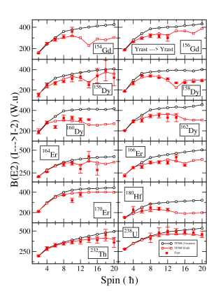
Figure 11: (Color online) $B(E2)$ transition probabilities (W.u) from yrast-band to the yrast-band for ^154,156Gd, ^{156,158,160,162}Dy, ^164,166,170Er, ¹⁸⁰Hf, ²³²Th and ²³⁸U isotopes. The black curves show the TPSM values for the vacuum configuration denoted by TPSM (Vacuum). The red curves show the TPSM values including the quasiparticle configuration denoted by TPSM (Full). The bold red squares show the experimental values (Data taken from Reich2009 ; Reich2012 ; Nica2017 ; Nica2021 ; Reich2007 ; Singh2018 ; Baglin2008 ; Baglin2018 ; Wu2003 ; Browne2006 ; Martin2002 ).

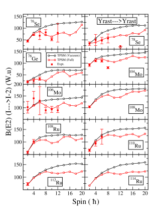
Figure 12: (Color online) $B(E2)$ transition probabilities (W.u) from yrast-band to the yrast-band for ^76,78Se, ⁷⁶Ge, ^104,106,108Mo and ^{108,110,112,114}Ru isotopes. The black curves show the TPSM values for the vacuum configuration denoted by TPSM (Vacuum). The red curves show the TPSM values including the quasiparticle configuration denoted by TPSM (Full). The bold red squares show the experimental values (Data taken from Singh1984 ; Farhan2009 ; Blach2007 ; Fren2008 ; Blach2000 ; Gurdal2012 ; Lalkov2015 ).

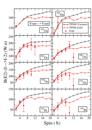
Figure 13: (Color online) $B(E2)$ transition probabilities (W.u) from yrast-band to the yrast-band for ^182-192Os and ^192,194Pt isotopes. The black curves show the TPSM values for the vacuum configuration denoted by TPSM (Vacuum). The red curves show the TPSM values including the quasiparticle configuration denoted by TPSM (Full). The bold red squares show the experimental values (Data taken from Singh2015 ; Baglin2010 ; Baglin2003 ; Singh2002 ; Singh190 ; Baglin2012 ; Chen194 ).

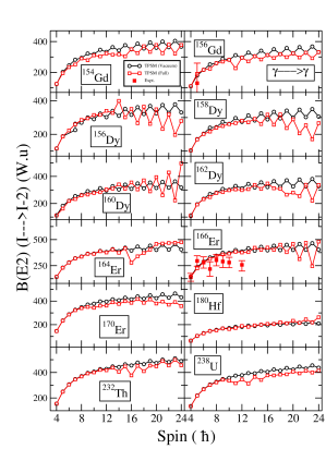
Figure 14: (Color online) $B(E2)$ transition probabilities (W.u) from $\gamma$-band to the $\gamma$-band for ^154,156Gd, ^{156,158,160,162}Dy, ^164,166,170Er, ¹⁸⁰Hf, ²³²Th and ²³⁸U isotopes. The black curves show the TPSM values for the vacuum configuration denoted by TPSM (Vacuum). The red curves show the TPSM values including the quasiparticle configuration denoted by TPSM (Full). The bold red squares show the experimental values (Data taken from Reich2009 ; Reich2012 ; Nica2017 ; Nica2021 ; Reich2007 ; Singh2018 ; Baglin2008 ; Baglin2018 ; Wu2003 ; Browne2006 ; Martin2002 ).

Figure 15: (Color online) $B(E2)$ transition probabilities (W.u) from $\gamma$-band to the $\gamma$-band for ^76,78Se, ⁷⁶Ge, ^104,106,108Mo and ^{108,110,112,114}Ru isotopes. The black curves show the TPSM values for the vacuum configuration denoted by TPSM (Vacuum). The red curves show the TPSM values including the quasiparticle configuration denoted by TPSM (Full). The bold red squares show the experimental values (Data taken from Singh1984 ; Farhan2009 ; Blach2007 ; Fren2008 ; Blach2000 ; Gurdal2012 ; Lalkov2015 ).

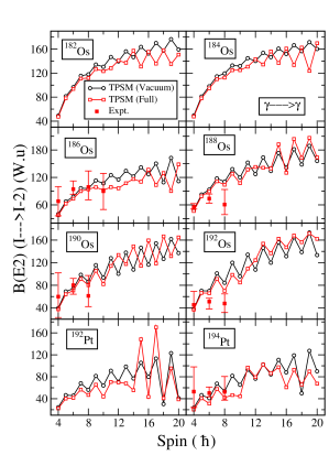
Figure 16: (Color online) $B(E2)$ transition probabilities (W.u) from $\gamma$-band to the $\gamma$-band for ^182-192Os and ^192,194Pt isotopes. The black curves show the TPSM values for the vacuum configuration denoted by TPSM (Vacuum). The red curves show the TPSM values including the quasiparticle configuration denoted by TPSM (Full).The bold red squares show the experimental values (Data taken from Singh2015 ; Baglin2010 ; Baglin2003 ; Singh2002 ; Singh190 ; Baglin2012 ; Chen194 ).

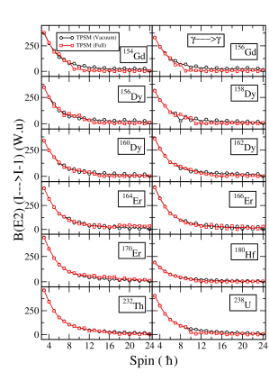
Figure 17: (Color online) $B(E2)$ transition probabilities (W.u) from $\gamma$-band to the $\gamma$-band for ^154,156Gd, ^{156,158,160,162}Dy, ^164,166,170Er, ¹⁸⁰Hf, ²³²Th and ²³⁸U isotopes. The black curves show the TPSM values for the vacuum configuration denoted by TPSM (Vacuum). The red curves show the TPSM values including the quasiparticle configuration denoted by TPSM (Full).

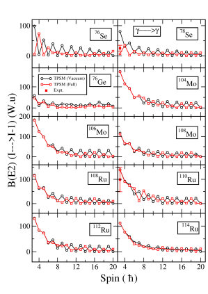
Figure 18: (Color online) $B(E2)$ transition probabilities (W.u) from $\gamma$-band to the $\gamma$-band for ^76,78Se, ⁷⁶Ge, ^104,106,108Mo and ^{108,110,112,114}Ru isotopes. The black curves show the TPSM values for the vacuum configuration denoted by TPSM (Vacuum). The red curves show the TPSM values including the quasiparticle configuration denoted by TPSM (Full). The bold red squares show the experimental values (Data taken from Singh1984 ; Farhan2009 ; Blach2007 ; Fren2008 ; Blach2000 ; Gurdal2012 ; Lalkov2015 ).

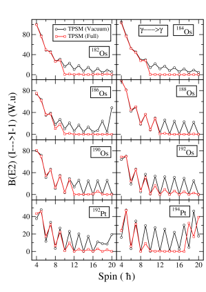
Figure 19: (Color online) $B(E2)$ transition probabilities (W.u) from $\gamma$-band to the $\gamma$-band for ^182-192Os and ^192,194Pt isotopes. The black curves show the TPSM values for the vacuum configuration denoted by TPSM (Vacuum). The red curves show the TPSM values including the quasiparticle configuration denoted by TPSM (Full).

4 Discussion of the Results

As already stated in the introduction, the main objective of the present work is to evaluate the robustness of the TPSM approach to account for the features associated with triaxiality and $\gamma$-softness of the collective Bohr Hamiltonian, discussed in the preceding section. As a first step, some basic properties of the rotational bands are analyzed. In Table 3, the energies of the 2${}^{+}_{1}$, $4^{+}_{1}$ and $2^{+}_{2}$ states along with the transition probabilities $B(E2,2^{+}_{1}\rightarrow 0^{+}_{1})$ and $B(E2,2^{+}_{2}\rightarrow 0^{+}_{1})$ are listed. The model parameters $\epsilon$ for the thirty nuclei are mostly adopted from our earlier works GH14 ; GH08 ; bh15 ; GS12 ; SJ21 . These values are slightly adjusted from the empirical values of Raman et al. raman to reproduce the $B(E2,2^{+}_{1}\rightarrow 0^{+}_{1})$ transition probability in the TPSM approach. In our earlier works, we focused on the excitation energies, and no adjustment to reproduce $B(E2,2^{+}_{1}\rightarrow 0^{+}_{1})$ was performed. On the other hand, the $\epsilon^{\prime}$ parameters, listed in Table 3, are adjusted to reproduce the band head energy of the $\gamma$-band, $E(2^{+}_{2})$. It is evident from Table 3 that the experimental energies of the $E(2^{+}_{1})$ states, which are model predictions, are very well reproduced. The experimental data on $B(E2,2^{+}_{2}\rightarrow 0^{+}_{1})$ transition probabilities from the head of the $\gamma$- to the yrast-bands are less complete and accurate. The TPSM results agree within the error bars with the experiment values. The experimental error bars for Os- and Pt- isotopes are too large to make a proper assessment of the predicted values. In the following subsections, we turn our attention to various measured properties of near-yrast rotational bands of the thirty isotopes studied in the present work.

4.1 Relation between Gamma-Rotor and TPSM

In Section 2, we discussed how the staggering pattern emerge as a consequence of the interaction of the even-$I$-states of harmonic $\gamma$-band with the states of the ground-band and the states of the $0^{+}_{2}$ band based on the harmonic $\gamma\gamma 0$ nature. This excitation has a pulsating nature, that is, it represents a collective motion between prolate and oblate via triaxial shapes. Obviously the admixture of such a mode is a measure of $\gamma$-softness.

As the TPSM is based on a mean-field with a fixed triaxial deformation, it does not incorporate such a collective excitations in an explicit way. It only contains the $0^{+}_{1},~{}2^{+}_{2},~{}4^{+}_{3},~{}...$ bands, which are generated by projecting the sequences of intrinsic states $K=0$, $K=2$, $K=4,~{}...$ from the triaxial quasiparticle vacuum state. In addition projected two- and four-quasiparticle states are taken into account. The TPSM staggering pattern is generated by the energy shifts caused by the mixing of the $K=2$ and $K=0$ vacuum bands and of the quasiparticle bands, where two-quasiparticle configurations generated from high-j orbitals $i_{13/2}$, $h_{11/2}$ and $f_{7/2}$ play the decisive role. As for the phenomenological Gamma-rotor, the competition between the two kinds of admixtures decides which pattern prevails. We discuss examples of the TPSM band mixing in section 4.7. More examples can be found in Refs. GH14 ; SJ21 ; Na23 ; SPRTBP .

The states of the TPSM without quasiparticle admixtures always generate the even-$I$-up pattern because of the repulsion between the even-$I$-states of the $K=0$ and $K=2$ bands. The pattern of even-$I$-up can be associated with a narrow Gamma-rotor potential that has a minimum at $\gamma_{m}>0$ and a $\gamma\gamma 0$-band at large energy. The amplitude of $S(I)$ is substantially smaller than it is for a rotor with irrotational-flow moments of inertia that corresponds to the $\gamma$-deformation of the TPSM calculation. For instance, see $S(I)$ without quasiparticle admixtures in Fig. 10 for ¹⁹²Pt where the TPSM assumes $\gamma_{N}\approx 30^{\circ}$. According to Eq. (26), the triaxial rotor amplitude of $S(I)$ is $I-4.5$ while the TPSM amplitude is approximately $0.1(I-4.5)$. A similar or even stronger reduction of the amplitude is noted for the other nuclides in Fig. 10 and the Ru isotopes in Fig. 9 for which the TPSM assumes $\gamma\approx 30^{\circ}$.

Microscopic calculations of the moments of inertia of the three principal axes by means of the cranking model give ratios of the moments of inertia that are not very different from the irrotational-flow ratios Frauendorf18 , which implies that the triaxial rotor model with cranking moments of inertia will give $S(I)$ values that are comparable with the large values obtained from Eq. (26). Thus the reduction must have a different origin. In contrast to the triaxial rotor model, the orientation angles of the deformed mean-field of the TPSM are not sharp. The overlap between a mean-field state and the same state rotated by an angle $\psi$ has a finite width $\Delta\psi$. In Refs. SF01 ; SF18 , the author has called $\Delta\psi$ the "coherence angle" and discussed its relation with the appearance and termination of rotational bands. In the framework of the TPSM, the finite coherence angle is reflected by the non-orthogonality of the different $K$ components projected from one and the same mean-field configuration and leads to a modified matrix in the $K$-space as compared to the one of the triaxial rotor model. The TPSM matrix generates qualitatively the same spectrum as the triaxial rotor, consisting of ground-band , $\gamma$-band, $\gamma\gamma 4$-band, etc. Quantitatively the energies and transition rates differ from the triaxial rotor model one’s.

4.2 Energies

The energies of the $I=2$ heads of the $\gamma$-bands are input in the TPSM calculations. All other energies are calculated. The resulting TPSM ratios $E(2^{+}_{2})/E(2^{+}_{1})$ and $E(2^{+}_{2})/E(4^{+}_{1})$ ratios in Table 3 compare well with the experimental ones. The deviations are caused by the $E(2^{+}_{1})$ and $E(4^{+}_{1})$ energies, which the TPSM tends to slightly overestimate.

Figs. 4, 5 and 6 show the angular momentum as function of the angular frequency, defined as

$$\omega(I)=(E(I)-E(I-2))/2~{}~{}\mathrm{associated~{}with}~{}~{}I-1/2.$$ (23)

It is evident from the figures that TPSM results are in good agreement with the experimental numbers. The energies of some of the isotopes have already been reported in our earlier publications GH14 ; SJ18 ; SJ21 . At the frequency of 0.3-0.4 MeV the ground-band interacts with the s-band, which is a superposition of high-j two-quasiparticle configurations. The phenomenon, seen as an up-bend or back-bend, has been extensively discussed in the literature (see, e.g., SJ18 ; SF01 ; SF18 ). The crossing frequency is systematically reproduced. The curvature of the crossing depends sensitively on the position of the Fermi level, which has the consequence that it is difficult to reproduce.

The TPSM calculations predict that $\gamma$-band crosses the two-quasiparticle bands at about the same frequency as the g-band. The structure of the mixed state has not been studied yet in a systematic way (see Ref. SJ18 for ¹⁵⁶Dy). In most nuclides, the $\gamma$-bands are not observed high enough to compare with the TPSM calculations. In cases that allow a comparison, the TPSM describes well the $\gamma$-band crossing as well as the crossing of the ground-band with the s-band.

The calculated energies have been used to evaluate the staggering parameter of the $\gamma$-bands. The values of $\bar{S}(6)$ are listed in Table 3. Figs. 7-10 display $S(I)$ over an extended spin range. The table and the figures demonstrate how well the TPSM calculations account for the experimental values. The amplitude of $S(I)$ becomes large when the $\gamma$-band enters the region of the two-quasiparticle bands which is seen as the up- or back- bends in Figs. 4, 5 and 6 (c.f. Sec. 4.7).

The isotopes of Gd, Dy, Er, Th and U have large ratios of $E(2^{+}_{2})/E(4^{+}_{1})$ which are expected for prolate shape and near harmonic $\gamma$-vibrations. Accordingly, the staggering pattern in Fig. 7, $S(I)$ is very weak, which is reproduced by the TPSM calculations. The only exceptions are ¹⁷⁰Er and ²³²Th, which show a substantial even-$I$-up pattern associated with triaxiality. The TPSM provides the even-$I$-up staggering for ²³²Th though too weak. The discrepancies for ¹⁷⁰Er in Table 3 and Fig. 8 reflect the presence of a low-lying $\Delta I=2$ band, which is not accounted for by the TPSM. The nature of this band is beyond the scope of the present work.

In Table 3, Se-, Ge-, Mo-, Ru-, and Pt-isotopes have ratios of $E(2^{+}_{2})/E(4^{+}_{1})$ around one or lower, indicative of a large triaxiality. The TPSM reproduces the positive value of $\bar{S}(6)$ for ⁷⁶Ge, which implies more rigid triaxiality. The TPSM does not describe the experimental staggering pattern of ⁷⁶Se, whereas it accounts for the even-$I$-down staggering of ⁷⁸Se. The even-$I$-down pattern of the Mo-isotopes is reproduced by the TPSM, though with a large amplitude.

The transition from the even-$I$-down to the even-$I$-up pattern seen in the Ru-isotopes is present in the TPSM values, although $\bar{S}(6)$ changes sign two neutrons early ($\bar{S}(6)=-0.15$ for ¹⁰⁴ Ru), while the other indicators ${\left[\frac{E(2^{+}_{2})}{E(2^{+}_{1})}\right]}$, ${\left[\frac{E(2^{+}_{2})}{E(4^{+}_{1})}\right]}$ do not change much along the isotope chain $\biggl{(}{\left[\frac{E(2^{+}_{2})}{E(2^{+}_{1})}\right]}$=2.5, ${\left[\frac{E(2^{+}_{2})}{E(4^{+}_{1})}\right]}$=1.0 for ¹⁰⁴Ru$\biggl{)}$. This indicates that the shell structure of the orbits near the Fermi level plays a significant role in the $N$-dependence of $\bar{S}(6)$, because the three characteristics are much stronger correlated in Gamma-rotor model.

The $\bar{S}(6)$ values in the chain of the Os-isotopes is reasonably well accounted for by the TPSM. The changes in other indicators : ${\left[\frac{E(2^{+}_{2})}{E(2^{+}_{1})}\right]}$, ${\left[\frac{E(2^{+}_{2})}{E(4^{+}_{1})}\right]}$ does not correlate with the $N$-dependence of $\bar{S}(6)$ as expected form the Gamma-rotor model, which points to the influence of the shell structure.

Table 1 suggests to associate the Gd-, Dy-, Er-, Th- and U-isotopes with prolate potentials of the 200-0 class. However, it seems impossible to find a potential that accounts for both the large $E(2^{+}_{2})/E(4^{+}_{1})$ ratios and the substantial even-$I$-up staggering in ¹⁷⁰Er and ²³²Th. The remaining nuclides can be associated with soft potentials somewhere between 50-30, 50-50, 0-20 and 50-0. It seems inappropriate to claim "evidence for rigid triaxial deformation at low energy in ⁷⁶Ge" Toh13 . The amplitude of $S(I)$ and the small ratio $B(E2,2^{+}_{2}\rightarrow 0^{+}_{1})/B(E2,2^{+}_{1}\rightarrow 0^{+}_{1})$ rather suggest a soft triaxial potential of the type 0-30 between 0-20 and 0-50.

4.3 In-band $B(E2)$ transitions

Figs. 11, 12 and 13 depict the $B(E2,I\rightarrow I-2)$ values for the transitions between the states of the yrast-bands. The TPSM calculations without quasiparticle admixtures result in a smooth I dependence, as expected. The results with full the basis give a drop in the $B(E2)$ values at higher spin, which reflects the crossing between the ground- and the s-band. The latter is composed of two rotational aligned high-j quasiparticles, which reduce the $B(E2,I\rightarrow I-2)$ value. Above the crossing, the yrast line is composed of the s-band, and the full TPSM results are below the vacuum only values. The fact that the band crossing seen in the $I(\omega)$ plots of Figs. 4, 5 and 6 is accompanied by a drop in the $B(E2,I\rightarrow I-2)$ values has been discussed in the literature in connection with the back bending phenomenon (see, e.g., SJ18 ; SF01 ; SF18 ).

For the rare earth nuclei, the first crossing occurs around $I=12$, and the $B(E2,I\rightarrow I-2)$ values in Fig. 11 stay below the vacuum values above this spin. For ¹⁷⁰Er, ¹⁸⁰Hf, ²³²Th and ²³⁸U the transition probabilities in Fig. 11 do not display much of a reduction.

The calculated yrast $B(E2,I\rightarrow I-2)$ values transitions for ^76,78Se, ⁷⁶Ge, ^104,106,108Mo and ^{108,110,112,114}Ru are compared with the measured values in Fig. 12. The TPSM calculations with full basis show two drops. In this region the neutron and proton Fermi surfaces are very close. In most of the cases, two neutrons align first quickly followed by the alignment of two protons. It is evident from the figure that TPSM reproduces the measured values reasonably well. There are two measured transitions, one for ⁷⁶Se at $I=8$ and the other for ¹⁰⁴Mo at $I=12$ that deviate from the expected trend and from the predicted TPSM values. These large deviations indicate the presence of shape isomeric states for these nuclei Moller2009 . This is to remind that TPSM approach projects the good angular momentum states from one and the same mean-field. The truncated multi-quasiparticle basis (3) is too restricted to accommodate such a drastic change of the deformation. Similarly, the drastic drop of the experimental $B(E2,I\rightarrow I-2)$ values at $I=10$ seen in Fig. 13 for the heavy Os- and Pt- isotopes is not reproduced by the TPSM calculations. The discrepancy seems to indicate that the crossing s-band has a different mean-field deformation, which the TPSM calculations cannot account for.

Table 4: Mixing ratios for the inter-band $2_{2}\rightarrow 2_{1}$ and intra-band $3_{1}\rightarrow 2_{2}$ transitions given by expression $\delta=0.835E_{\gamma}\frac{\langle J_{f}||\mathcal{M}(E2)||J_{i}\rangle}{\langle J_{f}||\mathcal{M}(M1)||J_{i}\rangle}$. The experimental values are in parenthesis with error bars in curly brackets (Data taken from Krane1974 ; Chung1970 ; Grab1960 ; Lieder1970 ; Eldri2018 ; Uluert2018 ; Kraci1998 ; Domi1972 ).

Isotope	$2_{2}\rightarrow 2_{1}$	$3_{1}\rightarrow 2_{2}$	Isotope	$2_{2}\rightarrow 2_{1}$	$3_{1}\rightarrow 2_{2}$	Isotope	$2_{2}\rightarrow 2_{1}$	$3_{1}\rightarrow 2_{2}$
	(Expt.)	(Expt.)		(Expt.)	(Expt.)		(Expt.)	(Expt.)
76Ge	2.099	0.479	154Gd	-34.174	1.587	182Os	45.917	1.736
	(3.5 {15})
76Se	6.228	0.176	156Gd	-8.27	2.376	184Os	22.549	1.265
	(5.5 {5})			(-6.5 {${}^{+2.6}_{-7.9}$})
78Se	6.299	0.209	156Dy	-9.837	0.977	186Os	33.968	3.627
	(6 {${}^{+7}_{-2}$})
104Mo	10.383	0.552	158Dy	-10.967	1.174	188Os	22.549	4.401
	(9 {${}^{+4}_{-2}$})
106Mo	7.841	0.749	160Dy	-16.634	1.861	190Os	20.513	7.958
	(6.2 {${}^{+1}_{-8}$})			(-12.5 {${}^{+2.9}_{-5.0}$})
108Mo	19.745	0.521	162Dy	-6.65	8.449	192Os	-18.895	0.398
	(23 {${}^{\infty}_{-14}$})			($\geq 29$)
108Ru	14.809	0.489	164Er	23.804	2.369	192Pt	2.617	1.147
	(16 {${}^{+9}_{-4}$})
110Ru	1.1402	0.508	166Er	42.889	1.03	194Pt	5.644	3.022
	($\infty\{^{>50}_{<-75}\}$)			(38 {${}^{\infty}_{-24}$})
112Ru	-27.363	0.466	170Er	56.622	4.327	232Th	56.948	3.537
	(-30 {${}^{+10}_{-31}$})			(57 {${}^{\infty}_{-41}$})
114Ru	-6.225	0.447	180Hf	25.568	0.793	238U	25.62	1.771

Table 5: The TPSM and experimental values (experimental values are in parentheses with error bars in curly brackets) of static quadrupole moments $Q=\sqrt{\frac{32\pi}{175}}\langle I=2,M=2|\mathcal{M}(\textrm{E}2)|I=2,M=2\rangle$and g factors for thirty nuclei. (Data taken from NNDC ; Ayangeakaa2019 ; Wu1996 ; Allmond2008 ; Corm2019 ; Smith2004 ; Menzen1985 ; Bao2007 )

Isotope	$Q_{2^{+}_{1}}$	$Q_{2^{+}_{2}}$	g${}_{2^{+}_{1}}$	Isotope	$Q_{2^{+}_{1}}$	$Q_{2^{+}_{2}}$	g${}_{2^{+}_{1}}$	Isotope	$Q_{2^{+}_{1}}$	$Q_{2^{+}_{2}}$	g${}_{2^{+}_{1}}$
	(Expt.)	(Expt.)	(Expt.)		(Expt.)	(Expt.)	(Expt.)		(Expt.)	(Expt.)	(Expt.)
76Ge	-0.179	0.188	0.238	154Gd	-1.719	1.719	0.345	182Os	-1.382	1.375	0.263
	(-0.181)	(0.197)	(0.263 {21})		(-1.82 {4})		(0.48 {3})
76Se	-0.084	0.647	0.344	156Gd	-1.714	1.717	0.296	184Os	-1.415	1.407	0.271
	(-0.34 {7})		(0.350 {27})		(-1.93{4})		(0.41 {7})		(-2.4 {11})
78Se	-0.462	0.465	0.351	156Dy	-1.970	1.971	0.391	186Os	-1.212	1.203	0.261
	(-0,20 {7})	(0.17 {9})	(0.325 {24})				(0.39 {4})		(-1.326)	(1.203)	(0.26 {2})
104Mo	-1.022	1.019	0.220	158Dy	-1.885	1.883	0.347	188Os	-1.410	1.409	0.282
			(0.27 {2})				(0.36 {3})		(-1.311)	(1.408)	(0.29 {1})
106Mo	-1.076	1.075	0.241	160Dy	-1.987	1.984	0.381	190Os	-1.286	1.286	0.298
			(0.21 {2})		(-1.8 {4})		(0.35 {2})		(-0.947)	(1.285)	(0.35 {1})
108Mo	-0.852	0.854	0.275	162Dy	-2.063	1.063	0.292	192Os	-1.219	1.221	0.276
			(0.5 {3})				(0.35 {2})		(-0.916)	(1.221)	(0.40 {1})
108Ru	-0.811	0.816	0.267	164Er	-2.282	2.284	0.299	192Pt	-0.940	0.936	0.195
			(0.23 {4})		<0	(2.4 {3})	(0.349 {8})				(0.29 {2})
110Ru	-0.950	0.954	0.320	166Er	-2.321	2.324	0.275	194Pt	-0.635	0.635	0.176
	(-0.74 {9})		(0.44 {7})		(-1.9)	(2.2)	(0.325 {5})		(0.409)	(0.635)	(0.30 {2})
112Ru	-0.766	0.772	0.354	170Er	-2.365	2.364	0.287	232Th	-2.981	2.991	0.287
			(0.44 {9})		-1.94 {23})	(2.0 {3})	(0.317 {7})
114Ru	-0.663	0.669	0.353	180Hf	-1.621	1.616	0.251	238U	-2.851	2.850	0.281
					(-2.00 {2})		(0.31 {2})

Table 6: The TPSM energies and B(E2) transition probabilities (W.u) of $0_{2}^{+}$ band for thirty nuclei. The experimental values are in parenthesis with error bars are in curly brackets (Data taken from Farhan2009 ; Reich2009 ; Reich2012 ; Nica2017 ; Nica2021 ; Singh2018 ; Baglin2008 ; Baglin2018 ; Singh2002 ; Singh190 ; Baglin2012 ; Chen194 ; Browne2006 ; Martin2002 ).

Isotope	Energy	Energy	Energy	B(E2)	B(E2)	B(E2)	B(E2)	B(E2)
	$0^{+}_{2}$	$2^{+}_{3}$	$4^{+}_{3}$	$0_{2}\rightarrow 2_{1}$	$0_{2}\rightarrow 2_{2}$	$2_{3}\rightarrow 0_{1}$	$4_{3}\rightarrow 2_{1}$	$4_{3}\rightarrow 2_{2}$
76Ge	1.902 (1.911)	2.622 (2.504)	2.890 (2.733)	1.639	2.277	0.143	0.569	12.456
76Se	1.164 (1.122)	1.612 (1.787)	1.905	148.723	3.957	0.061	0.724	2.402
78Se	1.482 (1.498)	1.828 (1.995)	2.266	2.031 (1.17 {21})	0.152	0.087 (0.09 {+3,-6})	0.176	9.320
104Mo	0.901 (0.886)	1.000	1.227	1.914	0.004	0.076	0.002	15.972
106Mo	0.895 (0.957)	0.971	1.259	0.079	0.318	0.058	0.052	0.009
108Mo	1.036	1.170	1.441	0.513	2.307	0.163	0.243	0.002
108Ru	0.948 (0.976)	1.062	1.303	29.614	0.109	0.074	0.310	0.003
110Ru	1.136 (1.137)	1.358 (1.396)	1.571	249.135	0.041	0.007	0.003	0.540
112Ru	1.126	1.251	1.483	67.496	0.001	0.001	0.557	16.247
114Ru	0.961	1.087	1.348	115.288	59.902	0.0401	0.363	18.857
154Gd	0.781 (0.681)	0.848 (0.815)	1.197 (1.048)	18.438 (52 {8})	18.397	3.046 (6.7 {6})	0.002	0.003
156Gd	0.989 (1.049)	1.15 (1.129)	1.304 (1.298)	11.731 (8 {+4,-7})	80.182	11.268	3.479 (1.3 {+5,-7})	0.376
156Dy	0.739 (0.676)	0.893 (0.829)	1.017 (1.088)	9.853	38.872	0.032	0.001	0.013
158Dy	0.956 (0.991)	1.008 (1.086)	1.130 (1.280)	6.889	47.854	0.081 (2.1 {5})	0.074	0.091
160Dy	1.254 (1.279)	1.315 (1.349)	1.576 (1.522)	1.025	7.861	0.086 (0.65 {8,7})	0.160	0.004
162Dy	1.333 (1.400)	1.383 (1.453)	1.488 (1.574)	1.164	0.003	0.01	0.004	0.041
164Er	1.214 (1.246)	1.377 (1.314)	1.424 (1.469)	0.354	5.236	0.055 (0.23 {12})	0.170	0.002
166Er	1.486 (1.460)	1.543 (1.528)	1.675 (1.679)	4.478 (2.7 {10})	1.438	0.032	0.091	8.93 (7.4 {25})
170Er	0.850 (0.890)	0.999 (0.960)	1.102 (1.103)	0.127	0.757	0.080 (0.28 {3})	0.026	0.133
180Hf	0.803 (1.102)	1.063 (1.183)	1.243	22.641	0.018	13.323	7.149	0.078
182Os	0.652	0.878	1.118	0.935	0.042	15.754	7.821	0.031
184Os	0.894 (1.042)	1.112 (1.204)	1.189 (1.506)	0.009	0.001	14.477	7.243	0.032
186Os	1.206 (1.061)	1.377 (1.208)	1.518 (1.461)	0.010	0.063	0.034	0.155	0.044
188Os	1.023 (1.086)	1.150 (1.304)	1.251	2.765 (0.95 {8})	2.213 (4.3 {5})	0.040	0.003	25.052
190Os	0.975 (0.912)	1.099 (1.114)	1.358	4.036 (2.4 {+8,-6})	0.012 (24 {10,-7})	0.049	0.011	23.242
192Os	0.719 (0.956)	0.811 (1.127)	1.039	0.682 (0.57 {12})	9.740 (30.04 {+30,-23})	0.004	0.022	21.411
192Pt	0.907 (1.195)	1.249 (1.439)	1.684	23.653	20.792	0.039	0.222	7.556
194Pt	1.182 (1.2672)	1.393	1.600	1.967 (0.63 {+20,-13})	3.463 (8.2 [+25, -16])	0.071	0.364	20.337
232Th	0.727 (0.731)	0.759 (0.774)	0.833 (0.873)	0.433	8.660	1.05 (2.9 {4})	1.01	7.165
238U	0.914 (0.927)	0.941 (0.996)	1.002 (1.056)	4.632	2.650	1.482 (0.38 {16})	6.164	1.048

The $B(E2,I\rightarrow I-2)$ values for the transitions within the $\gamma$-bands are displayed in Figs. 14, 15 and 16. As expected, the vacuum-only TPSM values increase steadily, which is overlaid by an even-$I$-up staggering pattern. The results of the full TPSM calculation agree with the vacuum only set for low spin states and fall below them for large spin. How staggering pattern changes is discussed in the following. The TPSM values agree reasonably well with the limited data.

Figs. 7 - 10 compare the staggering parameter $S(I)$ calculated by means of Eq. (1) from the energies of the $\gamma$-bands with the staggering parameter calculated by the analog equation (7) from the $B(E2,I\rightarrow I-2)$ values.

The $B(E2)$ staggering calculations without quasiparticle admixtures show even-$I$-down pattern, which is opposite to the even-$I$-up staggering of the $\gamma$-band energies. As we discussed in Sec. 4.1, the TPSM results without quasiparticle excitations show the qualitative features of the triaxial Gamma-rotor. In Sec. 2 we explain that the even-$I$-up pattern of energies reflects the mixing of the even-$I$-states of the $\gamma$-band with the ground-band and that the same mixing generates the reduction of the $B(E2,I\rightarrow I-2)$ values. Thus the opposite phase of the staggering of the $\gamma$-band energies and intra-band $B(E2,I\rightarrow I-2)$ values appears in a regular way.

As seen in Figs. 7-10, including the quasiparticle admixtures changes the $B(E2,I\rightarrow I-2)$ staggering pattern for a majority of nuclides as follows. When the admixtures do not change the energy staggering from even-$I$-up to even-I-down the $B(E2,I\rightarrow I-2)$ staggering remains even-$I$-down as well ( ⁷⁶Ge, ¹¹²Ru, ¹⁷⁰Er, ^182,188Os, ¹⁹²Pt and ²³²Th). When the admixtures reverse the energy staggering to even-$I$- down the $B(E2)$ staggering remains even-I-low for the low I values. Around $I=8$ to 10 the $B(E2,I\rightarrow I-2)$ staggering sets in with the phase opposite to the energy staggering, which becomes large. The change of the pattern is discussed in Sec. 4.7.

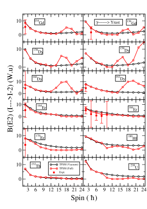
Figure 20: (Color online) $B(E2)$ transition probabilities (W.u) from $\gamma$-band to the yrast-band for ^154,156Gd, ^{156,158,160,162}Dy, ^164,166,170Er, ¹⁸⁰Hf, ²³²Th and ²³⁸U isotopes. The black curves show the TPSM values for the vacuum configuration denoted by TPSM (Vacuum). The red curves show the TPSM values including the quasiparticle configuration denoted by TPSM (Full). The bold red squares show the experimental values (Data taken from Reich2009 ; Reich2012 ; Nica2017 ; Nica2021 ; Reich2007 ; Singh2018 ; Baglin2008 ; Baglin2018 ; Wu2003 ; Browne2006 ; Martin2002 ).

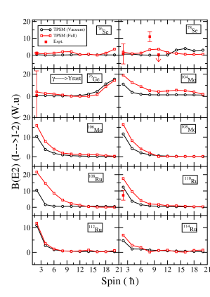
Figure 21: (Color online) $B(E2)$ transition probabilities (W.u) from $\gamma$-band to the yrast-band for ^76,78Se, ⁷⁶Ge, ^104,106,108Mo and ^{108,110,112,114}Ru isotopes. The black curves show the TPSM values for the vacuum configuration denoted by TPSM (Vacuum). The red curves show the TPSM values including the quasiparticle configuration denoted by TPSM (Full). The bold red squares show the experimental values (Data taken from Singh1984 ; Farhan2009 ; Blach2007 ; Fren2008 ; Blach2000 ; Gurdal2012 ; Lalkov2015 ).

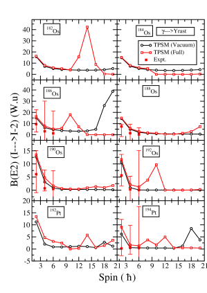
Figure 22: (Color online) $B(E2)$ transition probabilities (W.u) from $\gamma$-band to the yrast-band for ^182-192Os and ^192,194Pt isotopes. The black curves show the TPSM values for the vacuum configuration denoted by TPSM (Vacuum). The red curves show the TPSM values including the quasiparticle configuration denoted by TPSM (Full). The bold red squares show the experimental values (Data taken from Singh2015 ; Baglin2010 ; Baglin2003 ; Singh2002 ; Singh190 ; Baglin2012 ; Chen194 ).

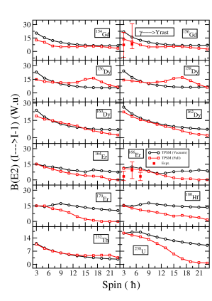
Figure 23: (Color online) $B(E2)$ transition probabilities (W.u) from $\gamma$-band to the yrast-band for ^154,156Gd, ^{156,158,160,162}Dy, ^164,166,170Er, ¹⁸⁰Hf, ²³²Th and ²³⁸U isotopes. The black curves show the TPSM values for the vacuum configuration denoted by TPSM (Vacuum). The red curves show the TPSM values including the quasiparticle configuration denoted by TPSM (Full). The bold red squares show the experimental values (Data taken from Reich2009 ; Reich2012 ; Nica2017 ; Nica2021 ; Reich2007 ; Singh2018 ; Baglin2008 ; Baglin2018 ; Wu2003 ; Browne2006 ; Martin2002 ).

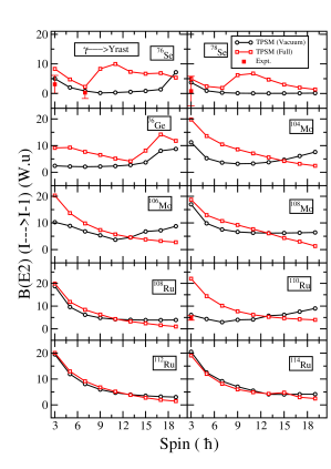
Figure 24: (Color online) $B(E2)$ transition probabilities (W.u) from $\gamma$-band to the yrast-band for ^76,78Se, ⁷⁶Ge, ^104,106,108Mo and ^{108,110,112,114}Ru isotopes. The black curves show the TPSM values for the vacuum configuration denoted by TPSM (Vacuum). The red curves show the TPSM values including the quasiparticle configuration denoted by TPSM (Full). The bold red squares show the experimental values (Data taken from Singh1984 ; Farhan2009 ; Blach2007 ; Fren2008 ; Blach2000 ; Gurdal2012 ; Lalkov2015 ).

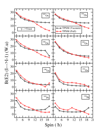
Figure 25: (Color online) $B(E2)$ transition probabilities (W.u) from $\gamma$-band to the yrast-band for ^182-192Os and ^192,194Pt isotopes. The black curves show the TPSM values for the vacuum configuration denoted by TPSM (Vacuum). The red curves show the TPSM values including the quasiparticle configuration denoted by TPSM (Full).

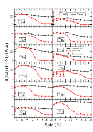
Figure 26: (Color online) $B(E2)$ transition probabilities (W.u) from $\gamma$-band to the yrast-band for ^154,156Gd, ^{156,158,160,162}Dy, ^164,166,170Er, ¹⁸⁰Hf, ²³²Th and ²³⁸U isotopes. The black curves show the TPSM values for the vacuum configuration denoted by TPSM (Vacuum). The red curves show the TPSM values including the quasiparticle configuration denoted by TPSM (Full). The bold red squares show the experimental values (Data taken from Reich2009 ; Reich2012 ; Nica2017 ; Nica2021 ; Reich2007 ; Singh2018 ; Baglin2008 ; Baglin2018 ; Wu2003 ; Browne2006 ; Martin2002 ).

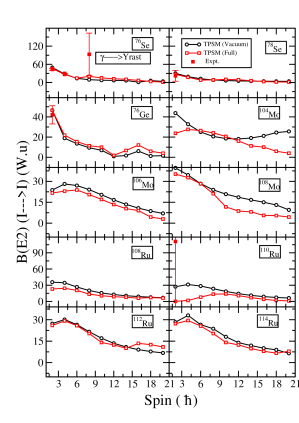
Figure 27: (Color online) $B(E2)$ transition probabilities (W.u) from $\gamma$-band to the yrast-band for ^76,78Se, ⁷⁶Ge, ^104,106,108Mo and ^{108,110,112,114}Ru isotopes.The black curves show the TPSM values for the vacuum configuration denoted by TPSM (Vacuum). The red curves show the TPSM values including the quasiparticle configuration denoted by TPSM (Full). The bold red squares show the experimental values (Data taken from Singh1984 ; Farhan2009 ; Blach2007 ; Fren2008 ; Blach2000 ; Gurdal2012 ; Lalkov2015 ).

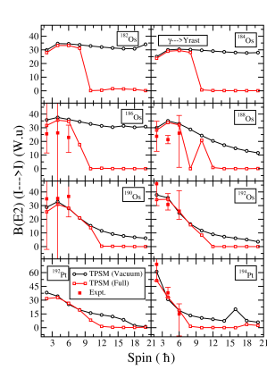
Figure 28: (Color online) $B(E2)$ transition probabilities (W.u) from $\gamma$-band to the yrast-band for ^182-192Os and ^192,194Pt isotopes. The black curves show the TPSM values for the vacuum configuration denoted by TPSM (Vacuum). The red curves show the TPSM values including the quasiparticle configuration denoted by TPSM (Full). The bold red squares show the experimental values (Data taken from Singh2015 ; Baglin2010 ; Baglin2003 ; Singh2002 ; Singh190 ; Baglin2012 ; Chen194 ).

The TPSM values $B(E2,I\rightarrow I-1)$ for the transitions between the $\gamma$-band states are shown in Figs. 17-19. For the calculations without quasiparticle admixtures, the phase of $S(I)$ is opposite to the phase of $S(I)$ of the energies like for the Gamma-rotor Hamiltonian (see Fig. 3). However, when the quasiparticle admixtures are taken into account there is no clear correlation between the phases of $S(I)$ from the energies and the $B(E2,I\rightarrow I-1)$. Comparison with experiment requires to take into account the competing $M1$ component, i. e., measuring the mixing ratios. However, to our knowledge there are no such data available.

4.4 Inter-band $B(E2)$ transition

Figs. 20 - 22 show the $B(E2,I\rightarrow I-2$) values for the transitions between the $\gamma$- and yrast-bands. The values for the $2^{+}_{2}\rightarrow 0^{+}_{1}$ transition are also listed in Table 3. The calculations agree well with the scarce data, which are too inaccurate to confirm the predicted decrease with angular momentum. Figs. 23 - 25 show the $B(E2,I\rightarrow I-1$) values for the transitions between the $\gamma$- and yrast-bands. The TPSM results again agree well with the only two data points available. Figs. 26 - 28 show the $B(E2,I\rightarrow I$) values for the transitions between the $\gamma$- and yrast-bands, which reproduce the data reasonably well. For many nuclei, the TPSM results for low-spin do not change appreciably when the quasiparticles are admixed, and the changes are less than the experimental errors. For the $\gamma$-soft nuclei of ^76,78Se, ⁷⁶Ge, ¹¹⁰Ru and ¹⁰⁴Ru Na23 , the quasiparticle admixtures are essential for reproducing the experimental values. This demonstrates in a way how the features of $\gamma$-softness come about in the TPSM framework. For the $I\rightarrow I-1$ and $I\rightarrow I$ transitions there is a $M1$ component. Table 4 lists the TPSM values of the inter-band $2_{2}\rightarrow 2_{1}$ and intra-band $3_{1}\rightarrow 2_{2}$ transitions, which agree with the limited experimental data within the large error bars.

4.5 Static moments

Table 5 lists the static quadrupole moments of the $2^{+}_{1}$ and $2^{+}_{2}$ states and the g factors of the $2^{+}_{1}$ states of the considered nuclei. The TPSM reproduces the data reasonably well for all the studied nuclei, except for the $Q$ values of ⁷⁸Se and the g-factors in ¹⁹²Os and ¹⁹⁴Pt. The TPSM reproduces the opposite signs of $Q$ found for the $2^{+}_{1}$ and $2^{+}_{2}$ states of the Gamma-rotor. It accounts for the small values of $|Q|$ in ⁷⁶Ge which are expected for $\gamma$ close to 30^∘.

4.6 Higher excitations

Table 6 lists the energies and $B(E2)$ values for the excited states that are central in the discussion of the nature of triaxiality. The structure of the low-energy spectrum of the collective Gamma-rotor Hamiltonian (3) is simple. It consists of the bands built on the states $0^{+}_{1}$ (ground), $2^{+}_{2}~{}(\gamma),~{}4^{+}_{3}~{}(\gamma\gamma 4)$ and $0^{+}_{2}~{}(\gamma\gamma 0)$. The TPSM spectrum is more complex, because it contains the states originating from the two- and four-quasiparticles, in addition. The $\gamma\gamma 4$-band, generated by $K=4$ projection from the quasiparticle vacuum, may have larger energy than a band built on a $K=4$ two-quasiparticle state. The nuclides with very small $B(E2,4^{+}_{3}\rightarrow 2^{+}_{2})$ transition probabilities are examples. The soft triaxial nuclei ^110,112Ru, ^188,190,192Os, and ¹⁹²Pt have the collective enhancement of  10-20 W.u., which is expected for a $\gamma\gamma 4\rightarrow\gamma$ transition.

Collectivity of the $\gamma\gamma 0$ type (pulsating shape) is not explicitly built into the TPSM. The collective enhancement of the $B(E2,0^{+}_{2}\rightarrow 2^{+}_{2})$ for several nuclides shows that the quasiparticle states admix in a coherent way to generate a collective state in the shell-model manner. However, the collective state must be more complex than the $\gamma\gamma 0$ pulsation because these $0^{+}_{2}$ states (except ¹⁹²Os) have collectively enhanced $B(E2,0^{+}_{2}\rightarrow 2^{+}_{1})$ probabilities, which are quenched for the purely collective $\gamma\gamma 0$ states of the Gamma-rotor (see Table 2). The diagonalization in the two- and four-quasiparticle space accounts also for the collective $\beta$ mode. The large values of $B(E2,0^{+}_{2}\rightarrow 2^{+}_{1})$ for the $N=90$, $92$ nuclei, ^154,156Gd and ^156,158Dy near the transition from small to large $\beta$ values are indications for this type of correlations. For the Os and Pt isotopes, which are close to the region of prolate-oblate shape coexistence, the transitions are collectively enhanced as well. In all cases, the TPSM generates collective enhancement of the $\beta$ type in a qualitative manner. However, the correlations between the quasiparticle excitations do not account in a quantitative way for the large-scale $\beta$ fluctuations in these nuclei.

For the prolate nuclei of ^160,162Dy, ^166,168,170Er and ¹⁸⁰Hf, the $B(E2,0^{+}_{2}\rightarrow 2^{+}_{1})$ and $B(E2,0^{+}_{2}\rightarrow 2^{+}_{2})$ values fluctuate. This seems to represent a transition from two-quasiparticle states with a varying amount of quadrupole-correlated admixtures. The interaction of the $\gamma$-band with these bands (and likely with higher $0^{+}_{3},~{}0^{+}_{4},~{}...$ bands) generates the weak even-$I$-down pattern seen in the energies for most of the prolate nuclei. It also explains its more erratic correlation with the staggering pattern of the intra $\gamma$-band $B(E2,I\rightarrow I-2)$. Most of the available data agree within the error bars with the TPSM results. However, there are very few measurements to test the TPSM predictions in a consistent manner.

4.7 Band mixing interpretation

In this section, we discuss how the triaxiality patterns of the TPSM results emerge using the band mixing argument. We address their changes with $N$ by comparing ¹⁸²Os with ¹⁸⁸Os. Additional analysis concerning ¹⁵⁶Dy, ¹⁰⁴Ru and ¹¹²Ru nuclides are given in Refs. SJ18 ; Na23 ; SPRTBP .

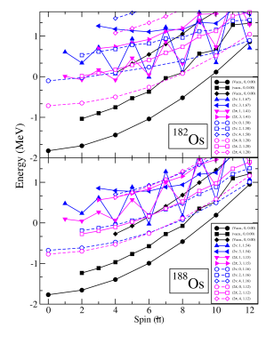
Figure 29: (Color online). Band diagrams for ^182,188Os showing the TPSM projected energies before band mixing. The bands are labelled by three quantities : quasiparticle character, $K$-quantum number and energy of the two-quasiparticle state. For instance, $(2\pi,~{}1,~{}1.40)$ in the upper panel designates the $K=1$ state projected from the $h_{11/2}$ two-quasiproton configuration with the energy of 1.40 MeV. The $K=0,~{}2,~{}4$ states projected from the quasiparticle vacuum are labelled with Vacu. The four-quasiparticle states lie above 2 MeV.).

The band diagram in Fig. 29 shows the energies of the projected quasiparticle configurations in ¹⁸²Os. Around $I=12$, the $K=1$ two-quasineutron configuration crosses the $K=0$ vacuum configuration, which causes the back bending anomaly of the yrast states. At such high spin, the $K$ of the two-quasineutron configuration is no longer approximately conserved, which results in a complex picture. To present the physics more clearly, Fig. 30 presents a modified band diagram, which shows the $h_{11/2}$ two-quasiproton and of the $i_{13/2}$ two-quasineutron bands after diagonalizing the TPSM Hamiltonian within their individual subspaces. The lowest two-quasiparticle $(2\nu,~{}1,~{}1.76)$ band with even $I$, which is commonly called the s-band, carries an additional angular moment of 8 compared the ground-band. It can be seen in Fig. 30 by comparing the angular momenta of the ground- and s-band at the same rotational frequency, which is the slope $E(I)$.

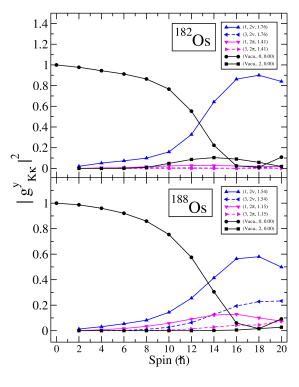
Figure 31: (Color online). Probabilities (18) of the pre-diagonalized high-j two-quasiparticle configurations in Fig. 30 for the yrast-bands in ^182,188Os.

Fig. 31 shows the probabilities $(g^{y})^{2}$ of the important components of the yrast-bands. The structural change from vacuum to the neutron s-band, which causes the back-bend in Fig. 6, is clearly seen. Compared to ¹⁸²Os, the structural change in ¹⁸⁸Os is more gradual and involves both the $(2\nu,~{}1,~{}1.54)$ and $(2\nu,~{}3,~{}1.54)$ bands. This is reflected by the later and smoother up-bend in Fig. 6.

Fig. 32 shows the $B(E2,I\rightarrow I-2)$ values between the states $I,~{}K=1$ projected from the two-quasineutron configuration at 1.67 MeV and the two-quasiproton configuration at 1.41 MeV. The intra-band $B(E2,I\rightarrow I-2)$ values for neutron s-band in Fig. 32 change from 150 W.u. at $I=12$ to 180 W.u. at $I=20$. As seen in Fig. 13, this accounts well for the reduced $B(E2,I\rightarrow I-2)$ values in the yrast sequence between 150 W.u and 160 W.u. in the same $I$ range. The systematic reduction of the $B(E2,I\rightarrow I-2)$ values in the yrast sequence of the other nuclides is explained in the same way by the crossing of the ground-band with the neutron s-band, which has smaller $B(E2,I\rightarrow I-2)$ values.

Fig. 33 illustrates the band mixing when the basis is truncated to the projected vacuum state only. It displays the probabilities of the $K=0$ and $K=4$ components admixed to the $K=2$ configuration after diagonaliztion within the truncated space. The admixture of the $K=0$ ground-band generates an upward shift of the even-$I$ states of the $\gamma$-band, which is seen in Fig. 10 "without quasiparticles". The downward shift by the $K=4$ band, which is about the same for even and odd $I$, does not change the staggering pattern. The upward shift is given by $H_{20}\times g^{\gamma}_{K=0,vac}$, where $H_{20}$ is the coupling matrix element. It is linear in the mixing amplitude $g^{\gamma}_{K=0,vac}$, which is reflected by the gradual increase of the staggering amplitude with $I$.

The intra-band $B(E2,I_{\gamma}\rightarrow I_{\gamma}-2)$ transitions "without quasiparticles" in Fig. 10 show a staggering which has a phase that is opposite to the energy staggering $S(I)$. The reason is the same as for the analog phase flip seen for the Gamma-rotor (c.f. Fig. 3) and is explained in the Appendix. It is proportional to the amplitude of the $K=0$ ground-band admixture and the quadrupole matrix element between $K=0$ and $K=2$, which explains the gradual increase of the staggering amplitude. The opposite staggering phase is a consequence of the relative phases of the amplitudes and the matrix element (see the discussion at the end of the Appendix).

Fig. 34 shows the composition of the $\gamma$-bands when all quasiparticle configurations are taken into account. The important admixtures are $(2\nu,~{}1,~{}1.76)$ and $(2\nu,~{}3,~{}1.76)$. Above $I$=12 these states dominate the wave function. The consequences of the structural change are complex. In the case of ¹⁸²Os, Fig. 16 indicate a reduction of the $B(E2,I_{\gamma}\rightarrow I_{\gamma}-2)$ values below the vacuum values, which is expected from Fig. 32 for the dominating two-quasineutron components in analogy to the yrast-band. However for ¹⁸⁸Os there is no such reduction. The reason is a mutual cancelation of the contributions from the $(2\nu,~{}1,~{}1.54)$ and $(2\nu,~{}3,~{}1.54)$ bands.

As seen in Fig. 10, below $I$=12 the staggering of the $B(E2)$ values does not change much when the coupling to quasiparticles is taken into account. The quasiparticle contributions are proportional to the square of the mixing amplitude because the quadrupole matrix elements between the vacuum and the two-quasineutron configuration are negligibly small. In contrast, the energy shifts are linear in the mixing amplitudes, and the modification of the energy staggering sets in already below $I$=12. The way the pattern changes is complex because the $(2\nu,~{}1,~{}1.76,~{}1,54)$, $(2\nu,~{}3,~{}1.67,~{}1.76)$ and the $K=0$ and 2 vacuum bands, and their mutual coupling matrix elements are involved.

Comparing the band diagrams in Fig. 30, the following difference is noticed. The neutron s-band $(2\nu,~{}1,~{}1,54,~{}I~{}even)$ in ¹⁸⁸Os encounters the $K=0$ vacuum band later and more gradually than the s-band $(2\nu,~{}1,~{}1,76,~{}I~{}even)$ in ¹⁸²Os, and the distance between the $K=0$ and 2 vacuum bands is smaller in ¹⁸²Os than in ¹⁸²Os. One may surmise that this results in a strong mixing of the bands in ¹⁸⁸Os and cancellation of the two-quasineutron components, whereas in ¹⁸²Os the mixing is weaker such that downward push by the s-band $(2\nu,~{}1,~{}1,76,~{}I~{}even)$ prevails for $I<12$ and changes the staggering phase. Fig. 6 reflects the differences by showing a later smooth up-bend for the former compared to the earlier sharp back-bend for the latter, which supports the interpretation. The same scenario is found in the Ru isotopes SJ21 ; Na23 ; SPRTBP . The band diagrams for ¹⁰⁴Ru and ¹¹²Ru show the analog differences as the ones for ¹⁸²Os and ¹⁸⁸Os. The even-$I$-down of $\gamma$-softness accompanied by a sharp back-bend is found in ¹⁰⁴Ru Na23 . The even-$I$-up of $\gamma$-rigidity accompanied by a smooth up-bend is found in ¹¹²Ru SJ21 .

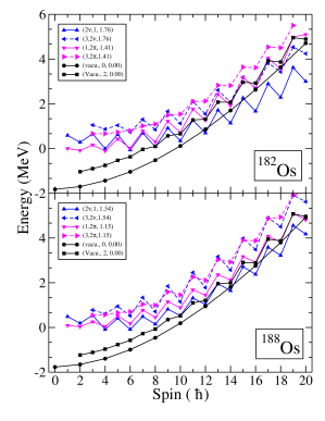
Figure 30: (Color online). Band diagrams for ^182,188Os after separate pre-diagonalization of the proton $h_{11/2}$ and neutron $i_{13/2}$ two-quasiparticle configurations. The states are labelled by their structure at $I=1,~{}2$, where they are not yet mixed. See Fig. 29 for details.

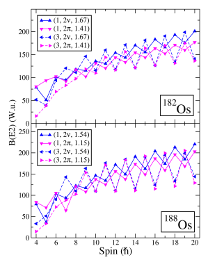
Figure 32: (Color online). Intra-band transition probabilities $B(E2,I\rightarrow I-2)$ of the pre-diagonalized high-j two-quasiparticle configurations in Fig. 30.

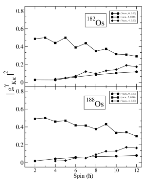
Figure 33: (Color online). Probabilities (18) of the vacuum components of the $\gamma$-band in ^182,188Os after diagonalization within the truncated space of the states projected from the quasi particle vacuum only (the vacuum only cases in figures and tables).

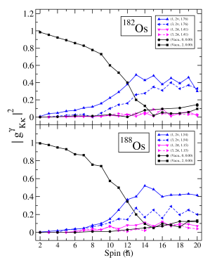
Figure 34: (Color online). Probabilities (18) of the pre-diagonalized high-j two-quasiparticle configurations in Fig. 30 for the $\gamma$-bands in ^182,188Os.

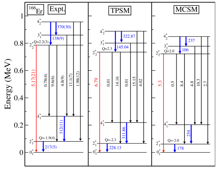
Figure 35: (Color online). Experimental energies, reduced transition probabilities $B(E2)$ (in W.u.) and static quadrupole moments $Q$ (in W.u.) of ¹⁶⁶Er NNDC compared with the MCSM Otsuka2019 and TPSM calculations.

Table 7: Energy characteristics of several models for ¹⁶⁶Er. The staggering parameter $S(3)$ is defined by Eq. (1). G. rot. lists the results for the Gamma-rotor as described in Sec. 2 (c.f. caption of Table 1). T. rot. lists the results for the triaixial rotor (Davydov) model AS60 with $\gamma=9^{\circ}$.

Model	${\left[\frac{E(2^{+}_{2})}{E(2^{+}_{1})}\right]}$	${\left[\frac{E(2^{+}_{2})}{E(4^{+}_{1})}\right]}$	${\left[\frac{E(4^{+}_{3})}{E(2^{+}_{2})}\right]}$	$S(3)$
Exp	9.7	3.0	2.5	-0.14
MCSM	11.8	3.6	2.8	-0.11
TPSM	11.1	3.4	3.1	-0.16
G. rot.	11.1	3.9	2.2	-0.17
T. rot	21.8	6.5	4.0	-0.16

4.8 Comparison with Monte Carlo Shell Model

The authors of Ref. Otsuka2019 ; Tsunoda2021 carried out large-scale Monte Carlo Shell Model (MCSM) calculations for ¹⁶⁶Er, which is considered to be a well deformed axially symmetric nucleus. For the lowest states of the ground- and $\gamma$-band, the experimental energies and the $B(E2)$ values for transitions between them are very well reproduced.

The MCSM states are represented by an ensemble of stochastically deformed Slater determinants, which are projected on to good angular momentum. Each of these states has definite intrinsic quadrupole moments $\langle Q_{0}\rangle$ and $\langle Q_{2}\rangle$, where the expectation value is taken with the deformed Slater determinant. Multiplying with the probability, each of these states appears in the total wave function, the so called T-plot is generated, which represents the probability distribution of the intrinsic quadrupole moments. For the $0^{+}_{1}$ ground state and the $2^{+}_{2}$ single-$\gamma$-band head, the T-plots show distributions that are centered at a triaxiality parameter of $\gamma=9^{\circ}$ with an approximate width of $15^{\circ}$. The same holds for the $4^{+}_{3}$ double $\gamma$ band head Otsuka2023 ; Otsuka2023pc .

The authors of Refs. Sun2000 ; Boutachkov2002 first applied the TPSM approach to the $\gamma$-bands in well deformed axial nuclei. The nucleus ¹⁶⁶Er belongs to this group. Table 7 and Fig. 35 compare our TPSM calculations with the MCSM results and the experiment. It is evident that the TPSM describes the energies and $B(E2)$ values as well as the MCSM. Thus, it corresponds to the MCSM picture of a $\gamma$-soft with slight triaxiality and it does not conflict with the TPSM input. As pointed out in the context of Eqs. (22), the triaxiality parameter $\gamma_{N}=21^{\circ}$ of the Nilsson potential corresponds to the substantial smaller estimate of $\gamma=13^{\circ}$ for the triaxiality of the charge and density distributions. The value being not far from the MCSM one and is consistent with the similarity of the TPSM and MCSM values for the observables in Fig. 35. In a forthcoming paper we will present the deformation parameters derived from the TPSM results by means of quadrupole shape invariants KM70 for several nuclides.

The similarity between the TPSM and MCSM does not come as a surprise. The MCSM states are comprised of stochastical configurations of the nucleons in a deformed mean-field, which are projected on to good angular momentum. The TPSM states are comprised of angular momentum projected quasi-nucleon configurations in a deformed mean-field. In the case of the MCSM, the diagonalization procedure picks out the favorite configurations that correspond to the appropriate deformation. In the case of the TPSM, the deformed mean-field is optimized from the outset, and the diagonalization within the space of quasiparticle configurations gets the right states.

The authors of Ref. Tsunoda2021 demonstrated that the phenomenological Gamma-rotor Hamiltonian discussed in Sec. 2 with a square well potential and a deep attraction for $4^{\circ}\leq\gamma\leq 14^{\circ}$ provides probability distributions $P(\gamma)$ that are similar to the ones from the T-Plots, and that the energies and $B(E2)$ values are nearly the same as for the rigid triaxial rotor (Dawydov limit) with $\gamma=9^{\circ}$ (see Fig. 1 and 2 of Ref. Tsunoda2021 ). The $B(E2$ values correlate well with the MCSM and the experiment. However, as seen in the line "T. rot." of Table 7 all three energy ratios of the rigid triaxial rotor are by factor 1.5-2 larger than the MCSM and experimental ratios.

The line "G. rot." in Table 7 lists the energy characteristics of the phenomenological Gamma-rotor of Sec. 2, with the parameters $\chi=100,~{}\xi=56$. This potential looks similar to the $\chi=50,~{}\xi=30$ case in Fig. 1, except that its minimum is located at $\gamma_{m}=9^{\circ}$ and that it is somewhat stiffer. The negative staggering parameter, $S(3)$, which indicate a certain amount of static triaxiality, is consistent with the MCSM values. The three energy ratios are similar to the ones of the MCSM as well. However, the ratios $\frac{B(E2,2^{+}_{2}\rightarrow 0^{+}_{1})}{B(E2,2^{+}_{1}\rightarrow 0^{+}_{1})}$=0.068, $\frac{B(E2,4^{+}_{3}\rightarrow 2^{+}_{2})}{B(E2,2^{+}_{2}\rightarrow 0^{+}_{1})}$=2.35, $\frac{B(E2,2^{+}_{2}\rightarrow 2^{+}_{1})}{B(E2,2^{+}_{1}\rightarrow 0^{+}_{1})}$=0.150 deviate from the respective MCSM ratios of 0.030, 1.89, 0.047.

For the states $0^{+}_{1},~{}2^{+}_{2}$ and $4^{+}_{3}$ of the 100-56 Gamma-rotor, we find that the width of the $\gamma$-probability distribution, defined as the distance of the classical turning point $E=V(\Delta\gamma)$ from 0, (see Sec. 2 and Appendix) changes as $\Delta\gamma=24^{\circ},~{}30^{\circ},~{}36^{\circ}$, respectively. The respective density distributions $P(\gamma)$ have well defined maxima at $\gamma=12^{\circ},~{}18^{\circ}$ and $24^{\circ}$. This is at variance with the T-plots of the TPSM, which look very similar for the three states

Hence, the MCSM quadrupole moments indicate a distribution of triaxial shapes that is about the same for the states $0^{+}_{1},~{}2^{+}_{2}$ and $4^{+}_{3}$ . However, the energy ratios of such an effective triaxial rotor deviate from the MCSM ratios. The MCSM energy ratios are approximately accounted for by an intrinsic shape distributions, the triaxiality of which increases with $I$ for the states $0^{+}_{1},~{}2^{+}_{2}$ and $4^{+}_{3}$. The increase leads to deviations of the $B(E2)$ ratios from the MCSM ones. Apparently, the results for both the energies and quadrupole moments from the microscopic MCSM and TPSM calculations cannot be accounted for by the same phenomenological Hamiltonian of the Gamma-rotor type.

5 Summary and Conclusions

The present work is a sequel to our earlier investigation of energy staggering of the $\gamma$-bands and its relation to nuclear triaxiality in the framework of the triaxial projected shell model (TPSM) approach GH14 ; SJ21 . We have undertaken a comprehensive investigation of both the energies and $B(E2)$ transition probabilities for a large set of thirty nuclides. We addressed the questions: (1) which are the observables that characterize the nature of the triaxiality, and (2) how the microscopic TPSM results can be interpreted in terms of the widely used phenomenology of the collective Bohr Hamiltonian?

The classification of atomic nuclei as “spherical, axial, triaxial, rigid, soft” is based on the collective Bohr Hamiltonian for the quadrupole degrees of freedom of the nuclear shape. To be specific, we discussed its simplified version, the Gamma-rotor, which assumes a fixed deformation $\beta$ and employs two parameters to describe the $\gamma$-dependence of the potential. In this generic model, the location $\gamma_{m}$ of the potential minimum defines the triaxiality and the distance $\Delta\gamma$ between the semiclassical turning points of the ground-state gives rise to the softness of the mode. We investigated how the energies of the lowest rotational bands and reduced $B(E2)$ probabilities within and among them depend on the triaxiality and softness.

The staggering phase of the energies of the $\gamma$-band built on the $2^{+}_{2}$ state has been widely used in the literature to distinguish between "$\gamma$-soft” and “$\gamma$-rigid" motion, with even-$I$-states lower for the former case, and even-$I$-states higher for the latter case. We demonstrated that this criterion is insufficient. To characterize the mode uniquely, it should be complemented by: the amplitude of the staggering parameter, $S(I)$, the ratios $E(2^{+}_{2})/E(2^{+}_{1}),~{}E(2^{+}_{2})/E(4^{+}_{1})$, the transition probabilities $B(E2,2^{+}_{2}\rightarrow 0^{+}_{1}),~{}B(E2,4^{+}_{3}\rightarrow 2^{+}_{2}),~{}B(E2,2^{+}_{3}\rightarrow 2^{+}_{1}),~{}B(E2,0^{+}_{2}\rightarrow 2^{+}_{2})$, and the static quadrupole moments $Q(2^{+}_{1}),~{}Q(2^{+}_{2})$.

The new observation of the present study is that the in-$\gamma$-band transition probabilities $B(E2,I\rightarrow I-2)$, stagger with a phase that is opposite to the phase of the energies. The appearance of these staggering patterns could be explained in terms of the interaction of the harmonic single $\gamma$-band with the harmonic ground-band and the harmonic double $\gamma\gamma 0$-band, which is the band based on the $0^{+}_{2}$ state. It represents two-phonons with opposite projection on the symmetry axis and, classically, a pulsation between prolate and oblate shape. The deviations of the potential from the quadratic form cause couplings between the bands. This band mixing interpretation connects the phenomenology and the microscopic TPSM results.

We have calculated the staggering of the $\gamma$-bands in the thirty nuclei and disregarding the quasiparticle admixtures, the staggering pattern of the $\gamma$-band is the same as for the triaxial nuclei according to phenomenology. The energies are always odd-$I$-down and for the intra-band, $B(E2,I\rightarrow I-2)$ values are even-$I$-down. This is expected because the TPSM uses a static triaxial deformation. The coupling between the $K=0$ and $K=2$ bands projected from the quasiparticle vacuum causes an upward shift of the even-$I$ members of the $\gamma$-band and is in complete analogy to the Bohr Hamiltonian. However, the staggering amplitude is much smaller than for the collective Hamiltonian with the same position of the $\gamma$-band relative to the ground-band.

In the context of the collective Bohr Hamiltonian, the reversal of the energy staggering to the even-$I$-down pattern of $\gamma$-softness reflects the coupling of the $\gamma$-band with the $\gamma\gamma 0$ pulsating mode, which incorporates the fluctuations of the $\gamma$-degree of freedom. In the TPSM context, it is the coupling to the set of two- and four- quasiparticle states, which modifies the vacuum pattern. The inclusion of the quasiparticle states into the TPSM vacuum configuration space reverses the phase of $S(I)$ for all selected nuclei, except for the six nuclei of ⁷⁶Ge, ¹¹²Ru, ^188,192Os, ¹⁹²Pt and ²³²Th. It is remarkable that TPSM reproduces the $(N-Z)$ dependence of the soft-rigid characteristic of $S(I)$ in all cases.

In the cases of ⁷⁶Ge SJ21 , ^104,112Ru Na23 ; SPRTBP and ^188,192Os, for which we studied the micro composition, it turned out that the coupling to the bands projected from the two-quasiparticle configurations of the high-j orbitals $f_{7/2}$, $g_{9/2}$, $h_{11/2}$ and $i_{13/2}$ dictates the staggering patterns of the $\gamma$-band energies and intra-band $B(E2,I\rightarrow I-2)$ values. We could not identify a simple intuitive mechanism yet, rather the interference between several terms seems to determine the final result. Nevertheless, we found a correlation for the Ru- and Os- isotopes. For nuclei with a sharp back-bend in the yrast sequence the energy staggering of the $\gamma$-band shows the even-$I$-down pattern of $\gamma$-softness and for nuclei with a smooth up-bend in the yrast sequence, the energy staggering of the $\gamma$-band shows the odd-$I$-down pattern of $\gamma$-rigidness.

Combining the present study with our previous work SJ21 ; Na23 ; SPRTBP , it can be concluded that TPSM approach describes the experimental energies and the available reduced $B(E2)$ transition probabilities of the yrast- and $\gamma$-bands in the selected thirty nuclei quite well. The same holds for the static quadrupole moments and g-factors of the $2^{+}_{1}$ states. The inter- and intra-band $B(E2)$ values were calculated in a systematic way and have been listed for future experimental comparisons. In order to elucidate the nature of the collective $\gamma$-mode in a more complete manner, the experimental transition probabilities connecting the states of the $\gamma$-band with bands built on excited $0^{+}_{n}$ and $4^{+}_{n}$ states are essential. This was demonstrated in our TPSM analysis of the rich COULEX data for the $\gamma$-soft triaxial nucleus ¹⁰⁴Ru Na23 .

It may be argued that the coupling to two- and four- quasiparticle excitations is a shell model representation of the fragmented $\gamma\gamma 0$-mode of the collective model. However, this interpretation needs to be substantiated by further analysis. The present work found that for the transitional nuclei ^154,156Gd , ^188,190,192Os and ¹⁹⁴Pt, the experimental $B(E2)$ values for the transitions from the rotational band on the $0^{+}_{2}$ state to the yrast and $\gamma$-bands are collectively enhanced. TPSM values are enhanced as well, however, the values noticeably deviate from experiment. The $0^{+}_{2}$ states in these nuclei are associated with the substantial changes in the $\beta$ deformation. It seems that the TPSM quasiparticle configuration space is too restrictive to quantitatively accommodate such changes. Improvement of the results can be achieved with the development of generator coordinate method (GCM) by considering TPSM wavefunctions as the generating states and $\beta$ and $\gamma$ as generator coordinates. This extension is presently being pursued along the lines of Refs. Chen2016 ; Chen2017 .

The present work can be considered as a part of the more general challenge in nuclear physics on how to associate the results from a large-scale matrix diagonalization with the intuitive collective model. The authors of Refs. Otsuka2019 ; Tsunoda2021 introduced the T-plots for relating their MCSM calculations to the collective shape dynamics. It was noted that ¹⁶⁶Er, traditionally classified as well deformed axial, has a T-plot that indicates a triaxial distribution around $\gamma=9^{\circ}$. We compared the MCSM energies and the $B(E2)$ values for the lowest states of the ground- and $\gamma$- bands with the one’s from the TPSM, and found that they agree rather well. This seems to indicate that the TPSM and MCSM results corresponds to a similar shape distribution.

In the present work, we followed the standard route of calculating energies and transition probabilities for the individual states and comparing them with the corresponding experimental values. Other approaches, for instance, the quadrupole shape invariant analysis will provide a complementry perspective on the relation between the TPSM and the collective model as we demonstrated for ¹⁰⁴Ru Na23 . We are in the process of performing a systematic shape invariant analysis for a set of nuclei discussed in this manuscript for which the Coulomb excitation data is available, and the results will be presented in a forthcoming publication.

Appendix: Detailed discussion of the Gamma-rotor model

Section 2 presented the results of the Gamma-rotor model for a selection collective potentials, which were used to classify the nature of the triaxiality of the nuclear shape. A summary of characteristic relations between energies and transition probabilities between of the lowest collective excitations of the quadrupole type was given. Here we provide the details of how these characteristic come about.

The potential $\chi-\kappa=200-0$ represents a rigid prolate nucleus with a harmonic $\gamma$-vibration far above the $4^{+}_{1}$ level of the ground-band and at about twice the energy are the two-phonon bands. The $K=4$ band labeled by $4^{+}_{3}$ in Fig. 1 represents a traveling wave generated by adding a second $K=2$ on top of the first with the same angular momentum along the symmetry axis. Transforming the ratio $B(E2,4^{+}_{3}\rightarrow 2^{+}_{2})/B(E2,2^{+}_{2}\rightarrow 0^{+}_{1})=0.094/0.033$ in Table 2 into the ratio of the matrix elements for transitions between states in an axial symmetric potential (see BM75 ; RW10 ), one obtains 1.42, which is approximately the ratio expected for the two- and one-phonon states of a harmonic vibration. The $K=0$ two-phonon state is generated by putting the second phonon with opposite angular momentum on top of the first, which represents a pulsating wave. Transforming the ratio $B(E2,0^{+}_{2}\rightarrow 2^{+}_{2})/B(E2,2^{+}_{2}\rightarrow 0^{+}_{1})=0.195/0.033$ in Table 2 into the ratio of the matrix elements for transitions between the states, one obtains 1.08, which is close to 1 expected for a harmonic vibration. The potential $\chi(1-\cos{3\gamma})=3/2\gamma^{2}+...$ is not exactly harmonic. The distances between the bands are large, such that the couplings of the harmonic bands with higher terms is small, which is reflected by the small value of $\bar{S}(6)=-0.03$ in Table 1.

The difference of the harmonic ratios can be understood by the following classical consideration. The $K=2$ one-phonon state correspond to a traveling wave in the plane perpendicular to the symmetry axis with $x=A\cos{\omega t}$ and $y=A\sin{\omega t}$. The average radiation power is $\propto\overline{x^{2}}+\overline{y^{2}}+2\overline{xy}=A^{2}$. The $K=4$ two-phonon state correspond to a traveling wave with the amplitude $\sqrt{2}A$. The radiation power of the $K=4$ two-phonon state is 2$A^{2}$. The $K=0$ two-phonon state correspond to a pulsating wave $x=\sqrt{2}A\cos{\omega t}$, which gives a radiation power $\propto\overline{x^{2}}=A^{2}$, corresponding to a ratio of 1.

The second limiting case is the $\gamma$-independent potential (0-0) of the Wilet-Jean model Wilets , which is discussed in detail in the textbook by Rowe and Wood RW10 (p. 117, 222 ff.) The states carry the seniority quantum number $v$. The quadrupole operator changes the seniority by 1, which is reflected by the $B(E2)$ values in Table 2. The static quadrupole moments vanish because they are matrix elements between states with the same $v$, and the $B(E2,2^{+}_{2}\rightarrow 0^{+}_{1})=B(E2,4^{+}_{3}\rightarrow 2^{+}_{2})=0$ because $v$ changes by 2. The states organize into $\Delta I=2$ bands of good signature, which are connected by strong $B(E2,I\rightarrow I-2)$ values (cf. also Fig. 2.3 of Ref. RW10 ). The band based on the $2^{+}_{2}$ state has $v=2+I/2$ and the one on $3^{+}_{1}$ has $v=3+I/2$. As the energy of the states is $E(v)=v(v+3)$, the two $\gamma$-band branches have a pronounced even-$I$-down staggering

$$S(I)=\frac{1}{8}\mp\left(\frac{I}{4}+\frac{9}{8}\right),~{}~{}I=\begin{array}[]{c}even\\ odd\end{array}.$$ (24)

The $\gamma$-band head has the same energy as the $4^{+}_{1}$ state of the ground-band, $E(2^{+}_{2})=E(4^{+}_{1})$, which is another signature of the $\gamma$-independent potential.

The shallow potential (10-0) and the soft potentials 20-0 and 50-0 illustrate the transition to rigid prolate limit (for more details see Ref. caprio11 ). The static quadrupole moments quickly approach the limit for prolate shape as a consequence of the seniority mixing. The $B(E2,2^{+}_{2}\rightarrow 0^{+}_{1})$ and $B(E2,4^{+}_{3}\rightarrow 2^{+}_{2})$ first increase because of the seniority mixing, and then they decrease because the amplitude of the $\gamma$-vibration decreases with $\chi$. The $B(E2,2^{+}_{2}\rightarrow 2^{+}_{1})$ values decrease due to the seniority mixing. The potential term $\cos 3\gamma$ couples states of $v=\pm 1$ RW10 . The coupling of the even-$I$ branch of the $\gamma$-band with the ground-band pushes them up. The even-$I$ band on top of the $0^{+}_{2}$ band does not couple because $v$ differs by 2, which reduces the staggering. For large values of the $\chi$ the higher order $\Delta v=\pm 1$ couplings quench the staggering. The repulsion caused by the coupling pushes the $2^{+}_{2}$ band head above the $4^{+}_{1}$ state of the ground-band.

The prolate harmonic limit provides another perspective that is instructive for interpreting the TPSM results. First inspect the probability density $P(\gamma)$ of the wave functions of the lowest bands obtained by integration over the angle degrees of freedom. Fig. 9 of Ref. caprio11 shows the case of potential 50-0. The density $P(\gamma)$ of the ground band is centered at $\gamma=0^{\circ}$ (after dividing out the volume element $\sin 3\gamma$). For the $\gamma$-band built on the $2^{+}_{2}$, the density has a maximum around 20^∘, which indicates that the state represents a wave that travels around the symmetry axis. The double $\gamma$-band ($\gamma\gamma 4$) built on the $4^{+}_{3}$ state has a maximum at $27^{\circ}$, which correspond to a traveling wave with a larger amplitude. (The concept of traveling (tidal) waves has been developed to microscopically calculate unharmonic many phonon excitation (see e.g. Ref. Frauendorf15 ).) For the double $\gamma$-band ($\gamma\gamma 0$) built on the 0${}^{+}_{2}$ state the density $P(\gamma)$ has two maxima with a zero at $15^{\circ}$ in between. The $0^{+}_{2}$ state represents a vibration of the triaxial shape between the prolate and oblate turning points (see BM75 ). The structure of the wave functions for other $\chi$ values is qualitatively the same. For larger $\chi$ the distributions $P(\gamma)$ are squeezed such that they fit into the potential (see 200-0 in Fig. 9 of caprio11 ). For smaller $\chi$ the distributions are shifted to larger $\gamma$ until they become symmetric about $30^{\circ}$ for $\chi=0$.

The deviation of “$1-\cos 3\gamma$” from the leading order term $3\gamma^{2}/2$ couples the even-$I$-states of the $\gamma$-band with the states of the ground-band and of the $0^{+}_{2}$ band, which, respectively, shifts them up or down. The down shift by the repulsion from the upper level prevails because it has a larger coupling matrix element. The reason is that the difference $|1-\cos 3\gamma-3\gamma^{2}/2|$ becomes larger with increasing $\gamma$, and the probability density $P(\gamma)$ of the ground-band is closer to zero localized than the one of the $0^{+}_{2}$ band, which has a zero and reaches further out (compare the cases g, $\gamma$ and $\gamma\gamma 0$) for the potential 200-0 in Fig. 9 of caprio11 ). With decreasing $\chi$, the potentials become shallower, which reduces distance between the bands. The level shift become larger because the energy differences decrease and the coupling matrix elements increase. The even-$I$-down staggering pattern of the $\gamma$-band evolves.

The potentials with $\chi$=0 represent the cases of maximal triaxiality. The term $\cos^{2}3\gamma$ of the potential is symmetric with respect to $\gamma\rightarrow 60^{\circ}\gamma$. It changes the seniority by $\Delta v=0,\pm 2$. The states have good $\gamma$-parity, which is reflected by $Q(2^{+}_{1})=Q(2^{+}_{2})=0$, $B(E2,2^{+}_{2}\rightarrow 0^{+}_{1})=0$ and $B(E2,4^{+}_{3}\rightarrow 2^{+}_{2})=0$ in Table 2. For small $\kappa$ the diagonal term $\langle Iv|\cos^{2}3\gamma|Iv\rangle$ dominates, which is larger for even $I$ ($\gamma$ parity even) than for odd $I$ ($\gamma$-parity odd). With increasing $\kappa$ level shifts decrease the even-$I$-down staggering of the $\gamma$-band until it disappears and changes into the even-$I$-up pattern (see 0-20 and 0-100 in Fig. 2 and Table 2). In the case of $\kappa<0$ with a barrier at $\gamma=30^{\circ}$ the shifts increase the staggering (see 0- (-20) in Fig. 2 and Table 2). With increasing $\kappa$ the $\Delta v=\pm 2$ terms become important and the structure of the bands based on the $0^{+}_{1},~{}2^{+}_{2},~{}4^{+}_{3}$ state quickly approach the ones of the triaxial rotor with $\gamma=30^{\circ}$.

The case is discussed as the Meyer-ter-Vehn limit in Ref. RW10 and is known as the symmetric top in molecular physics. The ratios of the moments of inertia are 4:1:1 for the medium, short, long axes, respectively, which means the eigenfunctions are the ones of a symmetric rotor, where $K$ is the angular momentum projection on the medium axis with the largest moment of inertia. The energy ratios are

$$\frac{E(I,K)}{E(2^{+}_{1})}=\frac{4I(I+1)-3K^{2}}{12}.$$ (25)

The corresponding ratio $E(2^{+}_{2})/E(4^{+}_{1})=0.75$ represent the limit of maximal triaxiality. For the potential 0-200 the ratio is 0.81 and for the potential 0-20 it is 0.97. The Meyer-ter-Vehn limit of the staggering parameter is

$$S(I)=\frac{1}{6}\pm\left(I-\frac{5}{2}\right),~{}~{}I=\begin{array}[]{c}even\\ odd\end{array}.$$ (26)

The value $\bar{S}(6)=4$ is to be compared with 3.87 for the potential 0-200 in Table 2. The quadruple operator is $(Q_{2}+Q_{-2})/\sqrt{2}$ with respect to the quantization axis “m”. The ratios of reduced transition probabilities are given by the corresponding ratios of the squares of the Clebsch-Gordan coefficients, (quoted e.g., Fig. 2.6 of Ref. RW10 ). For the lowest transitions, the $B(E2)$ values divided by the $B(E2,2^{+}_{1}\rightarrow 0^{+}_{1})$ are $B(E2,2^{+}_{2}\rightarrow 2^{+}_{1})$=1.43 (1.42, 1.42), $B(E2,4^{+}_{2}\rightarrow 2^{+}_{2})$=0.60 (0.58, 0.73), $B(E2,4^{+}_{1}\rightarrow 2^{+}_{1})$=1.39 (1.43, 1.42), $B(E2,3^{+}_{1}\rightarrow 2^{+}_{2})$=1.79 (1.71, 1.45), $B(E2,4^{+}_{3}\rightarrow 3^{+}_{1})$=0.56 (0.60, 0.86), where the ratios for the potentials 0-200 and 0-20 are quoted in parenthesis. The $B(E2)$ ratios for the Meyer-ter-Vehn limit are more rapidly approached than for the energies.

The transition from the symmetric triaxial to the prolate potentials involves the competition between the two potential terms discussed. Consider the soft potentials 0-50, 50-50 and 50-0. The symmetry with respect to $\gamma\rightarrow 60^{\circ}-\gamma$ of 0-50 is progressively broken in 50-50 and 50-0. As a consequence, the $B(E2,2^{+}_{2}\rightarrow 0^{+}_{1})$ and $B(E2,4^{+}_{3}\rightarrow 2^{+}_{2})$ become quickly large and the $B(E2,2^{+}_{2}\rightarrow 2^{+}_{1})$ decrease. The even-$I$-up staggering of the $\gamma$-band is reduced, and it reverses to the even-$I$-down pattern for the potentials. Along the sequence the state $2^{+}_{2}$ moves away from the state $4^{+}_{1}$ to larger energies. Both trends can be taken as signatures of decreasing triaxiality. The other cases between the prolate and symmetric triaxial limits exemplify the changes. Hence, a small staggering parameter indicates either prolate potential or a transitional one, where the former has a large and the latter a small ratio $E(2^{+}_{2})/E(4^{+}_{1})$. For all the cases, the $0^{+}_{2}$ states represent a pulsating $\gamma$ vibration with a zero in the $P(\gamma)$ probability density, the position of which depends on the potential parameters (see Fig. 9 of caprio11 ). The $B(E2,0^{+}_{2}\rightarrow 2^{+}_{2})$ values are always substantial, being larger for more flatter potentials.

The reversal of the phase of $S(I)$ with increasing $\kappa$ is understood as follows: The term symmetric $(\cos 3\gamma)^{2}$ couples the $\gamma$-band strongly to the ground-band because both the states do not have a zero in the $\gamma$ degree of freedom. The coupling to the $0^{+}_{2}$ band is weaker because its states have a zero in the $\gamma$ degree of freedom. Hence the repulsion between the even-$I$-states of the ground- and $\gamma$-band prevails which generates even-$I$-up staggering pattern. As discussed above, the “$\cos 3\gamma$” term generates the even-$I$-down staggering pattern, and the competition of both terms determine the phase of $S(I)$.

The potential 20-50 represents a case incipient of prolate-oblate shape coexistence. There is a regular rotational ground-band with $P(\gamma)$ localized on the prolate side. The $0^{+}_{2}$ state comes low in energy. The second bump of $P(\gamma)$ on the oblate side is larger than the first on the prolate side. The $\Delta I=2$ sequence built on the $0^{+}_{2}$ state can be interpreted as the "oblate" rotational band. However, one can alternatively interpret the sequence as a band built on a large-amplitude $\gamma$-vibration, which applies to all potentials (see discussion of the WJ limit related to Fig. 4.15 of Ref. RW10 ).

Now the mixing of the even-$I$ members of the harmonic ground-band (g), $\gamma$-band ($\gamma$) and double-$\gamma$-band ($\gamma\gamma 0$) is considered in detail,

$$\psi(I,M,\Omega,\gamma)=c_{g}\psi_{g}(I,M,\Omega,\gamma)$$

$$+c_{\gamma\gamma 0}\psi_{\gamma\gamma 0}(I,M,\Omega,\gamma)$$

$$+\sqrt{1-c_{g}^{2}-c_{\gamma\gamma 0}^{2}}\psi_{\gamma}(I,M,\Omega,\gamma),$$ (27)

where $c_{g}$ and $c_{\gamma\gamma 0}$ are the mixing amplitudes. The basis states are eigenfunctions of the Gamma-rotor Hamiltonian (3) with the harmonic prolate potential $\chi 3/2\gamma^{2}$,

$$\psi_{g}(I,M,\Omega,\gamma)=N(I)D^{I}_{M0}(\Omega)\phi_{g}(\gamma),$$ (28)

$$\psi_{\gamma}(I,M,\Omega,\gamma)=N(I)D^{I}_{M2}(\Omega)\phi_{\gamma}(\gamma),$$ (29)

$$\psi_{\gamma\gamma 0}(I,M,\Omega,\gamma)=N(I)D^{I}_{M0}(\Omega)\phi_{\gamma\gamma 0}(\gamma),$$ (30)

where $N(I)$ are the normalization factors of the $D$ functions. The $\psi(\gamma)$ are the normalized wave functions in the $\gamma$-degree of freedom, the probability distributions are shown in Fig. of Ref. caprio11 . Their phases are chosen such that they are positive for small $\gamma$. The reduced transition matrix elements for the $I\rightarrow I-2$ transitions in units of $3ZR_{0}^{2}\beta/4\pi$ are the following (cf. Ref. BM75 Eq. (4-91)).

$$\langle I-2,\gamma||{\cal M}(E2)||I,\gamma\rangle=$$

$$\sqrt{2I+1}\langle I~{}2~{}2~{}0|I-2~{}2\rangle\langle\psi_{\gamma}|\cos\gamma|\psi_{\gamma}\rangle~{}>0.$$ (31)

$$\langle I-2,g||{\cal M}(E2)||I,\gamma\rangle=$$

$$\sqrt{2I+1}\langle I~{}2~{}2~{}-2|I-2~{}0\rangle\langle\psi_{g}|\sin\gamma|\psi_{\gamma}\rangle/\sqrt{2}~{}>0.$$ (32)

The matrix element is positive because both $\psi_{g}(\gamma)$ and $\psi_{\gamma}(\gamma)$ do have a zero and are positive over the whole $\gamma$ range.

$$\langle I-2,\gamma\gamma 0||{\cal M}(E2)||I,\gamma\rangle=$$

$$\sqrt{2I+1}\langle I~{}2~{}2~{}-2|I-2~{}0\rangle\langle\psi_{\gamma\gamma 0}|\sin\gamma|\psi_{\gamma}\rangle/\sqrt{2}~{}<0.$$ (33)

The function $\psi_{\gamma\gamma 0}(\gamma)$ is positive for small $\gamma$ and negative for large $\gamma$, while $\psi_{g}(\gamma)$ is positive over the whole $\gamma$ range. Integrating the $\sin\gamma$ function results in a negative value because it weights more the large $\gamma$ values. As discussed for the prolate regime, $|\langle I-2,\gamma\gamma 0||{\cal M}(E2)||I,\gamma\rangle|=\langle I-2,g||{\cal M}(E2)||I,\gamma\rangle$ in the harmonic limit.

The coupling is generated by the difference of the potential from its prolate quadratic approximation

$$V_{c}(\gamma)=\chi(1-\cos 3\gamma)+\kappa(\cos^{2}3\gamma-1)-\chi\frac{3\gamma^{2}}{2}.$$ (34)

For a prolate potential ($\kappa=0$) $V_{c}(\gamma)$ is weakly negative for small $\gamma$ and strongly negative for large $\gamma$. The coupling matrix element $V_{g\gamma}=\langle\psi_{g}|V_{c}(\gamma)|\psi_{\gamma}\rangle<0$. The matrix element $V_{\gamma\gamma 0\gamma}=\langle\psi_{\gamma\gamma 0}|V_{c}(\gamma)|\psi_{\gamma}\rangle>0$ because $\psi_{\gamma\gamma 0}(\gamma)<0$ for large $\gamma$ where $|V_{c}|$ is large. For $\psi_{g}(\gamma)$ is predominantly localized in the small-$\gamma$ region and $\psi_{\gamma\gamma 0}(\gamma)$ is predominantly localized in the large-$\gamma$ region $|V_{g\gamma}|<V_{\gamma\gamma 0\gamma}$. With $E_{\gamma}(I)-E_{g}(I)=E_{\gamma\gamma 0}-E_{\gamma}(I)$ the diagonalization of the 3 x 3 matrix gives a down-shift of the middle eigenvalue, which represents the $\gamma$-band with admixtures. As expected, the repulsion from the $\gamma\gamma 0$ state prevails over the one from the g-state because of the larger coupling matrix element of the former. The mixing amplitudes are both negative, where $|c_{\gamma\gamma 0}|>|c_{g}|$, which increases the reduced matrix element by $|c_{\gamma\gamma 0}-c_{g}|\langle I-2,g||{\cal M}(E2)||I,\gamma\rangle$.

Now consider a triaxial potential by increasing $\kappa$ while keeping $\chi$ constant (see 50-0, 50-50, 50-100 in Fig. 1). The term $\kappa(\cos^{2}3\gamma-1)$, which decreases $V_{c}$, is symmetric about $30^{\circ}$. As a cosequence,the coupling matrix element $V_{g\gamma}=\langle\psi_{g}|V_{c}(\gamma)|\psi_{\gamma}\rangle$ becomes more and more negative. The matrix element $V_{\gamma\gamma 0\gamma}=\langle\psi_{\gamma\gamma 0}|V_{c}(\gamma)|\psi_{\gamma}\rangle$ does not change much because $\psi_{\gamma\gamma 0}(\gamma)$ is antisymmetric about $30^{\circ}$. Hence for a certain value of $\kappa$ coupling matrix element reverses order to $|V_{g\gamma}|>V_{\gamma\gamma 0\gamma}$ and the staggering of the energies and of the $B(E2)$ values change to the even-$I$-up pattern of triaxial potentials.

For the limiting case of the WJ potential the staggering of the inband $B(E2)$ values reflects the seniority conservation. The $B(E2)$ transition operator (5) has the selection rule $\Delta v=\pm 1$. As seen in Fig. 2, the transitions $I_{1}\rightarrow I_{1}-2,~{}I$-odd are allowed while the transitions $I_{2}\rightarrow I_{2}-2,~{}I$-even are forbidden. This results in a staggering pattern of $SE22(I)$ with the phase opposite to the one of $S(I)$. In analogous conjecture holds for $SBE21(I)$. For the symmetric top limit the reversed staggering pattern appears as a consequence of the fact that the ratios of $B(E2)$ values follow the Alaga rules.

References

- (1) A. Bohr, B.R. Mottelson, Nuclear Structure (W. A. Benjamin, New York, Amsterdam, 1975)
- (2) S. Frauendorf, International Journal of Modern Physics E 24, 1541001 (2015)
- (3) T. Otsuka, A. Gade, O. Sorlin, T. Suzuki, Y. Utsuno, Rev. Mod. Phys. 92, 015002 (2020)
- (4) B.A. Brown, Physics 4, 525 (2022)
- (5) A. Poves, E. Caurier, F. Nowacki, K. Sieja, Phys. Scripta 2012, 014030 (2012)
- (6) T. Otsuka, Y. Tsunoda, T. Abe, N. Shimizu, P. Van Duppen, Phys. Rev. Lett. 123, 222502 (2019)
- (7) Y. Tsunoda, T. Otsuka, Phys. Rev. C 103, L021303 (2021)
- (8) J.A. Sheikh, G.H. Bhat, W.A. Dar, S. Jehangir, P.A. Ganai, Phys. Scr. 91, 063015 (2016)
- (9) J.A. Sheikh, K. Hara, Phys. Rev. Lett. 82, 3968 (1999)
- (10) G.H. Bhat, W.A. Dar, J.A. Sheikh, Y. Sun, Phys. Rev. C 89, 014328 (2014)
- (11) J.A. Sheikh, G.H. Bhat, Y. Sun, G.B. Vakil, R. Palit, Phys. Rev. C 77, 034313 (2008)
- (12) C.L. Zhang, G.H. Bhat, W. Nazarewicz, J.A. Sheikh, Y. Shi, Phys. Rev. C 92, 034307 (2015)
- (13) J.A. Sheikh, G.H. Bhat, Y.X. Liu, F.Q. Chen, Y. Sun, Phys. Rev. C 84, 054314 (2011)
- (14) G.H. Bhat, J.A. Sheikh, R. Palit, Phys. Lett. B 707, 250 (2012)
- (15) G.H. Bhat, J.A. Sheikh, Y. Sun, U. Garg, Phys. Rev. C 86, 047307 (2012)
- (16) S. Jehangir, G.H. Bhat, J.A. Sheikh, S. Frauendorf, S.N.T. Majola, P.A. Ganai, J.F. Sharpey-Schafer, Phys. Rev. C 97, 014310 (2018)
- (17) P. Ring, P. Schuck, The Nuclear Many-Body Problem (Springer Berlin Heidelberg, 1980)
- (18) S. Jehangir, G.H. Bhat, J.A. Sheikh, S. Frauendorf, W. Li, R. Palit, N. Rather, Eur. Phys. J. A 57, 308 (2021)
- (19) N. Zamfir, R. Casten, Physics Letters B 260, 265 (1991)
- (20) E.A. McCutchan, D. Bonatsos, N.V. Zamfir, R.F. Casten, Phys. Rev. C 76, 024306 (2007)
- (21) A.S. Davydov, in Proc.Intern.Conf. on Nuclear Structure (Kingston, Canada), eds. D. A. Bromley and E. W. Vogt (University of Toronto Press, Toronto, 1960) p. 801 (1970)
- (22) K. Kumar, Phys. Rev. C 1, 369 (1970)
- (23) C. Baktash, J.X. Saladin, J.J. O’Brien, J.G. Alessi, Phys. Rev. C 18, 131 (1978)
- (24) C. Baktash, J.X. Saladin, J.J. O’Brien, J.G. Alessi, Phys. Rev. C 22, 2383 (1980)
- (25) A. Davydov, G. Filippov, Nuclear Physics 8, 237 (1958)
- (26) L. Wilets, M. Jean, Phys. Rev. 102, 788 (1956)
- (27) M.A. Caprio, Phys. Rev. C 83, 064309 (2011)
- (28) I. Stefanescu, A. Gelberg, J. Jolie, P. Van Isacker, P. von Brentano, Y. Luo, S. Zhu, J. Rasmussen, J. Hamilton, A. Ramayya et al., Nuclear Physics A 789, 125 (2007)
- (29) A. Bohr, Mat. Fys. Medd. K. Dan. Vidensk. Selsk. 26 (1952)
- (30) K. Kumar, M. Baranger, Nuclear Physics A 92, 608 (1967)
- (31) J. Eisenberg, W. Greiner, Nuclear Theory, 3rd ed. (North-Holland Amsterdam, 1987), ISBN 0-444-87073-3
- (32) Y. Sun, K. Hara, J.A. Sheikh, J.G. Hirsch, V. Velázquez, M. Guidry, Phys. Rev. C 61, 064323 (2000)
- (33) P. Boutachkov, A. Aprahamian, Y. Sun, J. Sheikh, S. Frauendorf, Eur. Phys. J. A 15, 455 (2002)
- (34) G. Gneuss, U. Mosel, W. Greiner, Physics Letters B 30, 397 (1969)
- (35) P.O. Hess, M. Seiwert, J. Maruhn, W. Greiner, Zeitschrift fur Physik A Hadrons and Nuclei 296, 147 (1980)
- (36) A. Faessler, W. Greiner, R.K. Sheline, Nuclear Physics 70, 33 (1965)
- (37) N. Nazir, S. Jehangir, S.P. Rouoof, G.H. Bhat, J.A. Sheikh, N. Rather, S. Frauendorf, Phys. Rev. C 107, L021303 (2023)
- (38) J. Srebrny, T. Czosnyka, C. Droste, S. Rohoziński, L. Próchniak, K. Zajac, K. Pomorski, D. Cline, C. Wu, A. Bäcklin et al., Nuclear Physics A 766, 25 (2006)
- (39) M.A. Caprio, Phys. Rev. C 83, 064309 (2011)
- (40) D. Rowe, J. Wood, Fundamentals of Nuclear Models: Foundational Models (World Scientific, 2010), ISBN 9789812569554
- (41) National Nuclear Data Center, Brookhaven National Laboratory, Upton, NY, USA. (https://www.nndc.bnl.gov)
- (42) M.A. Lee, Nucl. Data Sheets 31, 381 (1980)
- (43) H. Emling, E. Grosse, D. Schwalm, R. Simon, H. Wollersheim, D. Husar, D. Pelte, Physics Letters B 98, 169 (1981)
- (44) S.N.T. Majola, D.J. Hartley, L.L. Riedinger, J.F. Sharpey-Schafer, J.M. Allmond, C. Beausang, M.P. Carpenter, C.J. Chiara, N. Cooper, D. Curien et al., Phys. Rev. C 91, 034330 (2015)
- (45) B.M. Musangu, E.H. Wang, J.H. Hamilton, S. Jehangir, G.H. Bhat, J.A. Sheikh, S. Frauendorf, C.J. Zachary, J.M. Eldridge, A.V. Ramayya et al., Phys. Rev. C 104, 064318 (2021)
- (46) K. Hara, Y. Sun, International Journal of Modern Physics E 04, 637 (1995)
- (47) S.G. Nilsson, C.F. Tsang, A. Sobiczewski, Z. Szymański, S. Wycech, C. Gustafson, I.L. Lamm, P. Möller, B. Nilsson, Nucl. Phys. A 131, 1 (1969)
- (48) K. Hara, S. Iwasaki, Nuclear Physics A 332, 61 (1979)
- (49) K. Hara, S. Iwasaki, Nuclear Physics A 348, 200 (1980)
- (50) L.J. Wang, F.Q. Chen, Y. Sun, Phys. Lett. B 808, 135676 (2020)
- (51) R. Shimizu, T. Shoji, M. Matsuzaki, Phys. Rev. C 77, 024319 (2008)
- (52) S. Raman, C. Nestor, P. Tikkanen, Atomic Data and Nuclear Data Tables 78, 1 (2001)
- (53) B. Singh, D.A. Viggars, Nucl. Data Sheets 42, 233 (1984)
- (54) A.R. Farhan, B. Singh, Nucl. Data Sheets 110, 1917 (2009)
- (55) J. Blachot, Nuclear Data Sheets 108, 2035 (2007)
- (56) D. De Frenne, A. Negret, Nucl. Data Sheets 109, 943 (2008)
- (57) J. Blachot, Nuclear Data Sheets 91, 135 (2000)
- (58) G. Gurdal, F. Kondev, Nuclear Data Sheets 113, 1315 (2012)
- (59) S. Lalkovski, F. Kondev, Nuclear Data Sheets 124, 157 (2015)
- (60) C.W. Reich, Nucl. Data Sheets 110, 2257 (2009)
- (61) C. Reich, Nuclear Data Sheets 113, 2537 (2012)
- (62) N. Nica, Nucl. Data Sheets 141, 1 (2017)
- (63) N. Nica, Nucl. Data Sheets 176, 1 (2021)
- (64) C.W. Reich, Nucl. Data Sheets 108, 1807 (2007)
- (65) B. Singh, J. Chen, Nuclear Data Sheets 147, 1 (2001)
- (66) C.M. Baglin, Nuclear Data Sheets 109, 1103 (2008)
- (67) C.M. Baglin, E.A. McCutchan, S. Basunia, E. Browne, Nucl. Data Sheets 153, 1 (2018)
- (68) S.C. Wu, H. Niu, Nuclear Data Sheets 100, 483 (2003)
- (69) B. Singh, Nucl. Data Sheets 130, 21 (2015)
- (70) C.M. Baglin, Nucl. Data Sheets 111, 275 (2010)
- (71) C.M. Baglin, Nuclear Data Sheets 99, 1 (2003)
- (72) B. Singh, Nucl. Data Sheets 95, 387 (2002)
- (73) B. Singh, J. Chen, Nuclear Data Sheets 169, 1 (2020)
- (74) C.M. Baglin, Nuclear Data Sheets 113, 1871 (2012)
- (75) J. Chen, B. Singh, Nuclear Data Sheets 177, 1 (2021)
- (76) E. Browne, Nucl. Data Sheets 107, 2579 (2006)
- (77) F. Chukreev, V. Makarenko, M. Martin, Nuclear Data Sheets 97, 129–240 (2002)
- (78) S. Frauendorf, G. Bhat, N. Nazir, N. Rather, S. Rouoof, S. Jehangir, J. Sheikh, arXiv 2311.00190 (2023,)
- (79) S. Frauendorf, Phys. Rev. C 97, 069801 (2018)
- (80) S. Frauendorf, Rev. Mod. Phys. 73, 463 (2001)
- (81) S. Frauendorf, Physica Scripta 93, 043003 (2018)
- (82) Y. Toh, C.J. Chiara, E.A. McCutchan, W.B. Walters, R.V.F. Janssens, M.P. Carpenter, S. Zhu, R. Broda, B. Fornal, B.P. Kay et al., Phys. Rev. C 87, 041304 (2013)
- (83) P. Moller, A.J. Sierk, R. Bengtsson, H. Sagawa, T. Ichikawa, Phys. Rev. Lett. 103, 212501 (2009)
- (84) K.S. Krane, Phys. Rev. C 10, 1197 (1974)
- (85) K.C. Chung, A. Mittler, J.D. Brandenberger, M.T. McEllistrem, Phys. Rev. C 2, 139 (1970)
- (86) Z. Grabowski, S. Gustafsson, I. Marklund, I. Häller, Nuclear Physics 20, 159 (1960)
- (87) R.M. Lieder, J.E. Draper, Phys. Rev. C 2, 531 (1970)
- (88) J.M. Eldridge, B. Fenker, J.H. Hamilton, C. Goodin, C.J. Zachary, E. Wang, A.V. Ramayya, A.V. Daniel, G.M. Ter-Akopian, Y.T. Oganessian et al., European Physical Journal A 54, 15 (2018)
- (89) I. Uluer, C. Kalfas, W. Hamilton, R. Fox, D. Warner, M. Finger, D. Chung, Journal of Physics G: Nuclear Physics 1, 476 (1999)
- (90) T.I. Kracíková, M. Finger, M. Krmar, K. Kumar, A. Janata, N.A. Lebedev, V.N. Pavlov, E. Šimečková, Phys. Rev. C 58, 1986 (1998)
- (91) J. Domingos, G. Symons, A. Douglas, Nuclear Physics A 180, 600 (1972)
- (92) A.D. Ayangeakaa, R.V.F. Janssens, S. Zhu, D. Little, J. Henderson, C.Y. Wu, D.J. Hartley, M. Albers, K. Auranen, B. Bucher et al., Phys. Rev. Lett. 123, 102501 (2019)
- (93) C. Wu, D. Cline, T. Czosnyka, A. Backlin, C. Baktash, R. Diamond, G. Dracoulis, L. Hasselgren, H. Kluge, B. Kotlinski et al., Nuclear Physics A 607, 178 (1996)
- (94) J. Allmond, R. Zaballa, A.M. Oros-Peusquens, D. Kulp, J. Wood, Physical Review C - PHYS REV C 78, 014302 (2008)
- (95) B.P. McCormick, A.E. Stuchbery, B.A. Brown, G. Georgiev, B.J. Coombes, T.J. Gray, M.S.M. Gerathy, G.J. Lane, T. Kibédi, A.J. Mitchell et al., Phys. Rev. C 100, 044317 (2019)
- (96) A. Smith, D. Patel, G. Simpson, R. Wall, J. Smith, O. Onakanmi, I. Ahmad, J. Greene, M. Carpenter, T. Lauritsen et al., Physics Letters B 591, 55 (2004)
- (97) G. Menzen, A. Wolf, H. Lawin, G. Lhersonneau, K. Sistemich, Zeitschrift fur Physik A Hadrons and Nuclei 321, 593 (1985)
- (98) B.A. Bian, Y.M. Di, G. Long, Y.S. Sun, J.Y. Zhang, J. Sheikh, Phys. Rev. C 75, 014312 (2007)
- (99) T. Otsuka, Presentation at the 17the International Conference on Gamma Spectroscopy, Grenoble, 17-23 July (2023)
- (100) T. Otsuka, Private communication (2023)
- (101) F.Q. Chen, J.L. Egido, Phys. Rev. C 93, 064313 (2016)
- (102) F.Q. Chen, J.L. Egido, Phys. Rev. C 95, 024307 (2017)