Including individual Customer Lifetime Value and competing risks in tree-based lapse management strategies

Abstract

A retention strategy based on an enlightened lapse model is a powerful profitability lever for a life insurer. Some machine learning models are excellent at predicting lapse, but from the insurer’s perspective, predicting which policyholder is likely to lapse is not enough to design a retention strategy. In our paper, we define a lapse management framework with an appropriate validation metric based on Customer Lifetime Value and profitability.
We include the risk of death in the study through competing risks considerations in parametric and tree-based models and show that further individualization of the existing approaches leads to increased performance. We show that survival tree-based models outperform parametric approaches and that the actuarial literature can significantly benefit from them. Then, we compare, on real data, how this framework leads to increased predicted gains for a life insurer and discuss the benefits of our model in terms of commercial and strategic decision-making.
Key words: Machine Learning, Life insurance, Customer lifetime value, Lapse, Lapse management strategy, Competing risks, Tree-based models

1 Introduction

In life insurance, “lapse risk” or “persistency risk” is the risk that the policyholder will cancel the contract at a time other than when the issuer expected when pricing the contract ([40]). A life insurance policy can lapse if the policyholder stops paying the premiums required to keep the policy in force. This can happen if the policyholder becomes unable or unwilling to make the premium payments or if the policyholder chooses to surrender the policy for its cash value. When a policy lapses, the coverage and benefits the policy provides are no longer in effect, and the policyholder will not receive any payout if they pass away after the policy has lapsed. This risk is not considered an insurance risk because the payment to the policyholder “is not contingent on an uncertain future event that adversely affects the policyholder”. However, lapse management is still undoubtedly a primary concern for life insurers. Lapses may substantially affect a company’s solvency, its future profits and cash flows ([9; 10]) or its Asset and Liabilities Management (ALM) ([39; 23; 21; 20]). The importance of measuring lapse and churn behaviours is global; it goes from yielding individual estimations of the Customer Lifetime Values (CLV) to being an estimator of a firm’s profitability ([27; 26]) or strength ([2]). Therefore, this paper focuses on developing strategies to prevent lapses before they occur: for a life insurer, an enlightened and proactive lapse management strategy (LMS) is critical for successful monitoring and steering. This paper is about defining a framework for a life insurer to measure and optimise the future loss or profit to be expected when applying such an LMS.

Part of the literature on lapse management adopts an economic-centred point of view ([16; 41; 37; 15; 38; 57; 59; 60; 49; 53; 62]); we refer the reader to the complete bibliometric analysis on this topic by [58] for a summarised view of all these references. This economic-centred research aims to determine lapse factors like interest rates, gross domestic product, or unemployment rates. They are driven by economic hypotheses such as the emergency fund hypothesis (lapsing is a way of constituting an emergency fund), the policy replacement hypothesis (lapsing will occur when one changes its policy) or the interest rate hypothesis (lapsing depends strongly on rate change and arbitration).
On the other hand, a large part of the literature investigates the individual determinants of lapse with policyholder-centred approaches. Micro-oriented features such as policyholder’s personal information or the policy characteristics have shown to give valuable insights into lapse behavior ([55; 48; 20; 33]). [63] as well as [24]’s works indicate that policyholders’ features such as age and the number of beneficiaries are significant lapse factors, whereas [59] dismissed those results. A recent work from [45] proposes a comparison of lapse management strategies based on an innovative evaluation metric derived from the Customer Lifetime Value (CLV). [32] investigates the benefits of incorporating spatial analysis in lapse modeling, and [3] shows with an approach based on random forests that microeconomic features such as the company’s commercial approach for instance - is determining in the lapse decision. In contrast, macro-economical features only have a limited effect. This variety of results – sometimes contradicting each other – demonstrates the active interest in this research problem.

This paper focuses on lapse management strategy and retention targeting and will contribute to the existing literature on the relationship between retention strategy and lapse prediction: as in [2] and [45], our goal is not only to model the lapse behavior but rather to select policyholders that are expected to generate future profit, if targeted by a retention strategy. This work shows that a well-chosen strategy, based on individualized CLV and directed towards a well-chosen target, increases the insurer’s expected profitability. A critical concept that motivates many CLV-driven decisions is that customers should be judged as assets based on their future profitability for the insurer. Thus, since retention often serves as the basis for CLV models ([28; 18; 44] - sometimes specifically designed for targeting tasks ([61]) - and since CLV considerations should drive retention management, it seems natural to extend the existing life insurance applications linking those topics together. We make decision-making a central concern of our work and suggest proactive lapse management tools allowing the insurer to undertake actions to prevent the causes of lapse; that is opposed to a reactive management approach where decisions are taken after lapses and aim at recapturing lost policyholders.

The goal of this paper is to create an individualized CLV model that will be used to enhance classical binary churn models. We will then have a model for lapse management strategy and retention targeting that we further improve with tree-based survival analysis and competing risks considerations. The global framework is directly inspired by [45]. We try in this paper to build from that existing work and extend it. We model an individual future CLV with a new survival approach for which the risks of death and lapse are treated as mutually exclusive competing risks. For this purpose, we introduce parametric approaches - Cox cause-specific and subdistribution models - as well as tree-based survival models - Random Survival Forest (RSF) and Gradient boosting survival analysis. We focus here on tree-based models as they are often considered state-of-the-art models ([25]). Thus we introduce tree-based machine learning algorithms for binary prediction, including Classification and Regression Tree (CART), Random forests (RF), and Extreme Gradient Boosting (XGBoost) to lapse behavior modeling. CART and XGBoost ([48; 45]) were used in the literature for lapse modeling but have yet to be applied to predicting life insurance lapses in a competing risk setting. To our knowledge, while Random Survival Forest has been used for churn prediction recently ([56]), both RSF and Gradient boosting survival analysis have never been used for that purpose before in an actuarial context.
Our contribution to the actuarial literature is twofold. First, we detail a two-step lapse management modeling approach: we fit parametric and tree-based competing risk individual survival models to estimate individualized future CLVs that are part of an evaluation metric for tree-based lapse management models. Second, this work includes a business-oriented discussion of the results achieved by this framework, which is missing from existing similar approaches.
The results and discussions show that a CLV-based lapse management strategy very often outperforms a more classical binary classification approach, even with competing risks and individualized considerations. When the latter yields profitable retention gain, the former can produce higher profits, up to more than 60%. If a loss-inducing retention strategy is considered, our methodology limits the loss considerably, often setting 0 as a floor limit or even turning it into a profit-inducing retention strategy. Sensitivity analysis explores the influence of conjectural and structural parameters.

The rest of this paper is structured as follows. We briefly outline the data used in our study in Section 2. In Section 3, we then introduce the binary classification models we selected and detail our study’s methodology, describing the classical and CLV-based performance measures and discussing substantial parametrization improvements over existing approaches. Then, Section 4 details our two-step methodology, with the parametric and non-parametric modelings of individual survival predictions, in a competing risks framework and then their implementation in the tree-based classification approaches considered. Section 5 presents the real-life application we considered and the different results it produces. Those results are analyzed and discussed in Section 6 with commercial and strategical decision-making orientations. Eventually, Section 7 concludes this paper.

2 Data

We apply our framework to a real-world insurance portfolio. For privacy reasons, all the data, statistics, product names and perimeters presented in this paper have been either anonymized or modified. All analyses, discussions and conclusions remain unchanged.

We illustrate our methodology with a life insurance portfolio from a French insurer contracted between 1997 and 2018. Each record in the data set represents a unique policy for a unique policyholder. In the following sections, we will often refer to a unique pair of policy and policyholder by the term “subject”. The dataset contains 251,325 rows with 248,737 unique policies and 235,076 unique policyholders. It means that some policies are shared between several policyholders and that one individual can detain several insurance policies. The dataset contains 43 covariates described in Table 1.

Table 1: Data set description

Covariates (Numerical, Categorical, Date) Description ID CDI_ID_PERSONNE Policyholder (PH) unique ID CDI_ID_CONTRAT Policy unique ID PH-level information CDI_DT_NAISSANCE PH’s birth date (main PH when several policyholders owns one policy) Age_souscription PH’s age at subscription Nb_Contrats Number of different policies owned by the policyholder CDI_CD_SEXE PH’s gender (1=Female; 2=Male; other=Non precised) CDI_DESTINATAIRE_COURRIER Anonymised PH’s name CDI_NUM_ET_NOM_VOIE Anonymised PH’s address CDI_CD_POSTAL Anonymised PH’s postcode CDI_COMMUNE Anonymised PH’s city of residence CDI_TOP_ASSURE Binary: 1 if PH is the main PH on the policy, 0 otherwise Policy-level informations CDI_TYPE_PRODUIT Type of product (“Top-end product” or “Classical product”) CDI_NOM_PRODUIT Name of life insurance product (“Product 1”, “Product 2” or “Product 3”) CDI_PARTENAIRE Name of the insurance distributor CDI_DATE_DEB_CONTRAT Policy’s start date CDI_DATE_FIN_CONTRAT Policy’s end date START_YEAR Policy’s start year END_YEAR Policy’s end year SENIORITY Policy’s seniority (final seniority if the policy is ended, current seniority otherwise) STATE Policy’s state (“Active”, “Lapsed”, or “Death” if the policy ended following PH’s death) YEAR Last year of observation External data DISCOUNT RATE Discount rate corresponding to the last year of observation Policy’s cumulated financial flows TOTAL_PREMIUM_AMOUNT Total face amount of the policy TOTAL_EURO_PREMIUM_AMOUNT Face amount of the policy in euros TOTAL_UC_PREMIUM_AMOUNT Face amount of the policy in units of account ARBITRATION_EURO Cumulated arbitration amount of the policy in euros ARBITRATION_UC Cumulated arbitration amount of the policy in units of account FEES_EURO Cumulated fees amount of the policy in euros FEES_UC Cumulated fees amount of the policy in units of account OTHER_EURO Cumulated other parts of the face amount of the policy in euros OTHER_UC Cumulated other parts of the face amount of the policy in units of account PREMIUM_EURO Cumulated payments amount of the policy in euros PREMIUM_UC Cumulated payments amount of the policy in units of account PROFIT SHARING_EURO Cumulated profit sharing amount of the policy in euros PROFIT SHARING_UC Cumulated profit sharing amount of the policy in units of account CLAIM_EURO Cumulated partial or total lapsed amount of the policy in euros CLAIM_UC Cumulated partial or total lapsed amount of the policy in units of account Covariates derived from financial flows %TOTAL_UC_PREMIUM_AMOUNT Percentage of the face amount in units of account %TOTAL_EURO_PREMIUM_AMOUNT Percentage of the face amount in euros %CLAIM_UC Percentage of the face amount in units of account that was lapsed %CLAIM_EURO Percentage of the face amount in euros that was lapsed %CLAIM Percentage of the total face amount that was lapsed Target covariate EVENT Policy’s state (0=Active, 1=Lapsed, 2 ended following PH’s death)

The data set represents policies that are majority owned by men (57.4%) for a mean censored seniority time of 13.4 years. Three products are present in the dataset. Product one was chosen by 72% of policyholders, product 2 by 25% and product 3 by 3%.
Regarding their state, 61% of the policies are still active, 22% lapsed, and 17% ended after the PH’s death. We chose here to present the distribution of the variable SENIORITY as it is the response variable in our survival models. Its modeling has a critical influence on CLV, thus, on our lapse management strategy framework. We also chose to show the distribution of the variable TOTAL PREMIUM AMOUNT representing the most recent observed face amount for every subject, as it is a known determinant of lapse behavior. We are aware that this covariate is a rather dynamic one as its value is updated at every payment, total or partial lapse, profit sharing, arbitration or even fees movements on a policy, and only considering its most recent value ignores a large part of the insights it can provide. Without any better option, we can only use TOTAL PREMIUM AMOUNT as it is and defer any dynamic considerations for future work.

The seniorities and most recent face amount recorded before the potential end of the policy are distributed as in Figure 1:

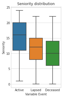
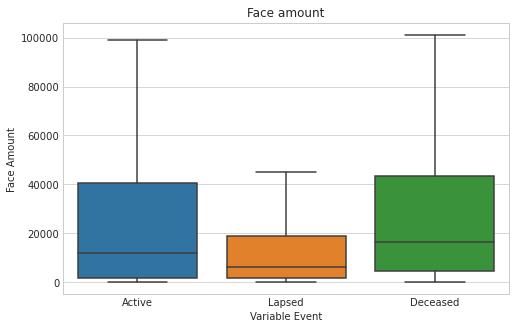
Figure 1: Seniorities and face amounts distributions

Without further analyzing the data, we can note several things. First, we can see that the mean censored seniority of 13.4 years is not equally distributed among our subjects. Active contracts tend to be older than lapsed ones, themselves older than policies that ended with the policyholder’s death. That emphasizes the importance of several contributions, and the apparent difference in seniority regarding the cause of the policy’s termination encourages a competing risks approach to analyze survival. Moreover, if we suspect lapse and death to be highly dependent on individual characteristics - such as the policyholder’s age - this also supports an individualized survival analysis. Eventually, we can see that the last face amount observed is significantly lower for lapsed policies. It confirms our first intuitions and the face amount will be included in our model.

Among the covariates introduced in Table 1, several play a central part in our two-step modeling approach. First, the competing risks survival analysis step where SENIORITY will be the response variable, and all other covariates, including individual data and financial flows, are potential explanatory variables. The binary classification second step aims at predicting the EVENT outcome with minor transformations explained in Section 3 below. It is equivalent to using STATE as a target variable, as they are entirely similar. As a result, all covariates are not utilized and our predictions are solely based on the covariates underlined in Table 1 as they appeared to be of interest to insurers.

3 Framework

This section describes a modeling approach that follows [45]’s work. Our contributions place our work in a framework that differs from it by being only future-oriented, by a precise and individualized analysis of retention probabilities and by choosing a classification framework instead of regression. We chose to use a majority of their existing notations here.
Usual lapse management models based on classification aim to predict whether a policyholder will lapse. They may perform very well at that specific task, but it only reflects some aspects of this economic problem. Indeed, the literature is clear ([2]), and many policyholders may be predicted as “lapsers” but may not be profitable to the insurance company if targeted. In that case, keeping such policyholders would be irrational, and an efficient model should not predict them as targets. Targeting policyholders is an economic problem that requires an economic measure to assess. We propose to consider a measure based on the discounted expected profit of all the policies, in other words, the sum of all $(\mathrm{CLVs})$. Optimizing a lapse, churn, or other prediction tasks with business-related measures is not new. However, to our knowledge, none of the existing approaches uses individualized future CLVs and models the profit of retention strategy by accounting for competing risks or using survival tree-based models.

$\mathrm{CLV}$ is a well-studied subject in marketing and business economics and has also been modeled in an insurance context. For a given subject $i$, her future $\mathrm{CLV}$ at horizon $T$ can be modeled as

$$\prescript{F}{}{C}LV_{i}\left(\boldsymbol{p}_{i},\boldsymbol{F}_{i},\boldsymbol{r}_{i},\boldsymbol{d},T\right)=\sum_{t=0}^{T}\frac{p_{i,t}F_{i,t}r_{i,t}}{\left(1+d_{i,t}\right)^{t}},$$ (1)

with $t$ in years, $t=0$ represents the last observation point for subject $i$. The quantity $p_{i,t}$ is her profitability ratio as a proportion of $F_{i,t}$, representing her face amount observed at time $t$. The quantity $r_{i,t}$ is the $i$-th subject’s probability of still being active at time $t$, and naturally, $d_{i,t}$ is the discount rate at time $t$, for subject $i$. We argue that both the profitability ratio and the discount rate should be as individualized as possible - either at the product or policy level - as $\prescript{F}{}{C}LV_{i}$ reflects the individualized risk of policyholder $i$ to the insurer. It is also worth mentioning that evaluating discount rates is well beyond the scope of this paper as it is complex and subject to significant judgment; for further details, we refer the astute reader to a variety of papers on the subject ([11], [50], [4]).

It is worth pointing out that $\prescript{F}{}{C}LV_{i}$ does not represent the global profit generated by subject $i$ from her policy’s first year until time $T$ as in [45]; it rather represents the future $T$ years of profit. $\prescript{F}{}{C}LV_{i}$ is not to be compared with the Cash Surrender Value but rather with the Fair Market Value (FMV) of the outstanding liabilities. The only difference with the latter is that $\prescript{F}{}{C}LV_{i}$ is based on the insurer’s knowledge of its portfolio, thus computed with its own profitability and discount parameters rather than with market-consistent considerations. Whereas the portfolio market value would consist of financial instruments that replicate the insurance liability cash flows. In our framework, the life insurer is more interested in maximizing its own realistic profitability rather than a sum of individual market values.
We suggest a model for the insurer’s estimated profit - or loss - resulting from a lapse management strategy (LMS). In order to do that, we will compare the expected value of the portfolio before and after applying a given strategy. We are aware that there could be infinite ways to design a retention campaign: offering a punctual incentive, recurrent services or more profit sharing, for instance. Here, we define what we will consider an LMS.

Definition 1 (Lapse management strategy)

A T-years lapse management strategy is modeled by the offer of an incentive $\delta_{i}$ to subject $i$ if she is targeted. The incentive is expressed as a percentage of her face amount and should not exceed the profitability ratio $p_{i,t}$, at any time point $t$. Contacting the targeted policyholder has a fixed cost $c$ and after contact, the incentive is accepted with probability $\gamma_{i}$. A targeted subject who accepts the incentive will be considered as an “acceptant” who will never lapse. In our dataset, any subject that has never been observed to lapse is considered as an “acceptant” and her probability of being active at year $t\in[0,T]$ is denoted $r_{i,t}^{\text{acceptant}}$. Conversely, a subject who refuses the incentive and prefers to lapse will be considered as a “lapser”. In our dataset, a subject is labeled as a lapser whenever she has been observed to lapse at year $t=0$, and her probability of being active at year $t$ is denoted $r_{i,t}^{\text{lapser}}$. A lapse management strategy is uniquely defined by the parameters $(\boldsymbol{p},\boldsymbol{\delta},\boldsymbol{\gamma},c,T)$ It is to be noted that even if the framework involves a time dimension, it is still a static approach: the insurer would run all analyses on its portfolio at one given time and apply an appropriate LMS immediately.
Even if this definition is already a simplification of any real-life insurance retention strategy, various constraints and the data and tools at the insurer’s disposal do not always allow to conduct such a study. In the following section, we consider a simplified version of this framework by assuming that $p_{i,t},F_{i,t}$, and $d_{i,t}$ remain constant across time, and denoted $p_{i}$, $F_{i}$ and $d_{i}$ hereafter, with $F_{i}$ being the most recent face amount observed for subject $i$. Moreover, we set $\gamma_{i}$ and $\delta_{i}$ to be the same for all subjects and denoted as $\gamma$ and $\delta$ hereafter. The constraint that $\delta<min(p_{i})$ detailed in Definition 1 still holds. Finally, the last observed state of subject $i$ is denoted $y_{i}$, with $y_{i}=1$ if the policy is lapsed, $y_{i}=0$ otherwise.

With those considerations, we can then define the control portfolio’s future value as

$$\prescript{F}{}{C}PV (\boldsymbol{p},\delta,\gamma,c,T)=$$ (2)

$$\phantom{aa}\sum_{i=1}^{n}\prescript{F}{}{C}LV_{i}\left({p}_{i},F_{i},\boldsymbol{r}^{\text{acceptant}}_{i},d_{i},T\right)\cdot\mathbf{1}\left(y_{i}=0\right)$$

$$+\sum_{i=1}^{n}\prescript{F}{}{C}LV_{i}\left({p}_{i},F_{i},\boldsymbol{r}^{\text{lapser}}_{i},d_{i},T\right)\cdot\mathbf{1}\left(y_{i}=1\right).$$

It represents the hypothetical value of the portfolio, considering that:

• every subject that did not lapse up to her last observation point - $y_{i}=0$ at $t=0$ - has a vector of retention probabilities of $\boldsymbol{r}^{\text{acceptant}}_{i}$;

• every subject that has been observed to lapse - $y_{i}=1$ at $t=0$ - has a vector of retention probabilities of $\boldsymbol{r}^{\text{lapser}}_{i}$

Remark 1

It is important to note that this does not reflect the actual future value of the portfolio - as the future CLV of lapsers should be $0$ - but rather its hypothetical expected future value given the nature (lapser or not) of every subject but not their actual states (actually lapsed or not). It represents this hypothetical future CLV of all subjects if no customer relationship management about lapses is carried out.

A classification algorithm would take the lapse indicator $y_{i}$ as a target variable and yield predictions $\hat{y}_{i}$. Given a lapse management strategy and such a classification algorithm, we define the lapse managed portfolio future value by

$$\prescript{F}{}{L} MPV(\boldsymbol{p},\delta,\gamma,c,T)= \phantom{aaaaaaaiii}\sum_{i=1}^{n}\prescript{F}{}{C}LV_{i}\left({p}_{i},F_{i},\boldsymbol{r}^{\text{acceptant}}_{i},d_{i},T\right)\cdot\mathbf{1}\left(y_{i}=0,\hat{y}_{i}=0\right) \phantom{aaaaaiii}+\sum_{i=1}^{n}\prescript{F}{}{C}LV_{i}\left({p}_{i},F_{i},\boldsymbol{r}^{\text{lapser}}_{i},d_{i},T\right)\cdot\mathbf{1}\left(y_{i}=1,\hat{y}_{i}=0\right) \phantom{aaaaaiii}+\sum_{i=1}^{n}\prescript{F}{}{C}LV_{i}\left({p}_{i}-\delta,F_{i},\boldsymbol{r}^{\text{acceptant}}_{i},d_{i},T\right)\cdot\mathbf{1}\left(y_{i}=0,\hat{y}_{i}=1\right) \phantom{aaaai}+\gamma\cdot\sum_{i=1}^{n}\prescript{F}{}{C}LV_{i}\left({p}_{i}-\delta,F_{i},\boldsymbol{r}^{\text{acceptant}}_{i},d_{i},T\right)\cdot\mathbf{1}\left(y_{i}=1,\hat{y}_{i}=1\right) +(1-\gamma)\cdot\sum_{i=1}^{n}\prescript{F}{}{C}LV_{i}\left({p}_{i},F_{i},\boldsymbol{r}^{\text{lapser}}_{i},d_{i},T\right)\cdot\mathbf{1}\left(y_{i}=1,\hat{y}_{i}=1\right) \phantom{aaaaaiii}-\sum_{i=1}^{n}c\cdot\mathbf{1}\left(\hat{y}_{i}=1\right).$$ (3)

Clearly, the sums appearing in the formulas above could be grouped to make them more concise. We chose not to do so for the sake of visualization: we can distinctly see each possible case in each summand.
Then, we define the economic metric of the algorithm as the retention gain, the future profit generated by the retention management strategy over $T$ years as

$$RG(\boldsymbol{p},\delta,\gamma,c,T)=\operatorname{\prescript{F}{}{L}MPV}(\boldsymbol{p},\delta,\gamma,c,T)-\prescript{F}{}{C}PV(\boldsymbol{p},\delta,\gamma,c,T),$$ (4)

which can be simplified as

$$RG(\boldsymbol{p},\delta,\gamma,c,T)= \sum_{i=1}^{n}\Biggr{[}\gamma\Big{[}\prescript{F}{}{C}LV_{i}\left({p}_{i}-\delta,F_{i},\boldsymbol{r}^{\text{acceptant }}_{i},d_{i},T\right)$$ (5)

$$-\prescript{F}{}{C}LV_{i}\left({p}_{i},F_{i},\boldsymbol{r}^{\text{lapser }}_{i},d_{i},T\right)\Big{]}\cdot\mathbf{1}\left(y_{i}=1,\hat{y}_{i}=1\right)$$

$$-\prescript{F}{}{C}LV_{i}\left(\delta,F_{i},\boldsymbol{r}^{\text{acceptant }}_{i},d_{i},T\right)\cdot\mathbf{1}\left(y_{i}=0,\hat{y}_{i}=1\right)\Biggr{]}$$

$$-\sum_{i=1}^{n}c\cdot\mathbf{1}\left(\hat{y}_{i}=1\right).$$

This evaluation metric can now be derived into an individual retention gain measure. More specifically, we define $z_{i}$ as

$$z_{i}=\begin{cases}-\prescript{F}{}{C}LV_{i}\left(\delta,F_{i},\boldsymbol{r}^{\text{acceptant }}_{i},d_{i},T\right)-c&\text{ if }y_{i}=0\\ \text{ }\\ \gamma\cdot\Big{[}\prescript{F}{}{C}LV_{i}\left(p_{i}-\delta,F_{i},\boldsymbol{r}^{\text{acceptant }}_{i},d_{i},T\right)&\text{ if }y_{i}=1\\ \phantom{ii}-\prescript{F}{}{C}LV_{i}\left(p_{i},F_{i},\boldsymbol{r}^{\text{lapser }}_{i},d_{i},T\right)\Big{]}-c.\end{cases}$$ (6)

That last equation can seem obscure at first glance. It simply assigns to each individual the expected profit or loss that would result from targeting her with a given lapse management strategy. A positive amount for subject $i$ means that targeting her would generate profit, whereas a negative one would lead to a loss for the insurer. We can take the example of a hypothetical scenario where $p_{i}=3\%$, $\delta=0.05\%$, $\gamma=10\%$ and $c=10$ euros. It would generate $z_{i}$s taking values from $-234,614$€ to $53,066$€ with a mean of $-218$€ and a median of $-55$€. Different scenarios would result in very different distributions for the $z_{i}$’s.

Eventually, we define $\tilde{y}_{i}$ as a binary target variable indicating for policyholder $i$ if the individual expected retention gain resulting from a given retention strategy is a profit or a loss. More specifically, we define $\tilde{y}_{i}$ as

$$\tilde{y}_{i}=\left\{\begin{array}[]{l}1\text{ if }z_{i}>0\\ 0\text{ if }z_{i}\leq 0\end{array}.\right.$$ (7)

Remark 2

A subject in the dataset for which $y_{i}=0$ would produce $\tilde{y}_{i}=0$, whereas one for which $y_{i}=1$ could produce $\tilde{y}_{i}=0$ or $\tilde{y}_{i}=1$. In other words, it is never profitable for the insurer to offer an incentive to a subject that would not have lapsed. On the other hand, offering that same incentive to a lapser can be profitable. However, depending on the subject’s features and the lapse management strategy parameters, it can also lead to a loss.

We can now include $\tilde{y}_{i}$ as a new binary target variable in our models and directly consider $RG$ as the global evaluation metric in the tree-based models we consider.
We can now compare two models: the classical one with $y_{i}$ as a target variable and accuracy as the evaluation metric; and the CLV-augmented one with $\tilde{y}_{i}$ as a target variable and $RG$ as the evaluation metric.

Intuitively, the former tries to predict whether a policyholder will lapse and tune its parameters by minimizing the misclassification rate. On the other hand, the latter aims at predicting whether applying a given retention strategy to the $i$-th individual will be profitable for the insurer and tune its parameters by maximizing the global expected retention gain.

4 Methodology

In Section 3, we described a business-oriented framework, augmenting lapse management strategy with an evaluation metric based on the future CLV of every subject. Evaluating this metric requires computing $r^{\text{acceptant}}$ and $r^{\text{lapser}}$, the matrices of size $(n,T+1)$ containing for every subject, survival probabilities that we detail below. This individual survival analysis differs from [45]’s work where $r^{\text{lapser}}$ is estimated globally and takes the same value for every policyholder regardless of their characteristics and where $r^{\text{acceptant}}=1$ for any subject and at any time, ignoring the fact that an “acceptant”’s policy can end with the policyholder’s death.
Given this framework, we propose a two-step methodology: firstly, we detail how this survival analysis is carried out to model those retention parameters, and secondly, we explain how we use them for training tree-based classification models.

4.1 Step 1: Modeling $r^{\text{acceptant}}$ and $r^{\text{lapser}}$

We recall that a given subject’s policy can end with lapse or death, and the policy is considered active if competing events are yet to occur. Furthermore, while a lapser’s policy can end with lapse or death, whatever comes first, an acceptant one can only end with death.
$r^{\text{lapser}}$ represents the probability that the policy of subject $i$ is still active at time $t$, given that the subject is labeled as a lapser - $\text{EVENT}=1$ - at $t=0$. Predicting these overall conditional survival probabilities with competing risks can be achieved by creating a combined outcome: the policy ends with death or lapse, whichever comes first. To compute $r^{\text{lapser}}$ in practice, we recode the competing events as a combined event. This approach is compatible with any survival analysis method regarding statistical guarantees.

Conversely, $r^{\text{acceptant}}$ represents the probability that the policy of subject $i$ is still active at time $t$, given that the subject is not labeled as a lapser - $\text{EVENT}=0$ or $2$ - at $t=0$. This estimation is more complex as we must dissociate the risks of lapse and death. These causes being mutually exclusive, a competing risks methodology is well-suited to estimate $r^{\text{acceptant}}$ [42].

It is also important to note that here, $r^{\text{lapser}}$ is modeled on subjects that have lapsed in the past - they may have been offered an incentive in the past, this is unknown - and not on subjects that have been offered an incentive that they declined. Our framework makes the implicit hypothesis that both behaviors are alike. It is more intuitive for $r^{\text{acceptant}}$ as a subject that has not lapsed in the past would have accepted any incentive if offered.

4.1.1 Competing risks frameworks

We are aware that improvements of our model over [45]’s approach, require the analysis of both the risks of lapse and death, thus a competing risk setting. As detailed in Appendix A.1, several regression models exist to estimate the global hazard and the hazard of one risk in such settings: cause-specific and subdistribution models. They account for competing risks differently, obtaining different hazard functions and thus have distinct advantages, drawbacks and interpretations. These differences are discussed in [47], where the authors also considered a competing risk framework for lapse prediction.
After discussions detailed in Appendix A.1, the simplicity of a cause-specific approach and the fact that it can be adapted to any survival method, including tree-based ones, oriented our choice towards it. We then computed $r^{\text{acceptant}}$ and $r^{\text{lapser}}$ with three different methods - Cox model, Random Survival Forest and Gradient Boosting Survival Model - and retained the best one. These methods are shortly described in the following sections.

4.1.2 Cox proportional hazard model

One of the most common survival models is the Cox proportional hazard (CPH) model ([14]). It postulates that the hazard function can be modelized as the product of a time-dependent and a covariate-dependent functions. The hazard function at time $t$ for subject $i$ with covariate vector $\boldsymbol{X_{i}}$, under Cox proportionnal hazard model can be expressed as

$$\underbrace{\lambda(t|X_{i}^{1},X_{i}^{2},\dots)}_{\text{hazard function}}=\lambda(t|\boldsymbol{X_{i}})=\overbrace{\lambda_{0}(t)}^{\text{baseline hazard}}\underbrace{e^{\overbrace{\left(\boldsymbol{X_{i}}\cdot\beta_{i}\right)}^{\text{log-partial hazard}}}}_{\text{partial hazard}}.$$

It is crucial to note that in this model, the hazard function is the product of the baseline hazard, which only varies with time, and the partial hazard, which only varies depending on the covariates. The parameters of this model are the $\beta$, and they can easily be estimated with a maximum likelihood approach. Their estimation can be carried out without having to model $\lambda_{0}(t)$ - which is why CPH is considered semi-parametric.
We use Python and lifelines ([17]) to implement it. We specify a spline estimation for the baseline hazard function. We select the covariates and model parameters using AIC ([1]) and use the concordance index ([30]) to compare CPH to other models. The concordance index - or Harrel’s c-index or simply c-index - is a metric to evaluate the predictions made by a survival model. It can be interpreted as a generalization of the area under a receiver operating characteristic (ROC) curve ([29]) - or AUC - in a survival setting with censored data.

4.1.3 Random Survival Forest

Survival trees have been extensively studied for a long time, and a complete review of such existing methods up to 2011 can be found in [5]. The most important thing to understand is that a survival tree can be created by modifying the splitting criterion of a regular tree. Most survival tree algorithms are designed with a split function that aims to maximize the separation of the resulting child nodes in terms of survival profiles. This separation between nodes is estimated by maximizing the log-rank statistic ([46; 43]). Each terminal node of a survival tree contains a survival profile from which we can derive the survival and cumulative hazard function.

An RSF is the counterpart of a random forest (see Appendix A.2.2) for such survival trees. It has been developed in [35] and extended for competing risks a few years after ([36]). A prediction with RSF for a given subject is made by getting his/her survival profile in each tree in the forest. His/her corresponding survival and cumulative hazard function are estimated in each tree with Kaplan-Meier and Nelson-Aalen estimators, respectively. Eventually, the aggregation of those single-tree estimates constitutes the RSF’s prediction.

We use Python and sksurv ([52]) to implement RSF, and we tune and evaluate our model using the concordance index.

Remark 3

Sksurv allows us to use RSF with a cause-specific consideration of the competing risks. To this day, sksurv does not have a subdistribution competing risks model, whereas its R implementation randomForestSRC does ([34]).
Moreover, a severe limitation of that approach is that predictions can only be made at time points observed in the training set. Concretely, this prevents us from using RSF to extrapolate survival and hazard functions to unobserved time points.

4.1.4 Gradient Boosting Survival Model

In the same way Random Forest has a survival counterpart, this is also true for Gradient Boosting approaches. An essential distinction between classical boosting algorithms (see Appendix A.2.3) and Gradient Boosting Survival Model (GBSM) lies in its loss function. The loss function that we use with GBSM is the partial likelihood loss of a CPH model, and the optimization in such a model is achieved by maximizing a slightly modified log-partial likelihood function,

$$\arg\min_{f}\quad\sum_{i=1}^{n}\delta_{i}\left[f(\boldsymbol{X_{i}})-\log\left(\sum_{j\in{g}_{i}}e^{(f(\boldsymbol{X_{j}}))}\right)\right],$$

where $\delta_{i}$ is the event indicator and $f(\boldsymbol{X_{i}})$ is GBSM’s prediction for the $i$-th subject, with a covariate vector $\boldsymbol{X_{i}}$. ${g}_{i}$ is the tree leaf including subject $i$.
Similarly to RSF, we use Python and sksurv ([52]) to implement GBSM. We tune and evaluate our model using the concordance index. Remark 3 also applies here.

4.1.5 Final modeling choice

Our analysis shows that, based on concordance index, RSF and GSBM both outperformed a semiparametric Cox model in our study case. Regarding interpretability, we note that the feature importance analysis is very similar between the three models. All the details about the final concordance index scores, covariates importance and various plot for further analysis are available in Appendix A.2.

In the following sections, we decide to retain GBSM for the modeling of $r^{\text{acceptant}}$ and $r^{\text{lapser}}$ as it has the best concordance index.

Remark 4

As this study aims to be business-oriented and favor real-life decision-making, it is crucial to note that the computation times for fitting these different models are very different and could potentially be a huge constraint for real operational deployment. Specific computation times differ greatly depending on various factors, such as the number of subjects or features considered, the computation power or parallelization ability at disposal, for instance. However, we can still give here an order of magnitude for those differences. If the tuning and fitting process for CPH can last a few tens of seconds, it lasts hours for RSF and tens of hours for GBSM.

4.2 Step 2: Classification tasks

Our work focuses on lapse management with tree-based models. It aims to answer the question: which policyholders would be worth targeting with a lapse management strategy to maximize the expected T-year profit for the insurer? We will consider a single tree built with Breiman’s CART algorithm, Random Forest, XGBoost, and RE-EM trees. The following sections detail how those different approaches work. Those models will be compared on two different classification tasks; and tuned with two different evaluation metrics, a statistical metric and a business-related one.

On $y_{i}$

First, we will use a classical lapse prediction framework to model the policyholder’s behavior. Each policyholder will be labeled as a lapser or a non-lapser with a binary outcome $y_{i}$. Our first batch of models will be trained with $y_{i}$ as a response variable and produce predictions $\hat{y}_{i}$. $\operatorname{Accuracy}(y,\hat{y})$, which is undoubtedly the most intuitive performance measure for binary classification, is defined as the proportion of correctly predicted observations over all observations. It is widely used for churn analysis and appears to be a satisfying performance measure for relatively balanced outcomes - 22% of all observed subjects being lapsers - in binary classification problems. We will use it as an evaluation metric in a 10-fold cross-validation step for tuning our models.
We know that more advanced evaluation metrics are available for binary classification, including the recall, the $\operatorname{F_{\beta}}$ score family ([13]), the AUC under the ROC or under the Precision-Recall curve, the Brier Score ([8]) and lift curve. They are standard evaluation metrics in classification and provide valuable insights into the model’s performance, they are also frequently used in the applied binary classification literature, especially in the presence of a significant imbalance in the data ([31]). However, in this paper, the mildness of the imbalance of $y_{i}$ and our will to compare a customer-centered framework to representative real-world practices encourages us to use accuracy as a comparison. One of the goals of this article is to demonstrate that some of the current practices in real-world applications, based on statistical metrics such as accuracy can be significantly improved by considering a profit-driven target variable and evaluation metric. We are aware that accuracy may not be an optimal choice of evaluation metric for binary prediction in general and churn or lapse analysis specifically, but it seems representative of what practitioners use (see Table 2 from [19] for example), as it is suggested in [45]. We do not aim at comparing our framework against the best existing methods but rather against the most representative. Nevertheless, the numerical results of Table 3 have also been obtained with recall, F1-score, and AUC for tuning and cross-validation and some are available in Appendix A.4: the conclusions obtained with such measures are similar to those obtained with accuracy. Thus, in this article and as in [45], we will only select, evaluate and discuss the models in the light of accuracy.

On $\tilde{y}_{i}$

Secondly, we will use the CLV-Augmented lapse prediction framework, detailed in Section 3. Each policyholder will be labeled as a targeted lapser or a non-targeted policyholder with the binary outcome $\tilde{y}_{i}$ and prediction for that outcome are denoted $\hat{\tilde{y_{i}}}$.

Remark 5

Note that whenever $y_{i}=0$, we also have $\tilde{y}_{i}=0$. In other words, if subject $i$ does not intend to lapse, it is never worth proposing her an incentive: the subject will accept it with probability $1$ and would not have lapsed.
On the other hand, when $y_{i}=1$, it corresponds to either $\tilde{y}_{i}=1$ or $\tilde{y}_{i}=0$. In other words, if subject $i$ is labeled as a lapser, it does not necessarily mean it is worth targeting her. From the insurer’s point of view, some policies are better off lapsed. $\tilde{y}$ can be seen as a more detailed version of $y_{i}$ as it carries not only behavioral information regarding lapse but also a profitability one.

We thus train a second batch of models with $\tilde{y}_{i}$ as a response variable. We use $RG$ as an evaluation metric in a 10-fold cross-validation step for tuning these models. Summary of our methodology: First, we train a CART, RF and XGBoost models with $y_{i}$ as a binary target variable and accuracy as a tuning evaluation metric.
Then we train them with $\tilde{y}_{i}$ as a binary target variable and $RG$ as a tuning evaluation metric.
Finally, we train and test all six models on different random samples of our dataset and keep track of the model’s classification performance on all of them and for various retention strategies for comparison’s sake. The sections below briefly introduce the tree-based model we selected before displaying how they performed in various lapse management scenarios.

4.2.1 CART

CART (Classification And Regression Trees) is an algorithm developed by [7] that consists of recursively partitioning the covariate space. It is a widespread, intuitive and flexible algorithm that handles regression and classification problems.

4.2.2 Random forest

A natural idea to correct CART’s instability and enhance its prediction accuracy is the aggregation of a significant number of single trees, each grown on different subsamples of the dataset. A random forest (RF by [6]) is a tree-based bagging procedure where each tree is grown on randomly drawn observations and contains splits considering only randomly drawn covariates.

4.2.3 XGBoost

Other tree-based approaches have been designed to reduce the instability of a single-tree model. Model boosting is an adaptative technique, first developed by Freund et Shapire ([22]), that does not rely on the aggregation of independent weaker models but rather on the aggregation of weak models built sequentially, one after the other. XGBoost ([12]) is a widespread and performant tree-boosting model that relies on a gradient-boosting step and provides a very optimized parallelized procedure. It is considered a state-of-the-art library for various prediction problems.

The interested reader can find more detailed explanations about CART, RF and XGBoost mechanisms in the aforementioned references. For these modeling approaches, we used Python and sklearn ([51]).

5 Real-life application

Based on the real life-insurance dataset at our disposal (described in Section 2), we use the survival model we selected and estimate $r^{\text{acceptant}}$ and $r^{\text{lapser}}$ for every individual. This allows us to compute the individual CLVs, RGs, $z_{i}$’s and $\tilde{y}_{i}$. We have already defined what a strategy is (see Definition 1), and we can thus apply our classification methodology to various retention strategies.

5.1 Considered lapse management strategies

The strategies considered are based on several criteria. First, we selected realistic strategy parameters and time horizons based on actual retention campaigns led by life insurers. Moreover, we chose to present strategies that illustrate the exhaustive list of conclusions and discussions that are carried out in the next section. Finally, we also incorporated strategies that are “obviously bad” in the sense that such strategies would necessarily lead to a loss for the insurer. Such extreme scenarios will supplement our discussions. In any case, we consider $p_{i}$ and $d_{i}$ to be constant in our application, as both those parameters were not estimated at the individual level by the life insurer that provided with the dataset.
Results related to the 64 considered LMS are given in Appendix A.5. Our analysis showed that all considered LMS results can be split into 5 categories depending on how applying our framework impacted their expected retention gain over a naïve targeting. We have realistic profitable strategies that are improved by our framework, but also highly loss-inducing, moderate loss-inducing, highly profitable and unrealistically highly profitable strategies. We refer to the LMS displayed in Table 2 as representative strategies as they all belong to one of those categories. Numerical results regarding the most representative strategies can be found in Section 5.2 and related comments on how to read these tables are given in Section 5.3.

Scenarios p $\delta$ $\gamma$ c d T A-1 2.50% 0.04% 25% 10 1.50% 5 A-5 2.50% 0.04% 5% 10 1.50% 5 A-25 5.00% 0.10% 25% 10 1.50% 5 B-6 2.50% 0.08% 10% 10 1.50% 20 B-27 5.00% 0.20% 20% 100 1.50% 5

Table 2: Insightful LMS

5.2 Numerical results

N° time (s) Model % target diff (% of 1’s) Accuracy Retention gain RG/target Improvement $y_{i}$ $\tilde{y}_{i}$ $y_{i}$ $\tilde{y}_{i}$ $y_{i}$ $\tilde{y}_{i}$ A-1 4949 CART 62.6% (8.2%) 92.3% 85.3% 114 661 219 655 4.48 38.20 91.6% RF 92.9% 85.4% 232 314 287 884 9.82 56.65 23.90% XGB 93.4% 85.8% 243 365 324 952 9.61 54.64 33.50% A-5 4753 CART 86.7% (2.9%) 92.3% 83.6% - 514 477 - 112 372 - 20.08 - 86.48 78.20% RF 92.9% 83.4% - 323 544 - 3 937 - 13.65 - 28.28 98.80% XGB 93.4% 83.3% - 383 004 0 - 15.14 0 100.00% A-25 5379 CART 31.0% (15.2%) 92.3% 89.2% 4 160 423 3 882 623 162.44 241.06 -6.70% RF 92.9% 89.5% 4 018 432 3 666 219 169.65 249.54 -8.80% XGB 93.4% 90.0% 4 455 108 4 410 629 176.09 267.87 -1.00% B-6 5906 CART 36.6% (13.9%) 92.3% 88.8% 705 721 922 490 27.69 60.21 30.70% RF 92.9% 88.9% 1 352 182 1 269 349 57.11 97.63 -6.10% XGB 93.4% 89.6% 1 342 882 1 428 722 53.09 96.76 6.40% B-27 4811 CART 73.9% (5.7%) 92.3% 84.3% - 694 436 751 404 - 27.16 226.99 208.20% RF 92.9% 84.4% - 13 512 1 018 369 - 0.51 356.48 7637.00% XGB 93.4% 84.7% - 38 050 1 253 252 - 1.55 345.94 3393.70%

Table 3: Means of the results obtained on considered LMS

5.3 Comments

Several terms in the two previous tables need to be explained. “% target diff” represents how different $y$ and $\tilde{y}$ are. It is the percentage of subjects for which $y_{i}=1$ and $\tilde{y}_{i}=0$: in other words, the proportion of lapsers not worth targeting with a given strategy. The quantity “% of 1’s” represents the proportion of ones in $\tilde{y}$ the target variable. It is to be compared with the 22% of ones in $y$: the proposed framework’s imbalance increases with “% target diff”.
Then the table shows the 10-fold cross-validated mean accuracies, retention gains and RG/target with two methodologies: the columns denoted $y_{i}$ represent the metrics obtained by a model with $y_{i}$ as a response variable and accuracy as an evaluation metric, and the columns denoted $\tilde{y}_{i}$ represent the metric obtained by a model with $\tilde{y}_{i}$ as a response variable and $RG$ as an evaluation metric.
RG/target represents the achieved retention gain for every targeted individual, for $y_{i}$, it is $RG/\sum_{i}\hat{y_{i}}$, for $\tilde{y}_{i}$ it is $RG/\sum_{i}\hat{\tilde{y_{i}}}$. Eventually, “Improvement” represents the percentage of improvement between the $RG$ obtained with a classification on $y_{i}$ and the gain obtained with a classification on $\tilde{y}_{i}$. As the reported financial information was distorted for confidentiality reasons (see Section 2), relative measures such as “Improvement” are certainly more informative than absolute ones such as $RG$.
Some LMS are worth focusing on. For every strategy, we display its 10-fold cross-validated results: 10% of the dataset acting as an out-of-sample validation set at every fold. Every model is tuned by cross-validation within every fold. The boxplots below summarize some typical key results illustrated by several strategies. Those results will be discussed in Section 6.

Figure 2: Strategy n°A-1: (Positive result on $y_{i}$ and an improved result on $\tilde{y}_{i}$.)

Figure 3: Strategy n°A-5: (Very negative result on $y_{i}$ and a loss-limiting result on $\tilde{y}_{i}$.)

Figure 4: Strategy n°B-27: (Negative result on $y_{i}$ and positive one on $\tilde{y}_{i}$)

Figure 5: Strategy n°B-6: (High positive result on $y_{i}$ slightly improved with $\tilde{y}_{i}$.)

Figure 6: Strategy n°A-25: (Results on $y_{i}$ better than results on $\tilde{y}_{i}$.)

Remark 6

With considerable computation power and great parallelization, the results for all strategies - see other strategies in Appendix A.5 - were obtained with a wall time of less than 4 days and a CPU time of more than 100 days.

6 Discussion

6.1 General statements

As expected and shown in the actuarial literature, RF and XGBoost perform globally better than CART regarding mean accuracy and RG. It is true for all LMS considered in Table 10. Globally, XGBoost is more consistent and is the best model in most scenarios, both with and without the CLV-based measure. It is only outperformed by RF in strategies n°A-7, A-11, A-14, A-29, B-7, B-14 and B-31.
As expected, by design, the vast majority of strategies, including all the realistic ones, show that a classification on $\tilde{y}_{i}$ produces a targeting that yields better RG than a classification on ${y}_{i}$. Conversely, a classification on $y_{i}$ produces a targeting that delivers better accuracies regarding whether a policyholder will churn than a classification on $\tilde{y}_{i}$. These results were expected because of the models’ respective objectives. Even if it is not surprising, it once again shows that for an insurer, lapse prediction and lapse management strategy are two very different prediction problems, often treated as similar ones.

Our CLV-augmented model shows different behavior depending on the strategy considered. As highlighted by Figure 2, a model on $y_{i}$ is greatly improved by our framework regarding RG and RG/target. Conversely, its accuracy in lapse prediction is not optimal.
An attractive property of our framework can be observed in Figure 3: it yields loss-limiting targeting. When the LMS considered is too aggressive, it will usually prefer to predict that an LMS should not be applied at all ($\forall i,\hat{\tilde{y_{i}}}=0$), thus generating a $RG$ around 0€. This is made evident in some extreme strategies (LMS n°A-5, A-15, B-11, B-13 and B-16) and explains the presence of 0’s in Table 3.
On less extreme strategies, it shows to yield substantial improvement when classification on ${y}_{i}$ gives negative RG. That observation confirms what was already pointed out by [45]: it can even turn a negative $RG$ into a positive one (see LMS n°A-8, B-8, B-12, B-23 and B-27 (Figure 4)) .
Our framework also improves a strategy where a classification on ${y}_{i}$ gives high RG. However, the improvement decreases as the difference between the total number of lapsers and the number of lapsers that would be profitable if retained is sizeable. An example of that is shown in Figure 5.

Finally, we can generate LMS for which our framework does not improve the expected RG. It is the case in LMS n°A-13, A-18 or A-27 (See e.g Figure 6). In LMS n°A-13, we can see that the mean of the RG is not improved, but the median is. In all those cases, the RG per target produced by the CLV-augmented model is greatly improved, indicating that a CLV-augmented strategy prefers to target fewer policyholders but only those who would generate high future profits. This last observation explains why a CLV-augmented LMS generates higher RGs when the cost of contact c is considerable. Indeed, the more costly a contact is, the more precise and specific a targeting strategy should be.

Generally, we can collate the results of various LMS - excluding LMS n°B-27 that has a very high improvement ratio - to obtain a mean performance of our framework.

The average observed RG improvement of a CLV-augmented framework over the classical lapse one is 57,9%. If we weigh these results by the expected RGs, the average improvement is still 31,7%. As a comparative result, it is reported in Section 6.2 of Loisel et al.’s work ([45]) that they obtain improvements over that same classical framework between 18% and 26%, depending on the considered strategies. This emphasizes that by extending their work, we seem to improve on their results. Obviously, as we were not able to compare our results on the same data and strategies, and because our definitions of $RG$ differ, such a conclusion is to be treated cautiously.

6.2 Marketing decision making

We already pointed out that the improvement of a lapse management strategy including CLV grows with the proportion of lapsers with a negative CLV (see Appendix A.3). Models resulting from our framework do not consider them as good targets. In fact, there is a Pearson correlation coefficient of 77% between RG improvement and the proportion of target differences among the LMS detailed in Table 10. Of course, as the improvement ratio has no clear interpretation in some cases, this analysis should be carried out in more depth, separating the cases where both RG - with and without the inclusion of CLV - are positive from the cases where one of them is negative. By doing so, we observe that the Pearson correlation coefficient for LMS yielding positive RG regardless of the inclusion of CLV is even higher: 83%.

In terms of targeting, it seems crucial to understand what differentiates a subject for which $y_{i}=1$ and $\tilde{y}_{i}=0$ from the others. An investigation of such policyholder profiles can be carried out for every lapse management strategy. We take the example of LMS n°A-1, where 62,6% of policyholders were in that case (see Section 5.2). With that strategy, the profile of non-targeted lapsers indicates that

• 57.2% of them are men, similar to the entire dataset,

• 76.4% of them contracted product n°1 whereas 72% of all policyholders chose it,

• the mean seniority of their policy is 10.4 years compared to the 13.4 years for the complete dataset,

• the mean face amount of such policies is 12,156, whereas the average face amount for all considered policies is 40,263.

In that strategy, our framework indicates that marketing efforts on low seniority policyholders with low face amount policies are inefficient. Of course, this conclusion is only valid for the considered LMS; however, our framework allows us to conduct such analysis for any LMS and interpret the results at an individualized level.

6.3 Management rules decision making

Sensitivity analysis of those results can highly benefit management rules decision-making. This framework serves as a tool that compares future hypothetical lapse management strategies in order to choose the best one - among realistic scenarios -. It can also be used to tune a given strategy by answering questions like:

• For which incentive $\delta$ the retention strategy becomes profitable ?

• For which acceptance probability $\gamma$ the retention strategy becomes profitable ?

• With a given budget, what is the optimal list of policies that should be targeted?

• At which horizon $T$, the retention strategy become profitable ? In other words, when can the insurer expect a return on investment?

Answering these questions constitutes a 1-parameter sensitivity analysis. In our framework, six parameters influence the expected retention gain $(p,\delta,\gamma,c,d,T)$.
We can argue that among them are three structural parameters that are insurer’s dependent and not linked to the external state of the world: $\delta$, $\gamma$ and $c$. Among them, the contact cost $c$ is more or less fixed and can not be easily changed by the insurer. Conversely, $\delta$ and $\gamma$ are to be chosen by the insurer. Moreover, they also are correlated with management and commercial efficiency - an efficient campaign impacts the final $\gamma$ - and correlated together: the higher the incentive $\delta$, the higher the probability of acceptance $\gamma$.
By fixing all other parameters and trying various combinations of $\delta$ and $\gamma$ we obtain the following 3D surfaces.
Figure 7: 3d plot ($\delta$, $\gamma$, RG)

This surface is not surprising and indicates that the higher the acceptance rate and the lower the incentive, the higher the retention gain. The surface gradient can give powerful insights regarding the most efficient commercial efforts to make: is it better for the insurer to propose lower incentives and manage to conserve the same acceptance probability or to put commercial effort into improving the acceptance probability for the same proposed incentive? This surface directly addresses this question.

Remark 7

Of course, the interdependency of those parameters should make some part of this surface unrealistic from a management decision-making point of view. The insurer should consider such dependencies when designing a lapse management strategy. Among the six parameters are also three conjectural parameters that depend on the external state of the world: the insurer’s profitability $p$ (that depends on competition, macroeconomic considerations or regulation), the discount rate $d$ and the time horizon $T$ (that can be driven by the insurer’s vision but also by regulation: the ORSA time horizon with the strategic and the long-term business planning time horizon should be both considered). Among them, we chose to fix $p$ and let $d$ and $T$ vary. Moreover, $p$ and $T$ are obviously interdependent and considered through the management’s prospective view of the conjecture’s evolution. A given interest rate scenario should represent a curve on the following surface.
Figure 8: 3d plot (d, T, RG) This surface is less smooth than the one displayed in Figure 7 and seems to indicate a more unstable relationship between RG and the conjectural parameters. An explanation of that behavior can be that those surface points are generated by running our framework on a random subsample of our dataset, for computation time considerations. Generating the same surface with more policyholders is likely to give a smoother behavior.

Remark 8

Of course, the interdependency of $T$ and $d$ should make some part of this surface unrealistic from an actuarial point of view. Actuarial rate projections would give precise plausible scenarios on this surface. Such considerations should be taken into account by the insurer when designing a lapse management strategy.

Remark 9

The insurer can also use our framework to measure the retention gain to be expected at different time horizons obtained by existing retention campaigns. In that case, the insurer would have to neutralize the effect of the existing LMS in order to estimate the control portfolio’s future value. We leave this remark as future work for applied risk management research.

7 Conclusion and perspectives

The work carried out in this paper shows that including CLV in lapse management strategy can largely benefit an insurer’s decision-making ability regarding lapse management strategy. We showed that survival tree-based models can outperform parametric approaches in such actuarial contexts. Then, our comparison of tree-based models on different lapse management strategies indicated that our CLV-based framework leads to increased predicted gains for any realistic scenario and acts as a loss-limiting targeting approach, regardless of the retention strategy. Moreover, the global results obtained in Section 6.1 show that our approach significantly improves on existing ones. Eventually, the discussion section highlighted the fact that our model can give insights to the life insurer regarding commercial and strategic decision-making.

The framework and methodologies described in this paper suffer some limitations. For instance, following one single fixed strategy for every policyholder is arguably unrealistic. We could imagine an extension of our models to individualized lapse management strategies that would vary between subjects and could also be adjusted with time. In the application, we also considered constant parameters $p$ and $\delta$: a limiting assumption whose impact could be studied. There is also room for improvement regarding the correlations of LMS parameters: the value of the incentive and the acceptance probability are evidently interdependent parameters for an insurance company, and this interdependency could be considered.
This paper defines a practical management tool for life insurers as those models can measure the $RG$ and improve real strategies used in existing retention campaigns. Finally, our vision of CLV, and by extension, our whole methodology design could be improved by using longitudinal data that would yield time-dynamic results. We leave those two last observations for future work.
A real-life comparison between an actual retention strategy targeting and both the naïve and CLV-improved methodologies could be insightful for the insurer.

Appendix A Appendix

A.1 Competing risk framework

There are several regression models to estimate the global hazard and the hazard of one risk in settings where competing risks are present: modeling the cause-specific hazard and the subdistribution hazard function. They account for competing risks differently, obtaining different hazard functions and thus distinct advantages, drawbacks, and interpretations. Here, we will introduce those approaches’ theoretical and practical implications and justify which one we will use in our modeling approaches.

In Cause-specific regression, each cause-specific hazard is estimated separately, in our case, the cause-specific hazards of lapse and death, by considering all subjects that experienced the competing event as censored. Here, $t$ is the traditional time variable of a survival model, with $t=0$ being the beginning of a policy. It is not to be confused with the use of $t$ in Sections 3 and 4. We remind that $J_{T}=0$ corresponds to an active subject that did not experience lapse $J_{T}=1$ or death $J_{T}=2$. The cause-specific hazard rates regarding the $j$-th risk ($j\in[1,\dots J]$) are defined as

$$\lambda_{T,j}(t)=\lim_{dt\rightarrow 0}\frac{P\left(t\leq T<t+dt,J_{T}=j\mid T\geq t\right)}{dt}.$$

We can recover the global hazard rate as $\lambda_{T,1}(t)+\cdots+\lambda_{T,J}(t)=\lambda_{T}(t)$, and derive the global survival distribution of $T$ as

$$P(T>t) =1-F_{T}(t)=S_{T}(t)$$

$$=\exp\left(-\int_{0}^{t}\left(\lambda_{T,1}(s)+\cdots+\lambda_{T,J}(s)\right)ds\right).$$

This approach aims at analysing the cause-specific “distribution” function: $F_{T,j}(t)=P\left(T\leq t,J_{T}=j\right)$. In practice, it is called the Cumulative Incidence Function ($CIF$) for cause $j$ and not a distribution function since $F_{T,j}(t)\rightarrow P\left(J_{T}=j\right)\neq 1$ as $t\rightarrow+\infty$. By analogy with the classical survival framework, the $CIF$ can be characterised as $F_{T,j}(t)=\int_{0}^{t}f_{T,j}(s)ds$, where $f_{T,j}$ is the improper density function for cause $j$. It follows that

$$f_{T,j}(s)=\lim_{dt\rightarrow 0}\frac{P\left(t\leq T<t+dt,J_{T}=j\right)}{dt}=\lambda_{T,j}(t)S_{T}(t).$$

The equation above is self-explanatory: the probability of experiencing cause $j$ at time $t$ is simply the product of surviving the previous time periods by the cause-specific hazard at time $t$. We finally obtain the $CIF$ for cause $j$ as

$$F_{T,j}(t)=\int_{0}^{t}\lambda_{T,j}(s)\exp\left(-\int_{0}^{s}\lambda_{T}(u)du\right)ds.$$

There are several advantages to that approach. First of all, cause-specific hazard models can be easily fit with any classical implementation of CPH by simply considering as censored any subject that experienced the competing event. Then the $CIF$ is clearly interpretable and summable $P(T\leq t)=F_{T,1}(s)+\cdots+F_{T,J}(s)$. On the other hand, the $CIF$ estimation of one given cause depends on all other causes: it implies that the study of a specific cause requires estimating the global hazard rate, and interpreting the effects of covariates on this cause is difficult. Indeed, part of the effects on a specific cause comes from the competing causes, but in our setting, we are only interested in the prediction of the survival probabilities, not their interpretation as such.

We have introduced it at the beginning of this section; another approach is often considered to analyze competing risks and derive a cause-specific $CIF$. This other approach called the subdistribution hazard function of Fine and Gray regression, works by considering a new competing risk process $\tau$. Without loss of generality, let’s consider death as our cause of interest,

$$\tau=T\times\mathbb{1}_{J_{T}=2}+\infty\times\mathbb{1}_{J_{T}\neq 2}.$$

It has the same as $T$ regarding the risk of death, $P(\tau\leq t)=F_{T,2}(t)$ and a mass point at infinity $1-F_{T,2}(\infty)$, probability to observe other causes $\left(J_{T}\neq 2\right)$ or not to observe any failure. In other words, if the previous approach considered every subject that experienced competing events as censored, this approach considers a new and artificial at-risk population. This last consideration is made clear when deriving the hazard rate of $\tau$,

$$\lambda_{\tau}(t)=\lim_{dt\rightarrow 0}\frac{P\left(t\leq T<t+dt,J_{T}=2\mid\{T\geq t\}\cup\left\{T\leq t,J_{T}\neq 2\right\}\right)}{dt}.$$

Finally, we obtain the $CIF$ for the risk of death as

$$F_{T,2}(t)=1-\exp\left(-\int_{0}^{t}\lambda_{\tau}(s)ds\right).$$

This subdistribution approach resolves the most important drawback to cause-specific regression, as the coefficients resulting from it do have a direct relationship with the cumulative incidence: estimating the $CIF$ for a specific cause does not depend on the other causes, which makes the interpretation of $CIF$ easier. The subdistribution hazard models can be fit in R by using the crr function in the cmprsk package or using the timereg package. Still, to our knowledge, there is no implementation of a Fine and Gray model in Lifelines or, more generally, Python. We can also note that these two approaches are linked,[54] and the link between $\lambda_{\tau}(t)$ and $\lambda_{T,j}(t)$ is given by

$$\lambda_{\tau}(t)=r_{j}(t)\lambda_{T,j}(t),\text{ with }r_{j}(t)=\frac{P(J_{T}=0)}{\displaystyle\sum^{J}_{p\neq j}P(J_{T}=p)}.$$

In other words, if the probability of any competing risk is low, the two approaches give very close results.

A.2 Survival analysis results

The quantity $r^{lapser}_{i,t}$ represents the probability that the policy of subject $i$ is still active at time $t$, given that it was active at its last observed time. Predicting the overall conditional survival with the competing risks, in that case, can be achieved by creating a combined outcome. The policy ends with death or lapse, whichever comes first, and to compute $r^{lapser}$, we recode the competing events as a combined event. In terms of statistical guarantees, this approach is compatible with any survival analysis method.
In the following sections of this appendix, $r^{acceptant}_{i,t}$ indicates the probability of survival for subject $i$ at time $t$ given that it will not lapse. In other words, it is the survival probability regarding only the risk of death. As detailed in Section 4.1.1, this corresponds to the cause-specific survival probability for death. It is to be noted that the density from which we derive our survival probabilities is improper as it derives itself from the $CIF$, which is not a proper distribution function.. Therefore, any conclusion about those probabilities should be drawn with care. Similarly to $r^{lapser}$, covariates selection and tuning are performed by minimizing AIC.
All graphs representing survival curves below are plotted with the same axis. The x-axes are the time in years, the y-axes represent the survival probability.

A.2.1 Cox-model

We first decide to estimate survival with a Cox Proportional hazard model with a spline baseline hazard from the Python library Lifelines. Covariate selection and tuning are performed by minimizing AIC. Here is what $r^{acceptant}$, the vector of cause-specific probabilities, looks like, and we can compare it to $r^{lapser}$ on some subjects.
Figure 9: 10 policyholders’ survival curve for $r^{acceptant}$ with Cox model Figure 10: 10 policyholders’ survival curve for $r^{lapser}$

The effect of various covariates on the survival outcome can be found below.
Figure 11: Coefficient plot for $r^{lapser}$
Figure 12: $r^{lapser}$ trajectories for different products Figure 13: $r^{lapser}$ trajectories by gender Figure 14: $r^{lapser}$ trajectories for different ages Figure 15: $r^{lapser}$ trajectories for different face amounts empty Figure 16: Coefficient plot for $r^{acceptant}$ Figure 17: $r^{acceptant}$ trajectories by gender

empty Figure 18: $r^{acceptant}$ trajectories for different ages Figure 19: $r^{acceptant}$ trajectories for different face amounts

A.2.2 RSF

We obtain better results than Cox in terms of concordance index at the cost of very high computation time for one training with one set of parameters - 5days without parallelisation, 4 hours with - compared to a few seconds for cox model.
Some of the results we obtain are displayed below.

Figure 20: 10 policyholders’ survival curve for $r^{acceptant}$ with RSF

Figure 21: 10 policyholders’ survival curve for $r^{lapser}$ with RSF

Weight			Feature
0.3148	±	0.0064	Age_souscription
0.0100	±	0.0008	CDI_CD_SEXE_1
0.0091	±	0.0014	PRODUIT_2
0.0077	±	0.0006	TOTAL_PREMIUM_AMOUNT
0.0013	±	0.0004	Nb_Contrats
0.0010	±	0.0003	PRODUIT_3

Table 4: Covariates importance for $r^{acceptant}$ with RSF

Weight			Feature
0.1838	±	0.0045	Age_souscription
0.0415	±	0.0018	TOTAL_PREMIUM_AMOUNT
0.0083	±	0.0011	CDI_CD_SEXE_1
0.0026	±	0.0013	PRODUIT_2
0.0022	±	0.0006	PRODUIT_3
0.0020	±	0.0006	Nb_Contrats

Table 5: Covariates importance for $r^{lapser}$ with RSF

A.2.3 XGSB

We obtain better results than Cox and slightly better results than RSF in terms of concordance index at the cost of even higher computation time for one training with one set of parameters - 10h with great parallelisation - compared to a few seconds for Cox model.
Some of the results we obtain are displayed below.

Figure 22: 10 policyholders’ survival curve for $r^{acceptant}$ with GBSM

Figure 23: 10 policyholders’ survival curve for $r^{lapser}$ with GBSM

Weight			Feature
0.3274	±	0.0071	Age_souscription
0.0104	±	0.0006	TOTAL_PREMIUM_AMOUNT
0.0100	±	0.0008	CDI_CD_SEXE_1
0.0025	±	0.0005	PRODUIT_2
0.0005	±	0.0001	Nb_Contrats
0.0000	±	0.0001	PRODUIT_3

Table 6: Covariates importance for $r^{acceptant}$ with GBSM

Weight			Feature
0.1872	±	0.0039	Age_souscription
0.0438	±	0.0020	TOTAL_PREMIUM_AMOUNT
0.0134	±	0.0014	PRODUIT_2
0.0076	±	0.0009	CDI_CD_SEXE_1
0.0051	±	0.0006	PRODUIT_3
0.0011	±	0.0004	Nb_Contrats

Table 7: Covariates importance for $r^{lapser}$ with GBSM

A.2.4 Final survival model

The final concordance index scores are displayed below:

Concordance Index $r^{lapser}$ $r^{acceptant}$ Cox model 69,5% 80,7% RSF 71,6% 83,7% GBSM 73,0% 84,1%

Table 8: Survival models comparison

A.3 Other results

Figure 24: Correlation between the proportion of non-targeted lapsers and the improvementof a CLV-augmented LMS

A.4 Considering various statistical metrics

The table below contains the results of the ” LMS listed in Table 3, evaluated on accuracy, recall, F1-score and AUC. For every metric, it displays the results of a classification over $y_{i}$ tuned and cross-validated with each of the metrics - respectively $\stackrel{{\scriptstyle accuracy}}{{y_{i}}}$, $\stackrel{{\scriptstyle recall}}{{y_{i}}}$, $\stackrel{{\scriptstyle F1-score}}{{y_{i}}}$ and $\stackrel{{\scriptstyle AUC}}{{y_{i}}}$ - or over $\tilde{y}_{i}$ which is always tuned and cross-validated with $RG$.

N° Model Accuracy Recall F1-score AUC Retention gain RG/target $\stackrel{{\scriptstyle accuracy}}{{y_{i}}}$ $\tilde{y}_{i}$ $\stackrel{{\scriptstyle recall}}{{y_{i}}}$ $\tilde{y}_{i}$ $\stackrel{{\scriptstyle F1-score}}{{y_{i}}}$ $\tilde{y}_{i}$ $\stackrel{{\scriptstyle AUC}}{{y_{i}}}$ $\tilde{y}_{i}$ $\stackrel{{\scriptstyle accuracy}}{{y_{i}}}$ $\stackrel{{\scriptstyle recall}}{{y_{i}}}$ $\stackrel{{\scriptstyle F1-score}}{{y_{i}}}$ $\stackrel{{\scriptstyle AUC}}{{y_{i}}}$ $\tilde{y}_{i}$ $\stackrel{{\scriptstyle accuracy}}{{y_{i}}}$ $\stackrel{{\scriptstyle recall}}{{y_{i}}}$ $\stackrel{{\scriptstyle F1-score}}{{y_{i}}}$ $\stackrel{{\scriptstyle AUC}}{{y_{i}}}$ $\tilde{y}_{i}$ A-1 CART 92.3% 85.3% 75.7% 18.0% 76.4% 28.9% 85.6% 58.4% 114,661 128,251 135,085 128,251 219,655 4.48 5.13 5.46 5.13 38.20 RF 92.9% 85.4% 74.7% 14.7% 77.7% 24.9% 85.6% 57.0% 232,314 203,821 203,821 203,821 287,884 9.82 8.66 8.66 8.66 56.65 XGB 93.4% 85.8% 79.6% 18.5% 80.0% 30.1% 87.8% 58.8% 243,365 261,553 266,198 266,198 324,952 9.61 10.25 10.55 10.55 54.64 A-5 CART 92.3% 83.6% 76.8% 2.5% 76.7% 4.8% 86.0% 51.1% -514,477 -497,277 -494,414 -497,277 - 112,372 - 20.08 -19.28 -19.21 -19.28 - 86.48 RF 92.9% 83.4% 74.9% 0.6% 77.9% 1.3% 85.7% 50.3% - 323,544 -323,543 -325,110 -323,543 -3,937 - 13.65 - 13.64 - 13.72 - 13.64 -28.28 XGB 93.4% 83.3% 79.8% 0.4% 80.0% 0.7% 87.9% 50.2% - 383,004 -379,736 -379,736 -379,736 0 - 15.14 -14.88 -14.88 -14.88 0 A-25 CART 92.3% 89.2% 76.2% 50.2% 76.7% 60.1% 85.8% 73.6% 4,160,423 4,322,030 4,267,310 4,322,030 3,882,623 162.44 170.53 251.34 251.34 241.06 RF 92.9% 89.5% 75.3% 47.5% 78.0% 60.3% 85.8% 72.7% 4,018,432 3,687,705 3,687,705 3,687,705 3,666,219 169.65 154.49 154.49 154.49 249.54 XGB 93.4% 90.0% 80.1% 51.2% 80.1% 63.0% 88.0% 74.4% 4,455,108 4,633,404 4,578,684 4,633,404 4,410,629 176.09 179.36 180.16 179.36 267.87

Table 9: Results of representative LMS with various statistical metrics

It is to be noted that regardless of the evaluation metric used for tuning and validation purposes, the objective function used with XGB to generate those results is always the log-loss function. Using the area under the ROC curve or the area under the Precision-Recall curve as an objective function in this boosting algorithm would surely yield better results when trained on $y_{i}$ and even better on the more unbalanced $\tilde{y}_{i}$. As stated in Section 4.2, this analysis is not within the scope of our article.

A.5 Complete LMS numerical results

LMS p $\delta$ $\gamma$ c d T A-1 2,50% 0,04% 25% 10 1,50% 5 A-2 2,50% 0,04% 25% 10 1,50% 20 A-3 2,50% 0,04% 25% 100 1,50% 5 A-4 2,50% 0,04% 25% 100 1,50% 20 A-5 2,50% 0,04% 5% 10 1,50% 5 A-6 2,50% 0,04% 5% 10 1,50% 20 A-7 2,50% 0,04% 5% 100 1,50% 5 A-8 2,50% 0,04% 5% 100 1,50% 20 A-9 2,50% 0,10% 25% 10 1,50% 5 A-10 2,50% 0,10% 25% 10 1,50% 20 A-11 2,50% 0,10% 25% 100 1,50% 5 A-12 2,50% 0,10% 25% 100 1,50% 20 A-13 2,50% 0,10% 5% 10 1,50% 5 A-14 2,50% 0,10% 5% 10 1,50% 20 A-15 2,50% 0,10% 5% 100 1,50% 5 A-16 2,50% 0,10% 5% 100 1,50% 20 A-17 5,00% 0,04% 25% 10 1,50% 5 A-18 5,00% 0,04% 25% 10 1,50% 20 A-19 5,00% 0,04% 25% 100 1,50% 5 A-20 5,00% 0,04% 25% 100 1,50% 20 A-21 5,00% 0,04% 5% 10 1,50% 5 A-22 5,00% 0,04% 5% 10 1,50% 20 A-23 5,00% 0,04% 5% 100 1,50% 5 A-24 5,00% 0,04% 5% 100 1,50% 20 A-25 5,00% 0,10% 25% 10 1,50% 5 A-26 5,00% 0,10% 25% 10 1,50% 20 A-27 5,00% 0,10% 25% 100 1,50% 5 A-28 5,00% 0,10% 25% 100 1,50% 20 A-29 5,00% 0,10% 5% 10 1,50% 5 A-30 5,00% 0,10% 5% 10 1,50% 20 A-31 5,00% 0,10% 5% 100 1,50% 5 A-32 5,00% 0,10% 5% 100 1,50% 20 LMS p $\delta$ $\gamma$ c d T B-1 2,50% 0,08% 20% 10 1,50% 5 B-2 2,50% 0,08% 20% 10 1,50% 20 B-3 2,50% 0,08% 20% 100 1,50% 5 B-4 2,50% 0,08% 20% 100 1,50% 20 B-5 2,50% 0,08% 10% 10 1,50% 5 B-6 2,50% 0,08% 10% 10 1,50% 20 B-7 2,50% 0,08% 10% 100 1,50% 5 B-8 2,50% 0,08% 10% 100 1,50% 20 B-9 2,50% 0,20% 20% 10 1,50% 5 B-10 2,50% 0,20% 20% 10 1,50% 20 B-11 2,50% 0,20% 20% 100 1,50% 5 B-12 2,50% 0,20% 20% 100 1,50% 20 B-13 2,50% 0,20% 10% 10 1,50% 5 B-14 2,50% 0,20% 10% 10 1,50% 20 B-15 2,50% 0,20% 10% 100 1,50% 5 B-16 2,50% 0,20% 10% 100 1,50% 20 B-17 5,00% 0,08% 20% 10 1,50% 5 B-18 5,00% 0,08% 20% 10 1,50% 20 B-19 5,00% 0,08% 20% 100 1,50% 5 B-20 5,00% 0,08% 20% 100 1,50% 20 B-21 5,00% 0,08% 10% 10 1,50% 5 B-22 5,00% 0,08% 10% 10 1,50% 20 B-23 5,00% 0,08% 10% 100 1,50% 5 B-24 5,00% 0,08% 10% 100 1,50% 20 B-25 5,00% 0,20% 20% 10 1,50% 5 B-26 5,00% 0,20% 20% 10 1,50% 20 B-27 5,00% 0,20% 20% 100 1,50% 5 B-28 5,00% 0,20% 20% 100 1,50% 20 B-29 5,00% 0,20% 10% 10 1,50% 5 B-30 5,00% 0,20% 10% 10 1,50% 20 B-31 5,00% 0,20% 10% 100 1,50% 5 B-32 5,00% 0,20% 10% 100 1,50% 20

Table 10: More LMS

N° time (s) Model % target diff Accuracy Retention gain RG/target ImprovementA.5 $y_{i}$ $\tilde{y}_{i}$ $y_{i}$ $\tilde{y}_{i}$ $y_{i}$ $\tilde{y}_{i}$ A-1 4949 CART 62,58% 92,3% 85,3% 114 661 219 655 4,48 38,20 91,57% RF 92,9% 85,4% 232 314 287 884 9,82 56,65 23,92% XGB 93,4% 85,8% 243 365 324 952 9,61 54,64 33,52% A-2 6111 CART 26,66% 92,3% 89,8% 7 092 097 6 142 119 277,00 353,83 -13,39% RF 92,9% 90,2% 6 596 374 5 696 455 278,47 351,02 -13,64% XGB 93,4% 90,9% 7 308 721 7 432 688 288,92 404,84 1,70% A-3 4603 CART 93,50% 92,3% 83,3% - 2 187 622 - 8 224 - 85,52 - 31,09 99,62% RF 92,9% 83,4% - 1 900 265 45 483 - 80,18 194,35 102,39% XGB 93,4% 83,5% - 2 032 650 77 481 - 80,39 174,44 103,81% A-4 5555 CART 55,37% 92,3% 86,5% 4 789 814 5 117 844 187,00 577,74 6,85% RF 92,9% 86,4% 4 463 796 4 255 175 188,47 566,05 -4,67% XGB 93,4% 86,8% 5 032 706 5 433 366 198,92 610,26 7,96% A-5 4753 CART 86,72% 92,3% 83,6% - 514 477 - 112 372 - 20,08 - 86,48 78,16% RF 92,9% 83,4% - 323 544 - 3 937 - 13,65 - 28,28 98,78% XGB 93,4% 83,3% - 383 004 0 - 15,14 0 100,00% A-6 5803 CART 44,27% 92,3% 87,9% 335 810 517 224 13,17 39,91 54,02% RF 92,9% 87,9% 655 350 661 021 27,68 61,13 0,87% XGB 93,4% 88,6% 654 219 729 493 25,86 58,22 11,51% A-7 4241 CART 99,09% 92,3% 83,3% - 2 816 759 - 10 205 - 110,08 - 384,04 99,64% RF 92,9% 83,3% - 2 456 122 1 013 - 103,65 66,30 100,04% XGB 93,4% 83,3% - 2 659 020 243 - 105,14 15,92 100,01% A-8 5164 CART 82,78% 92,3% 84,0% - 1 966 473 - 46 323 - 76,83 - 22,31 97,64% RF 92,9% 84,0% - 1 477 229 253 885 - 62,32 149,67 117,19% XGB 93,4% 84,1% - 1 621 796 273 243 - 64,14 117,83 116,85% A-9 4781 CART 77,60% 92,3% 83,7% - 825 372 - 161 100 - 32,19 - 127,87 80,48% RF 92,9% 83,4% - 384 736 8 596 - 16,22 32,12 102,23% XGB 93,4% 83,6% - 498 263 22 337 - 19,70 35,47 104,48% A-10 6075 CART 29,10% 92,3% 89,7% 4 614 513 4 483 831 180,36 266,33 -2,83% RF 92,9% 89,9% 4 973 929 4 328 724 210,01 280,90 -12,97% XGB 93,4% 90,7% 5 354 770 5 368 917 211,69 301,57 0,26% A-11 4506 CART 96,56% 92,3% 83,2% - 3 127 655 - 118 886 - 122,19 - 2 230,39 96,20% RF 92,9% 83,3% - 2 517 315 1 340 - 106,22 87,71 100,05% XGB 93,4% 83,3% - 2 774 278 736 - 109,70 52,00 100,03% A-12 5534 CART 57,93% 92,3% 86,2% 2 312 231 3 310 314 90,36 412,71 43,17% RF 92,9% 86,1% 2 841 351 3 129 652 120,01 465,74 10,15% XGB 93,4% 86,6% 3 078 755 3 825 920 121,69 475,53 24,27% A-13 4640 CART 92,91% 92,3% 83,3% - 1 201 626 - 163 056 - 46,87 - 1 838,44 86,43% RF 92,9% 83,3% - 717 620 - 5 339 - 30,28 - 354,24 99,26% XGB 93,4% 83,3% - 875 378 508 - 34,60 16,26 100,06% A-14 5739 CART 47,12% 92,3% 87,3% - 1 476 651 - 831 019 - 57,49 - 77,99 43,72% RF 92,9% 86,0% - 380 683 126 532 - 16,03 21,14 133,24% XGB 93,4% 85,5% - 644 389 29 382 - 25,47 7,10 104,56% A-15 4216 CART 99,61% 92,3% 83,3% - 3 503 908 - 97 263 - 136,87 - 2 354,34 97,22% RF 92,9% 83,3% - 2 850 198 0 - 120,28 0 100,00% XGB 93,4% 83,3% - 3 151 393 0 - 124,60 0 100,00% A-16 5096 CART 84,46% 92,3% 83,8% - 3 778 933 - 734 773 - 147,49 - 418,58 80,56% RF 92,9% 83,5% - 2 513 261 8 914 - 106,03 20,13 100,35% XGB 93,4% 83,6% - 2 920 405 34 492 - 115,47 45,75 101,18%

N° time (s) Model % target diff Accuracy Retention gain RG/target ImprovementA.5 $y_{i}$ $\tilde{y}_{i}$ $y_{i}$ $\tilde{y}_{i}$ $y_{i}$ $\tilde{y}_{i}$ A-17 5390 CART 28,74% 92,3% 89,5% 5 100 456 4 899 479 199,11 279,88 -3,94% RF 92,9% 89,8% 4 635 482 4 226 648 195,69 276,06 -8,82% XGB 93,4% 90,2% 5 196 736 5 138 253 205,40 299,27 -1,13% A-18 6452 CART 12,12% 92,3% 91,3% 52 090 240 47 706 070 2 034,15 2 170,64 -8,42% RF 92,9% 91,9% 46 171 160 42 049 900 1 949,05 2 082,36 -8,93% XGB 93,4% 92,5% 51 629 950 52 606 740 2 040,95 2 339,70 1,89% A-19 4913 CART 64,89% 92,3% 85,2% 2 798 173 3 182 143 109,11 481,60 13,72% RF 92,9% 85,2% 2 502 903 2 743 070 105,69 554,76 9,60% XGB 93,4% 85,6% 2 920 720 3 438 303 115,40 576,64 17,72% A-20 6160 CART 29,03% 92,3% 89,6% 49 787 960 45 366 730 1 944,15 2 616,32 -8,88% RF 92,9% 90,0% 44 038 580 39 947 830 1 859,05 2 547,89 -9,29% XGB 93,4% 90,6% 49 353 940 49 789 670 1 950,95 2 796,17 0,88% A-21 5079 CART 51,69% 92,3% 86,8% 482 682 544 887 18,85 53,99 12,89% RF 92,9% 86,8% 557 090 554 195 23,52 65,17 -0,52% XGB 93,4% 87,1% 607 670 624 556 24,01 64,79 2,78% A-22 6199 CART 23,94% 92,3% 90,2% 9 335 438 8 527 444 364,60 454,78 -8,66% RF 92,9% 90,6% 8 570 307 7 931 029 361,80 460,42 -7,46% XGB 93,4% 91,2% 9 518 466 9 581 934 376,27 501,56 0,67% A-23 4601 CART 89,51% 92,3% 83,6% - 1 819 600 135 305 - 71,15 121,80 107,44% RF 92,9% 83,5% - 1 575 489 159 620 - 66,48 215,65 110,13% XGB 93,4% 83,7% - 1 668 346 228 226 - 65,99 208,69 113,68% A-24 5650 CART 50,83% 92,3% 87,0% 7 033 156 7 124 100 274,60 680,08 1,29% RF 92,9% 87,0% 6 437 729 6 364 477 271,80 711,89 -1,14% XGB 93,4% 87,4% 7 242 450 7 840 770 286,27 771,71 8,26% A-25 5379 CART 30,97% 92,3% 89,2% 4 160 423 3 882 623 162,44 241,06 -6,68% RF 92,9% 89,5% 4 018 432 3 666 219 169,65 249,54 -8,76% XGB 93,4% 90,0% 4 455 108 4 410 629 176,09 267,87 -1,00% A-26 6410 CART 12,52% 92,3% 91,3% 49 612 660 45 948 690 1 937,51 2 083,30 -7,39% RF 92,9% 91,9% 44 548 720 40 814 960 1 880,59 2 029,68 -8,38% XGB 93,4% 92,5% 49 676 000 50 549 740 1 963,72 2 260,20 1,76% A-27 4887 CART 66,67% 92,3% 85,1% 1 858 140 2 575 538 72,44 442,86 38,61% RF 92,9% 85,0% 1 885 853 2 387 018 79,65 531,25 26,57% XGB 93,4% 85,4% 2 179 093 2 879 880 86,09 544,35 32,16% A-28 6047 CART 29,42% 92,3% 89,4% 47 310 370 43 168 880 1 847,51 2 519,41 -8,75% RF 92,9% 89,9% 42 416 140 38 573 620 1 790,59 2 504,61 -9,06% XGB 93,4% 90,5% 47 399 990 47 812 830 1 873,72 2 721,63 0,87% A-29 5070 CART 53,79% 92,3% 86,5% - 204 467 - 5 098 - 7,95 - 1,66 97,51% RF 92,9% 86,1% 163 014 273 435 6,90 40,30 67,74% XGB 93,4% 86,8% 115 297 248 982 4,55 28,64 115,95% A-30 6179 CART 24,36% 92,3% 90,3% 7 522 978 7 058 487 293,94 382,06 -6,17% RF 92,9% 90,6% 7 534 275 7 068 293 318,08 411,80 -6,18% XGB 93,4% 91,2% 8 219 857 8 265 167 324,94 442,88 0,55% A-31 4627 CART 90,18% 92,3% 83,6% - 2 506 749 - 139 983 - 97,95 - 121,44 94,42% RF 92,9% 83,5% - 1 969 564 73 101 - 83,10 111,49 103,71% XGB 93,4% 83,6% - 2 160 719 76 641 - 85,45 93,28 103,55% A-32 5679 CART 51,25% 92,3% 86,8% 5 220 695 5 811 833 203,94 583,55 11,32% RF 92,9% 86,9% 5 401 696 5 269 505 228,08 605,69 -2,45% XGB 93,4% 87,4% 5 943 841 6 682 230 234,94 670,03 12,42%

N° time (s) Model % target diff Accuracy Retention gain RG/target ImprovementA.5 $y_{i}$ $\tilde{y}_{i}$ $y_{i}$ $\tilde{y}_{i}$ $y_{i}$ $\tilde{y}_{i}$ B-1 4778 CART 75,89% 92,3% 84,0% - 627 165 - 148 913 - 24,46 - 65,19 76,26% RF 92,9% 83,7% - 280 855 11 973 - 11,84 9,57 104,26% XGB 93,4% 84,1% - 366 103 25 099 - 14,47 12,30 106,86% B-2 6074 CART 29,70% 92,3% 89,7% 3 862 156 3 397 247 150,95 203,11 -12,04% RF 92,9% 89,9% 4 127 224 3 550 730 174,26 230,67 -13,97% XGB 93,4% 90,6% 4 451 686 4 408 819 175,99 250,17 -0,96% B-3 4528 CART 96,60% 92,3% 83,2% - 2 929 448 - 85 465 - 114,46 - 1 482,06 97,08% RF 92,9% 83,3% - 2 413 433 3 724 - 101,84 - 108,33 100,15% XGB 93,4% 83,3% - 2 642 119 9 092 - 104,47 93,79 100,34% B-4 5476 CART 60,93% 92,3% 85,9% 1 559 874 2 471 262 60,95 329,63 58,43% RF 92,9% 85,8% 1 994 645 2 517 111 84,26 422,45 26,19% XGB 93,4% 86,3% 2 175 670 3 089 897 85,99 422,77 42,02% B-5 4708 CART 84,33% 92,3% 83,4% - 857 439 - 159 856 - 33,45 - 218,16 81,36% RF 92,9% 83,3% - 484 459 40 - 20,44 7,23 100,01% XGB 93,4% 83,3% - 596 203 897 - 23,57 46,96 100,15% B-6 5906 CART 36,63% 92,3% 88,8% 705 721 922 490 27,69 60,21 30,72% RF 92,9% 88,9% 1 352 182 1 269 349 57,11 97,63 -6,13% XGB 93,4% 89,6% 1 342 882 1 428 722 53,09 96,76 6,39% B-7 4400 CART 98,49% 92,3% 83,2% - 3 159 722 - 39 633 - 123,45 - 1 230,61 98,75% RF 92,9% 83,3% - 2 617 037 1 024 - 110,44 0,56 100,04% XGB 93,4% 83,3% - 2 872 219 295 - 113,57 19,31 100,01% B-8 5278 CART 73,18% 92,3% 84,6% - 1 596 562 169 852 - 62,31 41,78 110,64% RF 92,9% 84,6% - 780 396 637 625 - 32,89 194,52 181,71% XGB 93,4% 85,0% - 933 133 780 845 - 36,91 188,79 183,68% B-9 4601 CART 94,12% 92,3% 83,3% - 2 380 789 - 113 444 - 92,86 - 840,25 95,24% RF 92,9% 83,3% - 1 403 468 317 - 59,21 7,96 100,02% XGB 93,4% 83,3% - 1 724 731 3 980 - 68,17 149,44 100,23% B-10 5947 CART 35,98% 92,3% 89,0% - 760 449 429 196 - 29,35 29,80 156,44% RF 92,9% 88,5% 1 175 540 1 354 131 49,71 118,11 15,19% XGB 93,4% 89,8% 871 455 1 456 080 34,48 96,25 67,09% B-11 4229 CART 99,16% 92,3% 83,3% - 4 683 072 - 48 985 - 182,86 - 1 186,22 98,95% RF 92,9% 83,3% - 3 536 046 0 - 149,21 0 100,00% XGB 93,4% 83,3% - 4 000 747 0 - 158,17 0 100,00% B-12 5391 CART 66,76% 92,3% 85,0% - 3 062 732 - 388 289 - 119,35 - 80,44 87,32% RF 92,9% 84,7% - 957 039 710 688 - 40,29 220,55 174,26% XGB 93,4% 85,3% - 1 404 561 834 198 - 55,52 163,88 159,39% B-13 4493 CART 96,30% 92,3% 83,3% - 2 358 179 - 159 922 - 91,98 - 2 793,13 93,22% RF 92,9% 83,3% - 1 384 098 0 - 58,40 0 100,00% XGB 93,4% 83,3% - 1 705 577 0 - 67,42 0 100,00% B-14 5851 CART 42,98% 92,3% 87,8% - 3 251 762 - 1 761 821 - 126,63 - 143,20 45,82% RF 92,9% 86,4% - 1 013 089 79 273 - 42,69 11,90 107,82% XGB 93,4% 83,3% - 1 582 006 4 396 - 62,52 287,68 100,28% B-15 4040 CART 99,67% 92,3% 83,3% - 4 660 462 - 38 969 - 181,98 - 2 075,03 99,16% RF 92,9% 83,3% - 3 516 676 0 - 148,40 0 100,00% XGB 93,4% 83,3% - 3 981 592 161 - 157,42 10,53 100,00% B-16 5182 CART 77,97% 92,3% 84,2% - 5 554 044 - 1 491 522 - 216,63 - 549,23 73,15% RF 92,9% 83,6% - 3 145 668 52 475 - 132,69 84,54 101,67% XGB 93,4% 83,3% - 3 858 022 0 - 152,52 0 100,00%

N° time (s) Model % target diff Accuracy Retention gain RG/target ImprovementA.5 $y_{i}$ $\tilde{y}_{i}$ $y_{i}$ $\tilde{y}_{i}$ $y_{i}$ $\tilde{y}_{i}$ B-17 5324 CART 32,66% 92,3% 88,9% 3 361 471 3 037 200 131,25 191,31 -9,65% RF 92,9% 89,3% 3 241 680 2 911 023 136,86 204,43 -10,20% XGB 93,4% 89,6% 3 596 593 3 546 671 142,15 222,04 -1,39% B-18 6411 CART 13,83% 92,3% 91,1% 39 860 670 37 695 680 1 556,66 1 778,71 -5,43% RF 92,9% 91,7% 35 787 050 32 345 100 1 510,72 1 654,32 -9,62% XGB 93,4% 92,0% 39 908 670 40 886 810 1 577,61 1 848,71 2,45% B-19 4853 CART 70,34% 92,3% 84,7% 1 059 189 1 813 631 41,25 392,14 71,23% RF 92,9% 84,8% 1 109 101 1 808 616 46,86 474,33 63,07% XGB 93,4% 85,0% 1 320 578 2 141 271 52,15 482,34 62,15% B-20 5973 CART 31,76% 92,3% 89,2% 37 558 390 34 068 550 1 466,66 2 125,97 -9,29% RF 92,9% 89,4% 33 654 470 30 032 580 1 420,72 2 072,47 -10,76% XGB 93,4% 90,1% 37 632 650 38 008 480 1 487,61 2 277,17 1,00% B-21 5228 CART 41,79% 92,3% 87,7% 1 136 879 1 179 837 44,40 92,50 3,78% RF 92,9% 88,1% 1 276 808 1 188 256 53,91 104,81 -6,94% XGB 93,4% 88,7% 1 385 145 1 356 864 54,74 104,76 -2,04% B-22 6296 CART 19,52% 92,3% 90,7% 18 704 980 17 177 190 730,55 852,81 -8,17% RF 92,9% 91,1% 17 182 100 15 732 340 725,34 859,29 -8,44% XGB 93,4% 91,5% 19 071 370 19 050 020 753,90 939,00 -0,11% B-23 4746 CART 81,36% 92,3% 84,1% - 1 165 404 458 223 - 45,60 172,83 139,32% RF 92,9% 84,0% - 855 770 525 335 - 36,09 288,55 161,39% XGB 93,4% 84,1% - 890 871 645 445 - 35,26 310,86 172,45% B-24 5845 CART 40,47% 92,3% 88,2% 16 402 700 15 013 310 640,55 1 093,43 -8,47% RF 92,9% 88,4% 15 049 520 13 423 040 635,34 1 122,81 -10,81% XGB 93,4% 88,9% 16 795 360 17 144 260 663,90 1 247,50 2,08% B-25 5274 CART 37,42% 92,3% 88,6% 1 607 847 1 839 864 62,84 126,33 14,43% RF 92,9% 88,7% 2 119 067 1 923 982 89,49 152,71 -9,21% XGB 93,4% 89,2% 2 237 965 2 194 469 88,45 155,54 -1,94% B-26 6425 CART 14,83% 92,3% 91,1% 35 238 060 32 690 970 1 376,37 1 558,26 -7,23% RF 92,9% 91,6% 32 835 370 29 986 540 1 386,17 1 543,12 -8,68% XGB 93,4% 92,0% 36 328 440 36 803 630 1 436,10 1 688,53 1,31% B-27 4811 CART 73,92% 92,3% 84,3% - 694 436 751 404 - 27,16 226,99 208,20% RF 92,9% 84,4% - 13 512 1 018 369 - 0,51 356,48 7636,98% XGB 93,4% 84,7% - 38 050 1 253 252 - 1,55 345,94 3393,68% B-28 5995 CART 32,61% 92,3% 89,1% 32 935 780 29 342 930 1 286,37 1 847,71 -10,91% RF 92,9% 89,4% 30 702 790 27 725 620 1 296,17 1 933,38 -9,70% XGB 93,4% 90,0% 34 052 420 34 390 060 1 346,10 2 094,90 0,99% B-29 5143 CART 47,03% 92,3% 87,3% - 363 861 55 985 - 14,12 3,38 115,39% RF 92,9% 87,4% 377 170 488 284 15,95 49,62 29,46% XGB 93,4% 88,0% 275 772 491 567 10,89 44,89 78,25% B-30 6243 CART 20,47% 92,3% 90,7% 14 747 500 13 838 380 576,23 690,22 -6,16% RF 92,9% 91,1% 14 816 830 13 378 460 625,54 743,34 -9,71% XGB 93,4% 91,5% 16 146 490 16 169 440 638,30 814,80 0,14% B-31 4730 CART 83,83% 92,3% 83,7% - 2 666 144 - 487 716 - 104,12 - 267,75 81,71% RF 92,9% 83,7% - 1 755 409 139 545 - 74,05 102,66 107,95% XGB 93,4% 83,7% - 2 000 244 134 199 - 79,11 130,13 106,71% B-32 5865 CART 41,41% 92,3% 88,0% 12 445 210 11 693 070 486,23 884,49 -6,04% RF 92,9% 88,3% 12 684 250 11 381 260 535,54 971,28 -10,27% XGB 93,4% 88,8% 13 870 470 14 101 470 548,30 1 048,38 1,67%

References

- Akaike [1973] Hirotugu Akaike. Information theory and an extension of the maximum likelihood principle. dans Second International Symposium on Information Theory, page 267–281, 1973.
- Ascarza et al. [2018] Eva Ascarza, Scott A. Neslin, Oded Netzer, Zachery Anderson, Peter S. Fader, Sunil Gupta, Bruce Hardie, Aurelie Lemmens, Barak Libai, David T. Neal, Foster Provost, and Rom Schrift. In pursuit of enhanced customer retention management: Review, key issues, and future directions, 2018. Special Issue on 2016 Choice Symposium. Customer Needs and Solutions 5,.
- Azzone et al. [2022] Michele Azzone, Emilio Barucci, Giancarlo Giuffra Moncayo, and Daniele Marazzina. A machine learning model for lapse prediction in life insurance contracts. Expert Systems with Applications, 191:116261, 2022. ISSN 0957-4174. doi: https://doi.org/10.1016/j.eswa.2021.116261. URL https://www.sciencedirect.com/science/article/pii/S0957417421015700.
- Blum and Thérond [2019] Véronique Blum and Pierre-Emmanuel Thérond. Discount rates in IFRS: How practitioners depart the IFRS maze. PhD thesis, Autorité des Normes Comptables, 2019.
- Bou-Hamad et al. [2011] Imad Bou-Hamad, Denis Larocque, and Hatem Ben-Ameur. A review of survival trees. Statistics Surveys, 5(none):44 – 71, 2011. doi: 10.1214/09-SS047.
- Breiman [2001] Leo Breiman. Random forests. Machine Learning, 45(1):5–32, 2001. ISSN 0885-6125. doi: 10.1023/A:1010933404324.
- Breiman et al. [1984] Leo Breiman, Jerome Friedman, Charles J. Stone, and R.A. Olshen. Classification and Regression Trees. Taylor & Francis, 1984. ISBN 9780412048418. URL https://books.google.fr/books?id=JwQx-WOmSyQC.
- Brier [1950] Glenn W. Brier. Verification of forecasts expressed in terms of probability. Monthly Weather Review, 78(1):1 – 3, 1950. doi: 10.1175/1520-0493(1950)078¡0001:VOFEIT¿2.0.CO;2.
- Buchardt [2014] Kristian Buchardt. Dependent interest and transition rates in life insurance. Insurance: Mathematics and Economics, 55, 03 2014. doi: 10.1016/j.insmatheco.2014.01.004.
- Buchardt et al. [2015] Kristian Buchardt, Thomas Moller, and Kristian Bjerre Schmidt. Cash flows and policyholder behaviour in the semi-markov life insurance setup. Scandinavian Actuarial Journal, 2015(8):660–688, 2015. doi: 10.1080/03461238.2013.879919.
- Burrows and Lang [1997] Richard Burrows and Jennifer Lang. Risk discount rates for actuarial appraisal values of life insurance companies. In Proceedings of the 7th International AFIR Colloquium, pages 283–307, 1997.
- Chen and Guestrin [2016] Tianqi Chen and Carlos Guestrin. XGBoost: A scalable tree boosting system. In Proceedings of the 22nd ACM SIGKDD International Conference on Knowledge Discovery and Data Mining, KDD ’16, pages 785–794, New York, NY, USA, 2016. ACM. ISBN 978-1-4503-4232-2. doi: 10.1145/2939672.2939785.
- Chinchor [1992] Nancy Chinchor. Muc-4 evaluation metrics. In Proceedings of the 4th Conference on Message Understanding, MUC4 ’92, page 22–29, USA, 1992. Association for Computational Linguistics. ISBN 1558602739. doi: 10.3115/1072064.1072067. URL https://doi.org/10.3115/1072064.1072067.
- Cox [1972] David R. Cox. Regression models and life-tables. Journal of the Royal Statistical Society. Series B (Methodological, 34(2):187–220, 1972. URL http://www.jstor.org/stable/2985181. JSTOR,.
- Cox and Lin [2006] Samuel H. Cox and Yijia Lin. Annuity Lapse Modeling: Tobit or not Tobit ? Society of Actuaries, 2006.
- Dar and Dodds [1989] Atul A. Dar and Colin Dodds. Interest rates, the emergency fund hypothesis and saving through endowment policies: Some empirical evidence for the u.k. Journal of Risk and Insurance, 56:415, 1989.
- Davidson-Pilon [2019] Cameron Davidson-Pilon. lifelines: survival analysis in python. Journal of Open Source Software, 4(40):1317, 2019. doi: 10.21105/joss.01317.
- Donkers et al. [2007] Bas Donkers, Peter Verhoef, and Martijn Jong. Modeling clv: A test of competing models in the insurance industry. Quantitative Marketing and Economics (QME), 5(2):163–190, 2007. URL https://EconPapers.repec.org/RePEc:kap:qmktec:v:5:y:2007:i:2:p:163-190.
- Duchemin and Matheus [2021] Ronan Duchemin and Ricardo Matheus. Forecasting customer churn: Comparing the performance of statistical methods on more than just accuracy. Journal of Supply Chain Management Science : JSCMS, 2(3/4), 2021.
- Eling and Kiesenbauer [2014] Martin Eling and Dieter Kiesenbauer. What policy features determine life insurance lapse? an analysis of the german market. The Journal of Risk and Insurance, 81(2):241–269, 2014. ISSN 00224367, 15396975. URL http://www.jstor.org/stable/24546804.
- Eling and Kochanski [2013] Martin Eling and Michael Kochanski. Research on lapse in life insurance: what has been done and what needs to be done? Journal of Risk Finance, 14(4):392–413, 2013. URL https://EconPapers.repec.org/RePEc:eme:jrfpps:v:14:y:2013:i:4:p:392-413.
- Freund and Schapire [1996] Yoav Freund and Robert E. Schapire. Experiments with a new boosting algorithm. In International Conference on Machine Learning, pages 148–156, 1996. URL http://citeseerx.ist.psu.edu/viewdoc/summary?doi=10.1.1.51.6252.
- Gatzert and Schmeiser [2008] Nadine Gatzert and Hato Schmeiser. Assessing the risk potential of premium payment options in participating life insurance contracts. The Journal of Risk and Insurance, 75(3):691–712, 2008. ISSN 00224367, 15396975. URL http://www.jstor.org/stable/25145301.
- Gemmo and Götz [2016] Irina Gemmo and Martin Götz. Life insurance and demographic change: An empirical analysis of surrender decisions based on panel data. ICIR Working Paper Series 24/16, Goethe University Frankfurt, International Center for Insurance Regulation (ICIR), 2016. URL https://ideas.repec.org/p/zbw/icirwp/2416.html.
- Grinsztajn et al. [2022] Léo Grinsztajn, Edouard Oyallon, and Gaël Varoquaux. Why do tree-based models still outperform deep learning on tabular data?, 2022.
- Gupta [2009] Sunil Gupta. Customer-based valuation. Journal of Interactive Marketing, 23(2):169–178, 2009. ISSN 1094-9968. doi: https://doi.org/10.1016/j.intmar.2009.02.006. URL https://www.sciencedirect.com/science/article/pii/S109499680900036X. Anniversary Issue.
- Gupta and Lehmann [2006] Sunil Gupta and Donald R. Lehmann. Customer lifetime value and firm valuation. Journal of Relationship Marketing, 5(2-3):87–110, 2006. doi: 10.1300/J366v05n02“˙06.
- Gupta et al. [2006] Sunil Gupta, Dominique Hanssens, Bruce Hardie, Wiliam Kahn, V. Kumar, Nathaniel Lin, Nalini Ravishanker, and S. Sriram. Modeling customer lifetime value. Journal of Service Research - J SERV RES, 9:139–155, 11 2006. doi: 10.1177/1094670506293810.
- Hanley and McNeil [1982] James A. Hanley and Barbara J. McNeil. The meaning and use of the area under a receiver operating characteristic (roc) curve. Radiology, Apr;143(1):29-36, 1982. doi: 10.1148/radiology.143.1.7063747. PMID: 7063747.
- Harrell et al. [1982] Frank E. Harrell, Robert M. Califf, David B. Pryor, Kerry L. Lee, and Robert A. Rosati. Evaluating the yield of medical tests. Jama, 247(18):2543–2546, 1982.
- He and Garcia [2009] Haibo He and Edwardo A. Garcia. Learning from imbalanced data. IEEE Transactions on Knowledge and Data Engineering, 21(9):1263–1284, 2009. doi: 10.1109/TKDE.2008.239.
- Hu et al. [2021] Sen Hu, Adrian O’Hagan, James Sweeney, and Mohammadhossein Ghahramani. A spatial machine learning model for analysing customers’ lapse behaviour in life insurance. Annals of Actuarial Science, 15(2):367–393, 2021. doi: 10.1017/S1748499520000329.
- Hwang et al. [2022] Yawen Hwang, Linus Fang-Shu Chan, and Jason Tsai. On voluntary terminations of life insurance: Differentiating surrender propensity from lapse propensity across product types. North American Actuarial Journal, 26(2):252–282, 2022. doi: 10.1080/10920277.2021.1973507.
- Ishwaran and Kogalur [2007] Hemant Ishwaran and Udaya B. Kogalur. Random survival forests for r. R News, 7(2):25–31, October 2007. URL https://CRAN.R-project.org/doc/Rnews/.
- Ishwaran et al. [2008] Hemant Ishwaran, Udaya B. Kogalur, Eugene H. Blackstone, and Michael S. Lauer. Random survival forests. The Annals of Applied Statistics, 2(3):841 – 860, 2008. doi: 10.1214/08-AOAS169.
- Ishwaran et al. [2014] Hemant Ishwaran, T.A. Gerds, Udaya B. Kogalur, R.D. Moore, S.J. Gange, and B.M. Lau. Random survival forests for competing risks. Biostatistics, Oct;15(4):757-73, 2014. doi: 10.1093/biostatistics/kxu010. Epub 2014 Apr 11. PMID: 24728979 ; PMCID: PMC4173102.
- Kagraoka [2005] Yusho Kagraoka. Modeling insurance surrenders by the negative binomial model. JAFEE International Conference, 01 2005.
- Kiesenbauer [2012] Dieter Kiesenbauer. Main determinants of lapse in the german life insurance industry. North American Actuarial Journal, 16(1):52–73, 2012. doi: 10.1080/10920277.2012.10590632.
- Kim [2005] Changki Kim. Modeling surrender and lapse rates with economic variables. North American Actuarial Journal, 9(4):56–70, 2005. doi: 10.1080/10920277.2005.10596225.
- KPMG [2020] KPMG. First impressions: Ifrs 17 insurance contracts (2020 edition), Jul 2020. URL https://assets.kpmg/content/dam/kpmg/ie/pdf/2020/09/ie-ifrs-17-first-impressions.pdf.
- Kuo et al. [2003] Weiyu Kuo, Chenghsien Tsai, and Wei-Kuang Chen. An empirical study on the lapse rate: The cointegration approach. The Journal of Risk and Insurance, 70(3):489–508, 2003. ISSN 00224367, 15396975. URL http://www.jstor.org/stable/3519905.
- Laurent et al. [2016] Jean-Paul Laurent, Ragnar Norberg, and Frederic Planchet, editors. Modelling in life insurance - A management perspective. European Actuarial Academy (EAA) Series. Springer International Publishing, Cham, Switzerland, 1 edition, May 2016.
- LeBlanc and Crowley [1993] Michael LeBlanc and John Crowley. Survival trees by goodness of split. Journal of the American Statistical Association, 88(422):457, 1993. ISSN 0162-1459. doi: 10.2307/2290325.
- Lemmens and Gupta [2020] Aurélie Lemmens and Sunil Gupta. Managing Churn to Maximize Profits. Marketing Science, 39(5):956–973, September 2020. doi: 10.1287/mksc.2020.1229. URL https://ideas.repec.org/a/inm/ormksc/v39y2020i5p956-973.html.
- Loisel et al. [2021] Stéphane Loisel, Pierrick Piette, and Cheng-Hsien Jason Tsai. Applying economic measures to lapse risk management with machine learning approaches. ASTIN Bulletin, 51(3):839–871, 2021. doi: 10.1017/asb.2021.10.
- Mantel [1966] Nathan Mantel. Evaluation of survival data and two new rank order statistics arising in its consideration. Cancer Chemotherapy Reports. Part, 1 50:163–170, 1966.
- Milhaud and Dutang [2018] Xavier Milhaud and Christophe Dutang. Lapse tables for lapse risk management in insurance: a competing risk approach. European Actuarial Journal, 8(1):97–126, March 2018. doi: 10.1007/s13385-018-0165-7. URL https://hal.archives-ouvertes.fr/hal-01985256.
- Milhaud et al. [2011] Xavier Milhaud, Stéphane Loisel, and Véronique Maume-Deschamps. Surrender triggers in Life Insurance: what main features affect the surrender behavior in a classical economic context ? Bulletin Français d’Actuariat, 11(22):5–48, December 2011. URL https://hal.archives-ouvertes.fr/hal-01985261.
- Nolte and Schneider [2017] Sven Nolte and Judith C. Schneider. Don’t lapse into temptation: a behavioral explanation for policy surrender. Journal of Banking & Finance, 79(C):12–27, 2017. URL https://EconPapers.repec.org/RePEc:eee:jbfina:v:79:y:2017:i:c:p:12-27.
- Oh et al. [2018] Sekyung Oh, Changsu Ouh, Sojung Park, Choi Siyeol, and Kinam Park. A study on the estimation of the discount rate for the insurance liability under ifrs 17. Journal of Insurance and Finance, 29(3):45–75, 2018. ISSN 2384-3209. doi: 10.23842/jif.2018.29.3.002.
- Pedregosa et al. [2011] Fabian Pedregosa, Gaël Varoquaux, Alexandre Gramfort, Vincent Michel, Bertrand Thirion, Olivier Grisel, Mathieu Blondel, Peter Prettenhofer, Ron Weiss, Vincent Dubourg, et al. Scikit-learn: Machine learning in python. Journal of machine learning research, 12(Oct):2825–2830, 2011.
- Pölsterl [2020] Sebastian Pölsterl. scikit-survival: A library for time-to-event analysis built on top of scikit-learn. Journal of Machine Learning Research, 21(212):1–6, 2020. URL http://jmlr.org/papers/v21/20-729.html.
- Poufinas and Michaelide [2018] Thomas Poufinas and Gina Michaelide. Determinants of life insurance policy surrenders. Modern Economy, 09:1400–1422, 01 2018. doi: 10.4236/me.2018.98089.
- Putter et al. [2020] Hein Putter, Martin Schumacher, and Hans C. van Houwelingen. On the relation between the cause-specific hazard and the subdistribution rate for competing risks data: The fine-gray model revisited. Biom J, 2020.
- Renshaw and Haberman [1986] Arthur E. Renshaw and Steven Haberman. Statistical analysis of life assurance lapses. Journal of the Institute of Actuaries, 113:459–497, 1986.
- Routh et al. [2021] Pallav Routh, Arkajyoti Roy, and Jeff Meyer. Estimating customer churn under competing risks. Journal of the Operational Research Society, 72(5):1138–1155, 2021. doi: 10.1080/01605682.2020.1776166.
- Russell et al. [2013] David T. Russell, Stephen G. Fier, James M. Carson, and Randy E. Dumm. An empirical analysis of life insurance policy surrender activity. Journal of Insurance Issues, 36(1):35–57, 2013. ISSN 15316076, 23324244. URL http://www.jstor.org/stable/41946336.
- Shamsuddin et al. [2022] Siti Shamsuddin, Ismail Noriszura, and Nur Roslan. What we know about research on life insurance lapse: A bibliometric analysis. Risks, 10:97, 05 2022. doi: 10.3390/risks10050097.
- Sirak [2015] Adjmal S. Sirak. Income and unemployment effects on life insurance lapse. Retrieved September, 18:2020, 2015.
- Vasudev et al. [2016] Mohnish Vasudev, Raheja Bajaj, and Antonio Alegre Escolano. On the drivers of lapse rates in life insurance. Sarjana thesis,, University of Barcelona, Barcelona, Spain, 2016.
- von Mutius and Huchzermeier [2021] Bernhard von Mutius and Arnd Huchzermeier. Customized targeting strategies for category coupons to maximize clv and minimize cost. Journal of Retailing, 97(4):764–779, 2021. ISSN 0022-4359. doi: https://doi.org/10.1016/j.jretai.2021.01.004. URL https://www.sciencedirect.com/science/article/pii/S002243592100004X. SI: Metrics and Analytics.
- Yu et al. [2019] Lu Yu, Jiang Cheng, and Tzuting Lin. Life insurance lapse behaviour: evidence from China. The Geneva Papers on Risk and Insurance - Issues and Practice, 44(4):653–678, October 2019. doi: 10.1057/s41288-018-0104-5. URL https://ideas.repec.org/a/pal/gpprii/v44y2019i4d10.1057_s41288-018-0104-5.html.
- Ćurak et al. [2015] Marijana Ćurak, Doris Podrug, and Klime Poposki. Policyholder and insurance policy features as determinants of life insurance lapse - evidence from croatia. Economics and Business Review, 1 (15):58–77, 09 2015. doi: 10.18559/ebr.2015.3.5.