Constructive proof of the cycle double cover conjecture

Abstract.

Based on a construction iterating the line graph operator twice, the cycle double cover conjecture is proven in a constructive way using a perspective inspired by statistical mechanics and spin systems. In the resulting graph, deletion of specific subgraphs gives a union of cycles which via projection to the underlying graph results in a cycle double cover.

Key words : Cycle Double Cover Conjecture, Line Graph, Combinatorics

MSC 2020 : 05C10, 57M15

1. Introduction & main statements

The cycle double cover conjecture is a long standing problem in graph theory dating back to Szekeres in 1973, see [Sze73], and Seymour in 1980, see [Sey80]. It is closely linked to the genus of a graph and can be formulated for bridgeless cubic graphs, covering the remaining graph classes as well due to edge-contraction arguments, which preserve the cycle double cover. The graph has to be bridgeless, since otherwise the bridge has to be traversed twice by the same cycle. Additionally, we can assume that the underlying graph is triangle free, since expansions of a vertex of valency $3$ into a triangle also preserves the cycle double cover. Consequently, we can formulate it as the following theorem.

Theorem 1.1.

Let $G=(V,E)$ be a connected simple undirected bridgeless triangle-free cubic graph. Then, there is a cycle double cover such that no edge is covered twice by the same cycle.

We need the following central definition for the construction.

Definition 1.2.

Let $G=(V,E)$ be a connected simple undirected graph. Then, the line graph $L$ of $G$ is the graph defined by $L=(E,\mathcal{E})$ with $\langle e,\bar{e}\rangle\in\mathcal{E}$ if and only if $e=\langle v,w\rangle,\bar{e}=\langle w,u\rangle$ with $v,w,u\in V,v\neq w\neq u$.

Geometrically, the line graph lifts the neighborhood relationship of the edges in $G$ into a new graph which potentially disentangles edge related properties of the underlying graph $G$.

Notation 1.3.

For any connected simple undirected graph $G$ with line graph $L$, we write as the line graph operator $\mathcal{L}(G):=L$.

Furthermore, we are going to work extensively with deletions of subgraphs which we denote as follows.

Notation 1.4.

For any connected simple undirected graph $G=(V,E)$ and a subgraph $H=(V^{\prime},E^{\prime})$ with $V^{\prime}\subseteq V$ and $E^{\prime}\subseteq E$, the graph $G\backslash H=(V,E\backslash E^{\prime})$.

In what follows, let $G=(V,E)$ be a connected simple undirected bridgeless triangle-free cubic graph. We need the following observation which can be checked directly.

Observation 1.5.

Let $\mathcal{T}:={T_{i}}$ the set of all triangles in $G$. Then, the set $\mathcal{T}_{\mathcal{L}(G)}=\{\mathcal{L}(T_{i})\}$ contains exclusively subgraphs of $\mathcal{L}(G)$ which are triangles.

In short, the operator $\mathcal{L}$ maps triangles to triangles. This is however not a one-to-one correspondence because vertices of valency $3$ also introduce a triangle in the line graph. This gives us the tools to define the central object for our final proof.

Definition 1.6.

Define graph $\mathcal{L}^{(2)}_{red}(G)$ associated to $G$ as

$$\mathcal{L}^{(2)}_{red}(G):=\mathcal{L}(\mathcal{L}(G))\backslash\mathcal{T}_{\mathcal{L}(\mathcal{L}(G))}.$$ (1.1)

We call it the reduced order two line graph.

With this we have all the necessary structure, which we need for the central construction. The main work now lies ahead, establishing the results on $\mathcal{L}^{(2)}_{red}(G)$ , which we will use extensively in the proof of Theorem 1.1. The proof of Theorem 1.1 follows in Section 3 after the presentation of all results on the necessary construction discussed in Section 2.

2. Structure of reduced order two line graph

Recall that we defined the reduced order two line graph as $\mathcal{L}^{(2)}_{red}(G)$ with

$$\mathcal{L}^{(2)}_{red}(G):=\mathcal{L}(\mathcal{L}(G))\backslash\mathcal{T}_{\mathcal{L}(\mathcal{L}(G))}.$$

We change the point of view now from the vertex structure of the graph to its composition of edge-disjoint sub-graphs. In particular, the remainders of $K_{4}$ cliques in $\mathcal{L}(\mathcal{L}(G))$ will play a central role, allowing for ”separation of cycles” which can then be projected to $G$ to obtain a double cycle cover proving Theorem 1.1. We develop the concept in the following subsections.

2.1. Reduced double line graph and reduced cliques

In this subsection, we will analyze the structure of $\mathcal{L}^{(2)}_{red}(G)$ and, in particular, the role of $K_{4}$ cliques of $\mathcal{L}(\mathcal{L}(G))$ after deletion of the induced triangles.

Proposition 2.1.

The graph $\mathcal{L}^{(2)}_{red}(G)$ is $4$-regular and connected.

Proof.

Note first, that $\mathcal{L}(\mathcal{L}(G))$ is $6$-regular and any vertex in $\mathcal{L}(\mathcal{L}(G))$ belongs to exactly one triangle induced by a triangle in $\mathcal{L}(G)$, i.e., which belongs to $\mathcal{T}_{\mathcal{L}(\mathcal{L}(G))}$. Consequently, by removing $\mathcal{T}_{\mathcal{L}(\mathcal{L}(G))}$, the valency is reduced by $2$ for any vertex such that $\mathcal{L}^{(2)}_{red}(G)$ is $4$-regular.

Furthermore, the graph $\mathcal{L}(\mathcal{L}(G))$ can be seen as a composition of $K_{4}$ where each vertex belongs to exactly $2$ cliques $K_{4}$ and any neighbor of a vertex belongs to one of the associated cliques. Let $T^{(2)}$ a triangle in $\mathcal{T}_{\mathcal{L}(\mathcal{L}(G))}$ and $v\in T^{(2)}$. Denote by $\{v_{1}^{(a)},v_{2}^{(a)},v_{3}^{(a)},v\}$ and $\{v_{1}^{(b)},v_{2}^{(b)},v_{3}^{(b)},v\}$ the vertex sets of the two cliques associated to $v$. Additionally, remark that since $v$ belongs to $T^{(2)}$ so does one further vertex of each clique. Without loss of generality, we assume that $T^{(2)}=\{v,v_{1}^{(a)},v_{1}^{(b)}\}$. Removing the edges of $T^{(2)}$ from $\mathcal{L}(\mathcal{L}(G))$ removes, consequently, two edges from each clique $K_{4}$ such that their reduced form stays connected and so does, finally, their composition. ∎

The central part of the further construction are the reduced cliques $K_{4}$ in $\mathcal{L}^{(2)}_{red}(G)$ which arise from the deletion of the induced triangles.

Notation 2.2.

We denote by $\{\mathbb{X}_{i}\}_{i=1}^{|E|}$ the reduced cliques $K_{4}$ constructed in the proof of Proposition 2.1. The name is motivated by their form in a local representation as is illustrated in Figure 1.

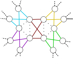
Figure 1. Local representation of $\mathcal{L}^{(2)}_{red}(G)$ using colors to represent the reduced cliques $\mathbb{X}_{i}$. Dashed lines represent edges leading to the remaining parts of the graph. Dotted lines represent the removed triangles.

The next step will be a manipulation of the edges of $\mathcal{L}^{(2)}_{red}(G)$. To this end, we assign labels in $\{0,1\}$ to all edges, where $0$ means closed and $1$ means open, in accordance with classical notations in percolation theory. We apply the following rule.

Definition 2.3.

For the graph $\mathcal{L}^{(2)}_{red}(G)$ assign to the edges in every reduced clique $\mathbb{X}_{i}$ labels in $\{0,1\}$ such that every vertex in $\mathbb{X}_{i}$ is incident in $\mathbb{X}_{i}$ to exactly one edge which has a label $0$ and one which has label $1$. We denote the resulting graph by $\tilde{\mathcal{L}}^{(2)}_{red}(G)$ and the set of open edges (label $1$) in $\tilde{\mathcal{L}}^{(2)}_{red}(G)$ by $\tilde{\mathcal{E}}^{(2)}_{open}$.

Note that there are effectively two choices of labels for any reduced clique $\mathbb{X}_{i}$ and a vertex $v\in\tilde{\mathcal{L}}^{(2)}_{red}(G)$ is incident to exactly two open and two closed edges in $\tilde{\mathcal{L}}^{(2)}_{red}(G)$ since it belongs to exactly two reduced cliques. Remark also, that we can see $\tilde{\mathcal{E}}^{(2)}_{open}$ as a subset of the edge set of $\mathcal{L}^{(2)}_{red}(G)$ when we, again, drop the labels. With a little abuse of notation, we write in both cases $\tilde{\mathcal{E}}^{(2)}_{open}$.

Lemma 2.4.

The edge-induced subgraph of $\mathcal{L}^{(2)}_{red}(G)$ on $\tilde{\mathcal{E}}^{(2)}_{open}$ is a disjoint union of cycles.

Proof.

Any vertex in the edge-induced subgraph has degree $2$ independently of the choice of labels. Consequently, any connected component of the edge-induced subgraph is a simple graph with vertices of valency $2$. Therefore, any connected component is a cycle. Disjointness follows as well. ∎

The edge-induced subgraph will play a central role and its cycles will in the end after applying a set of transformations projected to $G$ to obtain a double cycle cover. In Figure 2 a local representation of the situation is illustrated.

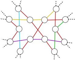
Figure 2. Local representation of $\tilde{\mathcal{L}}^{(2)}_{red}(G)$ using colors to represent the closed edges and the open edges inducing cycles. Closed edges are dark red and open edges are the remaining colors. Open edges of identical color belong to the same cycle.

In fact, working combinatorically through all valid labels of the reduced cliques is unfeasible since there are $2^{|E|}$ possibilities. It is more interesting to look globally at the cycles which a valid labeling implies on $\mathcal{L}^{(2)}_{red}(G)$

Notation 2.5.

Let $\Lambda$ any valid labeling of $\mathcal{L}^{(2)}_{red}(G)$ in the sense of Definition 2.3. We denote by $\Gamma_{\Lambda}$ the set of disjoint cycles resulting from Lemma 2.4. A cycle will be denoted by $\gamma\in\Gamma_{\Lambda}$.

Given any valid labeling $\Lambda$ we can make a link to the line graph of $G$ via a projection, which assigns to any edge in $\mathcal{L}(G)$ a color and two edges have the same color if and only if the corresponding vertices in $\mathcal{L}^{(2)}_{red}(G)$ belong to the same $\gamma\in\Gamma_{\Lambda}$.

Notation 2.6.

We denote the projection from $\Gamma_{\Lambda}$ to $\mathcal{L}(G)$ by $\chi_{\mathcal{E}}$ and the lift from an edge-coloring of $\mathcal{L}(G)$ to some $\Gamma_{\Lambda^{\prime}}$ by $\chi_{\mathcal{E}}^{-1}$.

To make the map well-defined, we have to restrict the colorings of trails in $\mathcal{L}(G)$ since not all give a valid labeling of $\mathcal{L}^{(2)}_{red}(G)$. We take into consideration certain colorings of trails in $\mathcal{L}(G)$, which induce valid cycle double covers of $G$

Definition 2.7.

Let $\tau$ be a set of trails in $\mathcal{L}(G)$ such that all vertices of $\mathcal{L}(G)$ are contained in some trail in $\tau$. Denote by $\Delta=\{\Delta_{1},\Delta_{2},\Delta_{3}\}$ a triangle in $\mathcal{L}(G)$, which is induced by a single vertex in $G$ (see [Har72]). Denote the remaining two neighbors of $\Delta_{1}$ by $v_{1}$ and $v_{2}$. We say $\tau$ is valid if for all trails $\phi\in\tau$ and $\Delta_{1}\in\phi$ as well as $\langle\Delta_{1},\Delta_{2}\rangle,\langle\Delta_{1},\Delta_{3}\rangle$ implies $\langle\Delta_{1},v_{1}\rangle,\langle\Delta_{1},v_{2}\rangle\in\phi$.

We will from now on only consider valid colorings in the sense of Definition 2.7. Each valid labeling can now projected to $G$ as shown in Figure 3, where $\pi_{\mathrm{chrom}}$ assigns to any edge in $G$ one or two colors, corresponding to the colors of the edges incident to the corresponding vertex in $\mathcal{L}(G)$.

Figure 3. The construction and, then, projection of the labeled reduced double line graph first to a spanning set of trails $\tau_{\mathcal{L}(G)}$ in $\mathcal{L}(G)$ and, then, to a set of closed walks $\omega_{G}$ in $G$ such that the union over all walks traverses every edge exactly twice.

We fix one important property in the following observation, which follows directly from the construction as mentioned in Figure 3.

Observation 2.8.

The set $\omega_{G}$ resulting from the projection of the set of disjoint cycles in $\mathcal{L}^{(2)}_{red}(G)$ spanned by $\tilde{\mathcal{E}}^{(2)}_{open}$ is a set of closed walks such that the union over all walks traverses every edge exactly twice.

It turns out that it is not necessary, to consider all possibilities since only a few labels are really of interest modulo a set of label transformations. Those are exactly given by the labels which are projected under $\pi\circ\chi_{\mathcal{E}}$ to a set of cycles in $G$. They have a specific structure which we define in the next Subsection and show also their existence in the case of bridgeless cubic graphs.

2.2. Type A and Type B self-intersections

This subsection will develop the cycles induced by $\tilde{\mathcal{E}}^{(2)}_{open}$ on $\mathcal{L}^{(2)}_{red}(G)$ as the main tool. For this, we need a few notations and definitions. They should render the construction more accessible since they lift everything to the space of induced cycles and we can drop the explicit reference to $\mathcal{L}^{(2)}_{red}(G)$ and $\tilde{\mathcal{L}}^{(2)}_{red}(G)$. We have to establish a structural property defining adjacent cycles in $\tilde{\mathcal{L}}^{(2)}_{red}(G)$ before coming back to the link between $\mathcal{L}(G)$ and $\tilde{\mathcal{L}}^{(2)}_{red}(G)$.

Definition 2.9.

Let $\gamma_{1},\gamma_{2}\in\Gamma_{\Lambda}$. If there is a reduced clique $\mathbb{X}$ and edges $e_{1}\in\gamma_{1}$, $e_{2}\in\gamma_{2}$ such that $e_{1},e_{2}\in\mathbb{X}$, then we call $\gamma_{1},\gamma_{2}$ adjacent. Additionally, we say that $\mathbb{X}$ joins $\gamma_{1}$ and $\gamma_{2}$.

Note that a reduced clique joining two cycles is not necessarily unique. Adjacency can locally be understood as illustrated in Figure 4. If two cycles are adjacent, the layout in Figure 4 can naturally be transformed to the diagonals being open.

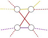
Figure 4. Two adjacent cycles and a joining reduced clique. Red edges are again closed and cycles are yellow and purple.

Nonetheless, for illustration purposes, we will use the layout presented in Figure 4 as an idea for adjacent cycles while the diagonals will be employed for self-intersections as defined in Definition 2.10.

Definition 2.10.

Let $\gamma\in\Gamma_{\Lambda}$. If there is a reduced clique $\mathbb{X}$ such that both open edges in $\mathbb{X}$ belong to $\gamma$, then we say that $\gamma$ has a self-intersection and $\mathbb{X}$ is a self-intersection of $\gamma$.

Again, self-intersections are not necessarily unique. A possible illustration shown in Figure 5 serves, again, as an idea or intuition. In particular, self-intersections will play a crucial role in the proof in Section 3 since they will arise from cycle cover choices which traverse the same edge in $G$ twice.

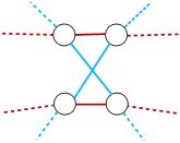
Figure 5. A self-intersection $\mathbb{X}$ of some cycle $\gamma$. The cycle $\gamma$ is colored in light blue.

The distinction between adjacency and self-intersections is a binary property of reduced cliques. Moreover, self-intersections of any cycle $\gamma$ can, again, be differentiated into two topologically different types. For this, we need the following cycle notation, which is inspired by knot theory.

Notation 2.11.

We will use a mesoscopic perspective on cycles in what follows, which requires a set of diagrams.

1. A simple cycle without any additional structural conditions:

   

2. A simple cycle without any self-intersections:

   

3. Two adjacent cycles joined by some reduced clique:

   

4. A self-intersecting cycle with focus on a self-intersection $\mathbb{X}$ called Type A:

   

5. A self-intersecting cycle with focus on a self-intersection $\mathbb{X}$ called Type B:

   

We want to emphasize that ”intersections” in the sense of Definition 2.10 and as presented in Notation 2.11 d) and e) are not actual intersections which traverse a vertex or an edge twice. It is solely a view on the structure of the reduced cliques $\mathbb{X}_{i}$.

Definition 2.12.

Consider a valid labeling $\Lambda$ and the associated $\tilde{\mathcal{L}}^{(2)}_{red}(G)$. For $\mathbb{X}$ a reduced clique in $\tilde{\mathcal{L}}^{(2)}_{red}(G)$, we call $\mathcal{F}_{\mathbb{X}}$ mapping every label $x$ of edges in $\mathbb{X}$ to $1-x$ a label inversion. We write, with a little abuse of notation $\mathcal{F}_{\mathbb{X}}(\tilde{\mathcal{L}}^{(2)}_{red}(G))$ if we talk about the structure change in the whole graph after the change of the labels in $\mathbb{X}$ and $\mathcal{F}_{\mathbb{X}}(\mathbb{X})$, when we only consider the local changes.

Label inversions can be seen in many different ways, from generators of spin dynamics in statistical mechanics to open-closed path flippings in electrical networks and combined with their underlying reduced cycle $\mathbb{X}$ they even can be interpreted as inversions in logic gates with two inputs and two outputs. Label inversions have the following important properties.

Observation 2.13.

Let $\mathbb{X}$ be a reduced clique. Then, we have the following properties.

1. If $\mathbb{X}$ joins two adjacent cycles, then $\mathcal{F}_{\mathbb{X}}(\mathbb{X})$ is an intersection of Type B.

2. If $\mathbb{X}$ is an intersection of Type B, then $\mathcal{F}_{\mathbb{X}}(\mathbb{X})$ joins two adjacent cycles.

3. If $\mathbb{X}$ is an intersection of Type A, then $\mathcal{F}_{\mathbb{X}}(\mathbb{X})$ is an intersection of Type A.

These can be checked or seen directly from the Notation 2.11 and associated diagrams, and form the basis for further arguments and more involved constructions joining and separating cycles. The goal of the whole effort is demonstrated in the following Lemma.

Lemma 2.14.

Let $\Lambda$ a set of labels such that there are no self-intersections in $\tilde{\mathcal{L}}^{(2)}_{red}(G)$. Then, the projection of $\Lambda$ to $G$ under $\pi_{\mathrm{chrom}}\circ\chi_{\mathcal{E}}$ is a set of cycles.

Proof.

Assume that $\pi_{\mathrm{chrom}}\circ\chi_{\mathcal{E}}(\Lambda)$ implies a closed walk on $G$, which is not a cycle and which, therefore, traverses and edge twice. The inverse operation would imply that there is a vertex in $\mathcal{L}(G)$ such that all incident edges have the same color. This is impossible by assumption on $\Lambda$ since the lift of this vertex would give a self-intersection in $\tilde{\mathcal{L}}^{(2)}_{red}(G)$. ∎

Our goal is, therefore, to find a set of labels $\Lambda$, which has no self-intersections. To avoid lengthy wordings in what follows, we use the following definition.

Definition 2.15.

Let $\mathbb{X}$ be an intersection of Type A or B. We call $\mathbb{X}$ reducible, if there is a finite number of label inversions $\mathcal{F}_{\mathbb{X}_{1}},\ldots,\mathcal{F}_{\mathbb{X}_{n}}$ such that $\mathbb{X}$ joins two cycles in $\mathcal{F}_{\mathbb{X}_{1}}\circ\ldots\circ\mathcal{F}_{\mathbb{X}_{n}}(\tilde{\mathcal{L}}^{(2)}_{red}(G))$. In any other case, we call $\mathbb{X}$ irreducible.

Indeed, by Observation 2.13 all intersections of Type B are reducible, using simply their assigned label transformation $\mathcal{F}_{\mathbb{X}}$. This is not always the case for Type A intersections. The first case, for which reducibility fails, will be discussed next.

Lemma 2.16.

Let $G$ be a simple connected cubic graph. If $G$ has a bridge, then for all valid labelings $\Lambda$ there is a self-intersection $\mathbb{X}$ of Type A in $\tilde{\mathcal{L}}^{(2)}_{red}(G)$.

Proof.

A bridge in $G$ is a cut-vertex in $\mathcal{L}(G)$ and vice-versa. Call this vertex in $\mathcal{L}(G)$ simply $q$. Then, the vertex $q$ implies by construction a reduced clique in $\tilde{\mathcal{L}}^{(2)}_{red}(G)$, which we call $\mathbb{X}_{q}$. Since any trail in $\mathcal{L}(G)$ containing $q$ has to go through $q$ twice, the lift to $\mathbb{X}_{q}$ implies a Type A self-intersection which cannot be resolved since it separates the cycle into two independent parts which cannot be joined otherwise. ∎

The obvious consequence is that said Type A intersection is irreducible and it is, therefore, impossible to obtain labelings without self-intersections if the underlying graph $G$ has a bridge. The statement in Lemma 2.16 is, indeed, an equivalence but the second part, stated in Proposition 2.17, needs further work which we need to do first.

Proposition 2.17.

Let $G$ be a simple connected cubic graph. If for all valid labelings $\Lambda$ there is a self-intersection $\mathbb{X}$ of Type A in $\tilde{\mathcal{L}}^{(2)}_{red}(G)$, then $G$ has a bridge.

We have to postpone the proof, which will be done constructively, based on the following results. For parts of it we need to take a more global perspective on the cycles than what we have done so far. In particular, we develop the adjacency relationship of cycles, which could be further developed as the graph of cycles as a function of the labels.

Definition 2.18.

Let $\gamma_{1},\gamma_{2}\in\Gamma_{\Lambda}$ be non-adjacent cycles. We say that a cycle $\gamma_{3}$ joins $\gamma_{1}$ and $\gamma_{2}$, if $\gamma_{3}$ is adjacent to both $\gamma_{1}$ and $\gamma_{2}$.

It turns out, that two fixed cycles can always be joined as explain in the following Observation 2.19.

Observation 2.19.

Let $\gamma_{1},\gamma_{2}\in\Gamma_{\Lambda}$ be non-adjacent cycles. Then, there is a finite number of label inversions $\mathcal{F}_{\mathbb{X}_{1}},\ldots,\mathcal{F}_{\mathbb{X}_{n}}$ such that $\gamma_{1},\gamma_{2}$ belong to $\mathcal{F}_{\mathbb{X}_{1}}(\ldots\mathcal{F}_{\mathbb{X}_{n-1}}(\mathcal{F}_{\mathbb{X}_{n}}(\tilde{\mathcal{L}}^{(2)}_{red}(G)))\ldots)$ and $\gamma_{1},\gamma_{2}$ are joined by some cycle $\gamma_{3}$.

Observation 2.19 can be interpreted on a higher level as the connectedness of the graph defined by all possible cycles over all valid labelings with adjacency given by Definition 2.9.

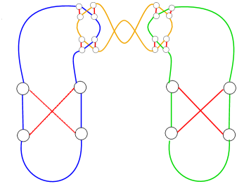
Figure 6. Cycles $\mathbb{X}_{1},\mathbb{X}_{2}$ containing Type A self-intersections with joining cycle potentially obtained by some label inversions $\mathbb{F}$.

The final preparation step consists in capturing the possible positions of Type A self-intersection. To this end, we employ vertex-cuts in $\mathcal{L}(G)$ which we lift to $\tilde{\mathcal{L}}_{red}^{(2)}(G)$, which follows directly from the structure of the line graph of a cubic bridgeless graph.

Definition 2.20.

Let $v\in\mathcal{L}(G)$. Then, we we define a minimal vertex-cut $\mathbb{V}_{v}$ centered at $v$ as a vertex-cut in $\mathcal{L}(G)$ with $v\in\mathbb{V}_{v}$, for all $v^{\prime}\in\mathbb{V}_{v}$ the set $\mathbb{V}_{v}\backslash\{v^{\prime}\}$ is not a vertex-cut and $|\mathbb{V}_{v}|$ is minimal over all such sets.

We discuss the implications and results of Definition 2.20 in Appendix A. Evidently, this concept can be lifted to $\tilde{\mathcal{L}}_{red}^{(2)}(G)$ by first identifying the edge $e$ in $G$ with a vertex $v_{e}$ in $\mathcal{L}(G)$ and then associating a reduced clique $\mathbb{X}_{v}$ to $v_{e}$. To this end, we employ the perspective of the line-graph operator discussed in [Har72] based on replacement of each vertex with a complete graph of size $4$ and edge contraction of the old edges.

2.3. Proof of Proposition 2.17

We recommend that the reader first goes through Appendix A to familiarize themselves with the concepts around lifted minimal centered vertex-cuts and minimal centered vertex-cuts in the line graph. We use them extensively in the proof.

Proof of Proposition 2.17.

For this proof, we employ centered vertex-cuts in $\mathcal{L}(G)$ as the central tool and assume that $G$ is bridge-free. The goal is to show that under these conditions any Type A self-intersection can be reduced by label transformations which do not create new Type A self-intersections. This gives a strongly monotonous sequence of the number of Type A self-intersections which by construction converges to $0$.

2.3.1. Constructive reducibility of Type A self-intersections

To illustrate, we consider first the case that there is a valid labeling such that all open edges are traversed by the same cycle. Pick any Type A self-intersection $\mathbb{X}$. Then the cycle is separated by $\mathbb{X}$ into an ”upper” part and a ”lower” part, which are joined by at least one other self-intersection $\mathbb{X}^{\prime}$. Inverting the labels of both self-intersections separates this cycle into two cycles and $\mathbb{X}$ as wellas $\mathbb{X}^{\prime}$ join the two. The general idea in what follows will be along the same lines. We look for a way to join the ”upper” and ”lower” part of the cycle containing some Type A self-intersection $\mathbb{X}$ and invert the necessary labels. Finally, we have to show that this does not create Type A self-intersections, which leads to a strictly monotonous process converging to $0$. This will be done in Section 2.3.2.

Figure 7. Proof sketch of Proposition 2.17 based on reduction of type A self-intersection

From this point on we can, due to the previous discussion, assume that there are at least two cycles induced by the open edges in $\mathcal{L}^{(2)}_{red}$. Pick any Type A self-intersection $\mathbb{X}$ in $\tilde{\mathcal{L}}_{red}^{(2)}(G)$ and associate it to a vertex in $v\in\mathcal{L}(G)$ as discussed in [Har72]. We put the emphasis on this link by changing the name of $\mathbb{X}$ to $\mathbb{X}_{v}$. Denote by $\mathbb{V}_{v}$ a minimal vertex cut in $\mathcal{L}(G)$ centered at $v$ and by $\mathcal{V}_{\mathbb{X}}$ the associated reduced cliques in $\tilde{\mathcal{L}}_{red}^{(2)}(G)$. Note that necessarily by construction $\mathbb{X}\in\mathcal{V}_{\mathbb{X}}$ which is already suggested by the notation. We now go through all possible forms in which minimal vertex cuts may occur as discussed in Appendix A. From Appendix A and Observation 2.19 we can conclude that in any of the two connected components cycles going through the lifted vertex cut are either adjacent or are joined by a cycle which lies completely in said connected component. The remainder of the proof is constructive/illustrative and based on the following catalog of lifted vertex cut structures. They are ordered by the size of the vertex cut $\mathbb{V}_{v}$. For every case but the case $|\mathbb{V}_{v}|=2$ the number of cases is given by the partition function of $|\mathbb{V}_{v}|$. We start with the case $|\mathbb{V}_{v}|=2$.

Figure 8. All possible situations for vertex cuts $\mathbb{V}_{v}$ with $|\mathbb{V}_{v}|=2$. See Appendix A for the case of both cut vertices being neighbors in $\mathcal{L}(G)$.

We continue with the case $|\mathbb{V}_{v}|=3$.

(a)

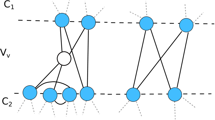
(b)

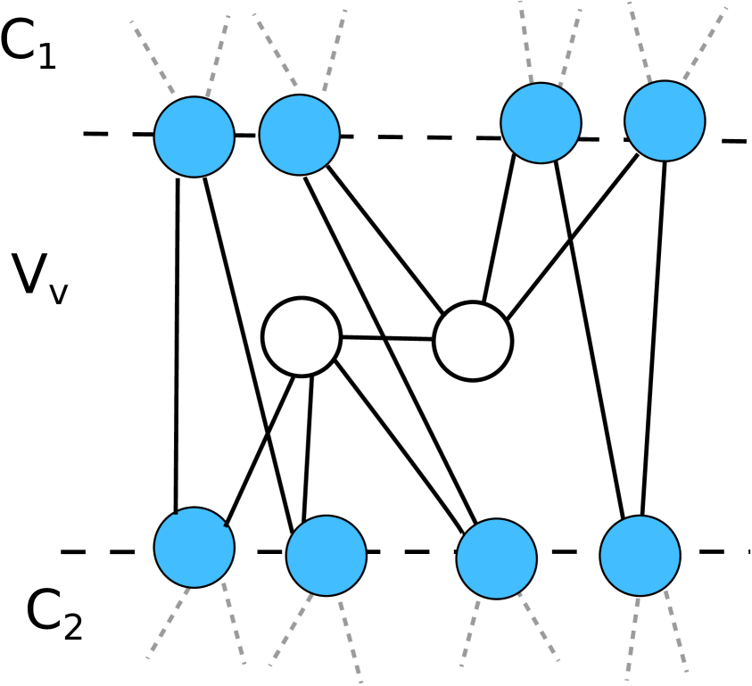
(c)

Figure 9. All possible situations for vertex cuts $\mathbb{V}_{v}$ with $|\mathbb{V}_{v}|=3$.

Finally, the case $|\mathbb{V}_{v}|=4$.

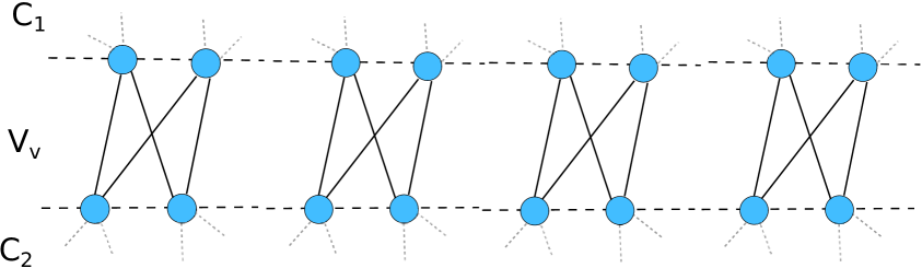
(a)

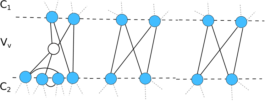
(b)

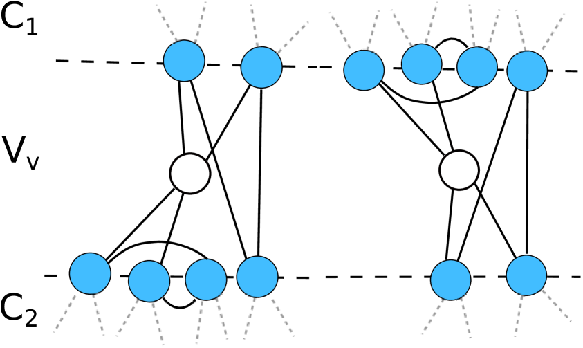
(c)

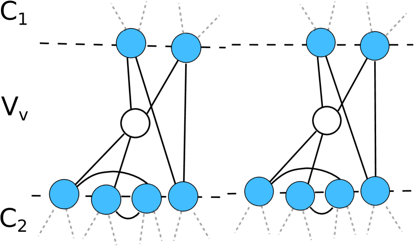
(d)

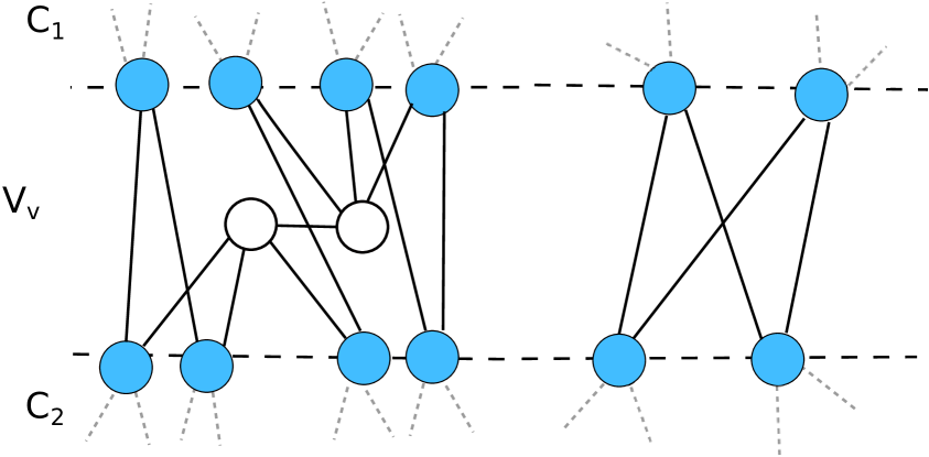
(e)

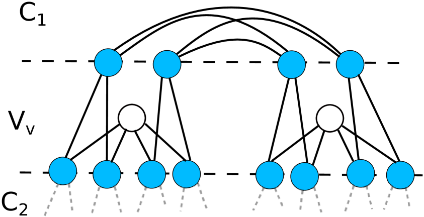
(f)

Figure 10. All possible situations for vertex cuts $\mathbb{V}_{v}$ with $|\mathbb{V}_{v}|=4$.

Note that we will only consider the situation shown in Figure 10(f) by construction. The remaining cases carry, nonetheless, interesting topological properties but do not contribute to our goal, so they will most likely content of further research. This reduces in what follows the number of cases tremendously.

Generic cycles associated to lifted vertex cuts: A generic cycle denotes simply the situation that any set of labels $\Lambda$ induces a set of cycles in $\mathcal{L}^{(2)}_{red}$. So, even without a specific set of labels given, we can think about the cycle behavior in the two lifted connected components $\mathcal{C}_{1}$ and $\mathcal{C}_{2}$ as well as their traversal of the lifted centered vertex cut $\mathcal{V}_{\mathbb{X}_{v}}$ The following generic cycles can be associated to the corresponding vertex cuts. This is a combinatorial exercise where symmetric situations with respect to the structure of the cycles are identified.

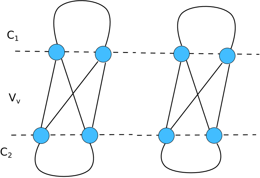
(a)

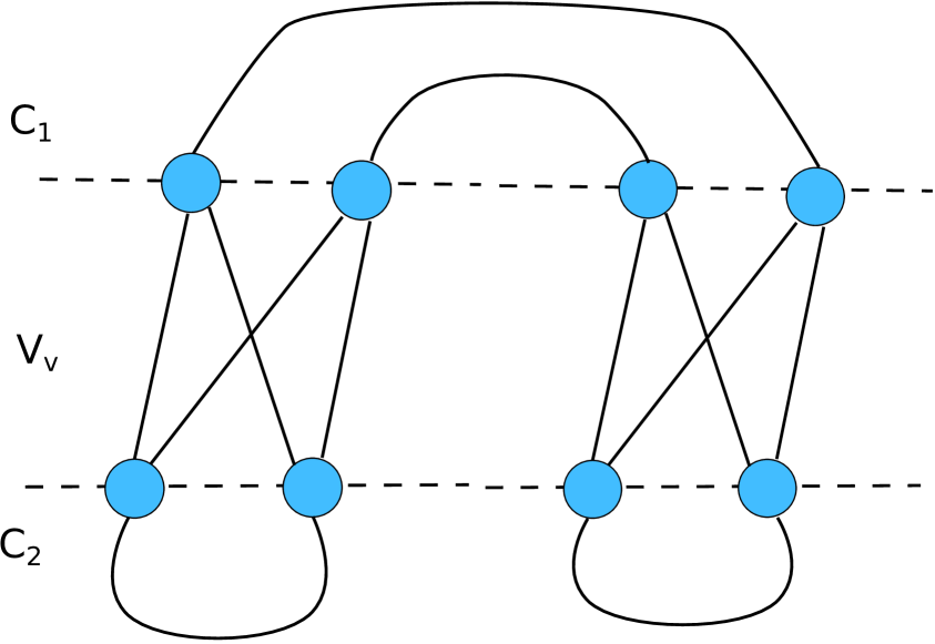
(b)

Figure 11. All possible generic cycles for vertex cuts $\mathbb{V}_{v}$ with $|\mathbb{V}_{v}|=2$ based on Figure 8.

The following sub-cases arise under generic cycle representations. We go from Figure 8 to Figure 10(f) through all relevant cases and their implied generic cycles.

(a)

(b)

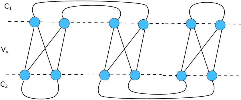
(c)

(d)

(e)

(f)

Figure 12. All possible generic cycles for vertex cuts $\mathbb{V}_{v}$ with $|\mathbb{V}_{v}|=3$ based on Figure 9(a).

(a)

(b)

(c)

(d)

(e)

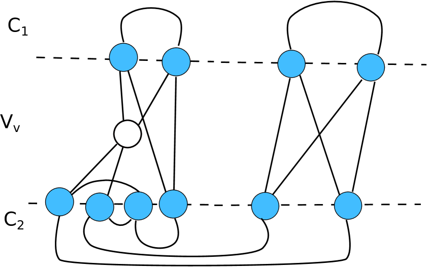
(f)

Figure 13. All possible generic cycles for vertex cuts $\mathbb{V}_{v}$ with $|\mathbb{V}_{v}|=3$ based on Figure 9(b).

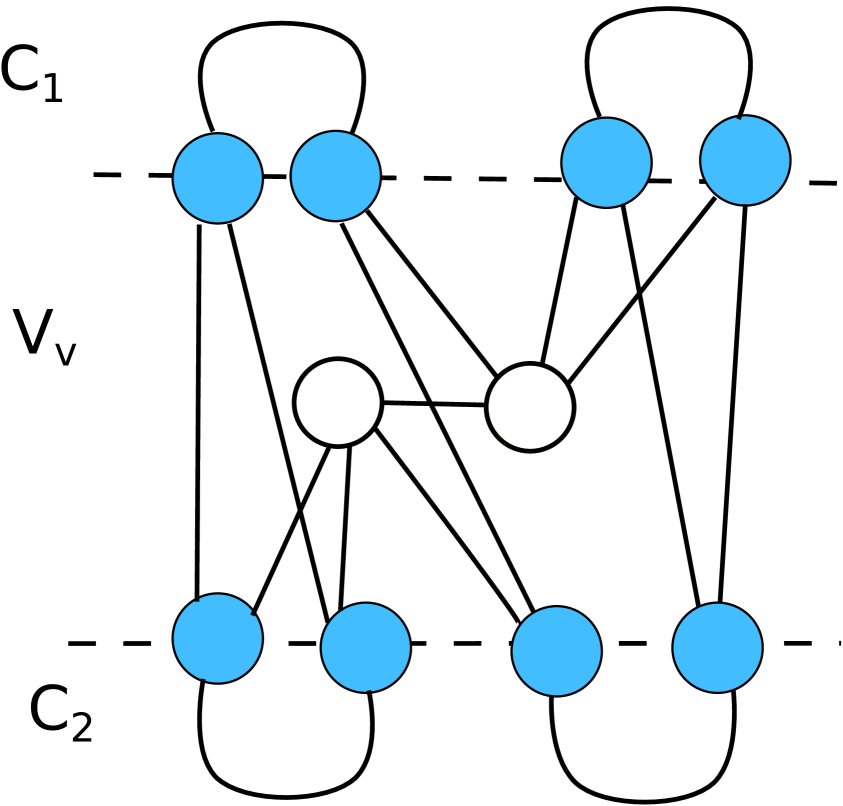
(a)

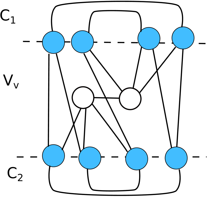
(b)

(c)

(d)

(e)

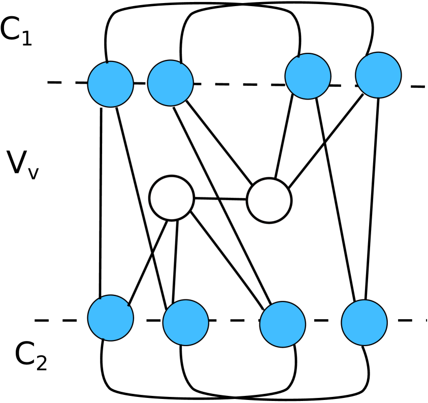
(f)

Figure 14. All possible generic cycles for vertex cuts $\mathbb{V}_{v}$ with $|\mathbb{V}_{v}|=3$ based on Figure 29(b).

(a)

(b)

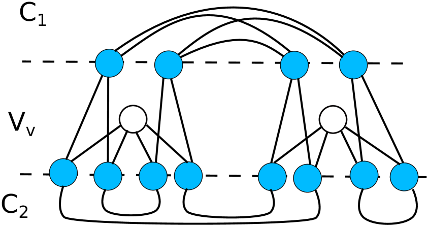
(c)

Figure 15. All possible generic cycles for vertex cuts $\mathbb{V}_{v}$ with $|\mathbb{V}_{v}|=4$ based on Figure 10(f).

Having listed all cases up to symmetry of generic cycles, we approach now the reduction of the Type A self-intersections. We employ the intuition developed at the beginning of the proof to connect the ”upper” part and ”lower” part of the cycle containing the Type A self-intersection which we want to reduce. This will, again be a catalog of all cases modulo symmetries. In the left column we present the case containing Type A self-intersections and in the right column the resolved variant except for the case where all self-intersections in the lifted centered vertex cut are Type B. We then show only a resolved version.

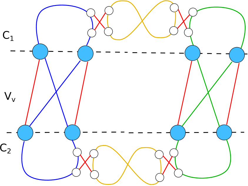
(a)

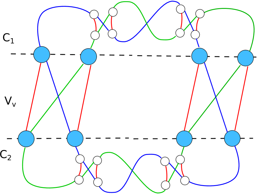
(b)

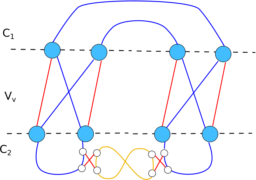
(c)

(d)

Figure 16. Resolutions of Figure 11.

The method we presented in Figure 16 using Type B self-intersections and flips of the former type A self-intersections to reduce the present type A self-intersection via intermediary cycles in the lift of $C_{1}$ and $C_{2}$, whose existence is assured by Observation 2.19, will be the general method in all other cases. Note that adjacency of the two cycles crossing the lift of the centered vertex cut is also contained in this view, using an ”empty” intermediary cycle. We move on to the first case of the size $3$ centered vertex cut as presented in Figure 12. Note that the all cases in Figure 12 can be resolved as is done in Figure 16 no matter which reduced clique in the lift of $\mathbb{V}_{v}$ is considered to be the lift of $v$. The existence of the necessary cycles in the lifts of $C_{1}$ and $C_{2}$, which might, again, be, potentially, empty, is assured by Observation 2.19 and the fact that traversals between the lifts of $C_{1}$ and $C_{2}$ are only possible through the lift of the centered vertex cut. But the traversals are fixed. Therefore, we can consider the cases in Figure 12 as resolved. We continue with the discussion of the cases shown in Figure 13. We want to emphasize, that sometimes Type A self-intersections are still present in the designs, which would then be reduced by another iteration of the same construction. But no new ones are created. We work on that claim in detail in Subsection 2.3.2.

(a)

(b)

(c)

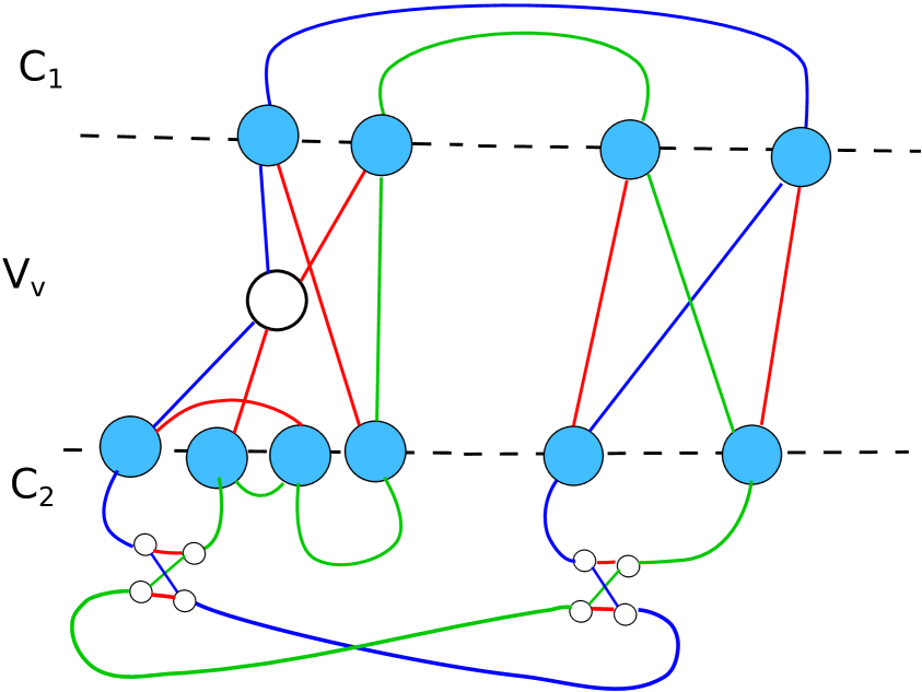
(d)

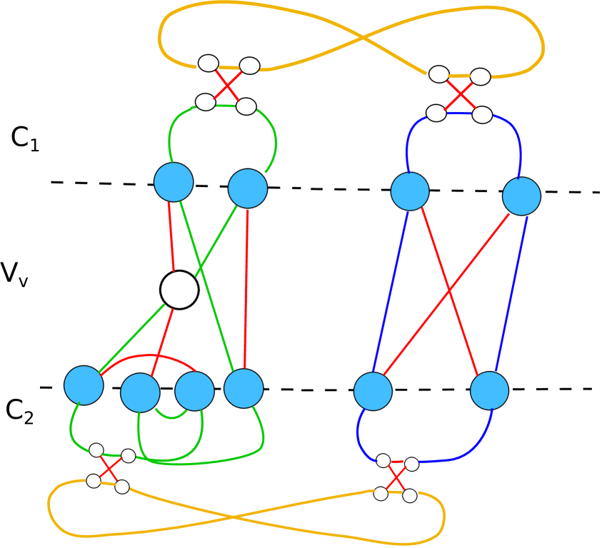
(e)

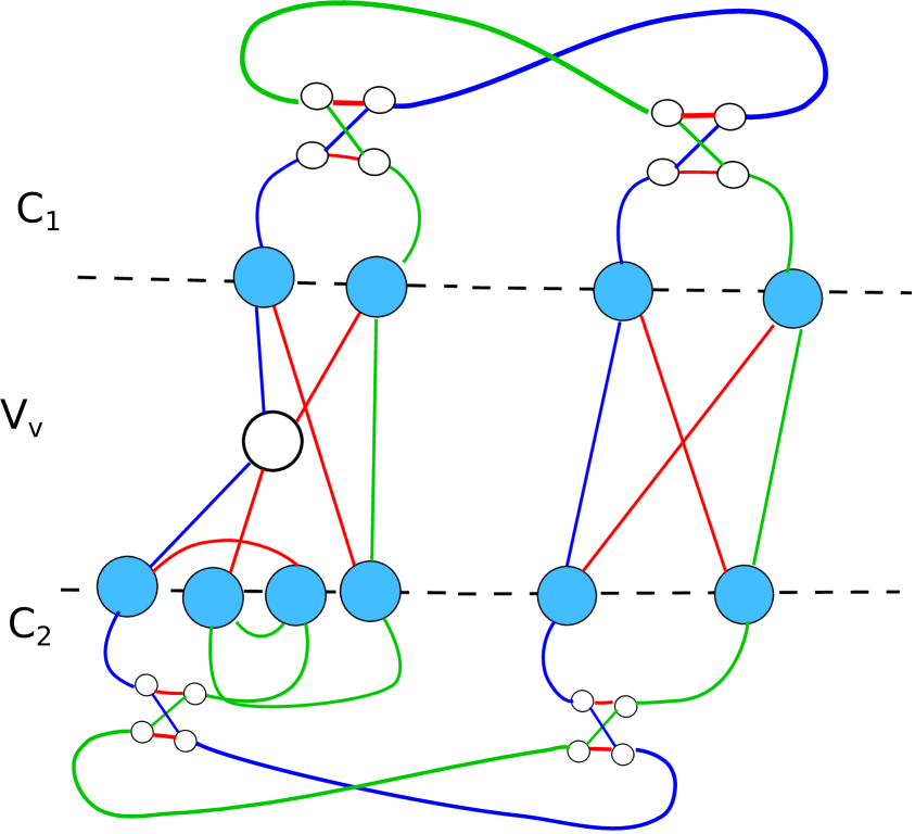
(f)

Figure 17. Resolutions of Figures 13(a) to 13(c).

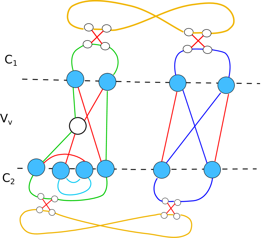
(a)

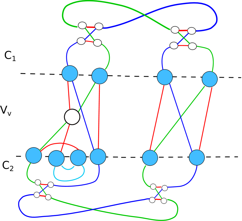
(b)

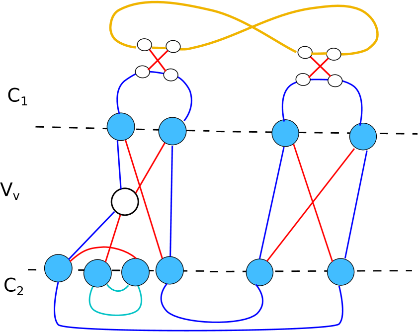
(c)

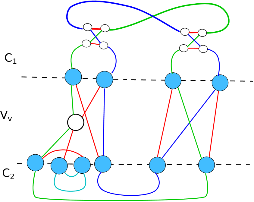
(d)

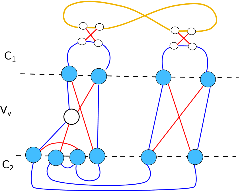
(e)

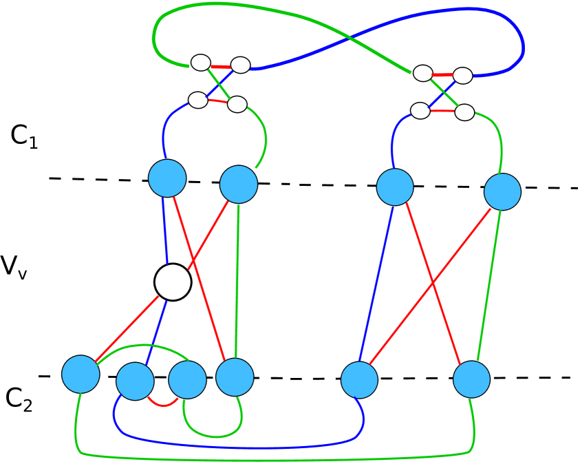
(f)

Figure 18. Resolutions of Figures 13(d) to 13(f).

The next step will focus on the cases shown in Figure 14.

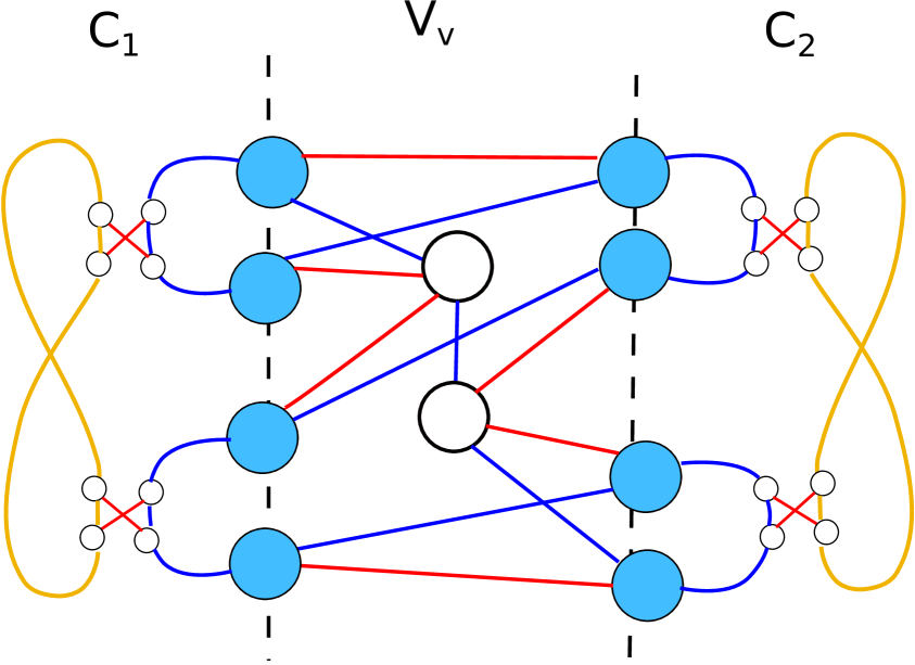
(a)

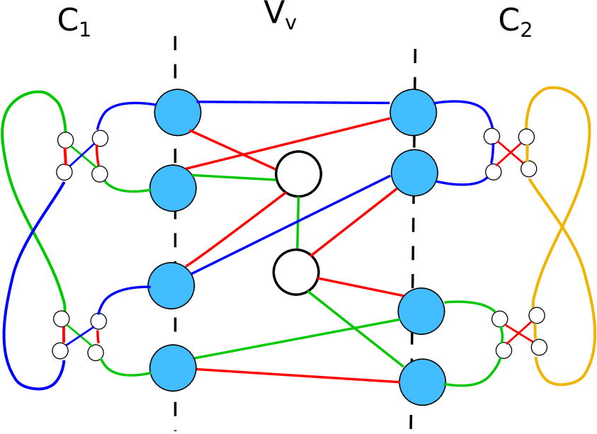
(b)

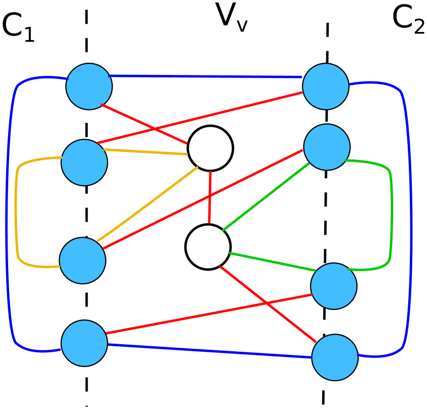
(c)

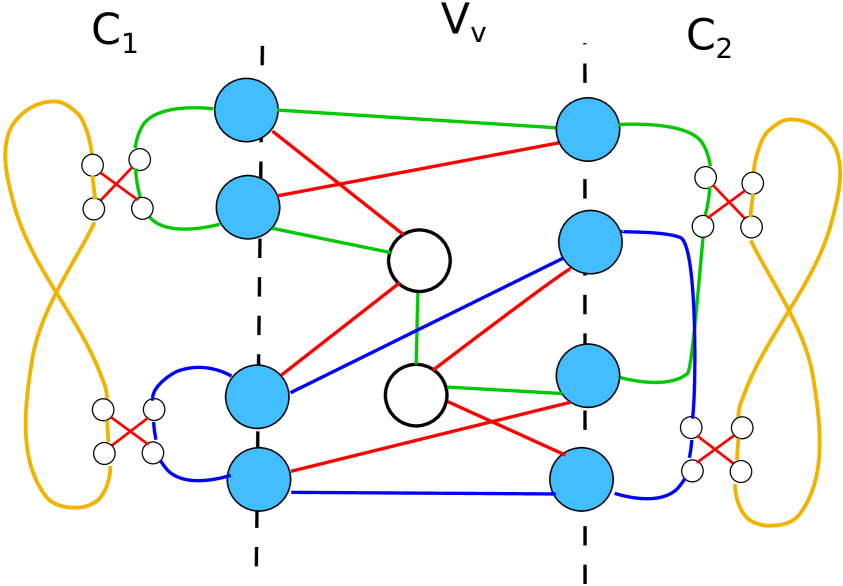
(d)

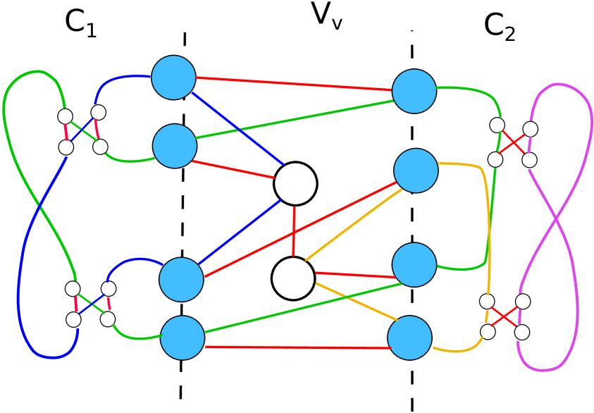
(e)

Figure 19. Resolutions of Figures 14(a) to 14(c). Some are turned by 90° for aesthetic reasons. Note that in Figure 19(c) there is a labeling within the lifted vertex cut such that any self-intersection separate into independent cycles.

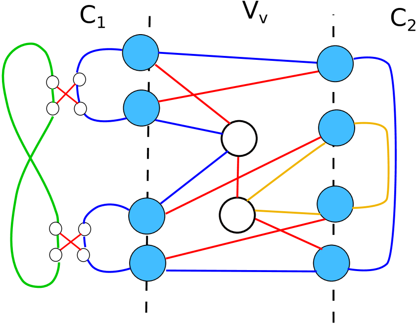
(a)

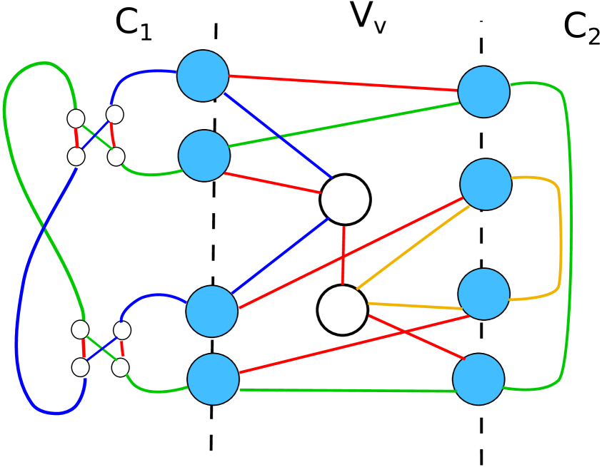
(b)

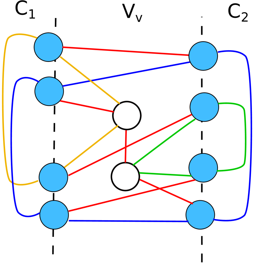
(c)

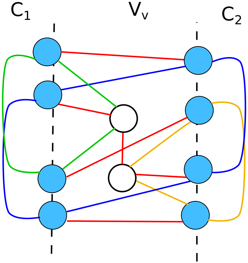
(d)

Figure 20. Resolutions of Figures 14(d) to 14(f). Also in Figures 20(c) and 20(d) there is a labeling within the lifted vertex cut such that any self-intersection separate into independent cycles.

We conclude the entire discussion with considerations in Figure 15.

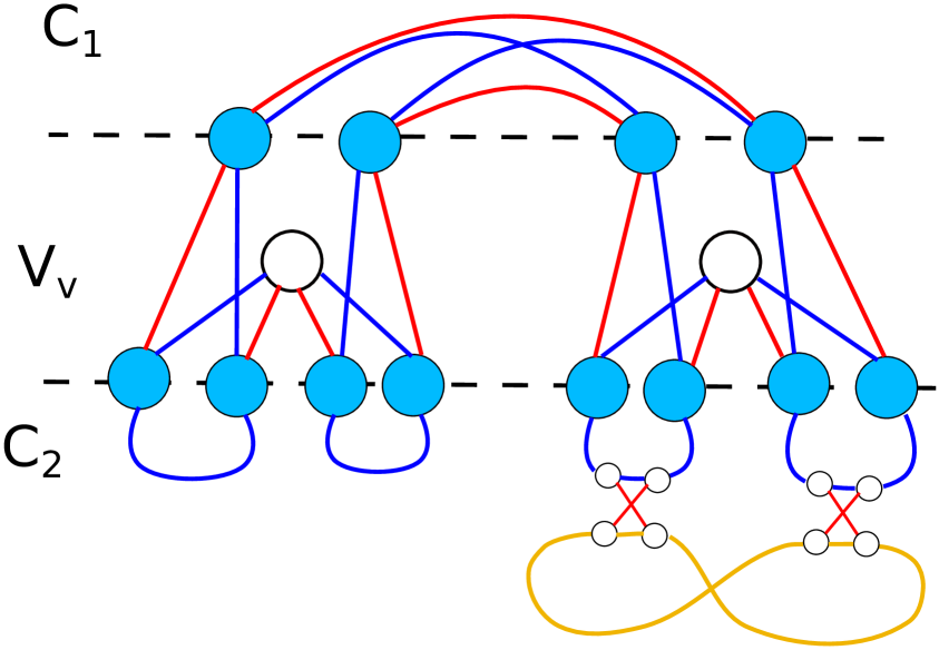
(a)

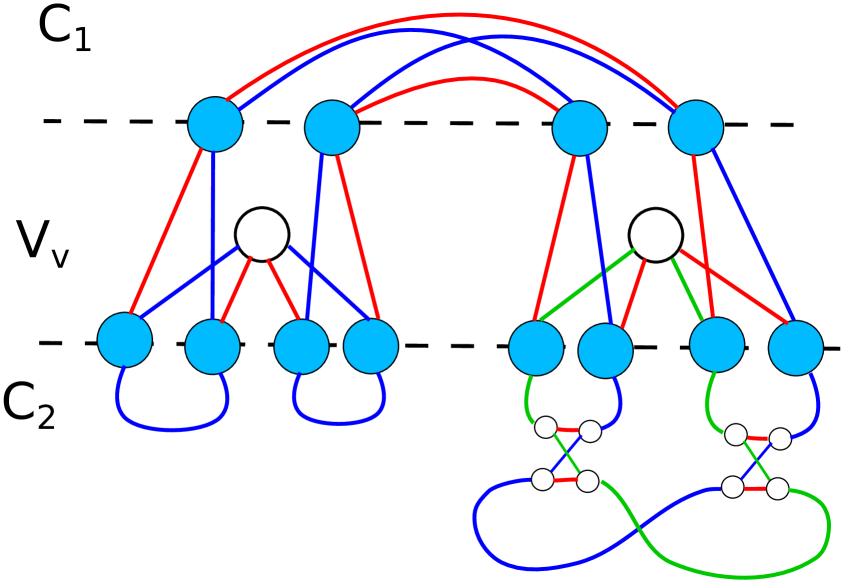
(b)

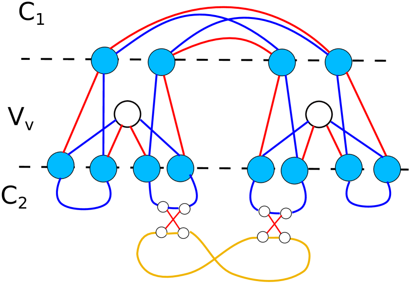
(c)

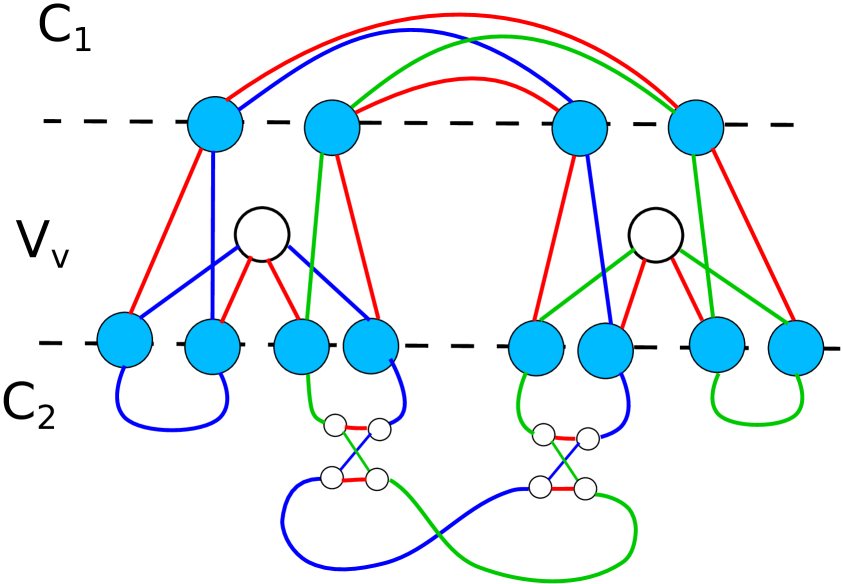
(d)

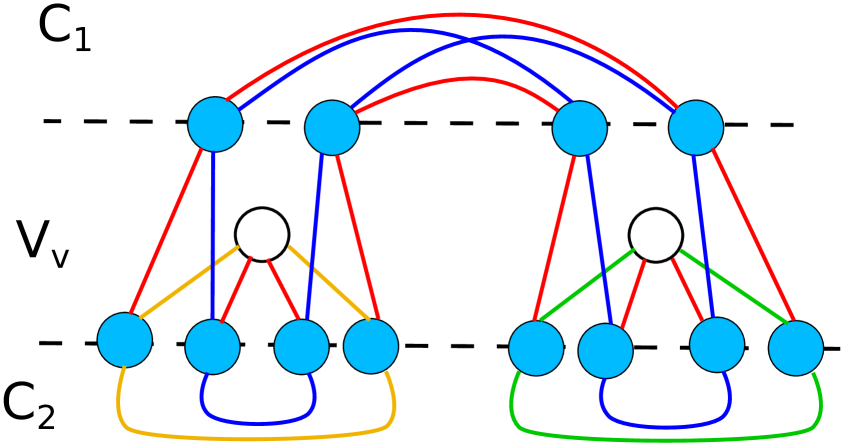
(e)

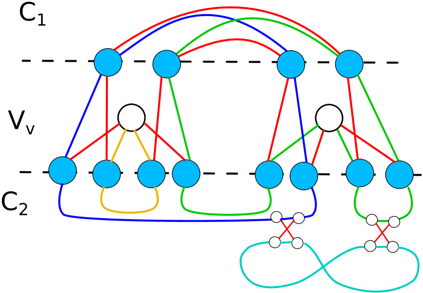
(f)

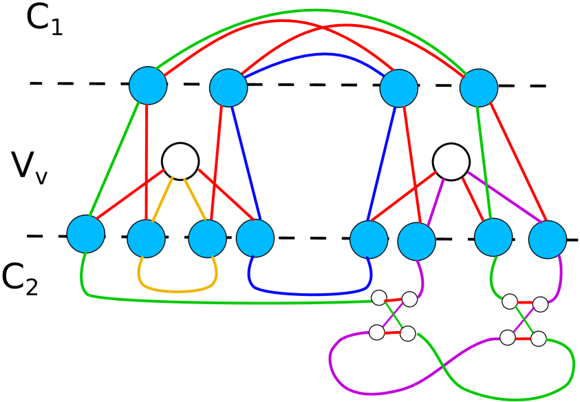
(g)

Figure 21. Resolutions of Figure 15. Note that in Figure 21(e) any self-intersection within the lifted vertex cut is of Type B independently of the label structure in the lifted vertex cut. Figures 21(b) and 21(d) can be completely reduced, i.e., no more Type A self-intersections, by applying the same construction again.

This concludes the list of cases which may arise for Type A self-intersections under the conditions of Proposition 2.17 and the assumption that a bridge exists. In all cases, we can reduce the present Type A self-intersections. Next we show that no are created in the process.

2.3.2. Monotonicity of number of Type A self-intersections

So far, we have been occupied with the question of removing Type A intersections. Naturally, we also need to know if and how they might be created, pushing us away from the desired state where no Type A intersections are present. In particular, reducibility of one reduced clique is not sufficient to ensure that no Type A intersections are created by the associated vector of label inversions. We are in particular interested in the cases from Observation 2.19 and the resolution of Type A self-intersections as discussed in the previous subsection 2.3.1. We illustrate the situation based on Figure 22.

Figure 22. Generic view of a Type A self-intersection where a cycle connects the ”upper” and ”lower” part of the cycle relative to the Type A self-intersection.

In Figure 23 one can see that the process we used beforehand is prone to the creation of self-intersections of Type A if not completely applied. It remains to show, that there is a right way of applying the construction. In fact, this depends fully on the position of the Type B intersections within the merged final cycle before applying label transformations and only the label transformation of the initial Type A self-intersection $\mathbb{X}$, which we want to resolve, decides over the character of the initial Type B self-intersections, like the five shown in Figure 22. This boils down to three cases, a Type B intersection in the same cycle $\gamma$ as the Type A self-intersection which we want to reduce, a Type B intersection in a connecting cycle and, finally, a Type B intersection joining a connecting cycle with the cycle containing the Type A self-intersection which we want to reduce but which is not transformed via a label inversion $\mathcal{F}_{\mathbb{X}}$. The first and second case are directly resolved, since the structure of a Type B intersection is not altered, it can only stay a Type B self-intersection or become a join of two independent cycles. In the third case, there are, again, three possibilities, depending on the number of Type B self-intersections joining the cycle $\gamma$ and connecting cycle $\gamma^{\prime}$. They are shown in Figure 23 and the corresponding resolution without the creation of additional Type A self-intersections in Figure 24.

Figure 23. Type A self-intersection with label inversion and cycle merge giving rise to new Type A self-intersections.

We want to put the emphasis on the light blue cycle in Figure 24, which increases the overall number of cycles and is necessary for the reduction of all self-intersections present in the diagram. Indeed, adding additional joining reduced cliques between $\gamma$ and $\gamma^{\prime}$ boils down to the same case as presented in Figure 23, because all relative pairwise positions of reduced cliques are covered by Figure 23.

Figure 24. Type A self-intersection with label inversion and cycle merge giving rise to new Type A self-intersections.

Therefore, we can always avoid creating Type A self-intersections from Type B self-intersections in any case discussed in Subsection 2.3.1. Consequently, putting together Subsection 2.3.1 and 2.3.2, we can conclude under the assumptions of Proposition 2.17, that there is a sequence $\mathbb{F}=(\mathbb{F}_{l})$ of vectors of label inversions

$$\mathbb{F}_{l}=\mathcal{F}_{X_{i_{n}}}\circ\ldots\circ\mathcal{F}_{X_{i_{1}}}$$

such that the number of Type A self-intersections in $\mathbb{F}_{l}(\mathcal{L}^{(2)}_{red})$ is strictly monotonously decreasing in $l$, integer-valued and non-negative. This implies, that we find on any bridgeless graph a set of labels such that there are no Type A self-intersections in $\mathcal{L}^{(2)}_{red}$. This allows us to conclude the proof of Proposition 2.17. ∎ Having finished the proof of Proposition 2.17, the cycle double cover conjecture can now be proven.

3. Proof of Theorem 1.1

The proof of Theorem 1.1 is fully based on the results concerning the reduced order two line graph $\mathcal{L}^{(2)}_{red}(G)$ with an appropriate binary open-close labeling of the edges. The proof then works as presented in Figure 25.

Figure 25. The proof setup with objects and operators $\mathcal{D}_{\mathcal{T}}$ construction of $\tilde{\mathcal{L}}_{red}^{(2)}(G)$ (Definition 2.3), $\mathbb{T}_{\Lambda}$ set of label inversions (Definition 2.12) encapsulating the construction from Section 2.

Proof of Theorem 1.1.

Under the assumption that $G$ is bridgeless, we obtain from Proposition 2.17 that there is a set of labelings $\Lambda^{\ast}$ of $\mathcal{L}^{(2)}_{red}(G)$ such that the resulting cycles $\Gamma_{\Lambda^{\ast}}$ do not contain any Type A intersections. Consequently, all intersections are of Type B and therefore reducible. By Observation 2.13 reducing the Type B intersections gives a monotone process until no more intersections are present and we call the resulting set of intersection-free cycles $\Gamma_{\Lambda,\mathrm{decomp}}$ and the orientation simply $\Lambda$. Applying $\chi_{\mathcal{E}}$ to $\Gamma_{\Lambda,\mathrm{decomp}}$, we obtain a coloring of $\mathcal{L}(G)$ such that exactly two edges incident to a vertex $q\in\mathcal{L}(G)$ have the same color and both do not belong to the same triangle induced by a vertex in $G$. As depicted in Figure 26 we obtain a cycle double cover of $G$ by projection of $\Lambda$ via a map $\pi_{\mathrm{chrom}}$ which assigns any edge in $G$ the two colors of the edges which are incident to the correspond vertex in $\mathcal{L}(G)$ and call it $\mathcal{C}$.

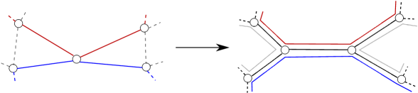
Figure 26. Projection from line graph coloring to cycle cover of $G$ satisfying the conditions of Theorem 1.1. The arrow indicates the mapping through $\pi_{\mathrm{chrom}}$.

As in the proof of Lemma 2.14 if the set of colored edges $\mathcal{C}$ defined a closed walk, the inverse operation would imply that there is a vertex in $\mathcal{L}(G)$ such that all incident edges have the same color. This is impossible by construction of $\Lambda^{\ast}$ such that all edges in $G$ are traversed by exactly two cycles from $\pi_{\mathrm{chrom}}(\Lambda)$. ∎

4. Outlook

There seems to be a connection to knot theory in all this. Effectively, with sufficient amounts of coffee and staring, the constructions proposed to disentangle the local issues in $\mathcal{L}^{(2)}_{red}$ resemble Seifert transformations used in Seifert’s algorithm for determining the genus of a knot. Also, by applying the transformations in an inverse sense, such that all joining reduced cliques become Type B self-intersections, and finally Type A self-intersections when they are all inverted, one obtains a single cycle in $\mathcal{L}^{(2)}_{red}$. From this single cycle, I propose to deduce a knot (but I am not sure how, yet).

The link between the genus of $G$ and the genus of said knot could be interesting. Indeed, for two graphs $G_{1}$, $G_{2}$ with $\mathcal{L}^{(2)}_{1,red}\stackrel{{\scriptstyle\sim}}{{=}}\mathcal{L}^{(2)}_{2,red}$ one would obtain the same knot, defining some sort of class of graphs based on their associated knot. This can be done for any simple connected graph with minimal degree greater or equal three by replacing every vertex with a cycle with length corresponding to the degree of the vertex and connecting each node of the cycle with one distinct neighbor of the original vertex. Therefore, this is not only for bridgeless cubic graphs but also in the case where the resulting graph is bridgeless. Conditions on the original graph for this to be the case, should be obtainable. This is one of the research paths, the author intends to follow aside from probabilistic view discussed hereinafter.

The motivation for the whole construction used in the proof of Proposition 2.17 comes from a connection between the notion of left hand paths and vertex orientations as discussed in [BM04] combined with a understanding of cubic graph with assigned vertex orientations as a spin system, since vertex orientations on cubic graphs are binary in their nature. One could, therefore, ask the question, whether a cycle double cover of $G$ can be seen as the equilibrium of some spin system relative to some Hamiltonian and the whole process of removing Type A self-intersections could be understood as an equivalent to Glauber dynamics.

As we have seen in Subsections 2.3.1 and 2.3.2, the necessary vectors of label inversions to reduce a Type A self-intersection are highly non-local in the sense that they not only impact some reduced clique and its neighbors but might be influencing reduced cliques very ”far away” from the Type A self-intersection, which we want to reduce. The correct view is on the level of cycles in $\mathcal{L}_{red}^{(2)}(G)$ and a configuration $\Gamma_{\Lambda}$ would be the set of cycles induced by labels $\Lambda$. This allows us to formulate the Hamiltonian as

$$\mathcal{H}(\Gamma_{\Lambda})=\sum_{\gamma_{i},\gamma_{j}\in\Gamma_{\Lambda}}\Phi(\gamma_{i},\gamma_{j})$$

where $\Phi$ is some symmetric interaction. This interaction $\Phi$ should be constructed from the cases discussed in Subsection 2.3.1. This results in a possibility of sampling cycle double covers, which are computationally still not approachable since the construction from Subsection 2.3.1 is not algorithmically feasible in the sense, that it needs non-polynomial effort in the size of the graph.

Appendix A Centered vertex-cuts and their lifts

The central technique for the proof of Proposition 2.17 were centered vertex cuts, build around a specific Type A self-intersections. Now we need to discuss and prove the topological result, which underlined the proof. A $v$ centered vertex cut $\mathbb{V}_{v}$ of $\mathcal{L}(G)$ with a bridge-free underlying graph $G$ satisfies necessarily $|\mathbb{V}_{v}|\in\{2,3,4\}$. We will consider in what follows all three cases where in each case there is one local structure which is added and the remaining cases are combinatorial combinations of previous cases. We call these combinatorial combinations the direct sum of any number of lower order cases and a direct sum can always be resolved as shown for the pair of balanced vertices shown hereinafter in the case $|\mathbb{V}_{v}|=2$.

Case 1 with $|\mathbb{V}_{v}|=2$:

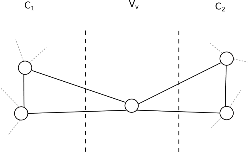
(a) A single vertex in the vertex cut with all its neighbors in one connected component or the other.

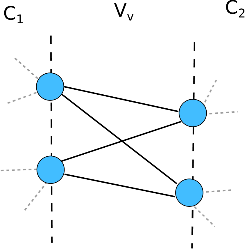
(b) Lift of a balanced vertex.

Figure 27. Cut vertex in $\mathbb{V}_{v}$ belonging to two triangles each in one connected component and its lift.

(a) The two vertices in $\mathbb{V}_{v}$ being neighbors.

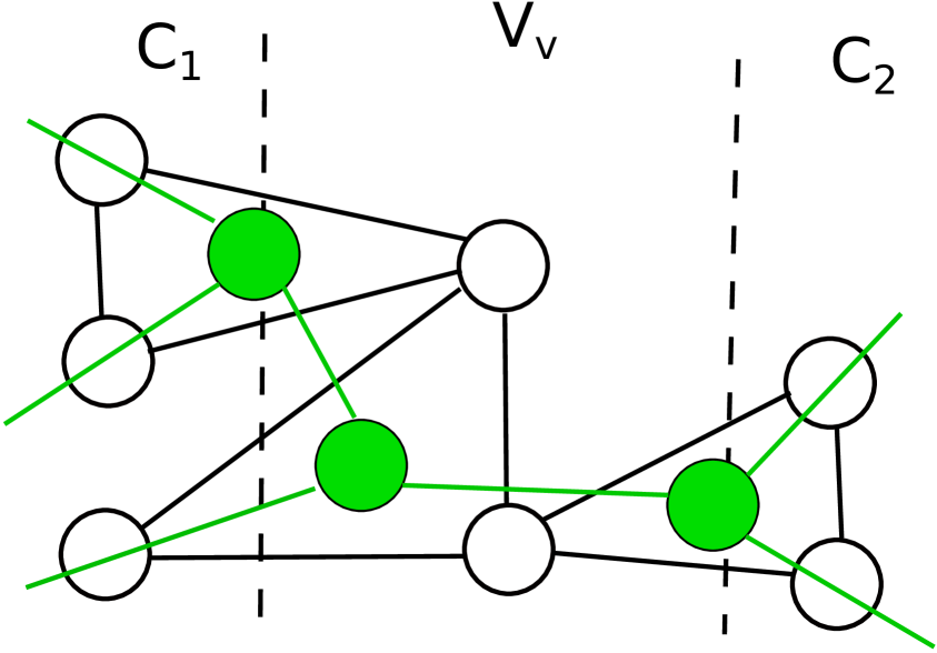
(b) It turns out that this configuration in the line graph $\mathcal{L}(G)$ implies a bridge in $G$ for $|\mathbb{V}_{v}|=2$. It will be relevant in the case $|\mathbb{V}_{v}|=3$.

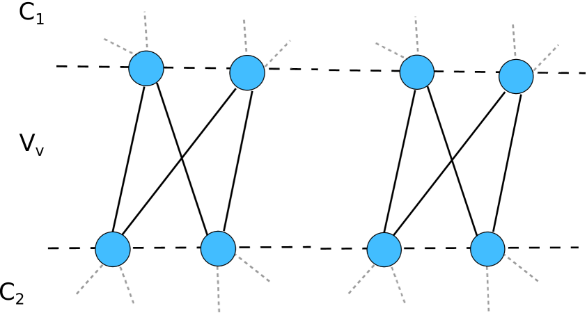
(c) Direct sum of lift of two balanced vertices. This situation is the simplest to resolve via label inversions and joining of cycles.

Figure 28. All possible situations for a cut vertex in $\mathbb{V}_{v}$ in $\mathcal{L}(G)$. A full triangle cannot lie within $\mathbb{V}_{v}$.

From Figure 28 we can see, that certain configurations for the centered vertex cut $\mathbb{V}_{v}$ are outside of conditions of the theorem, which we try to prove. In particular, whenever only the neighbors of one single vertex in $\mathbb{V}_{v}$ lie in $C_{1}$ or $C_{2}$, this vertex becomes a cut-vertex for $\mathcal{L}(G)$, as can be seen in Figure 28(b). Since $G$ is assumed to be bridgeless, this cannot happen. But, nonetheless, the configuration may occur as a building block for higher order cases of $|\mathbb{V}_{v}|=3$. They can then be resolved as the direct sum of two balanced vertices as shown in Figure 28(c).

Case 2 with $|\mathbb{V}_{v}|=3$:

(a) A balanced vertex in $\mathbb{V}_{v}$ with all its neighbors in the connected components.

(b) A semi-balanced vertex in $\mathbb{V}_{v}$ with one neighbor also in $\mathbb{V}_{v}$.

Figure 29. All possible situations for a cut vertex in $\mathbb{V}_{v}$ in $\mathcal{L}(G)$. A full triangle cannot lie within $\mathbb{V}_{v}$.

From Figure 29 we obtain further building blocks for the proof of Proposition 2.17.

Case 3 with $|\mathbb{V}_{v}|=4$: In the case that all three preceding cases do not apply to the $v$ centered vertex cut $\mathbb{V}_{v}$, we simply chose a neighbor $w_{v}$ of $v$ and $\mathbb{V}_{v}=\mathcal{N}_{w_{v}}$. This leads to a an ”empty” lift of the connected components $\{w_{v}\}$. Nonetheless, this suffices to make the conclusions about resolutions of Type A self-intersections.

(a) A balanced vertex in $\mathbb{V}_{v}$ with all its neighbors in the connected components.

(b) A semi-balanced vertex in $\mathbb{V}_{v}$ with one neighbor also in $\mathbb{V}_{v}$.

Figure 30. All possible situations for a cut vertex in $\mathbb{V}_{v}$ in $\mathcal{L}(G)$. A full triangle cannot lie within $\mathbb{V}_{v}$.

Note that at most two neighbors of each $v^{\prime}\in\mathbb{V}_{v}$ can belong to any connected component and the remaining ones have to be part of the vertex cut $\mathbb{V}_{v}$. Otherwise, due to the triangular structure of $\mathcal{L}(G)$, an edge would connect some $C_{i}$ and $C_{j}$, which is a contradiction to $\mathbb{V}_{v}$ being a vertex cut. Furthermore, that no triangle in $\mathcal{L}(G)$ belongs completely to $\mathbb{V}_{v}$ due to the minimality condition by the same logic as before. If we considered a vertex cut, which contains a triangle, then we can move one of the corners of the triangle to one of its adjacent connected components, i.e., in which it has a neighbor. Remember that this corner cannot have neighbors in two different connected components. This reduces the size of the vertex cut by $1$ while still being a vertex cut. This is a contradiction to minimality.

Finally, since $G$ is bridgeless, between any two $C_{i},C_{j}$ with $i\neq j$ there are at least two vertices $v^{\prime},w^{\prime}\in\mathbb{V}_{v}$ adjacent to vertices in $C_{i}$ and $C_{j}$. We only consider the connected components adjacent to $v$ of which there are exactly two and they are uniquely defined by our choice of $v$. We may, hence, assume without loss of generality, that there are exactly two connected components after deletion of any $v$-centered vertex cut $\mathbb{V}_{v}$. All types of cut vertices can be lifted to $\tilde{\mathcal{L}}_{red}^{(2)}(G)$ and take then the form of reduced cliques.

Statements and Declarations

This work was done independently after having finished my PhD in June 2022.
The author has no relevant financial or non-financial interests to disclose. The article was exclusively written by the mentioned author.

References

- [Har72] Robert Harary “Graph Theory” Addison Wesley, Massachusetts, 1972
- [Sze73] George Szekeres “Polyhedral decompositions of cubic graphs” In Bulletin of the Australian Mathematical Society 8.3 Cambridge University Press, 1973, pp. 367–387
- [Sey80] Paul D Seymour “Disjoint paths in graphs” In Discrete mathematics 29.3 Elsevier, 1980, pp. 293–309
- [BM04] Robert Brooks and Eran Makover “Random construction of Riemann surfaces” In Journal of Differential Geometry 68.1 Lehigh University, 2004, pp. 121–157