DeepIPCv2: LiDAR-powered Robust Environmental Perception and Navigational Control for Autonomous Vehicle

Abstract

We present DeepIPCv2, an autonomous driving model that perceives the environment using a LiDAR sensor for more robust drivability, especially when driving under poor illumination conditions where everything is not clearly visible. DeepIPCv2 takes a set of LiDAR point clouds as the main perception input. Since point clouds are not affected by illumination changes, they can provide a clear observation of the surroundings no matter what the condition is. This results in a better scene understanding and stable features provided by the perception module to support the controller module in estimating navigational control properly. To evaluate its performance, we conduct several tests by deploying the model to predict a set of driving records and perform real automated driving under three different conditions. We also conduct ablation and comparative studies with some recent models to justify its performance. Based on the experimental results, DeepIPCv2 shows a robust performance by achieving the best drivability in all driving scenarios. Furthermore, we will upload the codes to https://github.com/oskarnatan/DeepIPCv2.

I Introduction

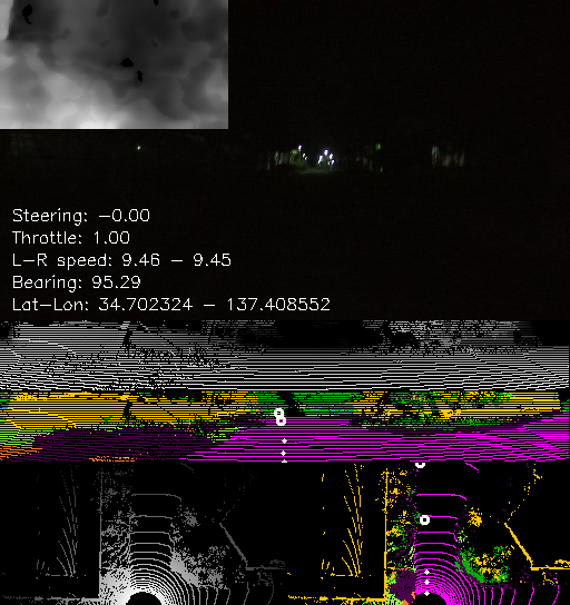
Figure 1: DeepIPCv2 perceives the environment by encoding a set of segmented point clouds that are projected into front and top-view perspectives. Then, the extracted features are used to estimate waypoints (white dots) and navigational controls to drive the vehicle following the route points (white hollow circles). Meanwhile, the RGBD image is only for record purposes. It shows how the RGBD camera fails in capturing surrounding information as it cannot provide a clearly visible set of RGB image and depth map. Instead, DeepIPCv2 employs a LiDAR sensor to provide point clouds that are not affected by poor illumination conditions. The detailed architecture of DeepIPCv2 can be seen in Fig. 2.

In autonomous driving, perception has always been a crucial stage as it is important to understand the surrounding before making any decisions [1][2][3][4]. A model can perceive the environment by performing many kinds of vision tasks such as object detection, semantic segmentation, and depth estimation [5][6][7][8]. To achieve a better performance, a lot of works have been proposed to improve scene understanding capability such as feeding a sequence of RGB images [9], training with multi-task learning paradigm [10], and using sensor fusion techniques [11] such as combining RGB images with dynamic vision sensor (DVS) images [12] or with depth (RGBD) images [13]. However, since these approaches rely on cameras, their performance may decrease or even fail under poor illumination conditions where everything is not clearly visible. One example of a camera-powered model for autonomous driving is our previous work namely DeepIPC (Deeply Integrated Perception and Control) [14]. Concisely, DeepIPC perceives the environment based on the captured RGBD images and drives the vehicle following a set of route points. However, its drivability decrease under low-light conditions as the camera is heavily affected by the illumination changes. Thus, an alternative sensor that is robust against illumination changes such as LiDAR is needed to perform a stable observation [15][16][17].

In this research, we propose an improved version of DeepIPC namely DeepIPCv2 where the improvisation is mainly intended to tackle the challenge of driving in poor illumination conditions. To be more specific, we modify the perception module by replacing RGBD encoders with LiDAR encoders. As shown in Fig. 1, the RGBD camera fails to provide a clearly visible set of RGB image and depth map. Hence, DeepIPCv2 uses a LiDAR sensor and employs a point cloud segmentation model to perceive the environment. This enables better reasoning as the model can distinguish traversable and non-traversable areas easily and avoid collision by knowing the existence of other objects around the ego vehicle. By encoding these point clouds, the perception module can provide stable and better features to the controller module for estimating waypoints and navigational control. Thus, DeepIPCv2 can maintain its drivability performance even when driving at night. We also modify the controller module by adding a set of command-specific multi-layer perceptrons (MLP) to improve the maneuverability of the model. The novelties of this work can be summarized as follows:

• We present DeepIPCv2, an improved version of DeepIPC [14] that takes LiDAR point clouds as the main perception input. Hence, it has better robustness against various illumination conditions as LiDAR is not affected by light illumination changes. This leads to better drivability as the controller module is provided with stable features in estimating navigational control properly.

• We demonstrate the utilization of LiDAR point clouds to achieve a robust environmental perception in perceiving the surroundings for autonomous driving. We conduct some ablation studies in point cloud projection and representation to obtain the best DeepIPC variant.

• We conduct a comparative study with other models to justify the drivability performance. All models must predict driving records and perform automated driving under three different conditions. The experimental results show that DeepIPCv2 achieves the best performance compared to other models in many criteria.

II Related Work

In this section, we review some works that lie in the field of point cloud processing. Then, we also provide reviews on some notable works that specifically use a LiDAR sensor for autonomous driving.

II-A LiDAR-powered Perception

LiDAR is a sensor that is considered to be more robust than an RGBD camera when dealing with poor illumination conditions. Unlike RGBD images, the point clouds are not affected by the illumination changes since the LiDAR has its own lasers as the light source to observe the environment [18][19]. Furthermore, together with plenty of point cloud segmentation models and projection techniques, many kinds of data representations can be formed to provide meaningful information [20][21]. In this research, we employ a point cloud segmentation model to achieve a robust environmental perception and scene understanding.

To date, there are plenty of works in the development of point cloud segmentation models. In the Semantic KITTI dataset [22], the current state-of-the-art is achieved by a model named 2DPASS [23]. However, its performance needs to be justified further in a very poor illumination condition as this model uses RGB images to assist the segmentation process. A point cloud segmentation model that only uses a LiDAR is proposed by Hou et. al. [24] which is currently the runner-up in the semantic point cloud segmentation challenge. Although it has a great performance, its size and latency are not suitable for performing real-time inference on a device with limited computation power. For deployment purposes, we need to consider the trade-off between speed and performance. Therefore, a model with great performance but causing a huge computation load is not preferable. Since we also seek robustness, the model must only use LiDAR in performing point cloud segmentation. Thus, we select PolarNet [25], a lightweight point cloud segmentation model that has an acceptable performance.

II-B End-to-end Model

With the rapid deep learning research, perception and control parts can be coupled together in an end-to-end manner to avoid manual integration that can lead to information loss. An end-to-end model is proven to have a better generalization as it can leverage the feature-sharing mechanism within its layers [26][27]. Moreover, each neuron can receive extra supervision from a multi-task loss formula that considers multiple performance criteria [28][29]. This results in a compact model that is relatively small but has a great performance which is preferable for real deployment.

Recent progress is made by Chitta et. al. [30] where a camera-powered end-to-end model is deployed to perform automated driving in a simulated environment. The RGB encoder of this model is guided by bird’s eye-view (BEV) semantic prediction to provide better features to the controller decoder. Although its performance in poor illumination conditions is promising, this model is practically hard to train as it is difficult to create BEV semantic ground truth in a real dataset. Then, a different work is proposed by Prakash et. al. where a camera-LiDAR fusion model named TransFuser [31][32] is deployed to handle various scenarios in autonomous driving. The camera is used to capture an RGB image in front of the vehicle, while the LiDAR is used to capture point clouds around the vehicle. The point clouds are projected into a 2-bin histogram over a 2D BEV grid with a fixed resolution [33]. With this configuration, the model can perceive from both front and BEV perspectives. Then, a certain transformer-based module is used to learn the relation between the RGB image and the projected point clouds to achieve a better perception. Considering its performance and robustness, we use TransFuser and its variants for comparative study purposes.

III Methodology

In this section, we describe the architecture of DeepIPCv2 and some metrics used to train and evaluate the model. Then, we also explain how the data is collected to train, validate, and test the model.

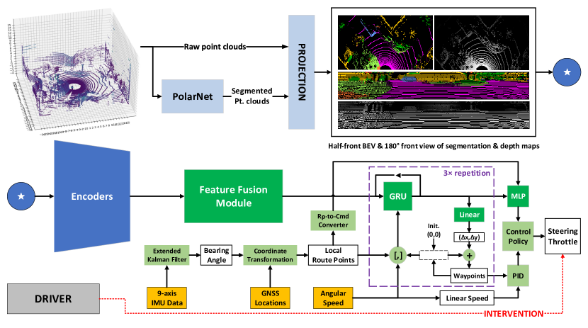
Figure 2: The architecture of DeepIPCv2. The blue and green blocks are the perception and controller modules respectively. Darker blocks are trainable, while light-colored blocks are not. In the perception module, PolarNet [25] is employed to support point cloud segmentation. Then, the architecture of encoders and feature fusion modules can be seen in Fig. 3.

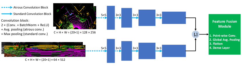
Figure 3: The architecture of the encoders and the feature fusion module. We use atrous convolution blocks [34] with different kernel sizes and dilation rates to capture low-level features from the projected point clouds that have vacant regions. Then, both top and front features are fused together and their relationship are learned by the feature fusion module.

III-A Proposed Model

III-A1 Perception Phase

Similar to DeepIPC [14], DeepIPCv2 is also a model that handles perception and control tasks simultaneously. However, unlike DeepIPC which takes an RGBD image, DeepIPCv2 takes a set of LiDAR point clouds to perceive the environment. Since LiDAR is not affected by poor illumination conditions, the perception module becomes more robust and can provide stable features to the controller module. Thus, the model can estimate waypoints and navigation control properly even when driving at night. As shown in Fig. 2, DeepIPCv2 employs PolarNet [25], a light-weight point cloud segmentation model pre-trained on the Semantic KITTI dataset [22] to segment LiDAR point clouds into twenty object classes as mentioned in Table I. Based on our previous work [35], perceiving the environment from more perspectives can improve perception and lead to better drivability. Hence, we project segmented point clouds to form one hot-encoded image-like array that shows front-view and bird’s eye-view (BEV) perspectives of the surrounding area. Each array is expressed as $\mathbb{R}\in\{0,1\}^{C\times H\times W}$, where $H\times W$ is the spatial dimension with $H\times W=64\times 512$ for the front-view array and $H\times W=128\times 256$ for the BEV array. Meanwhile, $C=21$ represents the number of channels that are responsible for twenty object classes and a logarithmic depth of the point clouds. In forming the BEV array, we consider an area of 16 meters to the front, left, and right of the vehicle. Meanwhile, for the front-view array, we consider all point clouds in front of the vehicle forming a 180-degree field of view.

To process these arrays, we use two different encoders that are made of atrous and standard convolution blocks as shown in Fig. 3. Atrous convolution blocks [34] are used to deal with some vacant regions in the projected LiDAR point clouds at the early encoding process. As the kernel sizes and dilation rates can be adjusted, an atrous convolution layer is more suitable than a standard convolution layer for extracting the features. Then, we also configure the pooling size after each convolution block to match the output size of both encoders. With this configuration, DeepIPCv2 has a better scene understanding capability as it can perceive from two different perspectives that clearly show traversable and non-traversable regions. Later, we conduct an ablation study by creating two additional model variants. The first variant only takes the logarithmic depth point clouds, while the other one only takes the segmented point clouds. After obtaining the best variant, we also conduct an extensive ablation study by comparing it with another variant that perceives the surroundings with one perspective, front or BEV. This is necessary to justify the importance of multi-view perception for better reasoning.

III-A2 Control Phase

The control phase begins by fusing both high-level perceptions features to produce a latent space composed of 192 feature elements that encapsulate the information of the surrounding based on two perspectives of view. This process is done by the feature fusion module that consists of a point-wise convolution layer, a global average pooling layer, and a dense layer. Then, we use the first and second route points, the left and right wheel’s angular speed, and predicted waypoints to bias the latent space in the gated recurrent unit (GRU) layer [36]. Finally, the biased latent space is decoded further by a set of command-specific multi-layer perceptrons (MLP) to estimate navigational control directly and by two linear layers to predict waypoints that will be translated into navigational control by a set of two PID controllers. To be noted, both MLP and PID controllers assume the model of the robotic vehicle as a nonholonomic unicycle since it has motorized rear wheels and omnidirectional front wheels. Thus, it cannot perform translational movement on the lateral axis, but it can move only along its longitudinal axis (forward and backward) and can rotate around a vertical axis passing through its center. As shown in Fig. 2, the process inside the purple box is looped three times as DeepIPCv2 predicts three waypoints. Two linear layers are used to predict $\Delta x$ and $\Delta y$ between the current waypoint and the next waypoint in the local coordinate. Thus, the exact coordinate of the next waypoint can be calculated with (1).

$$x_{i+1},y_{i+1}=(x_{i}+\Delta x),(y_{i}+\Delta y)$$ (1)

$\Theta=\frac{Wp_{1}+Wp_{2}}{2}$; $\theta=\tan^{-1}\big{(}\frac{\Theta[1]}{\Theta[0]}\big{)}$

$\gamma=1.75\times||Wp_{1}-Wp_{2}||_{F}$; $\nu=\frac{(\omega_{l}+\omega_{r})}{2}\times r$

if $Rp^{x}_{1}\leq-4m$ or $Rp^{x}_{2}\leq-8m$ then

       $Cmd=2$ (turn right)

else if $Rp^{x}_{1}\geq 4m$ or $Rp^{x}_{2}\geq 8m$ then

       $Cmd=1$ (turn left)

else

       $Cmd=0$ (go straight)

$\mathbf{MLP}_{\{ST,TH\}}=\mathbf{MLP}^{Cmd}(\mathcal{Z})$

$\mathbf{PID}_{\{ST,TH\}}=\mathbf{PID}^{Lat}(\theta-90),\mathbf{PID}^{Lon}(\gamma-\nu)$

if $\mathbf{MLP}_{TH}\geq 0.1$ and $\mathbf{PID}_{TH}\geq 0.1$ then

       if $|\mathbf{MLP}_{ST}|\geq 0.1$ and $|\mathbf{PID}_{ST}|<0.1$ then

             steering $=\mathbf{MLP}_{ST}$

            

       if $|\mathbf{MLP}_{ST}|<0.1$ and $|\mathbf{PID}_{ST}|\geq 0.1$ then

             steering $=\mathbf{PID}_{ST}$

            

       else

             steering $=\beta_{00}\mathbf{MLP}_{ST}+\beta_{10}\mathbf{PID}_{ST}$

            

       throttle $=\beta_{01}\mathbf{MLP}_{TH}+\beta_{11}\mathbf{PID}_{TH}$

      

else if $\mathbf{MLP}_{TH}\geq 0.1$ and $\mathbf{PID}_{TH}<0.1$ then

       steering $=\mathbf{MLP}_{ST}$; throttle $=\mathbf{MLP}_{TH}$

      

else if $\mathbf{MLP}_{TH}<0.1$ and $\mathbf{PID}_{TH}\geq 0.1$ then

       steering $=\mathbf{PID}_{ST}$; throttle $=\mathbf{PID}_{TH}$

      

else

       steering $=0$; throttle $=0$

      

• $Rp^{x}_{\{1,2\}}$: route point’s $x$ position in the local coordinate

• $Wp_{\{1,2\}}$: first and second waypoints

• $\mathcal{Z}$: GRU’s latent space

• $\omega_{\{l,r\}}$: left/right angular speed (rad/s)

• $r$: vehicle’s rear wheel radius (0.15 m)

• $\Theta$: aim point, a middle point between $Wp_{1}$ and $Wp_{2}$

• $\theta$: heading angle derived from the aim point $\Theta$

• $\gamma$: desired speed, 1.75 $\times$ Frobenius norm of $Wp_{1}$ and $Wp_{2}$

• $\nu$: linear speed (m/s), the mean of $\omega_{l}$ and $\omega_{r}$ multiplied by $r$

• $\beta\in\{0,...,1\}^{2\times 2}$ is a set of control weights initialized with:

• $\beta_{00}=\frac{\alpha_{1}}{\alpha_{1}+\alpha_{0}}$; $\beta_{10}=1-\beta_{00}$; $\beta_{01}=\frac{\alpha_{2}}{\alpha_{2}+\alpha_{0}}$; $\beta_{11}=1-\beta_{01}$

• where $\alpha_{0},\alpha_{1},\alpha_{2}$ are loss weights computed by MGN

• algorithm [37] (see Subsection III-C for more details)

Algorithm 1 Control Policy

To predict the first waypoint, the current waypoint is initialized with the vehicle position in the local coordinate which is always at (0,0). Then, the waypoints are processed by two PID controllers to produce a set of navigational control consisting of steering and throttle levels. Besides using PID controllers, DeepIPCv2 also predicts navigational control directly by decoding biased latent using MLP. However, unlike DeepIPC which employs only one MLP, DeepIPCv2 employs a set of command-specific MLPs for better maneuverability as demonstrated by Huang et. al [38]. Each of the command-specific MLPs act as a task-specific decoder that receives the same features from the same encoder. Then, since each decoder treats each action (turn left, turn right, or go straight) independently, the model has better maneuverability as it has more focus by deploying a dedicated MLP for each action. Moreover, this configuration can also deal with the imbalance number of actions in the driving records (e.g. the number of observation sets for go straight is larger than turn left or turn right). Meanwhile, the commands are generated automatically based on the route point’s $x$ position. The rule that generates the command and the policy which outputs the final action is summarized on Algorithm 1.

Furthermore, other measurement quantities and formulas are needed to transform the route points from the global GNSS coordinate to the local coordinate where the vehicle is always positioned at (0,0). To obtain the local coordinate for each route point $i$, the relative distance $\Delta x_{i}$ and $\Delta y_{i}$ between vehicle location $Ro$ and route point location $Rp_{i}$ need to be calculated first. Using the information of global longitude-latitude given by the GNSS receiver, the relative distance can be calculated with (2) and (3).

$$\Delta x_{i}=(Rp^{Lon}_{i}-Ro^{Lon})\times\frac{\mathcal{C}_{e}\times\cos(Ro^{Lat})}{360},$$ (2)

$$\Delta y_{i}=(Rp^{Lat}_{i}-Ro^{Lat})\times\frac{\mathcal{C}_{m}}{360},$$ (3)

where $\mathcal{C}_{e}$ and $\mathcal{C}_{m}$ are earth’s equatorial and meridional circumferences which are 40,075 and 40,008 km, respectively. Then, the local coordinate of each route point $Rp^{(x,y)}_{i}$ can be obtained by applying a rotation matrix as in (4).

$$\begin{bmatrix}Rp^{x}_{i}\\ Rp^{y}_{i}\end{bmatrix}=\begin{bmatrix}\cos(\theta_{ro})&-\sin(\theta_{ro})\\ \sin(\theta_{ro})&\cos(\theta_{ro})\end{bmatrix}^{T}\begin{bmatrix}\Delta x_{i}\\ \Delta y_{i}\end{bmatrix},$$ (4)

where $\theta_{ro}$ is the vehicle’s absolute orientation to the north pole (bearing angle). In this research, the bearing angle is estimated by the extended Kalman filter (EKF) based on the measurement of 3-axial acceleration, angular speed, and magnetic field retrieved from a 9-axis IMU sensor. To be noted, due to the GNSS inaccuracy and noisy IMU measurements the global-to-local transformation may not be perfect. Thus, the model is expected to learn implicitly how to compensate for this issue during the training process.

III-B Dataset

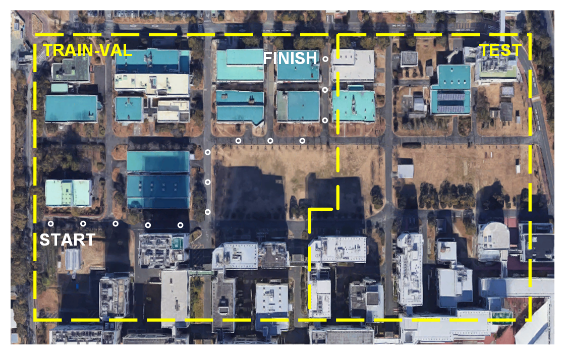
Figure 4: The experiment areas (more detail at https://goo.gl/maps/9rXobdhP3VYdjXn48). White hollow circles represent a route that consists of a start, finish, and route points.

A dataset that consists of expert driving records is needed for behavior cloning [39][40][41][42]. To create the dataset for training, validation, and test (train-val-test), we record observation data while driving the robotic vehicle at a speed of 1.25 m/s in an area inside Toyohashi University of Technology, Japan as shown in Fig. 4. We record the driving data at noon, in the evening, and at night to vary the experiment conditions. In the train-val area, there are 12 different routes where the driving data is recorded one time for each condition. Meanwhile, in the test area, there are 6 different routes where the driving data is recorded three times for each condition. Each route has a set of route points with 12 meters gap that shows the path to the finish point. The vehicle must follow this path to complete the route.

Recorded at a rate of 4 Hz, one sample of observation data is composed of a set of LiDAR point clouds, GNSS latitude-longitude, 9-axis IMU measurement, left and right wheel’s angular speeds, and the level of steering and throttle. We also record the RGB image which is used by another model for comparison. Then, as the ground truth for the waypoints prediction task, we use the vehicle’s trajectory location in one second, two seconds, and three seconds in the future (relative to the vehicle’s current location at the current time). The trajectory is estimated by a built-in IMU-based odometry algorithm embedded in the robotic vehicle. Meanwhile, as the ground truth for the navigational control estimation task, we use the record of steering and control levels at the time. The devices used to retrieve observation data are mentioned in Table I. Meanwhile, how they are mounted on the vehicle can be seen in Fig. 5.

TABLE I: Dataset Information

Conditions	Noon, evening, night
Total routes	12 (train-val) and 6 (test)
$\mathcal{N}$ Samples*	19781 (train), 9695 (val), 29123 (test)
Devices	WHILL model C2 (+ rotary encoder)
	Velodyne LiDAR HDL-32e
	Stereolabs Zed RGBD camera
	U-blox Zed-F9P GNSS receiver
	Witmotion HWT905 9-axis IMU sensor
Object classes	None, car, bicycle, motorcycle, truck, other vehicle, person, bicyclist, motorcyclist, road, parking, sidewalk, ground, building, fence, vegetation, trunk, terrain, pole, traffic sign

• *$\mathcal{N}$ Samples is the number of observation sets. One observation set consists of RGBD image, GNSS location, 9-axis IMU measurement, wheel’s angular speed, and the level of steering and throttle.

III-C Training

A multi-task loss function used to supervise DeepIPCv2 during the training process is formulated with (5).

$$\mathcal{L}_{MTL}=\alpha_{0}\mathcal{L}_{WP}+\alpha_{1}\mathcal{L}_{ST}+\alpha_{2}\mathcal{L}_{TH},$$ (5)

TABLE II: Model Specification

Model	Variant	Parameters$\downarrow$	Input/Sensor	Output
TransFuser [31][32]	Late Fusion	32.64M	LiDAR, RGB, GNSS, IMU, Rotary	Waypoints, Steering, Throttle
	Transformer	66.23M	LiDAR, RGB, GNSS, IMU, Rotary	Waypoints, Steering, Throttle
DeepIPCv2	Log. Depth	5.91M	LiDAR, GNSS, IMU, Rotary	Waypoints, Steering, Throttle
	Segmentation	5.95M $+$14M*	LiDAR, GNSS, IMU, Rotary	Segmentation*, Waypoints, Steering, Throttle
	Segmentation $+$ Log. Depth	5.96M $+$14M*	LiDAR, GNSS, IMU, Rotary	Segmentation*, Waypoints, Steering, Throttle

• *These model variants employ PolarNet [25] which has total parameters of around 14 million to perform point cloud segmentation.

• We replicate TransFuser [31][32] based on the codes shared by the authors at https://github.com/autonomousvision/transfuser.

• We cannot compute the inference speed fairly due to fluctuating GPU computation, hence we assume that smaller models will consume less GPU memory footprint and infer faster. Furthermore, as we limit the maximum speed to only 1.25m/s (the same as the data collection process), a high FPS rate is not necessary for driving the robotic vehicle.

where $\alpha_{0,1,2}$ are loss weights tuned adaptively by an algorithm called modified gradient normalization (MGN) [37] to ensure that all tasks can be learned at the same pace. To supervise waypoints prediction, we use L1 loss as in (6).

$$\mathcal{L}_{WP}=\frac{1}{N}\sum_{i=1}^{N}|y_{i}-\hat{y}_{i}|,$$ (6)

where $N$ is equal to 6 as there are three waypoints that have x,y elements in the local coordinate. Meanwhile, $y_{i}$ and $\hat{y}_{i}$ are the ground truth and the prediction of component $i$ respectively. Similarly, we also use L1 loss to supervise navigational control estimation formulated with (7).

$$\mathcal{L}_{\{ST,TH\}}=|\hat{y}-y|$$ (7)

Keep in mind that there is no averaging process as there is only one element for each output (steering and throttle). The model is implemented with PyTorch framework [43] and trained on NVIDIA RTX 3090 with a batch size of 10. We use Adam optimizer [44] with decoupled weight decay of 0.001 [45]. The initial learning rate is set to 0.0001 and reduced by half if the validation $\mathcal{L}_{MTL}$ is not dropping in 5 epochs in a row. The train-val process will be stopped if there is no drop on the validation $\mathcal{L}_{MTL}$ in 30 epochs in a row.

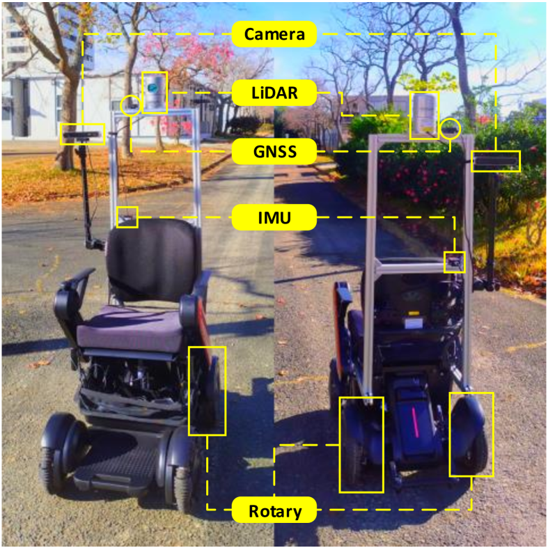
Figure 5: Sensor placement on the robotic vehicle. The vehicle is categorized as a nonholonomic unicycle since it has motorized rear wheels and omnidirectional front wheels.

III-D Evaluation and Scoring

The evaluation is conducted under three different conditions (noon, evening, night). We consider two different evaluations namely offline and online tests. In the offline test, DeepIPCv2 is deployed to predict expert driving records on the test routes. Each record has six different routes that are recorded on different days to vary the situation. Then, the performance is defined by the total metric (TM) score as in (8).

$$TM=MAE_{WP}+MAE_{ST}+MAE_{TH}$$ (8)

where $MAE$ stands for mean absolute error (also known as L1 loss) which can be computed with (6) for $MAE_{WP}$ and (7) for $MAE_{ST}$ and $MAE_{TH}$. The smaller the total metric score means the better the performance. Meanwhile, in the online test, DeepIPCv2 must drive the vehicle and complete six different routes. We determine the drivability performance by counting the number of interventions and intervention time needed to prevent any collisions. The smaller the number of interventions and intervention time means the better the performance. Then, the final score for offline and online tests must be averaged as the evaluation is conducted three times.

TABLE III: Multi-task Performance Score 1

Condition	Model	Variant	Total Metric$\downarrow$	$MAE_{WP}\downarrow$	$MAE_{ST}\downarrow$	$MAE_{TH}\downarrow$
Noon	TransFuser [31][32]	Late Fusion	0.211 $\pm$0.007	0.087	0.097	0.027
		Transformer	0.192 $\pm$0.006	0.073	0.093	0.026
	DeepIPCv2	Logarithmic Depth	0.276 $\pm$0.004	0.116	0.123	0.037
		Segmentation	0.168 $\pm$0.005	0.059	0.085	0.024
		Segmentation $+$ Logarithmic Depth	0.196 $\pm$0.007	0.074	0.095	0.026
Evening	TransFuser [31][32]	Late Fusion	0.213 $\pm$0.006	0.089	0.097	0.027
		Transformer	0.193 $\pm$0.008	0.073	0.094	0.026
	DeepIPCv2	Logarithmic Depth	0.281 $\pm$0.007	0.119	0.126	0.036
		Segmentation	0.167 $\pm$0.006	0.059	0.084	0.023
		Segmentation $+$ Logarithmic Depth	0.199 $\pm$0.008	0.076	0.097	0.026
Night	TransFuser [31][32]	Late Fusion	0.218 $\pm$0.002	0.090	0.099	0.029
		Transformer	0.197 $\pm$0.003	0.075	0.094	0.028
	DeepIPCv2	Logarithmic Depth	0.278 $\pm$0.005	0.115	0.125	0.038
		Segmentation	0.170 $\pm$0.002	0.059	0.086	0.026
		Segmentation $+$ Logarithmic Depth	0.198 $\pm$0.004	0.072	0.097	0.028

As mentioned in Subsection III-A, we create two model variants for the ablation study. The first variant only takes the logarithmic depth point clouds while the second variant only takes the segmented point clouds. Then, after obtaining the best variant, we conduct another ablation study by comparing it with other variants that perceive the surroundings using only one perspective, front or BEV. Furthermore, we also conduct a comparative study by replicating TransFuser [31][32] to compare with. Briefly, TransFuser is a camera-LiDAR fusion model that takes an RGB image and a set of point clouds. It perceives the environment from two different perspectives where the front view information is given by the RGB camera and the BEV information is given by the LiDAR. TransFuser fuses RGB images and LiDAR point clouds features using several transformer modules. We also replicate its variant called late fusion, where the features are fused with a simple element-wise summation. The specification of DeepIPCv2 and TransFuser variants can be seen in Table II.

IV Result and Discussion

IV-A Offline Test

An offline test is used to measure how good the model is in mimicking an expert by predicting several driving records made for testing purposes. We measure the model performance by calculating the MAE on waypoints prediction and navigational control estimation together with the total metric (TM) score as explained in Subsection III-D. Since there are three driving records for each condition, the final score for each condition is averaged from all inference results.

Based on Table III, the DeepIPCv2 variant that only takes segmented point clouds achieves the best performance by having the lowest TM score in all conditions. The other two DeepIPCv2 variants that take logarithmic depth point clouds fall behind and the depth-only variant performs the worst. This pattern shows that processing logarithmic depth reduces overall model performance due to conflicting features between the segmentation map and the depth map extracted by the encoders. This also means that the data representation given by the projected point clouds in the segmentation map is more than enough and better than the combination with logarithmic depth. However, this hypothesis needs to be justified further by applying different encoder architectures to process the projected point clouds. Meanwhile, amongst TransFuser variants, the variant that employs transformer modules to fuse image and point cloud features achieves a better performance than the variant that only uses a simple element-wise summation. Although it costs a lot of parameters to train, the transformer modules can improve the model’s reasoning as it understands the relationship between the front view and BEV perspectives.

TABLE IV: Multi-task Performance Score 2

Condition	Perspective	Total Metric$\downarrow$	$MAE_{WP}\downarrow$	$MAE_{ST}\downarrow$	$MAE_{TH}\downarrow$
Noon	Front	0.258 $\pm$0.006	0.062	0.173	0.023
	BEV	0.171 $\pm$0.006	0.063	0.084	0.024
	Front $+$ BEV	0.168 $\pm$0.005	0.059	0.085	0.024
Evening	Front	0.258 $\pm$0.014	0.063	0.173	0.022
	BEV	0.171 $\pm$0.005	0.062	0.085	0.023
	Front $+$ BEV	0.167 $\pm$0.006	0.059	0.084	0.023
Night	Front	0.263 $\pm$0.005	0.061	0.177	0.025
	BEV	0.174 $\pm$0.004	0.062	0.086	0.026
	Front $+$ BEV	0.170 $\pm$0.002	0.059	0.086	0.026

In the comparison across different conditions, the total metric scores for both TransFuser variants consistently become higher from predicting noon records to night records. Although the gap is not too far from one another, this pattern shows that TransFuser which relies on RGB images gets a performance drop when the illumination condition is poor. This result is as expected since the RGB camera is sensitive to illumination changes. Unlike TransFuser, DeepIPCv2 is more robust against poor illumination conditions as it only relies on LiDAR to perceive the environment. However, there is no clear pattern amongst DeepIPCv2 variants as their performance differs on every condition. DeepIPCv2 performance is more affected by road situations rather than illumination conditions. This is supported by the fact that two DeepIPCv2 variants have the best performance at night when there is not so much traffic on the road.

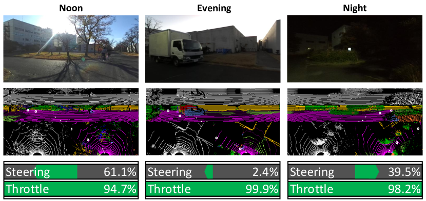
Figure 6: Driving footage. Noon: DeepIPCv2 makes a left turn following two route points located on the left side of the vehicle. Evening: A moment when we are going to intervene in DeepIPCv2 as it fails to make a hard left turn to compromise a narrowing path caused by a stopping truck. Night: DeepIPCv2 makes a right turn following two route points while maintaining the distance from the road boundaries. To be noted, the RGB images are only for record purposes. We share some of the driving records including the comparison with TransFuser [31][32] at https://youtu.be/IsZ1HP5QjWc.

IV-A1 More Perspectives, Better Reasoning

To understand the importance of perceiving from multiple perspectives of view, we also conduct an extensive ablation study by creating two more DeepIPCv2 variants that take one perspective of view. Hence, the model can only perceive the environment based on the front-view perspective or the top-view/bird’s eye view (BEV) perspective. We develop these variants based on DeepIPCv2 variant that takes the point cloud segmentation map. Table IV shows that the model variant that perceives the environment from both front and BEV perspectives has the lowest total metric score meaning that it achieves the best performance compared to the variants which only use one perspective. This result is in line with the findings in our previous work [14][35] and strengthens the importance of perceiving from multiple perspectives of view.

To be more detailed, DeepIPCv2 variant that perceives from the front-view perspective has the worst performance as its steering estimation is heavily affected by the absence of BEV perception features. Without these features, the controller module faces difficulties in estimating the steering angle which lies in the BEV coordinate. Meanwhile, DeepIPCv2 variant that perceives from the BEV perspective is slightly behind the best variant. Although it has a comparable performance in steering angle and throttle level estimation, this variant fails to estimate waypoints properly as predicting future vehicle position needs the combination of both front and BEV perception features that consider more aspects of driving. Therefore, judging from this result and analysis, we pick the DeepIPCv2 variant that only takes segmented point clouds and perceives the environment from multiple perspectives of view for further comparison in the online test. Meanwhile, we pick TransFuser variant that employs transformer modules as the comparator to study the importance of data modality and representation in performing real-world autonomous driving.

IV-B Online Test

An online test is made for evaluating the drivability performance of the model after imitating expert behavior in driving a vehicle during the training process. The best variant of DeepIPCv2 and TransFuser are evaluated by being deployed for automated driving in real environments. Each model must be able to handle various situations and conditions when driving a vehicle from the starting point to the finish point by following a set of route points. Similar to the offline test, we conduct the test three times on six different routes for each condition. However, the drivability performance is justified by the number of interventions and how long the interventions are. The best performance is determined by the lowest number of interventions and the shortest time of intervention. Keep in mind that the result of the online test may not be in line with the result of the offline test. This is because any decisions made on every observation state in the online test will affect the next observation state. Meanwhile, in the offline test, although the model makes a wrong prediction on a certain set of observations, it will not affect anything as the observation is already fixed in the driving records. Furthermore, some driving footage made by DeepIPCv2 can be seen in Fig. 6.

TABLE V: Drivability Score

Condition	Model	Intervention$\downarrow$
		Count	Time (secs)
Noon	TransFuser [31][32]	1.389 $\pm$0.208	3.537 $\pm$0.648
	DeepIPCv2	1.000 $\pm$0.236	2.389 $\pm$0.831
Evening	TransFuser [31][32]	1.222 $\pm$0.079	3.093 $\pm$0.457
	DeepIPCv2	0.944 $\pm$0.157	2.407 $\pm$0.466
Night	TransFuser [31][32]	1.889 $\pm$0.283	4.556 $\pm$0.181
	DeepIPCv2	0.667 $\pm$0.136	1.870 $\pm$0.340

Table V shows a clear pattern for each model when driving under different conditions. For DeepIPCv2 which is not affected by illumination conditions, the best drivability is achieved at night when there is not so much traffic on the road. Then, it has lower performance at noon and in the evening as it is affected by denser traffic on the road. Meanwhile, as for TransFuser which relies on the RGB camera, better performance is achieved when the model drives at noon and in the evening. Thanks to enough light illumination, the RGB camera can capture an image clearly so that TransFuser can maintain its drivability. However, TransFuser performance is degraded when driving at night as it fails to capture the information in front of the vehicle due to poor illumination conditions. Therefore, as the perception module cannot extract useful features, the controller module also fails to estimate navigational control properly.

In all conditions, DeepIPCv2 has the best performance based on the lowest intervention count and intervention time compared to TransFuser. This means that a set of segmented point clouds projected into two different perspectives of view contains more valuable information than a combination of a raw RGB image and a 2-bin point cloud histogram. By projecting the segmented point clouds to form image-like arrays that contain a unique class on each layer, the model has a better scene understanding capability as it can distinguish traversable and non-traversable areas clearly and lead to better driving performance. This also shows that data representation (e.g. segmented and projected point clouds) is matter and more meaningful than a combination of some data modalities (e.g. RGB images and LiDAR point clouds) but still in their raw form or improperly pre-processed.

V Conclusion

We propose DeepIPCv2 which perceives the environment using LiDAR for more robust drivability. DeepIPCv2 is evaluated by predicting driving records and performing automated driving. To justify its performance, we conduct ablation and comparative studies with other models under different conditions to vary the situations.

Based on the experimental results, we disclose that using LiDAR to perceive the environment increases the model’s robustness. Unlike an RGB camera, LiDAR is not affected by poor illumination conditions. Thus, the perception module can provide stable features to the controller module in estimating navigational control properly. Therefore, the model can maintain its drivability even when driving at night. Meanwhile, the performance of a camera-powered model drops as it fails to perceive the surrounding area. Then, we also disclose that perceiving the environment with segmented point clouds that are projected into multi-view perspectives is better than a combination of raw RGB images and 2-bin histogram point clouds. As the model has better reasoning, the overall driving performance is increased.

In the future, more crowded environments and more adversarial scenarios (e.g. pedestrians crossing the street suddenly) can be used to test the model further. As the driving challenges increased, the model also needs to be enhanced with a sensor that can detect event changes such as a DVS camera to improve the perception and result in better drivability. Furthermore, better encoders and fusion techniques might be necessary to handle more varied data with different modalities and representations.

Oskar Natan (Member, IEEE) received his B.A.Sc. degree in electronics engineering and M.Eng. degree in electrical engineering from the Electronic Engineering Polytechnic Institute of Surabaya, Indonesia in 2017 and 2019, respectively. In 2023, he received his Ph.D. degree in computer science and engineering from Toyohashi University of Technology, Japan. Since January 2020, he has been serving as a Lecturer at the Department of Computer Science and Electronics, Gadjah Mada University, Indonesia. His research interests lie in the fields of sensor fusion and end-to-end systems.

Jun Miura (Member, IEEE) received his B.Eng. degree in mechanical engineering and his M.Eng. and Dr.Eng. degrees in information engineering from The University of Tokyo, Japan, in 1984, 1986, and 1989, respectively. From 1989 to 2007, he was with the Department of Computer-controlled Mechanical Systems, Osaka University, Japan, first as a Research Associate and later as an Associate Professor. From March 1994 to February 1995, he was a Visiting Scientist with the Department of Computer Science, Carnegie Mellon University, USA. In 2007, he became a Professor with the Department of Computer Science and Engineering, Toyohashi University of Technology, Japan. He has authored or coauthored more than 260 scientific articles in the field of robotics and artificial intelligence in internationally reputable journals and conferences. He was the recipient of numerous awards, including the Best Paper Award from the Robotics Society of Japan in 1997, the Best Paper Award Finalist at ICRA 1995, and the Best Service Robotics Paper Award Finalist at ICRA 2013.

References

- [1] J. Horgan, C. Hughes, J. McDonald, and S. Yogamani, “Vision-based driver assistance systems: Survey, taxonomy and advances,” in Proc. IEEE Intell. Transp. Syst. Conf. (ITSC), Gran Canaria, Spain, Sep. 2015, pp. 2032–2039.
- [2] Y. Cui, R. Chen, W. Chu, L. Chen, D. Tian, Y. Li, and D. Cao, “Deep learning for image and point cloud fusion in autonomous driving: A review,” IEEE Trans. Intell. Transp. Syst., vol. 23, no. 2, pp. 722–739, Feb. 2022.
- [3] K. Muhammad, T. Hussain, H. Ullah, J. D. Ser, M. Rezaei, N. Kumar, M. Hijji, P. Bellavista, and V. H. C. de Albuquerque, “Vision-based semantic segmentation in scene understanding for autonomous driving: Recent achievements, challenges, and outlooks,” IEEE Trans. Intell. Transp. Syst., vol. 23, no. 12, pp. 22 694–22 715, Dec. 2022.
- [4] D. Omeiza, H. Webb, M. Jirotka, and L. Kunze, “Explanations in autonomous driving: A survey,” IEEE Trans. Intell. Transp. Syst., vol. 23, no. 8, pp. 10 142–10 162, Aug. 2022.
- [5] G. Adam, V. Chitalia, N. Simha, A. Ismail, S. Kulkarni, V. Narayan, and M. Schulze, “Robustness and deployability of deep object detectors in autonomous driving,” in Proc. IEEE Intell. Transp. Syst. Conf. (ITSC), Auckland, New Zealand, Oct. 2019, pp. 4128–4133.
- [6] C. Wang and N. Aouf, “Fusion attention network for autonomous cars semantic segmentation,” in Proc. IEEE Intell. Veh. Symp. (IV), Aachen, Germany, Jul. 2022, pp. 1525–1530.
- [7] O. Natan, D. U. K. Putri, and A. Dharmawan, “Deep learning-based weld spot segmentation using modified UNet with various convolutional blocks,” ICIC Express Letters Part B: Applications, vol. 12, no. 12, pp. 1169–1176, Dec. 2021.
- [8] A. Gurram, A. F. Tuna, F. Shen, O. Urfalioglu, and A. M. López, “Monocular depth estimation through virtual-world supervision and real-world SfM self-supervision,” IEEE Trans. Intell. Transp. Syst., vol. 23, no. 8, pp. 12 738–12 751, Aug. 2022.
- [9] H.-k. Chiu, E. Adeli, and J. C. Niebles, “Segmenting the future,” IEEE Robot. and Autom. Lett., vol. 5, no. 3, pp. 4202–4209, Jul. 2020.
- [10] T.-J. Song, J. Jeong, and J.-H. Kim, “End-to-end real-time obstacle detection network for safe self-driving via multi-task learning,” IEEE Trans. Intell. Transp. Syst., vol. 23, no. 9, pp. 16 318–16 329, Sep. 2022.
- [11] S. Xu, D. Zhou, J. Fang, J. Yin, Z. Bin, and L. Zhang, “FusionPainting: Multimodal fusion with adaptive attention for 3D object detection,” in Proc. IEEE Intell. Transp. Syst. Conf. (ITSC), Indianapolis, USA, Oct. 2021, pp. 3047–3054.
- [12] O. Natan and J. Miura, “Semantic segmentation and depth estimation with RGB and DVS sensor fusion for multi-view driving perception,” in Proc. Asian Conf. Pattern Recog. (ACPR), Jeju Island, South Korea, Nov. 2021, pp. 352–365.
- [13] L. Sun, K. Yang, X. Hu, W. Hu, and K. Wang, “Real-time fusion network for RGB-D semantic segmentation incorporating unexpected obstacle detection for road-driving images,” IEEE Robot. and Autom. Lett., vol. 5, no. 4, pp. 5558–5565, Oct. 2020.
- [14] O. Natan and J. Miura, “DeepIPC: Deeply integrated perception and control for an autonomous vehicle in real environments,” arXiv preprint, 2022. [Online]. Available: https://arxiv.org/abs/2207.09934
- [15] Z. He, X. Fan, Y. Peng, Z. Shen, J. Jiao, and M. Liu, “EmPointMovSeg: Sparse tensor-based moving-object segmentation in 3-D LiDAR point clouds for autonomous driving-embedded system,” IEEE Trans. Comput.-Aided Des. Integr. Circuits Syst., vol. 42, no. 1, pp. 41–53, Jan. 2023.
- [16] S. Zhou, H. Xu, G. Zhang, T. Ma, and Y. Yang, “Leveraging deep convolutional neural networks pre-trained on autonomous driving data for vehicle detection from roadside LiDAR data,” IEEE Trans. Intell. Transp. Syst., vol. 23, no. 11, pp. 22 367–22 377, Nov. 2022.
- [17] G. Xian, C. Ji, L. Zhou, G. Chen, J. Zhang, B. Li, X. Xue, and J. Pu, “Location-guided LiDAR-based panoptic segmentation for autonomous driving,” IEEE Trans. Intell. Veh., vol. 8, no. 2, pp. 1473–1483, Feb. 2023.
- [18] R. W. Wolcott and R. M. Eustice, “Robust LiDAR localization using multiresolution Gaussian mixture maps for autonomous driving,” Int. J. Rob. Res., vol. 36, no. 3, pp. 292–319, Apr. 2017.
- [19] S. McCrae and A. Zakhor, “3D object detection for autonomous driving using temporal LiDAR data,” in Proc. Inter. Conf. Image Processing (ICIP), Abu Dhabi, UAE, Oct. 2020, pp. 2661–2665.
- [20] Y. Li, L. Ma, Z. Zhong, F. Liu, M. A. Chapman, D. Cao, and J. Li, “Deep learning for LiDAR point clouds in autonomous driving: A review,” IEEE Trans. Neural Networks and Learning Syst., vol. 32, no. 8, pp. 3412–3432, Aug. 2021.
- [21] Y. Li and J. Ibanez-Guzman, “Lidar for autonomous driving: The principles, challenges, and trends for automotive lidar and perception systems,” IEEE Signal Process. Mag., vol. 37, no. 4, pp. 50–61, Jul. 2020.
- [22] J. Behley, M. Garbade, A. Milioto, J. Quenzel, S. Behnke, J. Gall, and C. Stachniss, “Towards 3D LiDAR-based semantic scene understanding of 3D point cloud sequences: The SemanticKITTI Dataset,” The International Journal on Robotics Research, vol. 40, no. 8-9, pp. 959–967, Apr. 2021.
- [23] X. Yan, J. Gao, C. Zheng, C. Zheng, R. Zhang, S. Cui, and Z. Li, “2DPASS: 2D priors assisted semantic segmentation on LiDAR point clouds,” in Proc. European Conf. Comput. Vision (ECCV), Tel Aviv, Israel, Oct. 2022, pp. 677–695.
- [24] Y. Hou, X. Zhu, Y. Ma, C. C. Loy, and Y. Li, “Point-to-voxel knowledge distillation for LiDAR semantic segmentation,” in Proc. IEEE/CVF Conf. Comput. Vision and Pattern Recog. (CVPR), New Orleans, USA, Jun. 2022, pp. 8469–8478.
- [25] Y. Zhang, Z. Zhou, P. David, X. Yue, Z. Xi, B. Gong, and H. Foroosh, “PolarNet: An improved grid representation for online LiDAR point clouds semantic segmentation,” in Proc. IEEE/CVF Conf. Comput. Vision and Pattern Recog. (CVPR), Seattle, USA, Jun. 2020, pp. 9598–9607.
- [26] A. Tampuu, T. Matiisen, M. Semikin, D. Fishman, and N. Muhammad, “A survey of end-to-end driving: Architectures and training methods,” IEEE Trans. Neural Networks and Learning Syst., vol. 33, no. 4, pp. 1364–1384, Apr. 2022.
- [27] S. Teng, L. Chen, Y. Ai, Y. Zhou, Z. Xuanyuan, and X. Hu, “Hierarchical interpretable imitation learning for end-to-end autonomous driving,” IEEE Trans. Intell. Veh., vol. 8, no. 1, pp. 673–683, Jan. 2023.
- [28] K. Ishihara, A. Kanervisto, J. Miura, and V. Hautamaki, “Multi-task learning with attention for end-to-end autonomous driving,” in Proc. IEEE/CVF Conf. Comput. Vision and Pattern Recog. Workshops (CVPRW), Nashville, USA, Jun. 2021, pp. 2896–2905.
- [29] E. Kargar and V. Kyrki, “Increasing the efficiency of policy learning for autonomous vehicles by multi-task representation learning,” IEEE Trans. Intell. Veh., vol. 7, no. 3, pp. 701–710, Sep. 2022.
- [30] K. Chitta, A. Prakash, and A. Geiger, “NEAT: Neural attention fields for end-to-end autonomous driving,” in Proc. IEEE/CVF Inter. Conf. Comput. Vision (ICCV), Montreal, Canada, Oct. 2021, pp. 15 773–15 783.
- [31] A. Prakash, K. Chitta, and A. Geiger, “Multi-modal fusion transformer for end-to-end autonomous driving,” in Proc. IEEE/CVF Conf. Comput. Vision and Pattern Recog. (CVPR), Nashville, USA, Jun. 2021, pp. 7073–7083.
- [32] K. Chitta, A. Prakash, B. Jaeger, Z. Yu, K. Renz, and A. Geiger, “TransFuser: Imitation with transformer-based sensor fusion for autonomous driving,” IEEE Trans. Pattern Anal. Mach. Intell., 2022. [Online]. Available: https://doi.org/10.1109/TPAMI.2022.3200245
- [33] N. Rhinehart, R. Mcallister, K. Kitani, and S. Levine, “PRECOG: Prediction conditioned on goals in visual multi-agent settings,” in Proc. IEEE/CVF Inter. Conf. Comput. Vision (ICCV), Seoul, South Korea, Nov. 2019, pp. 2821–2830.
- [34] L.-C. Chen, G. Papandreou, I. Kokkinos, K. Murphy, and A. L. Yuille, “DeepLab: Semantic image segmentation with deep convolutional nets, atrous convolution, and fully connected CRFs,” IEEE Trans. Pattern Anal. Mach. Intell., vol. 40, no. 4, pp. 834–848, Apr. 2018.
- [35] O. Natan and J. Miura, “End-to-end autonomous driving with semantic depth cloud mapping and multi-agent,” IEEE Trans. Intell. Veh., vol. 8, no. 1, pp. 557–571, Jan. 2022.
- [36] K. Cho, B. van Merrienboer, D. Bahdanau, and Y. Bengio, “On the properties of neural machine translation: Encoder-decoder approaches,” in Proc. Workshop Syntax, Semantics and Structure in Statistical Translation (SSST), Doha, Qatar, Oct. 2014, pp. 103–111.
- [37] O. Natan and J. Miura, “Towards compact autonomous driving perception with balanced learning and multi-sensor fusion,” IEEE Trans. Intell. Transp. Syst., vol. 23, no. 9, pp. 16 249–16 266, Sep. 2022.
- [38] Z. Huang, C. Lv, Y. Xing, and J. Wu, “Multi-modal sensor fusion-based deep neural network for end-to-end autonomous driving with scene understanding,” IEEE Sensors J., vol. 21, no. 10, pp. 11 781–11 790, May 2021.
- [39] F. S. Acerbo, M. Alirczaei, H. Van Der Auweraer, and T. D. Son, “Safe imitation learning on real-life highway data for human-like autonomous driving,” in Proc. IEEE Intell. Transp. Syst. Conf. (ITSC), Indianapolis, USA, Sep. 2021, pp. 3903–3908.
- [40] D. Sun, Q. Liao, and A. Loutfi, “Type-2 fuzzy model-based movement primitives for imitation learning,” IEEE Trans. Robot., vol. 38, no. 4, pp. 2462–2480, Aug. 2022.
- [41] H. Fujiishi, T. Kobayashi, and K. Sugimoto, “Safe and efficient imitation learning by clarification of experienced latent space,” Adv. Robot., vol. 35, no. 16, pp. 1012–1027, Jul. 2021.
- [42] M. Alibeigi, M. N. Ahmadabadi, and B. N. Araabi, “A fast, robust, and incremental model for learning high-level concepts from human motions by imitation,” IEEE Trans. Robot., vol. 33, no. 1, pp. 153–168, Feb. 2017.
- [43] A. Paszke, S. Gross, F. Massa, A. Lerer, J. Bradbury, G. Chanan, T. Killeen, Z. Lin, N. Gimelshein, L. Antiga, A. Desmaison, A. Kopf, E. Yang, Z. DeVito, M. Raison, A. Tejani, S. Chilamkurthy, B. Steiner, L. Fang, J. Bai, and S. Chintala, “PyTorch: An imperative style, high performance deep learning library,” in Proc. Inter. Conf. Neural Information Processing Syst. (NIPS), Vancouver, Canada, Dec. 2019, pp. 8024–8035.
- [44] D. P. Kingma and J. Ba, “Adam: A method for stochastic optimization,” in Proc. Inter. Conf. Learning Representations (ICLR), San Diego, USA, May 2015.
- [45] I. Loshchilov and F. Hutter, “Decoupled weight decay regularization,” in Proc. Inter. Conf. Learning Representations (ICLR), New Orleans, USA, May 2019, pp. 1–10.