Discovering how agents learn using few data

Abstract

Decentralized learning algorithms are an essential tool for designing multi-agent systems, as they enable agents to autonomously learn from their experience and past interactions. In this work, we propose a theoretical and algorithmic framework for real-time identification of the learning dynamics that govern agent behavior using a short burst of a single system trajectory. Our method identifies agent dynamics through polynomial regression, where we compensate for limited data by incorporating side-information constraints that capture fundamental assumptions or expectations about agent behavior. These constraints are enforced computationally using sum-of-squares optimization, leading to a hierarchy of increasingly better approximations of the true agent dynamics. Extensive experiments demonstrated that our approach, using only $5$ samples from a short run of a single trajectory, accurately recovers the true dynamics across various benchmarks, including equilibrium selection and prediction of chaotic systems up to $10$ Lyapunov times. These findings suggest that our approach has significant potential to support effective policy and decision-making in strategic multi-agent systems.

Keywords strategic multi-agent systems  $\cdot$learning dynamics  $\cdot$optimization  $\cdot$system identification

1 Introduction

The advent of the digital age has brought forth the emergence of systems consisting of interconnected intelligent agents, such as swarm robots or online marketplaces, which collaborate to accomplish complex tasks that are difficult or even impossible for a single agent to achieve alone. While some of the most well-known successes of AI systems involve direct competition between agents, such as mastering the game of Go [1] and achieving super-human performance at poker [2], there is growing interest in cooperative settings where agents have common goals, such as robot soccer [3] and the game Hanabi [4].

Strategic multi-agent systems possess three key characteristics. Firstly, agents have their own preferences for states of the system, which can be influenced by the actions of other agents’ actions. Secondly agents have the autonomy to take actions based on their own goals and preferences. Thirdly, agents learn from experience and adjust their behavior based on the quality of their past decisions. An example of this is a traffic network where drivers choose their daily route based on their preference for less congestion, but the quality of their decision is influenced by the routes taken by other drivers. Moreover, in reaction to congestion on a particular route, a driver may decide to switch to a different route.

To enable effective policy-making and decision-making, it is crucial to develop tools capable of identifying the learning dynamics that govern the evolution of agents’ behavior, even with limited real-time data. The modern approach of dynamical system discovery relies on vast amounts of available measurements, coupled with powerful machine learning algorithms and inexpensive parallel processing power [5]. Important approaches that have received significant attention include symbolic regression [6] and techniques relying on sparsity-promoting optimization [7, 8, 9]. Nevertheless, techniques that require access to massive data sets have limited applicability in settings where data is scarce, expensive to acquire, or in time-critical applications where there is simply not enough time to collect data.

2 *SIAR

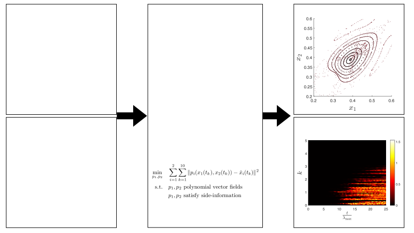
Figure 1: Schematic of the SIAR approach to the task of identifying the RD of a $0.25$-perturbed RPS game (top-left). The trajectories of the system are visualized in a Poincaré section (bottom-left). The SIAR objective is based on $10$ samples of a single trajectory of RD, and the side-information available; the forward invariance of the state space, and PC property (center). The solution of the SIAR is visualized in the same Poincaré section as the original system (top-right). The approximation error of each of the depicted trajectories with respect to Lyapunov time of the original system is depicted in the bottom-right.

Our work proposes a theoretical and computational framework for discovering the learning dynamics in a strategic multi-agent system that operates in real-time and can handle limited data. Our framework builds on recent advances in shape-constrained regression and sum-of-squares optimization [10, 11]. To identify agent dynamics, we use polynomial regression. However, to overcome the challenge of limited data, we incorporate side-information constraints that capture fundamental assumptions or expectations about agent behavior. These constraints are enforced computationally using sum-of-squares optimization.

In a strategic multi-agent system the behavior of the $i$-th agent is described by a probability distribution $x_{i}(t)$ over the available actions ${\mathcal{A}}_{i}$. If each agent is using distribution $x_{i}(t)$, the state of the system is $x(t)\equiv(x_{1}(t),\ldots,x_{n}(t))$ and the state space is the Cartesian product of simplices ${\mathcal{X}}\equiv\prod_{i=1}^{n}\mathbf{\Delta}({\mathcal{A}}_{i})$. The expected utility of agent $i$ in system state $x\in{\mathcal{X}}$ is given by the multilinear utility function $u_{i}:{\mathcal{X}}\to\mathbb{R}$ given by

$$u_{i}(x)=\sum_{a_{i}\in{\mathcal{A}}_{i}}\dotsb\sum_{a_{n}\in{\mathcal{A}}_{n}}\prod_{i=1}^{n}x_{ia_{i}}u_{i}(a_{1},\,\dotsc,\,a_{n}),$$ (1)

where $u_{i}(a_{1},\,\dotsc,\,a_{n})$ is the utility of the $i$-th agent with respect to the pure strategy-profile $(a_{1},\,\dotsc,\,a_{n})$. The evolution of an agent’s behavior is determined by its learning dynamics, which dictate how the agent updates its probability distributions over time based on the utilities it experiences. Specifically, the evolution of agent $i$ is subject to continuous-time, autonomous, and time-invariant learning dynamics $f_{i}$, i.e., $\frac{d}{dt}x_{i}(t)=f_{i}(x_{1}(t),\,\dotsc,\,x_{n}(t))$. Coupling the dynamics of the individual agents we get a dynamical system

$$\frac{d}{dt}x(t)=f(x(t))$$ (2)

describing the evolution of the state $x=(x_{1},\ldots,x_{n})\in{\mathcal{X}}$.

Our goal is to identify the ground truth vector fields $f_{1},\,\dotsc,\,f_{n}$ that describe the agents’ learning dynamics, using a constant number of $K$ noisy observations from a short run of a single system trajectory $x(t_{1}),\,\dotsc,\,x(t_{K})$, i.e., $t_{k}=(k-1)\Delta t$, $k=1,\,\dotsc,\,K$ with $\Delta t\approx 0$, and approximations of the corresponding velocities, which we denote by $\dot{x}(t_{1}),\,\dotsc,\,\dot{x}(t_{K})$. To achieve this, for each agent $i$, we approximate the true vector field $f_{i}$ by a polynomial vector field $p_{i}$. Moreover, to compensate for the absence of data we identify side-information constraints, i.e., properties that can be reasonably expected to be satisfied along the system’s trajectories. In the SIAR problem we search for polynomial regressors $p_{1},\ldots,p_{n}$ that satisfy the side-information constraints and minimize the mean square error with respect to the observational data, i.e.,

$$\underset{p_{1},\,\dotsc,\,p_{n}missing}{\text{min}} \sum_{i=1}^{n}\sum_{k=1}^{K}\|p_{i}(x(t_{k}))-\dot{x}_{i}(t_{k}))\|^{2}$$ (*SIAR)

s.t. $$p_{i} x$$ polynomial vector field in

$$\text{$p_{i}$ satisfies side-information constraints}.$$

The SIAR problem is in general computationally intractable. However, assuming that the side-information constraints can be algebraically expressed as the non-negativity or equality of (a polynomial function of) the ground truth dynamics over the state space, we can use the SOS optimization framework to obtain a hierarchy of increasingly better approximations to the true agent dynamics. The approach applied to a chaotic system is summarized in Figure 1.

2.1 Side-Information Constraints

What are the different types of side-information constraints that we can identify on the ground truth learning dynamics of the agents? Side-information constraints can be classified into two types: those that capture the geometric properties of the learning dynamics, independent of the game, and those that express assumptions or desiderata about agent behavior specific to the underlying game.

The most natural side-information constraint is that the state space ${\mathcal{X}}$ is forward-invariant, i.e., for any initialization $x(0)\in{\mathcal{X}}$ we have that $x(t)\in{\mathcal{X}}$ for all $t\geq 0$. Beyond geometric properties, various traits of agents’ behavior can be modeled by side-information constraints. One example is the positive correlation property [12, 13]:

$$\frac{d}{dt}u_{i}(x_{i}(t),x_{-i})\geq 0.$$ (*PC)

which captures the idea that an agent will choose an action that instantaneously increases their expected utility, assuming all other agents do not change their current behavior. This property encodes the agents are behaviorally rational and try to maximize their payoff. More complex trends capturing learning dynamics that trade-off exploitation in favor of exploring the possible outcomes can be also be modeled by generalizing the PC property by introducing a convex regularizer.

Another natural behavioral trait of agents is their tendency to disregard actions that are strictly dominated by alternatives. An action $a_{i}\in{\mathcal{A}}_{i}$ is strictly dominated if for any state $x\in{\mathcal{X}}$, there exists $x^{\prime}_{i}\in\Delta({\mathcal{A}}_{i})$ such that $u_{i}(x^{\prime}_{i},x_{-i})>u_{i}(e^{a_{i}},x_{-i})$. Therefore, in repeated play, it is reasonable to expect that the probability of an agent choosing a strictly dominated action eventually vanishes, i.e.,

$$\lim_{t\to+\infty}x_{ia_{i}}(t)=0,\ \;\text{ if $a_{i}$ is strictly dominated}.$$ (3)

Side-information constraints can be used to model the fact that symmetries of the underlying game, which capture that agents or actions are in some way interchangeable, should also be reflected in the agents’ dynamics [14]. As a concrete example, in a game where agents are anonymous [15], i.e., agents have the same set of actions and utility functions that are invariant under permutations of the players, we would expect the agents’ learning dynamics to also exhibit this symmetry.

Although most side-information constraints discussed earlier require knowledge of the utility functions, additional knowledge about the system can help us identify and incorporate further constraints that capture important properties of the underlying game. One example of such a constraint is Nash stationarity, which requires the Nash equilibria of the game to be fixed points of the learning dynamics. However, identifying Nash equilibria is typically intractable [16]. Another interesting property that can be used as a side-information constraint arises in potential games, where a function $V(x)$ captures unilateral deviations of agents. A reasonable assumption in this setting is that the potential function is non-decreasing along the trajectories of the learning dynamics, i.e., $\frac{d}{dt}V(x)\geq 0$.

2.2 Enforcing the Side-Information Constraints

How do we restrict the search space of the *SIAR problem to polynomial regressors $p_{i}(x)$ that satisfy the desired side-information constraints? To achieve this we rely on a cornerstone result in modern convex optimization, which allows us to efficiently search for polynomials that are nonnegative over a semi-algebraic set defined by polynomial inequalities and equality constraints $\mathcal{S}=\{x\in\mathbb{R}^{d}\mid g_{i}(x)\geq 0,h_{j}(x)=0\}$, e.g., [17, 18, 19, 20, 21, 22]. Specifically, we can use semidefinite programming to efficiently search for a fixed-degree polynomial $p(x)$, as well as fixed-degree polynomials $\sigma_{i}(x)$ and $\lambda_{j}(x)$, that satisfy the Putinar-type decomposition:

$$p(x)=\sigma_{0}(x)+\sum_{\smash{i}}\sigma_{i}(x)g_{i}(x)+\sum_{j}\lambda_{j}(x)h_{j}(x),$$ (4)

where the $\sigma_{i}(x)$’s are SOS, i.e., they can be expressed as $\sigma_{i}(x)=\sum_{k}g^{2}_{ik}(x)$. Clearly, the existence of a Putinar-type decomposition is a sufficient condition for the non-negativity of the polynomial $p(x)$ over the semi-algebraic set $\mathcal{S}$, and it necessary under additional mild assumptions [22, Theorem 3.20].

As an example, suppose we want to find polynomial regressors $p_{i}(x)$ that are forward invariant. It is a well-known fact [23] that this is equivalent to $p_{i}(x)$ lying in the tangent cone of ${\mathcal{X}}_{i}$ at the point $x_{i}$, which can be expressed as follows:

$$\sum_{a_{i}\in{\mathcal{A}}_{i}}p_{ia_{i}}(x)=0$$ (5)

$$p_{ia_{i}}(x)\geq 0\;\text{when $x_{ia_{i}}=0$}.$$

As a second example, suppose we search for polynomial regressors $p_{i}(x)$ that satisfy the positive correlation constraint. To achieve this we differentiate (*PC) and rewrite it as $\langle\nabla_{x_{i}}u_{i}(x),\,p_{i}(x)\rangle\geq 0$ for all $x\in{\mathcal{X}}$.

In either case, the desired constraint boils down to the non-negativity of a polynomial over the state space, so it can be enforced using sum-of-squares optimization. To illustrate this approach, we explain how to find a polynomial regressor that satisfies the positive correlation property for the $i$-th agent. For this, we search in the *SIAR problem for a fixed-degree polynomial $p_{i}(x)$, as well as fixed-degree polynomials $\sigma_{ia_{i}}(x)$ and $\lambda_{j}(x)$, that satisfy the Putinar-type decomposition:

$$\begin{split}\langle\nabla_{x_{i}}u_{i}(x),\,p_{i}(x)\rangle&=\sigma_{0}(x)+\sum_{i=1}^{n}\sum_{a_{i}\in{\mathcal{A}}_{i}}\sigma_{ia_{i}}(x)x_{ia_{i}}\\ &\quad+\sum_{i=1}^{n}\lambda_{i}(x)\Big{(}1-\sum_{a_{i}\in{\mathcal{A}}_{i}}x_{ia_{i}}\Big{)},\end{split}$$ (6)

where the $\sigma_{ia_{i}}$’s are SOS polynomials. For every fixed degree, we get a distinct problem, resulting in a hierarchy of increasingly better approximations to the value of *SIAR.

However, it is unclear whether this approach can give good results for two reasons. Firstly, we are attempting to approximate a potentially non-polynomial ground truth vector field using a polynomial one. Secondly, we are relaxing the polynomial non-negativity constraints expressing the side-information constraints using Putinar-type certificates. Despite these challenges, a recent result in [11], slightly extended to account for side-information constraints that express the positive correlation property (*PC) guarantees that for any time horizon $T$, approximation error $\epsilon>0$ and side-information accuracy $\delta>0$ there exists a polynomial vector field $p$ that is “$\epsilon$-close” to the ground truth dynamics (up to time $T$) and “$\delta$-satisfies” the side-information constraints. Moreover, under a mild assumption on the underlying semi-algebraic sets, the $\delta$-satisfiability of all side-information constraints admits a Putinar-type certificate.

Although the known bounds on the degree of the required certificates are exponential [22], important polynomial learning dynamics such as the RD satisfy the side-information constraints by some low-degree certificate.

3 Computational Evaluation

We evaluate the performance of our framework in various classes of games (zero-sum, anti-coordination) across various benchmarks (recovery of phase plots, recovery of support, equilibrium selection) and for various ground truth dynamics (polynomial, rational, and non-polynomial).

In our experiments we use three important learning dynamics. The first one are the replicator dynamics (RD), one of the most well-studied learning dynamics that has its roots in evolutionary game theory [24, 25]. The RD are a defined by a polynomial vector field:

$$\frac{d}{dt}x_{ia_{i}}=x_{ia_{i}}(u_{i}(e^{a_{i}},x_{-i})-u_{i}(x)),\;\forall i,a_{i},$$ (7)

where $(e^{a_{i}},x_{-i})$ is the system state obtained by $x$ in which the distribution $x_{i}$ of the $i$-th player is replaced by a point mass distribution on $a_{i}\in{\mathcal{A}}_{i}$. The RD update the frequency with which each agent $i$ adopts the action $a_{i}$ proportionally to the action’s expected utility relative to the mean. The second learning dynamics we consider are known as the log-barrier dynamics [26] and are defined by a rational vector field:

$$\frac{d}{dt}x_{ia_{i}}=x_{ia_{i}}^{2}\bigg{(}u_{i}(e^{a_{i}},x_{-i})-\frac{\sum_{a_{j}\in{\mathcal{A}}_{i}}x_{ia_{j}}^{2}u_{i}(e^{a_{j}},x_{-i})}{\sum_{a_{j}\in{\mathcal{A}}_{i}}x_{ia_{j}}^{2}}\bigg{)}.$$ (8)

The third learning dynamics we consider are the (smooth) $Q$-learning dynamics [27] defined by a non-polynomial vector field:

$$\frac{d}{dt}x_{ia_{i}}=x_{ia_{i}}(u_{i}(e^{a_{i}},x_{-i})-u_{i}(x))-T\cdot x_{ia_{i}}\left(\ln(x_{ia_{i}})+E(x_{i})\right),$$ (9)

where $E(x_{i})$ is the entropy of the distribution $x_{i}$.

3.1 A *MP Game

Figure 2: The figure on the left illustrates the replicator dynamics in the matching pennies game. In the remaining pictures, we present the results of SIAR using various side-information constraints. The red points represent the observational data $x(k\Delta t)$, $k=0,\,\dotsc,\,4$ where $x(0)=(0.2,0.3)$, and $\Delta t=0.0625$. The rest of the figures, from left to right, illustate the results of SIAR with no side information, forward invariance, positive correlation, and both constraints, respectively.

Table 1: Term-by-term comparison of the ground truth dynamics $f_{1},f_{2}$ and the *SIAR regressors $p_{1},p_{2}$.

	$f_{1}$	$p_{1}$	$f_{2}$	$p_{2}$
$1$		$0.000$		$0.000$
$x_{1}$	$-2$	$-1.998$		$0.000$
$x_{2}$		$0.000$	$2$	$2.000$
$x_{1}^{2}$	$2$	$1.998$		$0.000$
$x_{1}x_{2}$	$4$	$3.997$	$-4$	$-4.000$
$x_{2}^{2}$		$0.000$	$-2$	$-2.000$
$x_{1}^{3}$		$0.000$		$0.000$
$x_{1}^{2}x_{2}$	$-4$	$-3.997$		$0.000$
$x_{1}x_{2}^{2}$		$0.000$	$4$	$4.000$
$x_{2}^{3}$		$0.000$		$0.000$

The matching pennies game is a two-player game where each agent selects a side of a coin, either heads or tails. If both coins match, the first agent wins a payoff of one, while a mismatch results in a payoff of one for the second agent. This game is a zero-sum game, meaning that one agent’s loss is the other’s gain.

As each agent has two actions, namely heads or tails, we can represent the state space equivalently as $(x_{1},x_{2})\in[0,1]\times[0,1]$, where $x_{i}\in[0,1]$ is the $i$-th agent’s probability of choosing heads. In this setting, the RD dynamics specialize to:

$$\begin{split}\frac{d}{dt}x_{1}&=f_{1}(x_{1},x_{2})=2x_{1}(1-x_{1})(2x_{2}-1)\\ \frac{d}{dt}x_{2}&=f_{2}(x_{1},x_{2})=2x_{2}(1-x_{2})(1-2x_{1}),\end{split}$$ (*RD-*MP)

for all $x_{1},x_{2}\in[0,1]$. This allows to visualize the agent’s behavior using a two-dimensional vector field, shown in Figure 2.

The goal is to identify the ground truth dynamics $f_{1}$ and $f_{2}$ using observational data that consist of a short run of a single system trajectory ($K=5$ samples), depicted in red in Figure 2. We initialize the trajectory at $x(0)=(0.2,0.3)$, and, using a fourth-order symbolic integrator, we sample the states $x(t_{k})$, where $t_{k}=(k-1)\Delta t$, $k=1,\,\dotsc,\,K$ with $\Delta t=0.0625$. We also approximate the corresponding velocities, which we denote for simplicity by $\dot{x}(t_{k})$, using (*RD-*MP), to which we add zero-mean normally distributed noise with standard deviation $\sigma=10^{-3}$.

Next, we setup the *SIAR problem to identify polynomial dynamics $p_{1}$ and $p_{2}$ that approximate the ground truth dynamics $f_{1}$ and $f_{2}$ respectively and satisfy the forward-invariance and the positive correlation property. Forward invariance of the state space is ensured by the following inequality constraints:

$$\begin{split}p_{1}(0,x_{2})&\geq 0\\ p_{1}(1,x_{2})&\leq 0\\ \end{split}\quad\begin{split}p_{2}(x_{1},0)&\geq 0\\ p_{2}(x_{1},1)&\leq 0,\end{split}$$ (*FI-*MP)

for all $x_{1},x_{2}\in[0,1]$. Additionally, the positive correlation property is ensured by the following two constraints:

$$2(2x_{2}-1)p_{1}(x_{1},x_{2}) \geq 0$$ (*PC-*MP)

$$2(1-2x_{1})p_{2}(x_{1},x_{2}) \geq 0,$$

for $x_{1},x_{2}\in[0,1]$. Summarizing, the *SIAR problem is given by:

$$\underset{p_{1},p_{2}}{\text{minimize}} \sum_{i=1}^{2}\sum_{k=1}^{K}(p_{1}(x_{1}^{(k)},x_{2}^{(k)})-\dot{x}_{i}^{(k)})^{2}$$ (10)

subject to $$p_{1}(0,x_{2})\geq 0,\ \text{for all }x_{2}\in[0,1]$$

$$p_{1}(1,x_{2})\leq 0,\ \text{for all }x_{2}\in[0,1]$$

$$p_{2}(x_{1},0)\geq 0,\ \text{for all }x_{1}\in[0,1]$$

$$p_{2}(x_{1},1)\leq 0,\ \text{for all }x_{1}\in[0,1]$$

$$2(2x_{2}-1)p_{1}(x_{1},x_{2})\geq 0,\ \text{for all }x_{1},x_{2}\in[0,1]$$

$$2(1-2x_{1})p_{2}(x_{1},x_{2})\geq 0,\ \text{for all }x_{1},x_{2}\in[0,1]$$

Finally, we approximate the value of the *SIAR problem using SOS optimization. Specifically, we search for degree $d=2$ polynomials $p_{1}$ and $p_{2}$, and relax all polynomial inequality constraints by searching for a degree $4$ Putinar-type decomposition. We solve the corresponding semidefinite program using the MOSEK as the optimization software [28].Table 1 depicts the *SIAR regressors $p_{1}$ and $p_{2}$ when compared term-by-term with the ground truth dynamics in (*RD-*MP), where each term is rounded to three decimal digits.

In addition to relying solely on term-by-term comparison, which may not provide a reliable indicator of the accuracy of the method, especially in cases where the system experiences chaotic behavior, we can also visually assess the accuracy of the regressor in this example due to the system’s low dimensionality. Indeed, as depicted in Figure 2, the two systems have identical behavior for all possible inializations.

3.2 A Congestion Game with Multiple Equilibria

Table 2: Accuracy(%) of the SIAR regressor in solving the equilibrium selection problem for a congestion game with multiple equilibria

	*RD		*LBD		*QLD
$n$	$d=4$	$d=5$	$d=4$	$d=5$	$d=4$	$d=5$
$2$	$100$	$99.99$	$99.99$	$99.99$	$96.12$	$99.99$
$4$	$100$	$100$	$100$	$100$	$99.82$	$100$
$6$	$100$	$100$	$100$	$100$	$100$	$100$
$8$	$100$	$100$	$100$	$100$	$100$	$100$
$10$	$100$	$100$	$99.98$	$99.97$	$100$	$100$

A congestion game is a type of anti-coordination game where agents try to minimize their own delay while choosing a path through a network with delay functions on arcs that depend on congestion conditions. In this example, we consider the simplest possible network topology for a congestion game, where each of $n$ agents is presented with two choices of arcs ${\mathcal{A}}$ from a single origin node to a single destination node. In this context, the utility of an agent is given by the expected number of commuters that use the same arc, which directly affects the delay experienced by the agent.

Despite having only two arcs, this game has an exponential number of pure Nash equilibria as a function of the number of players, more specifically we have $O\begin{pmatrix}n\\ \frac{n}{2}\end{pmatrix}$ equilibrium points, making it challenging for players to coordinate on a specific one of them. This is known as the equilibrium selection problem in game theory. However, any AMS dynamics—a class of dynamics that includes the RD and the LBD—for a generic congestion game, converge almost surely to a deterministic Nash equilibirum of the game [29]. On the other QLD converge to states that are known as Quantal Response Equilibria, an extension of Nash equilibria, which takes into account the trade-off between exploitation and exploration of the state space that each agent naturally accepts in this setup.

Our congestion game also exemplifies the concept of anonymity in games, meaning that the delay experienced by an agent depends solely on how many other agents have chosen the same arc, and not on their individual identities. In other words, for any agent $i$ and for any permutation (relabelling), $\pi:\{1,\,\dotsc,\,n\}\to\{1,\,\dotsc,\,n\}$, of the agents we have that:

$$u_{i}(a_{1},\,\dotsc,\,a_{n})=u_{\pi(i)}(a_{\pi^{-1}(1)},\,\dotsc,\,a_{\pi^{-1}(n)}),\;\forall a_{i}\in{\mathcal{A}}.$$ (11)

As a result, it is reasonable to assume that the learning dynamics $f_{i}$ employed by the agents also inherit this symmetry. That is, for any agent $i$ and any permutation $\pi$:

$$f_{i}(x_{1},\ldots,x_{n})=f_{\pi(i)}(x_{\pi^{-1}(1)},\,\dotsc,\,x_{\pi^{-1}(n)}),\;\forall x\in{\mathcal{X}}.$$ (12)

Next, we setup the *SIAR problem to identify polynomial dynamics $p_{i}$ that approximate the true dynamics $f_{i}$ for all agents $i=1,\dots,n$. Besides the forward-invariance of the state-space and the positive correlation property, we also impose as a side-information constraint the symmetry on the learning dynamics given in (12), induced by the agent anonymity.

In order to evaluate the effectiveness of the SIAR framework, we conduct three sets of experiments with different ground truth dynamics: the replicator, the log-barrier, and the $Q$-learning dynamics. In each individual test we recompute the SIAR regressor using a short run of a trajectory with an initial random state $x(0)\in[0,1]^{n}$. Finally, we approximate the value of the SIAR problem using SOS optimization. Specifically, we search for degree $d$ polynomials $p_{1},\ldots,p_{n}$ and relax all polynomial inequality constraints by Putinar-type decompositions. For $10^{3}$ random intializations we simulate both the ground truth dynamics and the SIAR regressor (for an appropriately long window of time) and check whether they converge to the same equlibrium point. We perform $10$ independent tests for each ground truth dynamics, with $n=2,4,6,8,10$ and $d=4,5$, and report the average probability that both SIAR and the true dynamics converge to the same equilibrium. For both polynomial (replicator) and rational (log-barrier) dynamics, we achieve near-perfect recovery. For non-polynomial dynamics, the accuracy improves rapidly as the degree of the regressor increases, see Table 2.

Chaotic dynamics in a RPS game

Figure 3: The Poincaré maps of $10$ differente trajectories of the *RD (left), and the *SIAR problem’s solution (right) in a $0.25$-perturbed *RPS game with respect to the Poincaré section $\{x\in{\mathcal{X}}\,:\,x_{ia_{1}}-x_{ia_{2}}=0\;\forall i=1,\,2\}$. Each trajectory $k$ is initialized at $x^{(k)}_{1}(0)=(0.5,0.025k,0.5-0.025k)$ where $k=1,\,\dotsc,\,10$ and $x_{2}(0)=(0.5,0.25,0.25)$.

Table 3: The payoff matrix of an $\epsilon$-pertubed *RPS game.

Figure 4: The error of the *SIAR problem’s solution for the trajectories $x_{k}(t)$, $k=1,\,\dotsc,\,10$, initialized at $x^{(k)}_{1}(0)=(0.5,0.025k,0.5-0.025k)$ and $x_{2}(0)=(0.5,0.25,0.25)$.

Finally, we consider the case of an $\epsilon$-perturbed RPS game, a two-player zero-sum game given by the payoff matrix in Table 3.

The $\epsilon$-perturbed RPS game is based on a classic RPS game, but ties between the two players are broken slightly in favor of the first player. Specifically, while any winning combination gives the winning player utility $1$, and the losing player utility $-1$, ties yield utility $\epsilon$ to the first player, and $-\epsilon$ to the second player, where $-1<\epsilon<1$.

In our third computational study, we consider the replicator dynamics in the $\epsilon$-perturbed RPS game, which is known to exhibit chaotic behavior [30]. Informally, this means that a slight estimation error in the system’s state leads to radically different trajectories as time evolves. Furthermore, those trajectories, at times, may come arbitrarily close and move arbitrarily apart.

This six-dimensional system can be visualized through its Poincaré sections, which are defined as the set of points where multiple trajectories intersect a two-dimensional affine space. In Figure 3 (left) we depict the Poincaré sections of the replicator dynamics in a $0.25$-RPS game of $10$ different trajectories initialized at $x^{(k)}_{1}(0)=(0.5,0.025k,0.5-0.025k)$ where $k=1,\,\dotsc,\,10$ and $x_{2}(0)=(0.5,0.25,0.25)$ with respect to two-dimensional affine subspace:

$$\{x\in\mathbb{R}^{6}\,:\,x_{ia_{1}}-x_{ia_{2}}=0,\sum_{a_{i}\in{\mathcal{A}}}x_{ia_{i}}=1,\;\forall i=1,\,2\}$$ (13)

Trajectories corresponding to higher values of $k$ (black points in Figure 3, left) tend to follow a regular, almost circular pattern on the Poincaré section. In contrast, trajectories corresponding to lower values of $k$ (red points in Figure 3, left) are more spread out and less predictable.

To identify polynomial dynamics that can approximate the true replicator dynamics, we set up the *SIAR problem using a dataset of $10$ samples from a short run single system trajectory. To enhance the accuracy of the approximation, we incorporate forward invariance and positive correlation as side-information constraints. Finally, to solve the SIAR problem, we use SOS optimization to search for degree 3 polynomial vector fields, relaxing all polynomial inequality constraints by looking for a Putinar-type decomposition.

In Figure 3, we plot the same Poincaré section with respect to the ground truth replicator dynamics (left) and the SIAR regressor (right). Despite the underlying replicator dynamics being chaotic, we observe that the SIAR regressor approximates trajectories corresponding to higher values of $k$ very well. Furthermore for trajectories corresponding to lower values of $k$ where the trajectories of the replicator dynamics are more scrambled, this behavior is also captured by the trajectories of the SIAR regressor.

Finally, in Figure 4 we plot the error with respect to the $L_{\infty}$-norm between the SIAR regressor and the actual trajectories $x_{k}(t)$. Our experiment reveal that estimation the error is very small in magnitude ($\leq 10^{-3}$) for at least $8$ Lyapunov times, with the accuracy increasing significantly for trajectories with less radical behaviori.e., larger values of $k$. The Lyapunov exponent is a quantity that characterizes the rate of separation of infinitesimally close trajectories, i.e.,

$$\lambda_{\max}=\max_{\begin{subarray}{c}i\in\{1,\,\dotsc,\,n\}\\ a_{i}\in{\mathcal{A}}_{i}\end{subarray}}\lim_{t\to\infty}\lim_{\delta\to 0}\frac{1}{t}\ln\frac{\lvert x_{ia_{i}}(t)-x^{\prime}_{ia_{i}}(t)\rvert}{\delta},$$ (14)

where $\delta\equiv\lvert x_{ia_{i}}(0)-x^{\prime}_{ia_{i}}(0)\rvert$ is the initial separation of the two trajectories direction $e^{ia_{i}}$. The inverse of the Lyapunov exponent is known as Lyapunov time and is the minimum time required for infinitesimal initialization error to grow by a factor of $e$.

Appendix A *SIAR: Overview

In a strategic multi-agent system, each agent’s behavior can be modeled by a probability distribution $x_{i}(t)$ over the available actions ${\mathcal{A}}_{i}$. The state of the system at time $t$ is then given by $x(t)=(x_{1}(t),\dots,x_{n}(t))$, and the state space is the Cartesian product of simplices ${\mathcal{X}}=\prod_{i=1}^{n}\mathbf{\Delta}({\mathcal{A}}_{i})$. The expected utility of agent $i$ in a given system state $x\in{\mathcal{X}}$ is defined by a multilinear utility function $u_{i}:{\mathcal{X}}\to\mathbb{R}$, which is calculated by multiplying the probabilities of the actions chosen by each agent in $x$ and then summing over all possible action profiles $(a_{1},\dots,a_{n})\in\prod_{i=1}^{n}{\mathcal{A}}_{i}$:

$$u_{i}(x)=\sum_{a_{i}\in{\mathcal{A}}_{i}}\dotsb\sum_{a_{n}\in{\mathcal{A}}_{n}}\prod_{i=1}^{n}x_{ia_{i}}u_{i}(a_{1},\,\dotsc,\,a_{n}).$$ (15)

The evolution of an agent’s behavior over time is governed by its learning dynamics, which update the agent’s probability distribution based on the utilities it receives. Specifically, the dynamics of agent $i$ are given by $\frac{d}{dt}x_{i}(t)=f_{i}(x_{1}(t),\,\dotsc,\,x_{n}(t))$. By coupling the dynamics of all agents together, we obtain the dynamical system:

$$\frac{d}{dt}x(t)=f(x(t)),$$ (16)

which describes the evolution of the state $x=(x_{1},\dots,x_{n})$ over time.

Our goal is to identify the ground truth vector fields $f_{1},\,\dotsc,\,f_{n}$ that describe the agents’ learning dynamics, using a constant number of $K$ noisy observations from a short run of a single system trajectory $x(t_{1}),\,\dotsc,\,x(t_{K})$, i.e., $t_{k}=(k-1)\Delta t$, $k=1,\,\dotsc,\,K$ with $\Delta t\approx 0$, and approximations of the corresponding velocities, which we denote by $\dot{x}(t_{1}),\,\dotsc,\,\dot{x}(t_{K})$. To achieve this, for each agent $i$, we approximate the true vector field $f_{i}$ by a polynomial vector field $p_{i}$. Moreover, to compensate for the absence of data we identify side-information constraints that capture fundamental assumptions or expectations about agent behavior. In the SIAR problem we search for polynomial regressors $p_{1},\dots,p_{n}$ that satisfy the side-information constraints and minimize the mean square error with respect to the observational data, i.e.,

$$\underset{p_{1},\,\dotsc,\,p_{n}missing}{\text{min}} \sum_{i=1}^{n}\sum_{k=1}^{K}\|p_{i}(x(t_{k}))-\dot{x}_{i}(t_{k})\|^{2}$$ (17)

s.t. $$p_{i} x$$ polynomial vector field in

$$\text{$p_{i}$ satisfies side-information constraints}.$$

The SIAR problem is in general computationally intractable. However, assuming that the side-information constraints can be algebraically expressed as the non-negativity or equality of (a polynomial function of) the ground truth dynamics over the state space, we can use the SOS optimization framework to obtain a hierarchy of increasingly better approximations to the true agent dynamics.

A.1 Side-Information Constraints

In this section, we aim to outline the side-information constraints that have been employed in our work. These constraints are based on the natural properties of the learning dynamics utilized by the agents in the multi-agent system being studied. The identified side-information constraints encompass a range of factors, including geometric properties of the dynamics, game-specific characteristics, and behavioral aspects of the agents

One of the most natural side-information constraints in our work is the forward-invariance of the state space ${\mathcal{X}}$. This constraint ensures that for any initialization $x(0)\in{\mathcal{X}}$, the state remains in ${\mathcal{X}}$ for all $t\geq 0$. In terms of dynamics, this means that $f(x)$ is a direction that can be infinitesimally traversed from $x$ without leaving the state space. Mathematically, this implies that the direction $f(x)$ lies in the tangent cone of ${\mathcal{X}}$ at point $x$ [23], represented by the following algebraic constraints:

$$\sum_{a_{i}\in{\mathcal{A}}_{i}}f_{ia_{i}}(x) =0,\;\forall i$$ (18)

$$f_{ia_{i}}(x) \geq 0,\;\text{whenever $x_{ia_{i}}=0$}\;\forall,i,a_{i}\in{\mathcal{A}}_{i}.$$

A closely related property, widely applicable in evolutionary game theory, is that populations that start off with zero frequency $x_{ia_{i}}(0)=0$, they remain at level zero for all time, i.e., $x_{ia_{i}}(t)=0$ for all $t\geq 0$. In terms of the dynamics, this means that the faces of the state space ${\mathcal{X}}$ are forward-invariant.

In addition to geometric properties, side-information constraints can also model various behavioral traits of agents. One such example is the positive correlation property [12, 13], which is captured by the inequality:

$$\frac{d}{dt}u_{i}(x_{i}(t),x_{-i})\geq 0,$$ (19)

which reflects the idea that an agent will select an action that instantaneously does not decrease their expected utility, assuming all other agents maintain their current behavior. More complex, such as learning dynamics which involve balancing the trade-off between exploitation and exploration of system’s states, can be modeled by generalizing the positive correlation property using a convex regularizer.

Side-information constraints can also be used to model the fact that symmetries of the underlying game, which capture that agents or actions are in some way interchangeable, should also be reflected in the agents’ dynamics [14]. As a concrete example, in a game where agents are anonymous [15], i.e., agents have the same set of actions and utility functions that are invariant under permutations of the players, we would expect the agents’ learning dynamics to also exhibit this symmetry. As a concrete example, a congestion game exemplifies the concept of anonymity in games, meaning that the delay experienced by an agent depends solely on how many other agents have chosen the same arc, and not on their individual identities. In other words, for any agent $i$ and for any permutation (relabelling), $\pi:\{1,\,\dotsc,\,n\}\to\{1,\,\dotsc,\,n\}$, of the agents we have that:

$$u_{\pi(i)}(a_{\pi^{-1}(1)},\,\dotsc,\,a_{\pi^{-1}(n)})=u_{i}(a_{1},\,\dotsc,\,a_{n}),\;\text{for all $a_{i}\in{\mathcal{A}}$}.$$ (20)

More generally, in terms of mixed strategies, anonymity implies that for any bijection ${\pi}:{\mathcal{N}}\to{\mathcal{N}}$:

$$u_{\pi(i)}(x_{\pi^{-1}(1)},\dots,x_{\pi^{-1}(n)})={u}_{i}(x_{1},\dots,x_{n}),\;\text{for all ${i}\in{\mathcal{N}}$, and ${x}\in{\mathcal{X}}$}.$$ (21)

Indeed, for any bijection ${\pi}:{\mathcal{N}}\to{\mathcal{N}}$ we have that

$$u_{i}(x) =\sum_{a_{1},\dots,a_{n}\in{\mathcal{A}}}x_{1a_{1}}\dots x_{na_{n}}u_{i}(a_{1},\dots,a_{n})$$ (22)

$$=\sum_{a_{1},\dots,a_{n}\in{\mathcal{A}}}x_{1a_{1}}\dots x_{na_{n}}u_{\pi(i)}(a_{\pi^{-1}(1)},\dots,a_{\pi^{-1}(n)})$$

$$=\sum_{a_{1},\dots,a_{n}\in{\mathcal{A}}}x_{\pi^{-1}(1)a_{\pi^{-1}(1)}}\dots x_{\pi^{-1}(n)a_{\pi^{-1}(n)}}u_{\pi(i)}(a_{\pi^{-1}(1)},\dots,a_{\pi^{-1}(n)})$$

$$=u_{\pi(i)}(\pi^{-1}(x)).$$

When playing an anonymous game, it is reasonable to assume that the learning dynamics $f_{i}$ employed by the agents exhibit the same symmetry. In other words, for any agent $i$ and any permutation $\pi$

$$f_{i}(x_{1},\dots,x_{n})=f_{\pi(i)}(x_{\pi^{-1}(1)},\,\dotsc,\,x_{\pi^{-1}(n)}),\;\text{for all $x\in{\mathcal{X}}$}.$$ (23)

Another natural behavioral trait of agents is their tendency to disregard actions that are strictly dominated by alternatives. An action $a_{i}\in{\mathcal{A}}_{i}$ is strictly dominated if for any state $x\in{\mathcal{X}}$, there exists $x^{\prime}_{i}\in\Delta({\mathcal{A}}_{i})$ such that $u_{i}(x^{\prime}_{i},x_{-i})>u_{i}(e^{a_{i}},x_{-i})$. Therefore, in repeated play, it is reasonable to expect that the probability of an agent choosing a strictly dominated action eventually vanishes, i.e.,

$$\lim_{t\to+\infty}x_{ia_{i}}(t)=0,\;\text{if $a_{i}$ is strictly dominated}.$$ (24)

The property of eliminating dominated strategies can be defined recursively by considering sub-games of the original game where dominated strategies have been eliminated. The rationale behind this recursion lies in the fact that if an action $a_{i}\in{\mathcal{A}}_{i}$ of some player $i$ is strictly dominated, and the other agents are aware that the $i$-th agent will eventually avoid this action, they can act strategically upon this fact. On way to enforce the elimination of dominated strategies, is to focus on a special class of learning dynamics called RSD that have the form

$$\frac{d}{dt}x_{ia_{i}}=x_{ia_{i}}g_{ia_{i}}(x),\;\text{for all $x\in{\mathcal{X}}$},$$ (25)

where $g_{ia_{i}}(x)$ has an open domain, is locally Lipschitz continuous, and satisfies $\sum_{a_{i}\in{\mathcal{A}}_{i}}x_{ia_{i}}g_{ia_{i}}(x)=0$ for all agents $i$. A classical result in evolutionary game theory states that any RSD dynamics that satisfies convex monotonicity, i.e.,

$$\forall a_{i},\tilde{x}_{i}:\;\text{if ${u}_{i}(\tilde{{x}}_{i},{x}_{-{i}})>{u}_{i}({e}^{{{a}_{{i}}}},{x}_{-{i}})$ then $\big{\langle}\tilde{{x}}_{i},\,{{g}^{\mathrm{\acs*{RD}}}_{i}}({x})\big{\rangle}>{{g}^{\mathrm{\acs*{RD}}}_{{i}{{a}_{{i}}}}}({x})$ for all ${x}\in{\mathcal{X}}$}.$$ (26)

asymptotically leads to the elimination of any strictly dominated actions of a normal-form game (see [31]).

A.2 The 2-Player Case: A Compact Reformulation

In some of the examples studied in this work, each of the $n$ agents faces a binary choice between two actions ${\mathcal{A}}_{i}$. The standard description of the state space for such a system requires $2n$ variables $x_{ia_{i}}$ and $2n$ functions $f_{ia_{i}}$ describing the evolution of the state space ${\mathcal{X}}$. However, as we explain below, such a system can be equivalently represented using a single variable $x_{i}\in[0,1]$ for each agent and a single vector field $f_{i}(x)$ acting on the reduced state space $x=(x_{1},\dots,x_{n})\in[0,1]^{n}$. Specifically, the reduced state space is given by $[0,1]^{{n}}$ where each state ${x}=(x_{1},\dots,x_{n})$ specifies the probabilities of the agents choosing their first action. The probability of choosing the second action is $x_{ia_{2}}=1-x_{ia_{1}}$ and its evolution is given by:

$$\frac{d}{d\,{t}}x_{ia_{2}}(t)=\frac{d}{d\,{t}}(1-x_{ia_{1}}(t))=-\frac{d}{dt}x_{ia_{1}}(t)=-f_{ia_{1}}(x(t)),\;\text{for each ${x}\in[0,1]^{{n}}$}.$$ (27)

Consequently, the evolution of each agent is described by a single function:

$$f_{i}(x)\equiv f_{ia_{1}}(x)=-f_{ia_{2}}(x),\;\text{for all $i\in{\mathcal{N}},x\in[0,1]^{{n}}$}.$$ (28)

As a concrete example, the replicator dynamics with two strategies for each agent are given by:

$$\dot{x}_{ia_{1}} =x_{ia_{1}}(u_{i}(a_{i1},x_{-i})-u_{i}(x))$$ (29)

$$=x_{ia_{1}}\Big{(}u_{i}(a_{i1},x_{-i})-(x_{ia_{1}}u_{i}(a_{i1},x_{-i})+(1-x_{ia_{1}})u_{i}(a_{i2},x_{-i})\Big{)}$$

$$=x_{ia_{1}}\Big{(}(1-x_{ia_{1}})u_{i}(a_{i1},x_{-i})-(1-x_{ia_{1}})u_{i}(a_{i2},x_{-i})\Big{)}$$

$$=x_{ia_{1}}(1-x_{ia_{1}})\Big{(}u_{i}(a_{i1},x_{-i})-u_{i}(a_{i2},x_{-i})\Big{)}.$$

Recalling that $x_{i}=x_{ia_{1}}$, the replicator dynamics in this case can be rewritten as:

$$\dot{x}_{i}=x_{i}(1-x_{i})\Big{(}u_{i}(a_{i1},x_{-i})-u_{i}(a_{i2},x_{-i})\Big{)}.$$ (30)

When using the reduced description of the system over $[0,1]^{n}$, the form of the side-information constraints also changes accordingly and can be expressed solely in terms of $f_{i}(x)$. We explain this below for the forward invariance and the positive correlation properties. As agents have only two strategies, forward invariance boils down to:

$$f_{ia_{1}}(x)+f_{ia_{2}}(x)=0$$ (31a)

$$f_{ia_{i}}(x)\geq 0\;\text{when $x_{ia_{i}}=0$}.$$ (31b)

Recalling (28), the first constraint in (31a) is always satisfied, and the constraint in (31b) becomes

$$f_{ia_{1}}(x)\geq 0\;\text{when $x_{ia_{1}}=0$}$$ (32a)

$$f_{ia_{2}}(x)\geq 0\;\text{when $x_{ia_{2}}=0$}.$$ (32b)

Finally, over the reduced space, and recalling that $x_{i}=x_{ia_{1}}$ and $f_{i}(x)=f_{ia_{1}}(x)=-f_{ia_{2}}(x)$, (32) is equivalent to:

$${f}_{i}({x})\geq 0\;\text{whenever ${x}_{i}=0$}$$ (33a)

$$- {f}_{i}({x})\geq 0\;\text{whenever ${x}_{i}=1$},$$ (33b)

for all agents ${i}\in{\mathcal{N}}$, and for all ${x}\in[0,1]^{n}$. Summarizing, forward invariance of the state space can be written compactly as:

$${f}_{i}(0,{x}_{-{i}})\geq 0\quad\text{and}\quad{f}_{i}(1,{x}_{-{i}})\leq 0,\;\text{ for all ${i}\in{\mathcal{N}}$ and $x\in[0,1]^{n}$}.$$ (34)

Next, we consider the case of the positive correlation constraint, given by the inequality:

$$\frac{d}{d\,t}{u}_{i}({x}_{i}(t),{x}_{-{i}})=\sum_{{{a}_{{i}}}\in{\mathcal{A}}_{i}}\frac{\partial{u}_{i}({x})}{\partial{x}_{{i}{{a}_{{i}}}}}f_{ia_{i}}(x)=\sum_{{{a}_{{i}}}\in{\mathcal{A}}_{i}}u_{i}(e^{a_{i}},x_{-i})f_{ia_{i}}(x)\geq 0,$$ (35)

where for the second equality we used (31b). In the case where each agent has two strategies, this becomes:

$$u_{i}(e^{a_{i1}},x_{-i})f_{ia_{1}}(x)+u_{i}(e^{a_{i2}},x_{-i})f_{ia_{2}}(x)\geq 0$$ (36)

Finally, using that (28) this can be rewritten as

$$(u_{i}(e^{a_{i1}},x_{-i})-u_{i}(e^{a_{i2}},x_{-i}))f_{i}(x)\geq 0,\;\text{for all $x\in[0,1]^{n}$}.$$ (37)

Appendix B Properties of Various Learning Dynamics

B.1 The *RD

In this section we show that the RD given by:

$$\dot{x}_{{i}{{a}_{{i}}}}={{f}^{\mathrm{\acs*{RD}}}_{{i}{{a}_{{i}}}}}({x})\triangleq{x}_{{i}{{a}_{{i}}}}\big{(}{u}_{i}({e}^{{{a}_{{i}}}},{x}_{-{i}})-{u}_{i}({x})\big{)},\;\text{for all ${i}\in{\mathcal{N}}$, ${{a}_{{i}}}\in{\mathcal{A}}_{i}$, and ${x}\in{\mathcal{X}}$},$$ (38)

satisfy a series of side-information constraints, namely, the forward-invariance of the faces of the state space ${\mathcal{X}}$,(cf. 1) the PC property (cf. 2), the agent anonymity property (cf. 4), and they asymptotically lead to the elimination of strictly dominated actions (cf. 3).

Proposition 1.

The faces of the state space ${\mathcal{X}}$ (and thus, also the state space itself) are forward-invariant with respect to the replicator dynamics, i.e., the following equalities hold:

$$\sum_{{{a}_{{i}}}\in{\mathcal{A}}_{i}}{{f}^{\mathrm{\acs*{RD}}}_{{i}{{a}_{{i}}}}}({x}) =0,\;\text{for all ${i}\in{\mathcal{N}}$, and ${x}\in{\mathcal{X}}$},$$ (39a)

$${{f}^{\mathrm{\acs*{RD}}}_{{i}{{a}_{{i}}}}}({x}) \geq 0,\;\text{whenever ${x}_{{i}{{a}_{{i}}}}=0$, for all ${i}\in{\mathcal{N}}$, ${{a}_{{i}}}\in{\mathcal{A}}_{i}$, and ${x}\in{\mathcal{X}}$}.$$ (39b)

Proof.

(39b) is a trivial implication of the definition of ${{f}^{\mathrm{\acs*{RD}}}_{{i}{{a}_{{i}}}}}({x})$. To prove (39a), let ${i}\in{\mathcal{N}}$ be an arbitrary agent, and let ${x}\in{\mathcal{X}}$ be an arbitrary system state, and observe that:

$$\sum_{{{a}_{{i}}}\in{\mathcal{A}}_{i}}{{f}^{\mathrm{\acs*{RD}}}_{{i}{{a}_{{i}}}}}({x}) =\sum_{{{a}_{{i}}}\in{\mathcal{A}}_{i}}{x}_{{i}{{a}_{{i}}}}\big{(}{u}_{i}({e}^{{{a}_{{i}}}},{x}_{-{i}})-{u}_{i}({x})\big{)}$$ (40a)

$$=\sum_{{{a}_{{i}}}\in{\mathcal{A}}_{i}}{x}_{{i}{{a}_{{i}}}}{u}_{i}({e}^{{{a}_{{i}}}},{x}_{-{i}})-{u}_{i}({x})\sum_{{{a}_{{i}}}\in{\mathcal{A}}_{i}}{x}_{{i}{{a}_{{i}}}}$$ (40b)

$$=\sum_{{{a}_{{i}}}\in{\mathcal{A}}_{i}}{x}_{{i}{{a}_{{i}}}}{u}_{i}({e}^{{{a}_{{i}}}},{x}_{-{i}})-{u}_{i}({x})$$ (40c)

$$={u}_{i}({x})-{u}_{i}({x})$$ (40d)

$$=0.$$ (40e)

∎

Proposition 2.

The replicator dynamics satisfy the positive correlation property with a Putinar-type certificate.

Proof.

Consider an arbitrary agent ${i}\in{\mathcal{N}}$, and let ${x}\in{\mathcal{X}}$ an arbitrary system state. Since $u_{i}(x)$ is multilinear we have: $u_{i}(x)=\sum_{a_{i}\in{\mathcal{A}}_{i}}x_{ia_{i}}u_{i}(e^{a_{i}},x_{-i})$ and consequently,

$$\frac{\partial u_{i}(x)}{\partial x_{ia_{i}}}=u_{i}(e^{a_{i}},x_{-i}).$$ (41)

Finally, we have

$$\frac{d}{d\,t}{u}_{i}({x}_{i}(t),{x}_{-{i}}) =\Big{\langle}\nabla_{{x}_{i}}{u}_{i}({x}),\,{{f}^{\mathrm{\acs*{RD}}}_{i}}({x})\Big{\rangle}$$ (42a)

$$=\sum_{{{a}_{{i}}}\in{\mathcal{A}}_{i}}\frac{\partial{u}_{i}({x})}{\partial{x}_{{i}{{a}_{{i}}}}}{{f}^{\mathrm{\acs*{RD}}}_{{i}{{a}_{{i}}}}}({x})$$ (42b)

$$=\sum_{{{a}_{{i}}}\in{\mathcal{A}}_{i}}{u}_{i}({e}^{{{a}_{{i}}}},{x}_{-{i}}){{f}^{\mathrm{\acs*{RD}}}_{{i}{{a}_{{i}}}}}({x})$$ (42c)

$$=\sum_{{{a}_{{i}}}\in{\mathcal{A}}_{i}}{u}_{i}({e}^{{{a}_{{i}}}},{x}_{-{i}}){x}_{{i}{{a}_{{i}}}}\big{(}{u}_{i}({e}^{{{a}_{{i}}}},{x}_{-{i}})-{u}_{i}({x})\big{)}$$ (42d)

$$=\sum_{{{a}_{{i}}}\in{\mathcal{A}}_{i}}{x}_{{i}{{a}_{{i}}}}\big{(}{u}_{i}({e}^{{{a}_{{i}}}},{x}_{-{i}})\big{)}^{2}-{u}_{i}({x})\sum_{{{a}_{{i}}}\in{\mathcal{A}}_{i}}{x}_{{i}{{a}_{{i}}}}{u}_{i}({e}^{{{a}_{{i}}}},{x}_{-{i}})$$ (42e)

$$=\sum_{{{a}_{{i}}}\in{\mathcal{A}}_{i}}{x}_{{i}{{a}_{{i}}}}\big{(}{u}_{i}({e}^{{{a}_{{i}}}},{x}_{-{i}})\big{)}^{2}-\big{(}{u}_{i}({x})\big{)}^{2}$$ (42f)

$$=\sum_{{{a}_{{i}}}\in{\mathcal{A}}_{i}}{x}_{{i}{{a}_{{i}}}}\big{(}{u}_{i}({e}^{{{a}_{{i}}}},{x}_{-{i}})-{u}_{i}({x})\big{)}^{2}\geq 0$$ (42g)

Finally, the utilities ${u}_{i}({e}^{{{a}_{{i}}}},{x}_{-{i}})$ and ${u}_{i}({x})$ are both multi-linear polynomials. Consequently, the expression $\sum_{{{a}_{{i}}}\in{\mathcal{A}}_{i}}{x}_{{i}{{a}_{{i}}}}\big{(}{u}_{i}({e}^{{{a}_{{i}}}},{x}_{-{i}})-{u}_{i}({x})\big{)}^{2}$ is a Putinar-type certificate for the non-negativity of $\frac{d}{d\,t}{u}_{i}({x}_{i}(t),{x}_{-{i}})$ over the state space:

$${\mathcal{X}}=\Big{\{}x=(x_{ia_{i}})\,:\,x_{ia_{i}}\geq 0,\sum_{a_{i}\in{\mathcal{A}}_{i}}x_{ia_{i}}=1\Big{\}}.$$ (43)

∎

Proposition 3.

The replicator dynamics asymptotically lead to the elimination of strictly dominated actions.

Proof.

We first show that the RD are RSD (cf. §A.1). For this we rewrite (38) as:

$$\dot{x}_{{i}{{a}_{{i}}}}={x}_{{i}{{a}_{{i}}}}{{g}^{\mathrm{\acs*{RD}}}_{{i}{{a}_{{i}}}}}({x})\;\text{for all ${i}\in{\mathcal{N}}$, ${{a}_{{i}}}\in{\mathcal{A}}_{i}$, and ${x}\in{\mathcal{X}}$},$$ (44)

where the growth rate functions, ${{g}^{\mathrm{\acs*{RD}}}_{{i}{{a}_{{i}}}}}$, given by:

$${{g}^{\mathrm{\acs*{RD}}}_{{i}{{a}_{{i}}}}}({x})\triangleq{u}_{i}({e}^{{{a}_{{i}}}},{x}_{-{i}})-{u}_{i}({x}),\;\text{for all ${i}\in{\mathcal{N}}$, ${{a}_{{i}}}\in{\mathcal{A}}_{i}$, and ${x}\in\mathbb{R}^{\lvert{\mathcal{A}}_{1}\rvert}\times\dots\times\mathbb{R}^{\lvert{\mathcal{A}}_{n}\rvert}$},$$ (45)

are polynomial functions—hence, Lipschitz continuous in ${\mathcal{X}}$—and, by 1, satisfy $\sum_{{{a}_{{i}}}\in{\mathcal{A}}_{i}}{x}_{{i}{{a}_{{i}}}}{{g}^{\mathrm{\acs*{RD}}}_{{i}{{a}_{{i}}}}}({x})=0$ for all agents ${i}\in{\mathcal{N}}$, and all system states ${x}\in{\mathcal{X}}$. Finally, we have to show that RD satisfy convex monotonicity (26), i.e.,

$$\forall a_{i},\tilde{x}_{i}:\text{if ${u}_{i}(\tilde{{x}}_{i},{x}_{-{i}})>{u}_{i}({e}^{{{a}_{{i}}}},{x}_{-{i}})$ then $\big{\langle}\tilde{{x}}_{i},\,{{g}^{\mathrm{\acs*{RD}}}_{i}}({x})\big{\rangle}>{{g}^{\mathrm{\acs*{RD}}}_{{i}{{a}_{{i}}}}}({x})$ for all ${x}\in{\mathcal{X}}$ }.$$ (46)

Note that the RD dynamics satisfy:

$$\big{\langle}\tilde{{x}}_{i},\,{{g}^{\mathrm{\acs*{RD}}}_{i}}({x})\big{\rangle}-{{g}^{\mathrm{\acs*{RD}}}_{{i}{{a}_{{i}}}}}({x}) =\sum_{{\tilde{{a}}_{{i}}}\in{\mathcal{A}}_{i}}\tilde{{x}}_{{i}{\tilde{{a}}_{{i}}}}{{g}^{\mathrm{\acs*{RD}}}_{{i}{\tilde{{a}}_{{i}}}}}({x})-{{g}^{\mathrm{\acs*{RD}}}_{{i}{{a}_{{i}}}}}({x})$$ (47a)

$$=\sum_{{\tilde{{a}}_{{i}}}\in{\mathcal{A}}_{i}}\tilde{{x}}_{{i}{\tilde{{a}}_{{i}}}}\big{(}{u}_{i}({e}^{{\tilde{{a}}_{{i}}}},{x}_{-{i}})-{u}_{i}({x})\big{)}-\big{(}{u}_{i}({e}^{{{a}_{{i}}}},{x}_{-{i}})-{u}_{i}({x})\big{)}$$ (47b)

$$=\sum_{{\tilde{{a}}_{{i}}}\in{\mathcal{A}}_{i}}\tilde{{x}}_{{i}{\tilde{{a}}_{{i}}}}{u}_{i}({e}^{{\tilde{{a}}_{{i}}}},{x}_{-{i}})-{u}_{i}({e}^{{{a}_{{i}}}},{x}_{-{i}})$$ (47c)

$$={u}_{i}(\tilde{{x}}_{i},{x}_{-{i}})-{u}_{i}({e}^{{{a}_{{i}}}},{x}_{-{i}})$$ (47d)

Thus, for any pair $(\tilde{x_{i}},a_{i})$ satisfying $u_{i}(\tilde{{x}}_{i},{x}_{-{i}})>{u}_{i}({e}^{{{a}_{{i}}}},{x}_{-{i}})$ we have that $\big{\langle}\tilde{{x}}_{i},\,{{g}^{\mathrm{\acs*{RD}}}_{i}}({x})\big{\rangle}-{{g}^{\mathrm{\acs*{RD}}}_{{i}{{a}_{{i}}}}}({x})>0$ for all $x\in{\mathcal{X}}$. Finally, as $\big{\langle}\tilde{{x}}_{i},\,{{g}^{\mathrm{\acs*{RD}}}_{i}}({x})\big{\rangle}-{{g}^{\mathrm{\acs*{RD}}}_{{i}{{a}_{{i}}}}}({x})$ is a polynomial in $x$ and the state space is described by linear polynomials, strict positivity can be certified by a Putinar-type certificate [32, Corollary 6.3.5] ∎

Finally, let us restrict our attention to the class of anonymous normal-form games as defined in subsection A.1. By definition, anonymous games are invariant under permutation of its agents.

Proposition 4.

Given an anonymous game, the RD satisfy the agent anonymity property. Specifically, for any bijection ${\pi}:{\mathcal{N}}\to{\mathcal{N}}$ we have that:

$${{f}^{\mathrm{\acs*{RD}}}_{i}}({x})={{f}^{\mathrm{\acs*{RD}}}_{{\pi}({i})}}({\pi}^{-1}({x})),\;\text{for all ${i}\in{\mathcal{N}}$, and ${x}\in{\mathcal{X}}$}.$$ (48)

Proof.

Suppose the game is anonymous, and let ${i}\in{\mathcal{N}}$ be some arbitrary agent, ${\tilde{{a}}_{{i}}}\in{\mathcal{A}}$ be some arbitrary action of agent ${i}$, and ${x}\in{\mathcal{X}}$ be some arbitrary system state. Now, observe that for any bijection ${\pi}:{\mathcal{N}}\to{\mathcal{N}}$, we have that:

$${{f}^{\mathrm{\acs*{RD}}}_{{\pi}({i}){\tilde{{a}}_{{i}}}}}\big{(}{\pi}^{-1}({x})\big{)} ={\pi}^{-1}({x})_{{\pi}({i}){\tilde{{a}}_{{i}}}}\Big{(}{u}_{{\pi}({i})}\big{(}{e}^{{\tilde{{a}}_{{i}}}},{\pi}^{-1}({x})_{-{\pi}({i})}\big{)}-{u}_{{\pi}({i})}\big{(}{\pi}^{-1}({x})\big{)}\Big{)}$$ (49a)

$$={x}_{{\pi}^{-1}\circ{\pi}({i}){\tilde{{a}}_{{i}}}}\Big{(}{u}_{{\pi}({i})}\big{(}{e}^{{\tilde{{a}}_{{i}}}},{\pi}^{-1}({x})_{-{\pi}({i})}\big{)}-{u}_{{\pi}({i})}\big{(}{\pi}^{-1}({x})\big{)}\Big{)}$$ (49b)

$$={x}_{{i}{\tilde{{a}}_{{i}}}}\Big{(}{u}_{{\pi}({i})}\big{(}{e}^{{\tilde{{a}}_{{i}}}},{\pi}^{-1}({x})_{-{\pi}({i})}\big{)}-{u}_{{\pi}({i})}\big{(}{\pi}^{-1}({x})\big{)}\Big{)}$$ (49c)

$$={x}_{{i}{\tilde{{a}}_{{i}}}}\big{(}{u}_{i}({e}^{{\tilde{{a}}_{{i}}}},{x}_{-{i}})-{u}_{i}({x})\big{)}$$ (49d)

$$={{f}^{\mathrm{\acs*{RD}}}_{{i}{\tilde{{a}}_{{i}}}}}({x}) \parbox[t]{150.00023pt}{\raggedright By the definition of ${{f}^{\mathrm{\acs*{RD}}}_{{i}{{a}_{{i}}}}}({x})$\@add@raggedright}.$$ (49e)

∎

B.2 The q-*RD

For any real $q>0$, the $q$-replicator dynamics are given by:

$$\frac{d}{dt}x_{ia_{i}}\equiv f_{ia_{i}}(x)=x_{ia_{i}}^{q}\bigg{(}u_{i}(e^{a_{i}},x_{-i})-\frac{\sum_{a_{j}\in{\mathcal{A}}_{i}}x_{ia_{j}}^{q}u_{i}(e^{a_{j}},x_{-i})}{\sum_{a_{j}\in{\mathcal{A}}_{i}}x_{ia_{j}}^{q}}\bigg{)}.$$ (50)

In the case where $q$ is a natural number, the $q$-replicator dynamics are specified by a rational vector field. The special case $q=2$ is also known as the LBD and the case $q=1$ corresponds to the RD. Setting

$$p_{ia_{i}}=\frac{x_{ia_{j}}^{q}}{\sum_{a_{j}\in{\mathcal{A}}_{i}}x_{ia_{j}}^{q}},$$ (51)

we can rewrite the dynamics as:

$$\frac{d}{dt}x_{ia_{i}}=\Big{(}\sum_{a_{j}\in{\mathcal{A}}_{i}}x_{ia_{j}}^{q}\Big{)}p_{ia_{i}}\bigg{(}u_{i}(e^{a_{i}},x_{-i})-\sum_{a_{j}\in{\mathcal{A}}_{i}}p_{ia_{j}}u_{i}(e^{a_{j}},x_{-i})\bigg{)}.$$ (52)

Recalling the definition of the replicator dynamics, it follows that

$$\frac{d}{dt}x_{ia_{i}}=\Big{(}\sum_{a_{j}\in{\mathcal{A}}_{i}}x_{ia_{j}}^{q}\Big{)}{{f}^{\mathrm{\acs*{RD}}}_{ia_{i}}}(p_{i},x_{-i}).$$ (53)

Finally,

$$\frac{d}{d\,t}{u}_{i}(p_{i}(t),{x}_{-{i}}) =\Big{\langle}\nabla_{p_{i}}{u}_{i}(p_{i},x_{-i}),\,{f}_{i}(x)\Big{\rangle}$$ (54)

$$=\Big{(}\sum_{a_{j}\in{\mathcal{A}}_{i}}x_{ia_{j}}^{q}\Big{)}\sum_{{{a}_{{i}}}\in{\mathcal{A}}_{i}}\frac{\partial{u}_{i}(p_{i},x_{-i})}{\partial p_{{i}{{a}_{{i}}}}}{{f}^{\mathrm{\acs*{RD}}}_{{i}{{a}_{{i}}}}}(p_{i},x_{-i})$$ (55)

$$=\Big{(}\sum_{a_{j}\in{\mathcal{A}}_{i}}x_{ia_{j}}^{q}\Big{)}\Big{(}\sum_{{{a}_{{i}}}\in{\mathcal{A}}_{i}}p_{{i}{{a}_{{i}}}}\big{(}{u}_{i}({e}^{{{a}_{{i}}}},{x}_{-{i}})-{u}_{i}(p_{i},x_{-i})\big{)}^{2}\Big{)}$$ (56)

$$=x_{ia_{i}}^{q}\bigg{(}u_{i}(e^{a_{i}},x_{-i})-\frac{\sum_{a_{j}\in{\mathcal{A}}_{i}}x_{ia_{j}}^{q}u_{i}(e^{a_{j}},x_{-i})}{\sum_{a_{j}\in{\mathcal{A}}_{i}}x_{ia_{j}}^{q}}\bigg{)}^{2}.$$ (57)

B.3 The *QLD

The QLD are given by:

$$\dot{x}_{ia_{i}}=x_{ia_{i}}\bigg{(}u_{i}(e^{a_{i}},x_{-i})-u_{i}(x)-T\Big{(}\ln(x_{ia_{i}})-\sum_{a_{j}\in{\mathcal{A}}_{i}}x_{ia_{j}}\ln(x_{ia_{j}})\Big{)}\bigg{)},\;\text{for all $i\in\mathbb{N}$, and $a_{i}\in{{a}_{{i}}}_{i}$}.$$ (58)

We now show that the QLD can be viewed as RD with respect to some utility functions $\tilde{u}_{i}$, which, as non-multi-linear, do not correspond to a normal-form game. Specifically, we define $\tilde{u}_{i}(x)=u_{i}(x)-T\Big{(}\sum_{a_{j}\in{\mathcal{A}}_{i}}x_{ia_{j}}\ln(x_{ia_{j}})+1\Big{)}$, and observe that $\frac{\partial}{\partial x_{ia_{i}}}\tilde{u}_{i}(x)=u(e^{a_{i}},x_{-i})-T(\ln(x_{ia_{i}})+1)$. Let us, now, consider the RD of the game with respect to the utility functions $\tilde{u}_{i}(x)$, given by:

$$x_{ia_{i}}\Big{(}\frac{\partial}{\partial x_{ia_{i}}}\tilde{u}_{i}(x)-\tilde{u}_{i}(x)\Big{)} =x_{ia_{i}}\bigg{[}u(e^{a_{i}},x_{-i})-T(\ln(x_{ia_{i}})+1)-\bigg{(}u_{i}(x)-T\Big{(}\sum_{a_{j}\in{\mathcal{A}}_{i}}x_{ia_{j}}\ln(x_{ia_{j}})+1\Big{)}\bigg{)}\bigg{]}$$ (59a)

$$=x_{ia_{i}}\bigg{(}u_{i}(e^{a_{i}},x_{-i})-u_{i}(x)-T\Big{(}\ln(x_{ia_{i}})-\sum_{a_{j}\in{\mathcal{A}}_{i}}x_{ia_{j}}\ln(x_{ia_{j}})\Big{)}\bigg{)}$$ (59b)

$$=\dot{x}_{ia_{i}}.$$ (59c)

Therefore, the QLD can, indeed, be seen as RD with respect to the utility functions $\tilde{u}_{i}(x)$. Due to the above equivalence, we can prove that the QLD satisfy a more general description of the PC property. Specifically, the QLD satisfy the PC property of the derived RD formulation, given by the constraints $\frac{d}{dt}\tilde{u}_{i}(x_{i}(t),x_{-i})=\frac{d}{dt}\bigg{(}u_{i}(x_{i}(t),x_{-i})-T\Big{(}\sum_{a_{j}\in{\mathcal{A}}_{i}}x_{ia_{j}}(t)\ln(x_{ia_{i}}(t))+1\Big{)}\bigg{)}\geq 0$. Towards the aforementioned goal, let us, first, note that:

$$\sum_{a_{j}\in{\mathcal{A}}_{i}}x_{ia_{j}}\frac{\partial}{\partial x_{ia_{j}}}\tilde{u}_{i}(x) =\sum_{a_{j}\in{\mathcal{A}}_{i}}x_{ia_{j}}u(e^{a_{j}},x_{-i})-T(\ln(x_{ia_{j}})+1)$$ (60a)

$$=u_{i}(x)-T\Bigg{(}\sum_{a_{j}\in{\mathcal{A}}_{i}}x_{ia_{j}}\ln(x_{ia_{j}})+\sum_{a_{j}\in{\mathcal{A}}_{i}}x_{ia_{j}}\Bigg{)}$$ (60b)

$$=u_{i}(x)-T\Bigg{(}\sum_{a_{j}\in{\mathcal{A}}_{i}}x_{ia_{j}}\ln(x_{ia_{j}})+1\Bigg{)}$$ (60c)

$$=\tilde{u}_{i}(x)$$ (60d)

The above implies that $\tilde{u}_{i}(x)$ is the expectation of $\frac{\partial}{\partial x_{ia_{i}}}\tilde{u}_{i}(x)$ when $a_{i}$ is sampled from ${\mathcal{A}}_{i}$ with probability $x_{ia_{i}}$. Then, we have that:

$$\frac{d}{dt}\tilde{u}_{i}(x_{i}(t),x_{-i}) =\sum_{a_{j}\in{\mathcal{A}}_{i}}\frac{\partial}{\partial x_{ia_{j}}}\tilde{u}_{i}(x)x_{ia_{j}}\Big{(}\frac{\partial}{\partial x_{ia_{j}}}\tilde{u}_{i}(x)-\tilde{u}_{i}(x)\Big{)}$$ (61a)

$$=\sum_{a_{j}\in{\mathcal{A}}_{i}}x_{ia_{j}}\bigg{(}\frac{\partial}{\partial x_{ia_{j}}}\tilde{u}_{i}(x)\bigg{)}^{2}-\tilde{u}_{i}(x)\sum_{a_{j}\in{\mathcal{A}}_{i}}x_{ia_{j}}\frac{\partial}{\partial x_{ia_{j}}}\tilde{u}_{i}(x)$$ (61b)

$$=\sum_{a_{j}\in{\mathcal{A}}_{i}}x_{ia_{j}}\bigg{(}\frac{\partial}{\partial x_{ia_{j}}}\tilde{u}_{i}(x)\bigg{)}^{2}-\big{(}\tilde{u}_{i}(x)\big{)}^{2}$$ (61c)

$$=\sum_{a_{j}\in{\mathcal{A}}_{i}}x_{ia_{j}}\Big{(}\frac{\partial}{\partial x_{ia_{j}}}\tilde{u}_{i}(x)-\tilde{u}_{i}(x)\Big{)}^{2}$$ (61d)

$$=\sum_{a_{j}\in{\mathcal{A}}_{i}}x_{ia_{j}}\bigg{(}u_{i}(e^{a_{i}},x_{-i})-u_{i}(x)-T\Big{(}\ln(x_{ia_{i}})-\sum_{a_{j}\in{\mathcal{A}}_{i}}x_{ia_{j}}\ln(x_{ia_{j}}\Big{)}\bigg{)}^{2}.$$ (61e)

More generally, there is nothing special with the term $h(x_{i})=-T\Big{(}\sum_{a_{i}\in{\mathcal{A}}_{i}}x_{ia_{i}}\ln(x_{ia_{i}})+1\Big{)}$. In this case, $h(x_{i})$ is the entropy of the distribution $x_{i}$, weighted by $T$, and if the common form of the PC property expresses the fact that agents are rational, the PC that is regularized by $h$, expresses the fact that agents trade-off a portion of rationality in favor of exploring the outcomes of actions that have yet to utilize under their current distribution. In other words, they don’t exploit what they say as much. Other choices of $h$, can lead to different interpretations of the agents’ behavior, and if some specific trait of that behavior is known one may attempt to express it through a carefully chosen function $h$.

Appendix C Computationally Enforcing Side-Information Constraints

In the SIAR problem we search for polynomial regressors $p_{1},\dots,p_{n}$ that satisfy some side-information constraints and minimize the mean square error with respect to the observational data, i.e.,

$$\underset{p_{1},\,\dotsc,\,p_{n}missing}{\text{min}} \sum_{i=1}^{n}\sum_{k=1}^{K}\|p_{i}(x(t_{k}))-\dot{x}_{i}(t_{k})\|^{2}$$ (62)

s.t. $$p_{i} x$$ polynomial vector field in

$$\text{$p_{i}$ satisfies side-information constraints}.$$

As was explained in the previous section, all side-information constraints we consider in this work can be expressed as the non-negativity of an unknown polynomial over the state space, i.e., the product of simplices, which is a semi-algebraic set. However, it is not a priori clear how to enforce such constraints in the SIAR problem in a computationally efficient manner. To achieve this we rely on a cornerstone result in modern convex optimization, which allows us to efficiently search for polynomials that are non-negative over a (basic closed) semi-algebraic set defined by polynomial inequalities and equality constraints $\mathcal{S}=\{x\in\mathbb{R}^{n}\,:\,g_{i}(x)\geq 0,h_{j}(x)=0\}$, e.g., [17, 18, 19, 20, 21, 22]. Specifically, our goal is to find a fixed-degree polynomial $p(x)$, as well as fixed-degree polynomials $\sigma_{i}(x)$ and $\lambda_{j}(x)$, that satisfy the Putinar-type decomposition:

$$p(x)=\sigma_{0}(x)+\sum_{\smash{i}}\sigma_{i}(x)g_{i}(x)+\sum_{j}\lambda_{j}(x)h_{j}(x),$$ (63)

where the $\sigma_{i}(x)$’s are SOS, i.e., they can be expressed as $\sigma_{i}(x)=\sum_{k}\sigma^{2}_{ik}(x)$. Clearly, the existence of a Putinar-type decomposition is a sufficient condition for the non-negativity of the polynomial $p(x)$ over the semi-algebraic set $\mathcal{S}$, and it necessary under additional mild assumptions on $\mathcal{S}$ [22, Theorem 3.20].

For any fixed degree $d$, we can search for the existence of a Putinar-type decomposition using semidefinite programming. A SDP corresponds to optimizing a linear function over an affine slice of the cone of positive semidefinite matrices. SDP are a vast generalization of linear programming with extensive modeling power and efficient algorithms for solving them. The SDP that arise as relaxations of the SIAR problem are in the so-called SOS form:

$$\max \sum_{i}\langle C_{i},\,X_{i}\rangle+\sum_{i}\langle c_{i},\,x_{i}\rangle$$ (64)

s.t. $$\quad\langle A_{i},\,X_{i}\rangle+\langle c_{i},\,x\rangle=b_{i},$$

$$\quad X_{i}\in\mathbb{S}^{s_{i}}_{+},\;x_{i}\in\mathbb{R}^{d_{i}}$$

where we search for PSD matrices $X_{i}$ and vectors $x_{i}$ that satisfy affine constraints and maximize a linear function.

To see why searching for Putinar-type certificates reduces to an SOS-form SDP, we fix a degree $d$ and express the unknown polynomials $p(x),\sigma_{i}(x),$ and $\lambda_{j}(x)$ as a linear combination of monomials with total degree at most $d$, i.e., monomials of the form $x^{\gamma}=x_{1}^{\gamma_{1}}\dots x_{n}^{\gamma_{n}}$ with $|\gamma|\equiv\sum_{i}\gamma_{i}\leq d$. The basis of monomials with degree at most $d$ is arranged as a column vector denoted by $[x]_{d}$. For example, for two variables $x_{1},x_{2}$ and $d=2$ we have that $[x]_{2}=(1,x_{1},x_{2},x_{1}^{2},x_{1}x_{2},x_{2}^{2})^{\intercal}$. Then, the unknown polynomial $p(x)$ can be expressed as a linear combination of the monomial basis, i.e.,

$$p(x)=\langle\operatorname{vec}(p),\,[x]_{d}\rangle=\sum_{\gamma:|\gamma|\leq d}p_{\gamma}x^{\gamma},$$ (65)

where the vector of coefficients of $p$, denoted by $\operatorname{vec}(p)$, is unknown, and similarly for the polynomials $\lambda_{j}(x)$. Finally, to search for SOS polynomials $\sigma_{i}(x)$ we search for polynomials $\sigma_{ik}(x)$ with total degree at most $d$ satisfying $\sigma_{i}(x)=\sum_{k}\sigma^{2}_{ik}(x)$. Writing the $\sigma_{ik}(x)$ as a linear combination of the monomial basis we get that $\sigma_{i}(x)=\sum_{k}\sigma^{2}_{ik}(x)$ is equivalent to:

$$\sigma_{i}(x)=\sum_{k}\langle\operatorname{vec}(\sigma_{ik}),\,[x]_{d}\rangle^{2}=[x]_{d}^{\intercal}\Big{(}\sum_{k}\operatorname{vec}(\sigma_{ik})\operatorname{vec}(\sigma_{ik})^{\intercal}\Big{)}[x]_{d}.$$ (66)

Finally, setting $Q=\sum_{k}\operatorname{vec}(\sigma_{ik})\operatorname{vec}(\sigma_{ik})^{\intercal}$, note that $Q$ is a PSD matrix of size $O(n^{d})$ and moreover, (66) boils to affine conditions in the entries of $Q$, i.e.,

$$p_{\gamma}=\sum_{\alpha,\beta:\gamma=\alpha+\beta}Q_{\alpha,\beta},\;\text{for all $|\gamma|\leq d$}.$$ (67)

Finally, we need to express the objective function of SIAR in an SOS-form SDP. For this, fix an agent $i$, and to simplify notation let $p(x)\equiv p_{i}(x)$ be his dynamics. The corresponding summand in the objective function is

$$\sum_{k=1}^{K}\|p(x(t_{k}))-\dot{x}(t_{k})\|^{2}=\operatorname{vec}(p)^{\intercal}\Big{(}\sum_{k}[x(t_{k})]_{d}[x(t_{k})]_{d}^{\intercal}\Big{)}\operatorname{vec}(p)+\sum_{\gamma}p_{\gamma}\langle x(t_{k})^{\gamma},\,\dot{x}(t_{k})\rangle+{\|\dot{x}(t_{k}))\|^{2}},$$ (68)

where $x(t_{k})$ and $\dot{x}(t_{k})$ are constant. We introduce an auxiliary function $t$ in the SIAR problem, and minimize $t$ so that

$$\operatorname{vec}(p)^{\intercal}\Big{(}\sum_{k}[x(t_{k})]_{d}[x(t_{k})]_{d}^{\intercal}\Big{)}\operatorname{vec}(p)+\sum_{\gamma}p_{\gamma}\langle x(t_{k})^{\gamma},\,\dot{x}(t_{k})\rangle+{\|\dot{x}(t_{k}))\|^{2}}\leq t.$$ (69)

As the spatial covariance matrix $\sum_{k}[x(t_{k})]_{d}[x(t_{k})]_{d}^{\top}$ is positive semidefinite, (69) is a convex quadratic inequality, which is well-known to be expressible as an SDP constraint, e.g. see [22, Lemma 2.4.1].

Appendix D Theoretical Approximation Results

The effectiveness of SIAR is not a priori clear unclear due to two main reasons. Firstly, we are approximating a potentially non-polynomial ground truth using a polynomial vector field. Secondly, we relax the non-negativity constraint over a semialgebraic set by searching for a Putinar-type decomposition. However, as we explain below, the analysis presented in [11] demonstrates that for any finite time horizon and desired accuracy, there exists an appropriate level of hierarchy that can produce a regressor with the desired level of accuracy.

We now introduce the necessary notation and definitions in order to present the main approximation result. For this, consider two vector fields $\dot{x}=f(x(t))$, $\dot{x}=g(x(t))$, where $f$ and $g$ are continuously differentiable on an open set containing the compact set $\Omega$. Moreover, we assume that for any initial condition $x_{0}\in\Omega$ both systems admit a globally unique solution and that they are forward invariant. For any $x_{0}\in\Omega$ let $x_{f}(t,x_{0}),x_{g}(t,x_{0})$ denote the corresponding trajectories. For any time horizon $T$ define the distance of the vector fields $f,g$ as

$$d_{\Omega,T}(f,g)=\sup_{\begin{subarray}{c}0\leq t\leq T\\ x_{0}\in\Omega\end{subarray}}\max\Big{\{}\|x_{f}(t,x_{0})-x_{g}(t,x_{0})\|_{2},\|\dot{x}_{f}(t,x_{0})-\dot{x}_{g}(t,x_{0})\|_{2}\Big{\}}.$$ (70)

Moreover, define

$$\|f-g\|_{\Omega}=\max_{x\in\Omega}\|f(x)-g(x)\|_{2}.$$ (71)

For each side-information $S$, we define an operator $L_{S}:C_{1}^{0}(\Omega)\to\mathbb{R}$ that quantifies the proximity of a vector field $f$ to satisfying the side information $S$. This operator possesses the following two properties:

1. $L_{S}(f)=0$ if and only if $f$ satisfies the side-information $S$

2. $\forall\delta>0\;\exists\gamma>0$ such that

   $$\|f-g\|_{\Omega}\leq\gamma\quad\text{and}\quad\Big{\lVert}\frac{\partial f(x)}{\partial x_{i}}-\frac{\partial g(x)}{\partial x_{j}}\Big{\rVert}_{\Omega}\leq\gamma\implies|L_{S}(f)-L_{S}(g)|\leq\delta.$$ (72)

Moreover, we say that a vector field $f$ $\delta$-satisfies a side-information constraint $S$ if

$$L_{S}(f)\leq\delta.$$ (73)

As a concrete example, consider a side-information constraint $S$ of the form:

$$\langle c(x),\,f(x)\rangle\geq 0,\;\forall x\in\Omega,$$ (74)

where $c(x)$ is a fixed polynomial. Recall that the PC constraint has this form. In this case define

$$L_{S}(f)=\max_{x\in\Omega}\Big{\{}0,-\langle c(x),\,f(x)\rangle\Big{\}},$$ (75)

and note that

$$L_{S}(f)=0\quad\text{if and only if}\quad\langle c(x),\,f(x)\rangle\geq 0,\;\forall x\in\Omega.$$ (76)

For the second property we have that for all $x\in\Omega$:

$$|L_{S}(f)-L_{S}(g)|\leq\Big{\lvert}\langle c(x),\,f(x)\rangle-\langle c(x),\,g(x)\rangle\Big{\rvert}\leq\|f-g\|_{\Omega}\cdot\|c(x)\|_{2}.$$ (77)

Thus, for any desired $\delta>0$, picking

$$\gamma=\frac{\delta}{\max\{\|c(x)\|_{2}:x\in\Omega\}}$$ (78)

we have that

$$\|f-g\|_{\Omega}\leq\gamma\implies|L_{S}(f)-L_{S}(g)|\leq\delta.$$ (79)

Finally, the vector field $f$ $\delta$-satisfies the side information if

$$L_{S}(f)\leq\delta\iff\max_{x\in\Omega}\Big{\{}0,-\langle c(x),\,f(x)\rangle\Big{\}}\leq\delta.$$ (80)

This implies that there may exist points $x\in\Omega$ where the condition $\langle c(x),\,f(x)\rangle\geq 0$ is violated, but only by a small margin of $\delta$:

$$\langle c(x),\,f(x)\rangle\geq-\delta,\;\forall x\in\Omega.$$ (81)

Theorem 5 ([11]).

Consider a vector field $f\in C^{0}(\Omega)$ where $\Omega$ is compact and $f$ is $L$-Lipschitz satisfying side-information constraints $S_{i}$. Then, for any time horizon $T$, approximation error $\epsilon>0$ and side-information accuracy $\delta>0$ there exists a polynomial vector field $p$ with

$$d_{\Omega,T}(f,p)\leq\epsilon\quad\text{and}\quad L_{S_{i}}(p)\leq\delta\;\forall i.$$ (82)

Moreover, if all sets involved are closed basic semialgebraic and their defining polynomials satisfy the Archimedian property, then $\delta$-satisfiability of all side information constraints by the polynomial vector field admits a SOS certificate.

Appendix E Applications & Computational Evaluation

We assess the effectiveness of our framework across different classes of games, including zero-sum and anti-coordination games, and across various benchmarks, such as recovery of phase plots, recovery of support, and equilibrium selection. We also test our approach with different ground truth dynamics, ranging from polynomial and rational to non-polynomial.

E.1 A *MP Game

As a concrete example consider the matching pennies game. As each agent has two actions, namely heads or tails, we can represent the state space equivalently as $(x_{1},x_{2})\in\leavevmode\nobreak\ [0,1]\times[0,1]$, where $x_{i}\in[0,1]$ is the $i$-th agent’s probability of choosing heads. In this setting, the RD dynamics specialize to:

$$\begin{split}\frac{d}{dt}x_{1}&=f_{1}(x_{1},x_{2})=2x_{1}(1-x_{1})(2x_{2}-1)\\ \frac{d}{dt}x_{2}&=f_{2}(x_{1},x_{2})=2x_{2}(1-x_{2})(1-2x_{1}),\end{split}$$ (83)

for all $x_{1},x_{2}\in[0,1]$. This allows us to visualize the agent’s behavior using a two-dimensional vector field. Forward invariance of the state space is ensured by the following inequality constraints:

$$\begin{split}p_{1}(0,x_{2})&\geq 0\\ p_{1}(1,x_{2})&\leq 0\\ \end{split}\quad\begin{split}p_{2}(x_{1},0)&\geq 0\\ p_{2}(x_{1},1)&\leq 0,\end{split}$$ (84)

for all $x_{1},x_{2}\in[0,1]$.

Additionally, the positive correlation property is ensured by the following two constraints:

$$2(2x_{2}-1)p_{1}(x_{1},x_{2}) \geq 0$$ (85)

$$2(1-2x_{1})p_{2}(x_{1},x_{2}) \geq 0,$$

for $x_{1},x_{2}\in[0,1]$. Thus, the SIAR problem is given by:

$$\underset{p_{1},p_{2}}{\text{minimize}} \sum_{i=1}^{2}\sum_{k=1}^{K}(p_{1}(x_{1}^{(k)},x_{2}^{(k)})-\dot{x}_{i}^{(k)})^{2}$$ (86)

subject to $$p_{1}(0,x_{2})\geq 0,\ \forall x_{2}\in[0,1]$$

$$p_{1}(1,x_{2})\leq 0,\ \forall x_{2}\in[0,1]$$

$$p_{2}(x_{1},0)\geq 0,\ \forall x_{1}\in[0,1]$$

$$p_{2}(x_{1},1)\leq 0,\ \forall x_{1}\in[0,1]$$

$$2(2x_{2}-1)p_{1}(x_{1},x_{2})\geq 0,\ \forall x_{1},x_{2}\in[0,1]$$

$$2(1-2x_{1})p_{2}(x_{1},x_{2})\geq 0,\ \forall x_{1},x_{2}\in[0,1]$$

To explain how we enforce these constraints computationally we showcase this for the constraint

$$2(2x_{2}-1)p_{1}(x_{1},x_{2})\geq 0,\;\forall x_{1},x_{2}\in[0,1].$$ (87)

The first step is to choose an appropriate description for reduced state space, i.e., the unit box $[0,1]$. Although different descriptions are possible, we are going to rely on the semi-algebraic description

$$[0,1]=\{x\in\mathbb{R}\,:\,x(1-x)\geq 0\},$$ (88)

specified by a single polynomial inequality of degree two. Let’s say we search for a degree $3$ polynomial $p_{1}(x_{1},x_{2})$ that admits a Putinar-type certificate

$$2(2x_{2}-1)p_{1}(x_{1},x_{2})=\sigma_{0}(x_{1},x_{2})+\sigma_{1}(x_{1},x_{2})x_{1}(1-x_{1})+\sigma_{2}(x_{1},x_{2})x_{2}(1-x_{2}),$$ (89)

where $\sigma_{0}(x_{1},x_{2}),\sigma_{1}(x_{1},x_{2}),\sigma_{2}(x_{1},x_{2})$ are SOS of linear polynomials, i.e., they can be written as

$$\sigma_{i}(x_{1},x_{2})=\begin{bmatrix}1\\ x_{1}\\ x_{2}\end{bmatrix}^{\intercal}Q_{i}\begin{bmatrix}1\\ x_{1}\\ x_{2}\end{bmatrix},\;\text{ for $i=0,1,2$}$$ (90)

where $Q_{i}$ is a $3\times 3$ PSD matrix. Thus, in the SIAR problem we are searching for degree $3$ polynomial $p_{1}(x_{1},x_{2})$ and $3\times 3$ PSD matrices $Q_{0},Q_{1},Q_{2}$ such that

$$2(2x_{2}-1)p_{1}(x_{1},x_{2})=\begin{bmatrix}1\\ x_{1}\\ x_{2}\end{bmatrix}^{\intercal}Q_{0}\begin{bmatrix}1\\ x_{1}\\ x_{2}\end{bmatrix}+\begin{bmatrix}1\\ x_{1}\\ x_{2}\end{bmatrix}^{\intercal}Q_{1}\begin{bmatrix}1\\ x_{1}\\ x_{2}\end{bmatrix}x_{1}(1-x_{1})+\begin{bmatrix}1\\ x_{1}\\ x_{2}\end{bmatrix}^{\intercal}Q_{2}\begin{bmatrix}1\\ x_{1}\\ x_{2}\end{bmatrix}x_{2}(1-x_{2}),$$ (91)

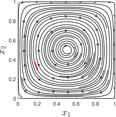
Figure 5: In the first two sub-figures are depicted the vector fields of RD, and the solution of the SIAR problem in (86). The red points indicate the sample data fed in this instance of the SIAR problem. The remaining sub-figures depict the SIAR solution for different subsets of the side-information constraints described in subsection E.1. From left-to-right those subsets are: An empty set of SI constraints, the standalone FI property as given in (84), the standalone PC property as given in (85).

Taking $Q_{0}=Q_{2}=0$ and $Q_{1}=\begin{bmatrix}4&0&-4\\ 0&0&0\\ -4&0&16\end{bmatrix}$ we see that the replicator dynamics (83) are a feasible solution. In Figure 5 we depict the vector field of the RD and the SIAR’s solution along with a number of what-if scenarios where we restrict ourselves to smaller subsets of the side-information constraints. Notice how the SIAR regressor is progressively shaped by the side-information constraints until eventually becomes identical to the RD.

E.2 A Congestion Game with Multiple Equilibria

A congestion game is defined by a graph ${\mathcal{G}}({\mathcal{N}},{\mathcal{E}})$ on $n$ nodes and delay functions ${d}_{e}:\{1,\,\dotsc,\,{n}\}\to\mathbb{R}$, ${e}\in{\mathcal{E}}$, that capture the delay due to congestion conditions in each edge ${e}$ of the graph as a function of the total number of commuters that traverse it. The agents are commuters whose actions are all the possible paths that allow them to travel from some origin node ${{v}_{\mathrm{origin}}}\in{\mathcal{N}}$ to some destination node ${{v}_{\mathrm{destination}}}\in{\mathcal{N}}$.

In this example, we consider a simple instance of a congestion game where each of $n$ agents is presented with two choices of arcs ${\mathcal{A}}=\{e_{1},e_{2}\}$ from a single origin node to a single destination node.

The delay functions ${d}_{{e}_{1}}:\{1,\,\dotsc,\,{n}\}\to\mathbb{R}$, and ${d}_{{e}_{2}}:\{1,\,\dotsc,\,{n}\}\to\mathbb{R}$, are linear, i.e., ${d}_{{e}_{j}}(x)={c}_{{e}_{j}}\cdot x$ where ${c}_{{e}_{j}}>0$. For all action profiles ${a}=(a_{1},\dots,a_{n})\in\{e_{1},e_{2}\}^{n}$, the payoff of each agent ${i}\in{\mathcal{N}}$ in this congestion game is the negative of the total delay along their choice of path, given by:

$$u_{i}(a_{i},a_{-i})=-c_{a_{i}}\cdot|j\in{\mathcal{N}}:a_{j}=a_{i}|,$$ (92)

where $|j\in{\mathcal{N}}:a_{j}=a_{i}|$ is the number of players that choose arc $a_{i}$.

Moreover, in terms of mixed strategies we have that

$$u_{i}({e_{1}},x_{-i}) =-c_{e_{1}}\Big{(}1+\sum_{j\neq i}x_{j}\Big{)}$$ (93)

$$u_{i}({e_{2}},x_{-i}) =-c_{e_{2}}\Big{(}1+\sum_{j\neq i}(1-x_{j})\Big{)}$$

and

$$u_{i}(x_{i},x_{-i})=-x_{i}c_{e_{1}}\Big{(}1+\sum_{j\neq i}x_{j}\Big{)}-(1-x_{i})c_{e_{2}}\Big{(}1+\sum_{j\neq i}(1-x_{j})\Big{)}+c_{e_{2}}\Big{(}1+\sum_{j\neq i}(1-x_{j})\Big{)}$$ (94)

Consequently, using (30) and (93), for the replicator dynamics we have

$$\dot{x}_{i}={{f}^{\mathrm{\acs*{RD}}}_{i}}({x}) ={x}_{i}(1-{x}_{i})(u_{i}(e_{1},x_{-i})-u_{i}(e_{2},x_{-i}))$$ (95a)

$$=x_{i}(1-x_{i})\Big{(}-c_{e_{1}}(1+\sum_{j\neq i}x_{j})+c_{e_{2}}(1+\sum_{j\neq i}(1-x_{j}))\Big{)}$$ (95b)

$$=-{x}_{i}(1-{x}_{i})\Big{(}({c}_{{e}_{1}}+{c}_{{e}_{2}})\sum_{\begin{subarray}{c}{j}=1\\ {j}\neq{i}\end{subarray}}^{{n}}{x}_{j}+{c}_{{e}_{1}}-{c}_{{e}_{2}}\cdot{n}\Big{)},$$ (95c)

where ${x}_{i}\in[0,1]$, ${i}\in{\mathcal{N}}$, denote the probability of each agent ${i}$ of choosing the arc $e_{1}$. Lastly, the positive correlation constraint (37) boils down to:

$$(u_{i}(e^{a_{i1}},x_{-i})-u_{i}(e^{a_{i2}},x_{-i})){{f}^{\mathrm{\acs*{RD}}}_{i}}({x})=-\Big{(}({c}_{{e}_{1}}+{c}_{{e}_{2}})\sum_{\begin{subarray}{c}{j}=1\\ {j}\neq{i}\end{subarray}}^{{n}}{x}_{j}+{c}_{{e}_{1}}-{c}_{{e}_{2}}\cdot{n}\Big{)}{{f}^{\mathrm{\acs*{RD}}}_{i}}({x})\geq 0,$$ (96)

for all $x\in[0,1]^{n}.$ A congestion game, is an anonymous game, as defined in Equation 20 as the delay experienced by an agent depends solely on how many other agents have chosen the same arc, and not on their individual identities. The anonymity of the underlying game allows us to restrict our search space to polynomial regressors that satisfy

$${p}_{i}({x})={p}_{{\pi}({i})}({\pi}^{-1}({x})),\;\text{for all $x\in{\mathcal{X}}$}.$$ (97)

for all ${i}\in{\mathcal{N}}$ and all bijections ${\pi}:{\mathcal{N}}\to{\mathcal{N}}$. Since the state space ${\mathcal{X}}$ is an infinite set, (97), is equivalent to showing that the polynomials ${p}_{i}({x})$ and ${p}_{{\pi}({i})}({\pi}^{-1}({x}))$ are equal for all ${i}\in{\mathcal{N}}$ and for all all bijections ${\pi}:{\mathcal{N}}\to{\mathcal{N}}$. However, the number of such constraints increases exponentially with the number of agents ${n}$. To address this issue, we can observe that (97) implies that given one of the regressors (e.g., ${p}_{1}$ at ${x}$), we can compute all other regressors $p_{i}\geq 2$ at ${x}$. using an appropriate bijection. Thus, our SIAR formulation will only search for a single regressor $p_{1}(x)$. Next, we need to express the loss function

$$\sum_{i=1}^{n}\sum_{k=1}^{K}\Big{(}p_{i}\big{(}x^{(k)}\big{)}-\dot{x}_{i}^{(k)}\Big{)}^{2}$$ (98)

in terms of $p_{1}(x)$ alone. For example, to express the summand $\Big{(}p_{2}\big{(}x^{(k)}_{1},x^{(k)}_{2},x^{(k)}_{-\{1,2\}}\big{)}-\dot{x}_{2}^{(k)}\Big{)}^{2}$ corresponding to the second agent in terms of $p_{1}$, we use (97) where $\pi$ swaps the first two agents, implying that:

$$p_{2}\big{(}x^{(k)}_{1},x^{(k)}_{2},x^{(k)}_{-\{1,2\}}\big{)}=p_{1}\big{(}x^{(k)}_{2},x^{(k)}_{1},x^{(k)}_{-\{1,2\}}\big{)}.$$ (99)

Finally, we need to impose appropriate symmetry constraints on $p_{1}$. These are obtained by (97) for permutations $\pi:{\mathcal{N}}\to{\mathcal{N}}$ that leave agent $1$ invariant, i.e.,

$$p_{1}(x_{1},x_{-1})=p_{1}(x_{1},\pi^{-1}(x_{-1})),\;\text{ where $\pi^{-1}$ is a permutation of $\{2,\,\dotsc,\,n\}$}.$$ (100)

Although, there is still an exponential number of such permutations, these can be enforced by choosing an appropriate monomial basis. For this, note that if we expand $p_{1}$ in terms of powers of $x_{1}$, i.e., $p_{1}(x_{1},x_{-1})=\sum_{j}x_{1}^{j}g^{(j)}(x_{-1})$, (100) implies that

$$\sum_{j}x_{1}^{j}g^{(j)}(x_{-1})=\sum_{j}x_{1}^{j}g^{(j)}(\pi^{-1}(x_{-1})),\;\text{ where $\pi^{-1}$ is a permutation of $\{2,\,\dotsc,\,n\}$},$$ (101)

which in turn implies that each $g^{(j)}$ is a symmetric polynomial. Consequently, each $g^{(j)}$ can be written as a linear combination of the monomial symmetric polynomials [14]. For each vector $b=(b_{2},\dots,b_{n})\in\mathbb{N}^{n}$ the corresponding symmetric monomial $m_{b}(x_{-1})$ is obtained as the sum of all monomials $x_{2}^{c_{2}}\dots x_{n}^{c_{n}}$ where $(c_{2},\dots,c_{n})$ ranges over all distinct permutations of $b$. Putting everything together, the formulation of the SIAR is given as:

$$\underset{p_{1}}{\text{min}} \ \sum_{i=1}^{n}\sum_{k=1}^{K}\Big{(}p_{i}\big{(}x^{(k)}\big{)}-\dot{x}_{i}^{(k)}\Big{)}^{2}$$ (102)

s.t. $$p_{1}(0,x_{-1})\geq 0$$

$$p_{1}(1,x_{-1})\leq 0$$

$$\Big{(}({c}_{{e}_{1}}+{c}_{{e}_{2}})\sum_{\begin{subarray}{c}{j}=1\\ {j}\neq{i}\end{subarray}}^{{n}}{x}_{j}+{c}_{{e}_{1}}-{c}_{{e}_{2}}\cdot{n}\Big{)}\cdot p_{1}(x)\leq 0$$

$$p_{1}(x)=\sum_{c}\sum_{j}\lambda_{jc}x_{1}^{j}m_{c}(x_{-1})$$

Here, the first two constraints express the fact that $p_{1}(x)$ is forward invariant (cf. (34)) and the third constraint expresses that $p_{1}(x)$ satisfies the positive correlation property (cf. (96)). Due to the dimensionality of this example, we can not provide a visualization of the SIAR solution; in contrast, we verify our result using a different approach.

Congestion games like the above are characterized by the existence of an exponential number of equilibrium points, e.g., $\begin{pmatrix}n\\ \frac{n}{2}\end{pmatrix}$ in the aforementioned case, giving rise to an equilibrium selection problem, i.e., how do the agents decide over one equilibrium over the other? RD, i.e., the true dynamical system, as well as LBD, and various other learning dynamics serve as different solutions to the above problem by acting as mechanisms to guide the agents towards one of the multiple equilibrium points of the game [29]. QLD, on the other hand, act as mechanism to differentiate between a similar notion coined Quantal Response Equilibria, which depend on the hyper-parameter $T$ of the dynamics (cf. Appendix B). Nonetheless for small enough values of $T$, the Quantal Response Equilibria of the above game closely match the corresponding Nash equilibria, and therefore, we can test the SIAR framework’s effectiveness under a common, umbrella, methodology. Apparently, due to the above, it is natural to test whether the dynamical system derived by the SIAR solution matches the aforementioned property of the true system, and in other words, solve the agent’s equilibrium selection problem in an identical manner. As it summarized in Table 4 this is indeed the case for solution of the SIAR program in (102). Specifically, when the program is fed with a small data-set, sampled by the true dynamical system, its solution exhibits identical behavior as the RD, or the QLD, respectively. As it turns out, this is true even when the data-set comes from QLD, under a slight modification where the PC property in (102) is replaced with a more general notion (cf. Appendix B).

E.3 A Nickel-Quarter Game

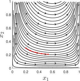
Figure 6: In the first sub-figure is depicted the payoff matrix of the Nickel-Quarter game described in subsection E.3. Th rest of the sub-figures depict the vector fields of the RD in the aforementioned game, and the solution of the SIAR problem as given in (105), respectively. The red points indicate the sample data that was fed in the SIAR regressor during the training.

In the next example, we consider a $2$-agent, $2$-action normal-form game, which, for simplicity, we dub the Nickel-Quarter game. In a Nickel-Quarter game, each agent is given a choice between two coins, a nickel, which worths $5$¢, and a quarter, which worths $25$¢. If at least one of the agents chooses a nickel, then the first player gets both coins and wins the game. Otherwise, the second agent wins and collects the total amount. Note that, in a Nickel-Quarter game, no matter what action the second agent takes, the first agent is better off choosing a nickel than choosing a quarter, and, therefore, for the first agent, the action of choosing a quarter is dominated by the action of choosing a nickel. To break up any ties, in terms of dominance, between the two actions we further assume that the first agent is slightly biased towards choosing a nickel, which we express with some additional reward $\alpha>0$ for choosing this action. The $2\times 2$ payoff matrix that captures the agent payoffs in each of the four outcomes of this game is depicted in Figure 6.

In this example, we assume that the Nickel-Quarter game evolves according to the RD, and, based on the fact the action set of each agent is a binary set, we may, conveniently, capture the game’s evolution in the space ${\mathcal{X}}\equiv[0,1]^{2}$ by the following equations of motion:

$$\dot{x}_{1}={{f}^{\mathrm{\acs*{RD}}}_{1}}({x})\triangleq{x}_{1}(1-{x}_{1})\big{(}50(1-{x}_{2})+\alpha\big{)}$$ (103)

$$\dot{x}_{2}={{f}^{\mathrm{\acs*{RD}}}_{2}}({x})\triangleq 10{x}_{2}(1-{x}_{2})(5{x}_{1}-3),$$

where, ${x}_{1},{x}_{2}\in[0,1]$, denote the chance that the first, and the second agent, respectively, chooses a nickel. However, the observable information we have about the true system is limited. Specifically, we have access to a small number of noisy observations $\{\big{(}{x}({t}_{{k}}),\dot{x}({t}_{{k}})\big{)}\,:\,{{k}}=1,\,\dotsc,\,{K}\}$ of the system, for some ${t}_{1},\,\dotsc,\,{t}_{{K}}\geq 0$, and we are only given the side-information that the agents’ strictly dominated actions are eventually eliminated; which is indeed the case for RD. Formally, our goal is to recover the true equations of motion in (103), and, thus, identifying the true learning dynamics of the game. To do that we are going to construct an appropriate SIAR problem, and approximate its solution using the SOS approach.

Our main challenge in this example is to express the given side-information, namely that the agents’ strictly dominated actions are eventually eliminated, as a set of appropriate polynomial side-information constraints. Towards overcoming the above challenge we are going to construct a set of side-information constraints that ensure the sufficient condition that the estimated dynamics are RSD, and satisfy the CM property. Let ${p}_{1}$, and ${p}_{2}$ be some estimates of ${{f}^{\mathrm{\acs*{RD}}}_{1}}$, and ${{f}^{\mathrm{\acs*{RD}}}_{2}}$ in (103), respectively. As a first step, we need to state the side-information constraints that restrict the dynamics of the recovered system, given by $\dot{x}_{i}={p}_{i}({x})$, ${i}\in\{1,2\}$, to be RSD. Simply enough, following the definition of RSD, we need to find some functions $\tilde{{p}}_{{i}{{a}_{{i}}}}$, ${i}\in\{1,2\}$, ${{a}_{{i}}}\in\{{\mathrm{Nickel}},{\mathrm{Quarter}}\}$, Lipschitz continuous in ${\mathcal{X}}$, such that ${p}_{i}({x})={x}_{i}\tilde{{p}}_{{i},{\mathrm{Nickel}}}({x})=-(1-{x}_{i})\tilde{{p}}_{{i},{\mathrm{Quarter}}}({x})$, for all states ${x}\in{\mathcal{X}}$, and for all agents ${i}\in\{1,2\}$, Note that, if we restrict our search to $\tilde{{p}}_{{i}{{a}_{{i}}}}$, ${i}\in\{1,2\}$, ${{a}_{{i}}}\in\{{\mathrm{Nickel}},{\mathrm{Quarter}}\}$, that are polynomial, and, since ${p}_{i}$ is also a polynomial, and ${\mathcal{X}}$ is infinite, we may incorporate the first condition by imposing the equality constraints ${p}_{i}({x})={x}_{i}\tilde{{p}}_{{i},{\mathrm{Nickel}}}({x})=-(1-{x}_{i})\tilde{{p}}_{{i},{\mathrm{Quarter}}}({x})$, for all ${x}\in\mathbb{R}^{2}$, in the SIAR problem’s formulation. Notice that, in this case, we do not need restrict ${x}\in{\mathcal{X}}$, and since ${\mathcal{X}}$ is compact, any polynomial $\tilde{{p}}_{{i}{{a}_{{i}}}}$, ${i}\in\{1,2\}$, ${{a}_{{i}}}\in\{{\mathrm{Nickel}},{\mathrm{Quarter}}\}$, we find is bound to be Lipschitz continuous.

Next, in order to impose that estimated system satisfies the CM property, we have to begin by characterizing all the strictly dominated actions in the Nickel-Quarter game, as well as, the set of states over the action space ${\mathcal{X}}$ that dominate each one. It is trivial to see that no action of the second agent strictly dominates the other. On the other hand, since by choosing a nickel the first agent is always striclty better off than choosing a quarter, and since choosing a quarter it’s, trivially, a dominant action to itself, we have, by convexity, that ${u}_{1}(0,{x}_{2})\leq{u}_{1}({x})$, for all ${x}\in{\mathcal{X}}$. Then, from the CM property’s definition (cf. 3), we get the constraint that, for all $\tilde{{x}}_{1}\in(0,1]$, and for all ${x}\in{\mathcal{X}}$:

$$0 <\tilde{{x}}_{1}\tilde{{p}}_{1,{\mathrm{Nickel}}}({x})+(1-\tilde{{x}}_{1})\tilde{{p}}_{1,{\mathrm{Quarter}}}({x})-\tilde{{p}}_{1,{\mathrm{Quarter}}}({x})$$ (104a)

$$=\tilde{{x}}_{1}\big{(}\tilde{{p}}_{1,{\mathrm{Nickel}}}({x})-\tilde{{p}}_{1,{\mathrm{Quarter}}}({x})\big{)}$$ (104b)

Furthermore, since (104a) holds for all $\tilde{{x}}_{1}\in(0,1]$, the above is equivalent to $\tilde{{p}}_{1,{\mathrm{Nickel}}}-\tilde{{p}}_{1,{\mathrm{Quarter}}}>0$ for all ${x}\in{\mathcal{X}}$. In other words, in order for the estimated system to satisfy the CM property we simply need to restrict our search for $\tilde{{p}}_{1,{{a}_{{i}}}}$, ${{a}_{{i}}}\in\{{\mathrm{Nickel}},{\mathrm{Quarter}}\}$, such that $\tilde{{p}}_{1,{\mathrm{Nickel}}}({x})-\tilde{{p}}_{1,{\mathrm{Quarter}}}({x})\geq\epsilon$, for all ${x}\in{\mathcal{X}}$, for some small $\epsilon>0$, that

Putting everything together, we come up with the following formulation of a SIAR problem:

$$\underset{{p},\tilde{{p}}}{\text{minimize}} \sum_{{i}=1}^{2}\sum_{{{k}}=1}^{{K}}\big{[}{p}_{i}\big{(}{x}({t}_{{k}})\big{)}-\dot{x}_{i}({t}_{{k}})\big{]}^{2}$$ (105)

subject to $${p}_{i}({x})={x}_{i}\tilde{{p}}_{{i},{\mathrm{Nickel}}}({x}),\;\text{for all ${x}\in\mathbb{R}^{2}$}$$

$${p}_{i}({x})=-(1-{x}_{i})\tilde{{p}}_{{i},{\mathrm{Quarter}}}({x}),\;\text{for all ${x}\in\mathbb{R}^{2}$}$$

$$\tilde{{p}}_{1,{\mathrm{Nickel}}}({x})-\tilde{{p}}_{1,{\mathrm{Quarter}}}({x})\geq\epsilon,\;\text{for all ${x}\in{\mathcal{X}}$}.$$

As in the previous example, we may approximate a solution to the above SIAR problem using a hierarchy of SOS relaxations, where we strengthen the non-negativity constraint $\tilde{{p}}_{1,{\mathrm{Nickel}}}({x})-\tilde{{p}}_{1,{\mathrm{Quarter}}}({x})\geq\epsilon$ to $\tilde{{p}}_{1,{\mathrm{Nickel}}}({x})-\tilde{{p}}_{1,{\mathrm{Quarter}}}({x})-\epsilon\in\mathrm{SOS}$. In Figure 6 we depict the vector field of the SIAR solution compared to the one of the RD. Note that the side-information properties used in this case are substantially weaker than in the previous examples.

E.4 A Chaotic *RPS Game

As a last application, we consider an instance of an $\epsilon$-perturbed RPS game. A standard RPS game is characterized as a zero-sum normal-form game between two players, where each player is given three possible actions, namely, Rock, Paper, or Scissors. No single action is preferable over the rest, with Rock ruling over Scissors, Scissors ruling over Paper, and Paper ruling over Rock. In a standard RPS draws, i.e.,, a game outcome where both player have chosen the same action, do not favor a particular player. In an $\epsilon$-perturbed RPS game though, the symmetry of the game breaks down by deciding to resolve draws slightly in favor of one of the two players. Algebraically, the utility functions of a $\epsilon$-perturbed RPS are given by:

$$u_{1}(x_{1},x_{2})=-u_{2}(x_{1},x_{2})=x_{1}^{\intercal}(A+\epsilon\cdot{\mathbf{I}})x_{2},\;\text{for all $x\in{\mathcal{X}}$}\;\text{with $A=\begin{bmatrix}[r]0&-1&1\\ 1&0&-1\\ -1&1&0\end{bmatrix}$, and $-1<\epsilon<1$}.$$ (106)

In this example, we are going to assume that an $\epsilon$-perturbed RPS game evolves according to the RD given by:

$$\dot{x}_{ia_{i}}={{f}^{\mathrm{\acs*{RD}}}_{ia_{i}}}(x)\triangleq x_{ia_{i}}\big{(}u_{i}(e^{a_{i}},x_{2})-u_{i}(x)\big{)}\;\text{for all $x\in{\mathcal{X}}$, $i=1,2$, and $a_{i}\in\{\mathrm{Rock(R)},\mathrm{Paper(P)},\mathrm{Scissors(S)}\}$}.$$ (107)

As before, the observable information we have about the system is limited. Specifically, we have access to a small number of noisy observations $\big{\{}\big{(}{x}({t}_{{k}}),\dot{x}({t}_{{k}})\big{)}\,:\,{{k}}=1,\,\dotsc,\,{K}\big{\}}$, for some ${t}_{1},\,\dotsc,\,{t}_{{K}}\geq 0$, and we are given the side-information that the the state space ${\mathcal{X}}$ is forward-invariant, and the PC property is satisfied by the original system. Formally, in an ideal setup, our goal is to recover the true equations of motion in (107), and, thus, identifying the true learning dynamics of the game. To do that we are going to construct an appropriate SIAR problem, and approximate its solution using the SOS approach.

A factor that sets this particular setup apart from the previous exhibitions is the behavior of RD in a game of $\epsilon$-RPS. While in a standard RPS, i.e.,, $\epsilon=0$, RD are known to converge to a limit cycle, in a $\epsilon$-perturbed RPS, they exhibit chaotic behavior, which becomes more apparent as $\epsilon$ moves away from zero [30]. Informally a dynamical system exhibits chaotic behavior if small perturbations in the system’s initialization lead to radically different trajectories. One possible way to visualize the chaotic aspect of the evolution RD in the above setup is through a Poincaré section; a technique that depicts other additional qualitative factors of the evolution as well. A Poincaré section depicts the points that a trajectory, or a set of trajectories, of the system crosses a lower-dimensional subspace of the state space ${\mathcal{X}}$. As an example, in Figure 7, we depict the Poincaré section $\{x\in{\mathcal{X}}\,:\,x_{i,\mathrm{Rock}}-x_{i,\mathrm{Paper}}=0\}$ for a set of trajectories initialized at $x_{1}(0)=(0.5,0.025\cdot m,0.5-0.025\cdot m)$, where $m=1,\,\dotsc,\,10$, and $x_{2}(0)=(0.5,0.25,0.25)$ for $\epsilon=0.25$. Observe that the pattern signifying the recurrent behavior of the RD in a standard RPS, gradually in trajectories initialized closer to the boundary of the state space.

Moving back to our initial ideal goal of perfectly recovering the true equation of motion of the above system, i.e.,, the RD, it is apparent, due to the finite precision of any numerical method, that perfect recovery cannot be achieved in case that $\epsilon\neq 0$. Therefore, we relax our initial expectations and settle with identifying a system that closely approximates the ground truth learning dynamics for as long as possible, given the limited information we have at hand. To evaluate the SIAR problem’s solution, both visually, and numerically, we are going to rely on two quantifiers: a Poincaré section, explained above, and the maximum Lyapunov exponent. The maximum Lyapunov exponent of the system is a quantifier of how radically the behavior of the chaotic system changes for negligible perturbations $\delta>0$ of its initial conditions, given by the formula:

$$\lambda_{\max}=\max_{\begin{subarray}{c}i=1,2\\ a_{i}\in\{\mathrm{R},\mathrm{P},\mathrm{S}\}\end{subarray}}\lim_{t\to\infty}\lim_{\delta\to 0}\frac{1}{t}\ln\frac{\lvert x_{ia_{i}}(t)-x^{\prime}_{ia_{i}}(t)\rvert}{\delta},$$ (108)

A positive maximum Lyapunov exponent $\lambda_{\max}$ is an indication of chaotic behavior, with larger magnitudes corresponding to more unpredictable trajectory evolution.

We treat the problem similarly to the previous examples, namely, we let ${p}_{ia_{i}}$ be some estimate of ${{f}^{\mathrm{\acs*{RD}}}_{ia_{i}}}$, for $i=1,2$, and $a_{i}\in\{\mathrm{R},\mathrm{P},\mathrm{S}\}$, and we begin by constructing the side-information constraints that we are going to impose to the SIAR problem. In this case, the imposing constraints follow directly from the definitions of the forward invariance of the state space ${\mathcal{X}}$, and the PC property of the system. The complete formulation of the SIAR problem is given as:

$$\underset{{p}}{\text{minimize}} \sum_{{i}=1}^{2}\sum_{{{k}}=1}^{{K}}\big{\lVert}{p}_{i}\big{(}{x}({t}_{{k}})\big{)}-\dot{x}_{i}({t}_{{k}})\big{\rVert}^{2}$$ (109)

subject to $$\sum_{a_{i}\in\{\mathrm{R},\mathrm{P},\mathrm{S}\}}{p}_{ia_{i}}({x})=0,\;\text{for all ${x}\in\mathbb{R}^{3}\times\mathbb{R}^{3}$}$$

$${p}_{ia_{i}}({x})\geq 0,\;\text{for all ${x}\in{\mathcal{X}}$ whenever $x_{ia_{i}}=0$}$$

$$\sum_{a_{i}\in\{\mathrm{R},\mathrm{P},\mathrm{S}\}}{u}_{ia_{i}}(x){p}_{ia_{i}}(x)\geq 0,\;\text{for all ${x}\in{\mathcal{X}}$}.$$

In Figure 7 we compare the SIAR solution to the behavior of the true dynamical system using as reference the same Poincaré section. Notice that the behavior of the SIAR solution not only closely matches the one of the RD in the more predictable trajectories, i.e., the ones initialized further from the boundary of the state space, but also the system’s trajectories become more scrabbled for initializations closer to the boundary, in a similar manner as the ones of the true system. In Figure 8 we numerically quantify the error between each of those trajectories with time measures in Lyapunov times. As it turns out the SIAR solution provides such an accurate estimate that closely reassembles the system even up to $8$ Lyapunov times.

Table 4: Accuracy(%) of the SIAR solution in the problem of predicting the equilibrium points of convergence of RD, LBD, and QLD in the congestion game described in subsection E.2. The parameters, $n$, and $d$, refer to the number of agents, and the degree of the SIAR’s solution. Despite the difficulty of the Equilibrium Selection problem in this game’s instance, the SIAR solution exhibits remarkable accuracy, even in cases where the underlying dynamics are non-polynomials, e.g.,, QLD.

	*RD		*LBD		*QLD
$n$	$d=4$	$d=5$	$d=4$	$d=5$	$d=4$	$d=5$
$2$	$100$	$99.99$	$99.99$	$99.99$	$96.12$	$99.99$
$4$	$100$	$100$	$100$	$100$	$99.82$	$100$
$6$	$100$	$100$	$100$	$100$	$100$	$100$
$8$	$100$	$100$	$100$	$100$	$100$	$100$
$10$	$100$	$100$	$99.98$	$99.97$	$100$	$100$

Figure 7: The Poincaré section $\{x\in{\mathcal{X}}\,:\,x_{i,\mathrm{Rock}}-x_{i,\mathrm{Paper}}=0\}$ for a set of trajectories initialized at $x_{1}(0)=(0.5,0.025\cdot m,0.5-0.025\cdot m)$, where $m=1,\,\dotsc,\,10$, and $x_{2}(0)=(0.5,0.25,0.25)$ for the RD (left), and the solution of the SIAR problem given in (109) (right) for the $0.25$-perturbed RPS game described in subsection E.4.

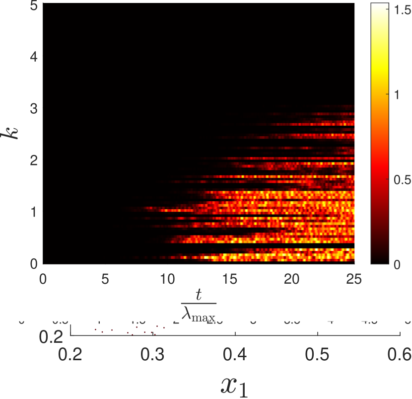
Figure 8: The error of the SIAR problem’s solution for the for a set of trajectories initialized at $x_{1}(0)=(0.5,0.025\cdot m,0.5-0.025\cdot k)$, where $k=1,\,\dotsc,\,10$, and $x_{2}(0)=(0.5,0.25,0.25)$ compared the corresponding trajectories of RD in the $0.25$-perturbed RPS game. The time is measured in Lyapunov times $t/\lambda_{\max}$ in to depict the robusticity of the SIAR solution in a chaotic environment.

References

- Silver et al. [2016] David Silver, Aja Huang, Chris J. Maddison, Arthur Guez, Laurent Sifre, George van den Driessche, Julian Schrittwieser, Ioannis Antonoglou, Veda Panneershelvam, Marc Lanctot, Sander Dieleman, Dominik Grewe, John Nham, Nal Kalchbrenner, Ilya Sutskever, Timothy Lillicrap, Madeleine Leach, Koray Kavukcuoglu, Thore Graepel, and Demis Hassabis. Mastering the game of go with deep neural networks and tree search. Nature, 529(7587):484–489, Jan 2016. ISSN 1476-4687. doi: 10.1038/nature16961.
- Schmid et al. [2021] Martin Schmid, Matej Moravcik, Neil Burch, Rudolf Kadlec, Josh Davidson, Kevin Waugh, Nolan Bard, Finbarr Timbers, Marc Lanctot, Zach Holland, Elnaz Davoodi, Alden Christianson, and Michael Bowling. Player of games, 2021.
- Haarnoja et al. [2023] Tuomas Haarnoja, Ben Moran, Guy Lever, Sandy H. Huang, Dhruva Tirumala, Markus Wulfmeier, Jan Humplik, Saran Tunyasuvunakool, Noah Y. Siegel, Roland Hafner, Michael Bloesch, Kristian Hartikainen, Arunkumar Byravan, Leonard Hasenclever, Yuval Tassa, Fereshteh Sadeghi, Nathan Batchelor, Federico Casarini, Stefano Saliceti, Charles Game, Neil Sreendra, Kushal Patel, Marlon Gwira, Andrea Huber, Nicole Hurley, Francesco Nori, Raia Hadsell, and Nicolas Heess. Learning agile soccer skills for a bipedal robot with deep reinforcement learning, 2023.
- Bard et al. [2019] Nolan Bard, Jakob N. Foerster, Sarath Chandar, Neil Burch, Marc Lanctot, H. Francis Song, Emilio Parisotto, Vincent Dumoulin, Subhodeep Moitra, Edward Hughes, Iain Dunning, Shibl Mourad, Hugo Larochelle, Marc G. Bellemare, and Michael Bowling. The hanabi challenge: A new frontier for ai research, 2019.
- Brunton and Kutz [2019] Steven L. Brunton and J. Nathan Kutz. Data-driven science and engineering. Cambridge University Press, Cambridge, England, February 2019. ISBN 978-1-10842-209-3.
- Icke and Bongard [2013] Ilknur Icke and Joshua C. Bongard. Modeling hierarchy using symbolic regression. In 2013 IEEE Congress on Evolutionary Computation, pages 2980–2987, 2013. doi: 10.1109/CEC.2013.6557932.
- Brunton et al. [2016] Steven L. Brunton, Joshua L. Proctor, and J. Nathan Kutz. Discovering governing equations from data by sparse identification of nonlinear dynamical systems. Proceedings of the National Academy of Sciences, 113(15):3932–3937, 2016. doi: 10.1073/pnas.1517384113.
- Rudy et al. [2017] Samuel H. Rudy, Steven L. Brunton, Joshua L. Proctor, and J. Nathan Kutz. Data-driven discovery of partial differential equations. Science Advances, 3, 2017. doi: 10.1126/sciadv.1602614.
- Kaiser et al. [2018] E. Kaiser, J. Nathan Kutz, and Steven L. Brunton. Sparse identification of nonlinear dynamics for model predictive control in the low-data limit. Proceedings of the Royal Society A: Mathematical, Physical and Engineering Sciences, 474, 2018. doi: 10.1098/rspa.2018.0335.
- Curmei and Hall [2022] Mihaela Curmei and Georgina Hall. Shape-constrained regression using sum of squares polynomials, 2022.
- Ahmadi and Khadir [2023] Amir Ali Ahmadi and Bachir El Khadir. Learning dynamical systems with side information. SIAM Review, 65(1):183–223, 2023. doi: 10.1137/20M1388644.
- Swinkels [1993] Jeroen M. Swinkels. Adjustment dynamics and rational play in games. Games and Economic Behavior, 5:455–484, 1993. ISSN 0899-8256. doi: 10.1006/game.1993.1025.
- Sandholm [2010] William H. Sandholm. Population games and evolutionary dynamics. Economic Learning and Social Evolution. MIT Press, London, England, December 2010. ISBN 978-0-2621-9587-4.
- Brandt et al. [2009] Felix Brandt, Felix Fischer, and Markus Holzer. Symmetries and the complexity of pure nash equilibrium. Journal of Computer and System Sciences, 75(3):163–177, 2009. ISSN 0022-0000. doi: 10.1016/j.jcss.2008.09.001.
- Nash [1951] John Nash. Non-cooperative games. Annals of Mathematics, 54:286–295, 1951. ISSN 0003-486X. doi: 10.2307/1969529.
- Daskalakis et al. [2009] Constantinos Daskalakis, Paul W. Goldberg, and Christos H. Papadimitriou. The complexity of computing a nash equilibrium. Commun. ACM, 52(2):89–97, feb 2009. ISSN 0001-0782. doi: 10.1145/1461928.1461951.
- Parrilo and Thomas [2020] Pablo A. Parrilo and Rekha R. Thomas. Positive Polynomials: From Hilbert’s 17th Problem to Real Algebra. Springer Berlin, Heidelberg, 2020. ISBN 978-3-540-41215-1. doi: 10.1007/978-3-662-04648-7.
- Lasserre [2007] Jean B. Lasserre. A sum of squares approximation of nonnegative polynomials. SIAM Review, 49(4):651–669, 2007. ISSN 0036-1445. doi: 10.1137/070693709.
- Parrilo [2000] Pablo A Parrilo. Structured semidefinite programs and semialgebraic geometry methods in robustness and optimization. PhD thesis, California Institute of Technology, 2000.
- Parrilo [2003] Pablo A. Parrilo. Semidefinite programming relaxations for semialgebraic problems. Mathematical Programming, 96(2):293–320, May 2003. ISSN 1436-4646. doi: 10.1007/s10107-003-0387-5.
- Lasserre [2001] Jean B. Lasserre. Global optimization with polynomials and the problem of moments. SIAM Journal on Optimization, 11(3):796–817, 2001. doi: 10.1137/S1052623400366802.
- Laurent [2009] Monique Laurent. Sums of Squares, Moment Matrices and Optimization Over Polynomials, pages 157–270. Springer New York, New York, NY, 2009. ISBN 978-0-387-09686-5. doi: 10.1007/978-0-387-09686-5_7.
- Nagumo [1942] Mitio Nagumo. Über die lage der integralkurven gewöhnlicher differentialgleichungen. In Proceedings of the Physico-Mathematical Society of Japan, 1942. doi: 10.11429/PPMSJ1919.24.0_551.
- Schuster and Sigmund [1983] Peter Schuster and Karl Sigmund. Replicator dynamics. Journal of Theoretical Biology, 100:533–538, 1983. ISSN 0022-5193. doi: 10.1016/0022-5193(83)90445-9.
- Taylor and Jonker [1978] Peter D. Taylor and Leo B. Jonker. Evolutionary stable strategies and game dynamics. Mathematical Biosciences, 40(1):145–156, 1978. ISSN 0025-5564. doi: 10.1016/0025-5564(78)90077-9.
- Bayer and Lagarias [1989] D. A. Bayer and J. C. Lagarias. The nonlinear geometry of linear programming. i affine and projective scaling trajectories. Transactions of the American Mathematical Society, 314(2):499–526, 1989. ISSN 0002-9947. doi: 10.2307/2001396.
- Tuyls et al. [2003] Karl Tuyls, Katja Verbeeck, and Tom Lenaerts. A selection-mutation model for q-learning in multi-agent systems. In Proceedings of the Second International Joint Conference on Autonomous Agents and Multiagent Systems, AAMAS ’03, pages 693––700, New York, NY, USA, 2003. Association for Computing Machinery. ISBN 1581136838. doi: 10.1145/860575.860687.
- ApS [2019] MOSEK ApS. MOSEK Optimizer API for C 10.0.46., 2019. URL https://docs.mosek.com/latest/capi/index.html.
- Kleinberg et al. [2009] Robert Kleinberg, Georgios Piliouras, and Eva Tardos. Multiplicative updates outperform generic no-regret learning in congestion games: Extended abstract. In Proceedings of the Forty-First Annual ACM Symposium on Theory of Computing, STOC ’09, pages 533–542, New York, NY, USA, 2009. Association for Computing Machinery. ISBN 9781605585062. doi: 10.1145/1536414.1536487.
- Sato et al. [2002] Yuzuru Sato, Eizo Akiyama, and J Doyne Farmer. Chaos in learning a simple two-person game. Proceedings of the National Academy of Sciences, 99(7):4748–4751, 2002. doi: 10.1073/pnas.032086299.
- Hofbauer and Weibull [1996] Josef Hofbauer and Jörgen W. Weibull. Evolutionary selection against dominated strategies. Journal of Economic Theory, 71(2):558–573, 1996. ISSN 0022-0531. doi: 10.1006/jeth.1996.0133.
- Alexander and Charles [2011] Prestel Alexander and Delzell Charles. Sum of Squares: Theory and Applications. Springer Berlin Heidelberg, 2011. ISBN 978-1-4704-5025-0.
Appendix A \acl*SIAR: Overview