Abstract

This paper deals with the trade-off between time, workload, and versatility in self-stabilization, a general and lightweight fault-tolerant concept in distributed computing.

In this context, we propose a transformer that provides an asynchronous silent self-stabilizing version $Trans({AlgI})$ of any terminating synchronous algorithm ${AlgI}$. The transformed algorithm $Trans({AlgI})$ works under the distributed unfair daemon and is efficient both in moves and rounds.

Our transformer allows to easily obtain fully-polynomial silent self-stabilizing solutions that are also asymptotically optimal in rounds.

We illustrate the efficiency and versatility of our transformer with several efficient (i.e., fully-polynomial) silent self-stabilizing instances solving major distributed computing problems, namely vertex coloring, Breadth-First Search (BFS) spanning tree construction, $k$-clustering, and leader election.

1 Introduction

Fault tolerance is a main concern in distributed computing, but is often hard to achieve; see, e.g., [31]. Furthermore, when it can be achieved, it often comes at the the price of sacrificing efficiency (in time, space, or workload) or versatility; see, e.g., [16, 12]. In this paper, we tackle the trade-off between time, workload, and versatility in self-stabilization [25], a general and lightweight fault-tolerant concept in distributed computing [4]. Precisely, we consider a specialization of self-stabilization called silent self-stabilization [28].

Starting from an arbitrary configuration, a self-stabilizing algorithm enables the system to recover within finite time a so-called legitimate configuration from which it satisfies an intended specification. Regardless its initial configuration, a silent self-stabilizing algorithm [28] reaches within finite time a configuration from which the values of the communication registers used by the algorithm remain fixed. Notice that silent self-stabilization is particularly suited for solving static problems such as leader election, coloring, or spanning tree constructions. Moreover, as noted in [28], silence is a desirable property. For example, it usually implies more simplicity in the algorithmic design since silent algorithms can be easily composed with other algorithms to solve more complex tasks [4].

Since the arbitrary initial configuration of a self-stabilizing system can be seen as the result of a finite number of transient faults, self-stabilization is commonly considered as a general approach for tolerating such faults in a distributed system [27, 4]. Indeed, self-stabilization makes no hypotheses on the nature (e.g., memory corruption or topological changes) or extent of transient faults that could hit the system, and a self-stabilizing system recovers from the effects of those faults in a unified manner.

However, such versatility comes at a price, e.g., after transient faults cease, there is a finite period of time, called the stabilization phase, during which the safety properties of the system are violated. Hence, self-stabilizing algorithms are mainly compared according to their stabilization time, the worst-case duration of the stabilization phase.

In the distributed computing community, the correctness and efficiency of algorithms is usually established by paper-and-pencil proofs. Such proofs require the formal definition of a computational model for which the distributed algorithm is dedicated. The atomic-state model [25] is the most commonly used model in the self-stabilizing area. This model is actually a shared memory model with composite atomicity: the state of each node is stored into registers and these registers can be directly read by neighboring nodes; moreover, in one atomic step, a node can read its state and that of its neighbors, perform some local computations, and update its state. Hence, executions in this model proceed in atomic steps in which some enabled nodes move, i.e., modify their local state. The asynchrony of the system is materialized by the notion of daemon that restricts the set of possible executions. The weakest (i.e., the most general) daemon is the distributed unfair daemon. Hence, solutions stabilizing under such an assumption are highly desirable, because they work under any daemon assumption.

The stabilization time of self-stabilizing algorithms is usually evaluated in terms of rounds, which capture the execution time according to the speed of the slowest nodes. However, another crucial issue is the number of local state updates, i.e., the number of moves. By definition, the stabilization time in moves captures the total amount of computations an algorithm needs in order to recover a correct behavior. Hence, the move complexity is rather a measure of work than a measure of time. Now, minimizing the number of state modifications allows the algorithm to use less communication operations and communication bandwidth. As explained in [28, 4], to implement an atomic-state model solution in message passing, all nodes should permanently check whether or not they should change their local state due to the modification of some neighbors’ local states. Now, instead of regularly sending maybe heavy messages containing the full node local state, one can adopt the lightweight approach proposed in [28]: nodes regularly send a proof that the value of their state has not changed; then, a node requests the full local state of a neighbor only after a received proof shows a state modification. Such proof can be very small compared to the real local state: the node can just randomly generate a nonce, salt the hash of its local state with this nonce, and finally send a “small” message containing the hash value together with the nonce. In this way, the number of “heavy” messages (i.e., those containing the current local state of some node) depends on the number of moves, and the minimization of the number of moves permits to drastically reduced the communication bandwidth usage. This is especially true when the self-stabilizing solution is silent [28], as in this case there is no more moves after the legitimacy is reached, and from that point, only small proofs are regularly sent.

Until now, in the atomic-state model, techniques to design an algorithm achieving a stabilization time polynomial in moves usually made its rounds complexity inherently linear in $n$, the number of nodes; see, e.g., [14, 3, 23]. Now, the classical nontrivial lower bounds for many problems is $\Omega(D)$ rounds [32], where $D$ is the network diameter. Moreover, in many large-scale networks, the diameter is rather logarithmic on $n$, so finding solutions achieving round complexities linear in $D$ is more desirable. Yet, only a few asynchronous solutions (still in the atomic-state model) achieving such an upper bound exist, e.g., the atomic-state version of the Dolev’s BFS algorithm [26] given in [24]. Moreover, it has been shown that several of them actually have a worst-case execution that is exponential in moves; see [24]. So, it seems that efficiency in rounds and moves are often incompatible goals. In a best-effort spirit, Cournier et al. [15] have proposed to study what they call fully-polynomial stabilizing solutions, i.e., stabilizing algorithms whose round complexity is polynomial on the network diameter and move complexity is polynomial on the network size. As an illustrative example, they have proposed a silent self-stabilizing BFS spanning tree algorithm that stabilizes in $O(n^{6})$ moves and $O(D^{2})$ rounds in a rooted connected network. Until now, it was the only asynchronous self-stabilizing algorithm of the literature achieving this property.

1.1 Contribution

In this paper, we address the issue of generalizing the fully-polynomial approach in the atomic-state model to obtain silent self-stabilizing solutions that are efficient both in rounds and moves.

To that goal, we propose to exploit the links, highlighted in [40], between the Local model [41] and self-stabilization in order to design an efficient transformer, i.e., a meta-algorithm that transforms an input algorithm that does not achieve a desired property (here, self-stabilization) into an algorithm achieving that property.

Our transformer provides an asynchronous silent self-stabilizing version $Trans({AlgI})$ of any terminating synchronous algorithm ${AlgI}$ which works under the distributed unfair daemon and is efficient both in moves and rounds. Precisely, our transformer has several inputs: the algorithm ${AlgI}$ to transform, a flag $f$ indicating the used transformation mode, and optionally a bound ${B}$ on the execution time of ${AlgI}$.

We have two modes for the transformation depending on whether the transformation is lazy or greedy. In both modes, the number of moves of $Trans({AlgI})$ to reach a terminal configuration is polynomial, in $n$ and the synchronous execution time ${T}$ of ${AlgI}$ in the lazy mode, in $n$ and ${B}$ otherwise. An overview of $Trans({AlgI})$ properties (memory requirement, convergence in rounds, convergence in moves) according to the both parameters is presented in Table 1.

In the lazy mode, the output algorithm $Trans({AlgI})$ stabilizes in $O(D+{T})$ rounds where ${T}$ is the actual execution time of ${AlgI}$. Moreover, if the upper bound ${B}$ is given, then the memory requirement of $Trans({AlgI})$ is bounded (precisely, we obtain a memory requirement in $O({B}\times M)$ bits per node, where $M$ is the memory requirement of ${AlgI}$) .

In the greedy mode, $Trans({AlgI})$ stabilizes in $O({B})$ rounds and its memory requirement is also bounded (still $O({B}\times M)$ bits per node).

Our transformer allows to drastically simplify the design of self-stabilizing solutions since it reduces the initial problem to the implementation of an algorithm just working in synchronous settings with a pre-defined initial configuration. Moreover, this simplicity does not come at the price of sacrificing efficiency since it allows to easily implement fully-polynomial solutions.

Finally, our method is versatile, because compatible with most of distributed computing models. Indeed, except when the computation of a state of the input algorithm requires it, our transformer does not use node identifiers nor local port numbers. More precisely, each move is made based on the state of the node and the set of the neighbors’ states (if several neighbors have the same state $s$, the number of occurrences of $s$ is not used to manage the simulation). Therefore, our transformer can be used in strong models with node identifiers like the Local model [41], down to models almost as weak as the stone age model [30].

Our solution is very efficient in terms of time and workload, but at the price of multiplying the memory cost of the original algorithm by its execution time. This time (and thus the multiplicative factor) is however usually small in powerful models such as the Local model. As an illustrative example, this multiplicative memory overhead can be as low as $O(\log^{*}n)$ for very fast algorithms such as the Cole and Vishkin’s coloring algorithm [13]. Furthermore, using nonces and hashes similarly as explained before, one can reduce the communication cost to almost the one of the original algorithm. Indeed, our transformer always modifies its state in a way which can be described with limited information, linear in the time and memory complexity of the simulated algorithm.

We illustrate the efficiency and versatility of our proposal with several efficient (i.e., fully-polynomial) silent self-stabilizing solutions for major distributed computing problems, namely vertex coloring, Breadth-First Search (BFS) spanning tree construction, $k$-clustering, and leader election. In particular, we positively answer to some open questions raised in the conclusion of [15]: (1) there exists a fully-polynomial (silent) self-stabilizing solution for the BFS spanning tree construction whose stabilization time in rounds is asymptotically linear in $D$ (and so asymptotically optimal in rounds), and (2) there exists a fully-polynomial (silent) self-stabilizing solution for the leader election (also with a stabilization time in rounds that is linear in $D$ and so asymptotically optimal in terms of rounds). Finally, we can also design for the first time (to the best of our knowledge) asynchronous fully-polynomial self-stabilizing algorithms with a stabilization time in rounds that can be sublinear in $D$, as shown with our vertex coloring instance that can stabilize in $O(\log^{*}n)$ rounds in unidirectional rings using the right parameters.

	Move complexity	Round complexity
Lazy mode	$O(\min(n^{3}+nT,n^{2}{B}))$	$O(D+T)$
Greedy mode	$O(\min(n^{3}+n{B},n^{2}{B}))$	$O(B)$
Common features
Error recovery	$O(\min(n^{3},n^{2}{B}))$	$O(\min(D,B))$
Space complexity	${B}\cdot M$

• $T$ and $M$ are respectively the time and space complexities of ${AlgI}$.

• $B$ is a parameter $\in\mathbb{N}\cup\{+\infty\}$.

• The algorithm is always silent when ${B}<+\infty$. Here, we assume that $T\leq{B}$.

Table 1: Overview of the properties of $Trans({AlgI})$.

1.2 Related Work

Proposing transformers (also called compilers) is a very popular generic approach in self-stabilization. Transformers are useful to establish expressiveness of a given property: by giving a general construction, they allow to exhibit a class of problems that can achieve a given property. An impossibility proof should be then proposed to show that the property is not achievable out of the class, giving thus a full characterization. For example, Katz and Perry [38] have addressed the expressiveness of self-stabilization in message-passing systems where links are reliable and have unbounded capacity, and nodes are both identified and equipped of infinite local memories. Several transformers, e.g., [11, 38], builds time-efficient self-stabilizing solutions yet working synchronous systems only. Bold and Vigna [11] proposes a universal transformer for synchronous networks. As in [38], the transformer allows to self-stabilize any behavior for which there exists a self-stabilizing solution. The produced output algorithm stabilizes in at most $n+D$ rounds. However, the transformer is costly in terms of local memories (basically, each node collects and stores information about the whole network). In the same vein, Afek and Dolev [1] propose to collect pyramids of views of the system to detect incoherences and correct the behavior of a synchronous system. In [10], Blin et al. propose two transformers in the atomic-state model to construct silent self-stabilizing algorithms. The first one aims at optimizing space complexity: if a task has a proof-labeling scheme that uses $\ell$ bits, then the output algorithm computes the task in a silent and self-stabilizing manner using $O(\ell+\log n)$ bits per node. However, for some instances, it requires an exponential number of rounds. The second one guarantees a stabilization time in $O(n)$ rounds using $O(n^{2}+k\cdot n)$ bits per node for every task that uses a $k$-bit output at each node. Transformers have been also used to compare expressiveness of computational models. Equivalence (in terms of computational power) between the atomic-state model and the register one and between the register model and message passing are discussed in [27]. In [43], Turau proposes a general transformation procedure that allows to emulate any algorithm for the distance-two atomic-state model in the (classical) distance-one atomic-state model assuming that nodes have unique identifiers.

It is important to note that the versatility is often obtained at the price of inefficiency: the aforementioned transformers use heavy (in terms of memory and/or time) mechanisms such as global snapshots and resets in order to be very generic. For example, the transformer proposed by Turau [43] increases the move complexity of the input algorithm by a multiplicative factor of $O(m)$ where $m$ is the number of links in the network. The transformer of Katz and Perry [38] requires infinite local memories and endlessly computes (costly) snapshots of the network even after the stabilization. Lighter transformers have been proposed but at the price of reducing the class of problems they can handle. For example, locally checkable problems are considered in the message-passing model [2]. The proposed transformer constructs solutions that stabilize in $O(n^{2})$ rounds. The more restrictive class of locally checkable and locally correctable problems is studied in [6], still in message-passing. Cohen et al. [35] propose to transform synchronous distributed algorithms that solve locally greedy and mendable problems into asynchronous self-stabilizing algorithms in anonymous networks. However, the transformed algorithm requires a strong fairness assumption called the Gouda fairness in their paper. This property is also known as the strong global fairness in the literature. Under such an assumption, move complexity cannot be bounded in general. Finally, assuming the knowledge of the network diameter, Awerbuch and Varghese [7] propose, in the message-passing model, to transform synchronous terminating algorithms into self-stabilizing asynchronous algorithms. They propose two methods: the rollback and the resynchronizer. The resynchronizer additionally requires the input algorithm to be locally checkable. Using the rollback (resp., resynchronizer) method, the output algorithm stabilizes in $O(T)$ rounds (resp., $O(T+U)$ rounds) using $O(T\times S)$ space (resp., $O(S)$ space) per node where $U$ is an upper bound on the network diameter and $T$ (resp., $S$) is the execution time (resp., the space complexity) of the input algorithm. Notice however that the straightforward atomic-state model version of the rollback compiler (the work closest to our contribution) achieves exponential move complexities, as shown in Section 10.

1.3 Roadmap

The rest of the paper is organized as follows. In the next section, we define the model of the input algorithm, the property the input algorithm should fulfill, and the output model. In Section 3, we present our transformer. In Sections 4-8, we establish the correctness and the complexity of our method. In Section 9, we illustrate the versatility and the power of our approach by proposing several efficient instances solving various benchmark problems. In Section 10, we establish an exponential lower bound in moves for the straightforward atomic-state model version of the rollback compiler of Awerbuch and Varghese [7] (the closest related work). We make concluding remarks in Section 11.

2 Preliminaries

2.1 Networks

We consider distributed systems made of $n\geq 1$ interconnected nodes. Each node can directly communicate through channels with a subset of other nodes, called its neighbors. We assume that the network is connected and that communication is bidirectional.

More formally, we model the topology by a symmetric strongly-connected simple directed graph $G=(V,E)$, where $V$ is the set of nodes and $E$ is the set of arcs, representing the communication channels. Each arc $e$ goes from a node $p$ to a node $q$, and we respectively call $p$ and $q$ the source and destination of $e$. The graph is symmetric, meaning that for every arc from $p$ to $q$, there exists an arc from $q$ to $p$. We denote by $N(p)$ the set of nodes such that there exists an arc from $p$ to $q$. The elements of $N(p)$ are the neighbors of $p$. We denote by $C(p)$ the set of incoming arcs of node $p$. For any $c\in C(p)$, we denote by $q_{c}$ the neighbor of $p$ at the opposite side of the arc.

A path is a finite sequence $P=p_{0}p_{1}\cdots p_{l}$ of nodes such that consecutive nodes in $P$ are neighbors. We say that $P$ is from $p_{0}$ to $p_{l}$. The length of the path $P$ is the number $l$. Since we assume that $G$ is connected, then for every pair of nodes $p$ and $q$, there exists a path from $p$ to $q$. We can thus define the distance between two nodes $p$ and $q$ to be the minimum length of a path from $p$ to $q$. The diameter $D$ of $G$ is the maximum distance between nodes of $G$. Given a non-negative integer $k$, the ball of radius $k$ around a node $p$ is the set $N^{k}[p]$ of nodes at distance at most $k$ from $p$. The closed neighborhood of a node $p$ is the set $N[p]=N^{1}[p]$. Note that for every node $p$, $N(p)=N[p]-\{p\}$ and $N^{D}[p]=V$.

2.2 Input Computational Model: Eventually Stable Distributed Synchronous Algorithms

Since we want to transform algorithms operating on various settings, we first define a general model that suits all these settings.

In this paper, we define a distributed synchronous algorithm by the following four elements:

• a datatype state to label nodes;

• a datatype label to label communication channels (i.e., arcs)); this datatype can be reduced to a singleton $\{\bot\}$;

• a computational function algo that returns a state of type state given a state (in state) and a set of pairs (label, state) of type label $\times$ state;

• a predicate isValid which takes as input a labeled graph and returns true if and only if the labeled graph constitutes a valid initial configuration (this predicate a priori depends on the model and the problem).

Let us now describe the execution model for distributed synchronous algorithms. First, each channel of the network has a fixed label in label and each node has a pre-defined initial state in state, thus giving a labeled graph, and this graph satisfies the isValid predicate.

Then, executions proceed in synchronous rounds where every node (1) obtains information from all its neighbors by the mean of its incoming channels and (2) computes its new state accordingly using the function algo.

At each round, $p$ obtains a pair $(\texttt{lbl}_{c},\texttt{st}^{\,}_{q_{c}})$ from each channel $c\in C(p)$, where $\texttt{lbl}_{c}$ is the label of $c$ and $\texttt{st}^{\,}_{q_{c}}$ is the current state of $q_{c}$. Hence, to compute its new state, $p$ knows its own state and the set $\{(\texttt{lbl}_{c},\texttt{st}^{\,}_{q_{c}})\mid c\in C(p)\}$, which constitute the inputs of algo. Notice that, in the case when label is $\{\bot\}$, algo computes a new state according to the current state of the node and the set $\{(\bot,\texttt{st}^{\,}_{q_{c}})\mid c\in C(p)\}$. Hence, depending on the values of channel labels, $p$ may or may not be able to locally identify its neighbors, or to have data about the channels such as their bandwidth, their cost, …

The state of a node $p$ at the beginning of the round $i$ is denoted $\texttt{st}^{i}_{p}$. Thus, at each round $i$, each node $p$ computes its new state $\texttt{st}^{i+1}_{p}$ for the next round as $\texttt{st}^{i+1}_{p}=\texttt{algo}(\texttt{st}^{i}_{p},\{(\texttt{lbl}_{c},\texttt{st}^{i}_{q_{c}})\mid c\in C(p)\})$.

We say that a distributed synchronous algorithm is eventually stable if, for any labeled graph satisfying isValid, there exists a round number $s$ such that, for any node $p$ and any $i\geq s$, $\texttt{st}^{i+1}_{p}=\texttt{st}^{i}_{p}$. Note that if all states remain stable in a round, then they remain stable forever when algo is deterministic.

Accommodating various cases

As already stated, our model is deliberately general in order to accommodate most standard distributed computing models.

For example, if one considers identified networks, the state of each node can contain an identifier, and isValid can check that these identifiers are different for each node. It may also check that these identifiers are not too large with respect to the size $n$ of the network, in cases where we assume that the identifiers use a number of bits polylogarithmic in $n$. Note that in the case of identified networks, assigning labels to channels does not add anything useful to the model, and thus label can be the singleton $\{\perp\}$.

If we do not need the full power of identified networks but only need that a node can distinguish its neighbors, isValid can check that, locally, channels have distinct labels.

In semi-uniform networks with a distinguished node (usually called the root), a boolean may be used in state to designate this special node. The fact that exactly one node is selected is checked by the isValid predicate.

If the synchronous algorithm that we want to simulate is explicitly terminating, we can turn it into an eventually stable distributed synchronous algorithm by keeping the same state forever instead of terminating.

Note that our formalism assumes that the whole state eventually stabilizes. We made this choice to keep things simple. However, if this requirement is too strong, our results can be easily extended to the case when there is a function rst from state to some other datatype state’, and only the result of this function is eventually stable (i.e., $\texttt{rst}(\texttt{st}^{i+1}_{p})=\texttt{rst}(\texttt{st}^{i}_{p})$, for all sufficiently large $i$).

To illustrate the versatility of our model and the power of our approach, we will propose several examples of eventually stable distributed synchronous algorithms solving benchmark problems in Section 9, page 9.

2.3 Output Computational Model: the Atomic-state Model

Instances of our transformer run on the atomic-state model [4] in which nodes communicate using a finite number of locally shared registers, called variables. Some of these shared registers may be read-only: they cannot be modified by the algorithm nor by faults. This is typically the case for unique identifiers, if some are available. In one indivisible move, each node reads its own variables and those of its neighbors, performs local computation, and may change only its own variables. The state of a node is defined by the values of its local variables. A configuration of the system is a vector consisting of the states of each node.

To accommodate the same diversity of models as in the input computational model, we also describe an output algorithm by four elements:

• a datatype state to label nodes;

• a datatype label to label communication channels (i.e., arcs)); this datatype can be reduced to a singleton $\{\bot\}$;

• a computational function algo that returns a state $s^{\prime}$ of type state given a state $s$ (in state) and a set of pairs (label, state) of type label $\times$ state; in this case, the read-only registers must have the same value in $s$ and in $s^{\prime}$;

• a predicate isValid which takes as input a labeled graph; in this case, the nodes are only labeled with the read-only shared registers; this predicate a priori depends on the model and the problem.

The program algo of each node is described as a finite set of rules of the form $label:guard\to\ action$. Labels are only used to identify rules in the reasoning. A guard is a Boolean predicate involving the state of the node and that of its neighbors. The action part of a rule updates the state of the node. A rule can be executed only if its guard evaluates to true; in this case, the rule is said to be enabled. By extension, a node is said to be enabled if at least one of its rules is enabled. We denote by $\textit{Enabled}(\gamma)$ the subset of nodes that are enabled in configuration $\gamma$.

In the model, executions proceed as follows. When the configuration is $\gamma$ and $\textit{Enabled}(\gamma)\neq\emptyset$, a non-empty set $\mathcal{X}\subseteq\textit{Enabled}(\gamma)$ is selected by a so-called daemon; then every node of $\mathcal{X}$ atomically executes one of its enabled rules, leading to a new configuration $\gamma^{\prime}$. The atomic transition from $\gamma$ to $\gamma^{\prime}$ is called a step. We also say that each node of $\mathcal{X}$ executes an action or simply a move during the step from $\gamma$ to $\gamma^{\prime}$. The possible steps induce a binary relation over $\mathcal{C}$, denoted by $\mapsto$. An execution is a maximal sequence of configurations $e=\gamma_{0}\gamma_{1}\cdots\gamma_{i}\cdots$ such that $\gamma_{i-1}\mapsto\gamma_{i}$ for all $i>0$. The term “maximal” means that the execution is either infinite, or ends at a terminal configuration in which no rule is enabled at any node.

As explained before, each step from a configuration to another is driven by a daemon. We define a daemon as a predicate over executions. We say that an execution $e$ is an execution under the daemon $S$ if $S(e)$ holds. In this paper we assume that the daemon is distributed and unfair. “Distributed” means that while the configuration is not terminal, the daemon should select at least one enabled node, maybe more. “Unfair” means that there is no fairness constraint, i.e., the daemon might never select an enabled node unless it is the only enabled node. In other words, the distributed unfair daemon corresponds to the predicate $true$, i.e., this is the most general daemon.

In the atomic-state model, an algorithm is silent if all its possible executions are finite. Hence, we can define silent self-stabilization as follows. Let $\mathcal{L}$ be a non-empty subset of configurations, called the set of legitimate configurations. A distributed system is silent and self-stabilizing under the daemon $S$ for $\mathcal{L}$ if and only if the following two conditions hold:

• all executions under $S$ are finite, and

• all terminal configurations belong to $\mathcal{L}$.

We use two units of measurement to evaluate the time complexity: moves and rounds. The definition of a round uses the concept of neutralization: a node $p$ is neutralized during a step $\gamma_{i}\mapsto\gamma_{i+1}$, if $p$ is enabled in $\gamma_{i}$ but not in configuration $\gamma_{i+1}$, and does not execute any action in the step $\gamma_{i}\mapsto\gamma_{i+1}$. Then, the rounds are inductively defined as follows. The first round of an execution $e=\gamma_{0}\gamma_{1}\cdots$ is the minimal prefix $e^{\prime}$ such that every node that is enabled in $\gamma_{0}$ either executes a rule or is neutralized during a step of $e^{\prime}$. If $e^{\prime}$ is finite, then let $e^{\prime\prime}$ be the suffix of $e$ that starts from the last configuration of $e^{\prime}$; the second round of $e$ is the first round of $e^{\prime\prime}$, and so on and so forth.

The stabilization time of a silent self-stabilizing algorithm is the maximum time (in moves or rounds) over every execution possible under the considered daemon (starting from any initial configuration) to reach a terminal (legitimate) configuration.

3 Compile synchronous algorithms into self-stabilizing asynchronous ones

3.1 Algorithm overview

Before we give the actual algorithm, we give some general ideas on how the algorithm operates. We do this in hope that it helps the reader get a better understanding of the algorithm before getting into the proofs. Note that some definitions that we give in this subsection are not the “real” definitions. Their purpose is only to clarify how the algorithm works.

Our algorithm takes an eventually stable distributed synchronous algorithm ${AlgI}$, a flag $f\in\{lazy,greedy\}$, and possibly a bound $B$ on its execution, as inputs. Its output is a self-stabilizing asynchronous algorithm which simulates ${AlgI}$.

The first idea to turn ${AlgI}$ into a self-stabilizing algorithm is to store the whole execution of the algorithm. Every node $p$ thus has a list $L$ such that, ultimately, $p.L[i]=\texttt{st}^{i}_{p}$ for each cell $i$. We also denote $p.L[0]=\texttt{st}^{0}_{p}$, which cannot be corrupted. Since the cells $q.L[i]$ with $q\in N[p]$ constitute part of the input that the algorithm uses to compute $p.L[i+1]$, we say that $p.L[i+1]$ depends on the cells $q.L[i]$. We extend this definition by taking its transitive closure.

A possible algorithm could be the following. When $p$ is activated, it finds its faulty cells, and corrects all of them. Also if $p.L[i]$ does not exist but all its dependencies do, then it creates $p.L[i]$. This gives an algorithm which is quite good, round-wise. Indeed, at the beginning, the cells $p.L[0]$ are valid by construction, and if all $p.L[i]$ are valid, then after one round, so are all $p.L[i+1]$. Thus if the synchronous algorithm finishes in ${T}$ steps, then its simulation converges in ${T}$ rounds.

The main problem is that this algorithm may use an exponential number of steps. Indeed, such an algorithm tries to update the values in the list as soon as possible, which may cause a lot of updates. If between two nodes $p$ and $q$, there exists two disjoint paths of different lengths, an update on $p$ may trigger two updates of $q$. However, these two updates of $q$ may trigger four updates on a further node $r$, by the same construction and argument. Repeating this argument along a long chain of such gadgets leads to an exponential number of updates (and thus of moves) caused by a single original event. Section 10 proves this in detail.

To avoid this kind of problem, our algorithm uses a more conservative approach. Whenever a node $p$ detects a “major error”, it launches a node which ensures that the buggy cell and all the cells which depend on it are removed. Only then can $p$ resume its computation. We refer to this process as an error broadcast.

To achieve this, we add a variable $p.s$ which can be either $C$ or $E$ and such that $p.s=E$ means that $p$ has launched an error broadcast. This broadcast can either be an initial one or a sub-broadcast launched to propagate an initial one. Whenever $p$ knows that its broadcast is finished, it sets $p.s=C$. In the following, we denote the length of $p.L$ by $p.h$, and note that $p$ has a cell which has a missing dependency in $q.L$ if and only if $p.h\geq q.h+2$.

Our algorithm has the following four rules:

• Rule $R_{R}$: Whenever $p$ encounters a major error, it applies the rule $R_{R}$, which empties the list $p.L$ and sets $p.s=E$. We explain what a major error is a bit later.

• Rule $R_{P}$: If $p$ has a neighbor $q\in N(p)$ such that both $q.s=E$ and $p.h\geq q.h+2$, then $p$ should apply the rule $R_{P}$ to remove the problematic cells and propagate an error broadcast by setting $p.s$ to $E$. A node can apply the rule $R_{p}$ as often as needed but, otherwise, it must wait for its error broadcast to finish.

We can now explain more precisely when $p$ has a major error, and we do so before presenting the two other rules:

• $p$ has a cell $p.L[i]$ which has all its dependencies but the value $p.L[i]$ is incorrect.

• $p.s=C$ and some neighbor $q\in N(p)$ is such that $q.h\geq p.h+2$.

  Note that the sole condition on the heights is not enough to create a serious problem. Indeed, such a situation with $p.s=E$ is bound to happen during an error broadcast.

• The last major error relates to the error state. Indeed, a node $p$ should have two ways to set $p.s=E$. Either $p$ has applied the rule $R_{R}$ and $p.h=0$, or $p$ has applied the rule $R_{P}$ and it has a neighbor $q\in N(p)$ such that $q.s=E$ and $q.h<p.h$. If none of these conditions are met for a node $p$ such that $p.s=E$, then this is a serious error.

• Rule $R_{C}$: If $p$ knows that its error broadcast is finished, then it applies the rule $R_{C}$, which simply consists in switching $p.s$ from $E$ to $C$. To give the precise conditions which allow the use of rule $R_{C}$, it is easier to see when $p$ should not apply this rule. Indeed,

  • if some neighbor $q\in N(p)$ is such that $|q.h-p.h|\geq 2$, then $p$ is involved in an error broadcast. Indeed, if $p.h\leq q.h-2$, then $p$ must wait for $q$ to propagate its error broadcast. Otherwise, if $p.h\geq q.h+2$ and $q.s=E$, then $p$ must propagate the error broadcast of $q$. Finally, if $p.h\geq q.h+2$ and $q.s=C$, then $q$ has a major error and $p$ must wait for $q$ to apply the rule $R_{R}$ after which it will propagate the error broadcast of $q$.

  • if some neighbor $q\in N(p)$ is such that $q.h=p.h+1$ and $q.s=E$, then the broadcast of $p$ still concerns $q$ and thus is not finished, and $p$ must wait.

  If neither conditions apply, then $p$ can apply rule $R_{C}$.

• Rule $R_{U}$: To finish our overview of the algorithm, we should talk about the rule $R_{U}$, which performs the actual computation, and about the two functioning modes of our algorithm: greedy and lazy.

  Obviously, to apply the rule $R_{U}$ and create the new cell $p.L[p.h+1]$, we should have $p.s=C$ and all the corresponding dependencies must exist, thus $q.h\geq p.h$ for any neighbor $q\in N(p)$ but $q.h\leq p.h+1$.

  • In “greedy mode”, whenever this condition is met, $p$ can apply the rule $R_{U}$.

  • Now if $\texttt{st}^{p.h+1}_{p}=\texttt{st}^{p.h}_{p}$, it may be that the simulated algorithm has finished. In lazy mode, by default, $p$ thus does not apply the rule $R_{U}$. Nevertheless, if a neighbor $q\in N(p)$ is such that $q.h>p.h$, then it may be the sign that the computation may have locally converged but not globally, and $p$ does apply the rule $R_{U}$ in this case.

3.2 Data structures

Let ${AlgI}$ be an eventually stable distributed synchronous algorithm. Let ${T}$ be the number of synchronous rounds ${AlgI}$ requires to become stable.

We now propose a transformer that takes this algorithm as input and transforms it into an efficient fully asynchronous self-stabilizing algorithm. Our algorithm can run in two modes: lazy and greedy. It thus takes two additional parameters as inputs:

• a parameter ${f}$ which can take 2 values: “lazy” or “greedy”.

• an upper bound ${B}$ on ${T}$, which can be set to $+\infty$ to simulate that such a bound is not available to the transformer.

The shared variables of the node $p$ are:

• $p.init$: an initial state of $p$ in the simulated algorithm; it cannot be modified and constitutes the read-only part of the state;

• $p.s$: the status of $p$; it can take two values, $C$ or $E$;

• $p.L$: a list of at most $B$ elements containing states of ${AlgI}$.

The channels (arcs) of the network have the same labels as in ${AlgI}$. The predicate isValid is also the same in ${AlgI}$ and in the transformed algorithm.

A node $p$ such that $p.s=C$ is said to be correct; otherwise it is an erroneous node (in other words, a node in error). We use the following useful notations and functions:

• We denote by $p.h^{h}$ the length of $p.L$ in $\gamma^{h}$. If the configuration is clear from the context, we simply denote this length by $p.h$.

• We denote by $p.L[i]$ the element of $p.L$ at index $i$ ($1\leq i\leq p.h$).

• Although it does not belong to $p.L$, we also denote by $p.L[0]$ the initial value $p.init$ of $p$ for ${AlgI}$ (we also refer to $p.init$ as $\texttt{st}^{0}_{p}$).

• $p.h:=i$ is the truncation of $p.L$ at its first $i$ elements.

• $push(p,val)$ is the addition of the value $val$ at the end of the list $p.L$.

As already stated in the overview of the algorithm, ultimately, we want $p.L[i]=\texttt{st}^{i}_{p}$. We thus must be able to call the simulated algorithm on the cells of $p.L$ and those of its neighbors. To simplify notations, we set

$$\widehat{}\texttt{algo}(p,i) := \texttt{algo}\bigl{(}p.L[i],\{(\texttt{lbl}_{c},q_{c}.L[i])\mid c\in C(p)\}\bigr{)}$$

$$\exists q\in N(p),P(\texttt{st}(q)) := \exists(\texttt{lbl},\texttt{st})\in\{(\texttt{lbl}_{c},\texttt{st}_{q_{c}})\mid c\in C(p)\},P(\texttt{st})$$

$$\forall q\in N(p),P(\texttt{st}(q)) := \forall(\texttt{lbl},\texttt{st})\in\{(\texttt{lbl}_{c},\texttt{st}_{q_{c}})\mid c\in C(p)\},P(\texttt{st})$$

Recall that $C(p)$ and $q_{c}$ respectively denote the set of incoming channels of $p$ and the source node of $c$. The last two notations are somewhat misleading because, although they may suggest it, they do not rely on the fact that nodes can individually access their neighbors.

If $\gamma^{0}\gamma^{1}\cdots$ is an execution, we respectively denote by $p.s^{i}$, $p.L^{i}$, $p.h^{i}$ and $\widehat{}\texttt{algo}(p^{i},j)$ the value of $p.s$, $p.L$, $p.h$ and $\widehat{}\texttt{algo}(p,j)$ in $\gamma^{i}$.

3.3 The predicates

$$algoError(p) := \exists i,1\leq i\leq p.h,\;(\forall q\in N(p),q.h\geq i-1)\wedge$$

$$\phantom{\exists i\leq p.h,\;(}p.L[i]\neq\widehat{}\texttt{algo}(p,i-1)$$

$$dependencyError(p) := \bigl{(}p.s=E\wedge\neg(\exists q\in N(p),\;q.s=E\wedge q.h<p.h)\bigr{)}$$

$$\vee \bigl{(}p.s=C\wedge\exists q\in N(p),\;(q.h\geq p.h+2)\bigr{)}$$

$$root(p) := algoError(p)\vee dependencyError(p)$$

$$errorPropag(p,i) := \exists q\in N(p),\;q.s=E\wedge q.h<i<p.h$$

$$canClearE(p) := p.s=E$$

$$\wedge \forall q\in N(p),\;\bigl{(}|q.h-p.h|\leq 1\wedge$$

$$\phantom{\forall q\in N(p),\;\bigl{(}}(q.h\leq p.h\vee q.s=C)\bigr{)}$$

$$updatable(p) := p.s=C\quad\wedge\quad p.h<{B}\quad\wedge$$

$$\bigl{(}\forall q\in N(p),\;q.h\in\{p.h,p.h+1\}\bigr{)}\wedge$$

$$\bigl{(}{f}=\text{greedy}\vee(p.L[p.h]\neq\widehat{}\texttt{algo}(p,p.h)\vee$$

$$\phantom{\bigl{(}{f}=\text{greedy}\vee(}\exists q\in N(p),\;q.h>p.h)\bigr{)}$$

3.4 The rules

• $R_{R}:(p.h>0\vee p.s=C)\wedge root(p)\longrightarrow p.h:=0\;;\;p.s:=E$

• $R_{P}(i):errorPropag(p,i)\longrightarrow p.h:=i\;;\;p.s:=E$

• $R_{C}:canClearE(p)\longrightarrow p.s:=C$

• $R_{U}:updatable(p)\longrightarrow push(p,\widehat{}\texttt{algo}(p,p.h))$

We set the following priorities:

• $R_{R}$ has the highest priority.

• $R_{P}(i)$ has a higher priority than $R_{P}(i+l)$ for $l>0$

• $R_{C}$ and $R_{U}$ have the lowest priority.

4 Preliminary results

Lemma 1.

Let $\gamma^{a}\mapsto\gamma^{b}$ be a step. If $p$ is a root in $\gamma^{b}$, then it also is in $\gamma^{a}$.

Proof.

We split the study into the following three cases.

• Suppose that $algoError(p)$ is true in $\gamma^{b}$. Let $i$ be such that $p.h^{b}\geq i$, for each $q\in N(p)$, $q.h^{b}\geq i-1$, and $p^{b}.L[i]\neq\widehat{}\texttt{algo}(p^{b},i-1))$.

  The key element of this case is that, if $q.h^{a}\geq i$ and $q.h^{b}\geq i$, then $q^{a}.L[i]=q^{b}.L[i]$.

  • If $p.h^{a}=i-1$, then $p$ applies the rule $R_{U}$ in $\gamma^{a}\mapsto\gamma^{b}$. This implies that for each $q\in N[p]$, $q.h^{a}\geq i-1$ and $p^{b}.L[i]=\widehat{}\texttt{algo}(p^{a},i-1))$. But since each $q\in N[p]$ is such that $q.h^{a}\geq i-1$ and $q.h^{b}\geq i-1$, we have $q^{a}.L[i-1]=q^{b}.L[i-1]$ which contradicts that $p^{b}.L[i]\neq\widehat{}\texttt{algo}(p^{b},i-1))$.

  • If $p.h^{a}\geq i$, and all $q\in N(p)$ are such that $q.h^{a}\geq i-1$, then again, $q^{a}.L|i-1]=q^{b}.L|i-1]$. And thus $algoError(p)$ is true in $\gamma^{a}$.

  • If $p.h^{a}\geq i$ and some $q\in N(p)$ is such that $q.h^{a}<i-1$, then $q$ cannot apply a rule $R_{U}$ in $\gamma^{a}\mapsto\gamma^{b}$, and thus $q.h^{b}<i-1$ which is a contradiction.

• Suppose that $p.s^{b}=E$ and there exist no $q\in N(p)$ such that $q.s^{b}=E$ and $q.h^{b}<p.h^{b}$.

  If $p.s^{a}=E$ and no $q\in N(p)$ is such that $q.s^{a}=E$ and $q.h^{a}<p.h^{a}$, then $p$ is a root in $\gamma^{a}$.

  We claim that in all remaining cases, $p$ applies an error rule in $\gamma^{a}\mapsto\gamma^{b}$. Indeed

  • if $p.s^{a}=E$ and there exists $q\in N(p)$ such that $q.s^{a}=E$ and $q.h^{a}<p.h^{a}$, then $q$ cannot apply a rule $R_{U}$ or $R_{C}$, and thus $q.s^{b}=E$. Recall that in the current case, there exist no $u\in N(p)$ is such that $u.s^{b}=E$ and $u.h^{b}<p.h^{b}$. Thus $q.h^{b}\geq p.h^{b}$, which implies that $p$ must apply an error rule in $\gamma^{a}\mapsto\gamma^{b}$.

  • if $p.s^{a}=C$ then $p$ must also apply an error rule in $\gamma^{a}\mapsto\gamma^{b}$.

  Now 2 cases are possible.

  • If $p$ applies a rule $R_{R}$, then $p$ is a root in $\gamma^{a}$.

  • If $p$ applies a rule $R_{P}(i)$ in $\gamma^{a}\mapsto\gamma^{b}$, then there exists $q\in N(p)$ such that $q.h^{a}=i-1$ and $q.s^{a}=E$. But since $q.s^{a}=E$, $q$ cannot apply the rule $R_{U}$, and because of $p$, $q$ cannot apply a rule $R_{C}$. Thus $q.s^{b}=E$ and $q.h^{b}<p.h^{b}$, which contradicts the hypothesis.

• Suppose that, $p.s^{b}=C$ and there exists $q\in N(p)$ such that $q.h^{b}\geq p.h^{b}+2$.

  Since $p$ does not apply an error rule in $\gamma^{a}\mapsto\gamma^{b}$, $p.h^{a}\leq p.h^{b}$.

  • If $q.h^{a}=q.h^{b}-1$, $q$ applies the rule $R_{U}$ in $\gamma^{a}\mapsto\gamma^{b}$. But this is impossible because $q.h^{a}>p.h^{a}$

  • If $q.h^{a}\geq q.h^{b}$, then $q.h^{a}\geq p.h^{a}+2$.

    • If $p.s^{a}=E$, then $p$ applies the rule $R_{C}$ in $\gamma^{a}\mapsto\gamma^{b}$, which is impossible because $q.h^{a}\geq p.h^{a}+2$.

    • If $p.s^{a}=C$, then $p$ is a root in $\gamma$.

Thus, in all possible cases, $p$ is a root in $\gamma$. ∎∎

Lemma 2.

Let $\gamma^{a}\mapsto\gamma^{b}$ be a step, and let $r$ be a root in $\gamma^{a}$ which applies the rule $R_{C}$ during $\gamma^{a}\mapsto\gamma^{b}$. Then $r.h^{a}=0$ and $r$ is not a root in $\gamma^{b}$.

Proof.

Since $R_{R}$ has a higher priority than $R_{C}$, the guard of $R_{R}$ is false at $r$ in $\gamma^{a}$. So, as $r$ is a root in $\gamma^{a}$, we necessarily have $r.h^{a}=0$.

Then, since $r$ applies $R_{C}$ during $\gamma^{a}\mapsto\gamma^{b}$, we have $r.s^{b}=C$. Moreover, to allow $r$ to execute $R_{C}$, we should have every $q\in N(r)$ that satisfies $q.h^{a}\leq 1$. Now, as $r.h^{a}=0$, no $q\in N(r)$ with $q.h^{a}=1$ can apply $R_{U}$ in $\gamma^{a}\mapsto\gamma^{b}$. All this implies that $dependencyError(r)$ is false in $\gamma^{b}$.

Finally, since $r$ applies the rule $R_{C}$, we have $r.h^{b}=r.h^{a}=0$, which implies that $algoError(r)$ is also false in $\gamma^{b}$. Hence, $r$ is not a root in $\gamma^{b}$. ∎∎

A node $p$ is in error in $\gamma$ if $p.s=E$ and it is a root if $root(p)$. $R_{R}$ and each rule $R_{P}(i)$ are referred to as error rules in the following.

A path $P=p_{0}p_{1}\cdots p_{l}$ in $G$ is decreasing in a configuration $\gamma$ if for each $0\leq i<l$, $p_{i}.h>p_{i+1}.h$. A path $P$ is an $E$-path if it is decreasing, all its nodes are in error, and its last node is a root.

Lemma 3.

Let $\gamma$ be a configuration. Any node $p$ in error is the first node of an $E$-path.

Proof.

We prove our lemma by induction on $p.h$, if $p.h=0$, then $p$ is a root and $P=p_{0}$ satisfies the required conditions.

Suppose that $p.h>0$. If $p$ is a root, then $P=p_{0}$ satisfies the required conditions. Otherwise, there exists $q\in N(v)$ such that $q.h<p.h$ and $q.s=E$. By induction, there exists an $E$-path $P^{\prime}$ starting a $q$. We can add $p$ at the beginning of $P^{\prime}$ to obtain a path $P$ which satisfies all required conditions. ∎∎

Although this Lemma will have other important implications, it implies that if there exists a node in error, then there exists a root in error.

5 Terminal configurations

A configuration $\gamma$ is almost clean if

• every root $r$ satisfies $r.h=0$ and $r.s=E$, and

• every two neighbor $p$ and $q$ satisfies $\bigl{|}p.h-q.h\bigr{|}\leq 1$.

Lemma 4.

A configuration is almost clean if and only if no node can apply an error rule.

Proof.

Suppose that $\gamma$ is almost clean. Since every root $r$ is such that $r.h=0$ and $r.s=E$, no node can apply the rule $R_{R}$, and since every neighbor $p$ and $q$ are such that $|p.h-q.h|\leq 1$, no node can apply a rule $R_{P}$.

Conversely, suppose that $\gamma$ is not almost clean. If a root $r$ is such that either $r.h>0$ or $r.s=C$, then $r$ can apply the rule $R_{R}$. And if $q.h\geq p.h+2$, then either $p.s=C$ and $r$ is a root which can apply the rule $R_{R}$ or $p.s=E$ and $q$ can apply a rule $R_{P}$. ∎∎

Lemma 5.

Let $\gamma^{a}\mapsto\gamma^{b}$ be a step. If $\gamma^{a}$ is almost clean, then so is $\gamma^{b}$.

Proof.

Assume, by the contradiction, that $\gamma^{a}$ is almost clean and $\gamma^{b}$ is not.

At least one of these following two cases occur:

• Some node $p$ can apply the rule $R_{P}$ in $\gamma^{b}$. There are thus two neighbors $p$ and $q$ such that $p.h^{b}\geq q.h^{b}+2$.

  Since $\gamma^{a}$ is almost clean, $\bigl{|}p.h^{a}-q.h^{a}\bigr{|}\leq 1$ and no error rule is executed in the step $\gamma^{a}\mapsto\gamma^{b}$. So, necessarily, $p$ executes $R_{U}$ in $\gamma^{a}\mapsto\gamma^{b}$, but not $q$. Thus, $p.h^{a}=p.h^{b}-1$ and $q.h^{a}=q.h^{b}$. Moreover, since $p$ enabled for $R_{U}$ in $\gamma^{a}$, we have $p.h^{a}\leq q.h^{a}$, which implies $p.h^{b}\leq q.h^{b}+1$, a contradiction.

• Some root $r$ can apply the rule $R_{R}$ in $\gamma^{b}$ (i.e., $r.h^{b}\neq 0$ or $r.s^{b}=C$).

  First, by Lemma 1, $r$ is a root in $\gamma^{a}$, and since $\gamma^{a}$ is almost clean, $r.h^{a}=0$ and $r.s^{a}=E$. Thus, by Lemma 2, either $r$ applies no rule in $\gamma^{a}\mapsto\gamma^{b}$ which is a contradiction because $r.h^{b}=0$ and $r.s^{b}=E$, or $r$ applies the rule $R_{C}$ and $r$ is not a root in $\gamma^{b}$, which is also a contradiction.∎

∎

Lemma 6.

Let $\gamma$ be an almost clean configuration. For any node $p$ and $i\leq p.h$, $p.L[i]=\texttt{st}^{i}_{p}$.

Proof.

Since $\gamma$ is almost clean, for any neighboring nodes $p$ and $q$, $|p.h-q.h|\leq 1$. By induction on $i\geq 0$, if $i=0$ then we have set $p.L[i]:=p.init$, thus $p.L[i]=\texttt{st}^{i}_{p}$. Suppose that the induction hypothesis holds for some $i\geq 0$. Let $p$ be such that $p.h\geq i+1$. Now by Lemma 4, $p$ cannot apply an error rule, $algoError(p)$ is false and thus $p.L[i+1]=\widehat{}\texttt{algo}(p,i)$. The induction hypothesis thus implies that $p.L[i+1]=\texttt{st}^{i+1}_{p}$. ∎∎

A configuration in clean if it contains no root. The following property gives an alternative definition of being clean, and as a direct consequence, it implies that clean configurations are also almost clean.

Lemma 7.

A configuration is clean if and only if nodes can only apply the rule $R_{U}$.

Proof.

Suppose that $\gamma$ is clean. Since it contains no root, then no node can apply the rule $R_{R}$. Since there are no root, then, by Lemma 3, there are no node in error, and thus no node can apply a rule $R_{P}$ or the rule $R_{C}$.

Conversely, suppose that nodes can only apply the rule $R_{U}$. Then by Lemma 4, $\gamma$ is almost clean therefore $\gamma$ contains no correct root. To prove that $\gamma$ do not contain roots in error, it is enough to show that $\gamma$ contain no node in error. Suppose thus for a contradiction that $p$ is in error. Since $\gamma$ is almost clean, every neighbor $q$ of $p$ is such that $|p.h-q.h|\leq 1$. The only condition which prevents a node $p$ in error from applying the rule $R_{C}$ is thus if $p$ has a neighbor in error $q$ such that $q.h=p.h+1$. But then any node in error of maximum height can apply the rule $R_{C}$, a contradiction.∎∎

Lemma 1 implies that being clean is a stable property.

A terminal configuration is a configuration in which no node can be activated. Clearly, by Lemma 7, terminal configurations are clean.

Lemma 8.

Suppose that $\gamma$ is a terminal configuration. There exists $H$ such that for any node $p$, $p.h=H$ and $p.s=C$. Moreover, for any $1\leq i\leq H$, $p.L[i]=\texttt{st}^{i}_{p}$.

In greedy mode, every execution with ${B}=\infty$ is infinite, thus no terminal configuration exist. Otherwise, $H={B}$.

In lazy mode, if ${B}<{T}$, then $H={B}$. Otherwise, $H\geq{T}$.

Proof.

Since $\gamma$ is also clean, the fact that for any $1\leq i\leq p.h$, $p.L[i]=\texttt{st}^{i}_{p}$ then follows from Lemma 6.

In greedy mode, if ${B}=\infty$, then every execution is infinite. Indeed, if $\gamma$ is not clean, then some node can apply an error rule or the rule $R_{C}$, and if $\gamma$ is clean, then any node of minimum height can apply the rule $R_{U}$. Otherwise, we claim that all nodes have the same height. If not, there exists two neighboring nodes $p$ and $q$ such that $q.h=p.h+1$. Among those pairs, choose one with $p.h$ minimum. Since, $p.s=C$, $q.h>p.h$ and for any neighbor $r\in N(p)$, $r.h\geq p.h$, then regardless of ${f}$, $p$ can apply the rule $R_{U}$. Let $H$ be this common height.

In greedy mode, if ${B}<\infty$, then $H={B}$. And in lazy mode, if $H<{T}$, then there exists $p$ be such that $\texttt{st}^{H}_{p}\neq\texttt{st}^{H+1}_{p}$, which is only possible if $H={B}$. ∎∎

6 $D$-paths

Recall that a path $P=p_{0}p_{1}\cdots p_{l}$ in $G$ is decreasing in a configuration $\gamma$ if for each $0\leq i<l$, $p_{i}.h>p_{i+1}.h$ and that $P$ is an $E$-path if it is decreasing, all its nodes are in error, and its last node is a root.

We extend these definition in the following way. A path $P$ is gently decreasing if, for each $0\leq i<l$, $p_{i}.h=p_{i+1}.h+1$, and it is a $D$-path if it is decreasing and there exists $0\leq j\leq l$ such that

• $P_{C}=p_{0}\cdots p_{j-1}$ is a (possibly empty) gently decreasing path of nodes in $C$,

• $P_{E}=p_{j}\cdots p_{l}$ is an $E$-path.

We call $P_{C}$ and $P_{E}$ the correct and error parts of $P$.

Lemma 9.

Let $\gamma^{a}\mapsto\gamma^{b}$ be a step, and let $P$ be a $D$-path in $\gamma^{a}$. For any $p\in P$, $p.h^{b}\leq p.h^{a}$. Moreover, if $p\in P$ is such that $p.s^{b}=C$, then we have equality.

Proof.

Let $p\in P$. Recall that the height of a node $p$ only increases if $p$ applies the rule $R_{U}$.

• If $p$ is the last node of $P$, then in $\gamma^{a}$, $p$ is a root such that $p.s^{a}=E$. Thus $p$ cannot apply the rule $R_{U}$ in $\gamma^{a}\mapsto\gamma^{b}$.

• If $p$ is not the last node of $P$, let $q$ be the next node after $p$ on $P$. Since $P$ is decreasing in $\gamma^{a}$, $q.h^{a}<p.h^{a}$, and $p$ cannot apply the rule $R_{U}$ in $\gamma^{a}\mapsto\gamma^{b}$.

The first part of the lemma follows. Now if $p.s^{b}=C$, then $p$ does not apply an error rule in $\gamma^{a}\mapsto\gamma^{b}$, and thus $p.h^{b}\geq p.h^{a}$, which complete the proof. ∎∎

Lemma 10.

Let $\gamma^{a}\mapsto\gamma^{b}$ be a step, let $P=p_{0}\cdots p_{l}$ be a decreasing path in $\gamma^{a}$ such that

• apart from $p_{l}$ which satisfies $p_{l}.s^{a}=E$ and $p_{l}.s^{b}=C$, all the nodes of $P$ are in $C$ in both $\gamma^{a}$ and $\gamma^{b}$;

• in $\gamma^{a}$, $p_{0}\cdots p_{l-1}$ is gently decreasing.

Then $P$ is gently decreasing in $\gamma^{b}$.

Proof.

The assumptions imply that $p_{l}$ applies the rule $R_{C}$ in the step $\gamma^{a}\mapsto\gamma^{b}$. Thus $p_{l}.h^{b}=p_{l}.h^{a}$. Moreover, by Lemma 9, for any $0\leq i<l$, $p_{i}.h^{b}=p_{i}.h^{a}$.

Since $p_{l}$ applies the rule $R_{C}$, we have $p_{l-1}.h^{a}\leq p_{l}.h^{a}+1$. Together with the fact that $P$ is decreasing in $\gamma^{a}$, we obtain $p_{l-1}.h^{a}=p_{l}.h^{a}+1$. The beginning of the path is gently decreasing by hypothesis, so $P$ is gently decreasing in $\gamma^{a}$. Finally, since we have shown that the height of each of its nodes is the same in $\gamma^{a}$ and $\gamma^{b}$, the lemma follows. ∎∎

Lemma 11.

Let $\gamma^{a}\mapsto\gamma^{b}$ be a step, let $p$ be the first node of a $D$-path $P$ in $\gamma^{a}$. If at least one node of $P$ is in error in $\gamma^{b}$, then $p$ is the first node of a $D$-path in $\gamma^{b}$.

Proof.

Let $P=p_{0}\cdots p_{l}$ be a $D$-path in $\gamma^{a}$ and let $p=p_{0}$. Assume that $P$ contains at least one node in error in $\gamma^{b}$, and let $0\leq i\leq l$ be minimal such that $p_{i}.s^{b}=E$.

Let $P^{\prime}$ be the possibly empty path $p_{0}\cdots p_{i-1}$. Since $p_{i}.s^{b}=E$, there exists a $E$-path $Q=p_{i}q_{1}\cdots q_{h}$ in $\gamma^{b}$, by Lemma 3. We now claim that $P^{\prime\prime}=p_{0}\cdots p_{i}q_{1}\cdots q_{h}$ is a $D$-path in $\gamma^{b}$ whose first node is $p$.

We first prove that $P^{\prime\prime}$ is decreasing. Indeed, by Lemma 9, $p_{i}.h^{b}\leq p_{i}.h^{a}$ and, for $0\leq j<i$, $p_{j}.h^{b}=p_{j}.h^{a}$. Since $P$ is decreasing in $\gamma^{a}$, the subpath $p_{0}\cdots p_{i}$ is also decreasing in $\gamma^{b}$. Now $p_{i}q_{1}\cdots q_{h}$ is an $E$-path and is thus also decreasing which implies that so is $P^{\prime\prime}$.

To finish the proof, we must show that $P^{\prime}$ is gently decreasing in $\gamma^{b}$. First, if $P^{\prime}$ is empty, we are done. Assume now that $P^{\prime}$ is not empty. In $P$, only one node can apply the rule $R_{C}$ in $\gamma^{a}\mapsto\gamma^{b}$: its first node in error in $\gamma^{a}$. Now, since $p_{i}$ is the first node in error of $P$ in $\gamma^{b}$, we have case: either $p_{i-1}.s^{a}=E$ and $p_{i-1}$ executes $R_{C}$ in $\gamma^{a}\mapsto\gamma^{b}$, or $p_{i-1}.s^{a}=C$ and does not execute $R_{C}$ in $\gamma^{a}\mapsto\gamma^{b}$.

• Suppose that $p_{i-1}.s^{a}=E$. The path $P^{\prime}$ is then gently decreasing in $\gamma^{b}$ by Lemma 10.

• Suppose that $p_{i-1}.s^{a}=C$. Since $P$ is a $D$-path in $\gamma^{a}$, $P^{\prime}$ is gently decreasing in $\gamma^{a}$. Now, we have already shown that every correct node $q$ of $P^{\prime}$ satisfies $q.h^{a}=q.h^{b}$. The path $P^{\prime}$ is thus gently decreasing in $\gamma^{b}$. ∎

∎

Lemma 12.

Let $\gamma^{a}\mapsto\gamma^{b}$ be a step, let $p$ be the first node of a $D$-path, and let $r$ be its root in $\gamma^{a}$. If $r$ is a root in $\gamma^{b}$, then $p$ is the first node of a $D$-path in $\gamma^{b}$.

Proof.

If $r$ applies $R_{C}$ during $\gamma^{a}\mapsto\gamma^{b}$, then Lemma 2 implies that $r$ is not a root in $\gamma^{b}$, which is a contradiction. Thus $r$ is in error in $\gamma^{b}$, and the Lemma follows from Lemma 11. ∎∎

Lemma 13.

Let $\gamma^{a}\mapsto\gamma^{b}$ be a step, and let $p$ be the first node of a $D$-path in $\gamma^{a}$. If no $D$-path in $\gamma^{b}$ contains $p$, then $p.h^{b}\leq n$.

Proof.

Let $p$ be the first node of a $D$-path $P$, and let $r$ be the root of $P$ in $\gamma^{a}$.

We claim that, in $\gamma^{b}$, $P$ contains no node in error. Indeed, otherwise Lemma 11 implies that $p$ is the first node of a $D$-path in $\gamma^{b}$, which is a contradiction.

Since, in a $D$-path, at most one node can apply the rule $R_{C}$ during a step then, in $\gamma^{a}$, all the nodes of $P$ but $r$ have status $C$. We can thus apply Lemma 10, and obtain that $P$ is gently decreasing in $\gamma^{b}$, and thus $p.h^{b}=lenght(P)+r.h^{b}$. And since no node can appear twice in $P$, $p.h^{b}\leq r.h^{b}+n$.

Now since $r.s^{b}=C$, $r$ applies the rule $R_{C}$ in $\gamma^{a}\mapsto\gamma^{b}$. But then Lemma 2 implies that $r.h^{a}=0$, and thus $r.h^{b}=0$. The lemma follows. ∎∎

7 Moves complexity

In this section, we analyze the move complexity of our algorithm. To that goal, we fix an execution $e=\gamma^{0}\gamma^{1}\cdots$ and study the rules a given node applies in. Since, these rules do not appear explicitly in an execution, we propose to use a proxy for them.

A pair $(p,i)$ is a move if $p$ applies a rule in $\gamma^{i}\mapsto\gamma^{i+1}$. This move is a $U$-move if the rule is $R_{U}$, a $C$-move if the rule is $R_{C}$, a $R$-move if the rule is $R_{R}$, and a $P(i)$-move if the rule is $R_{P}(i)$. Since a node $p$ applies at most one rule in a given step, the number of steps in which a given node applies a rule is the number of its moves, and the number of steps is bounded by the total number of moves.

7.1 $R$-moves

Lemma 14.

During an execution, there are at most $n$ $R$-moves.

Proof.

Let $p$ be a node. We claim that $p$ can apply the rule $R_{R}$ at most once. We have three cases.

• If $p$ executes no $R$-move, it executes at most one $R$-move.

• If $p$ executes a $R$-move and no move after the first $R$-move, then $p$ executes only one $R$-move.

• Otherwise, let $(p,i)$ be the first $R$-move, and let $(p,j)$ be the first move which follows.

  Since $(p,i)$ is a $R$-move, $p.s^{i+1}=E$ and $p.h^{i+1}=0$, and since $p$ applies no rule between $\gamma^{i+1}$ and $\gamma^{j}$, $p.s^{j}=E$ and $p.h^{j}=0$. Consequently, $(p,j)$ is necessarily a $C$-move, and thus, by Lemma 2, $p$ is not a root in $\gamma^{j+1}$. Lemma 1 then implies that $p$ is a root in no $\gamma^{h}$ for $h>j$, and thus no $(p,h)$ is an $R$-move for $h>j$. Hence, $p$ executes only one $R$-move in this case.

Hence, in all cases, $p$ makes at most one $R$-move. The Lemma follows. ∎∎

7.2 $U$-move

Let $S_{i}$ be the set of roots in $\gamma^{i}$. Lemma 1 states that for each $i>0$, $S_{i}\subseteq S_{i-1}$. Since $\gamma^{0}$ contains at most $n$ roots, there are $l\leq n$ steps $\gamma^{i-1}\mapsto\gamma^{i}$ for which $S_{i}\subset S_{i-1}$. Let $r_{1}$, $r_{2},\ldots,r_{l}$ be the sequence of increasing indices such that for all $i\in[1..l],S_{r_{i}}\subset S_{r_{i}-1}$. This sequence gives the following decomposition of $e$ into segments.

• The first segment is the sequence $\gamma^{0}\cdots\gamma^{r_{1}}$.

• For $1<i\leq l$ the $i$-th segment is the sequence $\gamma^{r_{i-1}}\cdots\gamma^{r_{i}}$.

• The last segment is the sequence $\gamma^{r_{l}}\cdots$.

At this point in the proof, it is not obvious wether $\gamma^{r_{i}}$ should be clean or not. But what is clear is that because of Lemma 1, if some $\gamma^{r_{i}}$ is clean, then so are all the other configuration in the segment Moreover, there is at most one clean segment, and if it exists, it must be the last segment.

The key Lemma to bound the number of $U$-moves is the following Lemma.

Lemma 15.

In a segment, the number of times that a node applies the rule $R_{U}$ is either infinite of is equal to the maximum of $p.h^{j}-p.h^{i}$ with $i<j$ in the segment.

Proof.

Since $p.h$ increases by one each time that $p$ applies the rule $R_{U}$, if $p$ applies this rule a finite number of times, then the maximum of $p.h^{j}-p.h^{i}$ with $i<j$ in the segment is bounded.

Now if $p$ applies an error rule, then it becomes in error. By Lemma 3, $p$ is then the first node of an $E$-path, and thus of a $D$-path, by definition. Lemma 12 then implies that $p$ remains in a $D$-path until the end of the segment. Lemma 9 finally implies that $p$ does not apply the rule $R_{U}$ until the end of the segment.

Since $p.L$ decreases only when $p$ executes an error rule, all this implies that the number of times that $p$ applies the rule $R_{U}$ is equal to the maximum of $p.h^{j}-p.h^{i}$ with $i<j$ in the segment. ∎∎

To bound the number of $U$-moves, it is thus enough to bound $p.h^{j}-p.h^{i}$ in a segment.

Lemma 16.

If $i<j$ and $p$ satisfy $p.h^{j}>p.h^{i}+2D$, then for any $q$, there exists $i\leq h<j$ such that $q.h^{h}=p.h^{i}+D$ and $(q,h)$ is a $U$-move.

Proof.

We prove by induction on $d(q,p)$ that there exist $i\leq i^{\prime}<j^{\prime}\leq j$ such that $q.h^{i^{\prime}}\leq p.h^{i}+d(q,p)$ and $p.h^{j}-d(q,p)\leq q.h^{j^{\prime}}$.

• If $d(q,p)=0$, then $q=p$ and $i^{\prime}=i$ and $j^{\prime}=j$ do the trick.

• If $d(q,p)>0$ then let $q^{\prime}\in N(q)$ be such that $d(q^{\prime},p)=d(q,p)-1$. By induction, there exists $i\leq i_{1}<j_{1}\leq j$ such that $q^{\prime}.h^{i_{1}}\leq p.h^{i}+d(q,p)-1$ and $p.h^{j}-d(q,p)+1\leq q^{\prime}.h^{j_{1}}$.

  Now $q^{\prime}.h^{j_{1}}-q^{\prime}.h^{i_{1}}\geq p.h^{j}-p.h^{i}-2(d(q,p)-1)>2D-2(d(q,p)-1)>2$. There thus exists $i_{1}\leq i^{\prime}<j_{1}$ such that $q^{\prime}.h^{i^{\prime}}=q^{\prime}.h^{i_{1}}$ and $(q^{\prime},i^{\prime})$ is a $U$-move. In $\gamma^{i^{\prime}}$, every neighbor of $q^{\prime}$ and thus $q$ satisfy that $q.h^{i^{\prime}}\leq q^{\prime}.h^{i^{\prime}}+1=q^{\prime}.h^{i_{1}}+1\leq p.h^{i}+d(q,p)$.

  Now since $q^{\prime}.h^{i^{\prime}+1}+2\leq q^{\prime}.h^{j_{1}}$, there exists $i^{\prime}<j^{\prime}<j_{1}$ such that $(q^{\prime},j^{\prime})$ is a $U$-move and $q^{\prime}.h^{j^{\prime}+1}=q^{\prime}.h^{j_{1}}$. In $\gamma^{j^{\prime}}$, every neighbor of $q^{\prime}$ and thus $q$ satisfy that $q.h^{j^{\prime}}\geq q^{\prime}.h^{j^{\prime}}=q^{\prime}.h^{j_{1}}-1\geq p.h^{j}-d(q,p)$ which finishes the proof of our induction.

Let $q$ be any node. Let $i\leq i^{\prime}<j^{\prime}\leq j$ such that $q.h^{i^{\prime}}\leq p.h^{i}+d(p,q)\leq p.h^{i}+D$ and $q.h^{j^{\prime}}\geq p.h^{j}-d(q,p)\geq p.h^{j}-D>p.h^{i}+D$. There exists $i^{\prime}\leq h<j^{\prime}$ such that $q.h^{h}=p.h^{i}+D$ and $(q,h)$ is a $U$-move. ∎∎

Lemma 17.

If $\gamma^{h}$ in not clean, then for any node $p$ and any $i<j\leq h$, $p.h^{j}-p.h^{i}\leq 2D$.

Proof.

Let $r$ be a root in $\gamma^{h}$ and let $i<j\leq h$. Since no root can apply the rule $R_{U}$, the lemma follows from Lemma 16. ∎∎

Lemma 18.

A node $p$ executes at most $\min(n{B},2nD)$ $U$-moves before the first clean configuration.

Proof.

By Lemma 1, there are at most $n$ non clean segments. By Lemma 15, in each of these segments, the number of times that $p$ applies the rule $R_{U}$ is equal to the maximum of $p.h^{j}-p.h^{i}$ with $i<j$ in the segment.

We can bound $p.h^{j}-p.h^{i}$ by ${B}$, which gives a total bound of $n{B}$. But because of the roots, Lemma 17 allows us to bound $p.h^{j}-p.h^{i}$ by $2D$, giving a total bound of $2nD$. ∎∎

By Lemma 1, there is at most 1 clean segment. Of course, we can also bound the number of $U$-moves of a given node in this segment (if it exists) by ${B}$, but when in lazy mode, we can do better.

Lemma 19.

Let $\gamma^{h}\cdots$ be the clean segment (if it exists). If the algorithm runs in lazy mode, then for any $i$, $j$ such that $h\leq i\leq j$ and any node $p$, $p.h^{j}-p.h^{i}\leq\max({T},D)$.

Proof.

First note that Lemma 1 implies that all configuration are clean.

Let $H=\max_{p}(p.h^{h})$, and let $\bar{H}=\max(H,{T})$. We claim that for any $j\geq i$ and any node $p$, $p.h^{j}\leq\bar{H}$. Indeed, by induction on $j\geq i$, this is true for $i=j$. Let us now suppose that the property is true for some $j\geq i$, and let $p$ be any node.

• If $p.h^{j}<\bar{H}$, then $p.h^{j+1}\leq\bar{H}$.

• If $p.h^{j}=\bar{H}$ and at least one $q\in N(p)$ is such that $q.h^{j}<\bar{H}$ then $p$ cannot apply the rule $R_{U}$ in $\gamma^{j}\mapsto\gamma^{j+1}$. Thus $p.h^{j+1}\leq H$.

• If $p.h^{j}=\bar{H}$ and all $q\in N(p)$ are such that $q.h^{j}=\bar{H}$, then Lemma 6 and the fact that $H\geq{T}$ imply that $p.L^{j}[\bar{H}]=\widehat{}\texttt{algo}(p^{j},\bar{H})$. Hence, $p$ cannot apply the rule $R_{U}$, and $p.h^{j+1}\leq\bar{H}$.

Our claim is thus valid. Obviously, if $\bar{H}={T}$, then the Lemma is true. Let us thus suppose that $\bar{H}=H>{T}$. In this case, it is enough to prove that for any $p$, $p.h^{i}\geq H-D$.

Indeed, otherwise, if $p.h^{i}<H-D$, a shortest path between any $r$ such that $r.h^{i}=H$, and $p$ is not gently decreasing. There thus exist neighboring nodes $q$ and $q^{\prime}$ such that $q^{\prime}.h^{i}\geq q.h^{i}+2$. If $q.s^{i}=C$, then $q$ is a root, which is a contradiction. And if $q.s^{i}=E$, then by lemma 3, $q$ is the first node of an $E$-path, which implies that $\gamma^{i}$ contains a root, also a contradiction. ∎∎

Lemma 20.

During an execution, the number of $U$-moves that our algorithm executes is infinite in greedy mode when ${B}=\infty$ and at most

• $O(n^{2}\min({B},D)+n{B}))$ in greedy mode with ${B}<\infty$,

• $O(n^{2}\min({B},D)+n{T}))$ in lazy mode.

Proof.

The fact that this number is infinite when ${B}=\infty$ in greedy mode follows from Lemma 8. Otherwise, we must add to the bound of Lemma 18, the number of $U$-moves in the clean segment (if it exists).

In greedy mode, for a given node, we bound $p.h^{j}-p.h^{i}$ by ${B}$ which in now assumed to be finite. In lazy mode, we using Lemma 19 while remembering that $p.h^{j}-p.h^{i}$ is always at most ${B}$. ∎∎

7.3 $P$-move

To count the number of $P$-moves of a given node $p$, we need several definitions.

We say that a $P$-move $(p,t)$ causes another $P$-move $(p^{\prime},t^{\prime})$ if

• $p^{\prime}\in N(p)$, $t^{\prime}>t$,

• for some $l$, $(p^{\prime},t^{\prime})$ is a $P(l)$-move and $(p,t)$ is a $P(l-1)$-move, and

• for any $t<k<t^{\prime}$, $(p,k)$ is not a move.

If a node $p$ is in error in some configuration $\gamma^{i}$, this often happens because of some previous $P$-move $(p,t)$. Moreover, what allowed $(p,t)$ is some $q\in N(p)$ which is in error in $\gamma^{t-1}$. Finally, the reason why $q$ is in error in $\gamma^{t-1}$ is because of some previous move and so on. This motivates the following definition: a causality chain is a sequence $C=(p_{0},t_{0})(p_{1},t_{1})\cdots(p_{l},t_{l})$ such that

• for each $0\leq i<l$, $(p_{i},t_{i})$ causes $(p_{i+1},t_{i+1})$;

• no $(p,t)$ causes $(p_{0},t_{0})$.

By construction, any $P$-move is the last element of a causality chain but the causality chain may not be unique.

We classify the $P$-move of $p$ in 2 types.

• $(p,i)$ is of Type 1 if there exists a $P$-move $(p,j)$ with $j>i$ such that $p.h^{i+1}=p.h^{j+1}$.

• $(p,i)$ is of Type 2 otherwise.

Our goal is to separately bound the number of $P$-moves of each type that a node can execute.

Lemma 21.

There are at most as many $P$-moves of type 1 as there are $U$-moves before the first clean configuration.

Proof.

Suppose that $(p,i)$ and $(p,j)$ are both $P(l)$-moves with $i<j$, let thus $l:=p.h^{i+1}$ ($=p.h^{j+1})$. For $(p,j)$ to be possible, $p.h$ has to go from $l$ in $\gamma^{i+1}$ to being strictly greater than $l$ in $\gamma^{j}$. This implies that there exists $i<k<j$ such that $(p,k)$ is a $U$-move with $p.h^{k}=l$.

Thus, if we associate to each $(p,i)$ of Type 1 the $U$-move $(p,j)$ such that $p.h^{i+1}=p.h^{j}$ with $j>i$ minimum, then no 2 distinct $P$-moves correspond to the same $U$-move. Moreover, since this $U$-move comes before a $P$-move, by Lemma 4, this means that the corresponding configuration is not almost clean, and thus not clean. All this implies that $p$ executes at most as many $P$-moves of Type 1 as $U$-moves before the first clean configuration. ∎∎

Remark that, by definition, two $P$-moves $(p,i)$ and $(p,j)$ of Type 2 are such that $p.h^{i+1}\neq p.h^{j+1}$. To bound the number of $P$-moves $(p,i)$ of Type 2, we thus count the number of values that $p.h^{i+1}$ can take.

The following Lemma is a direct consequence of this remark.

Lemma 22.

There are at most $n{B}$ $P$-moves of type 2.

Since we also want a bound which does not rely on the value of ${B}$ (which can be $\infty$), we need to be more precise. To do so, we subdivide Type 2 $P$-moves in

• Type 2a. if at least one causality chain $C=(p_{0},t_{0})\cdots(p_{l},t_{l})$ ending in $(p,i)$ does not contain a repeated node. More formally, for any $0\leq i<j\leq l$, $p_{i}\neq p_{j}$.

• Type 2b. otherwise.

Lemma 23.

A node $p$ executes at most $n(n+1)$ Type 2a $P$-moves.

Proof.

Let $(p,i)$ be a $P$-move of Type 2a, and let $C=(p_{0},t_{0})\cdots(p_{l},t_{l})$ be a corresponding causality chain. We have

• $(p,i)=(p_{l},t_{l})$

• for any $0\leq i<j\leq l$, $p_{i}\neq p_{j}$.

Clearly, $l<n$ and $p_{l}.h^{t_{l}+1}=l+p_{0}.h^{t_{0}+1}$. Let $r\in N(p_{0})$ be such that $r.s^{t_{0}}=E$ and $p_{0}.h^{t_{0}+1}=r.h^{t_{0}}+1$. Since no $P$-move causes $(p_{0},t_{0})$, two cases arise:

• the last move of $r$ before $t_{0}$ is an $R$-move in which case $r.h^{t_{0}}=0$,

• $r$ applies no rule before $t_{0}$ in which case $r.h^{t_{0}}=r.h^{0}$.

Thus $p_{0}.h^{t_{0}+1}$ can have at most $n+1$ distinct values. The lemma now follows from the fact that $l$ can also take at most $n$ distinct values. ∎∎

Lemma 24.

A node $p$ executes at most $2(n+D)$ Type 2b $P$-moves.

Proof.

Let $(p,h)$ be a $P$-move of Type 2b, and let $C=(p_{0},t_{0})\cdots(p_{l},t_{l})$ be a causality chain such that $(p,h)=(p_{l},t_{l})$.

By definition, there exists $0\leq i<j\leq l$ such that $p_{i}=p_{j}$. Choose such a $i_{0}=i$ and $j_{0}=j$ with $j_{0}$ maximum. We thus have that for any $j_{0}\leq i<j\leq l$, $p_{i}\neq p_{j}$ and thus $l-j_{0}<n$. Let $q=p_{j_{0}}=p_{i_{0}}$.

Now $p_{l}.h^{l+1}=q.h^{j_{0}+1}+(l-j_{0})$. To prove the lemma, it is thus enough to show that $q.h^{j_{0}+1}\leq n+2D$.

We have that $q.s^{i_{0}+1}=E$, thus, by Lemma 3, $q$ is the first node of an $E$-path, and thus of a $D$-path in $\gamma^{i_{0}+1}$.

Since $q.h^{j_{0}+1}>q.h^{i_{0}+1}$, $q$ applies a $U$-move $(q,k)$ for $i_{0}<k<j_{0}$. By Lemma 9, $q$ belongs to no $D$-path in $\gamma^{k}$. There thus exists $i_{0}\leq k^{\prime}<k$ such that $q$ belongs to a $D$-path in $\gamma^{k^{\prime}}$ and to no $D$-path in $\gamma^{k^{\prime}+1}$. By Lemma 13, $q.h^{k^{\prime}+1}\leq n$.

Since $q$ is in error in $\gamma^{j_{0}}$, by Lemma 3, $q$ belongs to an $E$-path in $j_{0}$. There thus exists a root $r$ in $\gamma^{j_{0}}$. By Lemma 17, $q.h^{j_{0}+1}-q.h^{k^{\prime}+1}\leq 2D$, and thus $q.h^{j_{0}+1}\leq n+2D$. The lemma follows. ∎∎

Lemmas 21, 23, and 24 directly imply the following Lemma.

Lemma 25.

There are at most $O(n^{2}\min({B},n))$ $P$-moves during an execution before the first clean configuration.

7.4 $C$-moves

Lemma 26.

During an execution, the number of $C$-moves before the first clean configuration is at most the number of $P$-moves plus $n$.

Proof.

Between 2 $C$-moves, a node $p$ must execute an error move.

But since, after a $C$-move, $p$ is can no longer be a root (by Lemma 2 and 1), $p$ cannot execute a $C$-move before an $R$-move. Thus $p$ can execute at most one more $C$-move than its number of $P$-moves. ∎∎

7.5 The move complexity theorem

The following theorem is a direct corollary of Lemmas 8, 14, 20, 25 and 26.

Theorem 1.

In any execution, our algorithm always reaches a clean configuration in at most $O(n^{2}\min({B},n))$moves.

It does not finish if ${B}=\infty$ in greedy mode and otherwise, it executes at most:

• $O(n^{2}\min({B},n)+n{B}))$ moves in greedy mode.

• $O(n^{2}\min({B},n)+n{T}))$ moves in lazy mode.

8 Round complexity proof

Through out this section, we consider an arbitrary execution $e=\gamma^{0}\cdots$. Let $\gamma^{0}\cdots\gamma^{h_{1}}\cdots\gamma^{h_{2}}\cdots\gamma^{f}$ be a decomposition of $e$ into non-empty rounds (n.b., $e$ is finite, by Theorem 1). We also let $\gamma^{h_{0}}=\gamma^{0}$.

8.1 The “error broadcast phase”

Lemma 27.

Let $r$ be a root in $\gamma^{h}$ for $h\geq h_{1}$. Then $r.h^{h}=0$ and $r.s=E$.

Proof.

We claim that there exists a configuration $\gamma^{i}$ before the end of the first round (i.e., $i\leq h_{1}$) such that $r.h^{i}=0$ and $r.s^{i}=E$.

If it is not the case in $\gamma^{0}$, then by Lemma 1, $r$ is a root which can apply the rule $R_{R}$ in $\gamma^{0}\mapsto\gamma^{1}$. Since $r$ cannot be disabled, the claimed $i$ exists.

Now for the state of $r$ to change, it must apply the rule $R_{C}$. But as soon as $r$ does so, by Lemma 2, it no longer is a root, and, by Lemma 1, will never be a root again. Since $r$ is a root in $\gamma^{h}$, the state of $r$ does not change between $\gamma^{i}$ and $\gamma^{h}$. ∎∎

Lemma 28.

For any root $r$ in $\gamma^{h}$ with $h\geq h_{d+1}$, for any node $p$ such that $d(p,r)\leq d$, we have $p.h^{h}\leq d(p,r)$.

Proof.

If $\gamma^{h}$ contains no root, then the lemma is true. Otherwise, let $r$ be a root in $\gamma^{h}$. We prove the lemma by induction on $i=d(p,r)$ in this case.

If $i=0$, then $p=r$. The base case directly follows from Lemma 27.

Suppose now that $i\geq 1$, and let $p$ be a node such that $d(r,p)=i$. Let $q\in N(p)$ such that $d(r,q)=i-1$.

We first show that there exists $h_{i}\leq j\leq h_{i+1}$ such that $p.h^{j}\leq i$. If $p.h^{h_{i}}\leq i$, then $j=h_{i}$ and we are done. Otherwise, $p.h^{h_{i}}>i$ and assume, by contradiction that $p.h^{j}>i$ for any $h_{i}\leq j\leq h_{i+1}$. Now, by induction hypothesis, $q.h^{j}\leq i-1$ for any $j\geq h_{i}$. So, $p.h^{j}\geq q.h^{j}+2$ for any $h_{i}\leq j\leq h_{i+1}$. Lemma 1 and 27 implies that $p$ is not a root, and cannot apply the rule $R_{R}$ in any $\gamma^{j}\mapsto\gamma^{j+1}$ for any $h_{i}\leq j\leq h_{i+1}$. Moreover, the node $q$ is in error in $\gamma^{j}$ (for any $h_{i}\leq j\leq h_{i+1}$) as otherwise it would be a root not in error, contradicting Lemma 27. Thus, $p$ is enabled for rule $R_{P}$ in $\gamma^{j}$ for any $h_{i}\leq j\leq h_{i+1}$(recall that we already have proven that $p$ cannot apply the higher-priority rule $R_{R}$). By definition of a round, $p$ executes $R_{P}$ during the $i+1$-th round, which leads to a contradiction. Hence, there exists $h_{i}\leq j\leq h_{i+1}$ such that $p.h^{j}\leq i$.

To finish, notice that, for any $k\geq j\geq h_{i}$, $q.h^{k}\leq i-1$ (by induction hypothesis), which prevents $p$ from applying the rule $R_{U}$ so that $p.h>i$, and we are done. ∎∎

Lemma 29.

For any $h\geq h_{\min({B},D)+1}$, $\gamma^{h}$ is almost clean.

Proof.

Assume, by the contradiction, that $\gamma^{h}$ is not almost clean if $h\geq h_{D+1}$ or $h\geq h_{{B}+1}$.

In either case, $h\geq h_{1}$. So, the first part of the almost clean definition holds in the two considered cases, by Lemma 27. Thus, there are two neighbors $p$ and $q$ such that $p.h^{h}\geq q.h^{h}+2$. The node $q$ is in error in $\gamma^{h}$ as otherwise it would be a root not in error, contradicting Lemma 27. By Lemma 3, $q$ is the first node of an $E$-path $P$. By definition, $P$ leads to some root $r$ and $q.h^{h}\geq l+r.h^{h}$, where $l$ is the length of $P$. Since $r.h^{h}\geq 0$ and $l\geq d(q,r)$ (by definition), we have $q.h^{h}\geq d(q,r)$. Moreover, by Lemma 1, $r$ is already a root in $\gamma^{0}$.

We now consider each of the two cases:

• If $h\geq h_{D+1}$, then, by definition, $d(q,r)\leq D$ and $d(p,r)\leq D$.

• If $h\geq h_{{B}+1}$, then, by definition and hypothesis, $q.h^{h}+2\leq p.h^{h}\leq{B}$. So, $d(q,r)+2\leq{B}$ and $d(p,r)+1\leq d(q,r)+2\leq{B}$.

Hence, in each case, we can apply Lemma 28 with $h_{d+1}=h_{D+1}$ and $h_{d+1}=h_{{B}+1}$, respectively. Thus $q.h^{h}\leq d(q,r)$ and $p.h^{h}\leq d(p,r)<d(q,r)+2$. But, this implies that $q.h^{h}=d(q,r)$ and $p.h^{h}<q.h^{h}+2$ with is a contradiction.∎∎

8.2 The “error cleaning phase”

Round complexity proofs are often tedious because if a node $p$ can apply a rule $X$ at the beginning of a round, it can apply this rule before the end of the round but it may end up applying another rule $Y$ or be deactivated. The following Lemma proves that, as soon as the system has converged to almost clean configurations, only the first case happens. To avoid a lot of technicalities, we will thus use it implicitly.

Lemma 30.

Assume that for any $h\geq 0$, $\gamma^{h}$ is almost clean. If a node $p$ can apply a rule $X\in\{R_{C},R_{U}\}$ at the beginning of a round, then at the end of this round, $p$ will have executed $X$.

Proof.

Since all $\gamma^{h}$ are almost clean, no node can apply an error rule. So, $X=R_{C}$ if and only if $p.s=E$, and $X=R_{U}$ if and only $p.s=C$. We thus only have to prove that $p$ cannot be deactivated.

By contradiction, let $\gamma^{i}$ be the first configuration such that $p$ has been deactivated. We thus have that $p$ can apply the rule $X$ in $\gamma^{i-1}$, $p.s^{i-1}=p.s^{i}$ and $p.L^{i-1}=p.L^{i}$, and therefore $p.h^{i-1}=p.h^{i}$.

If $X=R_{C}$, then in $\gamma^{i}$, there exists $q\in N(p)$ such that $q.h^{i}=p.h^{i}+1$ and $q.s^{i}=E$ or there exists $q\in N(p)$ such that $q.h^{i}\geq p.h^{i}+2$.

• In the first case, since $q.s^{i}=E$, then either $q$ applies an error rule (which is imposible) or $q$ applies no rule in $\gamma^{i-1}\mapsto\gamma^{i}$.

  Thus $p$ is already deactivated in $\gamma^{i-1}$, a contradiction.

• In the second case, $\bigl{|}p.h^{i}-q.h^{i}\bigr{|}\geq 2$, and thus $\gamma^{i}$ is not almost clean, a contradiction.

If $X=R_{U}$, then in $\gamma^{i}$, there exists $q\in N(p)$ such that $q.h^{i}\notin\{p.h^{i},p.h^{i}+1\}$ or both for all $q\in N(p),\;q.h^{i}=p.h^{i}$, and $p.L^{i}[p.h^{i}]=\widehat{}\texttt{algo}(p^{i},p.h^{i})$.

• In the first case, since $\gamma^{i}$ is almost clean, $q.h^{i}$ cannot be greater than $p.h^{i}+1$. Thus $q.h^{i}<p.h^{i}$. But since $q.h^{i-1}\leq q.h^{i}$ (recall that no error rule can be applied) and $p.h^{i}=p.h^{i-1}$, $p$ cannot apply the rule $R_{U}$ in $\gamma^{i-1}$, a contradiction.

• In the second case, let $l=p.h^{i}=p.h^{i-1}$.

  If there exists $q\in N(p)$ such that $q.h^{i-1}<l$, then $p$ cannot apply $R_{U}$ in $\gamma^{i-1}$, which is not the case.

  We therefore have that for all $q\in N(p)$, $q.h^{i-1}=l$ (recall that no error rule can be applied). We thus have that

  $$p.L^{i-1}[l] = p.L^{i}[l]$$

  $$= \widehat{}\texttt{algo}(p^{i},l)$$

  $$= \widehat{}\texttt{algo}(p^{i-1},l)$$

  and $p$ cannot apply the rule $R_{U}$ in $\gamma^{i-1}$, a contradiction.

The lemma follows. ∎∎

Lemma 31.

If $\gamma^{0}$ is almost clean, then for $h\geq h_{\min({B},D)+1}$, $\gamma^{h}$ is clean.

Proof.

First, since $\gamma^{0}$ is almost clean, Lemma 5 implies that all $\gamma^{h}$ wth $h\geq 0$ are almost clean.

The key element of the proof is that, in an almost clean configuration, what prevent a node $p$ in error from applying the rule $R_{C}$ is a neighbor $q$ also in error which is above $p$ (i.e., $q.h>p.h$). Thus nodes in error of maximum height at the beginning of a round can apply the rule $R_{C}$, and thus, will have by the end of said round. This implies that, after each round, the maximum height of a node in error decreases by at least one. Since $\gamma^{0}$ is almost clean, the height of a node is at most $D$. And, by construction, it is also at most ${B}$. Therefore, $\gamma^{\min({B},D)+1}$ is clean, and by Lemma 1, so are all configuration after. ∎∎

8.3 The “algorithm phase”

Lemma 32.

Assume that $\gamma^{0}$ is clean. In greedy mode, our algorithm either does not finish if ${B}=\infty$ or reaches a terminal configuration within at most ${B}$ rounds.

Proof.

The case ${B}$ follows from Lemma 8. Otherwise, by Lemma 5, all configurations are almost clean, so, no error rule is executed during $e$. Since $\gamma^{0}$ contains no node in error, a node $p$ can only apply the rule $R_{U}$, which increases its height by one each time.

Since any node $p$ with the lowest $p.h<{B}$ can apply the rule $R_{U}$, the Lemma the follows from the fact that the minimum height of a node increases by at least one while the configuration is not terminal. ∎∎

From now on, we assume that the algorithm runs in lazy mode. Theorem 1 thus ensures that a terminal configuration $\gamma^{f}$ exists. By Lemma 8, there exists $H$ such that for each $p$, $p.h^{f}=H$. We call $H$ the height of the terminal configuration.

Lemma 6 implies that, $p.L[i]$ is the state that the synchronous algorithm that we simulate assigns to $p$ at round $i$. Thus if $p.L[i+1]\neq p.L[i]$, it means that the synchronous algorithm has not finished. Thus during our simulation, if $p.L[i]\neq algo(p.L[i],N(p).L[i])$, then $p$ must apply the rule $R_{U}$. This is the “algorithm” condition to apply the rule $R_{U}$. The other condition is the “catch up” condition. If a node $p$ has a neighbor $q$ such that $p.h<q.h$, then $p$ has to assume that the synchronous algorithm has not finished, and therefore, it must apply the rule $R_{U}$. It is the catch up condition that ensures that for all $p$, $p.h^{f}=H$.

We do not know how the lists are filled during the “algorithm phase”. But any node $p$ such that $p.L[i]\neq p.L[i+1]$ ($0\leq i<H$) may have been the first node to fill up the value $p.L[i+1]$. We say that $p$ may have started line $i+1$. Now, since $p.L[i+1]$ only depends on the values $q.L[i]$ for $q\in N[p]$, if all $q\in N[p]$ are such that $q.L[i]=q.L[i+1]$, then no $q\in N[p]$ may start line $i+2$. Therefore, if $p$ may start line $i+1$, then either $i=0$ or there exists $q\in N[p]$ which may start line $i$.

This motivates the following definition. A starting sequence for $\gamma^{f}$ is a sequence of nodes $s_{1}s_{2}\cdots s_{H}$ such that each $s_{i}$ starts line $i$, and $s_{i-1}\in N[s_{i}]$ if $i>1$. Note that a terminal configuration may not have a starting sequence. Indeed, if $\gamma^{f}$ is terminal and we set $p.L[H+1]:=p.L[H]$, then the new configuration is also terminal but contains no starting sequence. Also, if $\gamma^{f}$ contains a starting sequence, then $H={T}$.

Lemma 33.

If $\gamma^{0}$ is clean and $\gamma^{f}$ contains a starting sequence, then $e$ reaches a terminal configuration in at most $D+3{T}-2$ rounds in lazy mode.

Proof.

According to the assumptions on $\gamma^{0}$, nodes can only apply Rule $R_{U}$ along the execution (Lemma 5). This also implies that $p.h$ can only increase. Let $s_{1}\cdots s_{T}$ be a starting sequence of $\gamma^{f}$. We also let $s_{i}=s_{1}$, for any $i<1$. For any node $p$ and $0\leq i\leq{T}$, we let $\lambda(p,i)=3i-2+d(p,s_{i})$. The lemma is a direct consequence of the following induction.

We now prove by induction on $0\leq j\leq 3{T}+D-2$ that for every $p$ and $i$ such that $\lambda(p,i)\leq j$, we have $p.h\geq i$ (forever) from $\gamma^{h_{j}}$.

If $j=0$, then $i=0$ and the result is clear.

Suppose that $j>0$. If no $(p,i)$ such that $\lambda(p,i)=j$ exists, then we are done. Otherwise, let $(p,i)$ be such a pair. For any $q\in N[p]$, $\lambda(p,i)-\lambda(q,i-1)=3+d(p,s_{i})-d(q,s_{i-1})$, and thus $\lambda(p,i)-\lambda(q,i-1)\geq 3-|d(p,s_{i})-d(p,s_{i-1})|-|(d(p,s_{i-1})-d(q,s_{i-1})|$. Now $|d(p,s_{i})-d(p,s_{i-1})|\leq 1$ because $s_{i-1}\in N[s_{i}]$, and $|(d(p,s_{i-1})-d(q,s_{i-1})|\leq 1$ because $q\in N[p]$. We thus have $\lambda(q,i-1)<j$. By induction hypothesis, for any $q\in N[p]$, $q.h\geq i-1$ in $\gamma^{h_{j-1}}$.

Three cases now arise:

• If $p.h\geq i$ in $\gamma^{h_{j-1}}$, then we are done.

• If $p.h=i-1$ in $\gamma^{h_{j-1}}$ and $p=s_{i}$. Then, since $s_{i}$ starts Line $i$, $p$ can apply the rule $R_{U}$ in $\gamma^{h_{j-1}}$, and thus will have done at last at $\gamma^{h_{j}}$.

• If $p.h=i-1$ in $\gamma^{h_{j-1}}$ and $p\neq s_{i}$. Then, let $q\in N(p)$ be such that $d(q,s_{i})<d(p,s_{i})$. We have $\lambda(q,i)<j$, and thus, by induction hypothesis, $q.h\geq i$ in $\gamma^{h_{j-1}}$. This implies that $p$ can apply the rule $R_{U}$ in $\gamma^{h_{j-1}}$, and thus will have done at last at $\gamma^{h_{j}}$. ∎

∎

Lemma 34.

If $\gamma^{0}$ is clean and $\gamma^{f}$ contains no starting sequence, then the execution $e$ reaches a terminal configuration within at most $2D$ rounds in lazy mode.

Proof.

According to the assumptions on $\gamma^{0}$, nodes can only apply Rule $R_{U}$ along the execution (Lemma 5). This also implies that $p.h$ can only increase. Let $H$ be the height of $\gamma^{f}$.

We first claim that there exists a node $s$ such that $s.h=H$ in $\gamma_{0}$. Indeed otherwise, since such a node exists in $\gamma^{f}$, choose the smallest $h\leq f$ such that $s^{\prime}.h^{h}=H$ for some node $s^{\prime}$. The node $s^{\prime}$ starts line $H$, which implies the existence of a starting sequence, contradicting then our assumptions.

We now let $\lambda(p,i)=2(i+D-H)-D+d(p,s)$.

The rest of the proof is now very similar to the proof of the previous lemma. We prove by induction on $0\leq j\leq 2D$ that if $\lambda(p,i)\leq j$, then in $\gamma^{h_{j}}$, $p.h\geq i$.

Suppose that $j=0$. We claim that if $\lambda(p,i)\leq 0$, then $i\leq H-d(p,s)$. Indeed, for all $y$, $\lambda(p,y)<\lambda(p,y+1)$ and $\lambda(p,H-d(p,s))=D-d(p,s)\geq 0$. To prove the base case, it is enough to prove that for all $p$, $p.h^{0}\geq H-d(p,s)$ which follows from the fact that $\gamma^{0}$ contains no node in error and is almost clean.

Suppose that $j>0$. Let $(p,i)$ be such that $\lambda(p,i)=j$. For any $q\in N[p]$, $\lambda(p,i)-\lambda(q,i-1)=2+d(p,s)-d(q,s)>0$. So $\lambda(q,i-1)<j$ and, by induction hypothesis, $q.h\geq i-1$ in $\gamma^{h_{j-1}}$.

Two cases now arise:

• If $p.h\geq i$ in $\gamma^{h_{j-1}}$, then we are done.

• If $p.h=i-1$ in $\gamma^{h_{j-1}}$, then $p\neq s$. Then let $q\in N(p)$ be such that $d(q,s)<d(p,s)$. We have $\lambda(q,i)<j$, and thus, by induction hypothesis, $q.h\geq i$ in $\gamma^{h_{j-1}}$. This implies that $p$ can apply Rule $R_{U}$ in $\gamma^{h_{j-1}}$, and thus will have done at last at $\gamma^{h_{j}}$. ∎

∎

8.4 The round complexity proof

The following Theorem is a direct consequence of Lemmas 8, 29, 31, 32, 33 and 34.

Theorem 2.

Our algorithm reaches a clean configuration in at most $2+2\min({B},D)$ rounds. It does not end if ${B}=\infty$ in greedy mode, and it reaches a terminal configuration in at most

• $\min(2{B},2D)+2+{B}$ rounds in greedy mode when ${B}<\infty$.

• $\min(2{B},2D)+\max(2D+2,D+3{T})$ round in lazy mode.

9 Instances

We now develop several examples to illustrate the versatility and the efficiency of our approach. All of them solve classical distributed computing problems.

9.1 Leader Election

9.1.1 The Problem

Recall that leader election requires all nodes to eventually permanently designate a single node of the network as the leader. To that goal, we assume an identified network and nodes will compute the identifier of the leader.

9.1.2 The Algorithm

The network being identified, we do not need to distinguish channels. So, label is the singleton $\{\bot\}$.

The state of each node $p$ includes its own identifier $ID$ (a non-modifiable integer) and an integer variable $Best$ where $p$ will store the identifier of the leader. This latter variable is initialized with $p$’s own identifier. Hence, the predicate isValid just checks that (1) no two nodes have the same identifier and (2) all $Best$ variables are correctly initialized, i.e., the initial value of each variable is equal the node identifier.

At each synchronous round, each node updates its variables $Best$ with the minimum value among the $Best$ variables of its closed neighborhood, and thus learns the minimum identifier of nodes one hop further. The function algo is defined accordingly; see Algorithm 1. After at most $D$ rounds, the $Best$ variable of each node is forever equal to the minimum identifier in the network: the algorithm is eventually stable.

inputs:

$\texttt{st}_{p}$	:	state, the state of $p$  /* initially, $\texttt{st}_{p}.Best=\texttt{st}_{p}.ID$ */
NeigSetp	:	set of pairs in label $\times$ state  /* from the neighborhood */

begin

       Let $minID=\min(\{\texttt{st}_{p}.Best\}\cup\{s.Best\ |\ (\perp,s)\in{\tt NeigSet}_{p}\})$;

       return $(\texttt{st}_{p}.ID,minID)$;

end

Algorithm 1 Function algo of node $p$ for the leader election.

9.1.3 Contribution and Related Work

Using our transformer in the lazy mode, we obtain a fully-polynomial silent self-stabilizing leader election algorithm that stabilizes in $O(D)$ rounds and $O(n^{3})$ moves. Moreover, by giving an upper bound ${B}$ on $D$ as input of the transformer, we obtain a bounded-memory solution achieving similar time complexities. Precisely, if we made the usual assumption that identifiers are stored in $O(\log n)$ bits, we obtain a memory requirement in $O({B}.\log n)$ bits per node.

To our knowledge, our solution is the first fully-polynomial asynchronous silent self-stabilizing solution of the literature. Indeed, several self-stabilizing leader election algorithms [21, 22, 3], written in the atomic-state model, have been proposed for arbitrary connected and identified network assuming a distributed unfair daemon. However, none of them is fully-polynomial. Actually, they all achieve a stabilization time in $\Theta(n)$ rounds. Note that the algorithm in [3] has a stabilization time in steps that is polynomial in $n$, while [21, 22] have been proven to stabilize in a number of steps that is at least exponential in $n$; see [3]. Notice also that the algorithm proposed in [39] actually achieves a leader election in $O(D)$ rounds, however it assumes a synchronous scheduler.

9.2 Breadth-First Search Spanning Tree Construction

9.2.1 The Problem

We now consider the problem of distributedly computing a breadth-first search (BFS) spanning tree in a rooted network. By “distributedly”, we mean that every non-root node will eventually designate the channel toward its parent in the computed spanning tree. Being BFS, the length of the unique path in the tree from any node $p$ to the root $r$ should be equal to the distance from $p$ to $r$ in the network.

This time, nodes are not assumed to be identified. Instead, we need to distinguish channels using port numbers, for example.

9.2.2 The Algorithm

The state of each node $p$ contains a non-modifiable boolean $Root$ indicating whether or not the node is the root and a parent pointer $Par$ that takes value in $\texttt{label}\cup\{NULL\}$. Initially, each parent pointer is set to $NULL$. So, the predicate isValid needs to check that (1) exactly one node has its $Root$-variable equal to true, (2) each $Par$-variable is $NULL$, and (3) locally, channels have distinct labels.

At each round, each non-root node $p$ whose $Par$-pointer is $NULL$ checks whether a neighbor is the root or has a non-$NULL$ $Par$-pointer; in this case $p$ (definitely) designates the channel to such a neighbor with its pointer. If several neighbors satisfy the condition, $p$ breaks ties using channel labels. The function algo is defined accordingly; see Algorithm 2.

inputs:

$\texttt{st}_{p}$	:	state, the state of $p$  /* initially, $\texttt{st}_{p}.Par=NULL$ */
NeigSetp	:	set of pairs in label $\times$ state  /* from the neighborhood */

begin

       if $\texttt{st}_{p}.Root\vee\texttt{st}_{p}.Par\neq NULL$ then

            return $\texttt{st}_{p}$;

       else

             if $\exists(c,s)\in{\tt NeigSet}_{p}\ |\ s.Root\vee s.Par\neq NULL$ then

                   return $(\texttt{st}_{p}.Root,c_{min})$, where $c_{min}=\min(\{c\ |\ (c,s)\in{\tt NeigSet}_{p}\wedge(s.Root\vee s.Par\neq NULL)\})$;

             else

                  return $\texttt{st}_{p}$;

            

      

end

Algorithm 2 Function algo of node $p$ for the BFS spanning tree construction.

After at most $D$ synchronous rounds, all non-root nodes have a parent, i.e., the BFS spanning tree is (definitely) defined and so the algorithm is eventually stable.

9.2.3 Contribution and Related Work

Similarly to the leader election instance, using our transformer in the lazy mode, we obtain a fully-polynomial silent self-stabilizing leader election algorithm that stabilizes in $O(D)$ rounds and $O(n^{3})$ moves. Moreover, by giving an upper bound ${B}$ on $D$ as input of the transformer, we obtain a bounded-memory solution achieving similar time complexities. Precisely, its memory requirement is $O({B}.\log\Delta)$ bits per node, where $\Delta$ is the maximum node degree in the network.

To our knowledge, our solution is the first fully-polynomial asynchronous silent self-stabilizing solution of the literature that achieves a stabilization time asymptotically linear in rounds. Indeed, several self-stabilizing algorithms that construct BFS spanning trees in arbitrary connected and rooted networks have been proposed in the atomic-state model [34, 14, 15, 18]. In [24], the BFS spanning tree construction of Huang and Chen [34] is shown to be exponential in steps. The algorithm in [14] is not silent and computes a BFS spanning tree in $O(\Delta\cdot n^{3})$ steps and $O(D^{2}+n)$ rounds. The silent algorithm given in [15] has a stabilization time in $O(D^{2})$ rounds and $O(n^{6})$ steps. The algorithm given in [36] is not silent and is shown to stabilize in $O(D\cdot n^{2})$ rounds in [18], however notice that its memory requirement is in $O(\log\Delta)$ bit per node.

Another self-stabilizing algorithm, implemented in the link-register model, is given in [29]. It uses unbounded node local memories. However, it is shown in [24] that a straightforward bounded-memory variant of this algorithm, working in the atomic state model, achieves an asymptotically optimal stabilization time in rounds, i.e., $O(D)$ rounds where $D$ is the network diameter; however its step complexity is also shown to be at least exponential in $n$.

9.3 3-coloring in Rings

9.3.1 The Problem

The coloring problem consists in assigning a color (a natural integer) to every node in such a way that no two neighbors have the same color. We now present an adaptation of algorithm of Cole and Vishkin [13] that computes a 3-coloring in any oriented ring of $n$ identified nodes. The algorithm further assumes that node identifiers are chosen in $[0..n^{c}-1]$, with $c\in\mathds{N}^{*}$. Under such assumptions, the algorithm computes a vertex 3-coloring in $log^{*}(n^{c})+7$ rounds.

9.3.2 The Algorithm

The orientation of the ring is given by the channel labels. A node should distinguish the state of its clockwise neighbor from its counterclockwise one. For instance, we can assume the channel number of the clockwise neighbor is smaller than the one of counterclockwise neighbor. Without the loss of generality, we use two channel labels: $L$ (for Left) and $R$ (for Right). A consistent orientation is obtained by assigning different labels for the two channels of each node and different labels to the incoming and outgoing channels of each edge.

The state of each node $p$ includes its own identifier $ID$ and four variables:

1. $ph\in\{0,1\}$, initialized to 0; $ph$ indicates the current phase of the algorithm.

2. $maxColSize$, a natural integer initialized to $\lceil\log_{2}(n^{c})\rceil$; $maxColSize$ is an upper bound on the number of bits necessary to store the current largest color.

3. $nbRds\in\{0,1,2,3\}$, initialized to 3, indicates the number of remaining rounds in Phase 1.

4. $color\in[0..n^{c}-1]$, initialized to $ID$, is the current color of the node.

The predicate isValid should checks that (1) the ring orientation is correct, (2) identifiers are taken in $[0..n^{c}-1]$ and no two nodes have the same identifier, and (3) all variables are correctly initialized.

The type state is a record of five natural integers: $ID$, $ph$, $maxColSize$, $nbRds$, $color$.

inputs:

$\texttt{st}_{p}$	:	state, the state of $p$
/* initially, $\texttt{st}_{p}.ph=0$, $\texttt{st}_{p}.maxColSize=\lceil\log_{2}(n^{c})\rceil$, $\texttt{st}_{p}.nbRds=3$ */
/* $\texttt{st}_{p}.color=\texttt{st}_{p}.ID$; $\texttt{st}_{p}.ID$ is the node identifier */
NeigSetp	:	set of pairs in label $\times$ state  /* from the neighborhood */

Macros:

$bin(col)$ is $col$ interpret as a little-endian bit strings;

$col[i]$ is the value of $i$th bit of $col$ interpret as a little-endian bit strings;

$bitD(c1,c2)$ is the lowest index $i$ such that $bin(c1)$ and $bin(c2)$ differ ;

$posD(c1,c2)$ is $2\cdot bitD(c1,c2)+c1[bitD(c1,c2)]$;

begin

      if $\texttt{st}_{p}.ph=0$ then

             Let $colS_{p}=s.color$ such that $(R,s)\in{\tt NeigSet}_{p}$;

             $oldC_{p}:=\texttt{st}_{p}.color$;

             $oldMCS_{p}:=\texttt{st}_{p}.maxColSize$;

             if $1+\lceil\log_{2}(oldMCS_{p})\rceil=oldMCS_{p}$ then

                   return ($1$, $oldMCS_{p}$, $\texttt{st}_{p}.nbRds$, $posD(oldC_{p},colS_{p})$);

                  

            else

                  return ($0$, $1+\lceil\log_{2}(oldMCS_{p})\rceil$, $\texttt{st}_{p}.nbRds$, $posD(oldC_{p},colS_{p})$);

                  

            

      else

            if  $\texttt{st}_{p}.nbRds>0$ then

                   if  $\texttt{st}_{p}.color=2+\texttt{st}_{p}.nbRds$ then

                        $nc$ := the first color not in $\{st.color~{}|~{}(-,st)\in{\tt NeigSet}_{p}\}$;

                         return ($1$, $\texttt{st}_{p}$.MaxColSize, $\texttt{st}_{p}.nbRds-1$, nc);

                        

                  else

                        return ($1$, $\texttt{st}_{p}$.MaxColSize, $\texttt{st}_{p}.nbRds-1$, $\texttt{st}_{p}$.color);

                        

            else  return $\texttt{st}_{p}$;

            

end

Algorithm 3 Function algo of node $p$ for 3-coloring on oriented rings

algo is given in Algorithm 3. At the end of an arbitrary round of Phase 0, the correct coloring of the ring is maintained, yet the upper bound on the number of bits necessary to store the largest color reduces from $maxColSize$ to $\lceil\log_{2}maxColSize\rceil+1$.

The node $p$ detects that Phase 0 is over when the upper bound on the number of bits necessary to store the largest color has not changed at the end of the current round. In this case, Phase 1 can start: each node has a color in {0, 1, 2, 3, 4, 5}.

The three rounds of Phase 1 allow to remove colors 5, 4, and 3; in that order. In a round of Phase 1, any node having the color to remove takes the first unused color in its neighborhood, this color belongs to the set {0, 1, 2} as the network topology is a ring. After $3$ rounds, all nodes has a color in {0, 1, 2}.

The synchronous algorithm terminated (no node changes its state) after $log^{*}(n^{c})+7$ rounds.

Using our transformer in the greedy mode with $B\geq log^{*}(n^{c})+7$, we obtain a silent self-stabilizing 3-coloring algorithm on oriented rings that stabilizes in $O(B)$ rounds and $O(n^{2}B)$ moves. Moreover, its memory requirement is in $O(B.\log n)$ bits per node. If we carefully choose $B$ to be in $O(log^{*}(n))$, then we obtain a solution that stabilizes in $O(\log^{*}n)$ rounds and $O(\log^{*}(n).n^{2})$ moves using $O(\log^{*}n.\log n)$ bits per node.

9.3.3 Contribution and Related Work

To our knowledge, our solution is the first self-stabilizing 3-coloring ring algorithm achieving such small complexities.

Indeed, self-stabilizing node coloring has been almost exclusively investigated in the context of anonymous networks. Vertex coloring cannot be deterministically solved in fully asynchronous settings [5]. This impossibility has been circumvented by considering central schedulers or probabilistic settings [33, 9, 8].

In [40], a self-stabilizing version of the Cole and Vishkin algorithm is proposed, but the solution (based on the rollback of Awerbuch and Varghese [7]) does not achieve a move complexity polynomial in $n$.

9.4 $k$-clustering

9.4.1 The Problem

The clustering problem consists in partitioning the nodes into clusters. Each cluster is a BFS tree rooted at a so-called clusterhead. The $k$-clustering specialization of the problem requires each node to be at a distance at most $k$ from the clusterhead of the cluster it belongs to.

9.4.2 The Algorithm

A silent self-stabilizing algorithm that computes a clustering of at most $\lceil\frac{n}{k+1}\rceil$ clusters in any identified and rooted networks is proposed in [17]. This algorithm is a (hierarchical collateral [20]) composition of two layers. The first one can be any silent self-stabilizing spanning tree construction, and the second one is actually a silent self-stabilizing algorithm for oriented tree networks. The correctness of the algorithm is established assuming a distributed weakly-fair daemon. The stabilization time in rounds depends on the used spanning tree constructions, indeed once the spanning tree is available, the second layer stabilizes in at most $2H+3$ rounds, where $H$ is the height of the tree. So, using for example, the BFS spanning tree construction given in [24], we obtain a stabilization time on $O(D)$ rounds. However, since the correctness of the algorithm is established under a daemon that is stronger than the distributed unfair daemon, the move complexity of the solution cannot be bounded.

We now propose to make this algorithm fully-polynomial using our transformer.

First, concerning the hypotheses, we only assume that nodes are identified. We give up the root assumption, and we neither use any labeling on channels.

Actually, we will modify the synchronous eventually stable leader election of Subsection 9.1 to compute a BFS spanning tree rooted at the leader node in at most $2D-1$ synchronous rounds and then computes the $k$-clustering along the tree in at most $2D+3$ additional synchronous rounds.

To that goal, we need the following constants and variables:

• $ID$, the node identifier (a non-modifiable integer stored in $O(\log n)$ bits);

• $Best$, an integer variable (stored in $O(\log n)$ bits) initialized to $ID$, this variable will eventually definitely contain the identifier of the leader;

• $Dist$, an integer variable (stored in $O(\log D)$ bits) initialized to 0 where will be stored the distance between the node and the leader;

• $Par$, a pointer (stored in $O(\log n)$ bits) designating an identifier and initialized to $ID$, this pointer aims at designating the parent of the node in the tree (the parent of the leader will be itself); and

• the variables of the $k$-clustering for tree of [17] (stored in $O(\log k+\log n)$ bits). Those variables do not require initialization, since the algorithm of [17] is self-stabilizing.

The predicate isValid is defined similarly to previous examples. We now outline the definition of algo.

At each synchronous round, each node $p$ performs the following actions in sequence:

1. $p$ update its $Best$ variable to be the minimum value among the $Best$ variables of its closed neighborhood.

2. If $Best$ is equal to the node identifier, then $(Dist,Par)$ is set to $(0,ID)$. Otherwise, $Dist$ is set to the minimum value among the $Dist$ variables of neighborhood plus one, and $Par$ is updated to designate the neighbor with the smallest $Dist$-value.

3. If necessary, $p$ updates its $k$-clustering variables according to the algorithm in [17].

   Notice that for this latter action, we should define the following predicate and macro: (1) $Root(p)$ which is true if and only if the $Best$ variable of $p$ is equal to its own identifier, (2) $Children(p)$ that returns the children of $p$ in the tree, i.e., the identifiers associated to neighboring states where the $Par$-variable designates $p$.

Like in the leader election example, the $Best$ variable constantly designates a unique leader after at most $D$ synchronous rounds. Moreover, from that point, the $Dist$ and $Par$ variables of the leader are forever equal to 0 and its identifier, respectively. Hence, within at most $D-1$ additional synchronous rounds, the values of all $Dist$ and $Par$ become constant and define a BFS spanning tree. From that point, the $k$-clustering variables stabilize in $2D+3$ additional synchronous rounds. Overall, we obtain the stability in at most $4D+2$ synchronous rounds.

9.4.3 Contribution and Related Work

Using our transformer in the lazy mode, we obtain a fully-polynomial solution that constructs at most $\lceil\frac{n}{k+1}\rceil$ clusters and whose stabilization times in rounds and moves are of the same order of magnitude as the two previous examples, i.e., $O(D)$ rounds and $O(n^{3})$ moves. Moreover, by giving any value ${B}\geq 4D+2$ as input of the transformer, we also obtain a bounded-memory solution achieving similar time complexities. Precisely, we obtain a memory requirement in $O({B}.(\log k+\log n))$ bits per node.

Again, several asynchronous silent self-stabilizing $k$-clustering algorithms have been proposed in the literature  [20, 37, 17, 19], but none of them achieves full polynomiality. Actually, they offers various structural guarantees such as minimality by inclusion [37, 19], bounds on the number of clusters [20, 17], or approximation ratio [17]. The stabilization time in rounds of [20, 17, 19] is in $O(n)$, while the one of [37] is unknown. Moreover, to the best of our knowledge none of those algorithms have a proven bound on its stabilization time in moves.

It is worth noting that a particular spanning tree construction, called MIS tree, is proposed in [17]. Actually, a MIS tree is a spanning tree whose nodes of even level form a maximal independent set of the network. Using this spanning tree construction as the first layer of the $k$-clustering allows to obtain interesting competitive ratios (related to the number of clusters) in unit disk graphs and quasi-unit disk graphs. However, these desirable properties are obtained are the price of augmenting the stabilization time in rounds. Indeed, the MIS tree construction stabilizes in $\Theta(n)$ rounds and the exact problem solved by this construction is shown to be $\mathcal{P}$-complete [17]. The replacement of the BFS construction by a MIS tree construction (left as an exercise) would allow to obtain those approximation ratios in $O(n)$ rounds and a number of moves polynomial in $n$.

10 The Rollback Compiler

Awerbuch and Varghese have proposed a transformer called Rollback to self-stabilize synchronous algorithms dedicated to static tasks. Consider a synchronous algorithm for some static task that terminates in $T$ rounds. The basic principle of the transformer consists for each node to keep a log of the states it took along the $T$ rounds. Assume each node stores its log into the array $p.t$ where

• $p.t[0]$ is its initial state ($p.t[0]$ is read-only, and so cannot be corrupted) and

• $p.t[i]$, with $0<i\leq T$, is the state computed by $p$ during the $i^{th}$ round.

Then, every node $p$ just has to continuously checked and corrected $p.t[i]$, for every $i\in[1..T]$: every $p.t[i]$ should be the state obtained by applying the local algorithm of $p$ on the states $q.t[i-1]$ of every $q\in N[p]$ (its closed neighborhood).

Consider now the following synchronous algorithm, $A$. The state of every node $p$ in $A$ is made of a constant input $p.I\in\{0,1\}$ and a variable $p.S\in\{0,1\}$. The variable $p.S$ is initialized to $p.I$. Then, the local algorithm of $p$, $A(p)$, consists of a single rule:

$R_{\min}:p.S\neq\min_{q\in N[p]}\{q.S\}\to p.S:=\min_{q\in N[p]}\{q.S\}$

At each synchronous round, the rule $R_{\min}$ allows any node $p$ to compute in $p.S$ the minimum $S$ value in its closed neighborhood. In the worst case (e.g., all inputs except one are equal to 1), $\mathcal{D}$ rounds are required so that the execution of $A$ in a network $G$ of diameter $\mathcal{D}$ reaches a terminal configuration. Overall, $A$ computes the minimum value among all the boolean inputs, i.e., $A$ reaches in $\mathcal{D}$ rounds a terminal configuration where $p.S=\min_{q\in V(G)}\{q.I\}$.

We now study the step complexity of the self-stabilization version of $A$ obtained with the rollback compiler; we denote the transformed algorithm by $RC(A)$. For fair comparison, we assume the fastest method to correct a node state: when activated, in one atomic step the node recomputes all cells of its array in increasing order according to the local configuration of its closed neighborhood.

Let $G_{1}$ be the path $b_{1},a_{1},c_{1},d_{1},e_{1}$. For every $x>1$, we construct $G_{x}$ by linking to $G_{x-1}$ the path $b_{x},a_{x},c_{x},d_{x},e_{x}$ as follows: $b_{x}$ and $e_{x}$ are linked to $c_{x-1}$. Figure 1 shows the network $G_{3}$. In the following, we denote by $V_{x}$, with $x\geq 1$, the subset of nodes $\bigcup_{i\in[1..x]}\{b_{i},a_{i},c_{i},d_{i},e_{i}\}$, i.e., the set of nodes of $G_{x}$.

Notice that for every $x>1$, $G_{x}$ contains $5x$ nodes (i.e., $|V_{x}|=5x$) and its diameter is $3x-1$. Hence, executing $RC(A)$ on $G_{x}$ with $x>1$ requires that each node $p$ maintains an array $p.t$ of $3x$ cells indexed from 0 to $3x-1$.

Given any positive number $d$, we denote by $\bar{i}$, with $0\leq i\leq d$, any array $t$ of size $d$ such that $t[j]=1$ for every $j\in[0..i-1]$ and $t[j]=0$ for every $j\in[i..d-1]$. The index of an array $\bar{i}$ is $i$. In the following, we simply refer to the index of the array of some node $p$ as the index of $p$.

Remark 1.

Assume a configuration where arrays have size $d$ and every node $p$ satisfies $p.t=\overline{i_{p}}$ for some value $i_{p}$. When activating some node $q$ such that $i_{q}>0$, if $0<i^{\min}<d$ is the minimum index in the closed neighborhood of $q$ ($N[q]$), then $q$ sets $q.v$ to $\overline{i^{\min}+1}$.

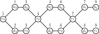
Figure 1: The network $G_{3}$

Lemma 35.

For every integer $x>1$, there is an execution of $RC(A)$ on $G_{x}$ that requires at least $2^{x}-1$ steps to reach a terminal configuration.

Proof.

Assume the following initial configuration $\gamma_{\text{init}}$:

• All nodes have 1 as input.

• For every $i\in[1..x]$,

  • $a_{i}.t=c_{i}.t=\overline{3(x-i)+1}$,

  • $d_{i}.t=\overline{3(x-i)+2}$, and

  • $b_{i}.t=e_{i}.t=\overline{3(x-i)+3}$.

Notice that the configuration is well-defined since all nodes has input 1 and a positive index; moreover the maximum index is $3(x-1)+3=3x$. (An example of possible initial configuration is given in Figure 1.)

We now show by induction on $i$ that for every $i\in[1..x]$, there is a prefix $P_{i}$ of execution starting from $\gamma_{\text{init}}$ and containing at least $2^{i}-1$ steps such that

• no node in $V(G_{x})\setminus V_{i}\cup\{c_{i}\}$ moves in $P_{i}$ and

• in the last configuration of $P_{i}$, noted $\gamma_{P_{i}}$, the index of all nodes $a_{j}$ with $j\in[1..i]$ have increased by 1 and no other index has changed.

For $i=1$, activating $a_{1}$ gives a prefix satisfying all requirements. Assume now $1<i\leq x$. We now explain how to expand the prefix $P_{i-1}$ given by the induction hypothesis. $P_{i-1}$ contains at least $2^{i-1}-1$ steps. Moreover,

• no node in $V(G_{x})\setminus V_{i-1}\cup\{c_{i-1}\}$ has ever moved in $P_{i-1}$ and

• the index of all nodes $a_{j}$ with $j\in[1..i-1]$ in $\gamma_{P_{i-1}}$ have increased by 1 and no other index has changed.

So, we should extend $P_{i-1}$ to reach at least $2^{i}-1$ steps while never activating a node in $V(G_{x})\setminus V_{i}\cup\{c_{i}\}$, moreover compared to $\gamma_{P_{i-1}}$, we should only increase the index of $a_{i}$ by one.

Consider the path $P=b_{i}c_{i-1}d_{i-1}e_{i-1}\cdots c_{2}d_{2}e_{2}c_{1}d_{1}e_{1}$ and the following scheduling of activation starting from $\gamma_{P_{i-1}}$.

1. Because the difference of indexes in $b_{i}$ and $a_{i}$ is 2, when activating $b_{i}$, its index decreases by 1. But then the difference of indexes in $c_{i-1}$ and $b_{i}$ becomes 2 which allows us to decrease the index of $c_{i-1}$. By activation the vertices of $P$ in order, all the indexes of the vertices of $P$ decrease by 1.

2. We can next activate all the vertices $a_{j}$ with $1\leq j<i$ which also decrease their index by 1.

3. We increase by 1 the index of $a_{i}$ by activating it.

4. We now activate all nodes of $P$, in order, to increase their index by 1.

Let $\gamma_{\text{half}}$ be the configuration reached after the previous scheduling. Compared to $\gamma_{\text{init}}$, only one index has changed: $a_{i}$. So, we re-apply the scheduling that has produced $P_{i-1}$. Let $\gamma_{\text{final}}$ be the reached configuration after applying this scheduling on $\gamma_{\text{half}}$. Compared to $\gamma_{\text{init}}$, the index of all nodes $a_{j}$ with $j\in[1..i]$ have increased by 1 and no other index has changed. Moreover, no node in $V(G_{x})\setminus V_{i}\cup\{c_{i}\}$ has moved in the prefix that led to $\gamma_{\text{final}}$. Finally, that prefix has length at least $(2^{i-1}-1)+1+(2^{i-1}-1)=2^{i}-1$. Thus, we can let $\gamma_{P_{i}}=\gamma_{\text{final}}$ and let $P_{i}$ be the prefix from $\gamma_{\text{init}}$ to $\gamma_{P_{i}}$ we have just exhibited. $P_{i}$ satisfies all requirements for $i$ and the induction holds. Finally, by letting $i=x$, the lemma holds. ∎∎

Corollary 1.

For every integer $x>1$, there is an execution of $RC(A)$ on $G_{x}$ that requires at least $2^{\frac{n}{5}}$ steps (resp. $2^{\frac{\mathcal{D}+1}{3}}$) to reach a terminal configuration, where $n$ is the number of nodes in (resp. $\mathcal{D}$ is the diameter of) $G_{x}$.

Assume the known upper bound on the time complexity of $A$ is not tight. We can let $x$ to obtain a network $G_{x}$ and arrays of with $T_{x}+1$ cells where $T_{x}$ is the known bound on the time complexity of $A$ on $G_{x}$. Then, we can add a node $z$ linked to all other nodes so that the diameter becomes 2. Finally, by considering a configuration identical to the previous construction, except that $z$ has a maximum index (i.e., $3x$), we can built the same execution (the presence of $z$ has no impact due its index). Hence, we can obtain an exponential lower bound that does not depend on the actual diameter but rather on the known upper bound.

11 Conclusion

We have proposed a versatile transformer that builds efficient silent self-stabilizing solutions. Precisely, our transformer achieves a good trade-off between time and workload since it allows to obtain fully-polynomial solutions with round complexities asymptotically linear in $D$ or even better.

Our transformer can be seen as a powerful tool to simplify the design of asynchronous self-stabilizing algorithms since it reduces the initial problem to the implementation of an algorithm just working in synchronous settings. By the way, all tasks, even non-self-stabilizing ones, that terminate in synchronous settings can be made self-stabilizing using our transformer, regardless the model in which they are written (atomic-state model, Local model, …).

Interestingly, the Local model which was initially devoted to prove lower bounds, becomes an upper bound provider since we can extensively use it to give inputs to our transformer that will, based on them, construct asymptotically time-optimal self-stabilizing solutions.

Another interesting application of our transformer is the weakening of fairness assumptions of silent self-stabilizing algorithms (e.g., asynchronous algorithms assuming a distributed weakly fair or a synchronous daemon) without compromising efficiency (actually, such algorithms can be provided as input of the transformer).

The perspectives of this work concern the space overhead and the moves complexity. The space overhead of our solution depends on the synchronous execution time of the input algorithm. In the spirit of the resynchronizer proposed by Awerbuch and Varghese [7], we may build another space-efficient transformer that would assume more constraint on input algorithms. Concerning the move complexity, for many problems, the trivial lower bound in moves for the asynchronous (silent) self-stabilization is $\Omega(D\times n)$; while we usually obtain upper bounds in $O(n^{3})$ moves with our transformer. Reduce the gap between those two bounds is another challenging perspective of our work.

References

- [1] Y. Afek and S. Dolev. Local stabilizer. Journal of Parallel and Distributed Computing, 62(5):745–765, 2002. doi:10.1006/jpdc.2001.1823.
- [2] Y. Afek, S. Kutten, and M. Yung. The local detection paradigm and its application to self-stabilization. Theoretical Computer Science, 186(1-2):199–229, 1997. doi:10.1016/S0304-3975(96)00286-1.
- [3] K. Altisen, A. Cournier, S. Devismes, A. Durand, and F. Petit. Self-stabilizing leader election in polynomial steps. Information and Computation, 254(3):330 – 366, 2017. doi:10.1016/j.ic.2016.09.002.
- [4] K. Altisen, S. Devismes, S. Dubois, and F. Petit. Introduction to Distributed Self-Stabilizing Algorithms. Synthesis Lectures on Distributed Computing Theory. Morgan & Claypool, 2019. doi:10.2200/S00908ED1V01Y201903DCT015.
- [5] D. Angluin. Local and global properties in networks of processors. In 12th Annual Symposium on Theory of Computing (STOC’80), pages 82–93, 1980. doi:10.1145/800141.804655.
- [6] B. Awerbuch, B. Patt-Shamir, and G. Varghese. Self-stabilization by local checking and correction. In 32nd Annual Symposium of Foundations of Computer Science (FOCS’91), pages 268–277, 1991. doi:10.1109/SFCS.1991.185378.
- [7] B. Awerbuch and G. Varghese. Distributed program checking: a paradigm for building self-stabilizing distributed protocols. In 32nd Annual Symposium on Foundations of Computer Science (FOCS’91), pages 258–267, 1991. doi:10.1109/SFCS.1991.185377.
- [8] S. Bernard, S. Devismes, M. Gradinariu Potop-Butucaru, and S. Tixeuil. Optimal deterministic self-stabilizing vertex coloring in unidirectional anonymous networks. In 23rd International Symposium on Parallel&Distributed Processing (IPDPS’09), pages 1–8, 2009. doi:10.1109/IPDPS.2009.5161053.
- [9] S. Bernard, S. Devismes, K. Paroux, M. Potop-Butucaru, and S. Tixeuil. Probabilistic self-stabilizing vertex coloring in unidirectional anonymous networks. In 11th International Conference on Distributed Computing and Networking (ICDCN’10), pages 167–177, 2010. doi:10.1007/978-3-642-11322-2_19.
- [10] L. Blin, P. Fraigniaud, and B. Patt-Shamir. On proof-labeling schemes versus silent self-stabilizing algorithms. In 16th International Symposium on Stabilization, Safety, and Security of Distributed Systems (SSS’14), pages 18–32, 2014. doi:10.1007/978-3-319-11764-5_2.
- [11] P. Boldi and S. Vigna. Universal dynamic synchronous self-stabilization. Distributed Computing, 15:137–153, 2002. doi:10.1007/s004460100062.
- [12] B. Chen, H. Yu, Y. Zhao, and P. B. Gibbons. The cost of fault tolerance in multi-party communication complexity. Journal of the ACM, 61(3):1–64, 2014. doi:10.1145/2597633.
- [13] R. Cole and U. Vishkin. Approximate and exact parallel scheduling with applications to list, tree and graph problems. In 27th Annual Symposium on Foundations of Computer Science (FOCS’86), pages 478–491, 1986. doi:10.1109/SFCS.1986.10.
- [14] A. Cournier, S. Devismes, and V. Villain. Light enabling snap-stabilization of fundamental protocols. ACM Transactions on Autonomous and Adaptive Systems, 4(1):1–27, 2009. doi:10.1145/1462187.1462193.
- [15] A. Cournier, S. Rovedakis, and V. Villain. The first fully polynomial stabilizing algorithm for bfs tree construction. Information and Computation, 265:26–56, 2019. doi:10.1016/j.ic.2019.01.005.
- [16] Dolev D. and R. Reischuk. Bounds on information exchange for byzantine agreement. In 1st Annual Symposium on Principles of Distributed Computing (PODC’82), pages 132–140, 1982. doi:10.1145/800220.806690.
- [17] A. K. Datta, S. Devismes, K. Heurtefeux, L. L. Larmore, and Y. Rivierre. Competitive self-stabilizing -clustering. Theoretical Computer Science, 626:110–133, 2016. doi:10.1016/j.tcs.2016.02.010.
- [18] A. K. Datta, S. Devismes, C. Johnen, and L. L. Larmore. Brief announcement: Analysis of a memory-efficient self-stabilizing BFS spanning tree construction. In 21th International Symposium on Stabilization, Safety, and Security of Distributed Systems (SSS’19, pages 99–104, 2019. doi:10.1007/978-3-030-34992-9_8.
- [19] A. K Datta, S. Devismes, and L. L. Larmore. A silent self-stabilizing algorithm for the generalized minimal -dominating set problem. Theoretical Computer Science, 753:35–63, 2019. doi:10.1016/j.tcs.2018.06.040.
- [20] A. K. Datta, L. L. Larmore, S. Devismes, K. Heurtefeux, and Y. Rivierre. Self-stabilizing small -dominating sets. International Journal of Networking and Computing, 3(1):116–136, 2013.
- [21] A. K. Datta, L. L. Larmore, and P. Vemula. An -time self-stabilizing leader election algorithm. Journal of Parallel and Distributed Computing, 71(11):1532–1544, 2011. doi:10.1016/j.jpdc.2011.05.008.
- [22] A. K. Datta, L. L. Larmore, and P. Vemula. Self-stabilizing leader election in optimal space under an arbitrary scheduler. Theoretical Computer Science, 412(40):5541–5561, 2011. doi:10.1016/j.tcs.2010.05.001.
- [23] S. Devismes, D. Ilcinkas, and C. Johnen. Optimized silent self-stabilizing scheme for tree-based constructions. Algorithmica, 84(1):85–123, 2022. doi:10.1007/s00453-021-00878-9.
- [24] S. Devismes and C. Johnen. Silent self-stabilizing bfs tree algorithms revisited. Journal on Parallel Distributed Computing, 97:11–23, 2016. doi:10.1016/j.jpdc.2016.06.003.
- [25] E. W. Dijkstra. Self-stabilization in spite of distributed control. Communications of the ACM, 17(11):643–644, 1974. doi:10.1145/361179.361202.
- [26] S. Dolev. Optimal time self stabilization in dynamic systems. In 7th International Workshop on Distributed Algorithms (WDAG’93), pages 160–173, 1993. doi:10.1007/3-540-57271-6_34.
- [27] S. Dolev. Self-Stabilization. MIT Press, 2000.
- [28] S. Dolev, M. G. Gouda, and M. Schneider. Memory requirements for silent stabilization. Acta Informatica, 36(6):447–462, 1999. doi:10.1007/s002360050180.
- [29] S. Dolev, A. Israeli, and S. Moran. Self-stabilization of dynamic systems assuming only read/write atomicity. Distributed Computing, 7(1):3–16, 1993. doi:10.1007/BF02278851.
- [30] Y. Emek and R. Wattenhofer. Stone age distributed computing. In 32nd Symposium on Principles of Distributed Computing, (PODC’13), pages 137–146, 2013. doi:10.1145/2484239.2484244.
- [31] M. J. Fischer, N. A. Lynch, and M. S. Paterson. Impossibility of distributed consensus with one faulty process. Journal of the ACM, 32(2):374–382, 1985. doi:10.1145/3149.214121.
- [32] C. Genolini and S. Tixeuil. A lower bound on dynamic -stabilization in asynchronous systems. In 21st Symposium on Reliable Distributed Systems (SRDS’02), pages 211–221, 2002. doi:10.1109/RELDIS.2002.1180190.
- [33] M. Gradinariu and S. Tixeuil. Self-stabilizing vertex coloration and arbitrary graphs. In 4th International Conference on Principles of Distributed Systems, (OPODIS’00), pages 55–70, 2000.
- [34] S. Huang and N. Chen. A self-stabilizing algorithm for constructing breadth-first trees. Information Processing Letters, 41(2):109–117, 1992. doi:10.1016/0020-0190(92)90264-V.
- [35] Cohen J., Pilard L., M. Rabie, and J. Sénizergues. Making self-stabilizing algorithms for any locally greedy problem. In 2nd Symposium on Algorithmic Foundations of Dynamic Networks, (SAND’23), volume 257, pages 1–17, 2023. doi:10.4230/LIPIcs.SAND.2023.11.
- [36] C. Johnen. Memory efficient, self-stabilizing algorithm to construct BFS spanning trees. In 16th Annual Symposium on Principles of Distributed Computing (PODC’97), page 288, 1997. doi:10.1145/259380.259508.
- [37] C. Johnen. Memory efficient self-stabilizing distance-k independent dominating set construction. In 3rd International Conference on Networked Systems, NETYS 2015, volume 9466, pages 354–366, 2015. doi:10.1007/978-3-319-26850-7_24.
- [38] S. Katz and K. J. Perry. Self-stabilizing extensions for message-passing systems. Distributed Computing, 7(1):17–26, 1993. doi:10.1007/BF02278852.
- [39] A. Kravchik and S. Kutten. Time optimal synchronous self stabilizing spanning tree. In 27th International Symposium on Distributed Computing, (DISC’13), volume 8205, pages 91–105, 2013. doi:10.1007/978-3-642-41527-2_7.
- [40] C. Lenzen, J. Suomela, and R. Wattenhofer. Local algorithms: Self-stabilization on speed. In 11th International Symposium on Stabilization, Safety, and Security of Distributed Systems (SSS’09), pages 17–34, 2009. doi:10.1007/978-3-642-05118-0_2.
- [41] N. Linial. Locality in distributed graph algorithms. SIAM Journal on Computing, 21(1):193–201, 1992. doi:10.1137/0221015.
- [42] S. Tixeuil. Vers l’auto-stabilisation des systèmes à grande échelle. Habilitation à diriger des recherches, Université Paris Sud - Paris XI, 2006. URL: https://tel.archives-ouvertes.fr/tel-00124848/file/hdr_final.pdf.
- [43] V. Turau. Efficient transformation of distance-2 self-stabilizing algorithms. Journal of Parallel and Distributed Computing, 72(4):603–612, 2012. doi:10.1016/j.jpdc.2011.12.008.