A well-balanced discontinuous Galerkin method for the first–order Z4 formulation of the Einstein–Euler system

Abstract

In this paper we develop a new well-balanced discontinuous Galerkin (DG) finite element scheme with subcell finite volume (FV) limiter for the numerical solution of the Einstein–Euler equations of general relativity based on a first order hyperbolic reformulation of the Z4 formalism. The first order Z4 system, which is composed of 59 equations, is analyzed and proven to be strongly hyperbolic for a general metric. The well-balancing is achieved for arbitrary but a priori known equilibria by subtracting a discrete version of the equilibrium solution from the discretized time-dependent PDE system. Special care has also been taken in the design of the numerical viscosity so that the well-balancing property is achieved. As for the treatment of low density matter, e.g. when simulating massive compact objects like neutron stars surrounded by vacuum, we have introduced a new filter in the conversion from the conserved to the primitive variables, preventing superluminal velocities when the density drops below a certain threshold, and being potentially also very useful for the numerical investigation of highly rarefied relativistic astrophysical flows.

Thanks to these improvements, all standard tests of numerical relativity are successfully reproduced, reaching three achievements: (i) we are able to obtain stable long term simulations of stationary black holes, including Kerr black holes with extreme spin, which after an initial perturbation return perfectly back to the equilibrium solution up to machine precision; (ii) a (standard) TOV star under perturbation is evolved in pure vacuum ($\rho=p=0$) up to $t=1000$ with no need to introduce any artificial atmosphere around the star; and, (iii) we solve the head on collision of two punctures black holes, that was previously considered un–tractable within the Z4 formalism.

1 Introduction

In spite of considerable progress made in the last two decades, the stable and accurate numerical solution of the Einstein field equations still remains an extremely challenging task to be tackled. Among recent achievements, we highlight the results obtained in [107, 120, 108, 129, 118, 139]. One of the primary obstacles for numerical discretization of the Einstein equations is the fact that these equations are not immediately well-posed in their original four-dimensional form, and a well-posed 3+1 formulation is required. On a mathematical ground, the well-posedness of a 3+1 formulation of the Einstein equations would be guaranteed if one could prove that such a system of time-dependent partial differential (PDE) equations is unconditionally symmetric hyperbolic [38, 130, 39, 132]. However, there are a number of reasons which prevent from reaching a simple conclusion in this respect. First, the Einstein equations arise as nonlinear second order PDEs in the metric coefficients, and reducing them to a first–order system from which the required mathematical properties can emerge more clearly is far from trivial [89]. Second, the gauge freedom which is inherent to the Einstein equations is quite often a rather delicate issue, as it can substantially affect hyperbolicity [76]. Finally, as the Einstein equations include a set of stationary nonlinear second order differential constraints which must be satisfied during the evolution, their proper treatment can also have important implications on the mathematical nature of the overall PDE system.

Despite the symmetric hyperbolicity being necessary for strictly proving well-posedness of a given first–order PDE system, from the computational view point this condition might be slightly relaxed as it is well known that for stable numerical computations, in fact, a strongly hyperbolic formulation is usually enough. In particular, the first-order strongly hyperbolic 3+1 formulation used in this paper does not have an obvious symmetric hyperbolic reformulation, at least to the best of our knowledge. Yet, it provides the possibility to perform stable computations of the Einstein field equations. We note that several symmetric hyperbolic formulations of the Einstein's equations in 3+1 split are known [76, 2, 71, 8, 29, 94], but the applicability of most of these formulations in numerical general relativity (GR) has yet to be tested.

One can notice that, after the first detection of gravitational waves recorded in 2015 [1], the vast majority of research groups performing numerical simulations of the gravitational signal from astrophysical sources have been adopting the so called 3+1 formalism [3] in its various formulations. Some representative examples include [14, 92, 95, 108, 115, 33, 54]. In many of these codes the amount of physical effects that are currently taken into account is really impressive (see [13] for a review). The most popular and successful implementations using the 3+1 foliation of spacetime include the BSSNOK (Baumgarte-Shapiro-Shibata-Nakamura-Oohara-Kojima) formulation [134, 16, 114, 27]; the Z4 formulation of [21, 22, 5], which has the advantage of incorporating the treatment of the Einstein constraints through the addition of a four vector $z^{\mu}$; the Z4c formulation [20], which adds a conformal transformation to the metric; the CCZ4 formulation of [6, 7], where suitable coefficients are added to damp the violation of the Einstein constraints and it is particularly suitable for treating binary systems. Finally, in recent work [59, 58] a first–order version of CCZ4 was proposed, namely FO-CCZ4, which consists of a system of 59 equations, it is strongly hyperbolic for a particular choice of gauges and it incorporates a curl-cleaning technique for the treatment of internal curl-free conditions. As a proper mathematical formulation of the Einstein equations must be accompanied by a good numerical scheme in order to obtain stable and accurate numerical simulations, in [59, 58] a numerical scheme based on discontinuous Galerkin methods combined with finite volume subcell limiter [64] was used.

In spite of their attractive features in terms of accuracy and scalability on parallel computers, DG methods are far from common in the relativistic framework. After the pioneering investigations of [68, 128], and apart from a slightly better popularity for treating relativistic flows in stationary spacetimes, with or without magnetic fields [31, 145, 53, 51, 84], their usage in full numerical relativity remains rather limited, with only a few groups investing on them around the world [137, 111, 100, 93, 139]. While in the just mentioned works the time evolution is performed via Runge–Kutta schemes at various orders, the approach followed by our group over the years has been to resort to ADER (arbitrary high order derivatives) schemes [140, 141], which incorporate the solution of a Generalized Riemann Problem (GRP) at the cell boundaries. After the modern reformulation of ADER provided by [57, 65], where the approximate solution of the GRP is obtained by evolving the data inside each cell through a local space-time discontinuous Galerkin predictor, ADER schemes have been successfully implemented to solve the relativistic hydrodynamics and magnetohydrodynamics equations in stationary spacetimes [146, 147, 149, 73, 81]. With the present work, we resume our investigations in full numerical relativity with DG methods, by revisiting the original Z4 formulation of the Einstein equations, which, as we clarify below, does not show any inconvenience with respect to the CCZ4 formulation and is significantly simpler.

In addition, when one performs numerical simulations of (nearly) stationary configurations, a crucial property that ought to be achieved is the ability to preserve equilibria exactly at the discrete level over long time scales. Indeed, this capability, besides guaranteeing long-time stable simulations of the equilibrium profiles themselves, allows to capture with increased accuracy small physical perturbations around them that otherwise would be hidden by spurious numerical oscillations. For instance, this is particularly relevant when studying normal modes of oscillations in relativistic astrophysical sources [105, 75]. Thus, in this work we endow our high order finite volume and discontinuous Galerkin schemes with so-called well-balanced (WB) techniques. Such techniques were originally introduced in computational fluid dynamics for the shallow water equations, see e.g. [18, 104, 86, 26, 12, 34, 116, 117], and then successfully employed for many different applications with a number of relevant results over the last two decades [35, 110, 82, 78, 11, 36, 123]. In particular, there has been a major interest for well-balancing in astrophysical applications, starting from their use joint to the classical Newtonian Euler equations with gravity, see for example [25, 96, 97, 37, 19, 79, 37, 52, 101, 138, 88] to the more recent work of [80], where WB has been applied for the first time to the relativistic framework allowing the (1D) numerical simulations of the coupled evolution of matter and spacetime for small perturbations of neutron star equilibrium configurations. In this work we propose a new, simple but rather efficient approach to obtain the well-balanced property inside an existing three-dimensional general purpose code for numerical general relativity that is based on finite volume and discontinuous Galerkin finite element schemes and which includes also adaptive mesh refinement (AMR) with time-accurate local time stepping (LTS), see [63, 146, 59]. Our new kind of well-balancing can be easily applied even to very complex hyperbolic PDE systems, such as the Einstein field equations, for which the original WB algorithm of [34, 80] becomes more cumbersome, in particular when combining DG and FV schemes inside a 3D AMR framework with LTS.

The structure of the paper is the following: in Sect. 2 we present the original Z4 formulation provided by [21, 22, 24] with only minor modifications. Sect. 3 is devoted to the description of the new well-balanced ADER-DG scheme with subcell finite volume limiter, while Sect. 4 contains the results of our investigations. Finally, we conclude our analysis in Sect. 5 with a few indications for further progresses.

Throughout this paper we assume a signature $(-,+,+,+)$ for the spacetime metric and we will use Greek letters (running from $0$ to $3$) for four-dimensional spacetime tensor components, while Latin letters (running from $1$ to $3$) for three-dimensional spatial tensor components. Moreover, we adopt a geometrized system of units by setting $c=G=1$, in such a way that the most convenient unit of lengths is $r_{g}=G\,M/c^{2}=M$. We just recall that for a one solar mass black hole, this choice corresponds to $r_{g}=1.476\times 10^{3}\,{\text{m}}$ as a unit of length and to $r_{g}=4.925\times 10^{-6}\,{\text{s}}$ as a unit of time.

2 Damped Z4 formulation of the Einstein equations

2.1 The 3+1 splitting of spacetime

According to the 3+1 formalism, the spacetime can be foliated through $\Sigma_{t}=const$ hypersurfaces as

$$ds^{2}=-(\alpha^{2}-\beta_{i}\beta^{i})dt^{2}+2\beta_{i}dx^{i}dt+\gamma_{ij}dx^{i}dx^{j}\,,$$ (1)

where $\alpha$ is the lapse, $\beta^{i}$ is the shift and $\gamma_{ij}$ is the metric of the three dimensional space, see [3, 131, 17, 87] for an extended discussion. An Eulerian observer is then introduced, with four velocity defined by $n^{\mu}=\frac{1}{\alpha}(1,-\beta^{i})$ everywhere orthogonal to the hypersurface $\Sigma_{t}$, and with respect to whom all physical quantities are measured. In the following, the spatial covariant derivative is denoted by $\nabla_{i}$. We recall that the original Z4 formulation of the Einstein equations was not meant to be restricted to the 3+1 formalism. In fact, it was specifically devised by [21, 22] to hyperbolize the elliptic Einstein constraints in a general covariant framework, after introducing an additional quantity $z^{\mu}$ whose role is analogous to the scalar $\Psi$ in the divergence cleaning approach of [112, 49] for the Maxwell and magnetohydrodynamics equations. On the other hand, the damped version of the Z4 formulation, first proposed by [90], was intrinsically linked to the 3+1 framework, since it dragged the four vector $n^{\mu}$ directly into the Einstein equations, in combination with two additional constant coefficients $\kappa_{1}$ and $\kappa_{2}$, which were introduced to allow for the damping of the four vector $z^{\mu}$ as it propagates constraint violations away. An alternative rigorous treatment of the constraints is obtained via so-called fully-constrained formulations, see e.g. [45, 44] and references therein.

Here we introduce a slightly different version with respect to [90], where the coefficients $\kappa_{1}$ and $\kappa_{2}$ are never multiplied among each other and thus produce effects that are clearly separated. Hence the augmented Einstein equations with damped Z4 cleaning read

$$G_{\mu\nu}+\nabla_{\mu}z_{\nu}+\nabla_{\nu}z_{\mu}-\nabla_{\pi}z^{\pi}g_{\mu\nu}-\kappa_{1}(n_{\mu}z_{\nu}+n_{\nu}z_{\mu})-\kappa_{2}n_{\pi}z^{\pi}g_{\mu\nu}=8\pi T_{\mu\nu}\,,$$ (2)

or, equivalently,

$${{}^{{}^{(4)}}}R_{\mu\nu}+\nabla_{\mu}z_{\nu}+\nabla_{\nu}z_{\mu}-\kappa_{1}(n_{\mu}z_{\nu}+n_{\nu}z_{\mu}-n_{\pi}z^{\pi}g_{\mu\nu})+\kappa_{2}n_{\pi}z^{\pi}g_{\mu\nu}=8\pi\left(T_{\mu\nu}-\frac{1}{2}Tg_{\mu\nu}\right)\,,$$ (3)

where $G_{\mu\nu}$ and ${{}^{{}^{(4)}}}R_{\mu\nu}$ are the Einstein and the Ricci tensors, while $T^{\mu\nu}$ is the energy–momentum tensor of matter. In this paper we limit our attention to a perfect fluid with no magnetic fields, such that

$$T^{\mu\nu}=(e+p)u^{\mu}u^{\nu}+pg^{\mu\nu}=\rho hu^{\mu}u^{\nu}+pg^{\mu\nu}\,,$$ (4)

with $e$, $p$, $\rho$ and $h$ being the energy density, the pressure, the rest mass density and the specific enthalpy, respectively, each of them measured in the comoving frame of the fluid with four velocity $u^{\mu}$. We notice that the wave equation for the four vector $z^{\mu}$ corresponding to (2) is

$$\nabla^{\mu}\nabla_{\mu}z_{\nu}+R_{\mu\nu}z^{\mu}=\kappa_{1}\nabla^{\mu}(n_{\mu}z_{\nu}+n_{\nu}z_{\mu})+\kappa_{2}\nabla_{\nu}(n_{\rho}z^{\rho})\,,$$ (5)

which is obtained after taking the four divergence of (2). Within the 3+1 decomposition, all vectors and tensors are split in their components parallel and perpendicular (or mixed, depending on the rank) to $n^{\mu}$. So, for instance, we have

$$u^{\,\mu} = W\,n^{\,\mu}+W\,v^{\,\mu},$$ (6)

$$T^{\mu\nu} = S^{\mu\nu}+S^{\mu}n^{\nu}+n^{\,\mu}S^{\nu}+En^{\,\mu}n^{\nu},$$ (7)

$$z^{\mu} = \Theta n^{\mu}+Z^{\mu},$$ (8)

where $W=-u^{\mu}n_{\mu}=1/\sqrt{1-v^{2}}$ is the Lorentz factor of the fluid, $S_{\mu\nu}=\gamma^{\alpha}_{\mu}\,\gamma^{\beta}_{\nu}T_{\alpha\beta}$ is the spatial part of the energy–momentum tensor, $S_{\mu}=-\gamma^{\alpha}_{\mu}\,n^{\beta}T_{\alpha\beta}$ is the momentum density, $\gamma^{\mu}_{\nu}=n^{\mu}n_{\nu}+\delta^{\mu}_{\nu}$ is the spatial projector tensor, $\delta^{\mu}_{\nu}$ is the Kronecker delta, $E=n^{\alpha}\,n^{\beta}T_{\alpha\beta}$ is the energy density, $Z^{\mu}=\gamma^{\mu}_{\nu}z^{\nu}$ is the purely spatial part of the four vector $z^{\mu}$ and $\Theta=-z^{\mu}n_{\mu}=\alpha z^{0}$, each of which is measured in the Eulerian observer frame. In terms of the primitive variables they read

$$S^{\mu\nu} =\rho hW^{2}v^{\mu}v^{\nu}+p\gamma^{\mu\nu}\,,$$ (9)

$$S^{\mu} =\rho hW^{2}v^{\mu}\,,$$ (10)

$$E =\rho hW^{2}-p\,.$$ (11)

There are also vectors and tensors which are intrinsically spatial, namely without any component along $n^{\mu}$, such as the four acceleration of the Eulerian observer

$$a^{\mu}=n^{\nu}\nabla_{\nu}n^{\mu}=\gamma^{\mu\nu}\nabla_{\nu}\ln\alpha\,,$$ (12)

or the extrinsic curvature of the hypersurface $\Sigma_{t}$, a symmetric tensor defined as

$$K_{\mu\nu}=-\gamma^{\alpha}_{\mu}\nabla_{\alpha}n_{\nu}=-\nabla_{\mu}n_{\nu}-n_{\mu}a_{\nu}\,,$$ (13)

which plays a fundamental role as a dynamical set of quantities, representing the opposite of the (non–trace-free) shear tensor of the Eulerian four velocity $n^{\mu}$. We notice that the purely spatial part of the Ricci tensor $R_{\mu\nu}$ is not simply given by the full spatial projection of the four dimensional Ricci tensor ${{}^{{}^{(4)}}}R^{\mu\nu}$, but rather is obtained from the so-called contracted Gauss relations, i.e.

$$R_{\mu\nu}=\gamma^{\alpha}_{\mu}\gamma^{\beta}_{\nu}\,\,{{}^{{}^{(4)}}}R_{\alpha\beta}+\gamma^{\alpha}_{\mu}\gamma^{\beta}_{\nu}n^{\sigma}n^{\pi}\,\,{{}^{{}^{(4)}}}R_{\alpha\sigma\beta\pi}-KK_{\mu\nu}+K_{\mu\pi}K^{\pi}_{\,\,\nu}\,,$$ (14)

where $K=\gamma^{ij}K_{ij}=-\nabla_{\mu}n^{\mu}$ is the trace of the extrinsic curvature, also equal to the opposite of the Eulerian observer expansion.

2.2 The second order Z4 system

The second order PDE system that governs the evolution of the gravitational field in the presence of matter is given by (see also  [21] for a comparison)

$$(\partial_{t}-{\cal L}_{\beta})\leavevmode\nobreak\ \gamma_{ij} = -{2\,\alpha}\,K_{ij}$$ (15)

$$(\partial_{t}-{\cal L}_{\beta})\leavevmode\nobreak\ K_{ij} = -\nabla_{i}\nabla_{j}\alpha+\alpha\,\bigg{[}R_{ij}+\nabla_{i}Z_{j}+\nabla_{j}Z_{i}-\kappa_{1}\Theta\gamma_{ij}-\kappa_{2}\Theta\gamma_{ij}-2\Theta K_{ij}$$ (16)

$$- 2K_{im}K^{m}_{j}+K\,K_{ij}-8\pi\left(S_{ij}-\frac{1}{2}\,T\,\gamma_{ij}\right)\,\bigg{]}$$

$$(\partial_{t}-{\cal L}_{\beta})\leavevmode\nobreak\ \Theta = \frac{\alpha}{2}\,e^{2}\left[R+K^{2}-K_{ij}\,K^{ij}-16\pi\,E\right]+\alpha\left[\nabla_{k}Z^{k}-Z^{k}\frac{\nabla_{k}\alpha}{\alpha}-\Theta(2\kappa_{1}+\kappa_{2})-K\Theta\right]$$ (17)

$$(\partial_{t}-{\cal L}_{\beta})\leavevmode\nobreak\ Z_{i} = \alpha\,\left[\nabla_{j}\,{K_{i}}^{j}-\nabla_{i}\,K-8\pi S_{i}\right]+\alpha[\partial_{i}\Theta-2\,{K_{i}}^{j}\,Z_{j}-\Theta\,\nabla_{i}\ln\alpha-\kappa_{1}Z_{i}]\,.$$ (18)

Furthermore, we stress the following facts about each of the above equations. Eq. (15) is a pure relation coming from differential geometry and which can be derived without any reference to the Einstein field equations. It states that the dynamics of the spatial metric tensor $\gamma_{ij}$ is determined by the extrinsic curvature. Eq. (16) is obtained after inserting the four dimensional Ricci tensor as given by the Einstein equation (3) into the so–called Ricci equation of differential geometry (see [17, 131] for an extended discussion). Finally, Eqs. (17)–(18) are the evolutionary version of the Einstein constraints within the Z4 formalism and are obtained after contracting the Einstein equations (3) with $n^{\mu}n^{\nu}$ and $n^{\mu}\gamma^{\nu}_{\pi}$, respectively. In fact, the Hamiltonian constraint $H$ and the momentum constraints $M_{i}$, defined as

$$H = R-K_{ij}K^{ij}+K^{2}-16\pi E\,,$$ (19)

$$M_{i} = \gamma^{jl}\left(\partial_{l}K_{ij}-\partial_{i}K_{jl}-\Gamma^{m}_{jl}K_{mi}+\Gamma^{m}_{ji}K_{ml}\right)-8\pi S_{i}\,,$$ (20)

can be recognized on the right hand side of (17) and (18). Assumed to be zero for proper initial data of the Einstein equations, on the discrete level such quantities can in fact increase, and the whole strategy of the Z4 approach is to keep their dynamics under control by tranporting the numerical erros away from the computational domain at the velocity $e$, which is the so-called cleaning speed.

2.3 The first–order Z4 system with matter

Similarly to the standard approach of [21, 22, 59], we introduce 30 auxiliary variables involving first derivatives of the metric terms, namely

$$A_{i}:=\partial_{i}\ln\alpha=\frac{\partial_{i}\alpha}{\alpha}\,,\qquad B_{k}^{\,\,i}:=\partial_{k}\beta^{i}\,,\qquad D_{kij}:=\frac{1}{2}\partial_{k}\gamma_{ij}\,.\qquad$$ (21)

In addition, we list the following expressions and identities, clarifying how second order spatial derivatives can be removed:

$${\gamma} = \textnormal{det}({\gamma}_{ij})\,,$$ (22)

$$\partial_{k}{\gamma}^{ij} = -2{\gamma}^{in}{\gamma}^{mj}D_{knm}\,,$$ (23)

$$\Gamma_{ij}^{k} = {\gamma}^{kl}\left(D_{ijl}+D_{jil}-D_{lij}\right)\,,$$ (24)

$$\partial_{k}\Gamma_{ij}^{m} = -2{\gamma}^{mn}{\gamma}^{pl}D_{knp}\left(D_{ijl}+D_{jil}-D_{lij}\right)+{\gamma}^{ml}\left(\partial_{(k}{D}_{i)jl}+\partial_{(k}{D}_{j)il}-\partial_{(k}{D}_{l)ij}\right),$$ (25)

$$R^{m}_{\,\,ikj} = \partial_{k}\Gamma^{m}_{ij}-\partial_{j}\Gamma^{m}_{ik}+\Gamma^{m}_{lk}\,\Gamma^{l}_{ij}-\Gamma^{m}_{lj}\,\Gamma^{l}_{ik},$$ (26)

$$R_{ij} = R^{k}_{\,\,ikj}=\partial_{k}\Gamma^{k}_{ij}-\partial_{j}\Gamma^{k}_{ik}+\Gamma^{k}_{lk}\,\Gamma^{l}_{ij}-\Gamma^{k}_{lj}\,\Gamma^{l}_{ik}\,,$$ (27)

$$R = \gamma^{ij}\,R_{ij}\,,$$ (28)

$$\nabla_{i}\nabla_{j}\alpha = \alpha A_{i}A_{j}-\alpha\,\Gamma^{k}_{ij}A_{k}+\alpha\partial_{(i}{A}_{j)}\,,$$ (29)

$${\Gamma}^{i} = {\gamma}^{jk}\,{\Gamma}^{i}_{jk}\,,$$ (30)

$$\partial_{k}{\Gamma}^{i} = -2D_{k}^{jl}\,\Gamma^{i}_{jl}+{\gamma}^{jl}\,\partial_{k}\Gamma^{i}_{jl}\,.$$ (31)

Having done that, we can rephrase the system (15)–(18) as a first–order system, augmented by the matter part (see [50] for details). The full Z4 Einstein-Euler system is therefore given by

$$\partial_{t}(\sqrt{\gamma}D)+\partial_{i}\left[\sqrt{\gamma}(\alpha v^{i}D-\beta^{i}D)\right]=0\,,$$ (32)

$$\partial_{t}(\sqrt{\gamma}S_{j})+\partial_{i}\left[\sqrt{\gamma}(\alpha S^{i}_{\,\,j}-\beta^{i}S_{j})\right]=\sqrt{\gamma}\left[\frac{1}{2}\alpha S^{ik}\partial_{j}\gamma_{ik}+S_{i}\partial_{j}\beta^{i}-E\partial_{j}\alpha\right]\,,$$ (33)

$$\partial_{t}(\sqrt{\gamma}E)+\partial_{i}\left[\sqrt{\gamma}(\alpha S^{i}-\beta^{i}E)\right]=\sqrt{\gamma}\left[\alpha S^{ij}K_{ij}-S^{j}\partial_{j}\alpha\right]\,,$$ (34)

$$\partial_{t}\gamma_{ij}-\beta^{k}\partial_{k}\gamma_{ij}=\gamma_{ik}B_{j}^{\,\,k}+\gamma_{kj}B_{i}^{\,\,k}-2\alpha K_{ij}\,,$$ (35)

$$\partial_{t}K_{ij}-\beta^{k}\partial_{k}K_{ij}+\alpha\partial_{(i}{A}_{j)}-\alpha{\gamma}^{kl}\left(\partial_{(k}{D}_{i)jl}-\partial_{(k}{D}_{l)ij}\right)+\alpha{\gamma}^{kl}\left(\partial_{(j}{D}_{i)kl}-\partial_{(j}{D}_{l)ik}\right)-2\alpha\partial_{(i}{Z}_{j)}=K_{ki}B_{j}^{\,\,k}+K_{kj}B_{i}^{\,\,k}$$

$$-\alpha A_{i}A_{j}+\alpha\Gamma^{k}_{ij}A_{k}+\alpha\bigg{[}-2{\gamma}^{kn}{\gamma}^{pl}D_{knp}\left(D_{ijl}+D_{jil}-D_{lij}\right)+2{\gamma}^{kn}{\gamma}^{pl}D_{jnp}\left(D_{ikl}+D_{kil}-D_{lik}\right)$$

$$+\Gamma^{m}_{lm}\Gamma^{l}_{ij}-\Gamma^{m}_{lj}\Gamma^{l}_{im}\bigg{]}-2\alpha\Gamma^{k}_{ij}Z_{k}-\alpha\Theta\gamma_{ij}(\kappa_{1}+\kappa_{2})-2\alpha K_{il}\gamma^{lm}K_{mj}+\alpha K_{ij}(K-2\Theta)$$

$$-8\pi\alpha\left(S_{ij}-\frac{1}{2}\,T\,\gamma_{ij}\right)\,,$$ (36)

$$\partial_{t}\Theta-\beta^{k}\partial_{k}\Theta-\frac{1}{2}\alpha{e^{2}}\left[\gamma^{ij}{\gamma}^{kl}\left(\partial_{(k}{D}_{i)jl}-\partial_{(k}{D}_{l)ij}\right)-\gamma^{ij}{\gamma}^{kl}\left(\partial_{(j}{D}_{i)kl}-\partial_{(j}{D}_{l)ik}\right)+2\gamma^{ij}\partial_{i}Z_{j}\right]=$$

$$=\frac{\alpha}{2}\,e^{2}\,\bigg{[}-2\gamma^{ij}{\gamma}^{kn}{\gamma}^{pl}D_{knp}\left(D_{ijl}+D_{jil}-D_{lij}\right)+2\gamma^{ij}{\gamma}^{kn}{\gamma}^{pl}D_{jnp}\left(D_{ikl}+D_{kil}-D_{lik}\right)$$

$$+\gamma^{ij}\left(\Gamma^{m}_{lm}\Gamma^{l}_{ij}-\Gamma^{m}_{lj}\Gamma^{l}_{im}\right)+K^{2}-K_{ij}\,K^{ij}-16\pi\,E\bigg{]}+\alpha\left[-\gamma^{ij}\,\Gamma^{k}_{ij}Z_{k}-Z^{k}A_{k}\right]$$

$$-\alpha\Theta K-\alpha\Theta(2\kappa_{1}+\kappa_{2})\,,$$ (37)

$$\partial_{t}Z_{i}-\beta^{k}\partial_{k}Z_{i}-\alpha\partial_{i}\Theta-\alpha\left[\gamma^{jm}\partial_{j}K_{mi}-\gamma^{mn}\partial_{i}K_{mn}\right]=Z_{k}\,B_{i}^{\,\,k}+\alpha\,\bigg{[}-\gamma^{jm}(\Gamma^{n}_{jm}K_{ni}+\Gamma^{n}_{ji}K_{mn})$$

$$+\gamma^{mn}(\Gamma^{l}_{im}K_{ln}+\Gamma^{l}_{in}K_{ml})-8\pi S_{i}\bigg{]}+\alpha[-2\,{K_{i}}^{j}\,Z_{j}-\Theta\,A_{i}-\kappa_{1}Z_{i}]\,,$$ (38)

where we have written the principal part of the PDEs on the left hand side, while moving all algebraic source terms to the right. In addition to the system (32)–(2.3), we need to adopt specific gauge conditions, which we choose in the following way. For the lapse, we assume the standard form [17]

$$\partial_{t}\ln\alpha-\beta^{k}{\partial_{k}\ln\alpha}=-g(\alpha)\alpha(K-K_{0}-2c\Theta)\,,$$ (39)

which gives us the possibility to switch among the 1+log gauge condition, setting $g(\alpha)=2/\alpha$, and the harmonic gauge condition, setting $g(\alpha)=1$. For the shift, on the other hand, we use the gamma–driver condition in those cases when the evolution of the shift is needed, and in particular we adopt the so-called ``non–shifting–shift" version of [72]

$$\partial_{t}\beta^{i} = \frac{3}{4}b^{i},$$ (40)

$$\partial_{t}b^{i} = \partial_{t}\hat{\Gamma}^{i}-\eta b^{i}\,,$$ (41)

where $\hat{\Gamma}^{i}=\Gamma^{i}+2\gamma^{ij}Z_{j}$ and $\Gamma^{i}=\gamma^{jk}\,\Gamma^{i}_{jk}$. Note that the quantities $\hat{\Gamma}^{i}$ are not primary variables, and their time evolution can be deduced from the other dynamical variables as specified below. From the gauge conditions (39)–(40) we can then obtain the PDEs for the auxiliary variables, namely

$$\partial_{t}A_{i}-{\beta^{k}\partial_{k}A_{i}}+\alpha g(\alpha)\left(\gamma^{mn}\partial_{i}K_{mn}-\partial_{i}K_{0}-2c\partial_{i}\Theta\right)=-\alpha A_{i}\left(K-K_{0}-2\Theta c\right)\left(g(\alpha)+\alpha g^{\prime}(\alpha)\right)+$$

$$+\partial_{i}\gamma^{mn}K_{mn}+B_{i}^{\,\,k}\leavevmode\nobreak\ A_{k}\,,$$ (42)

$$\partial_{t}B_{k}^{\,\,i}-s\left(\frac{3}{4}\partial_{k}b^{i}-\alpha^{2}\mu\,\gamma^{ij}\gamma^{nl}\left(\partial_{k}D_{ljn}-\partial_{l}D_{kjn}\right)\right)=0\,,$$ (43)

$$\partial_{t}D_{kij}-{\beta^{l}\partial_{l}D_{kij}}-\frac{1}{2}{\gamma}_{mi}\partial_{(k}{B}_{j)}^{m}-\frac{1}{2}{\gamma}_{mj}\partial_{(k}{B}_{i)}^{m}+\alpha\partial_{k}{K}_{ij}=B_{k}^{\,\,m}D_{mij}+B_{j}^{\,\,m}D_{kmi}+B_{i}^{\,\,m}D_{kmj}$$

$$-\alpha A_{k}{K}_{ij}\,.$$ (44)

The following aspects ought to be emphasized about the whole system (32)–(2.3)

• The first five equations for the evolution of matter are in conservative form, while the rest of the equations are in non conservative form.

• The quantities $\hat{\Gamma}^{i}$ in Eq. (41) are not primary variables. Their evolution in time is obtained from

  $$\partial_{t}\hat{\Gamma}^{i}=\partial_{t}\gamma^{jk}\,\,\Gamma^{i}_{jk}+\gamma^{jk}\,\,\partial_{t}\Gamma^{i}_{jk}+2\left(Z_{j}\partial_{t}\gamma^{ij}+\gamma^{ij}\partial_{t}Z_{j}\right)\,,$$ (45)

  which involve time derivatives of the already existing dynamical variables. In fact, we can write

  $$\partial_{t}\gamma^{ij} = -\gamma^{in}\gamma^{jm}\partial_{t}\gamma_{nm}$$ (46)

  $$= -2\gamma^{in}\gamma^{jm}\beta^{r}\,D_{rnm}-\gamma^{jm}B_{m}^{\,\,i}-\gamma^{in}B_{n}^{\,\,j}+2\alpha\gamma^{in}\gamma^{jm}K_{nm},$$

  $$\partial_{t}\Gamma^{i}_{jk} = \partial_{t}\gamma^{im}\left(D_{jmk}+D_{kjm}-D_{mjk}\right)+\gamma^{im}\left(\partial_{t}D_{jmk}+\partial_{t}D_{kjm}-\partial_{t}D_{mjk}\right)$$ (47)

  $$= \gamma^{im}\beta^{r}\left[\partial_{r}D_{jmk}+\partial_{r}D_{kjm}-\partial_{r}D_{mjk}\right]+\partial_{(j}B_{k)}^{\,\,i}-\alpha\gamma^{im}\left(\partial_{j}K_{mk}+\partial_{k}K_{jm}-\partial_{m}K_{jk}\right)+$$

  $$+\gamma^{im}\big{[}D_{jmn}B_{k}^{\,\,n}+D_{nmk}B_{j}^{\,\,n}+D_{knm}B_{j}^{\,\,n}+D_{njm}B_{k}^{\,\,n}-D_{mjn}B_{k}^{\,\,n}-D_{mnk}B_{j}^{\,\,n}\big{]}$$

  $$-\alpha\gamma^{im}\left(A_{j}K_{mk}+A_{k}K_{jm}-A_{m}K_{jk}\right)+$$

  $$+\big{[}-2\gamma^{ip}\gamma^{mq}\beta^{r}D_{rpq}-\gamma^{mr}B_{r}^{\,\,i}+2\alpha\gamma^{ip}\gamma^{mq}K_{pq}\big{]}\left(D_{jmk}+D_{kjm}-D_{mjk}\right).$$

• The binary parameter $s$ in Eq. (43)–(2.3), either 1 or 0, is introduced to switch the gamma–driver on or off, depending on the test being considered.

The equations (32)–(2.3) above form a non-conservative first-order hyperbolic system, namely they can be written as

$$\frac{\partial\mathbf{u}}{\partial t}+\frac{\partial\mathbf{f}_{i}(\mathbf{u})}{\partial x_{i}}+\mathbf{B}_{i}(\mathbf{u})\frac{\partial\mathbf{u}}{\partial x_{i}}=\mathbf{S}(\mathbf{u}),\qquad\textnormal{or, equivalently,}\qquad\frac{\partial\mathbf{u}}{\partial t}+\nabla\cdot\mathbf{F}(\mathbf{u})+\mathbf{B}(\mathbf{u})\cdot\nabla\mathbf{u}=\mathbf{S}(\mathbf{u}),$$ (48)

where $\mathbf{u}$ is the state vector, composed of 59 dynamical variables, ${\bf F}(\mathbf{u})=(\mathbf{f}_{1}(\mathbf{u}),\mathbf{f}_{2}(\mathbf{u}),\mathbf{f}_{3}(\mathbf{u}))$ is the flux tensor for the conservative (hydrodynamic) part of the PDE system, while ${\mathbf{B}}(\mathbf{u})=\left(\mathbf{B}_{1}(\mathbf{u}),\mathbf{B}_{2}(\mathbf{u}),\mathbf{B}_{3}(\mathbf{u})\right)$ represents the non-conservative part of the system, essentially all of the Einstein sector. Finally, $\bf S(\mathbf{u})$ is the source term, which contains algebraic terms only. When written in pure quasilinear form, the system (48) becomes

$$\frac{\partial\mathbf{u}}{\partial t}+{\bm{A}}_{i}(\mathbf{u})\frac{\partial\mathbf{u}}{\partial x_{i}}=\textbf{S}(\mathbf{u})\,,$$ (49)

where the matrix ${\bf A}_{i}(\mathbf{u})=\partial{\bf f}_{i}(\mathbf{u})/\partial\mathbf{u}+{\bf B}_{i}(\mathbf{u})$ contains both the conservative and the non-conservative contributions. Sect. 3 below describes the numerical methods adopted to solve such a system of equations.

2.4 Hyperbolicity of the first order Z4 system

Even before the Z4 formalism was introduced, in [23] the hyperbolic nature of the first–order conservative formulation of the Einstein field equations was highlighted. It was subsequently confirmed after the introduction of the Z4 approach [21]. However, our analysis differs from theirs, since our system (32)–(2.3) is written in non–conservative form. In the context of the CCZ4 formulation [66, 59], we have already emphasized that the hyperbolicity of a system like (49) is favoured if one makes the maximum possible use of the auxiliary variables defined in Eq. (21). In other words, our first-order Z4 system does not contain any spatial derivatives of $\alpha$, $\beta^{i}$, ${\gamma}_{ij}$, which have been moved to the purely algebraic source term $\bm{S}(\mathbf{u})$ precisely by using the auxiliary quantities defined in (21). We have verified the hyperbolicity of the subsystem (35)–(2.3) governing the space-time evolution by computing the eigenvalues and the corresponding eigenvectors through the symbolic mathematical software Maple. The results for a general metric are reported in  A.

3 The numerical scheme

3.1 A well-balanced ADER-DG scheme for non conservative systems

For problems where a stationary equilibrium solution needs to be maintained in time, the well-balancing properties of a numerical scheme can play a major difference. Such techniques were first introduced for the shallow water equations in [18, 104, 83, 86, 12, 34, 35, 121] and further developed over the years with a number of significant contributions, see [36] and references therein. Later, the concept of well-balancing was also extended to the Newtonian Euler equations with gravity, see e.g. [25, 96, 97, 37, 19, 79, 37, 52, 101, 138, 88]. The resulting numerical schemes are able to remove the discretization errors from the equilibrium solution, while focusing on the development of real physical perturbations that may act on a system. A well-balanced scheme for the numerical solution of the Einstein equations was first proposed by [80], who showed that, if an initial perturbation is introduced in a stationary solution, only the well-balanced algorithm is able to recover the shape of the equilibrium over long timescales. On the contrary, the solution obtained through a not well-balanced scheme will be significantly deteriorated.

Unfortunately, the extension to three space dimensions and to adaptive mesh refinement (AMR) with time-accurate local time stepping (LTS) of the well-balanced scheme presented by [80] is quite cumbersome, as the scheme essentially relies on the incorporation of well-balanced reconstruction operators. Therefore, we propose here an alternative approach which is conceptually much simpler, yet extremely effective. In the following we use $\mathbf{u}^{e}=\mathbf{u}^{e}(\mathbf{x})$ to denote a general stationary equilibrium solution, for which we know that

$$\partial_{t}\mathbf{u}^{e}=0.$$ (50)

Hence, as a consequence, the equilibrium solution $\mathbf{u}^{e}$ must satisfy the stationary PDE system

$$\frac{\partial\mathbf{f}_{i}(\mathbf{u}^{e})}{\partial x_{i}}+\mathbf{B}_{i}(\mathbf{u}^{e})\frac{\partial\mathbf{u}}{\partial x_{i}}=\mathbf{S}(\mathbf{u}^{e}),\qquad\textnormal{or, equivalently,}\qquad{\bm{A}}_{i}(\mathbf{u}^{e})\frac{\partial\mathbf{u}}{\partial x_{i}}=\mathbf{S}(\mathbf{u}^{e}).$$ (51)

Since we can always subtract (51) from the governing PDE (48) we obtain

$$\frac{\partial\mathbf{u}}{\partial t}+\frac{\partial\mathbf{f}_{i}(\mathbf{u})}{\partial x_{i}}-\frac{\partial\mathbf{f}_{i}(\mathbf{u}^{e})}{\partial x_{i}}+\mathbf{B}_{i}(\mathbf{u})\frac{\partial\mathbf{u}}{\partial x_{i}}-\mathbf{B}_{i}(\mathbf{u}^{e})\frac{\partial\mathbf{u}^{e}}{\partial x_{i}}=\mathbf{S}(\mathbf{u})-\mathbf{S}(\mathbf{u}^{e}).$$ (52)

Having done that, we create an extended vector of quantities $\tilde{\mathbf{u}}=[\mathbf{u},\mathbf{u}^{e}]^{T}$ to be evolved in time, essentially doubling the number of variables. In practice, the vector $\mathbf{u}^{e}$ is slightly smaller than $\mathbf{u}$, since we do not need to consider the equilibrium values of the cleaning four vector $z^{\mu}$, neither of the scalar $K_{0}$, nor of the three vector $b^{i}$ related to the gamma–driver. Eventually, the full vector $\tilde{\mathbf{u}}$ contains $59+51=110$ variables, and with the above property $\partial_{t}\mathbf{u}^{e}=0$ of a stationary equilibrium the system (52) translates into

$$\frac{\partial\tilde{\mathbf{u}}}{\partial t}+\frac{\partial\tilde{\mathbf{f}}_{i}(\mathbf{u})}{\partial x_{i}}+\tilde{\mathbf{B}}_{i}(\mathbf{u})\frac{\partial\tilde{\mathbf{u}}}{\partial x_{i}}=\tilde{\mathbf{S}}(\tilde{\mathbf{u}}),\qquad\textnormal{or, equivalently,}\qquad\frac{\partial\tilde{\mathbf{u}}}{\partial t}+\nabla\cdot\tilde{\mathbf{F}}(\tilde{\mathbf{u}})+\tilde{\mathbf{B}}(\tilde{\mathbf{u}})\cdot\nabla\tilde{\mathbf{u}}=\tilde{\mathbf{S}}(\tilde{\mathbf{u}}),$$ (53)

with $\tilde{\mathbf{F}}(\tilde{\mathbf{u}})=\left(\tilde{\mathbf{f}}_{1}(\tilde{\mathbf{u}}),\tilde{\mathbf{f}}_{2}(\tilde{\mathbf{u}}),\tilde{\mathbf{f}}_{3}(\tilde{\mathbf{u}})\right)$,

$${\tilde{\mathbf{S}}}(\tilde{\mathbf{u}})=\left(\begin{array}[]{c }\mathbf{S}(\mathbf{u})-\mathbf{S}(\mathbf{u}^{e})\\ $0$\end{array}\right),\qquad{\tilde{\mathbf{f}}}_{i}(\tilde{\mathbf{u}})=\left(\begin{array}[]{c }\mathbf{f}_{i}(\mathbf{u})-\mathbf{f}_{i}(\mathbf{u}^{e})\\ $0$\end{array}\right)$$ (54)

and

$${\tilde{\bm{A}}_{i}}=\left(\begin{array}[]{c c c}{\bm{A}}_{i}(\mathbf{u})&\vline&-{\bm{A}}_{i}(\mathbf{u}^{e})\\ \hline\cr$0$&\vline&0\end{array}\right),\qquad{\tilde{\mathbf{B}}_{i}}=\left(\begin{array}[]{c c c}\mathbf{B}_{i}(\mathbf{u})&\vline&-\mathbf{B}_{i}(\mathbf{u}^{e})\\ \hline\cr$0$&\vline&0\end{array}\right),\quad$$ (55)

thus obtaining that the equilibrium sector $\mathbf{u}^{e}$ contained in the second part of $\tilde{\mathbf{u}}$ remains frozen, while the equilibrium solution is subtracted from the first part of the vector $\tilde{\mathbf{u}}$, as dictated by Eq. (52).

It is obvious that when inserting the extended equilibrium solution $\tilde{\mathbf{u}}^{e}=(\mathbf{u}^{e},\mathbf{u}^{e})^{T}$ into (53) one has $\partial_{t}\tilde{\mathbf{u}}^{e}=0$, i.e. the augmented equation is trivially satisfied since by construction the following fundamental properties hold:

$$\tilde{\mathbf{F}}(\tilde{\mathbf{u}}^{e})=0,\qquad\tilde{\mathbf{B}}(\tilde{\mathbf{u}}^{e})\cdot\nabla\tilde{\mathbf{u}}^{e}=0,\qquad\tilde{\mathbf{S}}(\tilde{\mathbf{u}}^{e})=0.$$ (56)

In the computation of the numerical fluxes via Riemann solvers, which is typical for discontinuous Galerkin and finite volume schemes, special care has to be taken in the structure of the numerical viscosity, which must not destroy the well-balancing of the numerical scheme. For this purpose, we will later need a modified identity matrix or well-balanced identity matrix, which acts on the extended state vector $\tilde{\mathbf{u}}$ and has the following block structure:

$$\tilde{\mathbf{I}}=\left(\begin{array}[]{c c c c}\mathbf{I}&\vline&-\mathbf{I}\\ \hline\cr 0&\vline&0\end{array}\right).$$ (57)

The main property of the above well-balanced identity matrix is that its product with the extended equilibrium state $\tilde{\mathbf{u}}^{e}=(\mathbf{u}^{e},\mathbf{u}^{e})^{T}$ is zero, i.e. $\tilde{\mathbf{I}}\,\tilde{\mathbf{u}}^{e}=0$.

In the practical implementation of the numerical scheme solving Eq. (53), we have allowed for the possibility to switch the well-balancing on or off, according to the problem under consideration. For equilibrium, or close–to–equilibrium problems, well-balancing is of course important and it is activated. For rather dynamical problems, on the contrary, well-balancing is abandoned, and only the first $59$ equations are considered with no need to subtract the equilibrium solution.

The DG and FV discretization is based on the weak form of the PDE (53), which, upon integration over the spacetime control volume $\Omega_{i}\times[t^{n},t^{n+1}]$, provides

$$\int\limits_{t^{n}}^{t^{n+1}}\int\limits_{\Omega_{i}}\Phi_{k}\,\frac{\partial\tilde{\mathbf{u}}}{\partial t}\,d\mathbf{x}\,dt+\int\limits_{t^{n}}^{t^{n+1}}\int\limits_{\Omega_{i}}\Phi_{k}\,\left(\nabla\cdot\tilde{\mathbf{F}}(\tilde{\mathbf{u}})+\tilde{\mathbf{B}}(\tilde{\mathbf{u}})\cdot\nabla\tilde{\mathbf{u}}\right)\,d\mathbf{x}\,dt=\int\limits_{t^{n}}^{t^{n+1}}\int\limits_{\Omega_{i}}\Phi_{k}\,\tilde{\mathbf{S}}(\tilde{\mathbf{u}})\,d\mathbf{x}\,dt\,.$$ (58)

The most important difference between the new scheme presented in this paper and the one used in [80] is that here we use a discrete version of the equilibrium $\mathbf{u}_{h}^{e}(\mathbf{x},t^{n})$ by simply setting the nodal degrees of freedom as $\tilde{\mathbf{u}}^{n}_{i,\ell}=(\mathbf{u}^{e}(\mathbf{x}_{\ell}),\mathbf{u}^{e}(\mathbf{x}_{\ell}))^{T}$, i.e. the discrete equilibrium is the $L^{2}$ projection of the exact equilibrium into the space of piecewise polynomials of degree $N$. Instead, in [80] the discrete solution was the sum of the exact analytical (non-polynomial) equilibrium $\mathbf{u}^{e}(\mathbf{x})$ plus a piecewise polynomial perturbation.

In the following, we will focus on a few relevant aspects calling for attention when integrating Eq. (58), each of which deserves a bit of discussion.

3.1.1 The DG discretization in space

We tackle the solution of the Z4 system by considering a computational domain $\Omega$ in dimension $d=2$ or $d=3$ that is given by the union of a set of non-overlapping Cartesian tensor-product elements, namely $\Omega=\bigcup\Omega_{i}=\bigcup[x_{i}-\frac{1}{2}\Delta x_{i},x_{i}+\frac{1}{2}\Delta x_{i}]\times[y_{i}-\frac{1}{2}\Delta y_{i},y_{i}+\frac{1}{2}\Delta y_{i}]\times[z_{i}-\frac{1}{2}\Delta z_{i},z_{i}+\frac{1}{2}\Delta z_{i}]$, where $\bm{x}_{i}=(x_{i},y_{i},z_{i})$ indicates the barycenter of cell $\Omega_{i}$ and $\Delta\bm{x}_{i}=(\Delta x_{i},\Delta y_{i},\Delta z_{i})$ defines the size of $\Omega_{i}$ in each spatial coordinate direction. According to the DG finite-element approach, the discrete solution at time $t^{n}$ is written in terms of prescribed spatial basis functions $\Phi_{\ell}(\bm{x})$ as

$$\tilde{\mathbf{u}}_{h}(\bm{x},t^{n})=\sum\limits_{\ell}\tilde{\bm{u}}^{n}_{i,\ell}\Phi_{\ell}(\bm{x}):=\tilde{\bm{u}}^{n}_{i,\ell}\Phi_{\ell}(\bm{x})\,.$$ (59)

Here $\ell:=(\ell_{1},\ell_{2},\ell_{3})$ is a multi-index while the expansion coefficients $\hat{\bm{u}}_{i,\ell}^{n}$ are the so-called degrees of freedom. The spatial basis functions $\Phi_{\ell}(\bm{x})=\varphi_{\ell_{1}}(\xi)\varphi_{\ell_{2}}(\eta)\varphi_{\ell_{3}}(\zeta)$ are chosen as tensor products of one-dimensional nodal basis functions defined on the reference element $[0,1]$. In one spatial dimension, the basis functions $\varphi_{\ell_{i}}(\xi)$ are the Lagrange interpolation polynomials, up to degree $N$, which pass through the $(N+1)$ Gauss-Legendre quadrature points. This is particularly convenient when performing numerical integrals of the discrete solution, due to the nodal property that $\varphi_{k}(\xi_{j})=\delta_{kj}$, with $\xi_{j}$ being the coordinates of the nodal points.

3.1.2 The spacetime predictor

A crucial aspect has to do with time integration. A common option to integrate Eq. (58) in time would be to resort to Runge–Kutta schemes, thus obtaining RKDG schemes [41, 40]. However, as a valid alternative introduced by [61, 57, 125] and adopted preferentially within our group, we have followed the ADER approach, according to which a high order accurate (both in space and in time) solution can be obtained through a single time integration step, provided an approximate predictor state $\tilde{\mathbf{q}}_{h}$ is available at any intermediate time between $t^{n}$ and $t^{n+1}$. Note that unlike in previous publications on ADER schemes in this paper $\tilde{\mathbf{q}}_{h}$ is an approximation of the extended state vector $\tilde{\mathbf{u}}=[\mathbf{u},\mathbf{u}^{e}]^{T}$. Furthermore, while in the original ADER version of ADER by Toro and Titarev [140, 141, 143] the computation of the predictor was obtained through the Cauchy-Kovalewski procedure, we follow here the more recent approach introduced in [65], which is more suitable for complex systems of equations like the Einstein-Euler equations of general relativity. The predictor $\tilde{\mathbf{q}}_{h}$ is thus expanded into a local spacetime basis

$$\tilde{\mathbf{q}}_{h}(\bm{x},t)=\sum\limits_{\ell}\theta_{\ell}(\bm{x},t)\tilde{\bm{q}}_{i,\ell}:=\theta_{\ell}(\bm{x},t)\tilde{\bm{q}}_{i,\ell}\,,$$ (60)

with the multi-index $\ell=(\ell_{0},\ell_{1},\ell_{2},\ell_{3})$ and where the spacetime basis functions

$$\theta_{\ell}(\bm{x},t)=\varphi_{l_{0}}(\tau)\varphi_{\ell_{1}}(\xi)\varphi_{\ell_{2}}(\eta)\varphi_{\ell_{3}}(\zeta)$$

are again generated from the same one-dimensional nodal basis functions $\varphi_{k}(\xi)$ as before, namely using the Lagrange interpolation polynomials up to degree $N$ passing through $N+1$ Gauss–Legendre quadrature nodes. The coordinate time is mapped to the reference time $\tau\in[0,1]$ via $t=t^{n}+\tau\Delta t$. Multiplication of the PDE system (53) with a test function $\theta_{k}$ and integration over the spacetime control volume $\Omega_{i}\times[t^{n},t^{n+1}]$ yields

$$\int\limits_{t^{n}}^{t^{n+1}}\,\,\int\limits_{\Omega_{i}}\theta_{k}\frac{\partial\tilde{\mathbf{q}}_{h}}{\partial t}d\mathbf{x}\,dt+\int\limits_{t^{n}}^{t^{n+1}}\,\,\int\limits_{\Omega_{i}}\theta_{k}\left(\nabla\cdot\tilde{\mathbf{F}}(\tilde{\mathbf{q}}_{h})+\tilde{\mathbf{B}}(\mathbf{q}_{h})\cdot\nabla\tilde{\mathbf{q}}_{h}\right)d\mathbf{x}\,dt=\int\limits_{t^{n}}^{t^{n+1}}\,\,\int\limits_{\Omega_{i}}\theta_{k}\tilde{\mathbf{S}}(\tilde{\mathbf{q}}_{h})\,d\mathbf{x}\,dt.$$ (61)

Since the calculation is performed locally for each cell, no special treatment of the jumps at the element boundaries is needed at this stage, and Riemann solvers are not involved. Rather, Eq. (61) is integrated by parts in time, providing

$$\int\limits_{\Omega_{i}}\theta_{k}(\mathbf{x},t^{n+1})\tilde{\mathbf{q}}_{h}(\mathbf{x},t^{n+1})d\mathbf{x}-\int\limits_{\Omega_{i}}\theta_{k}(\mathbf{x},t^{n})\tilde{\mathbf{u}}_{h}(\mathbf{x},t^{n})d\mathbf{x}-\int\limits_{0}^{1}\,\,\int\limits_{T_{E}}\frac{\partial\theta_{k}(\mathbf{x},t)}{\partial t}\tilde{\mathbf{q}}_{h}(\mathbf{x},t)d\mathbf{x}\,dt=$$

$$\int\limits_{t^{n}}^{t^{n+1}}\,\,\int\limits_{\Omega_{i}}\theta_{k}\,\left(\tilde{\mathbf{S}}(\tilde{\mathbf{q}}_{h})-\nabla\cdot\tilde{\mathbf{F}}(\mathbf{q}_{h})+\tilde{\mathbf{B}}(\tilde{\mathbf{q}}_{h})\cdot\nabla\tilde{\mathbf{q}}_{h}\right)d\mathbf{x}\,dt.$$ (62)

Eq. (3.1.2) generates a nonlinear system for the unknown degrees of freedom $\tilde{\bm{q}}_{i,\ell}$ of the spacetime polynomials $\tilde{\mathbf{q}}_{h}$. The solution of (3.1.2) is obtained via a simple fixed-point iteration, the convergence of which was proven in [32].

Well-balanced property of the predictor

When the discrete solution $\tilde{\mathbf{u}}_{h}(\mathbf{x},t^{n})$ at time $t^{n}$ coincides with the discrete equilibrium, i.e. when $\tilde{\mathbf{u}}_{h}(\mathbf{x},t^{n})=(\mathbf{u}_{h}^{e},\mathbf{u}_{h}^{e})^{T}$ with nodal degrees of freedom $\tilde{\mathbf{u}}^{n}_{i,\ell}=(\mathbf{u}^{e}(\mathbf{x}_{\ell}),\mathbf{u}^{e}(\mathbf{x}_{\ell}))^{T}$, then it is obvious that $\tilde{\mathbf{q}}_{h}=\tilde{\mathbf{q}}_{h}^{e}=(\mathbf{u}_{h}^{e},\mathbf{u}_{h}^{e})^{T}$ is a solution of (3.1.2) since $\tilde{\mathbf{S}}(\tilde{\mathbf{q}}_{h}^{e})-\nabla\cdot\tilde{\mathbf{F}}(\tilde{\mathbf{q}}_{h}^{e})+\tilde{\mathbf{B}}(\tilde{\mathbf{q}}_{h}^{e})\cdot\nabla\mathbf{q}_{h}^{e}=0$ due to the fundamental properties (56). Hence, the predictor is by construction well-balanced.

3.1.3 ADER-DG schemes for non-conservative sytems

Another aspect related to the solution of Eq. (58) has to do with the presence of non–conservative terms, indeed the vast majority in the Einstein–Euler system that we are considering. Our strategy is based on the so-called path-conservative approach of [34, 121], which was first applied to DG schemes by [56, 67] and subsequently considered in the context of the first–order formulation of the CCZ4 Einstein system by [59]. In practice, after integration by parts of the flux divergence and the introduction of a Riemann solver that accounts for the jumps at the element boundaries, the fully discrete one-step ADER-DG scheme resulting from (58) reads

$$\left(\int\limits_{\Omega_{i}}\Phi_{k}\Phi_{\ell}\,d\mathbf{x}\right)\left(\tilde{\bm{u}}^{n+1}_{i,\ell}-\tilde{\bm{u}}^{n}_{i,\ell}\right)+\int\limits_{t^{n}}^{t^{n+1}}\,\,\int\limits_{\Omega_{i}^{\circ}}\Phi_{k}\,\tilde{\mathbf{B}}(\tilde{\mathbf{q}}_{h})\cdot\nabla\tilde{\mathbf{q}}_{h}d\mathbf{x}\,dt-\int\limits_{t^{n}}^{t^{n+1}}\,\,\int\limits_{\Omega_{i}^{\circ}}\nabla\Phi_{k}\cdot\tilde{\mathbf{F}}(\tilde{\mathbf{q}}_{h})\,d\mathbf{x}\,dt$$

$$+\int\limits_{t^{n}}^{t^{n+1}}\,\,\int\limits_{\partial\Omega_{i}}\Phi_{k}\,\mathcal{D}\left(\tilde{\mathbf{q}}_{h}^{-},\tilde{\mathbf{q}}_{h}^{+}\right)\cdot\bm{n}\,dSdt+\int\limits_{t^{n}}^{t^{n+1}}\,\,\int\limits_{\partial\Omega_{i}}\Phi_{k}\,\mathcal{F}\left(\tilde{\mathbf{q}}_{h}^{-},\tilde{\mathbf{q}}_{h}^{+}\right)\cdot\bm{n}\,dSdt=\int\limits_{t^{n}}^{t^{n+1}}\,\,\int\limits_{\Omega_{i}}\Phi_{k}\,\tilde{\mathbf{S}}(\tilde{\mathbf{q}}_{h})d\mathbf{\xi}\,d\tau\,,$$ (63)

where the boundary integrals in (3.1.3) become relevant only when the boundary extrapolated states at the left $\tilde{\mathbf{q}}_{h}^{-}$ and at the right $\tilde{\mathbf{q}}_{h}^{+}$ of the interface are different, $\tilde{\mathbf{q}}_{h}^{-}\neq\tilde{\mathbf{q}}_{h}^{+}$, namely when there is a true jump. According to a now well-established procedure, developed in [121, 34, 62], the jump terms in the non-conservative product are computed through a path-integral in phase space as

$$\mathcal{D}\left(\tilde{\mathbf{q}}_{h}^{-},\tilde{\mathbf{q}}_{h}^{+}\right)\cdot\bm{n}=\frac{1}{2}\left(\,\int\limits_{0}^{1}\tilde{\mathbf{B}}(\bm{\psi})\cdot\bm{n}\,ds\right)\left(\tilde{\mathbf{q}}_{h}^{+}-\tilde{\mathbf{q}}_{h}^{-}\right)\,,$$ (64)

which we have solved via a Gaussian quadrature formula composed of three points. For simpler systems of equations, one might even think about using the Riemann invariants of the PDE system as optimal paths along which to perform the integration [113], but for the Einstein equations such an option is absolutely impracticable, thus we have used a simple segment path

$$\bm{\psi}=\bm{\psi}(\tilde{\mathbf{q}}_{h}^{-},\tilde{\mathbf{q}}_{h}^{+},s)=\tilde{\mathbf{q}}_{h}^{-}+s\left(\tilde{\mathbf{q}}_{h}^{+}-\tilde{\mathbf{q}}_{h}^{-}\right),\qquad 0\leq s\leq 1\,.$$ (65)

The simplest possible numerical flux for the conservative part of the equations, i.e. for the Euler subsystem, is a Rusanov-type flux given by

$$\mathcal{F}\left(\tilde{\mathbf{q}}_{h}^{-},\tilde{\mathbf{q}}_{h}^{+}\right)\cdot\bm{n}=\frac{1}{2}\left(\tilde{\mathbf{F}}(\tilde{\mathbf{q}}_{h}^{-})+\tilde{\mathbf{F}}(\tilde{\mathbf{q}}_{h}^{+})\right)\cdot\bm{n}-\frac{1}{2}s_{\max}\tilde{\mathbf{I}}\,\left(\tilde{\mathbf{q}}_{h}^{+}-\tilde{\mathbf{q}}_{h}^{-}\right).$$ (66)

The last term in Eq. (66) contains the numerical viscosity, which employs the well-balanced identity matrix $\tilde{\mathbf{I}}$. For a Rusanov-type flux the numerical viscosity is provided by the knowledge of a single characteristic speed, $s_{\max}$, which denotes the maximum of the absolute values of the characteristic velocities $\left|\Lambda(\tilde{\mathbf{q}}_{h}^{-})\right|$, $\left|\Lambda(\tilde{\mathbf{q}}_{h}^{+})\right|$ at the interface

$$\qquad s_{\max}=\max\left(\left|\Lambda(\tilde{\mathbf{q}}_{h}^{-})\right|,\left|\Lambda(\tilde{\mathbf{q}}_{h}^{+})\right|\right).$$ (67)

A more sophisticated HLL-type flux, which also employs the use of the well-balanced identity matrix $\tilde{\mathbf{I}}$ reads

$$\mathcal{F}\left(\tilde{\mathbf{q}}_{h}^{-},\tilde{\mathbf{q}}_{h}^{+}\right)\cdot\bm{n}=\frac{s_{R}\tilde{\mathbf{F}}(\tilde{\mathbf{q}}_{h}^{-})-s_{L}\tilde{\mathbf{F}}(\tilde{\mathbf{q}}_{h}^{+})}{s_{R}-s_{L}}\cdot\bm{n}+\frac{s_{R}s_{L}}{s_{R}-s_{L}}\tilde{\mathbf{I}}\,\left(\tilde{\mathbf{q}}_{h}^{+}-\tilde{\mathbf{q}}_{h}^{-}\right),$$ (68)

with the left and right signal speeds $s_{L}\leq 0$ and $s_{R}\geq 0$ computed, e.g., according to [69, 70].

Well-balanced property of the final ADER-DG scheme

We now assume that the discrete solution coincides with the discrete equilibrium, i.e. $\tilde{\mathbf{u}}_{h}=(\mathbf{u}_{h}^{e},\mathbf{u}_{h}^{e})^{T}$. Since the predictor is well-balanced, the resulting predictor solution is $\tilde{\mathbf{q}}_{h}=(\mathbf{u}_{h}^{e},\mathbf{u}_{h}^{e})^{T}$. Due to the fundamental property (56) it is obvious that all terms in (3.1.3) cancel by construction. However, at this point we emphasize again that in order to preserve the well-balancing property of the numerical scheme, in the numerical fluxes one must make use of the well-balanced identity matrix $\tilde{\mathbf{I}}$ introduced in (57), since $\tilde{\mathbf{I}}\left(\tilde{\mathbf{q}}_{h}^{e,+}-\tilde{\mathbf{q}}_{h}^{e,-}\right)=0$ for two arbitrary discrete equilibrium states $\tilde{\mathbf{q}}_{h}^{e,\pm}=(\mathbf{u}_{h}^{e,\pm},\mathbf{u}_{h}^{e,\pm})$.

3.2 A posteriori sub-cell finite volume limiter

At this point, we need to point out that DG schemes are linear in the sense of Godunov [85]. This means that, while the solution is represented within each cell by higher order polynomials, the update rule is linear when applied to a linear PDE. Hence, they represent a highly accurate method to describe the smooth features of the metric variables, but, as proven by the Godunov theorem [85], starting from second order, they will inevitably oscillate in presence of discontinuities or strong gradients. Thus, we need to endow our DG scheme with a technique able to strengthen its robustness, maintaining at the same time its desirable high order of accuracy.

Among the different strategies proposed over the years (see for example [42, 43, 103, 122, 126, 127] for some seminal introductory papers), we select the so-called a posteriori sub-cell finite volume limiter, which has proved its capabilities in previous works both from the authors themselves [64, 148, 60, 147, 98, 77, 81] and also from other research groups [135, 136, 48, 91, 106, 133, 124]. While referring to the aforementioned references for a detailed description, in particular to Section 3.4 of [148] and Section 4 of [147] where the sub-cell finite volume limiter has been also outlined on adaptive Cartesian meshes (AMR), here we only briefly recall the key concepts.

First, our limiter acts in general in an a posteriori fashion: indeed, at the beginning of each timestep we apply our unlimited DG scheme, everywhere on the domain, in order to obtain a candidate solution $\tilde{\mathbf{u}}_{h}^{n+1,*}=\tilde{\mathbf{u}}_{h}^{n+1}$. Then, the candidate solution is checked against physical and numerical admissibility criteria to verify that it does not presents nonphysical values (as negative densities, negative pressures or superluminal velocities) or spurious oscillations (according to a relaxed discrete maximum principle). The cells where one of these criteria is not respected are marked as troubled and, only in those cells, we completely recompute the solution by employing a more robust scheme; in particular, in this work we rely either on a second order Total Variation Diminishing (TVD) finite volume scheme or on a third order ADER-WENO [15] FV method.

Furthermore, we emphasize that the key point for maintaining the resolution capabilities of the DG scheme, when using instead a less accurate FV scheme, consists in applying it on a locally refined mesh. So, we subdivide each original troubled cell $\Omega_{i}$ in $(2N+1)^{d}$ sub-cells $\omega_{\alpha}$. Then, we perform an $L^{2}$ projection of the DG solution $\tilde{\mathbf{u}}_{h}^{n}$ on the space of constant polynomials obtaining the sub-cell averages values $\hat{u}^{n}|_{\omega_{\alpha}}$ with $\alpha=[1,(2N+1)^{d}]$, and we evolve these sub-cell values with the FV scheme. In this way, we obtain the updated sub-cell averages information $\hat{u}^{n+1}|_{\omega_{\alpha}}$ from which we reconstruct back a high order polynomial $\tilde{\mathbf{u}}_{h}^{n+1}$ with a least square operator coupled with a conservation constraint on the main cell $\Omega_{i}$. We also notice that this reconstruction technique might still lead to an oscillatory solution, being an unlimited linear procedure. In this case, the oscillatory cell will be marked again as troubled at the next timestep $t^{n+2}$, so we will apply again the FV scheme there but using as sub-cell averages directly the oscillation-free $\hat{u}^{n+1}|_{\omega_{\alpha}}$ obtained at the previous timestep without passing through the reconstruction-projection step.

Finally, we remark that FV schemes have a less restrictive CFL stability condition than that imposed by Eq. (85) for DG schemes. In particular, the choice of the $\Delta t$ is not affected at all by the requested order of accuracy, thus the factor $(2N+1)$ is not appearing in the finite volume CFL formula. This justifies the stability of our FV limiter scheme which can be safely applied to the cells $\omega_{\alpha}$ whose mesh size is exactly a factor $(2N+1)$ smaller than the original $\Omega_{i}$ cell size, thus leading exactly to the same CFL constraint of the original unlimited DG scheme. Further details can be found in [64].

Concerning the well-balancing property, the subcell FV limiter is also by construction well-balanced for discrete equilibria due to the fundamental properties (56).

3.3 The choice of coordinates

In general relativity the choice of coordinates is completely arbitrary, in the sense that, since the original equations are covariant, the mathematical form of the equations is always the same, irrespective of the coordinates chosen. However, this does not mean that all coordinate systems behave equally well, especially when performing numerical simulations. In this paper we have adopted the following systems of coordinates:

1. Spherical coordinates $(t,r,\theta,\phi)$, which can be used either in flat spacetime or in the presence of a central (non–rotating) mass, as for the case described in Sect. 4.6. The corresponding metric is

   $$ds^{2}=-e^{2\phi}dt^{2}+e^{2\psi}dr^{2}+r^{2}d\theta^{2}+r^{2}\sin^{2}\theta d\phi^{2}\,,$$ (69)

   where $\phi$ and $\psi$ are functions of $r$ only.

2. Kerr–Schild spheroidal coordinates $(t,r,\theta,\phi)$. These are special coordinates that are very convenient to describe the stationary spacetime of either non-rotating (Schwarzschild, with $a=0$) or rotating (Kerr, with $0<a<1$) black holes, since they do not show any singularity at the event horizon. In terms of such coordinates the metric can be written as [99, 102]

   $$ds^{2}= (z-1)\,dt^{2}-2za\sin^{2}\theta\,dt\,d\phi+2zdt\ dr-2a(1+z)\sin^{2}\theta\,dr\,d\phi$$

   $$+(1+z)\,dr^{2}+\rho^{2}\,d\theta^{2}+\frac{\Sigma\sin^{2}\theta}{\rho^{2}}\,d\phi^{2}\,,$$ (70)

   where $z={2Mr}/{\rho^{2}}$, $\rho^{2}=r^{2}+a^{2}\cos^{2}\theta$, $\Sigma=(r^{2}+a^{2})^{2}-a^{2}\Delta\sin^{2}\theta$, $\Delta=r^{2}+a^{2}-2Mr$. The lapse of the metric is $\alpha=1/\sqrt{1+z}$, while there is a non–zero shift $\beta^{i}=\left(z/(1+z),0,0\right)$ even in the absence of black hole rotation. The spatial part of the metric is given by

   $$\gamma_{ij}=\left(\begin{array}[]{ccc}1&0&-a\sin^{2}\theta(1+z)\\ 0&\rho^{2}&0\\ -a\sin^{2}\theta(1+z)&0&\Sigma\sin^{2}\theta/\rho^{2}\end{array}\right)\,.$$ (71)

   The only physical singularity of the Kerr spacetime, which is also a coordinate singularity, is at $\rho^{2}=0$, namely, at $r=0$ and $\theta=\pi/2$.

3. Kerr–Schild Cartesian coordinates $(t,x,y,z)$. These coordinates are obtained from the Kerr-Schild spheroidal coordinates through the transformation

   $$x =\sqrt{r^{2}+a^{2}}\sin\theta\cos\left[\phi-\arctan\left(\frac{a}{r}\right)\right]\,,$$ (72)

   $$y =\sqrt{r^{2}+a^{2}}\sin\theta\sin\left[\phi-\arctan\left(\frac{a}{r}\right)\right]\,,$$ (73)

   $$z =r\cos\theta\,,$$ (74)

   $$t =t^{\prime}\,,$$ (75)

   such that the metric can be expressed as a deviation from the flat Minkowski spacetime, namely

   $$ds^{2}=\left(\eta_{\mu\nu}+2Hl_{\mu}l_{\nu}\right)dx^{\mu}\,dx^{\nu}\hskip 56.9055pt\mu,\nu=1,2,3$$ (76)

   where

   $$H=\frac{Mr^{3}}{r^{4}+a^{2}z^{2}},\qquad l_{x}=\frac{rx+ay}{r^{2}+a^{2}},\qquad l_{y}=\frac{ry-ax}{r^{2}+a^{2}},\qquad l_{z}=\frac{z}{r},$$ (77)

   and

   $$r=\sqrt{(x^{2}+y^{2}+z^{2}-a^{2})/2+\sqrt{((x^{2}+y^{2}+z^{2}-a^{2})/2)^{2}+z^{2}a^{2}}}.$$ (78)

   Note that the lapse and the shift are given, respectively, by $\alpha=1/S$ and $\beta^{i}=\frac{2H}{S}l_{i}$, where $S=1+2H$. In these coordinates, the physical singularity, that in spheroidal coordinates is at $r=0$, $\theta=\pi/2$, corresponds to the points with $x^{2}+y^{2}=a^{2}$ on the $z=0$ plane, and it is therefore represented by a circle, the so-called ring singularity.

For each of the numerical tests reported in Sect. 4 we will specify which kind of coordinates have been adopted, among those just described.

3.4 Recovering of the primitive hydrodynamical variables

Notoriously, in the relativistic framework the recovering of the primitive variables $(\rho,v_{i},p)$ from the conserved variables $(D,S_{i},E)$ is not analytic, and a numerical root-finding approach is necessary. The primitive variables are in fact required for the computation of the numerical fluxes in the evolution of the matter variables (see equations (32)–(34) above). Here, following the third method reported in Sect. 3.2 of [50], we solve the system

$$F_{1}(x,y) = y^{2}x-S^{2}=0,$$ (79)

$$F_{2}(x,y) = y-p-E=0\,,$$ (80)

where $x=v^{2}$, $y=\rho hW^{2}$, and where the pressure, at least for an ideal gas equation of state, can be written in terms of $x$ and $y$ as

$$p=\frac{\gamma-1}{\gamma}\left[(1-x)y-D\sqrt{1-x}\,\,\right]\,.$$ (81)

In practice, we first derive $y=y(x)$ from Eq. (80) and then we find the root of $F_{1}[x,y(x)]=0$ via a Newton scheme. As any other root solver, however, also this one might have troubles when the gas variables become very small, a problem that has been afflicting numerical relativistic hydrodynamics since its birth. We have found a rather efficient strategy to solve this problem in such a way that allows us to treat even cases when $\rho=0$ exactly. The idea can be split in the following steps:

1. We first check whether $D$ is smaller than a given tolerance, say $D<10^{-14}$. If that is the case, we set $\rho=max(0,D)$ and $v^{i}=0$. This accounts also for the cases when $D$ becomes less or equal than zero, and reflects the idea that where there is no matter, the velocity field also vanishes, hence the associated Lorentz factor is one.

2. If $D>10^{-14}$, then we apply our standard root solver as outlined above. If the root solver fails, then again we set $\rho=p=v^{i}=0$.

3. If the root solver finds a root, namely a value of $x=v^{2}$, the following check is performed. If $y>y_{0}=10^{-4}$, the velocity is computed normally as

   $$v_{i}=\frac{S_{i}}{y}\,.$$ (82)

   If instead $y<y_{0}=10^{-4}$, then a filter function is introduced

   $$f(y)=2(y/y_{0})^{3}-3(y/y_{0})^{2}+1$$ (83)

   and the velocity field is computed by a filtered division as

   $$v_{i}=S_{i}\frac{y}{y^{2}+f(y)\varepsilon}\,,$$ (84)

   where $\varepsilon=5\times 10^{-9}$. The filter function $f(y)$ in the denominator of (84) is a cubic polynomial chosen in such a way to have vanishing first derivatives in $y=0$ and in $y=y_{0}$, as well as the correct interpolating property in those two points, namely $f(0)=1$, $f(y_{0})=0$.

In this way it is possible to solve regions characterized by very low matter densities, including even $\rho=0$, and the potentially harmful division by zero is controlled by the filter function in the denominator of (84), which never vanishes. The effect of the filter is plotted in Fig. 1, showing how the velocity reduces smoothly to zero when $y\rightarrow 0$.

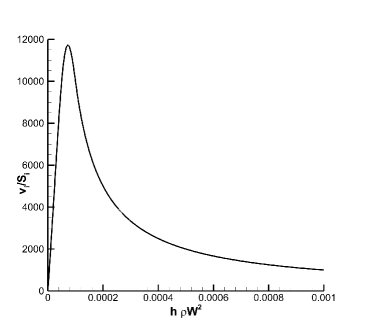
Figure 1: Plot of the velocity to momentum ratio $v_{i}/S_{i}$ when the filter function is applied. If $y=\rho hW^{2}<10^{-4}$, the filter is activated, and the velocity decreases smoothly to zero.

4 Numerical tests

In this Section we present a large set of numerical results to show all the capabilities, in terms of robustness, long-term stability and resolution, of our high order finite volume and discontinuous Galerkin schemes for the simulation of the proposed first–order hyperbolic Einstein-Euler Z4 system. If not stated otherwise, in all numerical tests we use the standard Z4 cleaning speed $e=1$ in our modified Z4 system.

We also recall that the timestep in DG schemes is restricted according to

$$\Delta t<\frac{1}{d}\frac{1}{(2N+1)}\frac{h}{|\lambda_{\max}|}\,,$$ (85)

where $h$ and $|\lambda_{\max}|$ are a characteristic mesh size and the maximum signal velocity, respectively.

4.1 Linearized gravitational wave test

As a first validation of our approach we consider a simple test, essentially one-dimensional, taken from [4] for which the metric is given as a wave perturbation of the flat Minkowski space time

$$ds^{2}=-dt^{2}+dx^{2}+(1+b)\,dy^{2}+(1-b)\,dz^{2},\quad\textnormal{with}\quad b=\epsilon\sin\left(2\pi(x-t)\right),$$ (86)

where $\epsilon=10^{-8}$ is small enough so that the model behavior is linear and the terms depending on $\epsilon^{2}$ can be neglected. According to (86) $\gamma_{xx}=1$, $\gamma_{yy}=1+b$, $\gamma_{zz}=1-b$; next, we use the harmonic gauge condition, while the gamma–driver can be turned off, i.e. $s=0$. Furthermore, the extrinsic curvature is given by $K_{ij}=\partial_{t}\gamma_{ij}/(2\alpha)$ which means that its nonzero components are only $K_{yy}=-1/2\,\partial_{t}b\text{ and }K_{zz}=1/2\,\partial_{t}b.$ The remaining non zero terms for the problem initialization are $D_{xyy}\leavevmode\nobreak\ =\leavevmode\nobreak\ 1/2\,\partial_{x}b\text{ and }D_{xzz}=-1/2\,\partial_{x}b,$ with the following setting for the other relevant parameters $\kappa_{1}=0$, $\kappa_{2}=0$ and $c=0$.

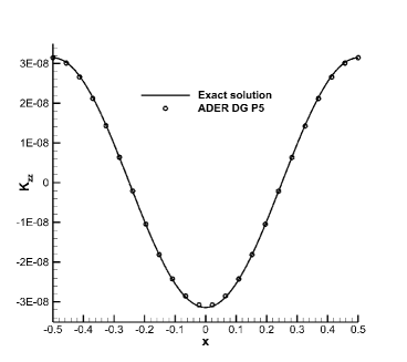
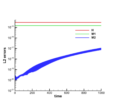
Figure 2: Linearized gravitational wave test solved with an ADER-DG scheme of order 6. Left panel: $K_{zz}$ component of the extrinsic curvature at the final time, compared to the exact solution. Right panel: Einstein constraints monitored all along the duration of the simulation.

Matter is absent in this test. To discretize the problem we consider a rectangular domain $[-0.5,0.5]\times[-0.2,0.2]$ with periodic boundary conditions, and we employ an unlimited ADER-DG scheme of order 6 on a mesh composed by $4\times 4$ elements, which corresponds to 24 degrees of freedom in each direction. We run our simulation until a final time of $t=1000$, corresponding to $1000$ crossing times. Figure 2 shows the results of the calculation. In the left panel we present the numerical solution for the $K_{zz}$ component of the extrinsic curvature, at the final time, compared with the exact one. Essentially the same perfect matching is exhibited by the other quantities. In the right panel we display instead the evolution of the Einstein constraints. As evident, in this simulation the Hamiltonian and momentum constraints are all constant up to machine precision for the entire duration of the simulation.

4.2 The gauge wave

We continue the benchmarking of our numerical scheme and of the proposed first–order hyperbolic reformulation of the $Z4$ system with the so called gauge wave test, also taken from [4]. Here, the metric is given by

$$ds^{2}=-H(x,t)\,dt^{2}+H(x,t)\,dx^{2}+dy^{2}+dz^{2},\quad\text{where}\quad H(x,t)=1-A\,\sin\left(2\pi(x-t)\right),$$ (87)

which describes a sinusoidal gauge wave of amplitude $A$ propagating along the $x$-axis. This means that the metric variables are set to $\gamma_{xx}=H$ and $\gamma_{yy}=\gamma_{zz}=1$ and the shift vector is $\beta^{i}=0$, hence the gamma–driver is switched off ($s=0$). For this test the harmonic gauge condition is used. The extrinsic curvature is again given by $K_{ij}=-\partial_{t}\gamma_{ij}/(2\alpha)$, i.e.

$$K_{yy}=K_{zz}=K_{xy}=K_{xz}=K_{yz}=0\qquad\text{and}\quad K_{xx}=-\pi A\frac{\cos\left(2\pi(x-t)\right)}{\sqrt{1-A\sin\left(2\pi(x-t)\right)}}\,.$$ (88)

All the other quantities follow accordingly, with the lapse function given by $\alpha=\sqrt{H}$. Matter is absent also in this test problem. We emphasize that the present test case, even if it can be seen as a nonlinear reparametrization of the flat Minkowski spacetime, is far from trivial: indeed, it is reported that the first and second order formulation of the classical BSSNOK system fail for this test after a rather short time, see [6, 28], and that the original version of the CCZ4 system was stable only in its damped formulation [6]. The first stable undamped simulation was reported in [59] for a first–order reformulation of the CCZ4 system. Also here for this test we use an undamped version of the PDEs with $\kappa_{1}=0$, $\kappa_{2}=0$, while we have noticed that it is necessary to set $c=1$ in the gauge condition (39) chosen with the harmonic version, i.e. $g(\alpha)=1$.

We have first run a test case with a small wave amplitude $A=0.1$ over a rectangular domain of size $[-0.5,0.5]\times[-0.02,0.02]$ with periodic boundary conditions. We have used an ADER-DG P3 numerical scheme with a uniform grid composed of $100\times 4$ elements, evolving the system until $t=1000$. Hence in the left panel of Figure 3 we show the profile of the lapse function $\alpha$ as a representative quantity, showing a perfect matching with the exact solution at the final time. In the right panel, on the other hand, we monitor as usual the Einstein constraints, which manifest a moderate linear growth all along the evolution.

Then, we have considered a large amplitude perturbation with $A=0.9$, to the extent of performing a numerical convergence analysis of our scheme. The computational domain in this case is given by $[-0.5,0.5]\times[-0.05,0.05]$. The results, extracted from data at time $t=10$, are reported in Table 1 and confirm that the scheme reaches the nominal order of convergence.

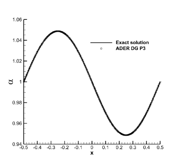
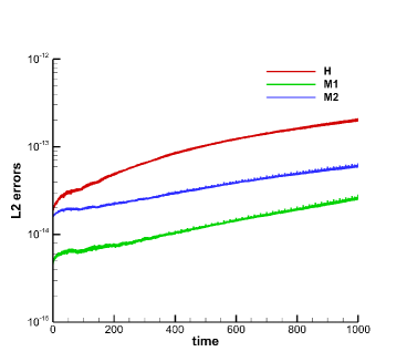
Figure 3: Solution of the gauge wave test at $t=1000$ with $A=0.1$ using an ADER DG scheme of order 4. Left panel: profile of the lapse $\alpha$ compared to the exact solution. Right panel: Evolution of the Einstein constraints.

Gauge wave — ADER-DG-$\mathbb{P}_{N}$
	$N_{x}\times N_{y}$	$L^{1}$ error	$L^{2}$ error	$L^{\infty}$ error	$L^{1}$ order	$L^{2}$ order	$L^{\infty}$ order	Theor.
DG-$\mathbb{P}_{2}$	$40\times 4$	1.2838E-03	4.8661E-03	2.5095E-02	—	—	—	3
	$60\times 6$	2.6423E-04	9.8619E-04	4.9053E-03	3.90	3.94	4.03
	$80\times 8$	8.2440E-05	3.0322E-04	1.5083E-03	4.05	4.10	4.10
	$100\times 10$	3.3280E-05	1.2108E-04	6.0413E-04	4.07	4.11	4.10
DG-$\mathbb{P}_{3}$	$40\times 4$	5.3398E-05	2.0348E-04	1.0660E-03	—	—	—	4
	$60\times 6$	1.2460E-05	4.7006E-05	2.3760E-04	3.59	3.61	3.70
	$80\times 8$	4.1667E-06	1.5621E-05	7.7947E-05	3.81	3.83	3.87
	$100\times 10$	1.7520E-06	6.5436E-06	3.2420E-05	3.88	3.90	3.93
DG-$\mathbb{P}_{4}$	$40\times 4$	1.8236E-06	6.7109E-06	3.3969E-05	—	—	—	5
	$60\times 6$	1.6400E-07	5.8994E-07	2.8784E-06	5.94	6.00	6.09
	$80\times 8$	2.9500E-08	1.0461E-07	4.9922E-07	5.96	6.01	6.09
	$100\times 10$	7.7948E-09	2.7398E-08	1.2988E-07	5.96	6.00	6.03
DG-$\mathbb{P}_{5}$	$40\times 4$	5.5287E-08	2.0571E-07	1.1845E-06	—	—	—	6
	$60\times 6$	6.2100E-09	2.2674E-08	1.1696E-07	5.39	5.44	5.71
	$80\times 8$	1.2027E-09	4.3669E-09	2.1883E-08	5.71	5.73	5.83
	$100\times 10$	3.3009E-10	1.1974E-09	5.9321E-09	5.79	5.80	5.85
DG-$\mathbb{P}_{6}$	$40\times 4$	2.8610E-09	1.0215E-08	5.2758E-08	—	—	—	7
	$50\times 5$	5.0341E-10	1.7825E-09	8.9322E-09	7.79	7.82	7.96
	$60\times 6$	1.2258E-10	4.3434E-10	2.5857E-09	7.75	7.74	6.80
	$70\times 7$	3.8840E-11	1.3929E-10	1.0035E-09	7.46	7.38	6.14

Table 1: Numerical convergence results for the gauge wave test at $t=10$ with a wave amplitude $A=0.9$. In the table we report the $L_{1}$, $L_{2}$, $L_{\infty}$ error norms and the corresponding numerical order of convergence for the lapse $\alpha$.

4.3 The robust stability test

Another important validation for any numerical GR code is represented by the so–called robust stability test in a flat Minkowski spacetime without matter, already treated by [4, 59]. It consists of a random perturbation with amplitude $\pm 10^{-7}/\varrho^{2}$ which is applied to all quantities of the PDE system in a flat Minkowski spacetime. The amplitude of the perturbation that we have chosen is three orders of magnitude higher than that reported in [4]. The computational domain is given by the square $[-0.5;0.5]\times[-0.5;0.5]$, for which we have considered four simulations with an unlimited ADER-DG $P_{3}$ scheme on a sequence of refined meshes formed by $10\varrho\times 10\varrho$ elements, where $\varrho\in\left\{1,2,4,8\right\}$ is the refinement factor.

This is also a test for the gamma–driver shift condition, which, in principle, would not be necessary for this kind of problem but is nevertheless activated to solve the PDE system in its full generality. The other relevant parameters have been chosen as $\kappa_{1}=0$, $\kappa_{2}=0$, $c=0$, $\mu=0.2$, $\eta=0$, see (41) and (43). Fig. 4 shows the results of our calculations, where we have reported the evolution of the four Einstein constraints for a sample of progressively refined meshes. The unit of time is again the travel time taken by light to cover the edge of the square domain.

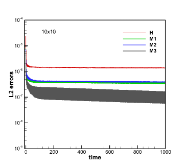
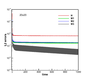
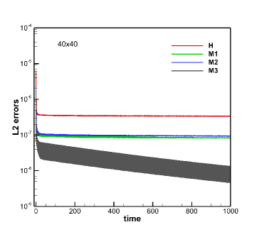
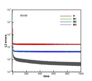
Figure 4: Robust stability test case with a random initial perturbation of amplitude $10^{-7}/\rho^{2}$ in all quantities on a sequence of successively refined meshes on the unit square in 2D. The gamma–driver shift condition, $1+\log$ slicing and ADER-DG $P_{3}$ scheme have been used. Top left: $10\times 10$ elements, corresponding to $40\times 40$ degrees of freedom ($\varrho=1$). Top right: $20\times 20$ elements, corresponding to $80\times 80$ degrees of freedom ($\varrho=2$). Bottom left: $40\times 40$ elements, corresponding to $160\times 160$ degrees of freedom ($\varrho=4$). Bottom right: $80\times 80$ elements, corresponding to $320\times 320$ degrees of freedom ($\varrho=8$).

4.4 Spherical Michel accretion

As a further test, we have evolved the transonic spherical accretion solution of matter onto a Schwarzschild black hole obtained by [109] (see also [131] for a modern presentation). We recall that this is not a solution of the full Einstein–Euler equations, but rather just of the Euler equations in the stationary background spacetime of a non–rotating black hole. However, if the whole mass accretion rate is small enough, we can neglect the increase of the black hole mass that would in principle be produced by the accreated matter. Under such circumstances we can consistently evolve the Euler equations while freezing the evolution of the metric, i.e. assuming what is referred to as the Cowling approximation [46].

The numerical details for obtaining the initial conditions can be found in [10]. We have performed this simulation in spheroidal Kerr–Schild coordinates (see case 1. of Sect. 3.3) over a two dimensional computational domain given by $(r,\theta)\in[0.5;10]\times[0+\epsilon;\pi-\epsilon]$, with $\epsilon=0.005$ and covered by a $50\times 32$ uniform grid. The critical radius, where the flow becomes supersonic, is $r_{c}=5$ (inside the computational domain). We choose the critical density (density at the critical radius) $\rho_{c}=1.006\times 10^{-7}$ such that the mass accretion rate (computed as $4\pi r_{c}^{2}\rho_{c}u_{c}^{r}$) is $-1.0\times 10^{-5}$, meaning that the total mass accreated onto the black hole from $t=0$ to $t=1000\,M$ is just $1/100$ of the total mass $M$ of the central black hole, thus justifying the physical assumption of a stationary spacetime. We stress that, with these parameters characterized by very low rest mass densities, the test becomes extremely challenging from the numerical point of view, in spite of the solution being smooth and regular.

The equation of state is that of an ideal gas with adiabatic index $\gamma=5/3$.

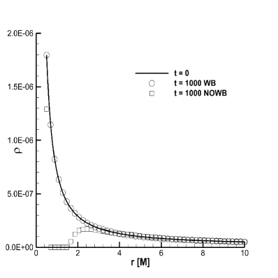
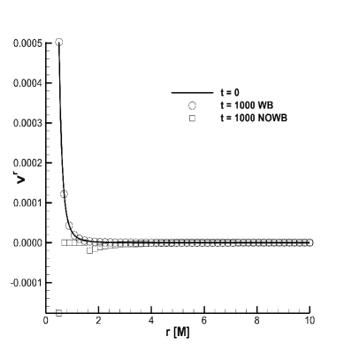
Figure 5: Solution of the spherical accretion of matter onto a non-rotating black hole. The final rest mass density (left panel) and the radial velocity (right panel) at time $t=1000\,M$ are compared to their initial profiles.

At time $t=0$, the rest mass density of the exact solution is perturbed by a Gaussian profile peaked at the critical radius, with an amplitude given by $\delta\rho=10^{-3}\rho_{c}$. We have solved this test by considering only the hydrodynamic section of the system (32)–(2.3), thus adopting the Cowling approximation. The numerical scheme is a pure DG scheme at fourth order of accuracy ($N=3$), while the other relevant parameters have been chosen as $\kappa_{1}=0.01$, $\kappa_{2}=0$, $c=0$, with no gamma–driver. We have performed two simulations to the final time $t=1000\,M$, the first one with the new well-balancing technique described in Sect. 3, and a second one without it, obtaining rather different results. Figure 5 reports the one dimensional profiles of the solution for the rest mass density and for the radial velocity $v^{r}$ at the final time compared to the exact solution. If no well-balancing is adopted, the solution quickly deteriorates, amounting to a sequence of failures in the recovering of the primitive variables, as can be seen by the zero density values reported in the left panel of Figure 5. If the well-balancing is used instead, the exact solution is recovered and stationarity is preserved. We recall that the positive values of the the radial velocity, which are somewhat counter intuitive given that matter is falling into the black hole with increasing velocity, are a spurious effect of the Kerr–Schild coordinates, which generate a positive radial shift.

We also stress that in these regimes of low density matter, using the filter described in Sect. 3.4 is absolutely crucial, and the simulation encounters a sequence of catastrophic failures before $t\sim 5M$ if no filter is adopted, irrespective of the well-balancing property being activated, or not.

4.5 Single stationary black holes in two and three space dimensions

The Schwarzschild solution, historically the first exact solution that was found for the Einstein field equations, describes the spacetime around a non–rotating black hole and it represents a static solution of the Einstein field equations. A generalization to rotating black holes is the stationary Kerr solution. For all simulations reported in this section, the mass of the black hole is $M=1\,M_{\odot}$. In all tests presented here, matter is absent.

Non-rotating black hole in 2D

In our first simulation we solve the Z4 equations for a Schwarzschild black hole ($a=0$) in spherical Kerr–Schild coordinates, see Sect. 3.3. The two–dimensional computational domain in the $r-\theta$ plane is chosen as $\Omega=[0.5,6]\times[\delta,\pi-\delta]$, with $\delta=0.1415926535$. The domain $\Omega$ is discretized with $80\times 40$ elements. On all boundaries we prescribe the initial condition as Dirichlet boundary condition for all state variables. We use the fourth order version ($N=3$) of our new exactly well-balanced ADER-DG scheme based on the HLL Riemann solver and without any subcell FV limiter. Concerning the Z4 system we use the 1+log gauge condition and set $c=0$, $\kappa_{1}=1.0$, $\kappa_{2}=1.0$ and $s=0$, i.e. the shift is not evolved in time. In order to study the behaviour of the new well-balanced scheme in the presence of a small perturbation, the initial condition for the cleaning variable $\Theta$ is chosen as

$$\Theta(0,\mathbf{x})=A_{0}\exp\left(-\frac{1}{2}\frac{(X-4)^{2}+(Y-0)^{2}}{\sigma^{2}}\right)\,,$$ (89)

with $(x_{1},x_{2})=(r,\theta)$, $A_{0}=10^{-3}$, $\sigma=0.2$, $X=r\sin\theta$ and $Y=r\cos\theta$. We expect that during the simulation the perturbation leaves the computational domain and that for large enough times the solution returns back to the exact stationary equilibrium solution. The computational results obtained for this simulation are shown in Figure 6. In the top left panel we plot the $L^{2}$ norms of the constraint violations $H(t)-H(0)$ and $M_{i}(t)-M_{i}(0)$ for the Hamiltonian and the momentum constraints. As expected, the initial perturbation of the order $10^{-3}$ decays exponentially in time and the solution returns back to the exact equilibrium. To the best knowledge of the authors, this is the first long-time simulation ever carried out for the Einstein field equations using a high order exactly well-balanced discontinuous Galerkin finite element scheme and where, after an initial perturbation, the discrete solution returns back to the exact steady equilibrium solution. In the remaining panels of Figure 6 we show one dimensional profiles obtained from cuts along the equatorial plane, for various representative quantities like $\alpha$, $\gamma_{11}$, $K_{11}$. As apparent from the figure, perfect agreement with the exact stationary solution is obtained at the final time $t=1000\,M$.

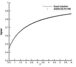
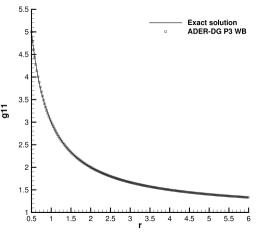
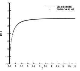
Figure 6: 2D simulation of an initially perturbed Schwarzschild black hole ($a=0$) in the 2D plane $r-\theta$ using spherical Kerr-Schild coordinates. Top left: time series of the constraint violations until time $t=1000\,M$. It is clearly visible that the initial perturbation decays exponentially in time and that the numerical solution returns to the stationary equilibrium. From top right to bottom right: 1D cuts along the radial direction at $\theta=\pi/2$ for the lapse $\alpha$, the metric tensor component $\gamma_{11}$ and the extrinsic curvature component $K_{11}$ at time $t=1000\,M$ and comparison with the exact solution.

Numerical study of the well-balancing property

We now repeat the previous test of the non-rotating black hole in 2D until $t=0.1$ using a fourth order ADER-DG scheme ($N=3$) on $40\times 20$ elements and employing three different machine precisions, namely single, double and quadruple precision. We set the perturbation amplitude $A_{0}$ so that it corresponds to the respective machine precision. The values of $A_{0}$ as well as the obtained $L^{\infty}$ error norms are reported in Table 2 at time $t=0.1$ for several components of the Z4 system and for all chosen machine precisions. The computational results clearly show that the errors remain of the order of machine precision, hence the new numerical method proposed in this paper is well-balanced also in its practical implementation, as expected.

Table 2: Numerical well-balancing test with a fourth order ADER-DG scheme using single, double and quadruple precision. $L^{\infty}$ error norms for several quantities of the Z4 system at time $t=0.1$.

Quantity	single precision, $A_{0}=10^{-8}$	double precision, $A_{0}=10^{-16}$	quadruple precision, $A_{0}=10^{-28}$
$\alpha$	7.4505806E-06	3.2196468E-015	4.7282543E-030
$\gamma_{11}$	7.8201294E-05	3.3306691E-014	2.2768344E-030
$K_{11}$	8.1777573E-05	3.2862602E-014	2.8324170E-029
$K_{12}$	2.7160518E-06	1.9922607E-015	1.5911163E-029
$\Theta$	2.6383780E-06	1.6878889E-015	3.4825676E-029
$Z_{1}$	9.8760290E-07	1.3437779E-015	2.3198075E-029
$A_{1}$	9.4473362E-06	4.8849813E-015	1.8991764E-029
$D_{111}$	3.3855438E-05	1.3766766E-014	4.5212168E-030

Non-rotating black hole in 3D

We have then evolved the same stationary Schwarzschild black hole ($a=0$) in three space dimensions by choosing the 3D Cartesian Kerr–Schild coordinates already discussed in Sect. 3.3. The computational domain is the box $[-5;5]\times[-5;5]\times[-5;5]$, from which we have excised a cubic box with an edge of length $1.0$ centered on the physical singularity at $r=0$. The resolution is $20^{3}$, and similarly to the two-dimensional case, a perturbation is introduced in the variable $\Theta$. Again with a fourth order well-balanced ADER-DG scheme, we obtain the results that are shown in Fig. 7. The constraint violations decay back to the equilibrium at time $t\approx 400\,M$, after which the solution is perfectly stable around machine precision. For this simulation, the 1D cuts are extracted along the $z$ axis.

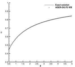
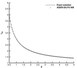
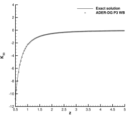
Figure 7: 3D simulation of an initially perturbed Schwarzschild black hole (spin $a=0$) in 3D Cartesian Kerr-Schild coordinates using a fourth order well-balanced ADER-DG scheme. Top left: time series of the constraint violations until time $t=1000\,M$. It is clearly visible that the initial perturbation decays exponentially in time and that the numerical solution returns to the stationary equilibrium. From top right to bottom right: 1D cuts along the z axis ($x=y=0$) for the lapse $\alpha$, the metric tensor component $\gamma_{11}$ and the extrinsic curvature component $K_{11}$ at time $t=1000\,M$ and comparison with the exact solution.

Rotating black hole in 3D

Finally, in addition to the previous Schwarzschild black holes with $a=0$, we have also evolved two Kerr black holes in three space dimensions, one with spin $a=0.5$ and the other one with spin $a=0.99$. The computational domain is the box $[-5;5]\times[-5;5]\times[-5;5]$, with the same resolution as for the Schwarzschild case, namely $20^{3}$. A major difference is given by the fact that the excision box must enclose the ring singularity on the $z=0$ plane [47], which has an external radius $r_{\rm{ring}}=a$. Hence, the excision box is effectively a parallelepiped with edges $2\times 2\times 1$, and $3.2\times 3.2\times 1$, for the two black holes with spin $a=0.5$ and $a=0.99$, respectively. Keeping the same strategy of perturbing the initial configuration, we obtain results that are shown in Fig. 8 and Fig. 9, and confirming the turning back of the solution to the exact equilibrium. Fig. 10, on the other hand, shows the contour surfaces of a few representative quantities where the Schwarzschild ($a=0$) and the Kerr ($a=0.99$) black holes are compared.

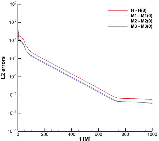
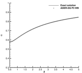
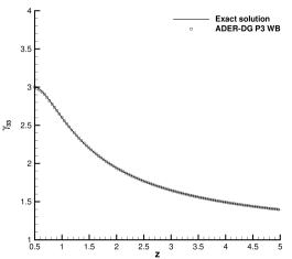
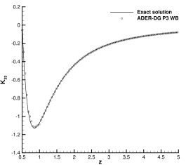
Figure 8: 3D simulation of an initially perturbed Kerr black hole (spin $a=0.5$) in 3D Cartesian Kerr-Schild coordinates using a fourth order well-balanced ADER-DG scheme. Top left: time series of the constraint violations until time $t=1000\,M$. It is clearly visible that the initial perturbation decays exponentially in time and that the numerical solution returns to the stationary equilibrium. From top right to bottom right: 1D cuts along the z axis ($x=y=0$) for the lapse $\alpha$, the metric tensor component $\gamma_{33}$ and the extrinsic curvature component $K_{33}$ at time $t=1000\,M$ and comparison with the exact solution.

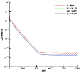
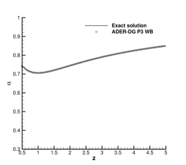
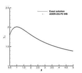
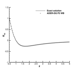
Figure 9: 3D simulation of an initially perturbed Kerr black hole (spin $a=0.99$) in 3D Cartesian Kerr-Schild coordinates using a fourth order well-balanced ADER-DG scheme. Top left: time series of the constraint violations until time $t=1000\,M$. It is clearly visible that the initial perturbation decays exponentially in time and that the numerical solution returns to the stationary equilibrium. From top right to bottom right: 1D cuts along the z axis ($x=y=0$) for the lapse $\alpha$, the metric tensor component $\gamma_{33}$ and the extrinsic curvature component $K_{33}$ at time $t=1000\,M$ and comparison with the exact solution.

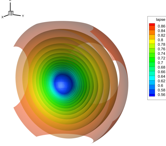
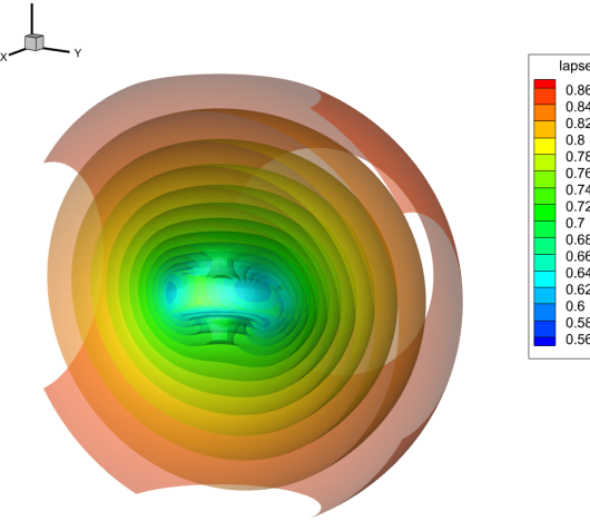
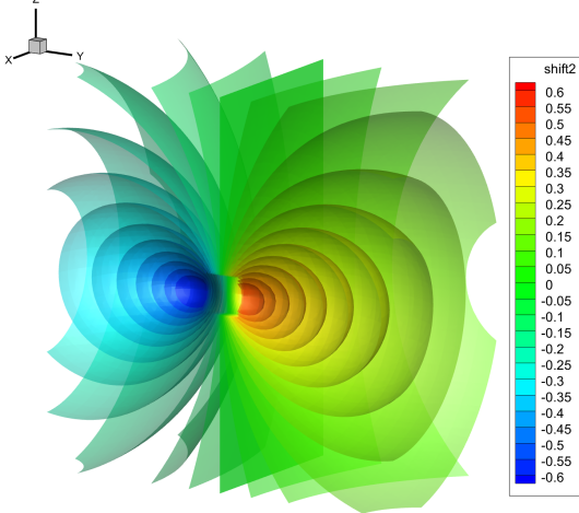
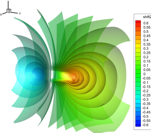
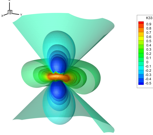
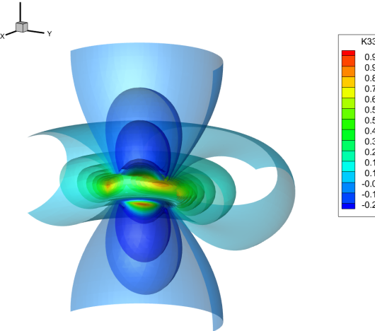
Figure 10: Contour surfaces of initially perturbed black hole spacetimes in 3D Cartesian Kerr-Schild coordinates at $t=1000\,M$ using a fourth order well-balanced ADER-DG scheme. Left: Schwarzschild black hole ($a=0$). Right: Kerr black hole ($a=0.99$). From top to bottom: lapse $\alpha$, shift $\beta_{2}$ and extrinsic curvature component $K_{33}$.

4.6 Non–rotating neutron star in equilibrium

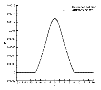
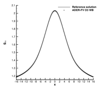
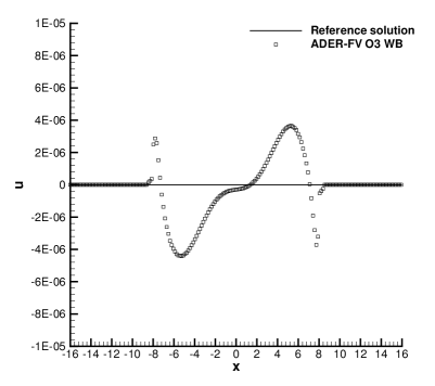
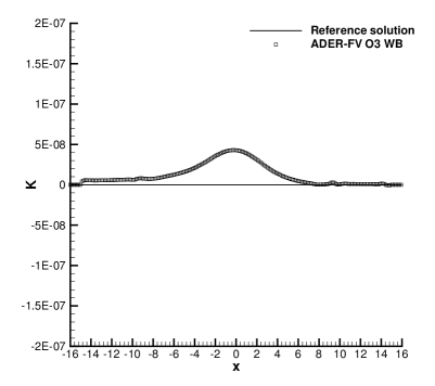
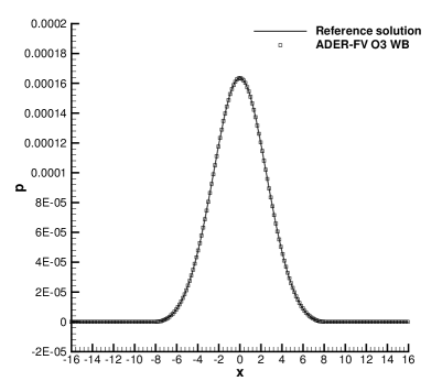
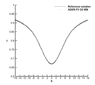
Figure 11: 1D cuts of some hydrodynamic and metric quantities of the TOV star obtained with the new well-balanced third order ADER-FV scheme at the final time $t=1000\,M$.

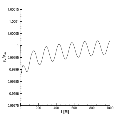
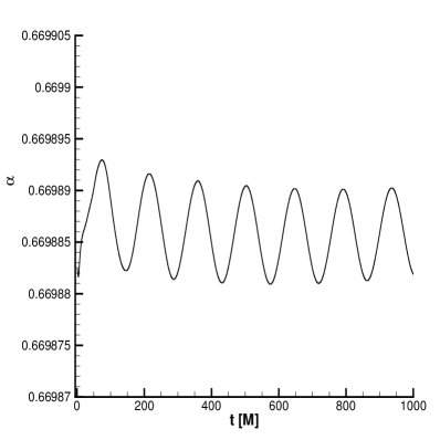
Figure 12: Time evolution of the central mass density (left panel) and of the central lapse (right panel) for the 3D TOV star.

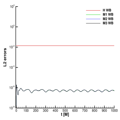
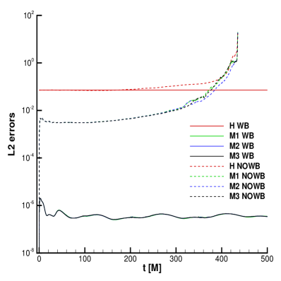
Figure 13: Time evolution of the constraint violations for the stable 3D TOV star. Left panel: well-balanced third order ADER-FV scheme. Right panel: well-balanced third order ADER-DG scheme vs. not well-balanced third order ADER-DG scheme ($N=2$).

A crucial test for numerical relativity, where both the Einstein and the relativistic Euler equations must be accounted for, is represented by the time evolution of an equilibrium neutron star. In the non–rotating case, this amounts to solving the so called Tolman–Oppenheimer–Volkoff (TOV) system, which we report here for completeness [142, 119, 131]

$$\frac{dm}{dr} =4\pi r^{2}e\,,$$ (90)

$$\frac{dp}{dr} =-\frac{(e+p)(m+4\pi r^{3}p)}{r(r-2m)}\,,$$ (91)

$$\frac{d\phi}{dr} =-\frac{1}{e+p}\frac{dp}{dr}\,,$$ (92)

where $m(r)$ is the mass enclosed within the radius $r$, $\phi$ is the unknown metric function in the line element (69), while $e^{-2\psi}=1-\frac{2m}{r}$. The equation of state adopted is that of a polytropic gas, namely $p=K\,\rho^{\gamma}$.

The TOV system (90)–(92) constitutes a set of three ODEs, which we have solved using a tenth order accurate discontinuous Galerkin scheme, see [55]. For high order ADER-DG schemes, in fact, simple initial data computed via Runge-Kutta ODE integrators are not accurate enough. We have adopted a stable model with parameters which have by now become canonical in numerical relativity [74], namely a central rest mass density $\rho_{c}=1.28\times 10^{-3}$, $K=100$ and $\gamma=2$. Having done that, the numerical integration of (90)–(92) provides all the radial profiles as well as the remaining physical characteristics of the star, i.e. a total mass $M=1.4\,M_{\odot}$ and a radius $R=9.585\,M_{\odot}=14.15\,km$. When performing the coordinate transformation

$$\frac{d\bar{r}}{\bar{r}}=\left(1-\frac{2m}{r}\right)^{-1/2}\frac{dr}{r},$$ (93)

see [30], then the spatial part of the metric (69) becomes conformally flat, namely

$$ds^{2}=-e^{2\phi}dt^{2}+e^{2\bar{\psi}}(d\bar{r}^{2}+\bar{r}^{2}d\theta^{2}+\bar{r}^{2}\sin^{2}\theta d\phi^{2})=-e^{2\phi}dt^{2}+e^{2\bar{\psi}}(d\bar{x}^{2}+d\bar{y}^{2}+d\bar{z}^{2})\,,$$ (94)

thus generating a spatial metric that is just $\gamma_{ij}=(r/\bar{r})^{2}\eta_{ij}$. In the space outside the star, due to Birkoff's theorem, the spacetime is that of a Schwarzschild solution produced by a mass $M$, i.e.

$$e^{2\phi}=1-\frac{2M}{r},\hskip 28.45274pt\bar{r}=\frac{1}{2}\left(\sqrt{r^{2}-2Mr}+r-M\right),$$ (95)

while all the hydrodynamic variables collapse to zero. The initial equilibrium model is perturbed in the energy density $h$ by a small amplitude Gaussian profile, and then the full Einstein–Euler system is evolved until $t=1000\,M$. We stress that, thanks to our new conversion from the conservative to the primitive variables (see Sect. 3.4), there is no need to insert a low density atmosphere in the exterior of the neutron star. For this test the fluid pressure was initially perturbed by adding a small fluctuation $p^{\prime}=p_{0}\exp\left(-\frac{1}{2}\frac{\mathbf{x}^{2}}{\sigma^{2}}\right)$ to the pressure obtained from the TOV solution, with amplitude $p_{0}=10^{-7}$ and halfwidth $\sigma=0.2$.

To obtain better results, and only for this test, we had to resort to a well-balanced third order ADER-FV scheme [63], which became necessary for its increased robustness with respect to ADER-DG, especially at the surface of the star. Figure 11 shows the results of our computations, by reporting the 1D-cuts of a few representative quantities at the final time, compared to the reference equilibrium solution. A perfect matching is obtained, apart for very small deviations in the profiles of the velocity (along $x$) and in the trace of the extrinsic curvature $K$. To the best of our knowledge, this is the first time that a numerical relativity code can evolve a TOV star in a (matter) vacuum atmosphere with $\rho=p=0$.

In addition, in Fig. 12 we report the time evolution of the central rest–mass density (left panel, normalized to its initial value) and of the central lapse (right panel). We just mention briefly that from this oscillating behavior it is possible to extract the normal modes of oscillation of the neutron star, comparing them with those obtained through a perturbative analysis and inferring fundamental aspects of neutron star physics [75]. As we are not interested to enter such details in this work, we postpone further analysis to future investigations.

Finally, Fig. 13 shows the behaviour of the Einstein constraints during the evolution. The left panel refers to the same simulation reported in Fig. 11, and it shows that the $L^{2}$ norm of the Einstein constraints remains low and stationary all along the evolution. The right panel refers instead to a second simulation with the third–order ADER-DG scheme. In this case we have compared the well-balanced (WB) algorithm with the not well-balanced (NOWB) one. The difference is remarkable, since in the not well-balanced evolution (NOWB) the Einstein constraints start increasing around $t\sim 300$, entering an exponential grow which eventually makes the code crash.

4.7 Two puncture black holes

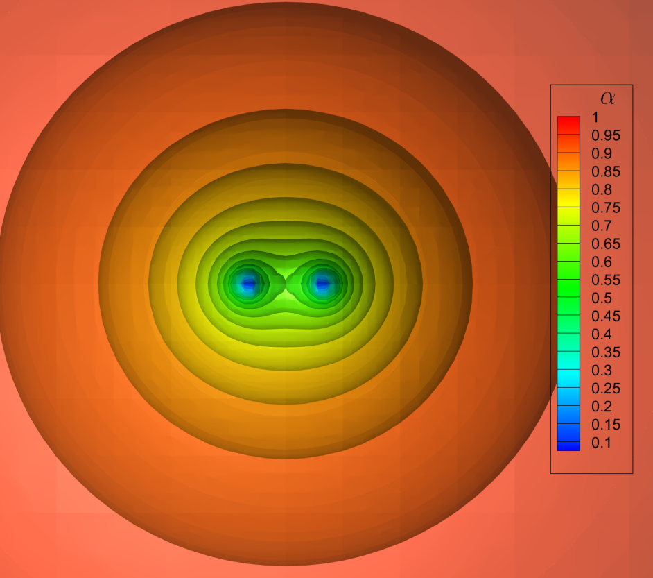
$t=0$

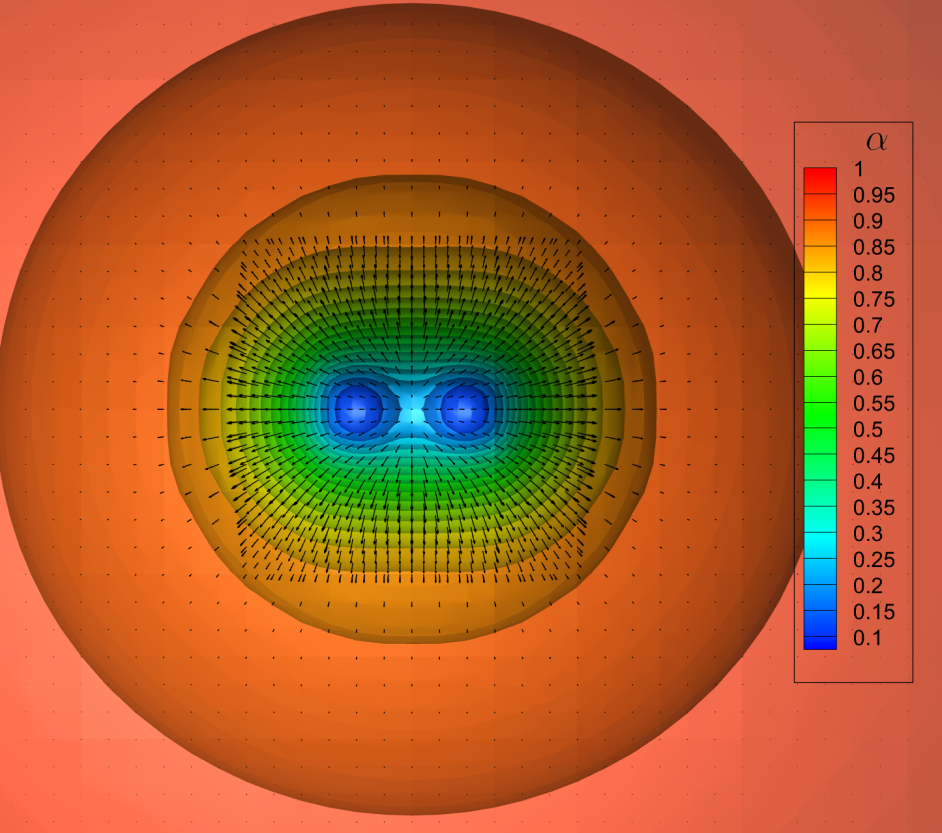
$t=5$

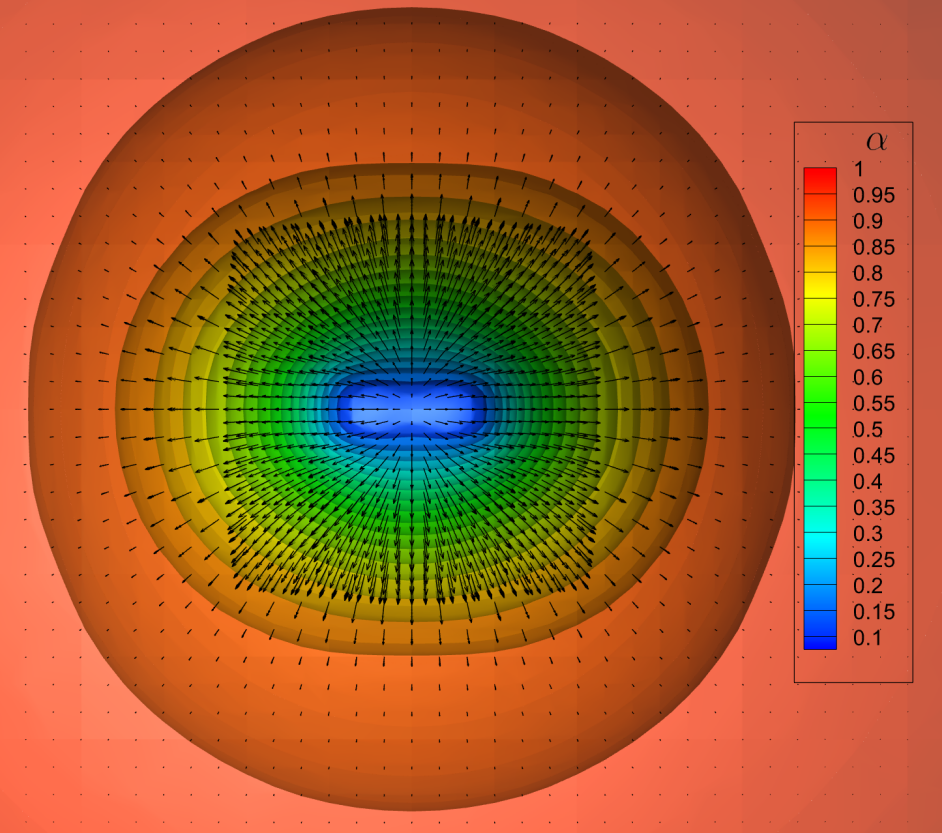
$t=7$

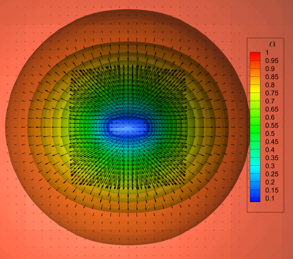
$t=8$

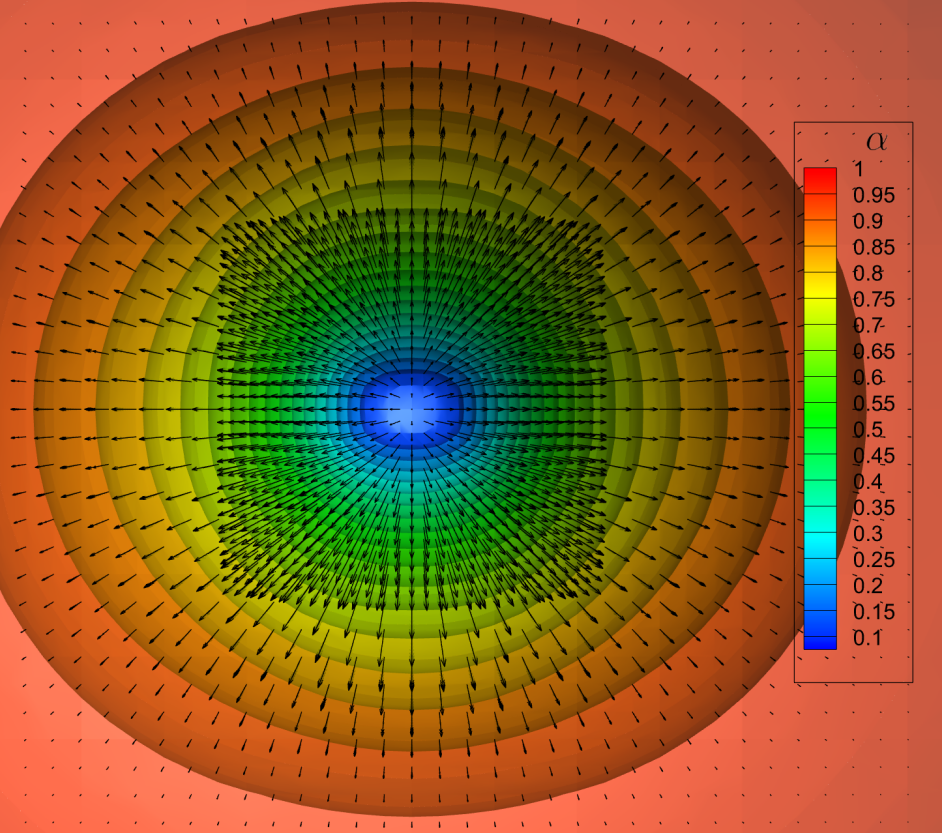
$t=10$

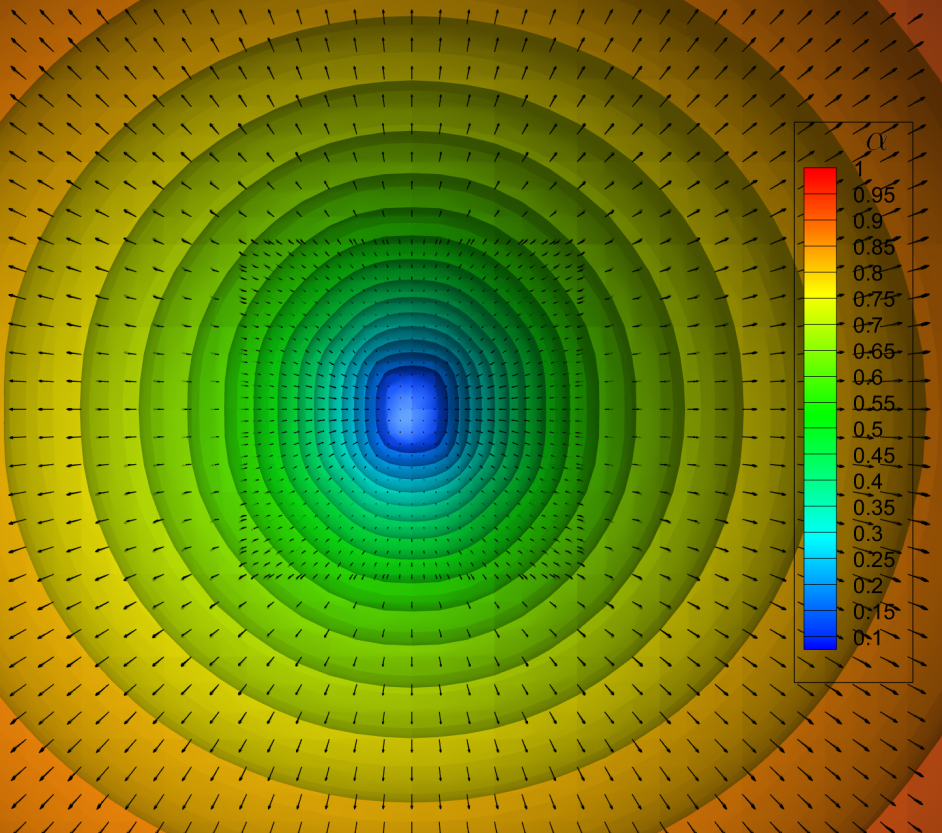
$t=20$

Figure 14: Contour surfaces of the lapse for the two punctures black holes. The solution is reported at six different times: $t=0,5,7,8,10,20\,M$.

Figure 15: Time evolution of the constraint violations for two punctures black holes.

As a last test we have analyzed the head-on collision of two nonrotating black holes, which are modeled as two moving punctures. The initial conditions can be obtained by the TwoPunctures initial data code [9], and are prescribed as follows:

• equal black hole masses, $M=1$, with no spin;

• initial positions given by $\bm{x}^{-}=(-1,0,0)$ and $\bm{x}^{+}=(+1,0,0)$;

• zero linear momenta;

• zero initial extrinsic curvature.

We have performed this test to the purpose of showing the ability of the DG scheme based on our improved Z4 implementation of the Einstein equations to solve moving punctures, irrespective of the possibility of extracting gravitational waves, which will be the subject of a future research. The three-dimensional computational domain is given by $\Omega=[-60;60]^{3}$ and flat Minkowski spacetime is imposed as boundary condition everywhere. We use adaptive mesh refinement (AMR) with time accurate local time stepping [63] and one level of refinement with refinement factor $\varrho=3$ inside the box $[-10,10]^{3}$. The subcell finite volume limiter is always activated within the box $[-3,3]^{3}$. The numerical relevant parameters are set as $\kappa_{1}=0.2$, $\kappa_{2}=0.2$, $c=0$, $\mu=0.0$.

For this test, the activation of the gamma–driver is mandatory. In order for the evolution to proceed successfully, we have found that it is necessary to perform the following actions: in the inner region the lapse $\alpha$ is flattened as

$$\alpha=\frac{\alpha r^{6}+\epsilon\alpha_{min}}{r^{6}+\epsilon}\,,$$ (96)

where $\alpha_{min}=0.01$, $\epsilon=10^{-4}$, in such a way that the spacetime evolution is effectively frozen. Simultaneously, all the metric terms are filtered as

$$f = \operatorname{erf}\left(\frac{\gamma_{max}}{\gamma_{ij}}\left[1+\left(\frac{r}{0.4}\right)^{4}\right]\right),$$ (97)

$$\gamma_{ij} = \gamma_{max}(1-f)+\gamma_{ij}f\,,$$ (98)

so as to avoid metric spikes, but rather reaching a smooth maximum value at $\gamma_{max}\sim 25$. In addition, since there is not an exact solution for this test, the well-balancing property is switched off completely.

In Figure 14 we present the contour iso-surfaces of the lapse at different times, showing the merger process of the two black holes. In Figure 15 the time evolution of the Hamiltonian and momentum constraints are reported, showing a stable evolution of the system until the end of the merger process. To the very best knowledge of the authors, this is the very first stable 3D simulation of a head-on collision of two puncture black holes carried out with a high order DG scheme applied to the first order reformulation of the Z4 system of the Einstein field equation.

5 Conclusions

In this paper we have investigated the first–order version of the Z4 formulation of the Einstein–Euler equations, originally proposed by [21, 22], via a new well-balanced discontinuous Galerkin scheme for non conservative systems. We have shown substantial advantages with respect to its analogous first–order CCZ4 version, already discussed in [59]. Along with an obvious simpler form of the equations, when compared to CCZ4, in the Z4 system the $Z^{\mu}$ four vector is an evolved quantity, allowing for a direct monitoring of the Einstein constraints violations. Strong hyperbolicity has been verified by computing the full set of eigenvectors for a general metric in case of frozen shift. The new high order well-balanced ADER-DG scheme for conservative and non-conservative systems relies on the framework of path-conservative schemes. The choice of the path is irrelevant in the case of the Einstein field equations, since the non-conservative part of the system concerns only the metric, which cannot develop discontinuities as all associated characteristic fields are linearly degenerate. We have verified the nominal order of convergence of our new scheme up to seventh order in space and time. Two additional and fundamental features make the new numerical scheme particularly robust and attractive:

1. The overall scheme is well-balanced, in the sense that it can preserve stationary equilibrium solutions exactly up to machine precision. This has been obtained in a pragmatic but very effective way by subtracting the discretized equilibrium solution from the evolved one during the simulation. For highly dynamical systems, on the other hand, the well-balancing property is not useful and hence not adopted.

2. The conversion from the conservative to the primitive variables, which has been plaguing relativistic hydrodynamic codes for so long, has been made substantially more robust by the introduction of a special filter function, which avoids division by zero and thus the divergence of the velocity in regimes of very low rest mass densities. To the best of our knowledge, this is the very first time that compact objects like neutron star can be simulated by setting $\rho=0$ outside the object, instead of requiring a numerical atmosphere.

After these improvements, we have been able to reproduce all the standard tests of numerical relativity with unprecedented accuracy in the computation of stationary solutions. In particular, and to the best of our knowledge, this is the first time that a stationary black hole (including an extreme Kerr one with $a=0.99$) has been evolved with a high order DG scheme in three space dimensions within the 3+1 formalism up to $t=1000M$, and with no limitation to proceed even further.

Second, our new filter in the conversion from the conserved to the primitive variables allowed us to evolve a TOV star in true vacuum, namely with $p=\rho=0$ outside the star. This new feature is likely to play a major role in future applications of high energy astrophysics where very low density regions are involved.

Finally, at the level of a proof of concept calculation and with no intention yet to compute the gravitational wave emission from a binary system, we have obtained first encouraging preliminary results concerning the head–on collision of two equal masses black holes. This demonstrates the possibility to account for a physical problem that was previously considered off–limits for the original Z4 formulation.

Future work will concern the application of the new numerical scheme to the simulation of the inspiral and merger of binary black holes and binary neutron star systems with the calculation of the related gravitational waves.

6 Acknowledgments

This work was financially supported by the Italian Ministry of Education, University and Research (MIUR) in the framework of the PRIN 2022 project High order structure-preserving semi-implicit schemes for hyperbolic equations and via the Departments of Excellence Initiative 2018–2027 attributed to DICAM of the University of Trento (grant L. 232/2016). M.D. and I.P. are members of the INdAM GNCS group in Italy.

E. Gaburro is member of the CARDAMOM team at the Inria center of the University of Bordeaux and gratefully acknowledges the support received from the European Union’s Horizon 2020 Research and Innovation Programme under the Marie Skłodowska-Curie Individual Fellowship SuPerMan, grant agreement No. 101025563.

We would like to thank Luciano Rezzolla and Konrad Topolski for rather valuable discussions.

Appendix A The eigenstructure of the first–order Z4 system

We stress that the Euler and the Einstein sector of the full PDE given by (32)–(2.3) are coupled only through the source terms, since all the metric derivatives arising in the matrix $\partial{\bf F}(\mathbf{Q})/\partial\mathbf{Q}$, and corresponding to the Euler block, have been moved to the source terms on the right hand side as auxiliary variables. Hence, with no loss of generality, we can analyze the eigenstructure of the Einstein–Euler system by focusing on the Einstein block, more specifically by setting to zero all the hydrodynamic variables $(D,S_{1},S_{2},S_{3},E)$, whose eigenvectors are well known. In addition, assuming the 1+log gauge condition with zero shift ($\beta^{i}=0$, $s=0$), excluding the passive quantity $K_{0}$ from the analysis, and using $c=0$, the remaining 55 variables for the state vector $\mathbf{Q}$ relative to the matter and spacetime evolution are given by

$${\bm{Q}}^{T} = \Big{(}D,S_{1},S_{2},S_{3},E,\ln{\alpha},\beta^{1},\beta^{2},\beta^{3},\gamma_{11},\gamma_{12},\gamma_{13},\gamma_{22},\gamma_{23},\gamma_{33},K_{11},K_{12},K_{13},K_{22},K_{23},K_{33},\Theta,Z_{1},Z_{2},Z_{3},$$ (99)

$$A_{1},A_{2},A_{3},B^{\,\,1}_{1},B^{\,\,1}_{2},B^{\,\,1}_{3},B^{\,\,2}_{1},B^{\,\,2}_{2},B^{\,\,2}_{3},B^{\,\,3}_{1},B^{\,\,3}_{2},B^{\,\,3}_{3},D_{111},D_{112},D_{113},D_{122},D_{123},D_{133},D_{211},D_{212},D_{213},$$

$$D_{222},D_{223},D_{233},D_{311},D_{312},D_{313},D_{322},D_{323},D_{333},\Big{)}\,.$$

Under such circumstances, the eigenvalues are given by

$$\begin{array}[]{llll}\lambda_{1}&=&\sqrt{\gamma^{11}}\alpha\,e&\textrm{(multiplicity 1)}\,,\\ \lambda_{2}&=&-\sqrt{\gamma^{11}}\alpha\,e&\textrm{(multiplicity 1)}\,,\\ \lambda_{3,\cdots,7}&=&\sqrt{\gamma^{11}}\alpha&\textrm{(multiplicity 5)}\,,\\ \lambda_{8,\cdots,12}&=&-\sqrt{\gamma^{11}}\alpha&\textrm{(multiplicity 5)}\,,\\ \lambda_{13,\cdots,53}&=&0&\textrm{(multiplicity 41)}\,,\\ \lambda_{54}&=&\sqrt{2}\sqrt{\alpha\,\gamma^{11}}&\textrm{(multiplicity 1)}\,,\\ \lambda_{55}&=&-\sqrt{2}\sqrt{\alpha\,\gamma^{11}}&\textrm{(multiplicity 1)}\,,\end{array}$$ (100)

with corresponding eigenvectors:

$$\bm{r}_{1}^{T} = \Big{(}0\,,0\,,0\,,0\,,0\,,0\,,0\,,0\,,0\,,0\,,0\,,0\,,0\,,0\,,0\,,\sqrt{\gamma^{11}}e\,,0\,,0\,,0\,,0\,,0\,,1/2\,{\frac{{\gamma^{11}}^{3/2}e{e}^{2}\alpha-2}{\alpha}}\,,-1/2\,{\frac{\gamma^{11}\,{e}^{2}\alpha-2}{\alpha}}\,,0\,,0\,,$$ (101)

$$2\,{\frac{\gamma^{11}}{\alpha}}\,,0\,,0\,,0\,,0\,,0\,,0\,,0\,,0\,,0\,,0\,,0\,,1\,,0\,,0\,,0\,,0\,,0\,,0\,,0\,,0\,,0\,,0\,,0\,,0\,,0\,,0\,,0\,,0\,,0\Big{)}$$

$$\bm{r}_{2}^{T} = \Big{(}0\,,0\,,0\,,0\,,0\,,0\,,0\,,0\,,0\,,0\,,0\,,0\,,0\,,0\,,0\,,-\sqrt{\gamma^{11}}e\,,0\,,0\,,0\,,0\,,0\,,-1/2\,{\frac{{\gamma^{11}}^{3/2}e({e}^{2}\alpha-2)}{\alpha}}\,,$$ (102)

$$-1/2\,{\frac{\gamma^{11}\,({e}^{2}\alpha-2)}{\alpha}}\,,0\,,0\,,2\,{\frac{\gamma^{11}}{\alpha}}\,,0\,,0\,,0\,,0\,,0\,,0\,,0\,,0\,,0\,,0\,,0\,,1\,,0\,,0\,,0\,,0\,,0\,,0\,,0\,,0\,,0\,,0\,,0\,,0\,,0\,,0\,,0\,,0\,,0\Big{)}$$

$$\bm{r}_{3}^{T} = \Big{(}0\,,0\,,0\,,0\,,0\,,0\,,0\,,0\,,0\,,0\,,0\,,0\,,0\,,0\,,0\,,-2\,{\frac{\gamma^{12}}{\sqrt{\gamma^{11}}}}\,,\sqrt{\gamma^{11}}\,,0\,,0\,,0\,,0\,,0\,,\gamma^{12}\,,-\gamma^{11}\,,0\,,0\,,0\,,0\,,0\,,0\,,0\,,0\,,0\,,0\,,0\,,0\,,$$ (103)

$$0\,,-2\,{\frac{\gamma^{12}}{\gamma^{11}}}\,,1\,,0\,,0\,,0\,,0\,,0\,,0\,,0\,,0\,,0\,,0\,,0\,,0\,,0\,,0\,,0\,,0\Big{)}$$

$$\bm{r}_{4}^{T} = \Big{(}0\,,0\,,0\,,0\,,0\,,0\,,0\,,0\,,0\,,0\,,0\,,0\,,0\,,0\,,0\,,-2\,\frac{\gamma^{13}}{\sqrt{\gamma^{11}}}\,,0\,,\sqrt{\gamma^{11}}\,,0\,,0\,,0\,,0\,,\gamma^{13}\,,0\,,-\gamma^{11}\,,0\,,0\,,0\,,0\,,0\,,0\,,0\,,0\,,0\,,0\,,0\,,0\,,$$ (104)

$$-2\,\frac{\gamma^{13}}{\gamma^{11}}\,,0\,,1\,,0\,,0\,,0\,,0\,,0\,,0\,,0\,,0\,,0\,,0\,,0\,,0\,,0\,,0\,,0\Big{)}$$

$$\bm{r}_{5}^{T} = \Big{(}0\,,0\,,0\,,0\,,0\,,0\,,0\,,0\,,0\,,0\,,0\,,0\,,0\,,0\,,0\,,-\frac{\gamma^{22}}{\sqrt{\gamma^{11}}}\,,0\,,0\,,\sqrt{\gamma^{11}}\,,0\,,0\,,0\,,\gamma^{22}\,,-\gamma^{12}\,,0\,,0\,,0\,,0\,,0\,,0\,,0\,,0\,,0\,,0\,,0\,,0\,,0\,,$$ (105)

$$-{\frac{\gamma^{22}}{\gamma^{11}}}\,,0\,,0\,,1\,,0\,,0\,,0\,,0\,,0\,,0\,,0\,,0\,,0\,,0\,,0\,,0\,,0\,,0\Big{)}$$

$$\bm{r}_{6}^{T} = \Big{(}0\,,0\,,0\,,0\,,0\,,0\,,0\,,0\,,0\,,0\,,0\,,0\,,0\,,0\,,0\,,-2\,\frac{\gamma^{23}}{\sqrt{\gamma^{11}}}\,,0\,,0\,,0\,,\sqrt{\gamma^{11}}\,,0\,,0\,,2\,\gamma^{23}\,,-\gamma^{13}\,,-\gamma^{12}\,,0\,,0\,,0\,,0\,,0\,,0\,,0\,,0\,,0\,,0\,,$$ (106)

$$0\,,0\,,-2\,{\frac{\gamma^{23}}{\gamma^{11}}}\,,0\,,0\,,0\,,1\,,0\,,0\,,0\,,0\,,0\,,0\,,0\,,0\,,0\,,0\,,0\,,0\,,0\Big{)}$$

$$\bm{r}_{7}^{T} = \Big{(}0\,,0\,,0\,,0\,,0\,,0\,,0\,,0\,,0\,,0\,,0\,,0\,,0\,,0\,,0\,,-{\frac{\gamma^{33}}{\sqrt{\gamma^{11}}}}\,,0\,,0\,,0\,,0\,,\sqrt{\gamma^{11}}\,,0\,,\gamma^{33}\,,0\,,-\gamma^{13}\,,0\,,0\,,0\,,0\,,0\,,0\,,0\,,0\,,0\,,0\,,0\,,0\,,$$ (107)

$$-{\frac{\gamma^{33}}{\gamma^{11}}}\,,0\,,0\,,0\,,0\,,1\,,0\,,0\,,0\,,0\,,0\,,0\,,0\,,0\,,0\,,0\,,0\,,0\Big{)}$$

$$\bm{r}_{8}^{T} = \Big{(}0\,,0\,,0\,,0\,,0\,,0\,,0\,,0\,,0\,,0\,,0\,,0\,,0\,,0\,,0\,,{\frac{\gamma^{22}}{\sqrt{\gamma^{11}}}}\,,0\,,0\,,-\sqrt{\gamma^{11}}\,,0\,,0\,,0\,,\gamma^{22}\,,-\gamma^{12}\,,0\,,0\,,0\,,0\,,0\,,0\,,0\,,0\,,0\,,0\,,0\,,0\,,0\,,$$ (108)

$$-{\frac{\gamma^{22}}{\gamma^{11}}}\,,0\,,0\,,1\,,0\,,0\,,0\,,0\,,0\,,0\,,0\,,0\,,0\,,0\,,0\,,0\,,0\,,0\Big{)}$$

$$\bm{r}_{9}^{T} = \Big{(}0\,,0\,,0\,,0\,,0\,,0\,,0\,,0\,,0\,,0\,,0\,,0\,,0\,,0\,,0\,,{\frac{\gamma^{33}}{\sqrt{\gamma^{11}}}}\,,0\,,0\,,0\,,0\,,-\sqrt{\gamma^{11}}\,,0\,,\gamma^{33}\,,0\,,-\gamma^{13}\,,0\,,0\,,0\,,0\,,0\,,0\,,0\,,0\,,0\,,0\,,0\,,0\,,$$ (109)

$$-{\frac{\gamma^{33}}{\gamma^{11}}}\,,0\,,0\,,0\,,0\,,1\,,0\,,0\,,0\,,0\,,0\,,0\,,0\,,0\,,0\,,0\,,0\,,0\Big{)}$$

$$\bm{r}_{10}^{T} = \Big{(}0\,,0\,,0\,,0\,,0\,,0\,,0\,,0\,,0\,,0\,,0\,,0\,,0\,,0\,,0\,,2\,{\frac{\gamma^{12}}{\sqrt{\gamma^{11}}}}\,,-\sqrt{\gamma^{11}}\,,0\,,0\,,0\,,0\,,0\,,\gamma^{12}\,,-\gamma^{11}\,,0\,,0\,,0\,,0\,,0\,,0\,,0\,,0\,,0\,,0\,,0\,,0\,,$$ (110)

$$0\,,-2\,{\frac{\gamma^{12}}{\gamma^{11}}}\,,1\,,0\,,0\,,0\,,0\,,0\,,0\,,0\,,0\,,0\,,0\,,0\,,0\,,0\,,0\,,0\,,0\Big{)}$$

$$\bm{r}_{11}^{T} = \Big{(}0\,,0\,,0\,,0\,,0\,,0\,,0\,,0\,,0\,,0\,,0\,,0\,,0\,,0\,,0\,,2\,{\frac{\gamma^{13}}{\sqrt{\gamma^{11}}}}\,,0\,,-\sqrt{\gamma^{11}}\,,0\,,0\,,0\,,0\,,\gamma^{13}\,,0\,,-\gamma^{11}\,,0\,,0\,,0\,,0\,,0\,,0\,,0\,,0\,,0\,,0\,,0\,,$$ (111)

$$0\,,-2\,{\frac{\gamma^{13}}{\gamma^{11}}}\,,0\,,1\,,0\,,0\,,0\,,0\,,0\,,0\,,0\,,0\,,0\,,0\,,0\,,0\,,0\,,0\,,0\Big{)}$$

$$\bm{r}_{12}^{T} = \Big{(}0\,,0\,,0\,,0\,,0\,,0\,,0\,,0\,,0\,,0\,,0\,,0\,,0\,,0\,,0\,,2\,{\frac{\gamma^{23}}{\sqrt{\gamma^{11}}}}\,,0\,,0\,,0\,,-\sqrt{\gamma^{11}}\,,0\,,0\,,2\,\gamma^{23}\,,-\gamma^{13}\,,-\gamma^{12}\,,0\,,0\,,0\,,0\,,0\,,0\,,0\,,0\,,0\,,$$ (112)

$$0\,,0\,,0\,,-2\,{\frac{\gamma^{23}}{\gamma^{11}}}\,,0\,,0\,,0\,,1\,,0\,,0\,,0\,,0\,,0\,,0\,,0\,,0\,,0\,,0\,,0\,,0\,,0\Big{)}$$

$$\bm{r}_{13}^{T} = \Big{(}0\,,0\,,0\,,0\,,0\,,0\,,0\,,0\,,0\,,0\,,0\,,0\,,0\,,0\,,0\,,0\,,0\,,0\,,0\,,0\,,0\,,0\,,0\,,0\,,0\,,0\,,0\,,0\,,0\,,0\,,0\,,0\,,0\,,0\,,0\,,0\,,0\,,0\,,0\,,0\,,0\,,0\,,0\,,$$ (113)

$$0\,,0\,,0\,,0\,,0\,,0\,,0\,,0\,,0\,,0\,,0\,,1\Big{)}$$

$$\bm{r}_{14}^{T} = \Big{(}0\,,0\,,0\,,0\,,0\,,0\,,0\,,0\,,0\,,0\,,0\,,0\,,0\,,0\,,0\,,0\,,0\,,0\,,0\,,0\,,0\,,0\,,0\,,0\,,0\,,0\,,0\,,0\,,0\,,0\,,0\,,0\,,0\,,0\,,0\,,0\,,0\,,0\,,0\,,0\,,0\,,0\,,0\,,$$ (114)

$$0\,,0\,,0\,,0\,,0\,,0\,,1\,,0\,,0\,,0\,,0\,,0\Big{)}$$

$$\bm{r}_{15}^{T} = \Big{(}0\,,0\,,0\,,0\,,0\,,0\,,0\,,0\,,0\,,0\,,0\,,0\,,0\,,0\,,0\,,0\,,0\,,0\,,0\,,0\,,0\,,0\,,0\,,0\,,0\,,0\,,0\,,0\,,0\,,0\,,0\,,0\,,0\,,0\,,0\,,0\,,0\,,0\,,0\,,0\,,0\,,0\,,0\,,$$ (115)

$$0\,,0\,,0\,,0\,,1\,,0\,,0\,,0\,,0\,,1\,,0\,,0\Big{)}$$

$$\bm{r}_{16}^{T} = \Big{(}0\,,0\,,0\,,0\,,0\,,0\,,0\,,0\,,0\,,0\,,0\,,0\,,0\,,0\,,0\,,0\,,0\,,0\,,0\,,0\,,0\,,0\,,0\,,0\,,0\,,0\,,0\,,0\,,0\,,0\,,0\,,0\,,0\,,0\,,0\,,0\,,0\,,0\,,0\,,0\,,0\,,0\,,0\,,$$ (116)

$$0\,,0\,,0\,,1\,,0\,,0\,,0\,,0\,,0\,,0\,,0\,,0\Big{)}$$

$$\bm{r}_{17}^{T} = \Big{(}0\,,0\,,0\,,0\,,0\,,0\,,0\,,0\,,0\,,0\,,0\,,0\,,0\,,0\,,0\,,0\,,0\,,0\,,0\,,0\,,0\,,0\,,0\,,0\,,0\,,0\,,0\,,0\,,0\,,0\,,0\,,0\,,0\,,0\,,0\,,0\,,0\,,0\,,0\,,0\,,0\,,0\,,0\,,$$ (117)

$$1\,,0\,,0\,,0\,,0\,,0\,,0\,,0\,,0\,,0\,,0\,,0\Big{)}$$

$$\bm{r}_{18}^{T} = \Big{(}0\,,0\,,0\,,0\,,0\,,0\,,0\,,0\,,0\,,0\,,0\,,0\,,0\,,0\,,0\,,0\,,0\,,0\,,0\,,0\,,0\,,0\,,0\,,0\,,0\,,0\,,0\,,0\,,0\,,0\,,0\,,0\,,0\,,0\,,0\,,0\,,0\,,0\,,0\,,0\,,0\,,0\,,1\,,$$ (118)

$$0\,,0\,,0\,,0\,,0\,,0\,,0\,,0\,,1\,,0\,,0\,,0\Big{)}$$

$$\bm{r}_{19}^{T} = \Big{(}0\,,0\,,0\,,0\,,0\,,0\,,0\,,0\,,0\,,0\,,0\,,0\,,0\,,0\,,0\,,0\,,0\,,0\,,0\,,0\,,0\,,0\,,0\,,0\,,0\,,0\,,0\,,0\,,0\,,0\,,0\,,0\,,0\,,0\,,0\,,0\,,0\,,0\,,0\,,0\,,1\,,0\,,0\,,$$ (119)

$$0\,,1\,,0\,,0\,,0\,,0\,,0\,,0\,,0\,,0\,,0\,,0\Big{)}$$

$$\bm{r}_{20}^{T} = \Big{(}0\,,0\,,0\,,0\,,0\,,0\,,0\,,0\,,0\,,0\,,0\,,0\,,0\,,0\,,0\,,0\,,0\,,0\,,0\,,0\,,0\,,0\,,0\,,0\,,0\,,0\,,0\,,0\,,0\,,0\,,0\,,0\,,0\,,0\,,0\,,0\,,0\,,0\,,0\,,1\,,0\,,0\,,0\,,$$ (120)

$$0\,,0\,,0\,,0\,,0\,,0\,,0\,,0\,,0\,,0\,,0\,,0\Big{)}$$

$$\bm{r}_{21}^{T} = \Big{(}0\,,0\,,0\,,0\,,0\,,0\,,0\,,0\,,0\,,0\,,0\,,0\,,0\,,0\,,0\,,0\,,0\,,0\,,0\,,0\,,0\,,0\,,0\,,0\,,0\,,0\,,0\,,0\,,0\,,0\,,0\,,0\,,0\,,0\,,0\,,0\,,0\,,0\,,1\,,0\,,0\,,0\,,0\,,$$ (121)

$$0\,,0\,,0\,,0\,,0\,,0\,,0\,,0\,,0\,,0\,,0\,,0\Big{)}$$

$$\bm{r}_{22}^{T} = \Big{(}0\,,0\,,0\,,0\,,0\,,0\,,0\,,0\,,0\,,0\,,0\,,0\,,0\,,0\,,0\,,0\,,0\,,0\,,0\,,0\,,0\,,0\,,0\,,0\,,0\,,0\,,0\,,0\,,0\,,0\,,0\,,0\,,0\,,0\,,0\,,0\,,0\,,1\,,0\,,0\,,0\,,0\,,0\,,$$ (122)

$$0\,,0\,,0\,,0\,,0\,,0\,,0\,,0\,,0\,,0\,,0\,,0\Big{)}$$

$$\bm{r}_{23}^{T} = \Big{(}0\,,0\,,0\,,0\,,0\,,0\,,0\,,0\,,0\,,0\,,0\,,0\,,0\,,0\,,0\,,0\,,0\,,0\,,0\,,0\,,0\,,0\,,0\,,0\,,0\,,0\,,0\,,0\,,0\,,0\,,0\,,0\,,0\,,0\,,0\,,0\,,1\,,0\,,0\,,0\,,0\,,0\,,0\,,$$ (123)

$$0\,,0\,,0\,,0\,,0\,,0\,,0\,,0\,,0\,,0\,,0\,,0\Big{)}$$

$$\bm{r}_{24}^{T} = \Big{(}0\,,0\,,0\,,0\,,0\,,0\,,0\,,0\,,0\,,0\,,0\,,0\,,0\,,0\,,0\,,0\,,0\,,0\,,0\,,0\,,0\,,0\,,0\,,0\,,0\,,0\,,0\,,0\,,0\,,0\,,0\,,0\,,0\,,0\,,0\,,1\,,0\,,0\,,0\,,0\,,0\,,0\,,0\,,$$ (124)

$$0\,,0\,,0\,,0\,,0\,,0\,,0\,,0\,,0\,,0\,,0\,,0\Big{)}$$

$$\bm{r}_{25}^{T} = \Big{(}0\,,0\,,0\,,0\,,0\,,0\,,0\,,0\,,0\,,0\,,0\,,0\,,0\,,0\,,0\,,0\,,0\,,0\,,0\,,0\,,0\,,0\,,0\,,0\,,0\,,0\,,0\,,0\,,0\,,0\,,0\,,0\,,0\,,0\,,1\,,0\,,0\,,0\,,0\,,0\,,0\,,0\,,0\,,$$ (125)

$$0\,,0\,,0\,,0\,,0\,,0\,,0\,,0\,,0\,,0\,,0\,,0\Big{)}$$

$$\bm{r}_{26}^{T} = \Big{(}0\,,0\,,0\,,0\,,0\,,0\,,0\,,0\,,0\,,0\,,0\,,0\,,0\,,0\,,0\,,0\,,0\,,0\,,0\,,0\,,0\,,0\,,0\,,0\,,0\,,0\,,0\,,0\,,0\,,0\,,0\,,0\,,0\,,1\,,0\,,0\,,0\,,0\,,0\,,0\,,0\,,0\,,0\,,$$ (126)

$$0\,,0\,,0\,,0\,,0\,,0\,,0\,,0\,,0\,,0\,,0\,,0\Big{)}$$

$$\bm{r}_{27}^{T} = \Big{(}0\,,0\,,0\,,0\,,0\,,0\,,0\,,0\,,0\,,0\,,0\,,0\,,0\,,0\,,0\,,0\,,0\,,0\,,0\,,0\,,0\,,0\,,0\,,0\,,0\,,0\,,0\,,0\,,0\,,0\,,0\,,0\,,1\,,0\,,0\,,0\,,0\,,0\,,0\,,0\,,0\,,0\,,0\,,$$ (127)

$$0\,,0\,,0\,,0\,,0\,,0\,,0\,,0\,,0\,,0\,,0\,,0\Big{)}$$

$$\bm{r}_{28}^{T} = \Big{(}0\,,0\,,0\,,0\,,0\,,0\,,0\,,0\,,0\,,0\,,0\,,0\,,0\,,0\,,0\,,0\,,0\,,0\,,0\,,0\,,0\,,0\,,0\,,0\,,0\,,0\,,0\,,0\,,0\,,0\,,0\,,1\,,0\,,0\,,0\,,0\,,0\,,0\,,0\,,0\,,0\,,0\,,0\,,$$ (128)

$$0\,,0\,,0\,,0\,,0\,,0\,,0\,,0\,,0\,,0\,,0\,,0\Big{)}$$

$$\bm{r}_{29}^{T} = \Big{(}0\,,0\,,0\,,0\,,0\,,0\,,0\,,0\,,0\,,0\,,0\,,0\,,0\,,0\,,0\,,0\,,0\,,0\,,0\,,0\,,0\,,0\,,0\,,0\,,0\,,0\,,0\,,0\,,0\,,0\,,1\,,0\,,0\,,0\,,0\,,0\,,0\,,0\,,0\,,0\,,0\,,0\,,0\,,$$ (129)

$$0\,,0\,,0\,,0\,,0\,,0\,,0\,,0\,,0\,,0\,,0\,,0\Big{)}$$

$$\bm{r}_{30}^{T} = \Big{(}0\,,0\,,0\,,0\,,0\,,0\,,0\,,0\,,0\,,0\,,0\,,0\,,0\,,0\,,0\,,0\,,0\,,0\,,0\,,0\,,0\,,0\,,0\,,0\,,0\,,0\,,0\,,0\,,0\,,1\,,0\,,0\,,0\,,0\,,0\,,0\,,0\,,0\,,0\,,0\,,0\,,0\,,0\,,$$ (130)

$$0\,,0\,,0\,,0\,,0\,,0\,,0\,,0\,,0\,,0\,,0\,,0\Big{)}$$

$$\bm{r}_{31}^{T} = \Big{(}0\,,0\,,0\,,0\,,0\,,0\,,0\,,0\,,0\,,0\,,0\,,0\,,0\,,0\,,0\,,0\,,0\,,0\,,0\,,0\,,0\,,0\,,0\,,0\,,0\,,0\,,0\,,0\,,1\,,0\,,0\,,0\,,0\,,0\,,0\,,0\,,0\,,0\,,0\,,0\,,0\,,0\,,0\,,$$ (131)

$$0\,,0\,,0\,,0\,,0\,,0\,,0\,,0\,,0\,,0\,,0\,,0\Big{)}$$

$$\bm{r}_{32}^{T} = \Big{(}0\,,0\,,0\,,0\,,0\,,0\,,0\,,0\,,0\,,0\,,0\,,0\,,0\,,0\,,0\,,0\,,0\,,0\,,0\,,0\,,0\,,0\,,-1/2\,{\frac{\gamma^{12}}{\gamma^{11}}}\,,1/2\,,0\,,-{\frac{\gamma^{12}}{\gamma^{11}}}\,,1\,,0\,,0\,,0\,,0\,,0\,,0\,,0\,,0\,,0\,,0\,,$$ (132)

$$0\,,0\,,0\,,0\,,0\,,0\,,0\,,0\,,0\,,0\,,0\,,0\,,0\,,0\,,0\,,0\,,0\,,0\Big{)}$$

$$\bm{r}_{33}^{T} = \Big{(}0\,,0\,,0\,,0\,,0\,,0\,,0\,,0\,,0\,,0\,,0\,,0\,,0\,,0\,,0\,,0\,,0\,,0\,,0\,,0\,,0\,,0\,,-1/2\,{\frac{\gamma^{13}}{\gamma^{11}}}\,,0\,,1/2\,,-{\frac{\gamma^{13}}{\gamma^{11}}}\,,0\,,1\,,0\,,0\,,0\,,0\,,0\,,0\,,0\,,0\,,0\,,$$ (133)

$$0\,,0\,,0\,,0\,,0\,,0\,,0\,,0\,,0\,,0\,,0\,,0\,,0\,,0\,,0\,,0\,,0\,,0\Big{)}$$

$$\bm{r}_{34}^{T} = \Big{(}0\,,0\,,0\,,0\,,0\,,0\,,0\,,0\,,0\,,0\,,0\,,0\,,0\,,0\,,0\,,0\,,0\,,0\,,0\,,0\,,0\,,0\,,1/2\,{\frac{-{\gamma^{12}}^{2}\gamma^{33}+{\gamma^{13}}^{2}\gamma^{22}}{\gamma^{11}\,\gamma^{12}}}\,,$$ (134)

$$-1/2\,{\frac{-\gamma^{11}\,\gamma^{12}\,\gamma^{33}-\gamma^{11}\,\gamma^{13}\,\gamma^{23}+2\,\gamma^{12}\,{\gamma^{13}}^{2}}{\gamma^{11}\,\gamma^{12}}}\,,1/2\,{\frac{-\gamma^{11}\,\gamma^{12}\,\gamma^{23}-\gamma^{13}\,\gamma^{22}\,\gamma^{11}+2\,{\gamma^{12}}^{2}\gamma^{13}}{\gamma^{11}\,\gamma^{12}}}\,,0\,,0\,,0\,,0\,,0\,,0\,,0\,,0\,,0\,,0\,,$$

$$0\,,0\,,0\,,0\,,0\,,0\,,0\,,0\,,0\,,-{\frac{{\gamma^{13}}^{2}}{\gamma^{11}\,\gamma^{12}}}\,,0\,,0\,,{\frac{\gamma^{13}}{\gamma^{12}}}\,,1\,,0\,,0\,,{\frac{\gamma^{12}}{\gamma^{11}}}\,,0\,,0\,,0\Big{)}$$

$$\bm{r}_{35}^{T} = \Big{(}0\,,0\,,0\,,0\,,0\,,0\,,0\,,0\,,0\,,0\,,0\,,0\,,0\,,0\,,0\,,0\,,0\,,0\,,0\,,0\,,0\,,0\,,1/2\,{\frac{{\gamma^{12}}^{2}\gamma^{33}-{\gamma^{13}}^{2}\gamma^{22}}{\gamma^{11}\,\gamma^{12}}}\,,$$ (135)

$$-1/2\,{\frac{\gamma^{11}\,\gamma^{12}\,\gamma^{33}+\gamma^{11}\,\gamma^{13}\,\gamma^{23}-2\,\gamma^{12}\,{\gamma^{13}}^{2}}{\gamma^{11}\,\gamma^{12}}}\,,1/2\,{\frac{\gamma^{11}\,\gamma^{12}\,\gamma^{23}+\gamma^{13}\,\gamma^{22}\,\gamma^{11}-2\,{\gamma^{12}}^{2}\gamma^{13}}{\gamma^{11}\,\gamma^{12}}}\,,0\,,0\,,0\,,0\,,0\,,0\,,0\,,0\,,0\,,0\,,$$

$$0\,,0\,,0\,,0\,,0\,,0\,,0\,,0\,,0\,,{\frac{{\gamma^{13}}^{2}}{\gamma^{11}\,\gamma^{12}}}\,,0\,,0\,,-{\frac{\gamma^{13}}{\gamma^{12}}}\,,0\,,0\,,0\,,-{\frac{\gamma^{12}}{\gamma^{11}}}\,,0\,,1\,,0\Big{)}$$

$$\bm{r}_{36}^{T} = \Big{(}0\,,0\,,0\,,0\,,0\,,0\,,0\,,0\,,0\,,0\,,0\,,0\,,0\,,0\,,0\,,0\,,0\,,0\,,0\,,0\,,0\,,0\,,1/2\,{\frac{-\gamma^{11}\,\gamma^{13}\,\gamma^{23}+\gamma^{13}\,\gamma^{22}\,\gamma^{11}}{\gamma^{11}\,\gamma^{13}}}\,,$$ (136)

$$-1/2\,{\frac{-{\gamma^{11}}^{2}\gamma^{23}+\gamma^{11}\,\gamma^{13}\,\gamma^{13}}{\gamma^{11}\,\gamma^{13}}}\,,1/2\,{\frac{-{\gamma^{11}}^{2}\gamma^{22}+\gamma^{11}\,{\gamma^{13}}^{2}}{\gamma^{11}\,\gamma^{13}}}\,,0\,,0\,,0\,,0\,,0\,,0\,,0\,,0\,,0\,,0\,,0\,,0\,,0\,,0\,,0\,,0\,,0\,,0\,,0\,,$$

$$-{\frac{\gamma^{13}}{\gamma^{13}}}\,,0\,,0\,,{\frac{\gamma^{11}}{\gamma^{13}}}\,,0\,,0\,,1\,,0\,,0\,,0\,,0\Big{)}$$

$$\bm{r}_{37}^{T} = \Big{(}0\,,0\,,0\,,0\,,0\,,0\,,0\,,0\,,0\,,0\,,0\,,0\,,0\,,0\,,0\,,0\,,0\,,0\,,0\,,0\,,0\,,0\,,1/2\,{\frac{-\gamma^{11}\,\gamma^{13}\,\gamma^{23}+\gamma^{13}\,\gamma^{22}\,\gamma^{11}}{\gamma^{11}\,\gamma^{13}}}\,,$$ (137)

$$-1/2\,{\frac{-{\gamma^{11}}^{2}\gamma^{23}+\gamma^{11}\,\gamma^{13}\,\gamma^{13}}{\gamma^{11}\,\gamma^{13}}}\,,1/2\,{\frac{-{\gamma^{11}}^{2}\gamma^{22}+\gamma^{11}\,{\gamma^{13}}^{2}}{\gamma^{11}\,\gamma^{13}}}\,,0\,,0\,,0\,,0\,,0\,,0\,,0\,,0\,,0\,,0\,,0\,,0\,,0\,,0\,,0\,,0\,,0\,,0\,,0\,,$$

$$-{\frac{\gamma^{13}}{\gamma^{13}}}\,,1\,,0\,,{\frac{\gamma^{11}}{\gamma^{13}}}\,,0\,,0\,,0\,,0\,,0\,,0\,,0\Big{)}$$

$$\bm{r}_{38}^{T} = \Big{(}0\,,0\,,0\,,0\,,0\,,0\,,0\,,0\,,0\,,0\,,0\,,0\,,0\,,0\,,0\,,0\,,0\,,0\,,0\,,0\,,0\,,0\,,1/2\,{\frac{2\,\gamma^{11}\,\gamma^{13}\,\gamma^{23}-2\,\gamma^{13}\,\gamma^{22}\,\gamma^{11}}{\gamma^{11}\,\gamma^{13}}}\,,$$ (138)

$$-1/2\,{\frac{2\,{\gamma^{11}}^{2}\gamma^{23}-2\,\gamma^{11}\,\gamma^{13}\,\gamma^{13}}{\gamma^{11}\,\gamma^{13}}}\,,1/2\,{\frac{2\,{\gamma^{11}}^{2}\gamma^{22}-2\,\gamma^{11}\,{\gamma^{13}}^{2}}{\gamma^{11}\,\gamma^{13}}}\,,0\,,0\,,0\,,0\,,0\,,0\,,0\,,0\,,0\,,0\,,0\,,0\,,0\,,0\,,0\,,0\,,1\,,0\,,0\,,$$

$$2\,{\frac{\gamma^{13}}{\gamma^{13}}}\,,0\,,0\,,-2\,{\frac{\gamma^{11}}{\gamma^{13}}}\,,0\,,0\,,0\,,0\,,0\,,0\,,0\Big{)}$$

$$\bm{r}_{39}^{T} = \Big{(}0\,,0\,,0\,,0\,,0\,,0\,,0\,,0\,,0\,,0\,,0\,,0\,,0\,,0\,,1\,,0\,,0\,,0\,,0\,,0\,,0\,,0\,,0\,,0\,,0\,,0\,,0\,,0\,,0\,,0\,,0\,,0\,,0\,,0\,,0\,,0\,,0\,,0\,,0\,,0\,,0\,,0\,,0\,,0\,,$$ (139)

$$0\,,0\,,0\,,0\,,0\,,0\,,0\,,0\,,0\,,0\,,0\Big{)}$$

$$\bm{r}_{40}^{T} = \Big{(}0\,,0\,,0\,,0\,,0\,,0\,,0\,,0\,,0\,,0\,,0\,,0\,,0\,,1\,,0\,,0\,,0\,,0\,,0\,,0\,,0\,,0\,,0\,,0\,,0\,,0\,,0\,,0\,,0\,,0\,,0\,,0\,,0\,,0\,,0\,,0\,,0\,,0\,,0\,,0\,,0\,,0\,,0\,,0\,,$$ (140)

$$0\,,0\,,0\,,0\,,0\,,0\,,0\,,0\,,0\,,0\,,0\Big{)}$$

$$\bm{r}_{41}^{T} = \Big{(}0\,,0\,,0\,,0\,,0\,,0\,,0\,,0\,,0\,,0\,,0\,,0\,,1\,,0\,,0\,,0\,,0\,,0\,,0\,,0\,,0\,,0\,,0\,,0\,,0\,,0\,,0\,,0\,,0\,,0\,,0\,,0\,,0\,,0\,,0\,,0\,,0\,,0\,,0\,,0\,,0\,,0\,,0\,,0\,,$$ (141)

$$0\,,0\,,0\,,0\,,0\,,0\,,0\,,0\,,0\,,0\,,0\Big{)}$$

$$\bm{r}_{42}^{T} = \Big{(}0\,,0\,,0\,,0\,,0\,,0\,,0\,,0\,,0\,,0\,,0\,,1\,,0\,,0\,,0\,,0\,,0\,,0\,,0\,,0\,,0\,,0\,,0\,,0\,,0\,,0\,,0\,,0\,,0\,,0\,,0\,,0\,,0\,,0\,,0\,,0\,,0\,,0\,,0\,,0\,,0\,,0\,,0\,,0\,,$$ (142)

$$0\,,0\,,0\,,0\,,0\,,0\,,0\,,0\,,0\,,0\,,0\Big{)}$$

$$\bm{r}_{43}^{T} = \Big{(}0\,,0\,,0\,,0\,,0\,,0\,,0\,,0\,,0\,,0\,,1\,,0\,,0\,,0\,,0\,,0\,,0\,,0\,,0\,,0\,,0\,,0\,,0\,,0\,,0\,,0\,,0\,,0\,,0\,,0\,,0\,,0\,,0\,,0\,,0\,,0\,,0\,,0\,,0\,,0\,,0\,,0\,,0\,,0\,,$$ (143)

$$0\,,0\,,0\,,0\,,0\,,0\,,0\,,0\,,0\,,0\,,0\Big{)}$$

$$\bm{r}_{44}^{T} = \Big{(}0\,,0\,,0\,,0\,,0\,,0\,,0\,,0\,,0\,,1\,,0\,,0\,,0\,,0\,,0\,,0\,,0\,,0\,,0\,,0\,,0\,,0\,,0\,,0\,,0\,,0\,,0\,,0\,,0\,,0\,,0\,,0\,,0\,,0\,,0\,,0\,,0\,,0\,,0\,,0\,,0\,,0\,,0\,,0\,,$$ (144)

$$0\,,0\,,0\,,0\,,0\,,0\,,0\,,0\,,0\,,0\,,0\Big{)}$$

$$\bm{r}_{45}^{T} = \Big{(}0\,,0\,,0\,,0\,,0\,,0\,,0\,,0\,,1\,,0\,,0\,,0\,,0\,,0\,,0\,,0\,,0\,,0\,,0\,,0\,,0\,,0\,,0\,,0\,,0\,,0\,,0\,,0\,,0\,,0\,,0\,,0\,,0\,,0\,,0\,,0\,,0\,,0\,,0\,,0\,,0\,,0\,,0\,,0\,,$$ (145)

$$0\,,0\,,0\,,0\,,0\,,0\,,0\,,0\,,0\,,0\,,0\Big{)}$$

$$\bm{r}_{46}^{T} = \Big{(}0\,,0\,,0\,,0\,,0\,,0\,,0\,,1\,,0\,,0\,,0\,,0\,,0\,,0\,,0\,,0\,,0\,,0\,,0\,,0\,,0\,,0\,,0\,,0\,,0\,,0\,,0\,,0\,,0\,,0\,,0\,,0\,,0\,,0\,,0\,,0\,,0\,,0\,,0\,,0\,,0\,,0\,,0\,,0\,,$$ (146)

$$0\,,0\,,0\,,0\,,0\,,0\,,0\,,0\,,0\,,0\,,0\Big{)}$$

$$\bm{r}_{47}^{T} = \Big{(}0\,,0\,,0\,,0\,,0\,,0\,,1\,,0\,,0\,,0\,,0\,,0\,,0\,,0\,,0\,,0\,,0\,,0\,,0\,,0\,,0\,,0\,,0\,,0\,,0\,,0\,,0\,,0\,,0\,,0\,,0\,,0\,,0\,,0\,,0\,,0\,,0\,,0\,,0\,,0\,,0\,,0\,,0\,,0\,,$$ (147)

$$0\,,0\,,0\,,0\,,0\,,0\,,0\,,0\,,0\,,0\,,0\Big{)}$$

$$\bm{r}_{48}^{T} = \Big{(}0\,,0\,,0\,,0\,,0\,,1\,,0\,,0\,,0\,,0\,,0\,,0\,,0\,,0\,,0\,,0\,,0\,,0\,,0\,,0\,,0\,,0\,,0\,,0\,,0\,,0\,,0\,,0\,,0\,,0\,,0\,,0\,,0\,,0\,,0\,,0\,,0\,,0\,,0\,,0\,,0\,,0\,,0\,,0\,,$$ (148)

$$0\,,0\,,0\,,0\,,0\,,0\,,0\,,0\,,0\,,0\,,0\Big{)}$$

$$\bm{r}_{49}^{T} = \Big{(}0\,,0\,,0\,,0\,,1\,,0\,,0\,,0\,,0\,,0\,,0\,,0\,,0\,,0\,,0\,,0\,,0\,,0\,,0\,,0\,,0\,,0\,,0\,,0\,,0\,,0\,,0\,,0\,,0\,,0\,,0\,,0\,,0\,,0\,,0\,,0\,,0\,,0\,,0\,,0\,,0\,,0\,,0\,,0\,,$$ (149)

$$0\,,0\,,0\,,0\,,0\,,0\,,0\,,0\,,0\,,0\,,0\Big{)}$$

$$\bm{r}_{50}^{T} = \Big{(}0\,,0\,,0\,,1\,,0\,,0\,,0\,,0\,,0\,,0\,,0\,,0\,,0\,,0\,,0\,,0\,,0\,,0\,,0\,,0\,,0\,,0\,,0\,,0\,,0\,,0\,,0\,,0\,,0\,,0\,,0\,,0\,,0\,,0\,,0\,,0\,,0\,,0\,,0\,,0\,,0\,,0\,,0\,,0\,,$$ (150)

$$0\,,0\,,0\,,0\,,0\,,0\,,0\,,0\,,0\,,0\,,0\Big{)}$$

$$\bm{r}_{51}^{T} = \Big{(}0\,,0\,,1\,,0\,,0\,,0\,,0\,,0\,,0\,,0\,,0\,,0\,,0\,,0\,,0\,,0\,,0\,,0\,,0\,,0\,,0\,,0\,,0\,,0\,,0\,,0\,,0\,,0\,,0\,,0\,,0\,,0\,,0\,,0\,,0\,,0\,,0\,,0\,,0\,,0\,,0\,,0\,,0\,,0\,,$$ (151)

$$0\,,0\,,0\,,0\,,0\,,0\,,0\,,0\,,0\,,0\,,0\Big{)}$$

$$\bm{r}_{52}^{T} = \Big{(}0\,,1\,,0\,,0\,,0\,,0\,,0\,,0\,,0\,,0\,,0\,,0\,,0\,,0\,,0\,,0\,,0\,,0\,,0\,,0\,,0\,,0\,,0\,,0\,,0\,,0\,,0\,,0\,,0\,,0\,,0\,,0\,,0\,,0\,,0\,,0\,,0\,,0\,,0\,,0\,,0\,,0\,,0\,,0\,,$$ (152)

$$0\,,0\,,0\,,0\,,0\,,0\,,0\,,0\,,0\,,0\,,0\Big{)}$$

$$\bm{r}_{53}^{T} = \Big{(}1\,,0\,,0\,,0\,,0\,,0\,,0\,,0\,,0\,,0\,,0\,,0\,,0\,,0\,,0\,,0\,,0\,,0\,,0\,,0\,,0\,,0\,,0\,,0\,,0\,,0\,,0\,,0\,,0\,,0\,,0\,,0\,,0\,,0\,,0\,,0\,,0\,,0\,,0\,,0\,,0\,,0\,,0\,,0\,,$$ (153)

$$0\,,0\,,0\,,0\,,0\,,0\,,0\,,0\,,0\,,0\,,0\Big{)}$$

$$\bm{r}_{54}^{T} = \Big{(}0\,,0\,,0\,,0\,,0\,,0\,,0\,,0\,,0\,,0\,,0\,,0\,,0\,,0\,,0\,,1/2\,{\frac{\sqrt{2}\sqrt{\alpha\,\gamma^{11}}}{\gamma^{11}}}\,,0\,,0\,,0\,,0\,,0\,,0\,,0\,,0\,,0\,,1\,,0\,,0\,,0\,,0\,,0\,,0\,,0\,,$$ (154)

$$0\,,0\,,0\,,0\,,1/2\,{\frac{\alpha}{\gamma^{11}}}\,,0\,,0\,,0\,,0\,,0\,,0\,,0\,,0\,,0\,,0\,,0\,,0\,,0\,,0\,,0\,,0\,,0\Big{)}$$

$$\bm{r}_{55}^{T} = \Big{(}0\,,0\,,0\,,0\,,0\,,0\,,0\,,0\,,0\,,0\,,0\,,0\,,0\,,0\,,0\,,-1/2\,{\frac{\sqrt{2}\sqrt{\alpha\,\gamma^{11}}}{\gamma^{11}}}\,,0\,,0\,,0\,,0\,,0\,,0\,,0\,,0\,,0\,,1\,,0\,,0\,,0\,,0\,,0\,,0\,,0\,,$$ (155)

$$0\,,0\,,0\,,0\,,1/2\,{\frac{\alpha}{\gamma^{11}}}\,,0\,,0\,,0\,,0\,,0\,,0\,,0\,,0\,,0\,,0\,,0\,,0\,,0\,,0\,,0\,,0\,,0\Big{)}$$

References

- [1] B. P. Abbott, R. Abbott, T. D. Abbott, M. R. Abernathy, F. Acernese, K. Ackley, C. Adams, T. Adams, and P. et al. Addesso. Observation of gravitational waves from a binary black hole merger. Phys. Rev. Lett., 116:061102, Feb 2016.
- [2] Andrew Abrahams, Arlen Anderson, Yvonne Choquet-Bruhat, and James W. York, Jr. Einstein and Yang-Mills Theories in Hyperbolic Form without Gauge Fixing. Physical Review Letters, 75(19):3377–3381, nov 1995.
- [3] Miguel Alcubierre. Introduction to 3+1 numerical relativity, volume 140. Oxford University Press, 2008.
- [4] Miguel Alcubierre, Gabrielle Allen, and Carles Bona et al. Towards standard testbeds for numerical relativity. Classical and Quantum Gravity, 21(2):589–613, January 2004.
- [5] Daniela Alic, Carles Bona, and Carles Bona-Casas. Towards a gauge-polyvalent numerical relativity code. Physical Review D, 79(4):044026, 2009.
- [6] Daniela Alic, Carles Bona-Casas, Carles Bona, Luciano Rezzolla, and Carlos Palenzuela. Conformal and covariant formulation of the Z4 system with constraint-violation damping. Physical Review D, 85(6):064040, 2012.
- [7] Daniela Alic, Wolfgang Kastaun, and Luciano Rezzolla. Constraint damping of the conformal and covariant formulation of the Z4 system in simulations of binary neutron stars. Physical Review D, 88(6):064049, 2013.
- [8] Arlen Anderson and James W York. Fixing Einstein's Equations. Physical Review Letters, 82(22):4384–4387, may 1999.
- [9] Marcus Ansorg, Bernd Brügmann, and Wolfgang Tichy. A single-domain spectral method for black hole puncture data. Phys. Rev. D, 70:064011, 2004.
- [10] Luis Antón, Olindo Zanotti, Juan A Miralles, José M Martí, José M Ibáñez, José A Font, and José A Pons. Numerical 3+1 general relativistic magnetohydrodynamics: a local characteristic approach. The Astrophysical Journal, 637(1):296, 2006.
- [11] Luca Arpaia and Mario Ricchiuto. Well balanced residual distribution for the ale spherical shallow water equations on moving adaptive meshes. Journal of Computational Physics, 405:109173, 2020.
- [12] E. Audusse, F. Bouchut, M.O. Bristeau, R. Klein, and B. Perthame. A fast and stable well-balanced scheme with hydrostatic reconstruction for shallow water flows. SIAM Journal on Scientific Computing, 25(6):2050–2065, 2004.
- [13] Luca Baiotti. Gravitational waves from neutron star mergers and their relation to the nuclear equation of state. Progress in Particle and Nuclear Physics, 109:103714, November 2019.
- [14] Luca Baiotti and Luciano Rezzolla. Binary neutron star mergers: a review of Einstein’s richest laboratory. Reports on Progress in Physics, 80(9):096901, September 2017.
- [15] Dinshaw S Balsara, Tobias Rumpf, Michael Dumbser, and Claus-Dieter Munz. Efficient, high accuracy ader-weno schemes for hydrodynamics and divergence-free magnetohydrodynamics. Journal of Computational Physics, 228(7):2480–2516, 2009.
- [16] Thomas W Baumgarte and Stuart L Shapiro. Numerical integration of Einstein’s field equations. Physical Review D, 59(2):024007, 1998.
- [17] Thomas W Baumgarte and Stuart L Shapiro. Numerical relativity: solving Einstein's equations on the computer. Cambridge University Press, 2010.
- [18] A. Bermudez and M.E. Vázquez-Cendón. Upwind methods for hyperbolic conservation laws with source terms. Computers & Fluids, 23(8):1049–1071, 1994.
- [19] Alfredo Bermúdez, Xián López, and M Elena Vázquez-Cendón. Numerical solution of non-isothermal non-adiabatic flow of real gases in pipelines. Journal of Computational Physics, 323:126–148, 2016.
- [20] Sebastiano Bernuzzi and David Hilditch. Constraint violation in free evolution schemes: Comparing the BSSNOK formulation with a conformal decomposition of the Z4 formulation. Physical Review D, 81(8):084003, 2010.
- [21] C Bona, T Ledvinka, C Palenzuela, and M Zácek. General-covariant evolution formalism for numerical relativity. Phys. Rev. D, 67(10):104005, may 2003.
- [22] C Bona, T Ledvinka, C Palenzuela, and M Zácek. Symmetry-breaking mechanism for the Z4 general-covariant evolution system. Phys. Rev. D, 69(6):64036, mar 2004.
- [23] C. Bona, Joan Massó, E. Seidel, and J. Stela. First order hyperbolic formalism for numerical relativity. Phys. Rev. D, 56:3405–3415, 1997.
- [24] Carles Bona and Carlos Palenzuela-Luque. Elements of Numerical Relativity. Springer-Verlag, Berlin, 2005.
- [25] N Botta, R Klein, S Langenberg, and S Lützenkirchen. Well balanced finite volume methods for nearly hydrostatic flows. Journal of Computational Physics, 196(2):539–565, 2004.
- [26] François Bouchut. Nonlinear stability of finite Volume Methods for hyperbolic conservation laws: And Well-Balanced schemes for sources. Springer Science & Business Media, 2004.
- [27] David J. Brown. Covariant formulations of Baumgarte, Shapiro, Shibata, and Nakamura and the standard gauge. Phys. Rev. D, 79(10):104029, May 2009.
- [28] J. D. Brown, P. Diener, S. E. Field, J. S. Hesthaven, F. Herrmann, A. H. Mroué, O. Sarbach, E. Schnetter, M. Tiglio, and M. Wagman. Numerical simulations with a first-order bssn formulation of einstein's field equations. Physical Review D - Particles, Fields, Gravitation and Cosmology, 85(8), 2012.
- [29] L. T. Buchman and J. M. Bardeen. Hyperbolic tetrad formulation of the Einstein equations for numerical relativity. Physical Review D, 67(8):084017, apr 2003.
- [30] M Bugner. Discontinuous Galerkin methods for general relativistic hydrodynamics. PhD thesis, Friedrich-Schiller-Universität Jena, 2018.
- [31] Marcus Bugner, Tim Dietrich, Sebastiano Bernuzzi, Andreas Weyhausen, and Bernd Brügmann. Solving 3D relativistic hydrodynamical problems with weighted essentially nonoscillatory discontinuous Galerkin methods. Phys. Rev. D, 94(8):084004, October 2016.
- [32] S. Busto, S. Chiocchetti, M. Dumbser, E. Gaburro, and I. Peshkov. High order ADER schemes for continuum mechanics. Frontiers in Physiccs, 8:32, 2020.
- [33] Alessandro Camilletti, Leonardo Chiesa, Giacomo Ricigliano, Albino Perego, Lukas Chris Lippold, Surendra Padamata, Sebastiano Bernuzzi, David Radice, Domenico Logoteta, and Federico Maria Guercilena. Numerical relativity simulations of the neutron star merger GW190425: microphysics and mass ratio effects. Monthly Notices of the Royal Astronomical Society, 516(4):4760–4781, November 2022.
- [34] Manuel Castro, José Gallardo, and Carlos Parés. High order finite volume schemes based on reconstruction of states for solving hyperbolic systems with nonconservative products. Applications to shallow-water systems. Mathematics of computation, 75(255):1103–1134, 2006.
- [35] Manuel Castro, José M Gallardo, Juan A López-García, and Carlos Parés. Well-balanced high order extensions of Godunov's method for semilinear balance laws. SIAM Journal on Numerical Analysis, 46(2):1012–1039, 2008.
- [36] Manuel J Castro and Carlos Parés. Well-balanced high-order finite volume methods for systems of balance laws. Journal of Scientific Computing, 82(2):1–48, 2020.
- [37] P. Chandrashekar and C. Klingenberg. A second order well-balanced finite volume scheme for Euler equations with gravity. SIAM Journal on Scientific Computing, 37(3):B382–B402, 2015.
- [38] Y. Choquet-Bruhat and T. Ruggeri. Hyperbolicity of the 3+1 system of Einstein equations. Comm. Math. Phys, 89:269–275, 1983.
- [39] Yvonne Choquet-Bruhat. General Relativity and Einstein's Equations. Oxford University Press, Oxford, 2009.
- [40] B. Cockburn and C. W. Shu. TVB Runge-Kutta local projection discontinuous Galerkin finite element method for conservation laws II: general framework. Mathematics of Computation, 52:411–435, 1989.
- [41] B. Cockburn and C. W. Shu. The Runge-Kutta local projection P1-Discontinuous Galerkin finite element method for scalar conservation laws. Mathematical Modelling and Numerical Analysis, 25:337–361, 1991.
- [42] Bernardo Cockburn, Suchung Hou, and Chi-Wang Shu. The Runge-Kutta local projection discontinuous Galerkin finite element method for conservation laws. IV. The multidimensional case. Mathematics of Computation, 54(190):545–581, 1990.
- [43] Bernardo Cockburn, George E Karniadakis, and Chi-Wang Shu. The development of discontinuous Galerkin methods. In Discontinuous Galerkin Methods, pages 3–50. Springer, 2000.
- [44] Isabel Cordero-Carrión, Pablo Cerdá-Durán, Harald Dimmelmeier, José Luis Jaramillo, Jérôme Novak, and Eric Gourgoulhon. Improved constrained scheme for the einstein equations: An approach to the uniqueness issue. Physical Review D, 79(2):024017, 2009.
- [45] Isabel Cordero-Carrión, Jose Maria Ibanez, Eric Gourgoulhon, José Luis Jaramillo, and Jérôme Novak. Mathematical issues in a fully constrained formulation of the einstein equations. Physical Review D, 77(8):084007, 2008.
- [46] T. G. Cowling. The non-radial oscillations of polytropic stars. Mon. Not. R. Astron. Soc., 101:367, 1941.
- [47] F. de Felice and C. J. S. Clarke. Relativity on curved manifolds. Cambridge University Press, 1990.
- [48] Jonatan Núñez de la Rosa and Claus-Dieter Munz. Hybrid DG/FV schemes for magnetohydrodynamics and relativistic hydrodynamics. Computer Physics Communications, 222:113 – 135, 2018.
- [49] A. Dedner, F. Kemm, D. Kröner, C. D. Munz, T. Schnitzer, and M. Wesenberg. Hyperbolic Divergence Cleaning for the MHD Equations. Journal of Computational Physics, 175:645–673, January 2002.
- [50] L Del Zanna, O Zanotti, N Bucciantini, and P Londrillo. ECHO: a Eulerian conservative high-order scheme for general relativistic magnetohydrodynamics and magnetodynamics. Astronomy & Astrophysics, 473(1):11–30, 2007.
- [51] Nils Deppe, François Hébert, Lawrence E. Kidder, and Saul A. Teukolsky. A high-order shock capturing discontinuous Galerkin-finite difference hybrid method for GRMHD. Classical and Quantum Gravity, 39(19):195001, October 2022.
- [52] V. Desveaux, M. Zenk, C. Berthon, and C. Klingenberg. A well-balanced scheme to capture non-explicit steady states in the Euler equations with gravity. International Journal for Numerical Methods in Fluids, 81(2):104–127, 2016.
- [53] Junming Duan and Huazhong Tang. High-order accurate entropy stable nodal discontinuous Galerkin schemes for the ideal special relativistic magnetohydrodynamics. Journal of Computational Physics, 421:109731, November 2020.
- [54] Reetika Dudi, Ananya Adhikari, Bernd Brügmann, Tim Dietrich, Kota Hayashi, Kyohei Kawaguchi, Kenta Kiuchi, Koutarou Kyutoku, Masaru Shibata, and Wolfgang Tichy. Investigating GW190425 with numerical-relativity simulations. Phys. Rev. D, 106(8):084039, October 2022.
- [55] M. Dumbser. Arbitrary high order PNPM schemes on unstructured meshes for the compressible Navier–Stokes equations. Computers & Fluids, 39:60–76, 2010.
- [56] M. Dumbser, M. Castro, C. Parés, and E.F. Toro. ADER schemes on unstructured meshes for non-conservative hyperbolic systems: Applications to geophysical flows. Computers and Fluids, 38:1731––1748, 2009.
- [57] M. Dumbser, C. Enaux, and E.F. Toro. Finite volume schemes of very high order of accuracy for stiff hyperbolic balance laws. Journal of Computational Physics, 227:3971–4001, 2008.
- [58] M. Dumbser, F. Fambri, E. Gaburro, and A. Reinarz. On GLM curl cleaning for a first order reduction of the CCZ4 formulation of the Einstein field equations. Journal of Computational Physics, 404:109088, 2020.
- [59] M. Dumbser, F. Guercilena, S. Köppel, L. Rezzolla, and O. Zanotti. Conformal and covariant Z4 formulation of the Einstein equations: Strongly hyperbolic first-order reduction and solution with discontinuous Galerkin schemes. Physical Review D, 97(8):084053, 2018.
- [60] M. Dumbser and R. Loubère. A simple robust and accurate a posteriori sub-cell finite volume limiter for the discontinuous Galerkin method on unstructured meshes. Journal of Computational Physics, 319:163–199, 2016.
- [61] M. Dumbser and C.D. Munz. Building blocks for arbitrary high order discontinuous Galerkin schemes. Journal of Scientific Computing, 27:215–230, 2006.
- [62] M. Dumbser and E. F. Toro. A simple extension of the Osher Riemann solver to non-conservative hyperbolic systems. Journal of Scientific Computing, 48:70–88, 2011.
- [63] M. Dumbser, O. Zanotti, A. Hidalgo, and D.S. Balsara. ADER-WENO Finite Volume Schemes with Space-Time Adaptive Mesh Refinement. J. Comput. Phys., 248:257–286, 2013.
- [64] M. Dumbser, O. Zanotti, R. Loubère, and S. Diot. A posteriori subcell limiting of the discontinuous Galerkin finite element method for hyperbolic conservation laws. Journal of Computational Physics, 278:47–75, 2014.
- [65] Michael Dumbser, Dinshaw S Balsara, Eleuterio F Toro, and Claus-Dieter Munz. A unified framework for the construction of one-step finite volume and discontinuous galerkin schemes on unstructured meshes. Journal of Computational Physics, 227(18):8209–8253, 2008.
- [66] Michael Dumbser, Federico Guercilena, Sven Köppel, Luciano Rezzolla, and Olindo Zanotti. Conformal and covariant Z4 formulation of the Einstein equations: Strongly hyperbolic first-order reduction and solution with discontinuous Galerkin schemes. Physical Review D, 97(8):084053, 2018.
- [67] Michael Dumbser, Arturo Hidalgo, Manuel Castro, Carlos Parés, and Eleuterio F. Toro. Force schemes on unstructured meshes ii: Non-conservative hyperbolic systems. Computer Methods in Applied Mechanics and Engineering, 199(9):625–647, 2010.
- [68] Michael Dumbser and Olindo Zanotti. Very high order PNPM schemes on unstructured meshes for the resistive relativistic MHD equations. Journal of Computational Physics, 228(18):6991–7006, 2009.
- [69] B. Einfeldt. On Godunov-type methods for gas dynamics. SIAM J. Numer. Anal., 25:294–318, 1988.
- [70] B. Einfeldt, C. D. Munz, P. L. Roe, and B. Sjögreen. On Godunov-type methods near low densities. Journal of Computational Physics, 92:273–295, 1991.
- [71] Frank B. Estabrook, R. Steve Robinson, and Hugo D. Wahlquist. Hyperbolic equations for vacuum gravity using special orthonormal frames. Classical and Quantum Gravity, 14(5):1237–1247, may 1997.
- [72] J. A. Faber, T. W. Baumgarte, Z. B. Etienne, S. L. Shapiro, and K. Taniguchi. Relativistic hydrodynamics in the presence of puncture black holes. Phys. Rev. D, 76(10):104021, November 2007.
- [73] Francesco Fambri, Michael Dumbser, Sven Köppel, Luciano Rezzolla, and Olindo Zanotti. ADER discontinuous Galerkin schemes for general-relativistic ideal magnetohydrodynamics. Monthly Notices of the Royal Astronomical Society, 477(4):4543–4564, 2018.
- [74] José A. Font, Tom Goodale, Sai Iyer, Mark Miller, Luciano Rezzolla, Edward Seidel, Nikolaos Stergioulas, Wai-Mo Suen, and Malcolm Tobias. Three-dimensional numerical general relativistic hydrodynamics. II. Long-term dynamics of single relativistic stars. Physical Review D, 65(8):084024, April 2002.
- [75] John L. Friedman and Nikolaos Stergioulas. Rotating Relativistic Stars. Cambridge Monographs on Mathematical Physics. Cambridge University Press, 2013.
- [76] H. Friedrich. On the hyperbolicity of Einstein's and other gauge field equations. Comm. Math. Phys., 100:525–543, 1985.
- [77] Elena Gaburro, Walter Boscheri, Simone Chiocchetti, Christian Klingenberg, Volker Springel, and Michael Dumbser. High order direct Arbitrary-Lagrangian-Eulerian schemes on moving Voronoi meshes with topology changes. Journal of Computational Physics, 407:109167, 2020.
- [78] Elena Gaburro, Manuel J Castro, and Michael Dumbser. A well balanced diffuse interface method for complex nonhydrostatic free surface flows. Computers & Fluids, 175:180–198, 2018.
- [79] Elena Gaburro, Manuel J Castro, and Michael Dumbser. Well-balanced Arbitrary-Lagrangian-Eulerian finite volume schemes on moving nonconforming meshes for the Euler equations of gas dynamics with gravity. Monthly Notices of the Royal Astronomical Society, 477(2):2251–2275, 2018.
- [80] Elena Gaburro, Manuel J. Castro, and Michael Dumbser. A Well Balanced Finite Volume Scheme for General Relativity. SIAM Journal on Scientific Computing, 43(6):B1226–B1251, January 2021.
- [81] Elena Gaburro and Michael Dumbser. A Posteriori Subcell Finite Volume Limiter for General PNPM Schemes: Applications from Gasdynamics to Relativistic Magnetohydrodynamics. Journal of Scientific Computing, 86(3):1–41, 2021.
- [82] Elena Gaburro, Michael Dumbser, and Manuel J Castro. Direct Arbitrary-Lagrangian-Eulerian finite volume schemes on moving nonconforming unstructured meshes. Computers & Fluids, 159:254–275, 2017.
- [83] P. García Navarro and M. E. Vázquez-Cendón. On numerical treatment of the source terms in the shallow water equations. Comput. Fluids, 126(1):26–40, 2000.
- [84] Forrest W. Glines, Kristian R. C. Beckwith, Joshua R. Braun, Eric C. Cyr, Curtis C. Ober, Matthew Bettencourt, Keith L. Cartwright, Sidafa Conde, Sean T. Miller, Nicholas Roberds, Nathan V. Roberts, Matthew S. Swan, and Roger Pawlowski. A Robust, Performance-Portable Discontinuous Galerkin Method for Relativistic Hydrodynamics. arXiv e-prints, page arXiv:2205.00095, April 2022.
- [85] S.K. Godunov. Finite difference methods for the computation of discontinuous solutions of the equations of fluid dynamics. Mathematics of the USSR: Sbornik, 47:271–306, 1959.
- [86] Laurent Gosse. A well-balanced scheme using non-conservative products designed for hyperbolic systems of conservation laws with source terms. Mathematical Models and Methods in Applied Sciences, 11(02):339–365, 2001.
- [87] Eric Gourgoulhon. 3+1 Formalism in General Relativity, volume 846. 2012.
- [88] Luc Grosheintz-Laval and Roger Käppeli. High-order well-balanced finite volume schemes for the Euler equations with gravitation. Journal of Computational Physics, 378:324–343, 2019.
- [89] Carsten Gundlach and Jose M Martin-Garcia. Hyperbolicity of second order in space systems of evolution equations. Classical and Quantum Gravity, 23(16):S387, 2006.
- [90] Carsten Gundlach, Jose M. Martin-Garcia, G. Calabrese, and I. Hinder. Constraint damping in the Z4 formulation and harmonic gauge. Class. Quantum Grav., 22:3767–3774, 2005.
- [91] Hennes Hajduk, Dmitri Kuzmin, and Vadym Aizinger. New directional vector limiters for discontinuous galerkin methods. Journal of Computational Physics, 384:308–325, 2019.
- [92] Matthias Hanauske, Jan Steinheimer, Luke Bovard, Ayon Mukherjee, Stefan Schramm, Kentaro Takami, Jens Papenfort, Natascha Wechselberger, Luciano Rezzolla, and Horst Stöcker. Concluding Remarks: Connecting Relativistic Heavy Ion Collisions and Neutron Star Mergers by the Equation of State of Dense Hadron- and Quark Matter as signalled by Gravitational Waves. In Journal of Physics Conference Series, volume 878 of Journal of Physics Conference Series, page 012031, July 2017.
- [93] François Hébert, Lawrence E. Kidder, and Saul A. Teukolsky. General-relativistic neutron star evolutions with the discontinuous Galerkin method. Phys. Rev. D, 98(4):044041, August 2018.
- [94] David Hilditch and Ronny Richter. Hyperbolic formulations of general relativity with Hamiltonian structure. Physical Review D, 86(12):123017, dec 2012.
- [95] Xisco Jiménez-Forteza, David Keitel, Sascha Husa, Mark Hannam, Sebastian Khan, and Michael Pürrer. Hierarchical data-driven approach to fitting numerical relativity data for nonprecessing binary black holes with an application to final spin and radiated energy. Phys. Rev. D, 95:064024, Mar 2017.
- [96] Roger Käppeli and Siddhartha Mishra. Well-balanced schemes for the Euler equations with gravitation. Journal of Computational Physics, 259:199–219, 2014.
- [97] Roger Käppeli and Siddhartha Mishra. A well-balanced finite volume scheme for the euler equations with gravitation-the exact preservation of hydrostatic equilibrium with arbitrary entropy stratification. Astronomy & Astrophysics, 587:A94, 2016.
- [98] F. Kemm, E. Gaburro, F. Thein, and M. Dumbser. A simple diffuse interface approach for compressible flows around moving solids of arbitrary shape based on a reduced baer-nunziato model. Computers & Fluids, 204:104536, 2020.
- [99] R. P. Kerr. Gravitational field of a spinning mass as an example of algebraically special metrics. Phys. Rev. Lett., 11:237–238, 1963.
- [100] Lawrence E. Kidder, Scott E. Field, Francois Foucart, Erik Schnetter, Saul A. Teukolsky, Andy Bohn, Nils Deppe, Peter Diener, François Hébert, Jonas Lippuner, Jonah Miller, Christian D. Ott, Mark A. Scheel, and Trevor Vincent. SpECTRE: A task-based discontinuous Galerkin code for relativistic astrophysics. Journal of Computational Physics, 335:84–114, April 2017.
- [101] Christian Klingenberg, Gabriella Puppo, and Matteo Semplice. Arbitrary order finite volume well-balanced schemes for the Euler equations with gravity. SIAM Journal on Scientific Computing, 41(2):A695–A721, 2019.
- [102] S. S. Komissarov. Electrodynamics of black hole magnetospheres. Monthly Notices of the Royal Astronomical Society, 350(2):427–448, 2004.
- [103] Lilia Krivodonova, Jianguo Xin, J-F Remacle, Nicolas Chevaugeon, and Joseph E Flaherty. Shock detection and limiting with discontinuous Galerkin methods for hyperbolic conservation laws. Applied Numerical Mathematics, 48(3-4):323–338, 2004.
- [104] R.J. LeVeque. Balancing source terms and flux gradients in high-resolution Godunov methods: the quasi-steady wave-propagation algorithm. Journal of Computational Physics, 146(1):346–365, 1998.
- [105] Keith H. Lockitch, John L. Friedman, and Nils Andersson. Rotational modes of relativistic stars: Numerical results. Phys. Rev. D, 68(12):124010, December 2003.
- [106] Johannes Markert, Gregor Gassner, and Stefanie Walch. A sub-element adaptive shock capturing approach for discontinuous galerkin methods. Communications on Applied Mathematics and Computation, pages 1–43, 2021.
- [107] C. Meringolo and S. Servidio. Aliasing instabilities in the numerical evolution of the Einstein field equations. General Relativity and Gravitation, 53(10):95, October 2021.
- [108] Vassilios Mewes, Yosef Zlochower, Manuela Campanelli, Thomas W. Baumgarte, Zachariah B. Etienne, Federico G. Lopez Armengol, and Federico Cipolletta. Numerical relativity in spherical coordinates: A new dynamical spacetime and general relativistic MHD evolution framework for the Einstein Toolkit. Phys. Rev. D, 101(10):104007, May 2020.
- [109] F Curtis Michel. Accretion of matter by condensed objects. Astrophysics and Space Science, 15(1):153–160, 1972.
- [110] V. Michel-Dansac, C. Berthon, S. Clain, and F. Foucher. A well–balanced scheme for the shallow-water equations with topography. Computers & Mathematics with Applications, 72(3):568–593, 2016.
- [111] Jonah M Miller and Erik Schnetter. An operator-based local discontinuous galerkin method compatible with the bssn formulation of the einstein equations. Classical and Quantum Gravity, 34(1):015003, dec 2016.
- [112] C.D. Munz, P. Omnes, R. Schneider, E. Sonnendrücker, and U. Voss. Divergence Correction Techniques for Maxwell Solvers Based on a Hyperbolic Model. J. Comput. Phys., 161:484–511, 2000.
- [113] Lucas O. Müller and Eleuterio F. Toro. Well-balanced high-order solver for blood flow in networks of vessels with variable properties. International Journal for Numerical Methods in Biomedical Engineering, 29(12):1388–1411, 2013.
- [114] Takashi Nakamura, Kenichi Oohara, and Yasufumi Kojima. General relativistic collapse to black holes and gravitational waves from black holes. Progress of Theoretical Physics Supplement, 90:1–218, 1987.
- [115] Vsevolod Nedora, Sebastiano Bernuzzi, David Radice, Boris Daszuta, Andrea Endrizzi, Albino Perego, Aviral Prakash, Mohammadtaher Safarzadeh, Federico Schianchi, and Domenico Logoteta. Numerical Relativity Simulations of the Neutron Star Merger GW170817: Long-term Remnant Evolutions, Winds, Remnant Disks, and Nucleosynthesis. Astrophysical Journal, 906(2):98, January 2021.
- [116] S. Noelle, N. Pankratz, G. Puppo, and J.R. Natvig. Well-balanced finite volume schemes of arbitrary order of accuracy for shallow water flows. Journal of Computational Physics, 213:474–499, 2006.
- [117] S. Noelle, Y.L. Xing, and C.W. Shu. High-order well-balanced finite volume WENO schemes for shallow water equation with moving water. Journal of Computational Physics, 226:29–58, 2007.
- [118] H. Olivares, I. M. Peshkov, E. R. Most, F. M. Guercilena, and L. J. Papenfort. New first-order formulation of the Einstein equations exploiting analogies with electrodynamics. Phys. Rev. D, 105(12):124038, June 2022.
- [119] J Robert Oppenheimer and George M Volkoff. On massive neutron cores. Physical Review, 55(4):374, 1939.
- [120] Carlos Palenzuela, Borja Miñano, Daniele Viganò, Antoni Arbona, Carles Bona-Casas, Andreu Rigo, Miguel Bezares, Carles Bona, and Joan Massó. A simflowny-based finite-difference code for high-performance computing in numerical relativity. Classical and Quantum Gravity, 35(18):185007, aug 2018.
- [121] Carlos Parés. Numerical methods for nonconservative hyperbolic systems: a theoretical framework. SIAM Journal on Numerical Analysis, 44(1):300–321, 2006.
- [122] Per-Olof Persson and Jaime Peraire. Sub-cell shock capturing for discontinuous Galerkin methods. In 44th AIAA Aerospace Sciences Meeting and Exhibit, page 112, 2006.
- [123] E. Pimentel-García, M.J. Castro, C. Chalons, T. Morales de Luna, and C. Parés. In-cell discontinuous reconstruction path-conservative methods for non conservative hyperbolic systems - Second-order extension. Journal of Computational Physics, 459:111152, 2022.
- [124] IS Popov. Space-time adaptive ader-dg finite element method with lst-dg predictor and a posteriori sub-cell weno finite-volume limiting for simulation of non-stationary compressible multicomponent reactive flows. Journal of Scientific Computing, 95(2):44, 2023.
- [125] J. Qiu, M. Dumbser, and C.W. Shu. The discontinuous Galerkin method with Lax-Wendroff type time discretizations. Computer Methods in Applied Mechanics and Engineering, 194:4528–4543, 2005.
- [126] Jianxian Qiu and Chi-Wang Shu. Hermite WENO schemes and their application as limiters for Runge–Kutta discontinuous Galerkin method: one-dimensional case. Journal of Computational Physics, 193(1):115–135, 2004.
- [127] Jianxian Qiu and Chi-Wang Shu. Runge–Kutta discontinuous Galerkin method using WENO limiters. SIAM Journal on Scientific Computing, 26(3):907–929, 2005.
- [128] David Radice and Luciano Rezzolla. Discontinuous galerkin methods for general-relativistic hydrodynamics: Formulation and application to spherically symmetric spacetimes. Phys. Rev. D, 84:024010, Jul 2011.
- [129] Anne Reinarz, Dominic E. Charrier, Michael Bader, Luke Bovard, Michael Dumbser, Kenneth Duru, Francesco Fambri, Alice-Agnes Gabriel, Jean-Matthieu Gallard, Sven Köppel, Lukas Krenz, Leonhard Rannabauer, Luciano Rezzolla, Philipp Samfass, Maurizio Tavelli, and Tobias Weinzierl. ExaHyPE: An engine for parallel dynamically adaptive simulations of wave problems. Computer Physics Communications, 254:107251, September 2020.
- [130] Oscar Reula. Hyperbolic methods for Einstein's equations. Living Rev. Relativ., 1:3, 1998.
- [131] Luciano Rezzolla and Olindo Zanotti. Relativistic hydrodynamics. Oxford University Press, 2013.
- [132] Justin L. Ripley. A symmetric hyperbolic formulation of the vacuum Einstein equations in affine-null coordinates. Journal of Mathematical Physics, 62(6):062501, June 2021.
- [133] Andrés M Rueda-Ramírez, Will Pazner, and Gregor J Gassner. Subcell limiting strategies for discontinuous galerkin spectral element methods. Computers & Fluids, 247:105627, 2022.
- [134] Masaru Shibata and Takashi Nakamura. Evolution of three-dimensional gravitational waves: Harmonic slicing case. Physical Review D, 52(10):5428, 1995.
- [135] M. Sonntag and C.D. Munz. Shock capturing for discontinuous Galerkin methods using finite volume subcells. In J. Fuhrmann, M. Ohlberger, and C. Rohde, editors, Finite Volumes for Complex Applications VII, pages 945–953. Springer, 2014.
- [136] M. Sonntag and C.D. Munz. Efficient parallelization of a shock capturing for discontinuous Galerkin methods using finite volume sub-cells. Journal of Scientific Computing, 70:1262–1289, 2017.
- [137] S. A. Teukolsky. Formulation of discontinuous Galerkin methods for relativistic astrophysics. Journal of Computational Physics, 312:333–356, May 2016.
- [138] A. Thomann, G. Puppo, and C. Klingenberg. An all speed second order well-balanced IMEX relaxation scheme for the Euler equations with gravity. Journal of Computational Physics, 4201:109723, 2020.
- [139] Wolfgang Tichy, Liwei Ji, Ananya Adhikari, Alireza Rashti, and Michal Pirog. The new discontinuous Galerkin methods based numerical relativity program Nmesh. Classical and Quantum Gravity, 40(2):025004, January 2023.
- [140] V. A. Titarev and E. F. Toro. ADER: Arbitrary High Order Godunov Approach. Journal of Scientific Computing, 17:609, December 2002.
- [141] V. A. Titarev and E. F. Toro. ADER schemes for three-dimensional non-linear hyperbolic systems. Journal of Computational Physics, 204:715–736, April 2005.
- [142] Richard C Tolman. Static solutions of Einstein's field equations for spheres of fluid. Physical Review, 55(4):364, 1939.
- [143] E. F. Toro and V. A. Titarev. Derivative Riemann solvers for systems of conservation laws and ADER methods. Journal of Computational Physics, 212(1):150–165, 2006.
- [144] Matt Visser. The Kerr spacetime: A brief introduction. arXiv e-prints, page arXiv:0706.0622, June 2007.
- [145] Kailiang Wu and Huazhong Tang. Finite volume local evolution Galerkin method for two-dimensional relativistic hydrodynamics. Journal of Computational Physics, 256:277–307, January 2014.
- [146] O. Zanotti and M. Dumbser. A high order special relativistic hydrodynamic and magnetohydrodynamic code with space-time adaptive mesh refinement. Computer Physics Communications, 188:110–127, 2015.
- [147] O. Zanotti, F. Fambri, and M. Dumbser. Solving the relativistic magnetohydrodynamics equations with ADER discontinuous Galerkin methods, a posteriori subcell limiting and adaptive mesh refinement. Mon. Not. R. Astron. Soc., 452:3010–3029, September 2015.
- [148] O. Zanotti, F. Fambri, M. Dumbser, and A. Hidalgo. Space–time adaptive ADER discontinuous Galerkin finite element schemes with a posteriori sub–cell finite volume limiting. Computers and Fluids, 118:204–224, 2015.
- [149] Olindo Zanotti and Michael Dumbser. Efficient conservative ADER schemes based on WENO reconstruction and space-time predictor in primitive variables. Computational Astrophysics and Cosmology, 3:1, January 2016.