Quantum control of a cat-qubit with bit-flip times exceeding ten seconds

Abstract

Binary classical information is routinely encoded in the two metastable states of a dynamical system. Since these states may exhibit macroscopic lifetimes, the encoded information inherits a strong protection against bit-flips. A recent qubit - the cat-qubit - is encoded in the manifold of metastable states of a quantum dynamical system, thereby acquiring bit-flip protection. An outstanding challenge is to gain quantum control over such a system without breaking its protection. If this challenge is met, significant shortcuts in hardware overhead are forecast for quantum computing. In this experiment, we implement a cat-qubit with bit-flip times exceeding ten seconds. This is a four order of magnitude improvement over previous cat-qubit implementations, and six orders of magnitude enhancement over the single photon lifetime that compose this dynamical qubit. This was achieved by introducing a quantum tomography protocol that does not break bit-flip protection. We prepare and image quantum superposition states, and measure phase-flip times above 490 nanoseconds. Most importantly, we control the phase of these superpositions while maintaining the bit-flip time above ten seconds. This work demonstrates quantum operations that preserve macroscopic bit-flip times, a necessary step to scale these dynamical qubits into fully protected hardware-efficient architectures.

In dynamical systems, the interplay of external forces, nonlinearities and dissipation can give rise to rich phase portraits [1]. Of particular interest are bistable systems that display macroscopic bit-flip times between two attractors. This mechanism holds even for nonlinear oscillators containing only a handful of photons, which have been envisioned for ultra-low power classical logic [2] and where bit-flip times of several seconds have been observed [3].

It is then tempting to benefit from this stability to robustly encode quantum information, where susceptibility to noise continues to be the limiting factor for the emergence of quantum machines [4]. Qubits fail in two ways. First, the random switching between computational states - bit-flips - and second, the scrambling of the phase of quantum superpositions - phase-flips [5]. A qubit encoded in the manifold of metastable states of a dynamical system, coined the cat-qubit, would be protected against bit-flips at the hardware level. The challenge is then to measure and control this qubit without breaking its protection. If this challenge is met, the only remaining error - phase-flips - can then be corrected by embedding these qubits in error-correcting architectures with substantially reduced hardware overhead [6, 7, 8, 9] in comparison with those required to correct both bit-flips and phase-flips [10, 4].

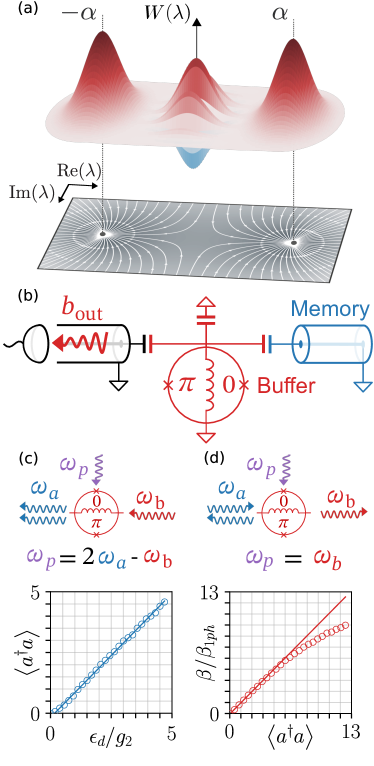
Figure 1: Encoding quantum information in a bistable dynamical system. (a) Semi-classical trajectories (solid lines, derived from Eq. (1)) converge towards two metastable states. Quantum information encoded in the manifold spanned by these states (the Wigner function corresponds to a coherent superposition state) inherit a protection against bit-flips. (b) Circuit implementation of our dynamical system (see text). (c) A pump (purple) and a buffer drive (red) combine through the ATS to inject photon pairs in the memory (blue). The reverse process that removes photon pairs is not represented. We measure (open circles) a linear increase (solid line) of the steady-state memory photon number (y-axis) versus drive amplitude (x-axis) (d) A pump at frequency $\omega_{b}$ (purple) mediates a longitudinal coupling between the memory (blue) and the buffer (red), a key ingredient for our quantum tomography protocol. We measure (open circles) the buffer amplitude (y-axis) versus the memory photon number (x-axis) reached after a displacement pulse. The deviation from the linear trend (solid line) is a signature of compression due to higher order processes.

Making the leap from classical to quantum information processing with dynamical bistable systems is difficult. Indeed, they owe their stability to friction - or dissipation - that dampens erroneous diffusion between states. However, friction commonly originates from interactions with an ensemble of degrees of freedom. This leaks information about the system, and quantum superpositions decohere into classical mixtures [11]. Surprisingly, there exists a type of dissipation, known as two-photon dissipation [12, 13, 14], that provides stability without inducing decoherence. Indeed, two-photon exchanges between an oscillator and its environment is expected to stabilize two coherent states with macroscopic bit-flip times, while permitting the preparation and manipulation of their quantum superpositions [14].

In practice, two-photon dissipation is implemented in a superconducting oscillator mode - the memory - that is coupled to a lossy buffer mode through a non linear Josephson element. In previous experiments, quantum tomography of the memory was performed via an ancillary system composed of a transmon and its readout resonator. While quantum superpositions of two metastable states were observed, the bit-flip time saturated in the millisecond range [15]. Cat-qubit implementations based on the Kerr effect reached similar timescales [16, 17]. In a recent experiment [18], this tomography apparatus was entirely removed and bit-flip times exceeding one hundred seconds were observed at the cost of forgoing the preparation and detection of quantum superpositions. This incriminating evidence motivated the removal of the ancillary transmon and the development of an alternative tomography procedure that does not break bit-flip protection.

In this experiment, we implement a cat-qubit with bit-flip times exceeding ten seconds, an improvement of four orders of magnitude over previous cat-qubit implementations, and six orders of magnitude over the lifetime of the photons composing the qubit. We observe phase-flip times greater than 490 ns, mainly limited by single-photon loss. We control the phase of coherent superpositions by rotating in a Zeno-blocked manifold [19], performing a $\pi$ rotation around $Z$ in 235 ns. We verify that this manipulation only marginally reduces the bit-flip time, maintaining it above ten seconds. This was made possible by implementing a quantum tomography protocol that requires no additional ancillary elements [20]. Indeed, the Josephson dipole that mediates two-photon dissipation is operated to map quantum observables of the memory onto the buffer. This experiment demonstrates the tomography and control of a cat-qubit without breaking bit-flip protection at the level of bit-flip times of ten seconds. However, further improvements in state preparation, measurement fidelities and single photon loss will be necessary before scaling to a fully-protected hardware-efficient logical qubit [6, 7, 8, 9].

Our dynamical system is well described by the following Hamiltonian and loss operator:

$$\mathbf{H}_{2ph} = {g_{2}^{*}}\mathbf{a}^{2}\mathbf{b}^{\dagger}+g_{2}{\mathbf{a}^{\dagger}}^{2}\mathbf{b}-\varepsilon_{d}^{*}\mathbf{b}-\varepsilon_{d}\mathbf{b}^{\dagger}\;,$$

$$\mathbf{L}_{b} = \sqrt{\kappa_{b}}\mathbf{b}\;,$$ (1)

where $\mathbf{a},\mathbf{b}$ are respectively the memory and buffer annihilation operators, $\varepsilon_{d}$ the amplitude of a resonant drive applied to the buffer, and $\kappa_{b}$ the buffer energy damping rate. Photon pairs are dissipated from the memory by converting them at rate $g_{2}$ to single photons in the buffer, which are then dissipated into the environment. In the absence of energy damping in the memory, the steady states of this system lie in a two-dimensional manifold [13] spanned by

$$\ket{\pm}_{\alpha}=(\ket{\alpha}\pm\ket{-\alpha})/\sqrt{\mathcal{N}_{\pm}}\;,$$ (2)

where $\mathcal{N}_{\pm}={2\pm 2\exp(-2\left|\alpha\right|^{2})}$ and $\ket{\alpha}$ is a coherent state of amplitude $\alpha$ that is controlled by the drive amplitude: $\alpha^{2}=\varepsilon_{d}/g_{2}^{*}$. The local convergence rate towards this manifold is denoted $\kappa_{\text{conf}}$ and in our parameter regime $\kappa_{\text{conf}}\approx\kappa_{b}/2$ (Sec. S6.3). The qubit encoded in this manifold owes its name - the cat-qubit [14] - to the fact that $\ket{\pm}_{\alpha}$ resemble Schrödinger cat states for $|\alpha|\gtrsim 1$ [21]. Its computational states are defined as $\ket{0/1}_{\alpha}=(\ket{+}_{\alpha}\pm\ket{-}_{\alpha})/\sqrt{2}\approx\ket{\pm\alpha}$, and its $X$ and $Z$ Pauli operator as $\mathbf{Z}_{\alpha}\approx\outerproduct{\alpha}{\alpha}-\outerproduct{-\alpha}{-\alpha}$ and $\mathbf{X}_{\alpha}\approx\outerproduct{\alpha}{-\alpha}+\outerproduct{-\alpha}{\alpha}$ up to errors that are exponentially small in $|\alpha|^{2}$.

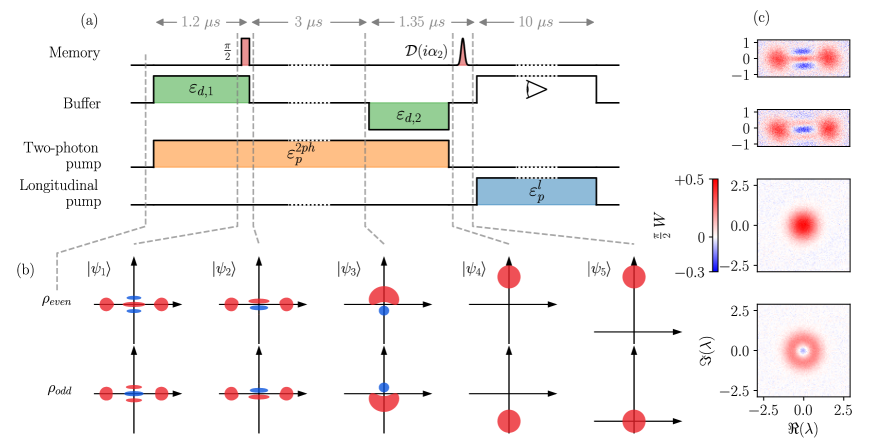
Figure 2: Quantum tomography protocol based on the holonomic gate [20]. (a) Pulse sequence for each control channel as a function of time. The parity of the memory is mapped onto photon number, which is measured through longitudinal coupling to the buffer (see text). (b) Cartoon of the memory Wigner function at each step (dashed lines) of the protocol for an even (top) and odd (bottom) initial state. (c) Measured Wigner functions of the memory initialized in : $\ket{+}_{\alpha},\ket{-}_{\alpha},\ket{0}$ and Fock state $\ket{1}$ (top to bottom), obtained by combining the photon parity measurement with simple memory displacements and an active memory reset (not shown, see Sec. S3.4). The first two images contain $250\times 100$ pixels averaged 5000 times, and the last two contain $100\times 100$ pixels averaged 70000 times. Their acquisition time is 2 and 12 hours respectively.

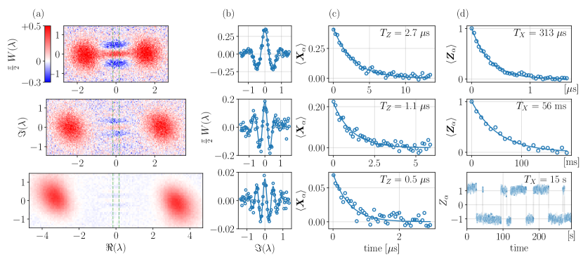
Figure 3: Cat-qubit phase-flip and bit-flip time measurements. Each row of figures represents a photon number $|\alpha|^{2}=2.5,5.6,11.3$ (top, middle, bottom). (a) Measured Wigner functions of the memory state prepared in $\ket{+}_{\alpha}$. Constraining these maps to sum to one sets an absolute scale for our parity measurement. (b) Integration of the measured Wigner functions (y-axis) over the window delimited by the green dashed lines in (a) versus the imaginary axis (x-axis). We fit the analytical formula of these oscillations [21] (solid lines) to the data (open circles). (c) Evolution of the expectation value of $\mathbf{X}_{\alpha}$ (y-axis) versus time (x-axis) for a memory initialized in the state $\ket{+}_{\alpha}$. The data (open circles) follow an exponential decay (blue solid line) from which we extract the phase-flip time $T_{Z}$. (d-top,middle) Expectation value of $\mathbf{Z}_{\alpha}$ (y-axis) versus time (x-axis). The data (open circles) follow an exponential decay (solid line) from which we extract the bit-flip time $T_{X}$. (d-bottom) Real-time trajectory cropped from the full data-set of the memory switching between $Z_{\alpha}=\pm 1$ (y-axis) versus time (x-axis). It is acquired by applying a drive on the memory and collecting the buffer fluorescence (solid line) (see Sec. S6.4).

States $\ket{\pm\alpha}$ are localized in opposite sides of phase-space (Fig. 1a), with exponentially small support overlap in $|\alpha|^{2}$. Therefore, even in the inevitable presence of losses, provided they are diffusive-like [22] and weak compared to $\kappa_{\text{conf}}$, the bit-flip time $T_{X}$ between $\ket{\pm\alpha}$ is expected to increase exponentially with $|\alpha|^{2}$ [15]. From $|\alpha|^{2}\approx 10$ onwards, timescales $T_{X}$ exceeding seconds are predicted in our parameter regime. Quantum superpositions of $\ket{\pm\alpha}$ are prepared by initializing the memory in the vacuum, and activating the two-photon exchange mechanism [13]. Since the dynamics of Eq. (1) conserves memory photon number parity, the state spontaneously dissipates towards $\ket{+}_{\alpha}$ on a timescale set by $\kappa_{\text{conf}}^{-1}$. The state then evolves into a classical statistical mixture of $\ket{\pm\alpha}$ at rate $\Gamma^{\kappa_{a}}_{Z}=2\kappa_{a}|\alpha|^{2}$ [21], where $\kappa_{a}$ is the memory energy damping rate. Therefore, the observation of quantum superpositions of metastable states with macroscopic bit-flip times requires that the decoherence rate verifies $\Gamma^{\kappa_{a}}_{Z}<\kappa_{\text{conf}}$ for $|\alpha^{2}|\approx 10$.

We implement the dynamics of Eq. (1) in a two-dimensional circuit quantum electrodynamics (cQED) architecture (Fig. 1b) [23] operated in a dilution refrigerator at 10 mK. The chip consists of a sapphire substrate on which we sputter a tantalum film [24], which is then patterned. The memory is a quarter wavelength coplanar waveguide resonator of frequency $\omega_{a}/2\pi=5.26$ GHz and decay rate $\kappa_{a}/2\pi=9.3$ kHz, corresponding to a lifetime of 17 $\mu$s. It is capacitively coupled to the buffer: an island shunted to ground through a nonlinear element called the ATS (Asymmetrically Threaded SQUID) [15], resonating at $\omega_{b}/2\pi=7.70$ GHz with decay rate $\kappa_{b}/2\pi=2.6$ MHz. The ATS is composed of a SQUID (Superconducting Quantum Interference Device) shunted in the middle by a kinetic inductance thus forming two loops. At the appropriate flux-bias point, this element induces the following nonlinear potential $U(\boldsymbol{\varphi})\approx-2E_{J}\epsilon_{p}(t)\sin(\boldsymbol{\varphi})$ [15], where $E_{J}$ is the Josephson energy of the SQUID junctions. Here, $\epsilon_{p}(t)=\varepsilon_{p}\cos(\omega_{p}t)$ is a flux-pump of amplitude $\varepsilon_{p}$ and angular frequency $\omega_{p}$, and $\boldsymbol{\varphi}$ is the phase drop across the ATS which is a linear combination of $\mathbf{a},\mathbf{a}^{\dagger},\mathbf{b},\mathbf{b}^{\dagger}$. Setting the pump frequency to $\omega_{p}=2\omega_{a}-\omega_{b}$ activates the desired third order process ${\mathbf{a}}^{2}\mathbf{b}^{\dagger}+{\mathbf{a}^{\dagger}}^{2}\mathbf{b}$ (Fig. 1c) at a rate $g_{2}$ that grows linearly with the pump amplitude. The latter is increased until $g_{2}$ is on par with $\kappa_{b}$, thereby maximizing $\kappa_{\text{conf}}$. We reach $g_{2}/2\pi=0.76$ MHz and $\kappa_{\text{conf}}/2\pi\approx 1.3$ MHz. For $|\alpha|^{2}\in[1.4,11.3]$, this places us in the favorable regime where $\Gamma^{\kappa_{a}}_{Z}/\kappa_{\text{conf}}\in[0.02,0.16]$.

Josephson circuits have been referred to as the Swiss army knife of microwave quantum optics [25]. Simply by switching the pump frequency, the behavior of a dipole can be dramatically changed. By setting the pump frequency to $\omega_{p}=\omega_{b}$ (Fig. 1d), the following processes are resonantly selected, to lowest order in $\boldsymbol{\varphi}$: $(\mathbf{b}+\mathbf{b}^{\dagger})$, $\mathbf{a}^{\dagger}\mathbf{a}(\mathbf{b}+\mathbf{b}^{\dagger})$ and $\mathbf{b}^{\dagger}\mathbf{b}(\mathbf{b}+\mathbf{b}^{\dagger})$. The first term $(\mathbf{b}+\mathbf{b}^{\dagger})$ is canceled by adding an additional drive of equal amplitude and opposite phase on the buffer. The second term $\mathbf{a}^{\dagger}\mathbf{a}(\mathbf{b}+\mathbf{b}^{\dagger})$ is a longitudinal coupling between the memory and the buffer [26, 27]. When $n_{a}$ photons are present in the memory, the buffer converges towards a coherent state of amplitude denoted $\beta_{1ph}\times n_{a}$. When cascaded with a heterodyne detection of the buffer, it constitutes a quantum non demolition (QND) measurement of the memory photon number. The third term $\mathbf{b}^{\dagger}\mathbf{b}(\mathbf{b}+\mathbf{b}^{\dagger})$ on the other hand is a parasitic interaction that limits the dynamical range of our detector. The longitudinal pump amplitude is chosen to maximize the detection efficiency over a dynamical range of 0 to about 10 photons in the memory. We reach a single shot fidelity of $89\%$ to distinguish between the vacuum and a coherent state containing 10 photons with an integration time of $10~{}\mu$s constrained by the memory lifetime (Sec. S3.2).

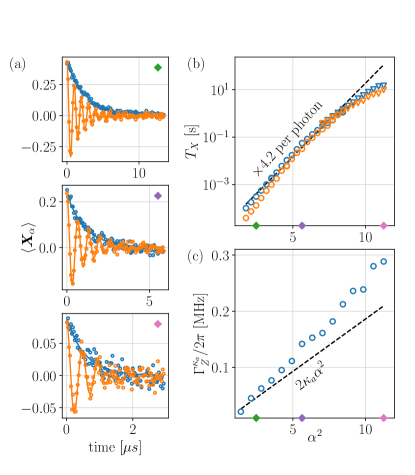
Figure 4: Quantum control that preserves bit-flip protection. (a) The cat-qubit is initialized in $\ket{+}_{\alpha}$ for $|\alpha^{2}|=2.5,5.6,11.3$ (top, middle, bottom), and the expectation value of $\mathbf{X}_{\alpha}$ (y-axis) is measured (open circles) versus time (x-axis). In the presence of a memory drive (orange), the cat-qubit undergoes coherent Zeno-blocked oscillations around its $Z$ axis. These oscillations decay exponentially with time. The data from Fig. 3b in the absence of the drive (blue) are superimposed for reference. (b) The bit-flip time (y-axis, log scale) increases exponentially with photon number (x-axis), multiplying by 4.2 for each added photon (dashed line). It is extracted from the average population transfer over time between $\ket{\pm\alpha}$ (circles), or from single real-time trajectories (triangles). The data is taken in the absence (blue) or presence (orange) of a memory drive. The same memory drive amplitudes $\epsilon_{Z}$ are applied in (a) and (b). (c) Dephasing rate (y-axis) as a function of photon number (x-axis). The data (open circles) only slightly deviate from the expected linear trend (dashed line).

We witness the quantum nature of the memory field through Wigner tomography [21]. The Wigner function is a quasi-probability distribution defined over the complex plane as $W(\lambda)=\frac{2}{\pi}\langle{\mathbf{D}_{\lambda}\mathbf{P}\mathbf{D}_{-\lambda}}\rangle$, which represents the normalized expectation value of the parity operator $\mathbf{P}=\exp(i\pi\mathbf{a}^{\dagger}\mathbf{a})$ for the state displaced by $\mathbf{D}_{\lambda}=\exp(\lambda\mathbf{a}^{\dagger}-\lambda^{*}\mathbf{a})$. This graphical representation can display negativities which unambiguously testify of the non-classical nature of the field state.

Our Wigner tomography protocol (Fig. 2) is based on the so-called holonomic gate proposed by Albert et. al [20]. All odd parity states are mapped onto the vacuum $\ket{0}$, and all even parity states onto a coherent state $\ket{\psi_{5}}=\ket{2i\alpha_{2}}$ where $2\alpha_{2}\approx 4.8$. The QND photon number measurement through longitudinal coupling then distinguishes between $\ket{0}$ and $\ket{2i\alpha_{2}}$, providing a photon number parity measurement. Our pulse sequence (Fig. 2a) alternates between memory drives, two-photon dissipation, buffer drives of various amplitudes and longitudinal coupling. We now describe it step by step (Fig. 2b). Let us assume that the memory is initially in an even parity state $\rho_{\text{even}}$. First, we activate a two-photon pump $\varepsilon_{p}^{2ph}$ and buffer drive $\varepsilon_{d,1}=g_{2}^{*}\alpha_{1}^{2}$ where $\alpha_{1}$ is real. By parity conservation, $\rho_{\text{even}}$ is mapped to the even state $\ket{\psi_{1}}=\ket{+}_{\alpha_{1}}$. Next, we add a memory drive along the imaginary axis. Two-photon dissipation confines the dynamics to the quantum manifold spanned by $\ket{\pm}_{\alpha_{1}}$. The added memory drive induces coherent Zeno-blocked oscillations around the cat-qubit $Z$ axis [19]. We tune the drive length to perform a $\pi/2$ rotation reaching the state $\ket{\psi_{2}}=(\ket{+}_{\alpha_{1}}+i\ket{-}_{\alpha_{1}})/\sqrt{2}$. Next, we turn off the memory and buffer drives while the two-photon pump remains active, thereby removing pairs of photons from $\ket{\psi_{2}}$. By parity conservation, $\ket{+}_{\alpha_{1}}$ is mapped to $\ket{0}$ and $\ket{-}_{\alpha_{1}}$ to $\ket{1}$. When this mapping is adiabatic with respect to $\kappa_{\text{conf}}^{-1}$ and fast compared to $\kappa_{a}^{-1}$, quantum superpositions are preserved, yielding $\ket{\psi_{3}}=(\ket{0}+i\ket{1})/\sqrt{2}$ [20]. In practice we use a square buffer drive of amplitude $\alpha_{1}\approx 1.6$ in an attempt to maximize the fidelity of the $\pi/2$ gate around $Z$, while minimizing the loss of coherence during these mappings. Next, maintaining the two-photon pump, we activate a buffer drive $\varepsilon_{d,2}=-g_{2}^{*}\alpha_{2}^{2}$ where $\alpha_{2}$ is real. This maps $\ket{0}\rightarrow\ket{+}_{i\alpha_{2}}$, $\ket{1}\rightarrow-i\ket{-}_{i\alpha_{2}}$ and following the same reasoning: $\ket{\psi_{3}}\rightarrow\ket{\psi_{4}}=\ket{i\alpha_{2}}$ [20]. Conversely, an odd parity $\rho_{\text{odd}}$ would be mapped to $\ket{-i\alpha_{2}}$. Information on the parity of $\rho_{\text{even/odd}}$ is now encoded on the amplitude of coherent states $\ket{\pm i\alpha_{2}}$. Finally, the two-photon pump is turned off, and the memory is displaced by $i\alpha_{2}$. The longitudinal pump $\varepsilon_{p}^{l}$ is activated to distinguish between 0 and $4|\alpha_{2}|^{2}$ photons in the memory by heterodyne detection of the buffer. Note that the value of $\alpha_{2}$ can be tuned to optimize the fidelity of the longitudinal readout. Preceding this entire sequence by a memory displacement of amplitude $\lambda$ therefore measures $W(\lambda)$. We demonstrate this tomography protocol by measuring the Wigner functions of the vacuum $\ket{0}$, Fock state $\ket{1}$, and $\ket{\pm}_{\alpha}$ (Fig. 2c). The vacuum is prepared simply by waiting for several $\kappa_{a}^{-1}$ for the memory to settle in its thermodynamic equilibrium. Preparing $\ket{+}_{\alpha}$ requires the activation of a two-photon pump and buffer drive for several $\kappa_{\text{conf}}^{-1}$. Preparing $\ket{-}_{\alpha}$ requires an additional memory drive to perform a full Zeno-blocked $\pi$ rotation. Finally, from this state, switching off the buffer drive while the two-photon pump remains active prepares Fock state $\ket{1}$ by parity conservation.

The measurements of phase-flip and bit-flip times of our cat-qubit are displayed in Fig. 3. We prepare $\ket{+}_{\alpha}$ for various average photon numbers $|\alpha|^{2}$ by starting from a memory mode in the vacuum, and activating the corresponding buffer drive amplitude and two-photon pump. This preparation takes 1 $\mu$s, which is longer than $1/\kappa_{\text{conf}}\approx 120$ ns, insuring sufficient time to reach the steady state manifold, and on par with $1/\Gamma^{\kappa_{a}}_{Z}\approx 490$ ns for the largest states at 11.3 photons, insuring the preservation of measurable quantum coherence. Using our novel tomography tool, we image the Wigner functions of these states and observe interference fringes that take negative values. While the contrast of these fringes reduces with $|\alpha|^{2}$, they remain visible up to $|\alpha|^{2}\approx 11.3$ photons (Fig. 3a,b). Note that in the cat-qubit code-space $\langle{\mathbf{X}_{\alpha}}\rangle=\langle{\mathbf{P}}\rangle$, and hence we extract the phase-flip time by monitoring the photon number parity decay over time. We measure phase-flip times ranging from $(\Gamma_{Z}^{\kappa_{a}})^{-1}=2.7~{}\mu$s for $|\alpha|^{2}=2.5$ to $(\Gamma_{Z}^{\kappa_{a}})^{-1}=490~{}$ns for $|\alpha|^{2}=11.3$ (Fig. 3c). Finally, we monitor the switching between $\ket{\pm\alpha}$ over time (Fig. 3d). To this end we prepare $\ket{+\alpha}$ by displacing the memory from the vacuum, before applying the two-photon pump and a buffer drive whose amplitude is adjusted to stabilize $\ket{\pm\alpha}$ for a variable time $t$. During this time, the state may switch to $\ket{-\alpha}$, causing a bit-flip. We detect the population of $\ket{\alpha}$ at time $t$ by setting the buffer drive to map $\ket{\pm\alpha}\rightarrow\ket{\pm\alpha^{\prime}}$ where $\alpha^{\prime}\approx 2.1$, then interrupting the pump and buffer drive, and finally displacing the memory by $\alpha^{\prime}$. This maps $\ket{-\alpha^{\prime}}\rightarrow\ket{0}$ and $\ket{\alpha^{\prime}}\rightarrow\ket{2\alpha^{\prime}}$. Next, we activate the longitudinal pump to distinguish between these two states. For bit-flip times exceeding $\approx 100$ ms, this method leads to impractically long acquisition times. Instead, for these long bit-flip times that occur at $|\alpha|^{2}\gtrsim 7$, we sample the real-time trajectory of the memory field. After initializing the memory in $\ket{\alpha}$ and activating the two-photon exchange, we apply a weak drive of amplitude $\varepsilon_{Z}$ on the memory for 250 $\mu$s every millisecond. This slightly displaces the state out of the steady state manifold. In response to this perturbation, the buffer develops an average field amplitude $\langle\mathbf{b}\rangle=\mp\frac{\varepsilon_{Z}}{2\alpha^{*}g_{2}}$ depending on the state $\ket{\pm\alpha}$ in the memory [28] (Sec. S6.4). This field is then integrated by heterodyne detection (Fig. 3d, bottom panel) for the pulse duration of $T_{\text{int}}=250~{}\mu$s. For $\alpha^{2}\gtrsim 7$, we have $T_{Z}\ll T_{\text{int}}\ll T_{X}$ and hence we observe bit-flip events in real time, so $T_{X}$ is well estimated from a single trace lasting $\approx 100~{}T_{X}$. Using these methods, we measure $T_{X}$ for $|\alpha|^{2}=2.5,5.6,11.3$, and observe a spectacular increase from $313~{}\mu$s, to $56$ ms, to 15 seconds.

We demonstrate quantum control of our cat-qubit and its impact on bit-flip protection in Fig. 4. After preparing the cat-qubit in $\ket{+}_{\alpha}$, we add a drive of amplitude $\varepsilon_{Z}$ on the memory mode. The interplay of this coherent drive and two-photon dissipation induces Zeno-blocked oscillations [19] at angular-frequency $\Omega_{Z}=2|\alpha|\varepsilon_{Z}$ [14], together with a drive-induced dephasing that increases with $\varepsilon_{Z}$ (Sec. S6.5). For $|\alpha^{2}|=11.3$, we observe a $\pi$ rotation in 235 ns. Since the benefit of the cat-qubit is to lighten the hardware overhead for error correction by sparing the need for active bit-flip correction, it is crucial to verify that our quantum manipulations do not break bit-flip protection. We measure the scaling of errors for $|\alpha|^{2}\in[1.4,11.3]$, a range on which we can measure both the phase-flip and bit-flip rates (Fig. 4b,c). We observe the bit-flip time multiply by 4.2 for every added photon, culminating at 15 seconds. Importantly, in the presence of the continuous memory drive, the bit-flip only slightly reduces, remaining above 10 seconds for $|\alpha|^{2}=11.3$. On the other hand, the dephasing rate $\Gamma^{\kappa_{a}}_{Z}$ increases linearly with $|\alpha|^{2}$, closely following the theoretical prediction $\Gamma^{\kappa_{a}}_{Z}=2\kappa_{a}|\alpha|^{2}$. Notably, despite the presence of the strong two-photon pump, the oscillator lifetime extracted from a linear fit to the data is only 25$\%$ larger than the one obtained from spectroscopy in the absence of the pump.

In conclusion, this experiment demonstrates quantum tomography and coherent control of a cat-qubit without breaking bit-flip protection up to bit-flip times of 10 seconds. This constitutes a $10^{4}$ improvement over other cat-qubit implementations, and a $10^{6}$ enhancement over the oscillator lifetime. We measure a phase-flip time of 490 ns, and perform a $\pi$ rotation around the $Z$ axis in 235 ns. Although we achieved $g_{2}/\kappa_{a}\approx 80\gg 1$, this ratio needs to be further increased to improve measurement fidelities and reduce state preparation and gate errors below the error correction threshold [6, 29]. Possible directions for progress are circuit engineering to increase $g_{2}$ [30, 31], optimized gate design [32, 28] and the integration of recent advances in nanofabrication [24, 33, 34] in order to improve our oscillator lifetime by at least one order of magnitude. With these improvements in hand, we envision assembling multiple cat-qubits in hardware-efficient error correcting architectures [6, 7, 8, 9], and operating them to correct phase-flips without breaking bit-flip protection.

Acknowledgements

We thank N. Frattini for his insight on applying the protocol of Albert et. al Phys. Rev. Lett. (2016) to Wigner tomography. We thank the SPEC at CEA Saclay for providing nano-fabrication facilities. This work was supported by the QuantERA grant QuCOS, by ANR 19-QUAN-0006-04. This project has received funding from the European Research Council (ERC) under the European Union’s Horizon 2020 research and innovation programme (grant agreements No. 851740 and No. 884762). This work has been funded by the French grants ANR-22-PETQ-0003 and ANR-22-PETQ-0006 under the ’France 2030 plan’.

Supplementary Material

S1 Device fabrication and wiring

In this section we describe the recipe we follow to fabricate the sample displayed in Fig. S1. The wiring diagram of the experiment is displayed in Fig. S2.

Wafer preparation

Our wafer is purchased from Starcryo and consists of a 2-inch, 430 $\mu$m-thick sapphire wafer, on which 200 nm of $\alpha$-phase tantalum were sputtered.

Circuit patterning

Large features of the circuit ($>5$ µm) are patterned using direct laser lithography, after coating with a 500 nm layer of positive resist (S1805). The exposed sample is developed in MF319 (1 min) and rinsed in deionized water (1 min), after which reactive ion etching (SF6, 0.02 mbar, 100 W) is used to transfer the pattern onto the Tantalum layer. Finally, the resist is stripped in an acetone bath (50°C, 20 min + 10 min sonication), followed by a 3 min oxygen plasma (0.02 mbar, 200 W).

Junction patterning

On top of the Tantalum circuit, Josephson junctions are patterned using the Dolan bridge technique. We coat the wafer with a bilayer consisting of MAA EL13 (650 nm, baked 3 min at 185°C) and PMMA A3 (120 nm, baked 30 min at 185°C). On top, a thin layer (20 nm) of conductive resist (Electra92) is spinned to improve charge-evacuation during lithography. Josephson junctions are patterned via electron beam lithography (20 keV). The wafer is developed in a 3:1, IPA:H₂O bath (6 °C, 2 min), and then rinsed in IPA (10 s) and blow-dried. Finally, a step of oxygen plasma ashing (10 s, 200 mbar, 75 W) allows to clean the mask from residual organic contaminants.

Junction deposition

Josephson junctions are evaporated via electron beam double-angle evaporation. First, a step of Argon milling (15 s, 5 mA, 500 V, $\pm$ 30°) is used to remove native Tantalum oxyde and assure good electrical contact between junctions and the Tantalum circuit. Then, two layers of aluminium (35 nm, 70 nm) are evaporated at angles $\pm$ 30°, with a step of static oxidation in between (15 O₂ - 75 Ar, 20 mbar, 10 min). Lift-off of the excess metal is done in acetone (50°C, 1 h, 2 min sonication) and an NMP-based remover (50°C, 10 min).

S2 Circuit Hamiltonian

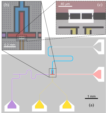
Figure S1: Layout and optical micrographs of the sample. (a) Layout displaying a quarter wave-length coplanar waveguide (CPW) resonator that supports the memory mode (blue). It is shunted to ground on its top end. The transmission line in its vicinity is unused in our experiment and is shunted to ground with a wirebond. On its bottom end, the memory oscillator couples capacitively to a superconducting island (red), corresponding to the buffer capacitance. The buffer is coupled from the left to a transmission line (purple) incorporating a Purcell filter. From this port we collect the buffer signals, and inject the buffer drive. A weakly coupled transmission line (pink) channels the memory drive and the cancellation tone for the longitudinal coupling into the circuit. The two symmetric lines (yellow) carry common and differential flux to bias the ATS, as well as the two-photon and longitudinal pump signals. (b) Optical micrograph in false color of the buffer island (red) and its surroundings. The tantalum film (light grey) is punctured with holes to avoid vortex trapping. The substrate (dark grey) is made out of sapphire. (c) Optical micrograph of the ATS fabricated in aluminum (white). The two small cross junctions (left and right) form a SQUID loop that is shunted in its center by a chain of 13 junctions.

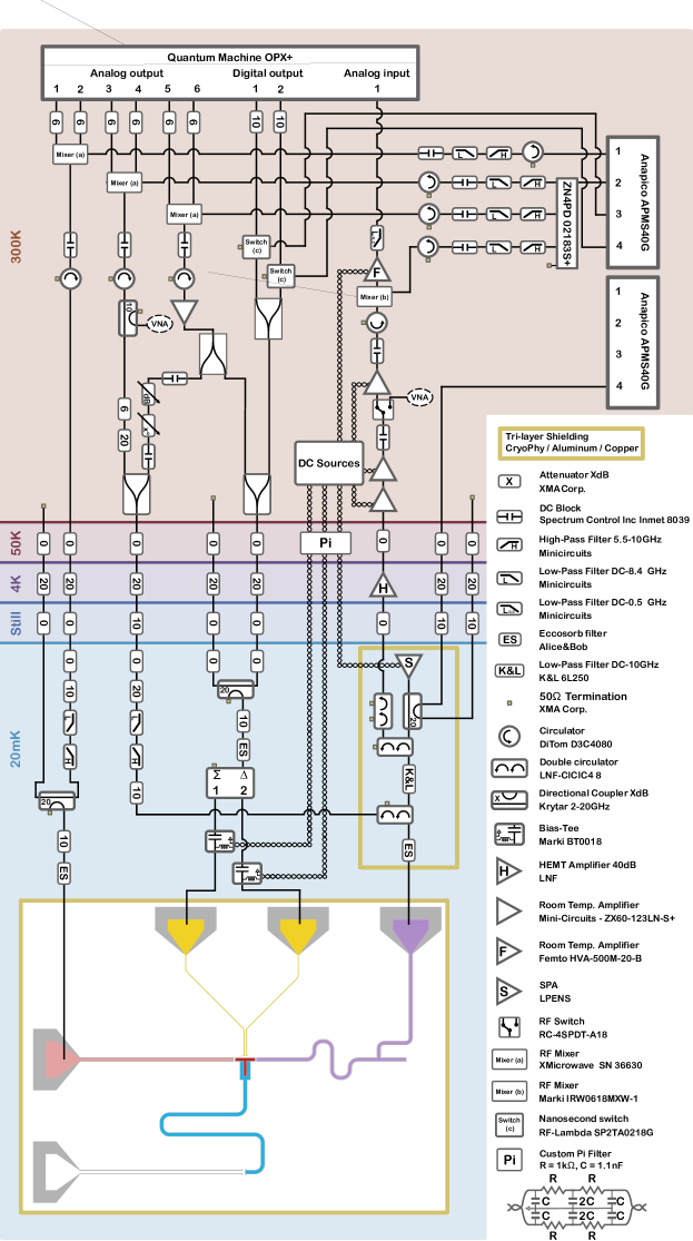
Figure S2: Wiring diagram of the experiment.

Our circuit, displayed in Fig. S1, is well described by the following Hamiltonian [15]:

$$\begin{split}\mathbf{H}_{\text{circuit}}&=\hbar\omega_{a,0}\mathbf{a}^{\dagger}\mathbf{a}+\hbar\omega_{b,0}\mathbf{b}^{\dagger}\mathbf{b}\\ &-2E_{J}\cos(\varphi_{\Sigma})\cos(\boldsymbol{\varphi}+\varphi_{\Delta})\\ &+2\Delta E_{J}\sin(\varphi_{\Sigma})\sin(\boldsymbol{\varphi}+\varphi_{\Delta})\\ \boldsymbol{\varphi}&=\varphi_{a}(\mathbf{a}+\mathbf{a}^{\dagger})+\varphi_{b}(\mathbf{b}+\mathbf{b}^{\dagger})\;.\end{split}$$ (S1)

The ATS is composed of two Josephson junctions of Josephson energies $E_{J1},E_{J2}$ in a SQUID loop configuration. We define $E_{J}=\frac{1}{2}(E_{J1}+E_{J2})$ and $\Delta E_{J}=\frac{1}{2}(E_{J1}-E_{J2})$. An inductive shunt splits the SQUID in a left and right loop that we thread with magnetic flux $\varphi_{L,R}$. We define the common and differential flux as $\varphi_{\Sigma,\Delta}=\frac{1}{2}(\varphi_{L}\pm\varphi_{R})$. Due to inevitable Josephson junction asymmetry $\Delta E_{J}$, the memory and buffer angular frequencies $\omega_{a,0},\omega_{b,0}$ slightly deviate from the mode frequencies $\omega_{a,\pm},\omega_{b,\pm}$ at the saddle points $(\varphi_{\Sigma},\varphi_{\Delta})=(\pi/2,\pm\pi/2)$. Indeed, $\omega_{a/b,\pm}\approx\omega_{a/b,0}\mp 2\Delta E_{J}\varphi_{a/b}^{2}$, where $\varphi_{a,b}$ are the zero point phase fluctuations of the buffer and memory across the ATS.

In order to pin down the value of each parameter entering this Hamiltonian, we run a 3D finite element electromagnatic simulation of our device in the absence of the two SQUID junctions, and where the ATS inductance consisting in a chain of 13 junctions is modeled by an inductive lumped element of energy $E_{L}$. Although room temperature resistance measurements provide an estimate of $E_{L}$ through the Ambegaokar-Baratoff formula, its precise value is determined by sweeping $E_{L}$ in the simulation and extracting the corresponding $\omega_{a,0},\omega_{b,0},\varphi_{a},\varphi_{b}$. We then pick the value of $E_{L}$ for which $\omega_{b,0}$ matches best the mean of the measured frequencies $\omega_{b,\pm}$ at the two saddle points. The difference between the measured frequencies at these two saddle points then sets the SQUID junctions asymmetry $\Delta E_{J}$. Finally fitting the measured buffer frequencies away from the saddle points sets the value of $E_{J}$. The comparison between the measured buffer frequencies and the ones extracted from Eq. (S1) is displayed in Fig. S3. The parameters entering the Hamiltonian are listed in table S1.

$\omega_{b,0}/2\pi$	7.70 GHz
$\varphi_{b}$	0.29
$\omega_{a,0}/2\pi$	5.26 GHz
$\varphi_{a}$	0.06
$E_{L}/h$	42.76 GHz
$E_{J}/h$	12.03 GHz
$\Delta E_{J}/h$	0.47 GHz

Table S1: Buffer, memory and ATS parameters entering Hamiltonian (S1) in order to produce the fit of Fig. S3.

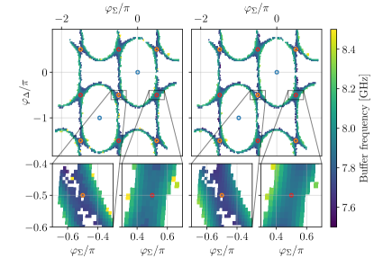
Figure S3: Measured (left) and simulated (right) buffer frequency (color) as a function of differential (x-axis) and common (y-axis) flux. Open orange and red circles mark the location of the two non-equivalent saddle points. The blue open circles point to the maximum of the flux map. The bottom panels are zooms around two nonequivalent saddle points. In the blank regions, the buffer is misaligned with its Purcell filter and is therefore too undercoupled to the transmission line to be detected. For the rest of the experiment, the flux is set to $(\varphi_{\Sigma},\varphi_{\Delta})=(-\pi/2,-\pi/2)$.

S3 Calibration of parametric pumps

S3.1 Parametric pumping of the ATS

In this experiment, the ATS is employed to mediate both a longitudinal coupling between the memory and the buffer, and to induce two-photon dissipation in the memory. To this end, we navigate the map displayed in Fig. S3 towards the saddle point $(\varphi_{\Sigma},\varphi_{\Delta})=(-\pi/2,-\pi/2)$, and keep this value fixed for the remainder of the experiment. At this bias point, the memory and buffer are first-order flux-insensitive and inherit small spurious Kerr interactions. For simplicity, we set $\Delta E_{J}$ to zero in this analysis and hence $\omega_{a/b,0}=\omega_{a/b,\pm}$. In the following, we denote $\omega_{a/b}$ the memory and buffer angular frequencies.

We combine this DC flux bias with an AC common flux pump of amplitude $\varepsilon_{p}$ and frequency $\omega_{p}$, yielding $\varphi_{\Sigma}=-\pi/2+\varepsilon_{p}\cos(\omega_{p}t)$ and $\varphi_{\Delta}=-\pi/2$. Injecting these expressions in Eq. (S1), we recover a nonlinear interaction term between the memory and buffer of the form $U(\boldsymbol{\varphi})=-2E_{J}\sin(\varepsilon_{p}\cos(\omega_{p}t))\sin(\boldsymbol{\varphi})$. In the regime where the pump amplitude $\varepsilon_{p}\ll 1$, $U(\boldsymbol{\varphi})\approx-2E_{J}\varepsilon_{p}\cos(\omega_{p}t)\sin(\boldsymbol{\varphi})$. Moreover since $\varphi_{a,b}\ll 1$, we may expand $\sin(\boldsymbol{\varphi})$ to third order :

$$U(\boldsymbol{\varphi})\approx-2E_{J}\varepsilon_{p}\cos(\omega_{p}t)(\boldsymbol{\varphi}-\frac{1}{6}\boldsymbol{\varphi}^{3})\;.$$ (S2)

S3.2 Longitudinal coupling

In this section we describe how the ATS is pumped to mediate a longitudinal coupling between the memory and the buffer, a crucial ingredient for our transmon-free quantum tomography protocol.

The amplitude of the pump tone employed for longitudinal coupling is denoted $\varepsilon^{l}_{p}$, and its frequency is to $\omega_{p}^{l}\approx\omega_{b}$. Performing a rotating wave approximation, the coupling term of Eq. (S2) reduces to

$$U_{\omega_{p}^{l}=\omega_{b}}(\boldsymbol{\varphi})/\hbar \approx g_{\text{lin}}(\mathbf{b}+\mathbf{b}^{\dagger})+g_{l}\mathbf{a}^{\dagger}\mathbf{a}(\mathbf{b}+\mathbf{b}^{\dagger})$$

$$+ g_{\text{sp}}\left({\mathbf{b}^{\dagger}}^{2}\mathbf{b}+\mathbf{b}^{\dagger}\mathbf{b}^{2}\right)\;.$$

The first term is a linear drive on the buffer of amplitude $g_{\text{lin}}=-E_{J}\varepsilon^{l}_{p}\varphi_{b}/\hbar$ (third order corrections in $\varphi_{a,b}$ are neglected). We cancel this term by applying an additional tone on the buffer, with equal amplitude and opposite phase, through a capacitively coupled port. The second term is the desired longitudinal coupling of strength $g_{l}=E_{J}\varepsilon^{l}_{p}\varphi_{a}^{2}\varphi_{b}/\hbar$. Finally, the third term, where $g_{\text{sp}}=\frac{1}{2}\varphi_{b}^{2}/\varphi_{a}^{2}g_{l}$, is a spurious term that limits the dynamical range of our detector. Future experiments will optimize the ratio $\varphi_{b}/\varphi_{a}$ to maximize the readout fidelity of the memory through this longitudinal coupling to the buffer. Considering only the longitudinal interaction, when there are exactly $n_{a}$ photons in the memory, the buffer converges to a coherent state of amplitude $\beta_{1ph}\times n_{a}$, where $\beta_{1ph}=-2ig_{l}/\kappa_{b}$.

In the following we describe the procedure we follow to calibrate (i) the pump frequency (ii) the amplitude of the cancellation tone and (iii) its phase. We sweep these parameters in a three-dimensional grid. For each combination we activate the pump and cancellation tones and record histograms of the buffer output both with and without an initial memory displacement. We select the combination of parameters that maximizes the Kullback–Leibler divergence between the two histograms. Finally, we record the buffer output as a function of the amplitude of the memory displacement (Fig. 1.d). We observe that the buffer output amplitude grows linearly with the number of photons in the memory up to about 5 photons, as expected from a longitudinal interaction. Above 5 photons, we observe a deviation from the linear dependence likely due to the spurious term $g_{\text{sp}}\left({\mathbf{b}^{\dagger}}^{2}\mathbf{b}+\mathbf{b}^{\dagger}\mathbf{b}^{2}\right)$. The power of the pump is chosen to maximize the span covered by the buffer amplitude over a window of 0 to 10 memory photons, which is the range of interest in this experiment. For the optimal pump power, we are able to distinguish between the vacuum and a coherent state in the memory containing 10 photons with a single-shot fidelity of 89% (Fig. S4).

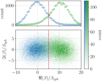
Figure S4: Measurement fidelity of the longitudinal readout: The memory is prepared in the vacuum (blue) or displaced to a coherent state containing an average photon number of 10 (green). The longitudinal pump is then activated, and the buffer output field is integrated over 10 $\mu$s. This measurement is repeated 20 000 times for each memory state preparation. (Bottom) Two-dimensional histogram of the real and imaginary quadratures of the buffer field. The histogram was rotated so that all the information on the memory state is encoded in the real quadrature. The histogram was also displaced so that the origin of the axis coincides with the center of the histogram corresponding to a memory in the vacuum. Finally the real and imaginary axis are re-scaled in units of average photon number present in the memory. (Top) Histogram of the real quadrature of the buffer output field, obtained by integrating the two-dimensional histogram over the imaginary quadrature. The vertical red dashed line is used to compute a single shot fidelity. We denote $P(L|0ph)$ the probability of measuring a data point on the left of the threshold, given a memory state prepared in the vacuum. Similarly, we denote $P(R|10ph)$ the probability of measuring a data point on the right of the threshold, given a memory state prepared in a coherent state containing 10 photons. We define the measurement fidelity as $(P(L|0ph)+P(R|10ph))/2$, and find 89%.

S3.3 Two-photon dissipation

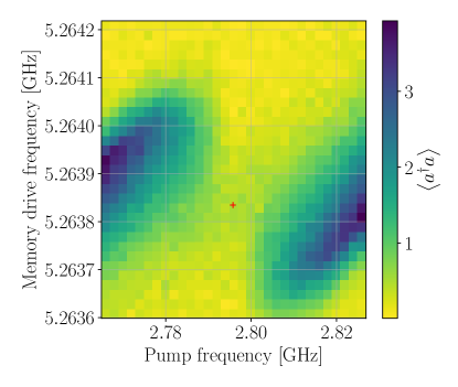
Figure S5: Calibration of the two-photon pump and memory drive frequencies. Photon number in the memory (color) as a function of the two-photon pump frequency $\omega_{p}^{2ph}$ (x-axis) and memory drive frequency $\omega_{Z}$ (y-axis). At the saddle point (red dot), the frequency matching condition $2\omega_{Z}-\omega_{p}^{2ph}=\omega_{b}$ is satisfied. Subsequently we set the buffer drive frequency to $\omega_{d}=2\omega_{Z}-\omega_{p}^{2ph}$.

In this section we describe how we implement two-photon dissipation in the memory, the mechanism at the core of the cat-qubit. The amplitude of the pump tone employed for two-photon dissipation is denoted $\varepsilon_{p}^{2ph}$ and its frequency is set to $\omega_{p}^{2ph}=2\omega_{a}-\omega_{b}$. Performing a rotating wave approximation on Eq. (S2), we find

$$U_{\omega_{p}^{2ph}=2\omega_{a}-\omega_{b}}(\boldsymbol{\varphi})/\hbar=g_{2}\left({\mathbf{a}^{2}\mathbf{b}}^{\dagger}+{\mathbf{a}^{\dagger}}^{2}\mathbf{b}\right)\;.$$

We recover the two-to-one exchange mechanism described in Eq. (1), where $g_{2}=\frac{1}{2}E_{J}\epsilon_{p}^{2ph}\varphi_{a}^{2}\varphi_{b}/\hbar$. For simplicity, $g_{2}$ is assumed to be a real number. Note that $g_{l}\propto g_{2}$, where $g_{l}$ is the longitudinal coupling derived in the previous section, and hence the performances of the longitudinal readout and the cat-qubit stabilization are directly linked. In the following, we simulate the dynamics of our two-photon dissipative system by numerically solving the Lindblad master equation:

$$\frac{d}{dt}{\rho} = -i\left[g_{2}\left(\mathbf{a}^{2}\mathbf{b}^{\dagger}+{\mathbf{a}^{\dagger}}^{2}\mathbf{b}\right)-\varepsilon_{d}^{*}\mathbf{b}-\varepsilon_{d}\mathbf{b}^{\dagger},\rho\right]$$

$$+ \kappa_{a}(1+n^{th}_{a})D[\mathbf{a}]\rho+\kappa_{a}n^{th}_{a}D[\mathbf{a}^{\dagger}]$$

$$+ \kappa_{b}(1+n^{th}_{b})D[\mathbf{b}]\rho+\kappa_{b}n^{th}_{b}D[\mathbf{b}^{\dagger}]\;,$$

where, $\rho$ is the buffer-memory density matrix, and $n^{th}_{a,b}$ are the memory and buffer thermal occupation numbers.

S3.3.1 Frequency calibration

The two-photon pump Stark-shifts the mode frequencies $\omega_{a,b}$. To calibrate the shifted frequencies, we activate the pump and vary its frequency $\omega_{p}^{2ph}$ in the vicinity of the frequency matching condition $2\omega_{a}-\omega_{b}$ , while applying a weak drive on the memory (which will later be used to perform Z rotations) of amplitude $\epsilon_{Z}$ whose frequency $\omega_{Z}$ is varied around $\omega_{a}$. For each value of this two-dimensional frequency sweep, we measure the memory photon number through longitudinal coupling to the buffer. This defines a two-dimensional map shown in Fig. S5, where $(\omega_{p}^{2ph},\omega_{Z})=(2\omega_{a}-\omega_{b},\omega_{a})$ is a saddle point. Indeed, at this operating point, the memory photon number is a balance between the memory drive strength, and the two-photon confinement rate. Detuning the two-photon pump results in a lower confinement rate, and hence a larger memory photon number. Conversely, detuning the memory drive reduces the memory photon number. Fitting the data to a second degree polynomial, we precisely locate the saddle point and pin down $\omega_{p}^{2ph}$ and $\omega_{Z}$. Finally, we set the buffer drive of amplitude $\epsilon_{d}$ to frequency $\omega_{d}=2\omega_{Z}-\omega_{p}^{2ph}$.

S3.3.2 Two-photon exchange rate calibration

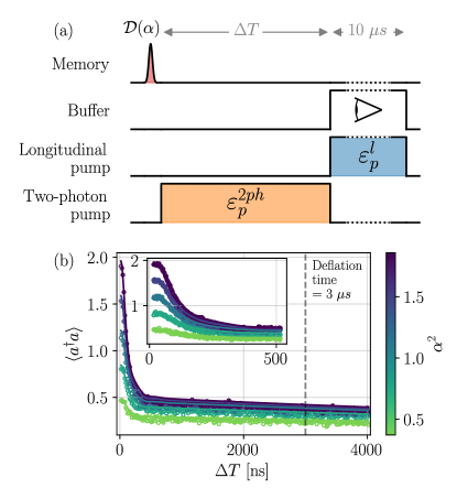
Figure S6: Calibration of the convergence time towards the $\ket{\pm}_{\alpha=0}$ manifold, colloquially referred to as the deflation time. (a) Pulse sequence : first, a coherent state of amplitude $\alpha$ in the memory is created. A two-photon pump is then activated for variable time $\Delta T$, and finally, the memory photon number is measured by longitudinal readout through the buffer. (b) Photon number (y-axis) as a function of $\Delta T$ (x-axis) for various initial coherent states $\ket{\alpha}$ (color). The data (open circles) are overlaid on theory curves obtained from solving the Lindblad master equation of Eq. (S3.3) with $\varepsilon_{d}=0$. The parameters entering the simulation are displayed in table S2. The only parameters that were varied to fit the data are $g_{2}$ and $n_{b}^{th}$. Other parameters were determined independently.

$g_{2}/2\pi$	0.763 MHz
$\kappa_{b}/2\pi$	2.6 MHz
$\kappa_{a}/2\pi$	9.3 kHz
$n_{a}^{th}$	10%
$n_{b}^{th}$	1.1%

Table S2: Parameters entering a Lindblad master equation to produce the fit of Fig. S6b.

To determine $g_{2}$, we measure the rate at which photons are removed from the memory mode by the two-photon dissipation mechanism. To do so, we implement the following pulse sequence (Fig. S6a): first the memory is displaced to a coherent state of amplitude $\alpha$, then the two-photon pump is activated for a variable time $\Delta T$, and finally, the memory photon number is measured by activating the longitudinal pump. The measured memory photon number versus time for various $\alpha$ is displayed in Fig. S6b. Two timescales are apparent. On a short timescale $1/\kappa_{\text{conf}}\approx 2/\kappa_{b}=120$ ns, pairs of photons are quickly removed from the memory until it is left in a mixture of $|0\rangle$ or $|1\rangle$ Fock states. At this stage, the number of photons $\langle a^{\dagger}a\rangle$ ranges from $1/2$ for initial state amplitudes $\alpha\gg 1$ down to $0$ when $\alpha=0$. Then, the remaining photon is dissipated into the memory bath on a longer timescale $1/\kappa_{a}$. The data are fitted by solving the master equation of the memory-buffer system (Eq. (S3.3)), with $\epsilon_{d}=0$, and $\rho(0)=\ket{\alpha}\bra{\alpha}$. The only fit parameters are the two-photon exchange rate and the thermal population of the buffer, for which we obtain $g_{2}/2\pi=763$ kHz and $n^{th}_{b}=1.1\%$. The dissipation rates $\kappa_{a}$ and $\kappa_{b}$ are measured independently using standard techniques. The number of photons in the memory (y-axis) and the thermal population of the memory $n^{th}_{a}$ are calibrated through Wigner tomography of the memory (Sec. S4).

S3.3.3 Cat state preparation

Since in this experiment we have entirely removed the transmon, we rely solely on the two-to-one photon exchange mechanism to generate quantum states. To this end, starting from the vacuum in the memory, we activate for a varying time $\Delta T$ both the two-photon pump and a buffer drive at various amplitudes $\varepsilon_{d}$. We then measure the memory photon number through longitudinal coupling to the buffer. The data are reported in Fig. S7. Three timescales are apparent. For $\Delta T\in[0,250~{}\text{ns}]$, we observe a rapid increase of photon number in the memory. Indeed, single photons from the buffer drive combine with the pump and pairs of photons are squeezed into the memory. For $\Delta T\in[250~{}\text{ns},600~{}\text{ns}]$, we observe damped oscillations in the memory photon number. Although we do not quantitatively understand the origin of these oscillations, they can be reproduced in simulation by adding a Kerr on the buffer, and a detuning of the pump and drive from the frequency matching condition. For $\Delta T\geq 600~{}\text{ns}$, the photon number reaches a plateau. This is expected when the memory has converged into the quantum manifold spanned by $\ket{\pm}_{\alpha}$. The specific state that is reached within this manifold depends on the initial state. Since the memory is initialized in the vacuum, the memory converges to the even cat $\ket{+}_{\alpha}$. However, due to inevitable losses in the memory, this state will evolve into a classical statistical mixture of $\ket{\pm}_{\alpha}$ at a rate $2|\alpha|^{2}\kappa_{a}$. The fidelity of preparation of $\ket{+}_{\alpha}$ is therefore maximized for the smallest time $\Delta T$ that insures the convergence of the memory in its steady state manifold. The cat states generated for Wigner tomography in Fig. 2c and Fig. 3a,b were prepared in $\Delta T=1~{}\mu$s. Those for the measurements of $\langle\mathbf{X}_{\alpha}\rangle$ in Fig. 3c and Fig. 4a were prepared in $\Delta T=400$ ns.

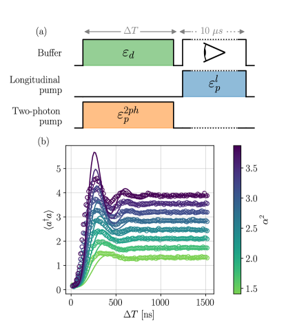
Figure S7: Calibration of the convergence time towards the $\ket{\pm}_{\alpha}$ manifold, colloquially referred to as the inflation time. (a) Pulse sequence : starting from the vacuum in the memory, the two-photon pump and buffer drive is activated for variable time $\Delta T$. The memory photon number is then measured by longitudinal readout through the buffer. (b) Photon number (y-axis) as a function of $\Delta T$ (x-axis) for drive amplitudes targeting various steady state memory photon numbers (color). The data (open circles) are overlaid with the results of a numerical simulation of Eq. (S3.3) with $\rho(0)=\ket{0}\bra{0}$, $\epsilon_{d}=\alpha^{2}g_{2}$ and no fit parameters. The parameters entering this simulation are summarized in Table. S2 have all been independently calibrated.

S3.4 Active memory reset

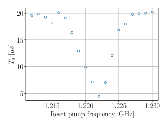
Figure S8: Calibration of the reset pump frequency. Memory lifetime $T_{a}$ (y-axis) versus the reset pump frequency (x-axis). The data (open circles) are extracted from a fit of the form $\exp(-t/T_{a})$ of the memory photon number decay versus time $t$ in the presence of the reset pump.

In the main text we acquire highly averaged and high resolution Wigner functions. The protocol for the generation and Wigner tomography of a memory state consists in a $\approx 15\mu$s pulse sequence followed by a long wait time for the memory to relax back to the vacuum. This wait time is typically $\approx 5/T_{a}$, where $T_{a}=1/\kappa_{a}$ is the memory lifetime. In order to reduce the acquisition time, we implement an active memory reset that reduces $T_{a}$, thereby accelerating the convergence of the memory to the vacuum. In this section we describe how we implement this reset mechanism.

We follow the same analysis as in Sec. S3.1, but we consider the term in $\Delta E_{J}$ that was previously neglected. At the flux saddle point, this term contributes a non-linear interaction of the form $U^{\Delta}(\boldsymbol{\varphi})=2\Delta E_{J}\cos(\varepsilon_{p}\cos(\omega_{p}t))\cos(\boldsymbol{\varphi})$. Assuming $\varepsilon_{p},|\boldsymbol{\varphi}|\ll 1$, we obtain

$$U^{\Delta}(\boldsymbol{\varphi})\approx 2\Delta E_{J}(1-\frac{1}{2}\varepsilon_{p}^{2}\cos(\omega_{p}t)^{2})(1-\frac{1}{2}\boldsymbol{\varphi}^{2})\;.$$ (S4)

The amplitude of the reset pump is denoted $\varepsilon_{p}^{\text{reset}}$ and its frequency is set to $\omega_{p}^{\text{reset}}=(\omega_{b}-\omega_{a})/2$. Performing a rotating wave approximation on Eq. (S4), we find

$$U^{\Delta}_{\omega_{p}=\omega_{p}^{\text{reset}}}(\boldsymbol{\varphi})/\hbar=g_{\text{reset}}(\mathbf{a}\mathbf{b}^{\dagger}+\mathbf{a}^{\dagger}\mathbf{b})\;,$$ (S5)

where $g_{\text{reset}}=\Delta E_{J}{\varepsilon_{p}^{\text{reset}}}^{2}\varphi_{a}\varphi_{b}/8\hbar$. We place ourselves in the regime where $g_{\text{reset}}\ll\kappa_{b}$, which induces a dissipation rate on the memory of the form $\kappa_{a}^{\text{reset}}=4g_{\text{reset}}^{2}/\kappa_{b}$.

In practice, we calibrate the reset pump by measuring the memory lifetime in the presence of the reset pump and vary its frequency (Fig. S8). When the reset pump frequency is far detuned from the frequency matching condition $(\omega_{b}-\omega_{a})/2$, the memory lifetime is unaffected by the pump, remaining around $20~{}\mu$s. However, when the pump frequency is set to $(\omega_{b}-\omega_{a})/2$, the memory lifetime drops to $\approx 5~{}\mu$s. Note that the buffer and memory frequencies that enter this frequency matching condition are those in the presence of the reset pump.

S4 Photon number calibration

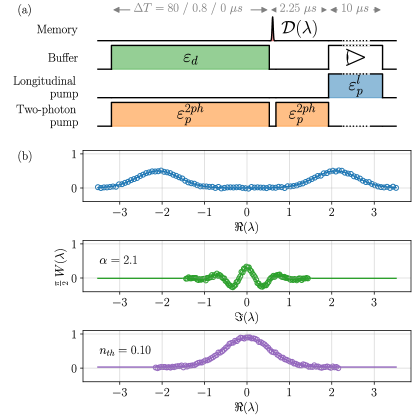
Figure S9: Photon number calibration. (a) Pulse sequence: a two-photon pump and buffer drive are active for $\Delta T=80,0.8,0~{}\mu$s, thereby preparing a statistical mixture of $\ket{\pm\alpha}$, a cat state $\ket{+}_{\alpha}$ and the thermal vacuum, respectively. Next, a Wigner tomography protocol is implemented (see text). (b) Cuts of the Wigner functions (y-axis) of these three states (top to bottom) along the real (top and bottom) and imaginary (middle) axis. The data (open circles) are overlaid with fits to the analytical formula displayed in Eq. (S4) (solid lines).

The readout protocol based on the memory-buffer longitudinal coupling yields a buffer signal proportional to the number of photons in the memory. Hence the proportionality constant must be calibrated. Even though the experiment shown Fig. S6 allows to calibrate it in principle, it is not very accurate. In order to access this crucial information, we elaborate a simple Wigner tomography tool. The signal to noise ratio of this method is lower than the one presented in the main text, however it requires less calibrations and is therefore more robust and easier to implement.

Wigner tomography:

Remarkably, since two-photon dissipation (with a buffer drive set to zero) removes photons in pairs, it maps all even parity states to the vacuum $\ket{n=0}$, and all odd parity states to Fock state $\ket{n=1}$. This maps parity to photon number, which is measurable through longitudinal coupling to the buffer. A memory displacement of amplitude $\lambda$ followed by a two-photon pump applied without buffer drive during $2~{}\mu$s (Fig. S6) therefore measures the Wigner function of the memory’s initial state $W(\lambda)$ (Fig. S9a). Single-photon losses during the measurement sequence and the overlap between the histograms of the longitudinal readout corresponding to $\ket{n=0}$ and $\ket{n=1}$ lead to a global reduction of the scale of the Wigner tomography.

Calibration:

We apply this tomography protocol to three different initial state preparations: (i) applying the two-photon pump and buffer drive for $\Delta T=80~{}\mu$s resulting in an almost equal statistical mixture of $\ket{\pm}_{\alpha}$, (ii) applying the two-photon pump and buffer drive for $\Delta T=800$ ns resulting in a mixture biased towards $\ket{+}_{\alpha}$ and (iii) no pump or drive at all, resulting in the vacuum state with some residual thermal population. Interestingly, note that while the thermal vacuum state displays a Wigner distribution that is broadened by thermal fluctuations, states (i) and (ii) are cooled into the cat-qubit manifold, and therefore the memory thermal occupation will impact the state reached within this manifold, but does not lead to thermal broadening. This asymmetry will be leveraged to calibrate the memory thermal occupation. Cuts of the Wigner functions of these three states are shown in Fig. S9.b, and overlaid with their fits to analytic formula [21]:

$$W_{\Delta T=80~{}\mu\text{s}}(\lambda_{r},0) = {A}\left(e^{-2(B\lambda_{r}-\alpha)^{2}}+e^{-2(B\lambda_{r}+\alpha)^{2}}\right)$$

$$W_{\Delta T=0.8~{}\mu\text{s}}(0,\lambda_{i}) = {C}e^{-2(B\lambda_{i})^{2}}\left(e^{-2\alpha^{2}}+\cos(4\alpha B\lambda_{i})\right)$$

$$W_{\Delta T=0~{}\mu\text{s}}(\lambda_{r},0) = {D}e^{-2(B\lambda_{r})^{2}/(2n_{th,a}+1)}\;,$$ (S6)

where $\lambda_{r,i}$ are the real and imaginary part of $\lambda$ and $A,B,C,D,\alpha,n_{a}^{th}$, as well as offsets, are free fit parameters. In essence, the frequency of the oscillations in (ii) sets an absolute scale $B$ for memory displacements in units of square root of photon number; the width of the Gaussian in (iii) sets the thermal population $n_{a}^{th}=10\%$ of the memory and the separation of the two Gaussians in (i) indicates the size of the cat-qubit $\alpha=2.1$. Furthermore, we do not observe a broadening of the two Gaussians in (i), which indicates a small thermal population $n^{b}_{th}$ of the buffer. Finally, the constants $A,C,D$ encode the different fidelities of state preparation and measurement.

S5 Quantum Zeno dynamics

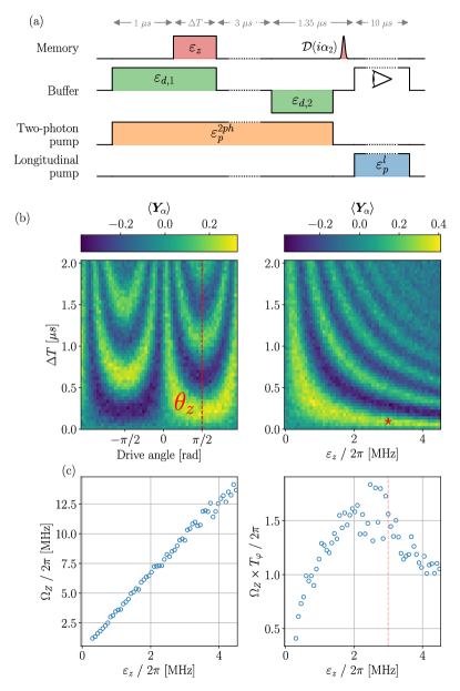
Figure S10: Quantum Zeno dynamics. (a) Pulse sequence: a two-photon pump and buffer drive prepare $\ket{+}_{\alpha}$. A memory drive is then activated with a variable phase and for a variable time $\Delta T$ inducing coherent rotations in the steady state manifold. The rest of the pulse sequence measures $\mathbf{Y}_{\alpha}$ as described in Fig. 2. (b-left) Buffer output proportional to the expectation value of $\mathbf{Y}_{\alpha}$ (color) as a function of the memory drive angle (x-axis) and duration (y-axis). The memory drive angle is set to maximize the oscillation frequency (red dashed line). (b-right) With the angle now calibrated, the memory drive amplitude is varied (x-axis) and the expectation value of $\mathbf{Y}_{\alpha}$ (color) is measured versus pulse duration (y-axis). (c-left) From this map we extract the oscillation frequency (y-axis) versus memory drive amplitude (x-axis). The data (open circles) follow the expected linear trend. (c-right) Number of coherent oscillations in units of oscillation frequency times fitted dephasing time (y-axis) versus memory drive amplitude $\varepsilon_{Z}$ (x-axis). The data (open circles) reach a maximum when $\varepsilon_{Z}$ balances rotation speed and induced dephasing (red star and dashed red line).

One of the main results of this work is to perform coherent oscillations of superpositions of metastable states with macroscopic bit-flip times. These oscillations are induced by the interplay of two-photon dissipation and a coherent drive on the memory. While the drive attempts to translate the memory state in phase space, two-photon dissipation continuously stabilizes the manifold spanned by $\ket{\pm}_{\alpha}$. As a result, when the phase of memory drive is 90 degrees out of phase with $\alpha$, we observe coherent oscillations between $\ket{\pm}_{\alpha}$. The coherent motion in a manifold stabilized by dissipation is known as quantum Zeno dynamics [35, 36, 37, 19].

In this section we describe the procedure we follow to calibrate the amplitude and phase of the memory drive (Fig. S10). Starting from a memory in vacuum, we implement the pulse sequence displayed in Fig.S10a, where the phase $\theta_{Z}$ and duration $\Delta T$ of the memory drive is varied. We observe $\langle Y_{\alpha}\rangle$ oscillating versus $\Delta T$, with an oscillation frequency that depends strongly on $\theta_{Z}$ (Fig. S10b). We identify the phase at witch the oscillation frequency is minimal with $\theta_{Z}=0$ mod $\pi$, that is, the memory is driven in phase with $\alpha$. On the other hand, we identify the phase at which the oscillation frequency of $\langle Y_{\alpha}\rangle$ is maximal with $\theta_{Z}=\pi/2$ mod $\pi$, that is, the memory drive is 90 degrees out of phase with $\alpha$. To optimize the $Z$ gate speed, we set $\theta_{Z}=\pi/2$ in the pulse sequence of Fig. 2a. Surprisingly, when we measure the evolution of $Z_{\alpha}$ in the presence of a memory drive with $\theta_{Z}=\pi/2$, we find that the $Z_{\alpha}$ population is skewed towards one of the two pointer states $\ket{\pm\alpha}$. Therefore, for the data of Fig. 4a,b, we tune $\theta_{Z}$ in a $\pm 15^{\circ}$ interval around $90^{\circ}$ to balance the population of $\ket{\pm\alpha}$. Understanding the origin of this deviation will be addressed in future work.

Having fixed the memory drive phase, we now vary its amplitude $\varepsilon_{Z}$. The data representing $\langle Y_{\alpha}\rangle$ as a function of drive amplitude and duration are displayed in Fig. S10c. Two features are visible. First, as the drive amplitude is increased, the frequency of the oscillation increases proportionally (Fig. S10d). Second, these oscillations decay faster as $\varepsilon_{Z}$ is increased, which is a manifestation of so-called non-adiabatic errors (Sec. S6.5). We plot the number of oscillations per decay time in Fig. S10e, and find that there is an optimal gate amplitude that balances gate duration and induced dephasing.

S6 Theory

In this section, we derive a semi-classical model for the dynamics described by Eq. (1) (Sec. S6.1). We then fully characterize the steady states of this semi-classical model (Sec. S6.2), derive the linearized evolution in their neighbourhood and compute the associated eigenvalues to extract the confinement rate (Sec. S6.3). Finally, we model our measurement scheme of real-time memory trajectories through the buffer in Sec. S6.4.

Note that a similar analysis was performed in Ref. [15] in the regime where $|g_{2}|\ll\kappa_{b}$. Here we generalize the analysis to arbitrary $g_{2}$ and $\kappa_{b}$.

S6.1 Semi-classical model

We start by writing the Hamiltonian of Eq.(1) with the substitution $\varepsilon_{d}=\alpha^{2}g_{2}^{*}$:

$$\mathbf{H}_{2ph} = g_{2}^{*}(\mathbf{a}^{2}-\alpha^{2})\mathbf{b}^{\dagger}+\mathrm{h.c.}\;.$$ (S7)

Next, using the Hamiltonian in the form given above, we compute the quantum Langevin equations associated to Eq. (1):

$$\dot{\mathbf{a}} = -2ig_{2}\mathbf{a}^{\dagger}\mathbf{b}$$

$$\dot{\mathbf{b}} = -ig_{2}^{*}(\mathbf{a}^{2}-\alpha^{2})-\frac{\kappa_{b}}{2}\mathbf{b}+\sqrt{\kappa_{b}}\mathbf{b}_{in}\;,$$ (S8)

where $\mathbf{b}_{in}$ is the incoming bath field on the buffer. Note that since we assume for simplicity that $\kappa_{a}$ is strictly zero in this analysis, the bath field on the memory does not enter this equation. The semi-classical approximation consists in replacing every operator in Eq. (S8) by its expectation value. We denote $a=\langle\mathbf{a}\rangle$ and $b=\langle\mathbf{b}\rangle$. Moreover, since $\langle\mathbf{b}_{\text{in}}\rangle=0$, we find:

$$\dot{a} = -2ig_{2}a^{*}b$$

$$\dot{b} = -ig_{2}^{*}(a^{2}-\alpha^{2})-\frac{\kappa_{b}}{2}b\;.$$ (S9)

S6.2 Steady states

The dynamics described in Eq. (S9) feature three fixed points :

$$(a,b)=(0,{2ig_{2}^{*}\alpha^{2}}/{\kappa_{b}})\;,(a,b)=(\alpha,0)\;,(a,b)=(-\alpha,0)\;.$$ (S10)

S6.2.1 Unstable equilibrium

Let us compute the linearized dynamics around $(a,b)=(0,{2ig_{2}^{*}\alpha^{2}}/{\kappa_{b}})$. To this end, we define $\delta a=a-0=a$ and $\delta b=b-2ig_{2}^{*}\alpha^{2}/{\kappa_{b}}$, and compute the dynamics of $\delta a,\delta b$ up to first order terms :

$$\left\{\begin{aligned} \delta\dot{a}&=\frac{4|g_{2}|^{2}}{\kappa_{b}}\alpha^{2}\delta a^{*}\\ \delta\dot{b}&=-\frac{\kappa_{b}}{2}\delta b\;.\end{aligned}\right.$$ (S11)

We thus see that $\real(\delta a)$ is unstable around this equilibrium.

S6.2.2 Stable equilibria

Let us compute the linearized dynamics around $(a,b)=(\alpha,0)$; the case of $a=-\alpha$ is similar. We define $\delta a=a-\alpha$ and $\delta b=b-0=b$, and compute the dynamics of $(\delta a,\delta b)$ up to first order terms :

$$\left\{\begin{aligned} \delta\dot{a}&=-2ig_{2}\alpha^{*}\,\delta b\\ \delta\dot{b}&=-2ig_{2}^{*}\alpha\delta a-\frac{\kappa_{b}}{2}\,\delta b\;.\end{aligned}\right.$$ (S12)

Notice that the structure of (S12) implies that we can decouple the dynamics of the real and imaginary parts of $\delta a$ and $\delta b$. We define the real quantities $x_{a,b},y_{a,b}$ such that $\delta a=x_{a}+iy_{a}$ and $\delta b=x_{b}+iy_{b}$. For simplicity, we assume $g_{2}$ and $\alpha$ to be real. We then have

$$\begin{bmatrix}\dot{x}_{a}\\ \dot{y}_{b}\\ \dot{y}_{a}\\ \dot{x}_{b}\\ \end{bmatrix}=\begin{bmatrix}0&2g_{2}\alpha&0&0\\ -2g_{2}\alpha&-\frac{\kappa_{b}}{2}&0&0\\ 0&0&0&-2g_{2}\alpha\\ 0&0&2g_{2}\alpha&-\frac{\kappa_{b}}{2}\end{bmatrix}\begin{bmatrix}x_{a}\\ y_{b}\\ y_{a}\\ x_{b}\end{bmatrix}$$ (S13)

Since a matrix and its transpose have the same eigenvalues, the eigenvalues associated to this linearized dynamics are the same as the eigenvalues of :

$$A=\begin{bmatrix}0&2g_{2}\alpha\\ -2g_{2}\alpha&-\frac{\kappa_{b}}{2}\end{bmatrix}\;.$$ (S14)

Notice that $\det(A)=4g_{2}^{2}\alpha^{2}>0$ and $\tr(A)=-\frac{\kappa_{b}}{2}<0$ so that the real part of each eigenvalue of $A$ is always negative. We can thus already conclude that the equilibria $(a=\pm\alpha,\,b=0)$ are stable for all values of $\alpha,\,\kappa_{b},\,g_{2}$.

S6.3 Confinement rate

In this section we derive an expression for the confinement rate $\kappa_{\text{conf}}$ at which states locally converge towards the stable steady state $(a,b)=(\alpha,0)$ (the case $(a,b)=(-\alpha,0)$ is similar). Let us denote the characteristic polynomial of the matrix $A$ by

$$\chi_{A}(\lambda)=\det(\lambda I-A)=\lambda^{2}+\frac{\kappa_{b}}{2}\lambda+4g_{2}^{2}\alpha^{2}\;.$$

Its discriminant is given by

$$\Delta=\frac{\kappa_{b}^{2}}{4}-16g_{2}^{2}\alpha^{2}=\frac{\kappa_{b}^{2}}{4}\left(1-\left(\frac{8g_{2}\alpha}{\kappa_{b}}\right)^{2}\right)\;.$$

The critical value of the parameters (i.e. the frontier between real and complex conjugate eigenvalues) is thus given by the relation

$$\frac{8g_{2}\alpha}{\kappa_{b}}\biggr{\rvert}_{\text{critical}}=1\;.$$

S6.3.1 Sub-critical regime : $8g_{2}\alpha<\kappa_{b}$.

In this case, the eigenvalues are real and given by

$$\lambda_{\pm}=-\frac{\kappa_{b}}{4}\left(1\pm\sqrt{1-\left(\frac{8g_{2}\alpha}{\kappa_{b}}\right)^{2}}\right).$$

The local convergence rate $\kappa_{\text{conf}}$ is thus governed by the eigenvalue of least magnitude

$$\kappa_{\text{conf}}\biggr{\rvert}_{\text{sub-critical}}=-2\lambda_{-}=\frac{\kappa_{b}}{2}\left(1-\sqrt{1-\left(\frac{8g_{2}\alpha}{\kappa_{b}}\right)^{2}}\right).$$

where the factor 2 comes from the fact eq. (S12) describes the amplitudes dynamics whereas the convergence rate should be homologous to an energy decay rate. Note that in the limit $g_{2}\ll\kappa_{b}$, a first order approximation of the above value is

$$\kappa_{\text{conf}}\biggr{\rvert}_{g_{2}\ll\kappa_{b}}=\frac{16g_{2}^{2}\alpha^{2}}{\kappa_{b}}=4\kappa_{2}\alpha^{2}$$

where $\kappa_{2}=\frac{4g_{2}^{2}}{\kappa_{b}}$. We recover the value of $\kappa_{\text{conf}}$ obtained in [15] by a semi-classical analysis of the effective one mode model when $g_{2}\ll\kappa_{b}$, up to a factor 2 due to the new convention.

S6.3.2 Super-critical regime : $8g_{2}\alpha>\kappa_{b}$.

In this case, the eigenvalues are complex conjugate and given by

$$\lambda_{\pm}=-\frac{\kappa_{b}}{4}\left(1\pm i\sqrt{\left(\frac{8g_{2}\alpha}{\kappa_{b}}\right)^{2}-1}\right).$$

The local convergence rate is thus given by their shared real part

$$\kappa_{\text{conf}}\biggr{\rvert}_{\text{super-critical}}=-2\real(\lambda_{\pm})=\frac{\kappa_{b}}{2}$$

S6.3.3 Regime of the experiment:

In our experiment, $\kappa_{b}/2\pi=2.6~{}$MHz and $g_{2}/2\pi=1$ MHz so $\kappa_{b}/8g_{2}\approx 0.3$. Hence for $\alpha>0.3$, we are in the super-critical regime, and $\kappa_{\text{conf}}=\kappa_{b}/2$ as announced in the main text. A mathematical analysis of the case where $\alpha=0$ is ongoing.

S6.4 Memory trajectories

This section discusses the measurement technique employed in the main text to measure macroscopic bit-flip times. By weakly driving the memory mode, the system moves away from its steady state thus inducing a response on the buffer mode that contains information about the bit value $\pm\alpha$ of the memory state [28].

The Hamiltonian in the presence of the memory drive of amplitude $\varepsilon_{Z}$ is $\mathbf{H}_{2ph}+\mathbf{H}_{Z}$ where $\mathbf{H}_{Z}=\varepsilon_{Z}\mathbf{a}^{\dagger}+\varepsilon_{Z}^{*}\mathbf{a}$. Following the same steps leading to Eq.(S12), the local dynamics around $a=\pm\alpha$ and $b=0$ read:

$$\left\{\begin{aligned} \delta\dot{a}&=\mp 2ig_{2}\alpha^{*}\,\delta b-i\varepsilon_{Z}\\ \delta\dot{b}&=\mp 2ig_{2}^{*}\alpha\delta a-\frac{\kappa_{b}}{2}\,\delta b\;.\end{aligned}\right.$$ (S15)

In steady state: $\delta\dot{a}=\delta\dot{b}=0$. Solving for $\delta b=b=\langle\mathbf{b}\rangle$ in Eq. (S15), we find

$$\langle\mathbf{b}\rangle=\mp\frac{\varepsilon_{Z}}{2\alpha^{*}g_{2}}\;.$$ (S16)

Therefore, by collecting the buffer output field, a weak measurement on the memory bit value is performed. Note that driving the system harder (i.e increasing $\varepsilon_{Z}$) would result in a higher readout contrast, but would also activate higher-order effects such as the ones neglected in this linearized dynamics that could eventually induce bit-flips by displacing the memory too far from its steady state.

S6.5 Drive-induced dephasing

In the previous section, we have demonstrated that a memory drive leaks information about the memory state through the buffer output. Equivalently, this drive induces decoherence - or dephasing - on the memory state. In this section, we compute the rate $\Gamma_{Z}^{\varepsilon_{Z}}$ of this drive-induced dephasing. From Eq. (S16), we find that depending on the state of the memory $\ket{\pm\alpha}$, the buffer converges to a coherent pointer state of amplitude $b_{\pm}=\mp\frac{\varepsilon_{Z}}{2\alpha^{*}g_{2}}$. The buffer then continuously radiates a field proportional to these amplitudes at a rate $\kappa_{b}/2$. Following [38], the induced dephasing is related to the rate at which information is gained on the memory state. Namely [28]:

$$\Gamma_{Z}^{\varepsilon_{Z}} = \frac{\kappa_{b}}{2}|b_{+}-b_{-}|^{2}$$

$$= \frac{\kappa_{b}}{2}|\frac{\varepsilon_{Z}}{\alpha g_{2}}|^{2}\;.$$

References

- [1] John Guckenheimer and Philip Holmes. Nonlinear Oscillations, Dynamical Systems, and Bifurcations of Vector Fields, pages 1–65. Springer New York, New York, NY, 1983.
- [2] Hideo Mabuchi. Coherent-feedback control strategy to suppress spontaneous switching in ultralow power optical bistability. Applied Physics Letters, 98(19):193109, 05 2011.
- [3] P. R. Muppalla, O. Gargiulo, S. I. Mirzaei, B. Prasanna Venkatesh, M. L. Juan, L. Grünhaupt, I. M. Pop, and G. Kirchmair. Bistability in a mesoscopic josephson junction array resonator. Phys. Rev. B, 97:024518, Jan 2018.
- [4] Google. Suppressing quantum errors by scaling a surface code logical qubit. Nature, 614(7949):676–681, February 2023.
- [5] Michael A. Nielsen and Isaac L. Chuang. Quantum Computation and Quantum Information: 10th Anniversary Edition. Cambridge University Press, 2010.
- [6] Jérémie Guillaud and Mazyar Mirrahimi. Repetition cat qubits for fault-tolerant quantum computation. Physical Review X, 9(4), December 2019.
- [7] Shruti Puri, Lucas St-Jean, Jonathan A. Gross, Alexander Grimm, Nicholas E. Frattini, Pavithran S. Iyer, Anirudh Krishna, Steven Touzard, Liang Jiang, Alexandre Blais, Steven T. Flammia, and S. M. Girvin. Bias-preserving gates with stabilized cat qubits. Science Advances, 6(34), August 2020.
- [8] Andrew S. Darmawan, Benjamin J. Brown, Arne L. Grimsmo, David K. Tuckett, and Shruti Puri. Practical quantum error correction with the xzzx code and kerr-cat qubits. PRX Quantum, 2:030345, Sep 2021.
- [9] Christopher Chamberland, Kyungjoo Noh, Patricio Arrangoiz-Arriola, Earl T. Campbell, Connor T. Hann, Joseph Iverson, Harald Putterman, Thomas C. Bohdanowicz, Steven T. Flammia, Andrew Keller, Gil Refael, John Preskill, Liang Jiang, Amir H. Safavi-Naeini, Oskar Painter, and Fernando G.S.L. Brandão. Building a fault-tolerant quantum computer using concatenated cat codes. PRX Quantum, 3(1), February 2022.
- [10] Austin G. Fowler, Matteo Mariantoni, John M. Martinis, and Andrew N. Cleland. Surface codes: Towards practical large-scale quantum computation. Phys. Rev. A, 86:032324, Sep 2012.
- [11] Wojciech Hubert Zurek. Decoherence, einselection, and the quantum origins of the classical. Rev. Mod. Phys., 75:715–775, May 2003.
- [12] M. Wolinsky and H. J. Carmichael. Quantum noise in the parametric oscillator: From squeezed states to coherent-state superpositions. Phys. Rev. Lett., 60:1836–1839, May 1988.
- [13] Z. Leghtas, S. Touzard, I. M. Pop, A. Kou, B. Vlastakis, A. Petrenko, K. M. Sliwa, A. Narla, S. Shankar, M. J. Hatridge, M. Reagor, L. Frunzio, R. J. Schoelkopf, M. Mirrahimi, and M. H. Devoret. Confining the state of light to a quantum manifold by engineered two-photon loss. Science, 347(6224):853–857, 2015.
- [14] Mazyar Mirrahimi, Zaki Leghtas, Victor V. Albert, Steven Touzard, Robert J. Schoelkopf, Liang Jiang, and Michel H. Devoret. Dynamically protected cat-qubits: A new paradigm for universal quantum computation. New J. Phys., 16(4):045014, 2014.
- [15] Raphaël Lescanne, Marius Villiers, Théau Peronnin, Alain Sarlette, Matthieu Delbecq, Benjamin Huard, Takis Kontos, Mazyar Mirrahimi, and Zaki Leghtas. Exponential suppression of bit-flips in a qubit encoded in an oscillator. Nature Physics, 16(5):509–513, May 2020.
- [16] A. Grimm, N. E. Frattini, S. Puri, S. O. Mundhada, S. Touzard, M. Mirrahimi, S. M. Girvin, S. Shankar, and M. H. Devoret. Stabilization and operation of a kerr-cat qubit. Nature, 584(7820):205–209, August 2020.
- [17] Nicholas E. Frattini, Rodrigo G. Cortiñas, Jayameenakshi Venkatraman, Xu Xiao, Qile Su, Chan U Lei, Benjamin J. Chapman, Vidul R. Joshi, S. M. Girvin, Robert J. Schoelkopf, Shruti Puri, and Michel H. Devoret. The squeezed kerr oscillator: spectral kissing and phase-flip robustness, 2022.
- [18] C. Berdou, A. Murani, U. Réglade, W.C. Smith, M. Villiers, J. Palomo, M. Rosticher, A. Denis, P. Morfin, M. Delbecq, T. Kontos, N. Pankratova, F. Rautschke, T. Peronnin, L.-A. Sellem, P. Rouchon, A. Sarlette, M. Mirrahimi, P. Campagne-Ibarcq, S. Jezouin, R. Lescanne, and Z. Leghtas. One hundred second bit-flip time in a two-photon dissipative oscillator. PRX Quantum, 4:020350, Jun 2023.
- [19] S. Touzard, A. Grimm, Z. Leghtas, S. O. Mundhada, P. Reinhold, C. Axline, M. Reagor, K. Chou, J. Blumoff, K. M. Sliwa, S. Shankar, L. Frunzio, R. J. Schoelkopf, M. Mirrahimi, and M. H. Devoret. Coherent oscillations inside a quantum manifold stabilized by dissipation. Phys. Rev. X, 8:021005, Apr 2018.
- [20] Victor V. Albert, Chi Shu, Stefan Krastanov, Chao Shen, Ren-Bao Liu, Zhen-Biao Yang, Robert J. Schoelkopf, Mazyar Mirrahimi, Michel H. Devoret, and Liang Jiang. Holonomic quantum control with continuous variable systems. Phys. Rev. Lett., 116:140502, Apr 2016.
- [21] Serge Haroche and Jean-Michel Raimond. Exploring the Quantum: Atoms, Cavities, and Photons. Oxford University Press, 2006.
- [22] Daniel Gottesman, Alexei Kitaev, and John Preskill. Encoding a qubit in an oscillator. Phys. Rev. A, 64(1):012310, 2001.
- [23] S. M. Girvin. Circuit QED: Superconducting qubits coupled to microwave photons. In M. Devoret, B. Huard, R. Schoelkopf, and L. F. Cugliandolo, editors, Quantum Machines: Measurement and Control of Engineered Quantum Systems (Les Houches Session XCVI), pages 113–256. Oxford University Press, 2014.
- [24] Alexander P. M. Place, Lila V. H. Rodgers, Pranav Mundada, Basil M. Smitham, Mattias Fitzpatrick, Zhaoqi Leng, Anjali Premkumar, Jacob Bryon, Andrei Vrajitoarea, Sara Sussman, Guangming Cheng, Trisha Madhavan, Harshvardhan K. Babla, Xuan Hoang Le, Youqi Gang, Berthold Jäck, András Gyenis, Nan Yao, Robert J. Cava, Nathalie P. de Leon, and Andrew A. Houck. New material platform for superconducting transmon qubits with coherence times exceeding 0.3 milliseconds. Nature Communications, 12(1), March 2021.
- [25] Emmanuel Flurin. The Josephson mixer : a swiss army knife for microwave quantum optics. Ph.d. thesis, 2014.
- [26] Nicolas Didier, Jérôme Bourassa, and Alexandre Blais. Fast quantum nondemolition readout by parametric modulation of longitudinal qubit-oscillator interaction. Phys. Rev. Lett., 115:203601, Nov 2015.
- [27] S. Touzard, A. Kou, N. E. Frattini, V. V. Sivak, S. Puri, A. Grimm, L. Frunzio, S. Shankar, and M. H. Devoret. Gated conditional displacement readout of superconducting qubits. Phys. Rev. Lett., 122:080502, Feb 2019.
- [28] Ronan Gautier, Mazyar Mirrahimi, and Alain Sarlette. Designing high-fidelity gates for dissipative cat qubits, 2023.
- [29] Ronan Gautier, Alain Sarlette, and Mazyar Mirrahimi. Combined dissipative and hamiltonian confinement of cat qubits. PRX Quantum, 3:020339, May 2022.
- [30] Gianluca Aiello, Mathieu Féchant, Alexis Morvan, Julien Basset, Marco Aprili, Julien Gabelli, and Jérôme Estève. Quantum bath engineering of a high impedance microwave mode through quasiparticle tunneling. Nature Communications, 13(1), November 2022.
- [31] A Marquet, A Essig, J Cohen, N Cottet, A Murani, E Abertinale, S Dupouy, A Bienfait, T Peronnin, S Jezouin, R Lescanne, and B Huard. Cat qubit with 0.3 s bit-flip time owing to passive two photon dissipation, 2023.
- [32] Alec Eickbusch, Volodymyr Sivak, Andy Z. Ding, Salvatore S. Elder, Shantanu R. Jha, Jayameenakshi Venkatraman, Baptiste Royer, S. M. Girvin, Robert J. Schoelkopf, and Michel H. Devoret. Fast universal control of an oscillator with weak dispersive coupling to a qubit. Nature Physics, 18(12):1464–1469, October 2022.
- [33] Chenlu Wang, Xuegang Li, Huikai Xu, Zhiyuan Li, Junhua Wang, Zhen Yang, Zhenyu Mi, Xuehui Liang, Tang Su, Chuhong Yang, Guangyue Wang, Wenyan Wang, Yongchao Li, Mo Chen, Chengyao Li, Kehuan Linghu, Jiaxiu Han, Yingshan Zhang, Yulong Feng, Yu Song, Teng Ma, Jingning Zhang, Ruixia Wang, Peng Zhao, Weiyang Liu, Guangming Xue, Yirong Jin, and Haifeng Yu. Towards practical quantum computers: transmon qubit with a lifetime approaching 0.5 milliseconds. npj Quantum Information, 8(1), January 2022.
- [34] Shingo Kono, Jiahe Pan, Mahdi Chegnizadeh, Xuxin Wang, Amir Youssefi, Marco Scigliuzzo, and Tobias J. Kippenberg. Mechanically induced correlated errors on superconducting qubits with relaxation times exceeding 0.4 milliseconds, 2023.
- [35] Adrien Signoles, Adrien Facon, Dorian Grosso, Igor Dotsenko, Serge Haroche, Jean-Michel Raimond, Michel Brune, and Sébastien Gleyzes. Confined quantum zeno dynamics of a watched atomic arrow. Nature Physics, 10(10):715–719, August 2014.
- [36] F. Schäfer, I. Herrera, S. Cherukattil, C. Lovecchio, F.S. Cataliotti, F. Caruso, and A. Smerzi. Experimental realization of quantum zeno dynamics. Nature Communications, 5(1), January 2014.
- [37] L. Bretheau, P. Campagne-Ibarcq, E. Flurin, F. Mallet, and B. Huard. Quantum dynamics of an electromagnetic mode that cannot contain ¡i¿n¡/i¿ photons. Science, 348(6236):776–779, 2015.
- [38] Jay Gambetta, Alexandre Blais, D. I. Schuster, A. Wallraff, L. Frunzio, J. Majer, M. H. Devoret, S. M. Girvin, and R. J. Schoelkopf. Qubit-photon interactions in a cavity: Measurement-induced dephasing and number splitting. Phys. Rev. A, 74(4):042318, 2006.