The complete dynamics description of positively curved metrics in the Wallach flag manifold $\mathrm{SU}(3)/\mathrm{T}^{2}$

Abstract.

The family of invariant Riemannian manifolds in the Wallach flag manifold $\mathrm{SU}(3)/\mathrm{T}^{2}$ is described by three parameters $(x,y,z)$ of positive real numbers. By restricting such a family of metrics in the tetrahedron $\mathcal{T}:=x+y+z=1$, in this paper, we describe all regions $\mathcal{R}\subset\mathcal{T}$ admitting metrics with curvature properties varying from positive sectional curvature to positive scalar curvature, including positive intermediate curvature notion’s. We study the dynamics of such regions under the projected Ricci flow in the plane $(x,y)$, concluding sign curvature maintenance and escaping. In addition, we obtain some results for positive intermediate Ricci curvature for a path of metrics on fiber bundles over $\mathrm{SU}(3)/\mathrm{T}^{2}$, further studying its evolution under the Ricci flow on the base.

1. Introduction

Since the paper of Böhm and Wilking [BW07], which uses Ricci flow techniques to prove a sort of converse to the classical Bonnet–Meyers theorem, a folkloric aspect emerged on the dynamics of invariant metrics in the Wallach flag manifold $\mathrm{SU}(3)/\mathrm{T}^{2}$. To know, on the one hand, Theorem C in [BW07] deals with the compact manifold $M=\mathrm{Sp}(3)/\mathrm{Sp}(1)\times\mathrm{Sp}(1)\times\mathrm{Sp}(1)$, ensuring the existence of an invariant metric on such a homogeneous space which has positive sectional curvature and evolves under the so-called homogeneous Ricci flow in a metric with mixed Ricci curvature. On the other hand, however, the very prolific analysis in Böhm–Wilking’s paper cannot be straightforwardly applied to the manifold $\mathrm{SU}(3)/\mathrm{T}^{2}$, and Remark 3.2 in [BW07] states the existence of an invariant metric with positive Ricci curvature on the flag manifold $\mathrm{SU}(3)/\mathrm{T}^{2}$ that evolves under the homogeneous Ricci flow to a metric with mixed Ricci curvature. Some works appeared later, seeking to give different descriptions for such a metric evolution: [CW12, AN16]. We also observe that the study of geometric flows of invariant geometric structures on homogeneous spaces and Lie groups is a classic topic in Differential Geometry with recent developments. See, for instance, [Lau17, BFF20, AL19, BL19, LPV20, FR21, BLP22] and references therein.

In this paper, via a different tool, we provide a complete description of each invariant positively curved metric in $\mathrm{SU}(3)/\mathrm{T}^{2}$ for every notion of positive curvature interpolating between positive sectional curvature to positive scalar curvature, further studying the dynamic evolution of such metrics under a projected homogeneous Ricci flow. Theorem A below fully generalizes Theorem 1 in [AN16] for $\mathrm{SU(3)}/\mathrm{T}^{2}$ (there denoted by $W^{6}$), further extending Theorem 2 in the same reference for $W^{6}$, strengthen the results for all intermediate positive curvature notations. It also provides a complete description of Theorem 3 in [AN16] and fully generalizes [CGM23]. In Theorem A to interpolate between positive sectional curvature and positive Ricci curvature, we use the following concepts appearing in the literature, observing, however, that for the forthcoming definitions, there is no widely used notation/terminology.

Definition 1.

Given a point $p$ in a Riemannian manifold $(M,\textsl{g})$, and a collection $v,v_{1},\ldots,v_{d}$ of orthonormal vectors in $T_{p}M$, the $d^{\mathrm{th}}$-intermediate Ricci curvature at $p$ corresponding to this choice of vectors is defined to be $\operatorname{Ric}_{d}(v)=\sum_{i=1}^{d}K(v,v_{i}),$ where $K$ denotes the sectional curvature of g.

Definition 2 ($d\mathrm{th}$-intermediate positive Ricci curvature).

We say that a Riemannian manifold $(M,\textsl{g})$ has positive $d\mathrm{th}$-Ricci curvature if for every $p\in M$ and every choice of non-zero $d+1$-vectors $\{v,v_{1},\ldots,v_{d}\}$ where $\{v_{1},\ldots,v_{d}\}$ can be completed to generated an orthonormal frame in $T_{p}M$, it holds $\operatorname{Ric}_{d}(v)>0$.

It is remarkable that for an $n$-dimensional manifold, these curvatures interpolate between positive sectional curvature and positive Ricci curvature for $d$ ranging between $1$ and $n-1$. Quoting [Mou], the quantity presented in Definition 2 has been called “$d\mathrm{th}$-intermediate Ricci curvature”, “$d\mathrm{th}$-Ricci curvature”, “$d$-dimensional partial Ricci curvature”, and “$d$-mean curvature”. Considering this, we define

Definition 3.

Let $M^{n}$ be a $n$-dimensional manifold and fix $d\in\{1,\ldots,n-1\}$. We denote by $\operatorname{\mathcal{R}^{\mathrm{\,sec-Ric}}_{d}}$ the set of all admissible Riemannian metrics in $M^{n}$ which satisfies Definition 2, that is, that have $d\mathrm{th}$-intermediate positive Ricci curvature.

All invariant Riemannian metrics in the Wallach flag manifold $\mathrm{SU}(3)/\mathrm{T}^{2}$ can be described by three positive parameters. Hence, we can abuse notation and denote an invariant metric g in $\mathrm{SU}(3)/\mathrm{T}^{2}$ by $\textsl{g}=(x,y,z)$. On the other hand, we will always assume that $x+y+z=1$, so we only have two-parameter describing any invariant Riemannian metric, thus adopting the convention $\textsl{g}=(x,y,z)=(x,y,1-x-y)\equiv(x,y)$. We prove:

Theorem A.

Let $\mathrm{SU}(3)/\mathrm{T}^{2}$ be the $6$-dimensional Wallach flag manifold. Then for any $d\in\{1,\ldots,5\}$ the set $\operatorname{\mathcal{R}^{\mathrm{\,sec-Ric}}_{d}}$ is non-empty. Moreover,

1. for each $d\in\{1,2,3,5\}$, there exists an invariant Riemannian metric $\textsl{g}=(x_{0},y_{0})\in\operatorname{\mathcal{R}^{\mathrm{\,sec-Ric}}_{d}}$ and $t^{*}\in\mathbb{R}$ such that the projected homogeneous Ricci flow $\textsl{g}(t)=(x(t),y(t))$ with initial condition $\textsl{g}(0)=\textsl{g}$ belongs to $\operatorname{\mathcal{R}^{\mathrm{\,sec-Ric}}_{d}}$ for $t$-sufficiently small and $\textsl{g}(t)\not\in\operatorname{\mathcal{R}^{\mathrm{\,sec-Ric}}_{d}}$ for every $t$ in a neighborhood of $t^{*}$;

2. for each $d\in\{4,5\}$, there exists a region $\mathcal{R}_{d}\subseteq\operatorname{\mathcal{R}^{\mathrm{\,sec-Ric}}_{d}}$ such that for any invariant Riemannian metric $\textsl{g}=(x_{0},y_{0})\in\mathcal{R}_{d}$, the projected homogeneous Ricci flow $\textsl{g}(t)$ with initial condition $\textsl{g}(0)=\textsl{g}$ lies in $\mathcal{R}_{d}$ for every $t\in\mathbb{R}$. Moreover, $\mathcal{R}_{4}=\mathcal{R}^{\mathrm{\,sec-Ric}}_{4}$ (which is open) and $\mathcal{R}_{5}=\overline{\mathcal{R}_{4}}\setminus\{(1/2,0),(0,1/2),(1/2,1/2)\}\subsetneq\mathcal{R}^{\mathrm{\,sec-Ric}}_{5}$.

The projected Ricci flow’s global behavior and the sets’ dynamics $\operatorname{\mathcal{R}^{\mathrm{\,sec-Ric}}_{d}}$ under the flow described in Theorem A is illustrated in Figure 2.

Another related here-considered notion of intermeidate curvature condition is

Definition 4.

Let $M^{n}$ be a $n$-dimensional Riemannian manifold and let $d\leq n$. We say that the Ricci tensor of $M$ is $d$-positive if the sum of the $d$ smallest eigenvalues of the Ricci tensor is positive at all points.

It is worth pointing out that if $d$ ranges from $1,\ldots,n$, the condition given by Definition 4 interpolates between positive Ricci curvature and positive scalar curvature. Definition 5 below, to be further approached in Section 2.2, considers a generalization of Definition 4. We do not require that the Ricci tensor is $d$-positive. Instead, we look for positive combinations of the Ricci eigenvalues constrained by their multiplicity. Such a consideration encompasses Definition 4.

Definition 5.

Let $M^{n}$ be a $n$-dimensional Riemannian manifold. Fix $d\in\{1,\ldots,n\}$. We say that a Riemannian metric g on $M$ has positive $d$-curvature if, denoting by $\lambda_{1},\ldots,\lambda_{l}$ the distinct eigenvalues of the Ricci tensor $\operatorname{Ric}(\textsl{g})$ of g, for every collection of non-negative integers $\{(a_{1},\ldots,a_{l})\in\mathbb{N}^{l}:a_{1}+\ldots+a_{l}=d,~{}0\leq a_{j}\leq\mu(\lambda_{j})\}$ where $\mu(\lambda_{j})$ denotes the algebraic multiplicity of $\lambda_{j}$,

$$\sum_{j=1}^{l}a_{j}\lambda_{j}>0.$$

Definition 6.

Let $M^{n}$ be a $n$-dimensional manifold. Fix $d\in\{1,\ldots,n\}$. We denote the set of all admissible Riemannian metrics g on $M$ satisfying Definition 5 by $\operatorname{\mathcal{R}^{\mathrm{\,Ric-scal}}_{d}}$.

Remark 1.

Cautiousness must be taken since $d$-positivity of the Ricci tensor (Definition 4) is denoted by $\operatorname{Ric}_{d}>0$ in [CW20]. See [DVGÁM22, Section 2.2] or [CW20, p. 5] for further information.

We prove:

Theorem B.

Let $\mathrm{SU}(3)/\mathrm{T}^{2}$ be the $6$-dimensional Wallach flag manifold. Then for any $d\in\{1,\ldots,6\}$ the set $\operatorname{\mathcal{R}^{\mathrm{\,Ric-scal}}_{d}}$ is non-empty. Moreover, for each $d\in\{1,\ldots,6\}$,

1. there exists an invariant Riemannian metric $\textsl{g}=(x_{0},y_{0})\in\operatorname{\mathcal{R}^{\mathrm{\,Ric-scal}}_{d}}$ and $t^{*}\in{\mathbb{R}}$ such the projected homogeneous Ricci flow $\textsl{g}(t)=(x(t),y(t))$ with initial condition $\textsl{g}(0)=\textsl{g}$ belongs to $\operatorname{\mathcal{R}^{\mathrm{\,Ric-scal}}_{d}}$ for $t$-sufficiently small and $\textsl{g}(t)\not\in\operatorname{\mathcal{R}^{\mathrm{\,Ric-scal}}_{d}}$ for every $t$ in a neighborhood of $t^{*}$;

2. there exists an open region $\mathcal{R}\subsetneq\operatorname{\mathcal{R}^{\mathrm{\,Ric-scal}}_{d}}$ such that for any $\textsl{g}=(x_{0},y_{0})\in\mathcal{R}$, the homogeneous Ricci flow $\textsl{g}(t)$ with initial condition $\textsl{g}(0)=\textsl{g}$ lies in $\mathcal{R}_{d}$ for every $t\in\mathbb{R}$.

The projected Ricci flow’s global behavior and the sets’ dynamics $\operatorname{\mathcal{R}^{\mathrm{\,sec-Ric}}_{d}}$ under the flow described in Theorem B is illustrated in Figure 3.

Observe that Theorems A and B, when considered in perspective, makes us wonder whether we could lift positive intermediate curvature notions to fiber bundles, as in [RW22b]. Pursuing positive answers, the following could also be seen as analogous to Theorem A in [SW15].

Theorem C.

Let $\bar{\pi}:F\hookrightarrow M\rightarrow\mathrm{SU}(3)/\mathrm{T}^{2}$ be a fiber bundle with $\mathrm{SU}(3)$ as structure group. Assume that

1. a principal orbit of the $\mathrm{SU}(3)$-action on $F$ has as isotropy subgroup a maximal closed subgroup

2. fixed $1\leq d_{F}\leq\dim F-1$, $F$ admits a $\mathrm{SU}(3)$-invariant metric $\textsl{g}_{F}$ such that the induced metric $\bar{\textsl{g}}_{F}$ on the manifold part of quotient $F/\mathrm{SU}(3)$ lies in $\mathcal{R}^{\mathrm{\,sec-Ric}}_{d_{F}}$.

Then $\bar{\pi}$ admits a one-parameter family of Riemannian submersion metrics $\textsl{g}_{t}\in\mathcal{R}^{\mathrm{\,sec-Ric}}_{d_{F}+1}$ for $|t|$ sufficiently small. Moreover, there exists $t^{*}\in\mathbb{R}$ such that $\textsl{g}_{t}\not\in\mathcal{R}^{\mathrm{\,sec-Ric}}_{d_{F}+1}$ for every $t$ in a neighborhood of $t^{*}$.

It is worth noticing that the hypotheses in Theorem C restrict a lot of the possible principal orbits for the $\mathrm{SU}(3)$-action in $F$. To now, $F=\mathrm{SU}(3)/\mathrm{SO}(3),~{}\mathrm{SU}(3)/\mathrm{T}^{2},~{}\mathrm{SU}(3)/\mathrm{S}(\mathrm{U}(2)\times\mathrm{U}(1))$ and $\mathrm{SU}(3)$ over a discrete maximal closed subgroup, see Lemma 2.

Much work related to Definition 2 has been appearing, and recent attention to this subject can be noticed. For a complete list of references on the subject, we recommend [Mou]. Part of the idea of this paper was conceived looking at the examples built in [DVGÁM22] and explored in [GAZ23], studying the evolution of intermediate positive Ricci curvature (in the sense of Definition 2) on some generalized Wallach spaces, under the homogeneous Ricci flow. Their analyses closely follow the techniques developed in [BW07]. Of particular interest are also [KM23, GAZ23, RW22b, RW22a, Mou22].

2. The curvature formulae in $\mathrm{SU}(3)/\mathrm{T}^{2}$

We first give an explicit Weyl basis to $T_{o}\mathrm{SU}(3)/\mathrm{T}^{2}$ where $o=e\mathrm{T}^{2}$, being $e\in\mathrm{SU}(3)$ the unit element. More precisely, from the level of Lie algebra, let $\mathfrak{sl}(3;\mathbb{C})$ be the complex semisimple Lie algebra with compact real form $\mathfrak{su(3)}$, the Lie algebra of $\mathrm{SU}(3)$. It can be checked that $\mathfrak{t}^{2}$ is a Cartan sub-algebra of $\mathfrak{sl}(3;\mathbb{C})$, where $\mathfrak{t}^{2}=:\mathrm{Lie}(\mathrm{T}^{2})=T_{e}\mathrm{T}^{2}$.

Since $\mathfrak{t}^{2}$ is Abelian and the adjoint representation $\mathrm{ad}:\mathfrak{sl}(3;\mathbb{C})\rightarrow\mathfrak{gl}(\mathfrak{sl}(3;\mathbb{C})$ enjoys the property that the image $\mathrm{ad}(\mathfrak{t}^{2})$ consists of semisimple operators, being therefore simultaneously diagonalizable. Considering this, we thus decompose $\mathfrak{sl}(3;\mathbb{C})$ via appropriate invariant subspaces

(1) $$\mathfrak{sl}(3;\mathbb{C})=\bigoplus_{\lambda\in{\mathfrak{t}^{2}}^{*}}{\mathfrak{sl}(3;\mathbb{C})}_{\lambda},$$

where

(2) $${\mathfrak{sl}(3;\mathbb{C})}_{\lambda}:=\ker\left\{\mathrm{ad}(\mathfrak{t}^{2})-\lambda(\mathfrak{t}^{2})1:\mathfrak{sl}(3;\mathbb{C})\rightarrow\mathfrak{sl}(3;\mathbb{C})\right\},$$

for $h\in\mathfrak{t}^{2}$. Hence, a roots’ set is nothing but $\Pi:=\left\{\alpha\in{\mathfrak{t}^{2}}^{*}\setminus\{0\}:{\mathfrak{sl}(3;\mathbb{C})}_{\alpha}\not\equiv 0\right\}$.

We can extract from $\Pi$ a subset $\Pi^{+}$ completely characterized by both:

1. for each root $\alpha\in\Pi$ only one of $\pm\alpha$ belongs to $\Pi^{+}$

2. for each $\alpha,\beta\in\Pi^{+}$ necessarily $\alpha+\beta\in\Pi^{+}$ if $\alpha+\beta\in\Pi$.

To the set $\Pi^{+}$, we name subset of positive roots. We say that the subset $\Sigma\subset\Pi^{+}$ consists of the simple roots system if it collects the positive roots, which can not be written as a combination of two elements in $\Pi^{+}$.

Since $\mathfrak{h}$ is an Abelian Lie sub-algebra, we can pick a basis $\{H_{\alpha}:\alpha\in\Sigma\}$ to $\mathfrak{h}$ and complete it with $\{X_{\alpha}\in{\mathfrak{sl}(3;\mathbb{C})}_{\alpha}:\alpha\in\Pi\}$, generating what is called a Weyl basis of $\mathfrak{sl}(3;\mathbb{C})$: For any $\alpha,\beta\in\Pi$

1. $\mathcal{K}(X_{\alpha},X_{-\alpha}):=\mathrm{tr}~{}(\mathrm{ad}(X_{\alpha}\circ\mathrm{ad}(X_{-\alpha}))=1$

2. $[X_{\alpha},X_{\beta}]=m_{\alpha,\beta}X_{\alpha+\beta},~{}m_{\alpha,\beta}\in\mathbb{R}$,

where $\mathcal{K}$ is the Cartan–Killing form of $\mathfrak{g}$, see [SM21, p. 214]. Then $\mathfrak{sl}(3;\mathbb{C})$ decomposes into root subspaces:

$$\mathfrak{sl}(3;\mathbb{C})=\mathfrak{t}^{2}+\sum_{\alpha\in\Pi}\mathbb{C}X_{\alpha}.$$

It is straightforward from [SM21, Theorem 11.13, p. 224] that such a decomposition implies that the compact real form of $\mathfrak{su(3)}$ is given by

(3) $$\mathfrak{su(3)}=\sqrt{-1}\mathfrak{t}^{2}_{\mathbb{R}}+\sum_{\alpha\in\Pi^{+}}\mathrm{Span}_{\mathbb{R}}(X_{\alpha}+X_{-\alpha},\sqrt{-1}(X_{\alpha}-X_{-\alpha})).$$

Given the above information, it can be directly checked that a basis for the Lie algebra of $\mathrm{SU}(3)$ is given by

$$\frac{1}{2}\mathrm{diag}(2\mathrm{i},-\mathrm{i},\mathrm{i}),\ \frac{1}{2}\mathrm{diag}(0,\mathrm{i},-\mathrm{i}),\ \frac{1}{2}\mathrm{A}_{12},\ \frac{1}{2}\mathrm{S}_{12},\ \frac{1}{2}\mathrm{A}_{13},\ \frac{1}{2}\mathrm{S}_{13},\ \frac{1}{2}\mathrm{A}_{23},\ \frac{1}{2}\mathrm{S}_{23},$$

where $\mathrm{S}_{kj}$ is a symmetric matrix $3\times 3$ with $\mathrm{i}$ in inputs $kj$ and $jk$ and $0$ in the others. On the other hand, $\mathrm{A}_{jk}$ is an antisymmetric matrix $3\times 3$ that has $1$ on input $kj$ and $-1$ on input $jk$, $0$ elsewhere. Moreover, $\mathrm{i}=\sqrt{-1}$. Hence, we can extract a basis for the tangent space $T_{o}\mathrm{SU}(3)/\mathrm{T}^{2}$ by disregarding the matrices $\mathrm{diag}(2i,-\mathrm{i},\mathrm{i})$ and $\mathrm{diag}(0,\mathrm{i},-\mathrm{i})$. Furthermore, the $3$ components of the isotropy representation are generated by

$$\mathrm{span}_{\mathbb{R}}\left\{\frac{1}{2}\mathrm{A}_{jk},\frac{1}{2}\mathrm{S}_{jk}\right\}.$$

We digress a bit recalling that whenever a homogeneous space $M=G/K$ is reductive, with reductive decomposition $\mathfrak{g}=\mathfrak{k}\oplus\mathfrak{m}$ (that is, $[\mathfrak{k},\mathfrak{m}]\subset\mathfrak{m}$), then $\mathfrak{m}$ is $\operatorname{Ad}_{G}(K)$-invariant. Moreover, the map $\mathfrak{g}\to T_{b}(G/K)$ that assigns to $X\in\mathfrak{g}$ the induced tangent vector

$$X\cdot b=d/dt(\exp(tX)b)|_{t=0}$$

is surjective with kernel the isotropy subalgebra $\mathfrak{k}$. Using that $g\in G$ acts in tangent vectors by its differential, we have that

(4) $$g(X\cdot b)=(\operatorname{Ad}(g)X)\cdot gb.$$

Hence, the restriction $\mathfrak{m}\to T_{b}(G/K)$ of the above map is a linear isomorphism that intertwines the isotropy representation of $K$ in $T_{b}(G/K)$ with the adjoint representation of $G$ restricted to $K$ in $\mathfrak{m}$. This allows us to identify $T_{b}(G/K)=\mathfrak{m}$ and the $K$-isotropy representation with the $\operatorname{Ad}_{G}(K)$-representation.

Being $G$ a compact connected simple Lie group such that the isotropy representation of $G/K$ decomposes $\mathfrak{m}$ as

(5) $$\mathfrak{m}=\mathfrak{m}_{1}\oplus\ldots\oplus\mathfrak{m}_{n}$$

where $\mathfrak{m}_{1},\ldots,\mathfrak{m}_{n}$ are irreducible pairwise non-equivalent isotropy representations, all invariant metrics are given by

(6) $$g_{b} =x_{1}B_{1}+\ldots+x_{n}B_{n}$$

where $x_{i}>0$ and $B_{i}$ is the restriction of the (negative of the) Cartan-Killing form of $\mathfrak{g}$ to $\mathfrak{m}_{i}$. We also have

(7) $$\operatorname{Ric}(g_{b})=y_{1}B_{1}+\ldots+y_{n}B_{n}$$

where $y_{i}$ is a function of $x_{1},\ldots,x_{n}$.

Turning back to our example, which is a reductive homogeneous space, considering the previous discussion, an $\mathrm{Ad}(\mathrm{T}^{2})$-invariant inner product g is determined by three parameters $(x,y,z)$ characterized by

$$g\left(\frac{1}{2}\mathrm{A}_{12},\frac{1}{2}\mathrm{A}_{12}\right) =g\left(\frac{1}{2}\mathrm{S}_{12},\frac{1}{2}\mathrm{S}_{12}\right)=x,$$

$$g\left(\frac{1}{2}\mathrm{A}_{13},\frac{1}{2}\mathrm{A}_{13}\right) =g\left(\frac{1}{2}\mathrm{S}_{13},\frac{1}{2}\mathrm{S}_{13}\right)=y,$$

$$g\left(\frac{1}{2}\mathrm{A}_{23},\frac{1}{2}\mathrm{A}_{23}\right) =g\left(\frac{1}{2}\mathrm{S}_{23},\frac{1}{2}\mathrm{S}_{23}\right)=z.$$

We then redefine new basis to $\mathfrak{m}:=T_{0}(\mathrm{SU}(3)/\mathrm{T}^{2})$ by

$$X_{1}=\frac{1}{2\sqrt{x}}\mathrm{A}_{12},\ X_{2}=\frac{1}{2\sqrt{x}}\mathrm{S}_{12},\ X_{3}=\frac{1}{2\sqrt{y}}\mathrm{A}_{13},\ X_{4}=\frac{1}{2\sqrt{y}}\mathrm{S}_{13},\ X_{5}=\frac{1}{2\sqrt{z}}\mathrm{A}_{23},\ X_{6}=\frac{1}{2\sqrt{z}}\mathrm{S}_{23}.$$

Since the following formula holds for the sectional curvature of g (see [Bes87, Theorem 7.30, p. 183])

$$K(X,Y)=-\frac{3}{4}\|[X,Y]_{\mathfrak{m}}\|^{2}-\frac{1}{2}g([X,[X,Y]_{\mathfrak{g}}]_{\mathfrak{m}},Y)-\frac{1}{2}g([Y,[Y,X]_{\mathfrak{g}}])_{\mathfrak{m}},X)$$

$$+\|U(X,Y)\|^{2}-\textsl{g}(U(X,X),U(Y,Y)),$$

$$2\textsl{g}(U(X,Y),Z)=\textsl{g}([Z,X]_{\mathfrak{m}},Y)+\textsl{g}(X,[Z,Y]_{\mathfrak{m}})$$

we can set up the following table, where $C_{ij}^{k}$ denotes a structure constant, that is, $C_{ij}^{k}=\textsl{g}([X_{i},X_{j}],X_{k})$, and $K_{ij}$ the sectional curvature. Moreover, that for $(i,j)\neq(1,2),(3,4),(5,6)$ it holds that

$$K(X_{i},X_{j})=K_{ij}=-\frac{1}{2}C_{ij}^{k}C_{ik}^{j}-\frac{1}{2}C_{kj}^{i}C_{ij}^{k}-\frac{3}{4}(C_{ij}^{k})^{2}+\sum_{l=1}^{6}\frac{1}{4}\left(C_{li}^{j}+C_{lj}^{i}\right)^{2}-\sum_{l=1}^{6}C_{li}^{i}C_{lj}^{j}.$$

$\mathrm{i}$	$j$	$k$	$C_{ij}^{k}$	$K_{ij}$
$1$	$2$	$\mathrm{diag}(\mathrm{i},-\mathrm{i},0)$	$1/x$	$1/x$
$1$	$3$	$5$	$-\frac{\sqrt{z}}{2\sqrt{xy}}$	$-\frac{3}{16}\frac{z}{xy}+\frac{1}{8x}+\frac{1}{8y}+\frac{1}{16}\frac{(x-y)^{2}}{xyz}$
$1$	$4$	$6$	$-\frac{\sqrt{z}}{2\sqrt{xy}}$	$-\frac{3}{16}\frac{z}{xy}+\frac{1}{8x}+\frac{1}{8y}+\frac{1}{16}\frac{(x-y)^{2}}{xyz}$
$1$	$5$	$3$	$\frac{\sqrt{y}}{2\sqrt{xz}}$	$-\frac{3}{16}\frac{y}{xz}+\frac{1}{8x}+\frac{1}{8z}+\frac{1}{16}\frac{(z-x)^{2}}{xyz}$
$1$	$6$	$4$	$\frac{\sqrt{y}}{2\sqrt{xz}}$	$-\frac{3}{16}\frac{y}{xz}+\frac{1}{8x}+\frac{1}{8z}+\frac{1}{16}\frac{(z-x)^{2}}{xyz}$
$2$	$3$	$6$	$\frac{\sqrt{z}}{2\sqrt{xy}}$	$-\frac{3}{16}\frac{z}{xy}+\frac{1}{8x}+\frac{1}{8y}+\frac{1}{16}\frac{(y-x)^{2}}{xyz}$
$2$	$4$	$5$	$-\frac{\sqrt{z}}{2\sqrt{xy}}$	$-\frac{3}{16}\frac{z}{xy}+\frac{1}{8x}+\frac{1}{8y}+\frac{1}{16}\frac{(y-x)^{2}}{xyz}$
$2$	$5$	$4$	$\frac{\sqrt{y}}{2\sqrt{xz}}$	$-\frac{3}{16}\frac{y}{xz}+\frac{1}{8x}+\frac{1}{8z}+\frac{1}{8}\frac{(z-x)^{2}}{xyz}$
$2$	$6$	$3$	$-\frac{\sqrt{y}}{2\sqrt{xz}}$	$-\frac{3}{16}\frac{y}{xz}+\frac{1}{8x}+\frac{1}{8z}+\frac{1}{16}\frac{(z-x)^{2}}{xyz}$
$3$	$4$	$\mathrm{diag}(\mathrm{i},0,-\mathrm{i})$	$1/y$	$1/y$
$3$	$5$	$1$	$-\frac{\sqrt{x}}{2\sqrt{yz}}$	$-\frac{3}{16}\frac{x}{yz}+\frac{1}{8y}+\frac{1}{8z}+\frac{1}{16}\frac{(y-z)^{2}}{xyz}$
$3$	$6$	$2$	$\frac{\sqrt{x}}{2\sqrt{yz}}$	$-\frac{3}{16}\frac{x}{yz}+\frac{1}{8y}+\frac{1}{8z}+\frac{1}{16}\frac{(y-z)^{2}}{xyz}$
$4$	$5$	$2$	$-\frac{\sqrt{x}}{2\sqrt{yz}}$	$-\frac{3}{16}\frac{x}{yz}+\frac{1}{8y}+\frac{1}{8z}+\frac{1}{16}\frac{(y-z)^{2}}{xyz}$
$4$	$6$	$1$	$-\frac{\sqrt{x}}{2\sqrt{yz}}$	$-\frac{3}{16}\frac{x}{yz}+\frac{1}{8y}+\frac{1}{8z}+\frac{1}{16}\frac{(y-z)^{2}}{xyz}$
$5$	$6$	$\mathrm{diag}(0,\mathrm{i},-\mathrm{i})$	$1/z$	$1/z$

Table 1. Structure Constants and Sectional curvature of the basis’ elements

We can compute every notion of positive curvature from Table 1. Particularly, the Ricci curvature formula is given by $\operatorname{Ric}(X)=\sum_{\mathrm{i}=1}^{n}K(X,X_{i})$, straightforward computations from Table 1 leads to

(8) $$\operatorname{Ric}(X_{1})=\operatorname{Ric}(X_{2})= \frac{1}{2x}+\frac{1}{12}\left(\frac{x}{yz}-\frac{z}{xy}-\frac{y}{xz}\right),$$

(9) $$\operatorname{Ric}(X_{3})=\operatorname{Ric}(X_{4})= \frac{1}{2y}+\frac{1}{12}\left(-\frac{x}{yz}-\frac{z}{xy}+\frac{y}{xz}\right),$$

(10) $$\operatorname{Ric}(X_{5})=\operatorname{Ric}(X_{6})= \frac{1}{2z}+\frac{1}{12}\left(-\frac{x}{yz}+\frac{z}{xy}-\frac{y}{xz}\right).$$

Next, we discuss different notions of intermediate positive Ricci curvature, furnishing a common ground for subsequent analyses and (hence) to the proof of Theorems A, B.

2.1. Conditions to $\operatorname{\mathcal{R}^{\mathrm{\,sec-Ric}}_{d}}$: On the $d\mathrm{th}$-intermediate positive Ricci curvatures of left-invariant metrics on $\mathrm{SU}(3)/\mathrm{T}^{2}$ (interpotaling between positive sectional and positive Ricci curvature)

We now take advantage of Table 1 considering the symmetries appearing on the expressions for sectional curvature to get a simplified description of $d\mathrm{th}$-intermediate positive Ricci curvature (recall the Definition 2). Take $d$-vectors out of the basis $\{X_{1},\ldots,X_{6}\}\subset T_{o}\mathrm{SU}(3)/\mathrm{T}^{2}$ and pick any $1\leq d\leq 5$. To describe properly the $\operatorname{Ric}_{d}$-curvature on the direction of a given vector $X_{i}$ out of this basis, we must handle with some combinatorial quantities. To be more precise, observe that ensuring positivity of $\operatorname{Ric}_{d}(X_{i})$ in the sense of Definition 2, is related to collecting every possible combination appearing as below

$$\operatorname{Ric}_{d}(X_{i})=a_{12}\frac{1}{x}+b_{12}\left(-\frac{3}{16}\frac{z}{xy}+\frac{1}{8x}+\frac{1}{8y}+\frac{1}{16}\frac{(x-y)^{2}}{xyz}\right)+c_{12}\left(-\frac{3}{16}\frac{y}{xz}+\frac{1}{8x}+\frac{1}{8z}+\frac{1}{16}\frac{(z-x)^{2}}{xyz}\right),~{}i=1,2,$$

$$\operatorname{Ric}_{d}(X_{i})=a_{34}\frac{1}{y}+b_{34}\left(-\frac{3}{16}\frac{z}{xy}+\frac{1}{8x}+\frac{1}{8y}+\frac{1}{16}\frac{(y-x)^{2}}{xyz}\right)+c_{34}\left(-\frac{3}{16}\frac{x}{yz}+\frac{1}{8y}+\frac{1}{8z}+\frac{1}{16}\frac{(y-z)^{2}}{xyz}\right),~{}i=3,4,$$

$$\operatorname{Ric}_{d}(X_{i})=a_{56}\frac{1}{z}+b_{56}\left(-\frac{3}{16}\frac{y}{xz}+\frac{1}{8x}+\frac{1}{8z}+\frac{1}{16}\frac{(z-x)^{2}}{xyz}\right)+c_{56}\left(-\frac{3}{16}\frac{x}{yz}+\frac{1}{8y}+\frac{1}{8z}+\frac{1}{16}\frac{(y-z)^{2}}{xyz}\right),~{}i=5,6$$

where $a_{jj+1}\in\{0,1\}$, $b_{jj+1},c_{jj+1}\in\{0,1,2\}$ are such that $a_{jj+1}+b_{jj+1}+c_{jj+1}=d\leq 5$, with $(j,j+1)\in\{(1,2),(3,4),(5,6)\}$. That is, for instance, we have that $\operatorname{Ric}_{d}(X_{i})$ is positive for $i=1,2$ if, for every possible choice of $a_{12}\in\{0,1\},~{}b_{12},c_{12}\in\{0,1,2\}$ we have $\operatorname{Ric}_{d}(X_{i})>0$.

We picture that in this setting, it suffices to obtain positive $\operatorname{Ric}_{d}$ for every vector tangent to $\mathrm{SU}(3)/\mathrm{T}^{2}$ to look to the former expressions since $\operatorname{Ric}_{d}\left(\sum_{i=1}^{6}x^{i}X_{i}\right)=\sum_{i=1}^{6}(x^{i})^{2}\operatorname{Ric}_{d}(X_{i}).$ Therefore, to ensure the existence of some $1\leq d\leq 5$ with positive $\operatorname{Ric}_{d}$ curvature (in the sense of Definition 2), it is necessary and sufficient to find such a $d$ constrained as: For every $(j,j+1)\in\{(1,2),(3,4),(5,6)\}$ and every $a_{jj+1}\in\{0,1\},~{}b_{jj+1},c_{jj+1}\in\{0,1,2\}$ with $a_{jj+1}+b_{jj+1}+c_{jj+1}=d$ it holds that $\operatorname{Ric}_{d}(X_{i})>0$ for some $x,y,z$.

Summarily, fixed $d\in\{1,\ldots,5\}$, an invariant Riemannian metric $\textsl{g}=(x,y,1-x-y)$ in $\mathrm{SU}(3)/\mathrm{T}^{2}$ lies in $\operatorname{\mathcal{R}^{\mathrm{\,sec-Ric}}_{d}}$ if, and only if, for every $(j,j+1)\in\{(1,2),(3,4),(5,6)\}$, the scalar functions defined below, denote generically by $R^{jj+1}_{a,b,c}(x,y)$, are positive simultaneously for every $(a_{jj+1},b_{jj+1},c_{jj+1})\in\mathcal{O}_{d}:=\{(a,b,c)\in\{0,1\}\times\{0,1,2\}^{2}:a+b+c=d\}$

(11) $$R^{12}_{a,b,c}(x,y) :=a_{12}\frac{1}{x}+b_{12}\left(-\frac{3}{16}\frac{z}{xy}+\frac{1}{8x}+\frac{1}{8y}+\frac{1}{16}\frac{(x-y)^{2}}{xyz}\right)+c_{12}\left(-\frac{3}{16}\frac{y}{xz}+\frac{1}{8x}+\frac{1}{8z}+\frac{1}{16}\frac{(z-x)^{2}}{xyz}\right)$$

(12) $$R^{34}_{a,b,c}(x,y) :=a_{34}\frac{1}{y}+b_{34}\left(-\frac{3}{16}\frac{z}{xy}+\frac{1}{8x}+\frac{1}{8y}+\frac{1}{16}\frac{(y-x)^{2}}{xyz}\right)+c_{34}\left(-\frac{3}{16}\frac{x}{yz}+\frac{1}{8y}+\frac{1}{8z}+\frac{1}{16}\frac{(y-z)^{2}}{xyz}\right)$$

(13) $$R^{56}_{a,b,c}(x,y) :=a_{56}\frac{1}{z}+b_{56}\left(-\frac{3}{16}\frac{y}{xz}+\frac{1}{8x}+\frac{1}{8z}+\frac{1}{16}\frac{(z-x)^{2}}{xyz}\right)+c_{56}\left(-\frac{3}{16}\frac{x}{yz}+\frac{1}{8y}+\frac{1}{8z}+\frac{1}{16}\frac{(y-z)^{2}}{xyz}\right)$$

2.2. Conditions to $\operatorname{\mathcal{R}^{\mathrm{\,Ric-scal}}_{d}}$: On the intermediate positive Ricci curvatures of left-invariant metrics on $\mathrm{SU}(3)/\mathrm{T}^{2}$ (interpotaling between positive Ricci and positive scalar curvature)

Let us denote $\operatorname{Ric}_{\textsl{g}}(X_{1})=\operatorname{Ric}_{\textsl{g}}(X_{2}):=r_{x},~{}\operatorname{Ric}_{\textsl{g}}(X_{3})=\operatorname{Ric}_{\textsl{g}}(X_{4}):=r_{y}$ and $\operatorname{Ric}_{\textsl{g}}(X_{5})=\operatorname{Ric}_{\textsl{g}}(X_{6}):=r_{z}$. One recovers

$$r_{x} = \frac{1}{2x}+\frac{1}{12}\left(\frac{x}{yz}-\frac{z}{xy}-\frac{y}{xz}\right),$$

$$r_{y} = \frac{1}{2y}+\frac{1}{12}\left(-\frac{x}{yz}-\frac{z}{xy}+\frac{y}{xz}\right),$$

$$r_{z} = \frac{1}{2z}+\frac{1}{12}\left(-\frac{x}{yz}+\frac{z}{xy}-\frac{y}{xz}\right)$$

Let $a,b,c\in\mathbb{N}$ non-negative integers. Following Definition 5, in Section 4, we shall deal with positive intermediate Ricci curvature ranging from positive Ricci to positive scalar curvature. Aiming such a goal, let $d\in\{1,\ldots,6\}$ and consider the set $\mathcal{N}_{d}:=\{(a,b,c)\in\{0,1,2\}^{3}:a+b+c=d\}$. Define the scalar function $F_{a,b,c}(x,y,z):=ar_{x}+br_{y}+cr_{z}$. If for every $(a,b,c)\in\mathcal{N}_{d}$ one has $F_{a,b,c}(x,y,z)>0$, we say that g has $d$-positive intermediate curvature and $(x,y,z)\in\mathcal{\operatorname{\mathcal{R}^{\mathrm{\,Ric-scal}}_{d}}}$.

3. The projected homogeneous Ricci flow: Quick overview and the equations in $\mathrm{SU}(3)/\mathrm{T}^{2}$

We recall that a family of Riemannian metrics $g(t)$ in $M$ is called a Ricci flow if it satisfies

(14) $$\frac{\partial\textsl{g}}{\partial t}=-2\operatorname{Ric}(\textsl{g}).$$

For any compact connected and $n$-dimensional manifold $M$ one can consider (see [BWZ]):

(15) $$\frac{d\textsl{g}_{b}}{dt}=-2\left(\operatorname{Ric}(\textsl{g}_{b})-\frac{\mathrm{S}(\textsl{g}_{b})}{n}{\textsl{g}}_{b}\right)$$

which preserves the metrics with unit volume and is the gradient flow of $\textsl{g}_{b}\mapsto\mathrm{S}(\textsl{g}_{b})$ when restricted to such space. In particular, the normalized Ricci flow

(16) $$\frac{\partial\textsl{g}}{\partial t}=-2\left(\operatorname{Ric}(\textsl{g})-\frac{T(\textsl{g})}{n}\textsl{g}\right)$$

that preserves metrics of unit volume $V(\textsl{g})=\int_{M}dV_{\textsl{g}}$ necessarily decreases scalar curvature; where $dV_{\textsl{g}}$ is the Riemannian volume form and $T(\textsl{g})=\int_{M}\mathrm{S}(\textsl{g})dV_{\textsl{g}}$ is the total scalar curvature functional.

For any compact homogeneous space $M=G/K$ with connected isotropy subgroup $K$, a $G$-invariant metric g on $M$ is determined by its value $\textsl{g}_{b}$ at the origin $b=K$, which is a $\operatorname{Ad}_{G}(K)$-invariant inner product. Just like g, the Ricci tensor $\operatorname{Ric}(\textsl{g})$ and the scalar curvature $\mathrm{S}(\textsl{g})$ are also $G$-invariant and completely determined by their values at $b$, $\operatorname{Ric}(\textsl{g})_{b}=\operatorname{Ric}(\textsl{g}_{b})$, $\mathrm{S}(\textsl{g})_{b}=\mathrm{S}(\textsl{g}_{b})$. Taking this into account, the Ricci flow equation (14) becomes the autonomous ordinary differential equation known as the (non-normalized) homogeneous Ricci flow:

(17) $$\frac{dg_{b}}{dt}=-2\operatorname{Ric}(g_{b}).$$

The equilibria of (16) are precisely the metrics satisfying $\operatorname{Ric}(\textsl{g})=\lambda\textsl{g}$, $\lambda\in\mathbb{R}$, the so called Einstein metrics. On the other hand, the unit volume Einstein metrics are precisely the critical points of the functional $\mathrm{S}(\textsl{g})$ on the space of unit volume metrics (see [WZ]). Recalling equation (6) and (7) one derives that the Ricci flow (17) becomes the autonomous system of ordinary differential equations

(18) $$\frac{dx_{k}}{dt}=-2y_{k},\qquad\ k=1,\ldots,n.$$

It is always very convenient to rewrite the Ricci flow equation in terms of the Ricci operator $r(g)_{b}$, which is possible since $r(g)_{b}$ is invariant under the isotropy representation and hence $r(g)_{b}|_{\mathfrak{m}_{k}}$ is a multiple $r_{k}$ of the identity. One obtains

$$y_{k}=x_{k}r_{k}$$

and equation (18) becomes

(19) $$\frac{dx_{k}}{dt}=-2x_{k}r_{k}.$$

Recalling that he isotropy representation of $\mathrm{SU}(3)/\mathrm{T}^{2}$ decomposes into three irreducible and non-equivalent components:

$$\mathfrak{m}=\mathfrak{m}_{1}\oplus\mathfrak{m}_{2}\oplus\mathfrak{m}_{3}.$$

The Ricci tensor of an invariant metric $\textsl{g}=(x,y,z)$ is also invariant, and its components are given by (recall equations (8)-(10)):

$$r_{x} = \frac{1}{2x}+\frac{1}{12}\left(\frac{x}{yz}-\frac{z}{xy}-\frac{y}{xz}\right),$$

$$r_{y} = \frac{1}{2y}+\frac{1}{12}\left(-\frac{x}{yz}-\frac{z}{xy}+\frac{y}{xz}\right),$$

$$r_{z} = \frac{1}{2z}+\frac{1}{12}\left(-\frac{x}{yz}+\frac{z}{xy}-\frac{y}{xz}\right)$$

and the corresponding (unnormalized) Ricci flow equation is given by

(20) $$x^{\prime}=-2xr_{x},\quad y^{\prime}=-2yr_{y},\quad z^{\prime}=-2zr_{z}.$$

The projected Ricci flow is obtained by a suitable reparametrization of the time, obtaining an induced system of ODEs with phase-portrait on the set

$$\{(x,y,z)\in\mathbb{R}^{3}:x+y+z=1\}\cap{\mathbb{R}}^{3}_{+},$$

where $\mathbb{R}^{3}_{+}=\{(x,y,z)\in\mathbb{R}^{3}:x>0,y>0,z>0\}$, following of the projection on the $xy-$plane. The resulting system of ODEs is dynamically equivalent to the system (20) (Corollary 4.3 in [GMPa⁺22]).

Applying the analysis developed in [GMPa⁺22, Section 5], we arrive at the equations of the projected Ricci flow equation (see equation (31) in Section 5 of [GMPa⁺22]):

(21) $$\left\{\begin{array}[]{l}x^{\,\prime}={u(x,y)},\\ y^{\,\prime}={v(x,y)},\end{array}\right.\quad(x,y)\in T=\{(x,y)\in{\mathbb{R}}^{2}:\,x\geq 0,\,y\geq 0,\,x+y\leq 1\},$$

where

$$u(x,y)=2x\left(x^{2}(2-12y)-3x\left(4y^{2}-6y+1\right)+6y^{2}-6y+1\right),$$

and

$$v(x,y)=-2y(2y-1)\left(6x^{2}+6x(y-1)-y+1\right).$$

4. The global dynamics of invariant metrics on $\mathrm{SU}(3)/\mathrm{T}^{2}$ under the Ricci flow

Here we accomplish the proof of Theorems A–B. With this goal, let us begin recalling from Section 2.1 that, fixed $d\in\{1,\ldots,5\}$, then $\textsl{g}\in\operatorname{\mathcal{R}^{\mathrm{\,sec-Ric}}_{d}}$ if, and only if, the scalar functions $R^{jj+1}_{(a,b,c)}(x,y)$ obtained from g are simultaneously positive for every $(a,b,c)\in\mathcal{O}_{d}=\{(a,b,c)\in\{0,1\}\times\{0,1,2\}^{2}:a+b+c=d\}$ and every $(j,j+1)\in\{(1,2),(3,4),(5,6)\}$.

In contrast to it, understanding the existence of positively curved metrics for the curvature notions interpolating between Ricci and scalar curvature, that is, fixed $d\in\{1,\ldots,6\}$, finding $\textsl{g}\in\operatorname{\mathcal{R}^{\mathrm{\,Ric-scal}}_{d}}$, is reduced to, following Section 2.2, obtain $(x,y,z)$ for which $F_{a,b,c}(x,y,z)>0$ for every $a,b,c\in\mathcal{N}_{d}$, where $\mathcal{N}_{d}:=\{(a,b,c)\in\{0,1,2\}^{3}:a+b+c=d\}$,  $F_{a,b,c}(x,y,z):=ar_{x}+br_{y}+cr_{z}$ and

$$r_{x} = \frac{1}{2x}+\frac{1}{12}\left(\frac{x}{yz}-\frac{z}{xy}-\frac{y}{xz}\right),$$

$$r_{y} = \frac{1}{2y}+\frac{1}{12}\left(-\frac{x}{yz}-\frac{z}{xy}+\frac{y}{xz}\right),$$

$$r_{z} = \frac{1}{2z}+\frac{1}{12}\left(-\frac{x}{yz}+\frac{z}{xy}-\frac{y}{xz}\right)$$

In what follows, we describe the global dynamics of the vector field $F(x,y)=\big{(}u(x,y),v(x,y)\big{)}$ associated with differential system (21). The triangular domain $\mathcal{T}$ can be divided into four invariant triangles (see Figure 1), namely:

$$\mathcal{T}_{1}= \{(x,y)\in T:\,x+y\leq 1/2\},$$

$$\mathcal{T}_{2}= \{(x,y)\in T:\,x\geq 1/2\},$$

$$\mathcal{T}_{3}= \{(x,y)\in T:\,y\geq 1/2\},$$

and the central one

$$\mathcal{T}_{c}=\{(x,y)\in T:\,x\leq 1/2,\,y\leq 1/2,\,x+y\geq 1/2\}.$$

Denote the vertices of $\mathcal{T}$ by $O=(0,0)$, $P=(1,0)$, and $Q=(0,1).$ Also, denote the vertices of $\mathcal{T}_{c}$ by $L=(1/2,0),$ $M=(1/2,1/2),$ and $N=(0,1/2).$

The vertices $O,P,Q$ correspond to unstable star node equilibria. Indeed, for each $X\in\{O,P,Q\},$ the Jacobian matrix $dF(X)$ coincides with the identity matrix multiplied by $2$. The vertices $L,M,N$ correspond to stable star node equilibria. Indeed, for each $X\in\{L,M,N\},$ the Jacobian matrix $dF(X)$ coincides with the identity matrix multiplied by $-1$. Therefore, for each $X\in\{L,M,N,O,P,Q\},$ there exists a neighborhood $V\subset{\mathbb{R}}^{2}$ of $X$ such that vector field $F|_{V}$ is $C^{1}$ conjugated to the linear vector field $dF(X)\cdot(x,y).$ In particular, the closure of the orbits approaching to each one of these equilibria are transversal to each other at the equilibria. In addition, it is straightforward to see that heteroclinic orbits connect the unstable node $O$ to the stable nodes $L$ and $N$, the unstable node $P$ to the stable nodes $L$ and $M$, and the unstable node $Q$ to the stable nodes $M$ and $N$ (see Figure 1).

Besides the vertices $L,M,N,O,P,Q$, the vector field $F$ has four other equilibria. Three of them belonging to the sides of $\mathcal{T}_{c}$ and the last one in the interior of $\mathcal{T}_{c},$ namely $R=(1/4,1/4)$, $S=(1/2,1/4)$, $T=(1/4,1/2),$ and $U=(1/3,1/3).$ We remark that the points $R,S,T$ represents the Kähler-Einstein metrics; and the point $U$ represents the normal-Einstein metric.

The point $U$ corresponds to an unstable star node equilibrium. Indeed, the Jacobian matrix $dF(X)$ coincides with the identity matrix multiplied by $2/9$. Thus, the same comment above about the local $C^{1}$ conjugacy holds for $U$.

The points $R,S,$ and $T$ correspond to saddle equilibria. Indeed, for each $X\in\{R,S,T\},$ the Jacobian matrix $dF(X)$ has the eigenvalues $1/2$ and $-1/4$. In addition: the segments $\overline{OU}$, $\overline{PU}$, and $\overline{QU}$ correspond to the stable manifolds of $R,$ $S,$ and $T$, respectively; and the segments $\overline{NL}$, $\overline{LM}$, and $\overline{MN}$ correspond to the unstable manifolds of $R,$ $S,$ and $T$, respectively. In particular, the segments $\overline{RO},$ $\overline{RU},$ $\overline{SP},$ $\overline{SU},$ $\overline{TQ},$ and $\overline{TU}$ correspond to heteroclinic orbits connecting the unstable nodes with the saddles through the stable manifold; and the segments $\overline{RL},$ $\overline{RN},$ $\overline{SM},$ $\overline{SL}$, $\overline{TM},$ and $\overline{TN}$ correspond to heteroclinic orbits connecting the stable nodes with the saddles through the unstable manifold (see Figure 1).

Let $\alpha(X)$ and $\omega(X)$ denote, respectively, the $\alpha$ and $\omega$ limit sets of $X\in\mathcal{T}.$ Using Poincaré–Bendixson Theorem arguments, one can easily see that $\alpha(X)=\{O\}$ for any $X\in\mathcal{T}_{1}^{\circ}$; $\alpha(X)=\{P\}$ for any $X\in\mathcal{T}_{2}^{\circ}$; $\alpha(X)=\{Q\}$ for any $X\in\mathcal{T}_{3}^{\circ}$; and $\alpha(X)=\{U\}$ for any $X\in\mathcal{T}_{c}^{\circ}$. Also, one can easily see that $\omega(X)=\{N\}$ for any $X$ in the interior of the triangle $OUQ$; $\omega(X)=\{L\}$ for any $X$ in the interior of the triangle $OPU$; and $\omega(X)=\{M\}$ for any $X$ in the interior of the triangle $PQU$.

With the considerations above, we have completely described the asymptotic behavior of the trajectories with initial conditions lying on $\mathcal{T}$ (see Figure 1).

\begin{overpic}[height=170.71652pt]{phaseportrait.pdf} \put(0.0,0.0){$O$} \put(95.0,0.0){$P$} \put(3.0,97.0){$Q$} \put(47.0,0.0){$L$} \put(51.0,52.0){$M$} \put(-1.0,50.0){$N$} \put(25.0,20.0){$R$} \put(51.0,28.0){$S$} \put(27.0,52.0){$T$} \put(34.0,29.0){$U$} \end{overpic}

Figure 1. Phase portrait of the vector field $F$. Black circles correspond to the equilibria, whereas the continuous segments connecting them correspond to the heteroclinic orbits. The $\alpha$ and $\omega$ limit set of $F$ for any initial condition are completely described above.

4.1. Proof of Theorem A

Let $d\in\{1,2,3,4,5\}$ be fixed. Consider the family of scalar functions

$$R^{12}_{a,b,c}(x,y),~{}R^{34}_{a,b,c}(x,y),~{}R^{56}_{a,b,c}$$

explicitly defined in equations (11)-(13).

Accordingly, by drawing the curves $R^{jj+1}_{a,b,c}(x,y)=0$ over the triangle $\mathcal{T}$ (see Figure 2), we obtain the region $\operatorname{\mathcal{R}^{\mathrm{\,sec-Ric}}_{d}}$ as

$$\operatorname{\mathcal{R}^{\mathrm{\,sec-Ric}}_{d}}=\bigcup_{(j,j+1)\in\{(1,2),(3,4),(5,6)\}}\{(x,y)\in\mathcal{T}:\,R^{jj+1}_{a,b,c}(x,y)>0\,\,\forall\,\,(a,b,c)\in\mathcal{O}_{d}\}.$$

This region corresponds to the interior of the union of the colored and checkered regions in Figure 2.

For each $d\in\{1,2,3\},$ $\operatorname{\mathcal{R}^{\mathrm{\,sec-Ric}}_{d}}$ is contained in the interior of the central triangle, $\mathcal{T}_{c}^{\circ}$. In addition, the boundaries of $\operatorname{\mathcal{R}^{\mathrm{\,sec-Ric}}_{d}}$ are tangent to each other at the points $L,M,$ and $N.$ Moreover, at these points, such boundaries are tangent to the closure of the heteroclinic orbits $\overline{UL}$, $\overline{UM},$ and $\overline{UN}$ of $F$. Since, for each $\textsl{g}=(x_{0},y_{0})\in\operatorname{\mathcal{R}^{\mathrm{\,sec-Ric}}_{d}}\setminus(\overline{UL}\cup\overline{UM}\cup\overline{UN})$, $\omega(x_{0},y_{0})\in\{L,M,N\},$ then there must exists exists $t^{*}\in{\mathbb{R}}$ such that $\textsl{g}(t^{*})\not\in\operatorname{\mathcal{R}^{\mathrm{\,sec-Ric}}_{d}}$. Otherwise, the closure of the orbit of $F$ through $(x_{0},y_{0})$ would be tangent to either $\overline{UL}$, $\overline{UM},$ or $\overline{UN}$ at $L,$ $M,$ or $N$, which is impossible because $L,$ $M,$ and $N$ are star nodes equilibria and, as mentioned previously, the closure of the orbits approaching to each one of these equilibria are transversal to each other at the equilibria. It is worth mentioning that for $g=(x_{0},y_{0})\in(\overline{UL}\cup\overline{UM}\cup\overline{UN})\setminus\{L,M,N\}$, $g(t)\in\operatorname{\mathcal{R}^{\mathrm{\,sec-Ric}}_{d}}$ for every $t\in{\mathbb{R}}.$

Now, for $d=4,$ $\operatorname{\mathcal{R}^{\mathrm{\,sec-Ric}}_{d}}$ coincides with the interior of the central triangle, $\mathcal{T}_{c}^{\circ}$ (see Figure 2), which is invariant by the flow of $F.$ Therefore, for each $g=(x_{0},y_{0})\in\operatorname{\mathcal{R}^{\mathrm{\,sec-Ric}}_{d}}$, one has that $g(t)\in\operatorname{\mathcal{R}^{\mathrm{\,sec-Ric}}_{d}}$ for every $t\in{\mathbb{R}}.$

Finally, for $d=5,$ $\operatorname{\mathcal{R}^{\mathrm{\,sec-Ric}}_{d}}$ contains the interior of the central triangle, $\mathcal{T}_{c}^{\circ}$ (see Figure 2). Moreover, $\operatorname{\mathcal{R}^{\mathrm{\,sec-Ric}}_{d}}\setminus\mathcal{T}_{c}$ is nonempty. Thus, by taking $(x_{0},y_{0})\in\operatorname{\mathcal{R}^{\mathrm{\,sec-Ric}}_{d}}\setminus\mathcal{T}_{c},$ since $\alpha(x_{0},y_{0})\in\{O,P,Q\},$ we conclude that there exists $t^{*}\in{\mathbb{R}}$ such that $\textsl{g}(t)\not\in\operatorname{\mathcal{R}^{\mathrm{\,Ric-scal}}_{d}}$ for every $t$ in a neighborhood of $t^{*}$.

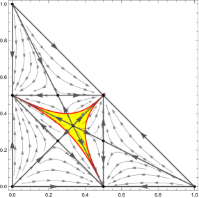
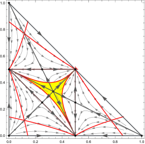
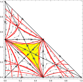
$d=1$	$d=2$	$d=3$
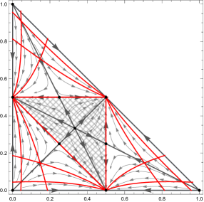
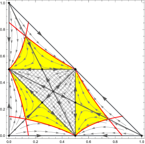
$d=4$	$d=5$

Figure 2. Phase portrait of the Projected Ricci flow is depicted jointly with the regions $\operatorname{\mathcal{R}^{\mathrm{\,sec-Ric}}_{d}}$ (see Definition 3). The yellow regions represent the metrics $g\in\operatorname{\mathcal{R}^{\mathrm{\,sec-Ric}}_{d}}$ that lose this property under the Ricci flow. Meanwhile, the checkered region ($d=4,5$) represents the metrics $g\in\operatorname{\mathcal{R}^{\mathrm{\,sec-Ric}}_{d}}$ for which the projected Ricci flow $g(t)$ with $g(0)=g$ satisfies $g(t)\in\operatorname{\mathcal{R}^{\mathrm{\,sec-Ric}}_{d}}$ for all $t\in\mathbb{R}$.

4.2. Proof of Theorem B

Let $d\in\{1,2,\ldots,6\}$ be fixed. For each $(a,b,c)\in\mathcal{N}_{d}$, we define the function $h_{a,b,c}(x,y):=F_{a,b,c}(x,y,1-x-y)$. Accordingly, by drawing the curves $h_{a,b,c}=0$ over the triangle $\mathcal{T},$ we obtain the region $\operatorname{\mathcal{R}^{\mathrm{\,Ric-scal}}_{d}}$ as

$$\operatorname{\mathcal{R}^{\mathrm{\,Ric-scal}}_{d}}=\{(x,y)\in\mathcal{T}:\,h_{a,b,c}(x,y)>0\,\,\forall\,\,(a,b,c)\in\mathcal{N}_{d}\}.$$

This region corresponds to the interior of the union of the colored and checkered regions in Figure 3. One can see that the interior of the central triangle, $\mathcal{T}_{c}^{\circ}$, is contained in $\operatorname{\mathcal{R}^{\mathrm{\,Ric-scal}}_{d}}$. Since $\mathcal{T}_{c}^{\circ}$ invariant by the flow of $F$, then statement (b) follows by taking $\mathcal{R}=\mathcal{T}^{\circ}$. Finally, by taking $(x_{0},y_{0})\in\operatorname{\mathcal{R}^{\mathrm{\,Ric-scal}}_{d}}\setminus\mathcal{T},$ since $\alpha(x_{0},y_{0})\in\{O,P,Q\},$ we conclude that there exists $t^{*}\in{\mathbb{R}}$ such that $\textsl{g}(t)\not\in\operatorname{\mathcal{R}^{\mathrm{\,Ric-scal}}_{d}}$ for every $t$ in a neighborhood of $t^{*}$.

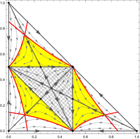
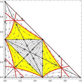
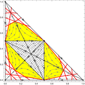
$d=1$	$d=2$	$d=3$
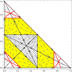
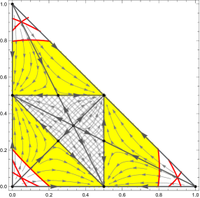
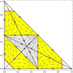
$d=4$	$d=5$	$d=6$

Figure 3. Phase portrait of the Projected Ricci flow is depicted jointly with the regions $\operatorname{\mathcal{R}^{\mathrm{\,Ric-scal}}_{d}}$ (see Definition 6). The yellow regions represent the metrics $g\in\operatorname{\mathcal{R}^{\mathrm{\,sec-Ric}}_{d}}$ that lose this property under the Ricci flow. Meanwhile, the checkered inner triangle represents the metrics $g\in\operatorname{\mathcal{R}^{\mathrm{\,Ric-scal}}_{d}}$ for which the projected Ricci flow $g(t)$ with $g(0)=g$ satisfies $g(t)\in\operatorname{\mathcal{R}^{\mathrm{\,Ric-scal}}_{d}}$ for all $t\in\mathbb{R}$.

5. Associated bundles and intermediate positive curvatures

This section follows the procedure systematically described in [CGS22], which consists, in nature, of a metric deformation on fiber bundles with a compact structure group.

Let $F\hookrightarrow M\stackrel{{\scriptstyle\pi}}{{\to}}B$ be a fiber bundle from a compact manifold $M$, with compact fiber $F$ and compact structure group $G$. We denote the base manifold by $B$. Given a lie group $G$, if it acts effectively on $F$, then $G$ is a structure group for $\pi$ if some choice of local trivializations takes values on $G$. Any fiber bundle recovers a principal $G$-bundle over $B$ (see [KN69, Proposition 5.2] for details), which we denote by $P$. It is straightforward checking that the following is a $G$-bundle, $\overline{\pi}:P\times F\to M$, whose principal action is given by

(22) $$r(p,f):=(rp,rf).$$

(See, for instance, the construction on the proof of [GW09, Proposition 2.7.1].)

For each pair g and $\textsl{g}_{F}$ of $G$-invariant metrics on $P$ and $F$, respectively, there exists a metric h on $M$ induced by $\overline{\pi}$. Fixing a point $(p,f)\in P\times F$, any vector $\overline{X}\in T_{(p,f)}(P\times F)$ can be written as $\overline{X}=(X+V^{\vee},X_{F}+W^{*})$, where $X$ is orthogonal to the $G$-orbit on $P$, $X_{F}$ is orthogonal to the $G$-orbit on $F$ and, for $V,W\in\mathfrak{g}$, $V^{\vee}$ and $W^{\ast}$ are the action vectors relative to the $G$-actions on $P$ and $F$ respectively, see for instance [CGS22, Section 2] for further clarifications.

Chosen a bi-invariant metric $Q$ on $G$ and Riemannian metrics $\textsl{g},~{}\textsl{g}_{F}$, it comes from the fact that two any Riemannian metrics are pointwise related by a symmetric tensor the existence of almost everywhere pointwise positive-definite symmetric tensors $O,~{}O_{F}$, named the orbit tensors associated to $\textsl{g},~{}\textsl{g}_{F}$, that codify the geometry of the orbits of $G$ on $P$ and $F$, comparing g with $Q$ and $\textsl{g}_{F}$ with $Q$, to know

$$\textsl{g}_{F}(U^{*},V^{*})=Q(O_{F}U,V),\ \textsl{g}(U^{\vee},V^{\vee})=Q(OU,V).$$

It is worth pointing recalling that the almost everywhere positive definiteness is justified as: If $G$-acts effectively on a smooth manifold $F$, it exists an open and dense subset $F^{reg}\subset F$ such that every two points have conjugate isotropy subgroups. Furthermore, for any $G$-invariant metric $\textsl{g}_{F}$ on $F$, the induced metric in $F^{reg}/G$ is named the orbit distance metric. For points $f\in F\setminus F^{reg}$, the orbit tensor $O_{F}$ may lose rank. This is explored in Lemma 3.

It comes from [CGS22, Section 3.1] that any $\overline{X}$ is $\textsl{g}+\textsl{g}_{F}$-orthogonal to the $G$-orbit of (22) if and only if

(23) $$\overline{X}=(X-(O^{-1}O_{F}W)^{\vee},X_{F}+W^{\ast}).$$

for some $W\in\mathfrak{g}$. Fixing $(p,f)$, we may abuse the notation and denote

(24) $$d\bar{\pi}_{(p,f)}(X,X_{F}+U^{*}):=X+X_{F}+U^{*}.$$

It can be proved [CGS22, Theorem 3.1]:

Theorem 5.1 (Sectional curvature under a fiber bundle Cheeger deformation).

Let $\textsl{h}_{t}$ be a Riemannian submersion metric in $M$ obtained from the product metric $\textsl{g}_{t}+\textsl{g}_{F}$, where $\textsl{g}_{t}$ is a Cheeger deformation of g. Then for every pair $\tilde{X}=X+X_{F}+U^{*}$, $\tilde{Y}=Y+Y_{F}+V^{*}$ ,

$$\tilde{\kappa}_{\textsl{h}_{t}}(\tilde{X},\tilde{Y})=\kappa_{\textsl{g}_{t}}(X{+}U^{\vee},Y{+}V^{\vee}){+}K_{\textsl{g}_{F}}(X_{F}-(O_{F}^{-1}OU)^{*},Y_{F}-(O_{F}^{-1}OV)^{*})+\tilde{z}_{t}(\tilde{X},\tilde{Y}),$$

where $\kappa_{\textsl{g}_{t}}$ is the unreduced sectional curvature of $\textsl{g}_{t}$ computed on some appropriate reparameterization of a two-plane $X{+}U^{\vee}\wedge Y{+}V^{\vee}$ of $TP$ and $\tilde{z}_{t}$ is non-decreasing in $t$.

It is possible to adapt the proof of Lemmas 5 and 7 in [CGS22] to obtain

Lemma 1.

Fix a point $(p,f)\in P\times F$ such that the $G$-orbit at $f$ is principal and $X+X_{F}+U^{*}\in T_{\bar{\pi}(p,f)}M$. Choose a non-negative integer $1\leq d\leq 5$. Made a choice of non-negative integers $n_{\mathcal{H}_{f}^{F}},n_{\mathfrak{m}_{f}}$ constrained by the dimensions of $F$ and its $G$-orbits and satisfying $d=n_{\mathcal{H}_{f}^{F}}+n_{\mathfrak{m}_{f}}$, we have

(25) $$\lim_{t\to\infty}\operatorname{Ric}_{d,\textsl{h}_{t}}(X+X_{F}+U^{*})=\operatorname{Ric}_{n_{B},\textsl{g}_{B}}(d\pi X)+\operatorname{Ric}^{\mathbf{h}}_{n_{\mathcal{H}_{f}^{F}}}(X_{F})+\sum_{j=1}^{n_{\mathcal{H}_{f}^{F}}}\frac{3}{4}|[X,e^{F}_{j}]^{\mathfrak{m}_{f}}|_{g_{F}}^{2}+\sum_{k=1}^{n_{\mathfrak{m}_{f}}}\frac{1}{4}\|[v_{k}(0),U]\|_{Q}^{2}.$$

Remark 2.

The detailed description of each term appearing in equation (25) is given in the proof of the next proposition.

We can now prove the first part of the thesis in Theorem C, Proposition 5.2 below.

Proposition 5.2.

Let $F\rightarrow M\rightarrow\mathrm{SU}(3)/\mathrm{T}^{2}$ as in the hypotheses of Theorem C. Then for any choice of invariant metric $\textsl{g}_{B}$ on $B=\mathrm{SU}(3)/\mathrm{T}^{2}$ with positive sectional curvature, after choosing a Riemannian metric on $F$ appropriately, we can regard the total space $M$ with a Riemannian submersion metric of positive $\operatorname{Ric}_{d_{F}+1}$.

Proof.

Once Lemma 1 is in hand, we approach the proof by contradiction, relying on the analysis in purely combinatorial aspects.

Observe that each of the terms in equation (25) are non-negative except, maybe, for $\operatorname{Ric}_{n_{B},\textsl{g}_{B}}(d\pi X)+\operatorname{Ric}_{n_{\mathcal{H}_{f}^{F}}}^{\mathbf{h}}(X_{F})$. In this manner, one must impose the needed constraints on such terms. Let us assume that $\textsl{g}_{B}$ has positive sectional curvature. We recall that $\mathrm{SU}(3)/\mathrm{T}^{2}$ always admits one of such a metric; see Theorem A.

Given any $G$-invariant Riemannian metric $\textsl{g}_{F}$ such that $\operatorname{Ric}_{F^{reg}/G,d_{F}}>0$ on $F^{reg}/G$, $d_{F}\geq 1$, we regard $M$ with the Riemannian submersion metric $\textsl{h}_{1}=\textsl{h}$ which is a Riemannian connection metric for which fibers $F$ are totally geodesic, obtained exactly as in the Proposition 2.7.1 in [GW09].

Now observe that for each $f\in F$, we have that $T_{f}F\cong\mathfrak{m}_{f}\oplus\mathcal{H}_{f}^{F}$, where $\mathfrak{m}_{f}\subset\mathfrak{\mathrm{missing}}{su}(3)$ is isomorphic with the tangent space to the $\mathrm{SU}(3)$-orbit $\mathrm{SU}(3)f$ and $\mathcal{H}^{F}_{f}:=(T_{f}\mathrm{SU}(3)f)^{\perp_{\textsl{g}_{F}}}$. Hence, any basis for $T_{f}F$ has $\dim\mathfrak{m}_{f}+\dim\mathcal{H}_{f}^{F}$ elements, which we denote by $\{v_{1}(0),\ldots,v_{\dim\mathfrak{m}_{f}}(0)\}\cup\{e_{1}^{F},\ldots,e_{\dim\mathcal{H}_{f}^{F}}^{F}\}$. Therefore, when picking $d=d_{F}{+}1$ vectors out of a basis for $T_{p}M$, one has $d=d_{F}{+}1=n_{B}+n_{\mathfrak{m}_{f}}+n_{\mathcal{H}_{f}^{F}}$ where $0\leq n_{B}\leq 6=\dim\mathrm{SU}(3)/\mathrm{T}^{2},~{}0\leq n_{\mathfrak{m}_{f}}+n_{\mathcal{H}_{f}^{F}}\leq\dim F\leq 8=\dim\mathrm{SU}(3)$ and $n_{B}$ is the number of elements in this $d_{F}+1$-cardinality set which belongs to elements of the horizontal lifting $\mathcal{L}_{\bar{\pi}}T_{b}\mathrm{SU}(3)/\mathrm{T}^{2}$, $n_{\mathfrak{m}_{f}}$ the number of such elements which belong to $\mathfrak{m}_{f}$ and $n_{\mathcal{H}_{f}^{F}}$ the number of elements which belongs to $\mathcal{H}^{F}_{p}$.

Suppose a point $p\in M$ exists with orthonormal vectors $X\perp X_{F}+U^{*}$ satisfying

(26) $$\operatorname{Ric}_{h_{\infty},d}(X+X_{F}+U^{*})\leq 0$$

where the former is the abuse notation for $\lim_{t\to\infty}\operatorname{Ric}_{h_{t,d}}(X+X_{F}+U^{*})\leq 0$. Then, $\operatorname{Ric}_{n_{B},\textsl{g}_{B}}(X)+\operatorname{Ric}_{n_{\mathcal{H}_{f}^{F}}}^{\mathbf{h}}(X_{F})\leq 0$.

If $n_{B}\neq 0$ then $\operatorname{Ric}_{n_{B},\textsl{g}_{B}}(X)>0$ (since $\textsl{g}_{B}$ has positive sectional curvature) and so $\operatorname{Ric}_{n_{\mathcal{H}_{f}^{F}}}^{\mathbf{h}}(X_{F})<0$. Hence, since $\operatorname{Ric}_{F^{reg}/G,d_{F}}>0$, we have that either $1\leq n_{\mathcal{H}_{f}^{F}}<d_{F}$ or $f\in F\setminus F^{reg}$, that is, $f$ does not lie in a principal orbit, since for points in a principal orbit we have

$$\operatorname{Ric}_{F^{reg}/G,n_{\mathcal{H}^{F}}}(X_{F})=\operatorname{Ric}_{\textsl{g}_{F},n_{\mathcal{H}^{F}_{f}}}^{\mathbf{h}}(X_{F}){+}\sum_{j=1}^{n_{\mathcal{H}_{f}^{F}}}\frac{3}{4}|[X,e^{F}_{j}]^{\mathfrak{m}_{f}}|_{g_{F}}^{2}$$

and the former is positive if $X_{F}\neq 0$ and $n_{\mathcal{H}_{f}^{F}}\geq d_{F}$.

Now observe that the quantity below

$$\sum_{j=1}^{n_{\mathcal{H}_{f}^{F}}}\frac{3}{4}|[X,e^{F}_{j}]^{\mathfrak{m}_{f}}|_{g_{F}}^{2}+\sum_{k=1}^{n_{\mathfrak{m}_{f}}}\frac{1}{4}\|[v_{k}(0),U]\|_{Q}^{2}=\operatorname{Ric}_{n_{\mathfrak{m}_{f}}+n_{\mathcal{H}_{f}^{F}},\mathrm{SU}(3)f}(X_{F}+U^{*})$$

is precisely the $(n_{\mathfrak{m}_{f}}+n_{\mathcal{H}_{f}^{F}})\mathrm{th}$-Ricci curvature of the orbit $\mathrm{SU}(3)f$ in the normal homogeneous metric, with $n_{\mathfrak{m}_{f}}+n_{\mathcal{H}_{f}^{F}}\geq 1$, where $Q$ is any bi-invariant metric on $\mathrm{SU}(3)$. Moreover, $n_{\mathfrak{m}_{f}}=0$ since under our assumption, such curvature is positive for any $n_{\mathfrak{m}_{f}}\geq 1$, see Lemma 2 below. In any case, since $\textsl{g}_{B}$ has positive sectional curvature, up to re-scaling this metric since $\operatorname{Ric}_{n_{B},\textsl{g}_{B}}(X)>0$, inequality (26) cannot hold. Therefore, $f\in F\setminus F^{reg}$.

However, this can not also hold since, up to switch $\textsl{g}_{F}$ to a finite Cheeger deformation of it (Lemma 3), inequality (26) could not hold as well. Therefore, $n_{B}=0$ and $f\in F^{reg}$. Moreover, $n_{\mathcal{H}_{f}^{F}}+n_{\mathfrak{m}_{f}}=d_{F}{+}1$ and inequality (26) is translated in

(27) $$\operatorname{Ric}_{F^{reg}/G,n_{\mathcal{H}^{F}}}(X_{F})+\sum_{k=1}^{n_{\mathfrak{m}_{f}}}\frac{1}{4}\|[v_{k}(0),U]\|_{Q}^{2}\leq 0,$$

that is precisely $\lim_{t\to\infty}\operatorname{Ric}_{d_{F}+1,(\textsl{g}_{F}),t}(X_{F}{+}U^{*})$, i.e., the $(d_{F}+1)$-Ricci curvature of the limit as $t\to\infty$ of a Cheeger deformation $(\textsl{g}_{F})_{t}$ of $\textsl{g}_{F}$, see Lemmas 2.6 and 4.2 in [CeSS23]. Since $d_{F}{+1}\geq 2$ Lemma 2 concludes the proof, once it yields a contradiction with inequality (27):

$$\operatorname{Ric}^{\mathbf{h}}_{\textsl{g}_{F},n_{\mathcal{H}^{F}_{f}}}(X_{F})+\operatorname{Ric}_{n_{\mathfrak{m}_{f}}+n_{\mathcal{H}_{f}^{F}},\mathrm{SU}(3)f}(X_{F}+U^{*})\leq 0$$

but

$$\operatorname{Ric}_{n_{\mathfrak{m}_{f}}+n_{\mathcal{H}_{f}^{F}},\mathrm{SU}(3)f}(X_{F}+U^{*})>0$$

can be made arbitrarily large after a canonical variation, that is, scaling the metric $\textsl{g}_{F}$ along $\mathrm{SU}(3)f$, which does not change $\operatorname{Ric}^{\mathbf{h}}_{\textsl{g}_{F},n_{\mathcal{H}^{F}_{f}}}(X_{F})$. ∎

Lemma 2.

Assume that a principal orbit of the $\mathrm{SU}(3)$-action on $F$ has as isotropy subgroup a maximal closed subgroup. Then every non-principal orbit is a fixed point, that is, $\mathrm{SU}(3)f=f$ for $f\in F\setminus F^{reg}$. Moreover, for every point $f^{\prime}$ in a principal orbit (i.e., $f^{\prime}\in F^{reg})$, the homogeneous space $\mathrm{SU}(3)f^{\prime}$ has positive $\operatorname{Ric}_{2}$ at the normal homogeneous space metric.

Proof.

According to our hypothesis if $f$ lies in a principal orbit $\mathrm{SU}(3)f$ we have that

$$\mathrm{SU}(3)f\cong\mathrm{SU}(3)/H$$

where $H$ is a maximal proper closed subgroup of $\mathrm{SU}(3)$. According to [AFG12, Section 8.1, p. 1006] we have the following possibilities for $H$:

1. Type 1: normalizer of a maximal connected subgroup.

   $$\mathrm{U}(2)\cong\mathrm{S}(\mathrm{U}(2)\times\mathrm{U}(1))$$

   $$\zeta_{3}\times\mathrm{SO}(3)$$

2. Type 2: finite maximal closed subgroup.

   $$\zeta_{3}\times\mathrm{GL}(3,2)\equiv\zeta_{3}\times\mathrm{Gl}(3,\mathbb{F}_{2})$$

   $$3.\mathrm{A}_{6}$$

   $$\mathrm{S}(\mathrm{Cl}_{1}(3))$$

3. Type 3: normalizer of a positive dimensional non-maximal connected subgroup.

   $$\mathrm{S}(\mathrm{U}(1)\times\mathrm{U}(1)\times\mathrm{U}(1))\rtimes\mathrm{S}_{3}$$

where $\mathrm{S}(\mathrm{Cl}_{1}(3))$ is the determinant minus one subgroup of the single qutrit Clifford group, i.e., Shephard-Todd-25, [ST54]. The group $3.\mathrm{A}_{6}$ is known as the Valentiner group ([Val89]), and $\zeta_{3}$ is the short notation for the Lie group generated as $\langle\zeta_{3}I\rangle=\left\langle\begin{pmatrix}e^{2\pi k\mathbf{i}/3}&0\\ 0&e^{-2\pi k\mathbf{i}/3}\end{pmatrix}:k\in\{0,1,2\}\right\rangle$. As normal homogeneous spaces, we have the only possibilities for $\mathrm{SU}(3)/H$:

1. $\mathrm{SU}(3)/\mathrm{S}(\mathrm{U}(2)\times\mathrm{U}(1))\cong\mathrm{SU}(3)/\mathrm{U}(2)$;  $\mathrm{SU}(3)/\mathrm{SO}(3)$

2. $\mathrm{SU}(3)/H$ where its Riemannian covering is $\mathrm{SU}(3)$ via a finite ramified covering map (that is, with discrete fibers of finite cardinality)

3. $\mathrm{SU}(3)/\mathrm{T}^{2}$.

According to Proposition 3.1 in [DVGÁM22] we get that if $\mathfrak{su}(3)=\mathfrak{m}\oplus\mathfrak{h}$ is the standard reductive decomposition of $\mathrm{SU}(3)/H$ the minimum value of $d$ yielding positive $\operatorname{Ric}_{d,\mathrm{SU}(3)/H}$ at the normal homogeneous space metric is given by

$$\max_{x\in\mathfrak{m}\setminus\{0\}}\dim Z_{\mathfrak{m}}(x)$$

where $Z_{\mathfrak{m}}(x)=\{y\in\mathfrak{m}:[x,y]=0\}$. Remark 3.6 in [DVGÁM22] verifies the claim for the homogeneous spaces in (ii) observing that $\mathrm{SU}(3)$ admits $\operatorname{Ric}_{2}>0$; while Theorem A ensures the result for the homogeneous space in item (iii). Item (i) follows from the brackets computed in Table 1 with the definition of $Z_{\mathfrak{m}}(x)$.

Finally, for the claim on every non-principal orbit being a fixed point, observe that if $\mathrm{SU}(3)f\cong\mathrm{SU}(3)/\overline{H}$ is a non-principal orbit, it has different orbit type than a principal orbit, see [AB15, Section 3.5]. Suppose $H$ is a principal isotropy subgroup, i.e., $\mathrm{SU}(3)/H$ is a principal orbit. In that case, $H$ is conjugate to a closed subgroup of $\overline{H}<\mathrm{SU}(3)$, what contradicts $H$ being a closed maximal subgroup of $G$ unless $\overline{H}=\mathrm{SU}(3)$. ∎

Remark 3.

According to Theorem D in [DVGÁM22], or as compiled in Table 3 in the same reference, some of the homogeneous spaces described in Lemma 2 do not admit metrics with $\operatorname{Ric}_{2}>0$ when seen as a symmetric space. Observe, however, that our result does not contradict Proposition 3.8 in [DVGÁM22].

Lemma 3.

Let $F$ as in the hypotheses of Theorem C. Then for any $\mathrm{SU}(3)$-invariant Riemannian metric $\textsl{g}_{F}$ and every $f\in F\setminus F^{reg}$ there exists a non-zero vector $X_{F}+U^{*}\in T_{f}F$ such that $\operatorname{Ric}_{\textsl{g}_{F},d_{F}}(X_{F}+U^{*})$ is arbitrarily large for any $d_{F}\geq 2$ after a finite Cheeger deformation of $\textsl{g}_{F}$.

Sketch of the proof.

Since points belonging to non-principal orbits for the $\mathrm{SU}(3)$ are fixed points (Lemma 3), for each of such, we can always pick $X_{F}+U^{*},~{}Y_{F}+V^{*}\in T_{f}F$ such that the $z_{t}$-term in a Cheeger deformation (Lemma 3.5 in [CeSS23]) blows up as $t\nearrow+\infty$ when computed in such elements, as in Proposition 3.4 in [CeSS23]. We can conclude the claim by collapsing $F$ to a point in Theorem 5.1 since such a formula reduces to the ones usually employed in Cheeger deformations, such as Proposition 1.3 in [Zil]. Compare, for instance, with the proof of Theorem C in [CeSS23].∎

5.1. The proof of Theorem C

We finally prove Theorem C. We do this by combining the well-known quadratic trick, employed similarly in [CS22, Theorem 1.6], with a family of metrics obtained as in Proposition 5.2. To know, given any invariant positively curved Riemannian metric $\textsl{g}_{B}$ on $\mathrm{SU}(3)/\mathrm{T}^{2}$, we consider on $M$ the metric with totally geodesic fibers given by Proposition 2.7.1 in [GW09], assuming that the $\mathrm{SU}(3)$-invariant metric on $F$ induces a Riemannian metric in $F^{reg}/\mathrm{SU}(3)$ that has positive $\operatorname{Ric}_{d_{F}}$. We can do more indeed; consider a curve of Riemannian metrics $\textsl{g}_{B}(t)$ in $B=\mathrm{SU}(3)/\mathrm{T}^{2}$ as solutions of the projected homogeneous Ricci flow with initial condition $\textsl{g}_{B}(t=0)=\textsl{g}_{B}$ and employ Proposition 2.7.1 in [GW09] to build a family of connection metrics $\textsl{g}(t)$ on $M$ fixing an initial choice of Riemannian metric $\textsl{g}_{F}$ on the fiber.

Following Theorem 1.6 in [CS22], we performed a $s$-canonical variation of $\textsl{g}_{t}$, namely, we make $\textsl{g}_{t}\Big{|}_{\mathcal{H}\times\mathcal{H}}+e^{2s}\textsl{g}_{t}\Big{|}_{\mathcal{V}\times\mathcal{V}}=(\textsl{g}_{t})_{s}:=\textsl{g}_{t,s}$, and show that: There is $t>0$ such that for any $s<0$ arbitrarily small, there is a unit vector $\widetilde{X}=X+X_{F}+U^{*}$ for $X\perp X_{F}+U^{*}$ satisfying $\operatorname{Ric}_{d_{F}+1}(\widetilde{X})\leq 0$.

As a first step, observe that Proposition 5.2 ensures that for any $0\leq t\ll 1$, we have that g has positive $\operatorname{Ric}_{d_{F}+1}$. To conclude our goal, take $\lambda\in\mathbb{R}$ and assume that $X,X_{F}+U^{*}$ are mutually orthonormal. We expand the polynomial $p_{t,s}(\lambda)=\operatorname{Ric}_{\textsl{g}_{t,s}}(X+\lambda(X_{F}+U^{*}))$, which is 2-degree in $\lambda$. We show that there is $t>0$ such that for any $s<0$ arbitrarily small, the discriminant of $p_{t,s}$ is non-positive for some $X\perp X_{F}+U^{*}$ with $\|X\|=\|X_{F}+U^{*}\|=1$.

Take $t^{*}>0$ defined by $t^{*}:=\inf\{t\geq 0:\exists X\in T^{1}\mathrm{SU}(3)/\mathrm{T}^{2}:\operatorname{Ric}_{\textsl{g}_{B}(t),1}(X)\leq 0\}$, which exists, see for instance Figure 2. We show that for any $t>t^{*}$, no $s<0$ arbitrarily small preserves the positivity of $\operatorname{Ric}_{d_{F}+1}$. Indeed, the limit $s\rightarrow-\infty$ leads to the following discriminant of $p_{t,s}(\lambda)$ (see the proof of Theorem 1.6 in [CS22])

$$\Delta_{t,-\infty,\lambda}=\operatorname{Ric}_{n_{B},t}(X)\operatorname{Ric}_{n_{F},\textsl{g}_{F}}(X_{F}+U^{*}),$$

where $n_{F}+n_{B}=d_{F}$. Since $t>t^{*}$, pick $n_{B}=1$ and $X$ such that $\operatorname{Ric}_{1,t}(X)=0$. We have that $\Delta_{t,-\infty,\lambda}=0$ and $p_{t,-\infty}(\lambda)=\operatorname{Ric}_{n_{B},t}(X)+\lambda^{2}\operatorname{Ric}_{n_{F},\textsl{g}_{F}}(X_{F}+U^{*})$, taking $\lambda=0$ finishes the proof.

References

[AB15]
M. M. Alexandrino and R. G. Bettiol.
Lie Groups and Geometric Aspects of Isometric Actions.
Springer International Publishing, 2015.
[AFG12]
F. Antoneli, M. Forger, and P. Gaviria.
Maximal Subgroups of Compact Lie Groups.
Journal of Lie Theory, 22(4):949–1024, 2012.
[AL19]
Romina M. Arroyo and Ramiro A. Lafuente.
The long-time behavior of the homogeneous pluriclosed flow.
Proc. Lond. Math. Soc. (3), 119(1):266–289, 2019.
[AN16]
Nurlan Abievich Abiev and Yuriĭ Gennadievich Nikonorov.
The evolution of positively curved invariant Riemannian metrics on
the Wallach spaces under the Ricci flow.
Annals of Global Analysis and Geometry, 50(1):65–84, Jul 2016.
[Bes87]
A. Besse.
Einstein manifolds, Springer.
1987.
[BFF20]
Leonardo Bagaglini, Marisa Fernández, and Anna Fino.
Laplacian coflow on the 7-dimensional Heisenberg group.
Asian J. Math., 24(2):331–354, 2020.
[BL19]
Christoph Böhm and Ramiro A. Lafuente.
The Ricci flow on solvmanifolds of real type.
Adv. Math., 352:516–540, 2019.
[BLP22]
Renato G. Bettiol, Emilio A. Lauret, and Paolo Piccione.
Full Laplace spectrum of distance spheres in symmetric spaces of
rank one.
Bulletin of the London Mathematical Society, 54(5):1683–1704,
2022.
[BW07]
Christoph Böhm and Burkhard Wilking.
Nonnegatively curved manifolds with finite fundamental groups admit
metrics with positive Ricci curvature.
Geom. Funct. Anal., 17(3):665–681, 2007.
[BWZ]
C. Böhm, M. Wang, and W. Ziller.
A variational approach for compact homogeneous Einstein manifolds.
Geom. Funct. Anal., 14:681–733.
[CeSS23]
Leonardo F. Cavenaghi, Renato J. M. e Silva, and Llohann D. Sperança.
Positive Ricci curvature through cheeger deformations.
Collectanea Mathematica, Feb 2023.
[CGM23]
Leonardo F. Cavenaghi, Lino Grama, and Ricardo M. Martins.
On the dynamics of positively curved metrics on
under the homogeneous ricci flow.
arXiv eprint 2305.06119, 2023.
[CGS22]
Leonardo F. Cavenaghi, Lino Grama, and Llohann D. Sperança.
The concept of Cheeger deformations on fiber bundles with compact
structure group.
São Paulo Journal of Mathematical Sciences, Nov 2022.
[Che73]
J. Cheeger.
Some examples of manifolds of nonnegative curvature.
J. Diff. Geom., 8:623–628, 1973.
[CS22]
Leonardo Francisco Cavenaghi and Llohann Dallagnol Sperança.
Positive Ricci curvature on fiber bundles with compact structure
group.
Advances in Geometry, 22(1):95–104, 2022.
[CW12]
Man-Wai Cheung and Nolan Wallach.
Ricci flow and curvature on the variety of flags on the two
dimensional projective space over the complexes, quaternions and octonions.
Proceedings of the American Mathematical Society, 143, 06 2012.
[CW20]
Diarmuid Crowley and David Wraith.
Intermediate curvatures and highly connected manifolds.
arXiv eprint 1704.07057, 2020.
[DVGÁM22]
Miguel Domínguez-Vázquez, David González-Álvaro, and Lawrence
Mouillé.
Infinite families of manifolds of positive -th intermediate
Ricci curvature with small.
Mathematische Annalen, Aug 2022.
[FR21]
Anna Fino and Alberto Raffero.
A class of eternal solutions to the -Laplacian flow.
J. Geom. Anal., 31(5):4641–4660, 2021.
[GAZ23]
David González-Álvaro and Masoumeh Zarei.
Positive intermediate curvatures and Ricci flow.
arXiv eprint 2303.08641, 2023.
[GMPa+22]
L. Grama, R. M. Martins, M. Patrão, L. Seco, and L. Sperança.
The projected homogeneous Ricci flow and its collapses with an
application to flag manifolds.
Monatsh. Math., 199(3):483–510, 2022.
[GW09]
D. Gromoll and G. Walshap.
Metric Foliations and Curvature.
Birkhäuser Verlag, Basel, 2009.
[KM23]
Lee Kennard and Lawrence Mouillé.
Positive intermediate Ricci curvature with maximal symmetry rank.
arXiv eprint 2303.00776, 2023.
[KN69]
S. Kobayashi and K. Nomizu.
Foundations of Differential Geometry.
Number v. 1 in Interscience tracts in pure and applied mathematics.
Interscience, 1969.
[Lau17]
Jorge Lauret.
Laplacian flow of homogeneous -structures and its solitons.
Proc. Lond. Math. Soc. (3), 114(3):527–560, 2017.
[LPV20]
Ramiro A. Lafuente, Mattia Pujia, and Luigi Vezzoni.
Hermitian curvature flow on unimodular Lie groups and static
invariant metrics.
Trans. Amer. Math. Soc., 373(6):3967–3993, 2020.
[Mou]
Lawrence Mouillé.
Intermediate Ricci curvature.
Website
https://sites.google.com/site/lgmouille/research/intermediate-ricci-curvature.
[Mou22]
Lawrence Mouillé.
Local symmetry rank bound for positive intermediate Ricci
curvatures.
Geometriae Dedicata, 216(2):23, Mar 2022.
[RW22a]
Philipp Reiser and David J. Wraith.
Intermediate Ricci curvatures and Gromov’s Betti number bound.
arXiv eprint 2208.13438, 2022.
[RW22b]
Philipp Reiser and David J. Wraith.
Positive intermediate Ricci curvature on fibre bundles.
arXiv eprint 2211.14610, 2022.
[SM21]
Luiz A.B. San Martin.
Lie Groups.
Springer International Publishing, 2021.
[ST54]
G. C. Shephard and J. A. Todd.
Finite unitary reflection groups.
Canadian Journal of Mathematics, 6:274–304, 1954.
[SW15]
C. Searle and F. Wilhelm.
How to lift positive Ricci curvature.
Geometry & Topology, 19(3):1409–1475, 2015.
[Val89]
H. Valentiner.
De endelige Transformations-Gruppers Theori, volume 2.
Bianco Lunos Bogtrykkeri, Jun 1889.
[WZ]
M. Wang and W. Ziller.
Existence and non-existence of homogeneous einstein metrics.
Invent. Math., 84.
[Zil]
W. Ziller.
On M. Müter’s PhD thesis.
https://www.math.upenn.edu/ wziller/papers/SummaryMueter.pdf.