The Photon Sphere and the AdS/CFT Correspondence

Abstract

By rephrasing the radial Klein–Gordon equation for a scalar field on anti-de Sitter (AdS) Schwarzschild black hole background in terms of an auxiliary field that satisfies a Schrödinger equation, we demonstrate that the properties of the photon sphere play an important role in the AdS/CFT correspondence. Most importantly, we use constraints imposed by the UV cutoff to derive a highly precise formula describing how a black hole in the bulk amplifies or attenuates an oscillating source dual to boundary operators across the bulk. This formula leads us to identify a phase transition that traps massless fields, which correspond to scalar sources for dual boundary operators, outside the photon sphere when their angular momenta are large enough for classical particles with a matching impact parameter to travel between boundary points. We then use similar reasoning to determine an approximate analytic formula for the QNMs of small black holes at large $l$. The condition for a signal/source to pierce the potential barrier peaking at the photon sphere is, roughly, that its frequency must be greater than the angular momentum of its driven operator times the square of the Lyapunov exponent of the unstable null geodesics.

1 Introduction

For many first-time learners of general relativity, the photon sphere, originally examined in Bardeen:1972fi as marginally trapped light rays, may appear as a seemingly inconsequential peculiarity associated with black holes, as commonly presented in textbooks such as Misner:1973prb ; hartle2003gravity . However, it is important to note that photon spheres actually play a significant role in various aspects of astrophysics and gravitational physics, demonstrating their profound importance in understanding the properties and behavior of black holes. They have recently gained significant attention for two compelling reasons. Firstly, on the more theoretical side, they play a crucial role in imaging Einstein rings of black holes in Anti-de Sitter (AdS) spacetime Hashimoto:2018okj ; Hashimoto:2019jmw , in the emergence of conformal symmetries associated to enhanced bright regions (“photon (sub)rings”) from gravitaional lensing by a Kerr black hole in asymptotically flat spacetime Johnson:2019ljv ; Gralla:2019drh ; Himwich:2020msm ; Hadar:2022xag , and in other theoretical implications such as warped AdS₃ black holes Kapec:2022dvc . Secondly, the practical application of imaging astrophysical black hole shadows, such as those of M87* EventHorizonTelescope:2019dse and Sgr A* EventHorizonTelescope:2022wkp by the Event Horizon Telescope, has sparked renewed interest in the study of photon spheres. An extensive review on analytical techniques for calculating black hole photon rings and shadows can be found in PERLICK20221 .

In addition to photon spheres, another key player in the study of black holes is the concept of quasi-normal modes (QNMs). For scalar fields, QNMs are roughly defined as solutions to the Klein–Gordon equation (28) that are purely out-going near infinity ($\Phi\sim e^{-i\omega(t-r_{*})}$) and purely in-going near the black hole horizon ($\Phi\sim e^{-i\omega(t+r_{*})}$). Only a discrete set of complex frequencies $\omega$ is allowed due to the absence of physical meaning of initial incoming waves from infinity. In asymptotically AdS spacetimes, the effective potential (see Appendix B) vanishes exponentially near the horizon and diverges at infinity, requiring $\Phi(r)$ to vanish at infinity. Complex frequencies determine the late-time fall-off of fields $\Phi(r)$.

Albeit just being solutions to linear second-order ODEs, QNMs offer a powerful approach for understanding the behavior of perturbations around black holes Berti:2009kk . Various techniques have been developed to solve for QNMs over the past few decades. The WKB method, along with its variant called the monodromy method for highly damped modes, has proven effective in many types of spacetimes, particularly asymptotically flat ones Schutz:1985km ; Iyer:1986np ; Iyer:1986nq . Frobenius series solutions are well-suited for asymptotically AdS spacetimes, while a resonance method has shown better results for small black holes. The use of continued fractions, first introduced by Leaver Leaver:1985ax ; leaver1986solutions ; Leaver:1986gd , has also been applied to asymptotically AdS spacetimes recently Daghigh:2022uws . Other methods include Regge poles Decanini:2009dn and purely numerical techniques. Numerous investigations of QNMs have been subsequently conducted, as summarized in the comprehensive review by Berti et al. Berti:2009kk . Several important aspects contribute to the understanding of QNMs. The retarded Green’s function and the fact that they do not form a complete set of basis Berti:2009kk are fundamental in their calculations. The computation involves an inverse Laplace transform, whose contour integral on the complex frequency plane includes contributions from two quarter-circles, a branch cut responsible for late-time long tails, and a sum over residues.

Early studies of black holes in asymptotically AdS spacetime were conducted by Horowitz and Hubeny in Horowitz:1999jd among others, revealing important properties such as QNM frequencies (both their real and complex parts) are proportional to the temperatures of large black holes. Notably, contrary to QNMs for the black holes in asymptotically flat spacetimes, where Price:1972pw revealed the existence of power-law tails, those of AdS-Schwarzschild black holes do not exhibit such tails as shown by Ching:1994bd ; Ching:1995tj . Power-law behavior in the intermediate time regime of QNMs is absent in AdS-Schwarzschild as well Horowitz:1999jd .

Moreover, QNMs has further deepened the understanding of AdS/CMT (condensed matter theory) correspondence hartnoll2018holographic , because they are natural physical quantities in the dual strongly coupled field theory without weakly interacting quasiparticle excitations. Specifically, when going beyond scalar operators $\mathcal{O}$ to current operators $J^{\mu}$, QNMs also describe the charge transport in the quantum critical theory. Moreover, functional determinant or partition function for semiclassical gravity in both asymptotically AdS and dS can be expressed as a product over QNMs Denef:2009kn ; Keeler:2014hba ; Keeler:2016wko , offering $1/N$ corrections, such as the singular long-time tail in the electrical conductivity at the one-loop level Kovtun:2003vj . Other related applications of QNMs include determining the viscosity-to-entropy-density ratio in hyperscaling-violating Lifshitz theories Mukherjee:2017ynv , as well as studying strange metals Andrade:2018gqk , hydrodynamic transports Policastro:2002tn ; Herzog:2003ke ; Kovtun:2005ev , operator mixings Kaminski:2009dh , and phase transitions in superfluids and superconductors Amado:2009ts ; Bhaseen:2012gg .

It should be noted that the relationship between QNMs and the size of black hole photon spheres (or shadows) is not simply expressed in terms of the impact parameter in AdS spacetimes, as discussed in PERLICK20221 and Cardoso:2008bp . This intricacy adds to the subtlety of the physical connections between QNMs and photon spheres in AdS spacetime. Moreover, recent research by Bardeen Bardeen:2018omt has highlighted the predominant generation of Hawking radiation near the photon sphere of a black hole in asymptotically flat spacetime. This finding has further emphasized the importance of understanding the relationship between QNMs and photon spheres. Further motivated by the intriguing way of detecting the existence of a gravitational dual of a given $3$d boundary theory using the temperature-dependence of $4$d planar AdS-Schwarzschild black hole images Hashimoto:2018okj ; Hashimoto:2019jmw , we delve deeper into the precise relationship between photon spheres and QNMs here.

We exclusively work with massless fields $\Phi(t,r,\theta,\phi)$ in the AdS₄-Schwarzschild background, satisfying the Klein–Gordon equation. In the light of AdS/CFT correspondence, its conformal dimension dictates its asymptotic behavior near the AdS boundary – its corresponding oscillating source ($\propto e^{i\omega t}$) and the expectation value of its dual operator can be read off from the leading and subleading terms, respectively. When solving the Klein–Gordon equation, we obtain a Helmholtz-like equation for radial modes $\phi_{l}(r)$ labeled by angular momenta, saying that for large $l$, $\phi_{l}(r)$ are pushed away from the origin, where the effective potential takes its maximum value.

The effective potential takes its local maximum values at two places – at the AdS boundary, and at the photon sphere. The solutions to the Klein–Gordon equation are well-approximated by null geodesics in the WKB limit, so we expect the field to be confined between the AdS boundary and the photon sphere for high enough angular momentum $l$. Since the scalar field is related to the source and the expectation value of the operator it sources, we suggest the AdS/CFT correspondence could depend in an interesting way on the angular momentum of the dual operator.

By exploring an interesting connection between the Klein–Gordon equation and the Schrodinger equation, we then derive a formula that describes the amplification of fields as they propagate from the UV cutoff to the horizon of the black hole (51). Using the WKB approximation and a field redefinition, the formula has a physical interpretation as a tunneling process. The derivation then follows from the cutoff invariance of the theory. For black holes of the order of the Hawking–Page transition and above, the formula gives an excellent approximation for the amplitude of a field at the horizon of the black hole when the eikonal approximation is valid. We then explain the breakdown of this approximation in terms of massless particles orbiting the photon sphere many times in the vicinity of their critical impact parameter. Finally, we use similar reasoning to determine the QNMs of small (below the Hawking–Page temperature) AdS black holes in the large angular momentum limit.

The rest of the paper is organized as follows. In Section 2, we review the notion of photon sphere in AdS spacetime in the context of classical particles, set up notations and coordinate systems, and describe the behavior of massless particles traveling along null geodesics in terms of an impact parameter. In Section 3 we set up an analogous problem for the Klein–Gordon equation. In Section 4, we derive the amplification formula (51), which determines the fate – amplifying or decaying – of a signal incident from the asymptotic boundary as it approaches an AdS black hole. It also predicts two phase transitions in accordance with the geodesic approximation in the eikonal limit. In Section 5, we compute the Lyapunov exponent, which turns out to equal the critical value of the impact parameter. We then determine the QNMs of an AdS black hole, well below the Hawking–Page transition, at high angular momentum $l$. We obtain a closed-form analytical solution which depends on the Lyapunov exponent, but we obtain the modes using an approximation method outlined in Cardoso:2008bp . In Section 6, we present our numerical results in the context of the amplification formula and speculate on the meaning of our findings. We conclude in Section 7, leaving the full investigation on the large-angular-momentum sector in the dual CFT inspired by the photon sphere to later, among other future directions. We collected various technical details on solving ODEs and a review on WKB approximation to Appendices A and B. Finally, Appendix C contains many visualizations of the amplification formula (51).

2 The Photon Sphere

This section is an overview of known properties of the photon sphere, generalizing them to the AdS case when necessary. The photon sphere is already known to play a key role in determining the spectrum of QNMs in asymptotically flat spacetimes Cardoso:2008bp ; Decanini:2009dn . Still, an extension to asymptotic anti-de Sitter spacetimes has proved challenging. Owing to its status as an important astrophysical object, for example, in gravitational wave astronomy and accretion disks, there are many useful reviews of its properties PERLICK20221 ; Berti:2009kk .

2.1 Conserved Quantitites and the Impact Parameter

This discussion parallels a useful review PERLICK20221 that presents how the photon sphere of a four-dimensional spherically symmetric black hole determines its shadow, a concept originally described in Bardeen:1972fi . These arguments apply to spherically symmetric and static metrics, which can be placed in the form:

$$g_{\mu\nu}dx^{\mu}dx^{\nu}=-A(r)dt^{2}+B(r)dr^{2}+D(r)\left(d\vartheta^{2}+\sin^{2}\vartheta d\varphi^{2}\right),$$ (1)

with $A(r),B(r),D(r)>0$. We aim to understand the amount of angular momentum a massless particle needs in order to travel between two points on the AdS boundary. The first step is to phrase the Lagrangian $\mathcal{L}(x,\dot{x})=(1/2)g_{\mu\nu}\dot{x}^{\mu}\dot{x}^{\nu}$ in a particularly useful form which eliminates the square root:

$$\mathcal{L}(x,\dot{x})=\frac{1}{2}\left(-A(r)\dot{t}^{2}+B(r)\dot{r}^{2}+D(r)\left(\dot{\vartheta}^{2}+\sin^{2}\vartheta\dot{\varphi}^{2}\right)\right).$$ (2)

Since this system has an axial symmetry, we can choose a convenient angle to work with – i.e., we choose $\vartheta=\frac{\pi}{2}$, on the equitorial plane. Since the Lagrangian now does not depend on $\vartheta$ or $t$, the equations of motion

$$\frac{d}{d\lambda}\left(\frac{\partial\mathcal{L}}{\partial\dot{x}^{\mu}}\right)-\frac{\partial\mathcal{L}}{\partial x^{\mu}}=0,$$ (3)

yield the energy ($\omega$) and angular momentum ($l$) as conserved quantities:

$$\omega=A(r)\dot{t},\quad l=D(r)\dot{\varphi}.$$ (4)

The ratio of these conserved quantities is usually called the “impact parameter”:

$$b:=\frac{\omega}{l},$$ (5)

which plays an important role in determining the fate of a particle emitted from the asymptotic boundary. Its effects can be conveniently summarized using an effective potential to be introduced.

2.2 The Effective Potential and the Impact Parameter

The standard procedure to proceed is clearly outlined in PERLICK20221 . For a massless particle, it is customary to study the first integral of its geodesic equation, which turns out to be:

$$-A(r)\dot{t}^{2}+B(r)\dot{r}^{2}+D(r)\dot{\varphi}^{2}=0.$$ (6)

Rewriting this in terms of the conserved quantities in Equation (4), and then solving for $\frac{\dot{r}^{2}}{\dot{\varphi}^{2}}=\left(\frac{dr}{d\varphi}\right)^{2}$ gives:

$$\left(\frac{dr}{d\varphi}\right)^{2}=\frac{D(r)}{B(r)}\left(\frac{D(r)}{A(r)}\frac{\omega^{2}}{l^{2}}-1\right).$$ (7)

The expression in Equation (7) clearly depends only on the coefficients in the metric, $A(r)$, $B(r)$, and $D(r)$, and on the ratio $b$ (5) of the conserved quantities $\omega$ and $l$.

This equation essentially takes the form of an oscillator where the effective potential is the RHS of Equation (7). In cases where a geodesic launched from the boundary of AdS returns to the boundary, there will be a turning point in the trajectory at some radial location $R_{t}$. Here $dr/d\phi=0$, so we obtain a relationship between $R_{t}$ and the impact parameter $b$ :

$$\frac{\omega^{2}}{l^{2}}=b^{2}=\frac{A(R_{t})}{D(R_{t})}.$$ (8)

It is convenient to introduce a function called the effective potential:

$$h(r):=\frac{A(r)}{D(r)},$$ (9)

which implies that the turning point is related to the impact parameter as

$$b^{2}=h(R_{t}).$$ (10)

The equations of motion can then be written as:

$$\left(\frac{dr}{d\varphi}\right)^{2}=\frac{D(r)}{B(r)}\left(\frac{h(r)}{h(R_{t})}-1\right).$$ (11)

We now partly specialize to a Schwarzschild black hole by taking $A(r)=\frac{1}{B(r)}$:

$$g_{\mu\nu}dx^{\mu}dx^{\nu}=-A(r)dt^{2}+\frac{1}{A(r)}dr^{2}+D(r)\left(d\vartheta^{2}+\sin^{2}\vartheta d\varphi^{2}\right).$$ (12)

Using Equation (7) and Equation (10), we obtain an expression that can be used to determine the classical turning points for the motion:

$$\left(\frac{dr}{d\varphi}\right)^{2}=\frac{D(r)}{B(r)}\left(\frac{D(r)}{A(r)}\frac{\omega^{2}}{l^{2}}-1\right) =D(r)^{2}\left(\frac{\omega^{2}}{l^{2}}-\frac{A(r)}{D(r)}\right)$$ (13)

$$=D(r)^{2}\left(b^{2}-h(r)\right).$$

Massless particles traveling along geodesics at position $R$ travel toward (away) from the boundary depending on how their effective potential compares to their impact parameter. Regardless of where they originate – whether deep in the bulk, or at the asymptotic boundary – if they can reach that point, they will turn around at radial position $h(R_{t})=b^{2}$.

2.3 The Photon Sphere and Geodesic Orbits in AdS-Schwarzschild

Now we specialize to an AdS-Schwarzschild black hole in asymptotically AdS_d spacetime, whose metric is:

$$g_{\mu\nu}dx^{\mu}dx^{\nu}=-F(r)dt^{2}+\frac{1}{F(r)}dr^{2}+r^{2}d\Omega_{d-2}.$$ (14)

Then using Equation (6), the blackening function, $F(r)$, the effective potential $h(r)$ (9), and the equations of motion (13) are

$$F(r) =1+\frac{r^{2}}{L^{2}}-\frac{2M}{r^{d-3}},$$ (15)

$$h(r) =\frac{F(r)}{r^{2}},$$

$$\left(\frac{dr}{d\varphi}\right)^{2}=r^{2}\left(b^{2}-\frac{F(r)}{r^{2}}\right).$$ (16)

The behavior of the effective potential is illustrated in Figure 1. It is interesting to consider the orbits of the null geodesics. The boundary conditions are given by initializing $r=r_{0}$ and then determining the momentum from (16):

$$p=\frac{dr}{d\tau}=\left(\frac{dr}{d\varphi}\right)\left(\frac{d\varphi}{d\tau}\right)=\sqrt{\left(\omega^{2}-\frac{l^{2}F(r)}{r^{2}}\right)}.$$ (17)

One then solves (16) to obtain the null geodesics, which were computed in Mathematica for AdS spacetime and illustrated in Figure 2. There is an unstable point where massless particles can travel around the black hole; their trajectories form a geometric object known as the photon sphere. Its radius $r_{ps}$ corresponds to the unstable maximum value of the effective potential:

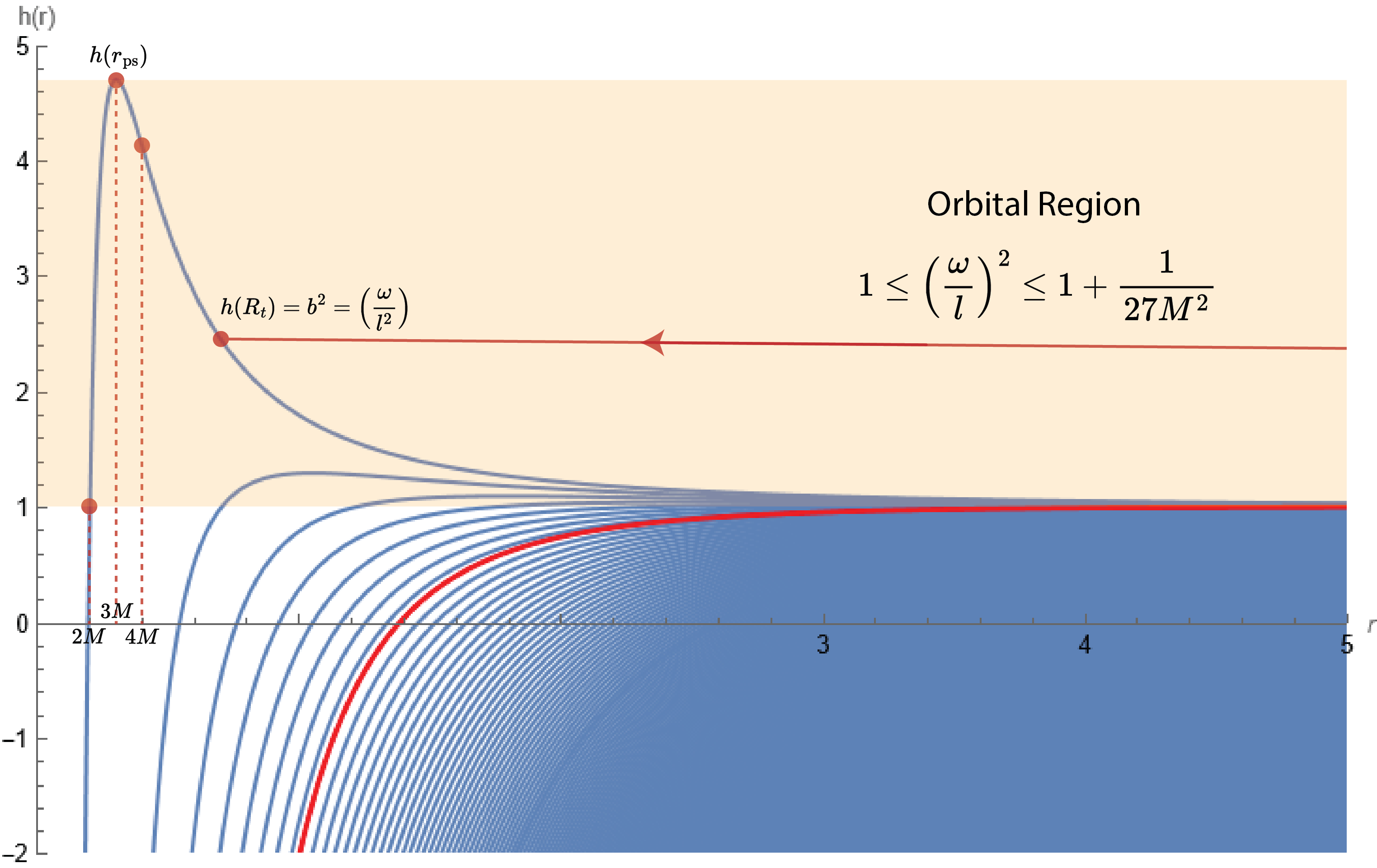
Figure 1: Here we show the effective potential, $h(r)=F(r)/r^{2}$, for a massless particle near an asymptotically AdS-Schwarzschild black hole for a large range of black hole masses $M\in(0.1,200)$. The effective potential decreases monotonically with $M$. For a particle to leave the AdS boundary and travel between boundary points without falling into the black hole, its impact parameter must lie within $h(2M)<b^{2}<h(3M)$, corresponding to the shaded region for $M=0.1$. The red line corresponds to the Hawking–Page transition that occurs when the radius $R$ of the black hole becomes smaller than the AdS radius $L$. The effective potential has a clear maximum (at the photon sphere) that becomes difficult to see above the Hawking–Page transition. The photon sphere approaches the event horizon as the black hole becomes small, and approaches the AdS boundary as the black hole becomes large. Note that the effective potential is shifted vertically upward, compared to the asymptotically flat case.

Figure 2: Here we show the geodesic trajectories for massless particles in an AdS spacetime. The photon sphere is pictured as the dark ring around the horizon in black. Their behavior can be predicted from their impact parameters alone from Equation (25). Panel $1$ shows an inspiral trajectory because the value of its impact parameter is greater than the critical value at the photon sphere, i.e., $b>1+1/27M^{2}$. The other three panels show scattering trajectories. Particles with impact parameters $b<1$ cannot leave the asymptotic boundary and are not pictured. One can obtain a scattering (or inspiral) trajectory that orbits the photon sphere arbitrarily many times before returning to the boundary (or falling into the black hole) by choosing an impact parameter sufficiently close to the critical value. We find that the solutions to the scalar wave equation (36) behave similarly; modes corresponding to sources of frequency $\omega$, which drive operators of angular momentum $l$, penetrate the photon sphere only when their “impact parameter” satisfies essentially the same condition (51). Moreover, the solutions are unstable, sharply peak at the photon sphere, and violate (51) when $b$ is sufficiently close to the critical value. See Figures 4-6.

$$h^{\prime}(r_{\text{ps}})=0.$$ (18)

This gives the radial position of the photon sphere as:

$$r_{\text{ps}}=\left(\frac{1}{(d-1)M}\right)^{\frac{1}{3-d}}.$$ (19)

It is interesting to note that the mass of the black hole suffices to determine the location of the photon sphere. This is because the effective potential can be written as:

$$h(r)=\frac{1}{r^{2}}+\frac{k}{L^{2}}-\frac{2M}{r^{d-1}},$$ (20)

where $k=0,1,-1$ for asymptotically flat, AdS, and dS spacetimes, respectively. From here on, we choose $L=1$ for convenience and specialize to $d=4$. Since the second term depending on the geometry does not explicitly depend on $r$, the equation for the photon sphere (18) in terms of the mass is the same in all three types of spacetime. As in asymptotically flat space, when we choose $d=4$ the location of the photon sphere is:

$$r_{\text{ps}}=3M.$$ (21)

The effective potential is related to its counterpart in flat space by:

$$h(r)-k=h_{\text{flat}}(r).$$ (22)

Since $k$ does not depend on $r$, it follows immediately that the $n$-th derivative of $h(r)$ with $n\geq 1$ satisfies

$$h^{(n)}(r)\bigg{|}_{r=(2+n)M}=0.$$ (23)

For example, as a consequence of Equation (23), the photon sphere occurs at $r=3M$ and the maximum acceleration of the particle occurs at $r=4M$.

For asymptotic AdS spacetime, the effective potential on the boundary is $h(\infty)=1/L^{2}=1$, so massless particles cannot leave the boundary without satisfying $b>1$. For them to return to the boundary, their impact parameter cannot exceed the maximum value of the effective potential, which is given by its value at the location of the photon sphere:

$$h(r_{\text{ps}})=1+\frac{1}{27M^{2}}.$$ (24)

We conclude that, for the geodesic to travel between two points on the boundary, its impact parameter $b=\omega/l$ must lie in the range:

$$1\leq\frac{\omega^{2}}{l^{2}}\leq 1+\frac{1}{27M^{2}}:=b_{\text{crit}}^{2},$$ (25)

namely

$$h(2M)<b^{2}<h(3M).$$ (26)

It is worth briefly considering the limit where the black hole becomes large ($M\rightarrow\infty$), known as the planar limit. In that case, the impact parameter must equal the reciprocal of the AdS radius. Furthermore, the effective potential becomes:

$$h_{\text{planar}}(r)=\frac{1}{r^{2}}-\frac{2M}{r},$$ (27)

which does not have a photon sphere. It can be seen from Equations (24), (25), and (26) that the photon sphere approaches the boundary as $M\rightarrow\infty$, and that the impact parameter for geodesics traveling between boundary points becomes confined in an increasingly narrow range. The photon sphere moves toward the event horizon when we take the limit where the black hole becomes small $(M\rightarrow 0)$. In this limit, the potential increasingly resembles the asymptotically flat case, but even in the limit as $M\rightarrow 0$, the potential is still shifted up by $1$.

3 The Scalar Wave Equation on a Schwarzschild Background

Here we motivate our findings by exploring the well-known analogy, in the eikonal limit, between the wave equation for a minimally-coupled massless scalar field $\Phi(t,r,\theta,\phi)$ on an AdS₄-Schwarzschild background and the equation of motion for a null geodesic. The field must satisfy the Klein–Gordon equation:

$$g_{\mu\nu}\nabla^{\mu}\nabla^{\nu}\Phi(t,r,\theta,\phi)=0.$$ (28)

Specializing to a Schwarzschild black hole with blackening function $F(r)$, this yields:

$$\frac{1}{F}\partial_{t}^{2}\Phi+F\partial^{2}_{r}\Phi+\frac{\partial_{r}(r^{2}F)}{r^{2}}\partial_{r}\Phi+\frac{\nabla^{2}}{r^{2}}\Phi=0,$$ (29)

where $\nabla^{2}$ is the scalar Laplacian on $S^{d-2}$. Since this problem has an azimuthal symmetry, we can solve this equation by expanding its solution in spherical harmonics $Y_{lm}$ with $m=0$:

$$\Phi(t,r,\theta,\phi)=e^{-i\omega t}\sum_{l}c_{l}\phi_{l}(r)Y_{l\,0}(\theta).$$ (30)

This approach is useful due to the property:

$$\nabla^{2}Y_{lm}(\theta,\phi)=\frac{-l(l+1)}{r^{2}}Y_{lm}(\theta,\phi).$$ (31)

This leads to the differential equation for the radial field with angular momentum $l$:

$$F(r)^{2}\phi_{l}^{\prime\prime}(r)+\left(\frac{2F(r)^{2}}{r}+F(r)F^{\prime}(r)\right)\phi_{l}^{\prime}(r)+\left(\omega^{2}-\frac{l(l+1)F(r)}{r^{2}}\right)\phi_{l}(r)=0.$$ (32)

3.1 Tortoise Coordinates and Schrödinger Form

The equations of motion (32) simplify in tortoise coordinates:

$$r_{*}:=\int\frac{1}{F(r)}dr\Leftrightarrow\frac{d}{dr_{*}}:=F(r)\frac{d}{dr},$$ (33)

because:

$$\left(\frac{d}{dr_{*}}\right)\phi_{l}(r_{*}) =F(r)\phi_{l}^{\prime}(r),$$ (34)

$$\left(\frac{d}{dr_{*}}\right)^{2}\phi_{l}(r_{*}) =F(r)F^{\prime}(r)\phi_{l}^{\prime}(r)+F(r)^{2}\phi_{l}^{\prime\prime}(r).$$ (35)

It is straightforward to use the above equations to show that:

$$\left(\frac{d}{dr_{*}}\right)^{2}\phi_{l}(r_{*})+\left(\frac{2F(r)}{r}\right)\left(\frac{d}{dr_{*}}\right)\phi_{l}(r_{*})+\left(\omega^{2}-\frac{l(l+1)F(r)}{r^{2}}\right)\phi_{l}(r_{*})=0,$$ (36)

where the blackening function $F(r)$ is evaluated in the original $r$-coordinates. Now conveniently, this equation resembles the radial Helmholtz equation, which takes the following form for a radial field $R(r)$:

$$\left(\frac{d}{dr}\right)^{2}R(r)+\frac{2}{r}\left(\frac{d}{dr}\right)R(r)+\left(k^{2}-\frac{l(l+1)}{r^{2}}\right)R(r)=0.$$ (37)

This has an effective potential term $1/r^{2}$, and the term proportional to $l(l+1)$ is known as the “centrifugal” term. This gives a potential barrier that pushes solutions radially outward away from the origin, where the effective potential achieves its diverging global maximum. From this we can draw some intuition for the effect of the centrifugal term in Equation (36) – the effective potential is now $F(r)/r^{2}$ as in Equation (15), and the centrifugal term pushes solutions outward away from the photon sphere, which is the local maximum for the effective potential. For these reasons, we anticipate that solutions $\phi_{l}(r_{*})$ corresponding to a source on the boundary will be found outside the photon sphere for large $l$.

To convert Equation (36) to the Schrödinger form, we make use of the field redefinition described in Appendix A to obtain:

$$\left(\frac{d}{dr_{*}}\right)^{2}\psi_{l}(r_{*})+\left(\omega^{2}-\underbrace{\frac{l(l+1)F(r)}{r^{2}}-\frac{F(r)F^{\prime}(r)}{r}}_{V(r)}\right)\psi_{l}(r_{*})=0,$$ (38)

where $\psi_{l}(r):=r\phi_{l}(r)$, and where we have specialized to $d=4$. There Klein–Gordon equation in Schrödinger form clearly resembles the equation for the geodesics of massless particles (7). The multiplicative coefficient of $\psi_{l}(r_{*})$ in Equation (38) is positive when:

$$\frac{\omega^{2}}{l(l+1)}>\frac{F(r)}{r^{2}}+\frac{F^{\prime}(r)F(r)}{rl(l+1)}.$$ (39)

In the limit where the angular momentum, $l$, becomes large, we obtain:

$$\frac{\omega^{2}}{l(l+1)}>\frac{F(r)}{r^{2}}=h(r),$$ (40)

which is roughly the same as the condition for null geodesics to travel between boundary points in Equation (25). We will make this much more concrete in Section 4. Since $\psi$ takes the form of the Schrödinger equation, we will analyze its behavior by using the semi-classical WKB approximation – i.e., the wave must tunnel through a potential with a local maximum at the photon sphere. The second term, $F^{\prime}(r)F(r)/r$, acts as a “reflective” potential barrier located on the boundary:

$$\frac{F^{\prime}(r)F(r)}{r}=\frac{r^{-2d-1}\left(L^{2}+r^{2}\right)\left(Rr^{d}-rR^{d}\right)\left((d-1)R^{d}\left(L^{2}+r^{2}\right)+2Rr^{d+1}\right)}{L^{4}R^{2}}.$$ (41)

In asymptotically flat spacetimes, $L\rightarrow\infty$ yields $F^{\prime}(r)F(r)/r\rightarrow 0$ at the boundary. But for asymptotically AdS_d spacetimes, it is simple to show that this diverges as $F(r)F^{\prime}(r)/r\sim 2r^{2}/L^{4}$, which gives basically an infinite potential barrier at the boundary. Nonetheless, once a UV cutoff is imposed, one might hope this term would drop out for sufficiently large $l$. It turns out it does, as shown in the next section.

4 An Amplification Formula for Sources

According to the AdS/CFT correspondence, the sources and expectation values of operators in the boundary CFT can be obtained by first solving the classical wave equation in the bulk and then performing an asymptotic expansion near the boundary to determine the leading and subleading terms in the field. In this note, we exclusively focus on massless scalar fields in the bulk, corresponding to certain scalar operators in the boundary CFT. We anticipate that our argument would go through mostly unchanged for Maxwell and gravitational fields, but we leave that intriguing prospect for future work.

4.1 Brief Review of the AdS/CFT Correspondence

First, we briefly review the AdS/CFT correspondence and specialize to our case. For a scalar field of mass $m$ the conformal dimension $\Delta$ in an AdS_d bulk can be determined from:

$$\Delta(\Delta-d+1)=m^{2}.$$ (42)

In our case $d=4$ and $m=0$, so we have:

$$\Delta_{-}=0,\quad\Delta_{+}=3.$$ (43)

According to the AdS/CFT dictionary, the field $\Phi$ near the asymptotic boundary expanded in terms of $1/r$ can be written as Klebanov:1999tb ; Hashimoto:2018okj :

$$\Phi(t,r,\theta,\phi)=J_{\mathcal{O}}(t,\theta,\phi)-\frac{1}{2r^{2}}\left(\partial_{t}^{2}-\nabla^{2}\right)J_{\mathcal{O}}(t,\theta,\phi)+\frac{\expectationvalue{\mathcal{O}(t,\theta,\phi)}}{r^{3}}+\dots,$$ (44)

where $J_{\mathcal{O}}$ is the oscillating source (with frequency $\omega$) for the scalar operator $\mathcal{O}$ dual to $\Phi$ in the boundary CFT, so that $J_{\mathcal{O}}$ and the expectation value of $\mathcal{O}$ can be read off from the asymptotic expansion. The source is the boundary value of the field at the UV cutoff, while the response function $\expectationvalue{\mathcal{O}}$ corresponds to the coefficient of the $1/r^{3}$ term.

4.2 An Amplification Formula

Here we derive an interesting formula for the sources $J_{\mathcal{O}}$, with frequency $\omega$, that drive operators $\mathcal{O}$ with angular momentum $l$ on the boundary CFT dual to the AdS-Schwarzschild bulk. Note that, like massless particles traveling along null geodesics, we are free to define an impact parameter for the pair $(J_{\mathcal{O}}(\omega),\mathcal{O}_{l})$:

$$b^{2}:=\left(\frac{\omega}{l}\right)^{2}.$$ (45)

Recall that massless bulk particles will fall into the black hole unless they have sufficient angular momentum to travel between boundary points (25). According to an observer on the boundary, their energy is amplified as if they fall into the black hole. Furthermore, they cannot leave the AdS boundary unless they have $\omega>l$, and if their impact parameter $b=\omega/l$ lies between the bounds of (25) they cannot fall into the black hole. Now we argue that bulk fields corresponding to sources $J_{\mathcal{O}}$ obey the same rule, with $\omega$ – the energy of the particle – exchanged for the frequency of the source, and $l$ – its angular momentum – exchanged for the angular momentum of the boundary operator.

Recall the two equivalent definitions for the equations of motion for the massless scalar field – these are Equations (36) and (38), where $\psi=r\phi$. The amplification formula follows from first using the WKB approximation on the “Schrödinger” form of the $\psi$ field and then obtaining the $\phi_{l}$ field from $\psi_{l}=r\phi_{l}$. After carefully treating the UV cutoff, this leads to a constraint that determines the formula.

Suppose the angular momentum $l$ of the operator with a source of frequency $\omega$ is large enough that the eikonal condition applies. Then according to the WKB approximation, as reviewed in Appendix B, far away from the classical turning points the wavefunction $\psi_{l}(r_{*})$ is approximately:

$$\psi_{l}(r_{*})\approx\frac{1}{\sqrt{\absolutevalue{p(r_{*})}}}e^{i\int p(r_{*})dr_{*}},$$ (46)

where $p(r)=\sqrt{\omega^{2}-V(r)}$ is the “classical momentum”, with $V(r)$ given by Equations (87) and (38). When $l$ is sufficiently large, the “reflective” term at the AdS boundary drops out of the region of interest, and the geodesic condition (25) essentially determines whether $p(x)$ is real or imaginary – when it is satisfied, $p(x)$ is real, and there will be no potential barriers for the wavefunction $\psi_{l}(r_{*})$ to tunnel through into the region of interest. The effective potential is, therefore, reasonably well approximated by its maximum value:

$$\frac{F(r)}{r^{2}}\approx 1+\frac{1}{27M^{2}}.$$ (47)

Later we will show that this value is also the square of the Lyapunov exponent. Then by the WKB approximation (46), the solution $\psi_{l}(r_{*})$ to Equation (38) is well approximated by a field with a constant amplitude:

$$|\psi_{l}(r_{*})|\approx\frac{1}{\sqrt{\omega^{2}-l(l+1)\left(1+\frac{1}{27M^{2}}\right)}}.$$ (48)

Now that we have used the WKB approximation on the “Schrödinger” equation, we can obtain $\phi_{l}$ by taking advantage of $r\phi_{l}=\psi_{l}$. Since the constant amplitude of $\psi(r_{*})$ is well approximated by Equation (48) everywhere in the region of interest, we cannot freely choose the cutoff to be anything we like – indeed, $r\phi_{l}=\psi_{l}$, and this means we have no choice but to choose the cutoff to make the amplitude of $\psi_{l}$ satisfy Equation (48). Without loss of generality, we can assume we normalize the boundary value of $\phi_{l}$ to $1$. Since the tortoise coordinates at the boundary equals $r_{*}=1/r$, we must choose the following UV cutoff:

$$\epsilon=\frac{1}{\sqrt{\omega^{2}-l(l+1)\left(1+\frac{1}{27M^{2}}\right)}}.$$ (49)

Note that the inverse tortoise coordinate at the horizon equals the black hole radius $R$, and near the boundary $B$, the tortoise coordinate is given by $r_{*}(r_{B})=1/r=\epsilon$. Remarkably, our choice of the UV cutoff allows the tortoise coordinate to produce $\phi_{l}$ from $\psi_{l}$, which has a constant amplitude, even though the tortoise coordinate should not know the angular momentum $l$. Calling the horizon $H$:

$$R\,\phi_{l,H}=r(r_{*,H})\phi_{l,H}=\psi_{l,H}=\psi_{l,B}=\frac{\phi_{l,B}}{r_{*}(r_{B})}=\frac{\phi_{l,B}}{\epsilon}.$$ (50)

The amplification formula then follows:

$$\frac{\phi_{l,B}}{\phi_{l,H}}=\frac{R}{\sqrt{\omega^{2}-l(l+1)\left(1+\frac{1}{27M^{2}}\right)}}.$$ (51)

It is roughly true that when the geodesic condition (25) is unsatisfied, it also follows that $p(r_{*})<0$, and $\psi_{l}(r_{*})$ will rapidly decay as it propagates through the broad peak in the potential barrier at the photon sphere. Hence, the following equation gives an approximate condition for the vanishing of $\psi_{l,H}$:

$$\lambda^{2}:=1+\frac{1}{27M^{2}}>\frac{\omega^{2}}{l(l+1)},$$ (52)

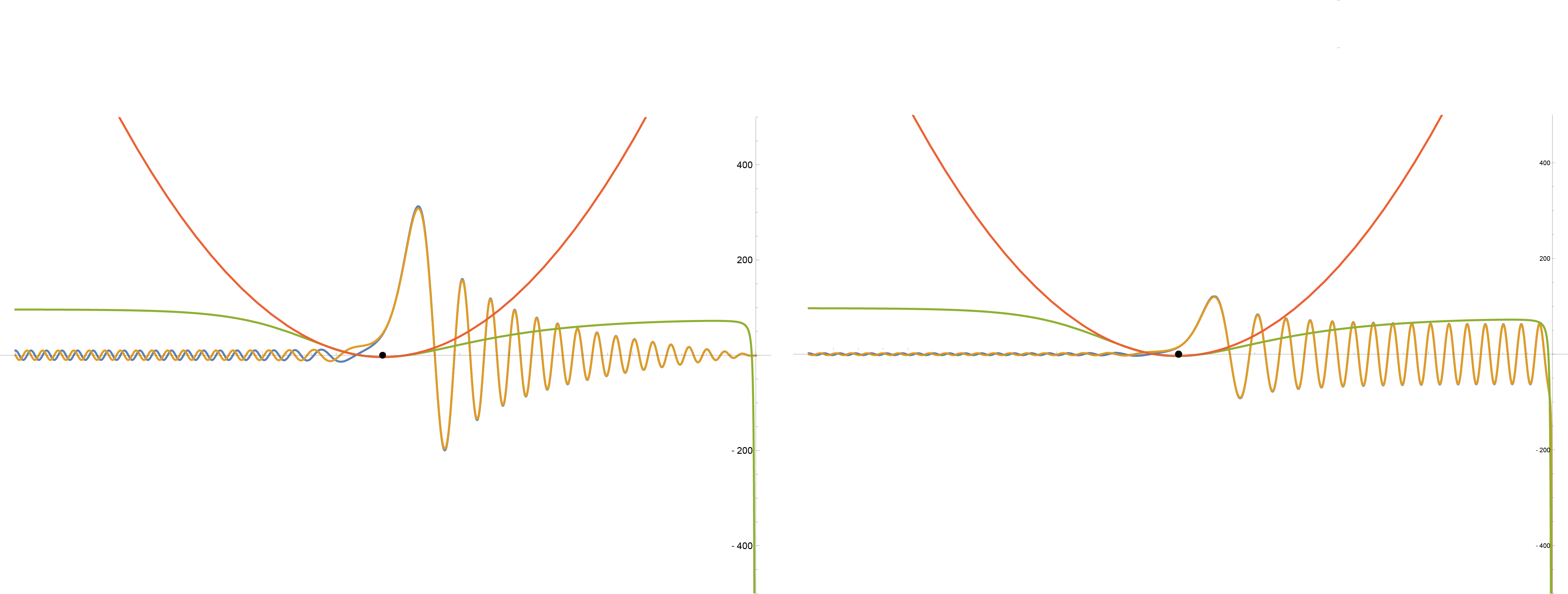
Figure 7: Here we present the phenomenon of the vanishing of scalar fields with frequency $\omega$ inside the photon sphere, for sufficiently large angular momentum $l$, as a tunneling effect from the perspective of the auxiliary radial field $\psi=r\phi$ in tortoise coordinates. The field $\phi$, which lives in an AdS-Schwarzschild background, is holographically dual to a scalar operator of angular momentum $l$ living in the $3$d CFT. The green curve is $p(x)^{2}=\omega^{2}-V(x)$, which predicts the decay of the field in the WKB approximation, and the red curve is the approximated $p(x)$ using the Lyapunov exponent (59).

where $\lambda$ is the Lyapunov exponent to be defined in the next section. The reader should note the clear resemblance to Equation (25). We will now point out some of the limitations of our argument. First of all, the frequency $\omega$ of the source and the mass $M$ of the black hole must be sufficiently large – if $M$ is small enough, $V(r)$ will become sharply peaked at the photon sphere, as shown in Figure 3. One might think that as $M$ becomes large, since the photon sphere will move toward the AdS boundary, this could interfere with our argument regarding the cutoff. Nonetheless, as we will explain in Section 6, the approximation is quite accurate. This phenomenon was demonstrated numerically and can be seen in Figures 4-7 collected in Appendix C.

The amplification formula suggests an interesting relationship between the angular momentum of an operator and the region that its dual bulk fields probe. It could be that sources for boundary operators of angular momentum $l$, with frequency $\omega$, are somehow preferentially dual to bulk fields that probe the region far from the horizon when their impact parameter forbids a classical particle from falling into the AdS-Schwarzschild black hole. Bulk fields probing the region near the horizon could similarly relate to sources for boundary operators with small angular momentum $l$. Nonetheless, to speculate further, bulk fields that probe the photon sphere’s interior could still be holographically dual to sources that drive operators with large $l$ on the boundary, provided their frequency $\omega$ is high enough.

The concrete upshot of our computation is that sources are amplified or weakened through a simple formula (52) analogous to (25), and according to the frequency of a source and the angular momentum of its operator. Bulk fields that satisfy (51) cannot penetrate more than a short distance beyond the photon sphere. It may be possible to turn this argument around to gain insight into QNMs in AdS spacetime, which correspond to fluctuations with a vanishing source term. It is widely believed that the “ringdown” of QNMs for a perturbed black hole in the bulk encodes the approach to thermal equilibrium for the dual CFT on its AdS boundary Horowitz:1999jd . The next section shows a strong local maximum for small black holes that peaks at precisely $r_{*}=-\pi/2$ as $M\rightarrow 0$. We also find that, in the limit as $l$ becomes large, the effective potential for $\psi$ at the boundary becomes a vertical wall – this may permit a QNM analysis for small black holes where $V(r)$ resembles a potential well.

While black holes of the order of the Hawking–Page phase transition still feature a vertical wall in their effective potential for large $l$, the photon sphere in tortoise coordinates essentially overlaps with the boundary. This has the effect of washing out the “well” in the effective potential, even for large angular momentum quantum number $l$. It would be interesting to see if analyzing this potential well could provide insight into the Hawking–Page phase transition. In the next section, we take cautious first steps towards this process by analyzing the effective potential and determining the Lyapunov exponent for AdS-Schwarzschild black holes. We then obtain an approximation for $V(r)$ and attempt to determine the QNMs for black holes well below the Hawking–Page transition in AdS.

5 The Lyapunov Exponent, the Effective Potential, and QNMs

5.1 The Lyapunov Exponent

The Lyapunov exponent for QNMs in asymptotically flat backgrounds was determined in Cardoso:2008bp , and it plays a fundamental role in determining the QNMs of perturbed black holes in asymptotically flat spacetime:

$$\lambda=\frac{1}{\sqrt{2}}\sqrt{-\frac{r_{\text{ps}}^{2}}{F(r_{\text{ps}})}\left(\frac{d^{2}}{dr_{*}^{2}}\frac{F(r)}{r^{2}}\right)\bigg{|}_{r=r_{\text{ps}}}}\,.$$ (53)

As a first step towards determining the QNMs in AdS for large angular momentum $l$, we point out that a Taylor series around the local maximum of the effective potential – at the photon sphere – reduces to an inverted harmonic oscillator which depends on the Lyapunov exponent.

Provided that $l$ is large enough, the main contribution to the effective potential in the region of interest comes from the centrifugal term proportional to $l(l+1)$ in (38). Since $h^{\prime}(r_{\text{ps}})=0$, its Taylor series is:

$$\frac{V(r_{*})}{l(l+1)} =h(r_{\text{ps}})+\frac{1}{2}\left(\frac{d}{dr_{*}}\right)^{2}h(r)\bigg{|}_{r_{\text{ps}}}(r_{*}-r_{\text{ps}})^{2}$$ (54)

$$=h(r_{\text{ps}})\left(1-\lambda^{2}(r_{*}-r_{\text{ps}})^{2}\right).$$ (55)

This is an inverted harmonic oscillator potential, a potential barrier for the wavefunction $\psi_{l}$ to cross. From the roots of the quadratic polynomial, the width of the inverted harmonic oscillator potential is

$$\delta=\frac{2}{\lambda},$$ (56)

which provides a useful estimate for the width of the actual potential barrier. For a sufficiently large angular momentum $l$, we can estimate the decay percentage of $\psi_{l}$ using the WKB approximation.

Neglecting the reflective term (41), which we suppose we can ignore when $l$ is large enough – see Figure 3 – we see that a field driven by a source of frequency $\omega$ can tunnel through the potential barrier if

$$\frac{\omega^{2}}{l(l+1)}<h(r_{\text{ps}})\left(1-\lambda^{2}(r-r_{\text{ps}})^{2}\right).$$ (57)

The next step is to compute the Lyapunov exponent:

$$\lambda^{2}=-\frac{1}{2}\frac{r_{\text{ps}}^{2}}{F(r_{\text{ps}})}\left(\frac{d^{2}}{dr_{*}^{2}}\frac{F(r)}{r^{2}}\right)\bigg{|}_{r=r_{\text{ps}}}=-\frac{1}{2}\left(\frac{1}{1+\frac{1}{27M^{2}}}\right)\left(F(r)\frac{d}{dr}\right)\left(F(r)\frac{d}{dr}\right)\left(\frac{F(r)}{r^{2}}\right)\bigg{|}_{r=r_{\text{ps}}}.$$ (58)

Surprisingly, this yields the critical impact parameter (25):

$$\lambda^{2}=1+\frac{1}{27M^{2}}=h(r_{\text{ps}})=b_{\text{crit}}^{2}$$ (59)

We conclude that the Lyapunov exponent is the critical value of the impact parameter that distinguishes null geodesics that fall into the event horizon from those that do not. Furthermore, the width of the potential barrier follows from Equation (56):

$$\delta=\frac{2}{\sqrt{1+\frac{1}{27M^{2}}}}.$$ (60)

This estimation for the effective potential is highly accurate for large $l$, even near the asymptotic boundary. It turns out that the reflective term, $F(r)F^{\prime}(r)/r$, also features a small peak at the photon sphere, but this can be neglected for sufficiently large $l$. For the most part, the reflective term’s peak at the photon sphere matters only for black holes with very small masses. The effectiveness of our approximation is illustrated in Figure 3.

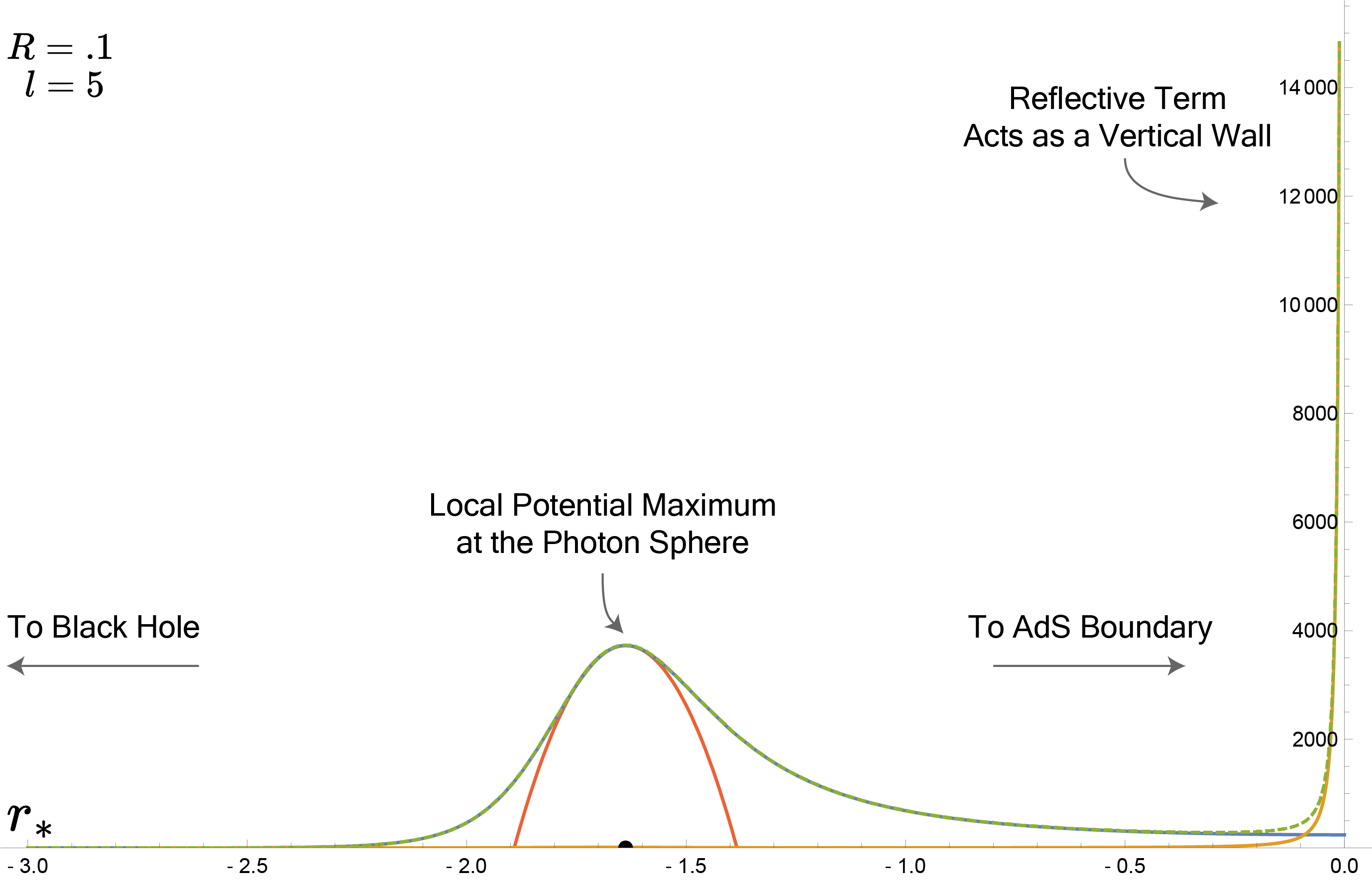
Figure 3: Here we show $V(r)$ for the auxiliary $\psi_{l}$ field in tortoise coordinates. The green curve is the actual value of the effective potential, the blue curve (which mostly overlaps with the green curve) is the centrifugal term $l(l+1)F(r)/r^{2}$, and the orange curve is the reflective term $F(r)F^{\prime}(r)/r$. As a general rule, the blue curve approximates the effective potential with high accuracy when $l$ is large. The red curve approximates the effective potential near the photon sphere in terms of the Lyapunov exponent (55). It is quite accurate for black holes smaller than the order of the Hawking–Page phase transition $(R=1)$. Since the “reflective” boundary potential is approximately a vertical wall, especially at large $l$, it should be possible to study this system using a WKB-style analysis. The photon sphere lies at approximately $r_{*}=-\pi/2$, as predicted by Equation (69).

5.2 The Lyapunov exponent and AdS-Schwarzschild Black Holes

The simple form of the Lyapunov exponent makes it possible to rephrase many key quantities in terms of it. We begin by solving for the mass of the black hole:

$$M=\frac{1}{\sqrt{27\lambda^{2}-27}}.$$ (61)

In Schwarzschild coordinates, we use the known equation for the mass in terms of the black hole radius $R$ to solve for the mass in terms of the Lyapunov exponent:

$$M=\frac{R(R^{2}+1)}{2},$$ (62)

so that

$$R=\frac{\sqrt[3]{\lambda+1}-\sqrt[3]{\lambda-1}}{\sqrt{3}\sqrt[6]{\lambda^{2}-1}}.$$ (63)

The Hawking–Page transition occurs when the radius of the black hole drops below the AdS radius – i.e., $R=1$. Equivalently, it occurs when $M=1$. Then the Hawking–Page transition, in terms of the Lyapunov exponent, takes place when:

$$\lambda=\sqrt{\frac{28}{27}}.$$ (64)

Meanwhile, the temperature of the Schwarzschild black hole is:

$$T=\frac{2}{F^{\prime}(r)}\bigg{|}_{r=R}=\frac{2R}{1+3R^{2}}=\frac{2\left(\sqrt[3]{\lambda+1}-\sqrt[3]{\lambda-1}\right)}{\sqrt{3}\sqrt[6]{\lambda^{2}-1}\left(\sqrt[3]{\frac{\lambda+1}{\lambda-1}}+\sqrt[3]{\frac{\lambda-1}{\lambda+1}}-1\right)}.$$ (65)

This achieves its maximum value at what is known as the spinodal point, which turns out to be related to the golden ratio $\phi$:

$$\lambda=\frac{\sqrt{5}}{2}=\phi-1/2.$$ (66)

It would be amusing to find out if this is related to the curious numerological fact that, for null geodesics with maximum radial acceleration in the de Sitter spacetime, the two classical turning points occur in the golden ratio Cruz:2017rbk .

With some effort, it is possible to compute an analytic formula for the location of the photon sphere in tortoise coordinates in terms of the Lyapunov exponent. Its location is:

$$P(\lambda):=r_{*,\text{ps}}=\frac{\sqrt[6]{\lambda+1}}{2\sqrt{6}\sqrt[6]{\lambda-1}}\bigg{[}A(\lambda)+B(\lambda)+C(\lambda)\bigg{]},$$ (67)

where functions $A(\lambda)$, $B(\lambda)$, and $C(\lambda)$ are:

$$A(\lambda) =-\frac{2\sqrt[3]{(\lambda-1)^{2}(\lambda+1)}\left(\sqrt[3]{\frac{\lambda-1}{\lambda+1}}-1\right)\log\left(\frac{\sqrt[3]{(\lambda-1)^{2}(\lambda+1)}-\sqrt[3]{(\lambda-1)(\lambda+1)^{2}}+1}{\sqrt{3}\sqrt{\lambda^{2}-1}}\right)}{-\sqrt[3]{(\lambda-1)^{2}(\lambda+1)}+\sqrt[3]{(\lambda-1)(\lambda+1)^{2}}+\lambda-1},$$ (68)

$$B(\lambda) =\frac{\left(\left(1+i\sqrt{3}\right)\sqrt[3]{\frac{\lambda-1}{\lambda+1}}+i\sqrt{3}-1\right)\log\left(\frac{1}{6}\left(\frac{\left(\sqrt{3}-3i\right)\sqrt[3]{\lambda+1}}{\sqrt[6]{\lambda^{2}-1}}-\frac{\sqrt{3}\left(1+i\sqrt{3}\right)\sqrt[6]{\lambda^{2}-1}}{\sqrt[3]{\lambda+1}}+\frac{2\sqrt{3}}{\sqrt{\lambda^{2}-1}}\right)\right)}{1-\frac{\left(-i\sqrt[3]{\frac{\lambda-1}{\lambda+1}}+\sqrt{3}\sqrt[3]{\frac{\lambda-1}{\lambda+1}}+i+\sqrt{3}\right)^{2}}{4\sqrt[3]{\frac{\lambda-1}{\lambda+1}}}},$$

$$C(\lambda) =\frac{\left(\left(1-i\sqrt{3}\right)\sqrt[3]{\frac{\lambda-1}{\lambda+1}}-i\sqrt{3}-1\right)\log\left(\frac{1}{6}\left(\frac{\left(\sqrt{3}+3i\right)\sqrt[3]{\lambda+1}}{\sqrt[6]{\lambda^{2}-1}}+\frac{i\sqrt{3}\left(\sqrt{3}+i\right)\sqrt[6]{\lambda^{2}-1}}{\sqrt[3]{\lambda+1}}+\frac{2\sqrt{3}}{\sqrt{\lambda^{2}-1}}\right)\right)}{1-\frac{\left(i\sqrt[3]{\frac{\lambda-1}{\lambda+1}}+\sqrt{3}\sqrt[3]{\frac{\lambda-1}{\lambda+1}}-i+\sqrt{3}\right)^{2}}{4\sqrt[3]{\frac{\lambda-1}{\lambda+1}}}}.$$

It is possible to use Mathematica to compute the limit of Equation (67) as $\lambda\rightarrow\infty$, which corresponds to $m\rightarrow 0$. Remarkably, it turns out to be:

$$\lim_{\lambda\rightarrow\infty}r_{*,\text{ps}}=\frac{\pi}{2}.$$ (69)

5.3 Approximate Large-$l$ QNMs for AdS-Schwarzschild

Assuming the mass of the black hole is small enough – roughly below the Hawking–Page transition – we can write our WKB potential as in Figure 3. Writing everything in terms of the Lyapunov exponent gives:

$$\phi_{l}^{\prime\prime}(r_{*})+\left(\omega^{2}-\lambda^{2}l(l+1)\left(1-\lambda^{2}(r_{*}-P(\lambda))^{2}\right)\right)\phi_{l}(r_{*})=0$$ (70)

We can use this to obtain the QNMs of the system, i.e., the modes corresponding to a vanishing source on the boundary. Whether we enforce the boundary condition for QNMs or sources, this differential equation admits closed-form solutions in terms of parabolic cylinder functions $D_{\nu}(z)$. The equation is cumbersome to write down but simple to obtain using Mathematica, where $P(\lambda$) is given by (67). The QNMs can presumably be obtained numerically from those closed-form solutions. However, this exact scenario involving the parabolic cylinder functions is described in Section 4.2 of Berti:2009kk , where they explain that the asymptotic behavior of cylinder functions requires that $\nu$ is an integer. For a differential equation of the form:

$$\frac{d^{2}\Psi}{dr_{*}^{2}}+\left[Q_{0}+\frac{1}{2}Q_{0}^{\prime\prime}\left(r_{*}-\bar{r}_{*}\right)^{2}\right]\Psi=0,$$ (71)

where $Q_{0}$ is the coefficient of the second term in the Taylor series of (70) at the local maximum (in our case, the Lyapunov exponent (53)), the condition for $\nu$ to be integer is:

$$\frac{Q_{0}}{\sqrt{2Q_{0}^{\prime\prime}}}=i\left(n+\frac{1}{2}\right).$$ (72)

We can rewrite our differential equation as follows:

$$\phi_{l}^{\prime\prime}(r_{*})+\underbrace{\left(\omega^{2}-\lambda^{2}l(l+1)\right)}_{Q_{0}}+\underbrace{l(l+1)\lambda^{4}}_{\frac{1}{2}Q_{0}^{\prime\prime}}\left(r-P(\lambda)\right)^{2}\phi_{l}(r_{*})=0$$ (73)

So for sufficiently large $l$, the QNMs are given by, for $n\in(1,2,3,...)$:

$$\frac{\omega^{2}-\lambda^{2}l(l+1)}{\sqrt{4\lambda^{4}l(l+1)}}=i\left(n-\frac{1}{2}\right),$$ (74)

$$\implies\omega=\lambda\sqrt[4]{l(l+1)}\sqrt{\sqrt{l(l+1)}+i(2n+1)}$$ (75)

The real part of the mode turns out to be roughly proportional to $l$, while the imaginary part is roughly evenly spaced in $n$. Since the local maximum at the photon sphere roughly coincides with the boundary for black holes of the order of the Hawking–Page transition, we suspect this analysis applies only to small black holes. Note the proportionality to the Lyapunov exponent (59), which increases rapidly as the mass of the black hole drops below the Hawking–Page phase transition at $M=1$. This is consistent with the rapid growth of the peak, at the photon sphere, in the effective potential pictured in Figure 3.

6 Numerical Evidence for the Amplification Formula

Here we present our numerical evidence for the amplification formula (51). Our findings provide strong evidence for the formula’s accuracy, though it has some limitations related to the breakdown of the WKB approximation under certain conditions. In this section, we first introduce our numerical procedure and present our numerical results. Then we discuss the conditions under which the approximation fails.

6.1 Numerical Procedure

We evaluated the fields $\psi_{l}(r_{*})$ and $\phi_{l}(r_{*})$, which satisfy Equations (38) and (36) respectively, using a setup similar to the one outlined in Hashimoto:2018okj . Recall that the field $\psi_{l}(r_{*})$ satisfies the differential equation:

$$\left(\frac{d}{dr_{*}}\right)^{2}\psi_{l}(r_{*})+\left(\omega^{2}-\frac{l(l+1)F(r)}{r^{2}}-\frac{F(r)F^{\prime}(r)}{r}\right)\psi_{l}(r_{*})=0.$$ (76)

Here $r_{*}$ is the tortoise coordinate (33) given by $r_{*}=\int dr/F(r)$. It is possible to determine the tortoise coordinate analytically and even to phrase it in terms of the Lyapunov exponent $\lambda$. While its expressions are unwieldy, its asymptotic expansions are simple:

$$r_{*}=-\frac{1}{r}+\frac{1}{3r^{3}}+\mathcal{O}\left(\frac{1}{r^{4}}\right),\quad r=-\frac{1}{r_{*}}+\frac{r_{*}}{3}+\mathcal{O}\left(r_{*}^{2}\right).$$ (77)

We used Mathematica to invert the tortoise coordinate for $r(r_{*})$, using FindRoot, and then solved Equation (36) numerically. Because the horizon lies at $r_{*}=-\infty$ in tortoise coordinates and the AdS boundary lies at $r=\infty$ in regular coordinates, from (77) we have

$$r_{*}(r=R) =-\frac{1}{R},$$ (78)

$$r_{*}(r=\infty) =\epsilon.$$

The boundary conditions for $\phi_{l}$ at the horizon $(H)$ is that the wave must be in-going. Without loss of generality, we choose our boundary $(B)$ value for the field as:

$$\frac{d}{dr_{*}}\phi_{l}(r_{*})\bigg{|}_{H} =-i\omega,$$ (79)

$$\phi_{l}(r_{*})\bigg{|}_{B} =1.$$

To achieve the desired accuracy in our numerics, we decided against imposing Equation (79) directly in NDSolve. Instead, we set $\phi(r_{*})\big{|}_{H}=1$ and then divided by the boundary value of the field to enforce $\eqref{eq:alternative}$. This grants us the freedom to choose our UV cutoff as $10^{-5}$ and the location of the black hole as $r_{*}=-5$, which was accurate enough for our purposes. After solving (36) we were left with an equation for $\phi_{l}(r_{*})$, which is related to $\psi_{l}(r_{*})$ by Equation (85); the inverse tortoise coordinate was then used to determine $\psi_{l}(r_{*})$. It is worth pointing out explicitly that we did not assume that the amplification formula held when we did our numerics, namely we did not use the boundary condition given by Equation (49).

6.2 Numerical Results

To check the validity of the approximations leading to Equation (51), we numerically computed solutions to the differential equations (36) and (38). They describe the bulk fields in equivalent Schrödinger and Helmholtz-like perspectives, up to a field redefinition $\psi_{l}=r\phi_{l}$, for various black hole masses where $\omega$ is the frequency of the driving source on the boundary.

We find that our numerics – described in the previous subsection, and presented in Figures 4-7 – are consistent with our arguments in Section 4. The amplification formula’s prediction of two distinct phase transitions corresponding to the upper and lower limits of (25) holds in the cases we studied, and the phenomena can be seen in our numerical results as shown in Figures 4 and 5. We also find that the amplification formula (51) holds with a high degree of precision. See Figure 6.

The approximation works well if, when the $\phi_{l}$ field is divided by the tortoise coordinate, it is transformed into a flat $\psi_{l}$ field. Indeed, this plays into our argument from Section 4. When the amplification formula (51) is violated, the exceptions happen in the neighborhood of the critical impact parameter (25), $b=\lambda$, where there is a sharp peak in the amplitude of the oscillations in the vicinity of the photon sphere. One is reminded of trajectories that orbit the photon sphere repeatedly before falling into the black hole or returning to the boundary, as shown in Figure 2. These sharp peaks lead to the partial breakdown of our argument, which relied on the approximately constant amplitude of $\psi(r_{*})$ in Equation (48). Note, also, that the height (59) and location (69) of the peak depends on the mass of the black hole, where black holes below the Hawking–Page transition provide a greater obstacle. This explains why the amplification formula is less accurate near the critical impact parameter, as visualized in Figure 6, and why the approximation holds with greater accuracy for large black holes.

7 Conclusion

In this note, we explored an interesting relationship between the Klein–Gordon and Schrödinger equations and derived an “amplification formula” (51) that describes the amplification – and attenuation – of modes in the bulk theory. It is helpful to phrase this discussion in terms of the operator’s impact parameter, $b$, defined as the angular momentum of the operator, $l$, divided by the frequency of its driving source $\omega$. The upshot of this calculation is that the behavior of the modes (Figure 5) is governed by the same rules that determine, based on the value of the impact parameter – see Figure 2 – whether classical particles with energy $\omega$ and angular momentum $l$ leave the boundary, scatter off the photon sphere, or descend into the AdS-Schwarzschild black hole.

The mechanism is explained in Section 4, at least from the perspective of the auxiliary radial field, $\psi(r)$, as a tunneling process in the WKB approximation; see Figure 7 for an illustrative example. The amplification formula predicts two phase transitions in the oscillating modes; the first occurs when the “classical momentum” $p(x)$ from (87) becomes negative, which occurs at the critical value $b_{\text{crit}}$ of the impact parameter. Since the $\psi$ field must tunnel through a potential barrier that peaks at the location of the photon sphere, $\phi$ cannot probe the bulk beyond that point. The second phase transition is not conditional on the mass of the black hole and occurs when $\omega=l$. Once $\omega<l$, $p(x)$ is negative for any value of $M$, and the signal becomes trapped on the asymptotic boundary. These phenomena are easy to see in our numerical results summarized in Figures 4 and 5. The critical phase transitions for the scalar wave equation (52), predicted by the condition (51), are in exact analogy to the behavior of null geodesics in the bulk (7), predicted by the condition (25), as illustrated in Figure 2.

Such arguments are consistent with the well-known fact that the Klein–Gordon equation is well approximated by geodesics in the eikonal limit. There are many useful discussions of this fact; see, for example, Berti:2009kk and Hashimoto:2018okj ; Hashimoto:2019jmw . It is, nonetheless, surprising that dividing by the tortoise coordinate in Section 6.1 successfully imposes this constraint with such a high degree of precision, providing yet another example of the importance of UV cutoff insensitivity in physical theories. The precision of the amplification formula depends on the approximately flat amplitude of $\psi$, for which the amplitude of oscillations begins to peak at the photon sphere in the vicinity of the critical impact parameter. These oscillating waves are violently split apart at the photon sphere as the impact parameter reaches its critical value, as seen in Figure 5. There is an exact analogy to the behavior of null geodesics, which repeatedly circle the photon sphere, before either returning to the asymptotic boundary or plunging into the black hole, near the impact parameter’s critical value. The amplification formula suggests an interesting relationship between the impact parameter of an operator, defined above, and the region that its dual bulk fields probe. We speculated on some possible interpretations before taking cautious first steps toward determining the QNMs of small black holes at large $l$ in AdS.

In Section 5 we determined the Lyapunov exponent and noted that under some conditions, it may be possible to determine the QNMs of an AdS-Schwarzschild black hole. When the black hole lies significantly below the Hawking–Page transition, and the angular momentum is large enough, the effective potential takes the form illustrated in Figure 3. This particular form is amenable to a form of the QNM analysis described in Cardoso:2008bp and Berti:2009kk . By determining the value of the Lyapunov exponent, which turned out to equal the critical impact parameter, we obtained an approximate closed-form analytic solution for the oscillatory modes. While the expression is too cumbersome to present here, one can recover the formula using Mathematica to evaluate Equation (70), with $P(\lambda)$, the location of the photon sphere, given by Equation (67). It should be possible to solve for the roots of the modes numerically. As a first step, we performed an approximate QNM analysis using the standard procedure Cardoso:2008bp and obtained Equation (75).

We believe our findings will be of interest to those studying QNMs in the context of AdS/CFT, where the application of eikonal and WKB-inspired approximations has proved challenging, as noted in Cardoso:2008bp . It would be interesting to extend our analysis to higher-spin fields, generalizing work such as Keeler:2018lza ; Keeler:2019wsx ; Martin:2020api beyond three dimensions, and beyond spin-1 fields as studied in Churilova:2020mif . Additionally, we have noted that the oscillating modes of $\phi_{l}(r_{*})$ are divided about equally at the photon sphere near the impact parameter. This reminds us of a relatively recent paper Bardeen:2018omt , where it was argued that Hawking radiation is primarily generated near the photon sphere. It might be interesting to explore that connection further. Determining the QNMs, either numerically or analytically, using the analytic solutions to (70) might also be interesting. Another possible research direction is to check if our findings could play a role in determining the image of a photon sphere by determining a response function, as in Hashimoto:2018okj ; Hashimoto:2019jmw . More generally, it would be interesting to find out if the “impact parameter” of an operator plays a role in the AdS/CFT correspondence. We are hopeful that our suggestions could provide at least some promising avenues for future work.

Note Added: During the preparation of this manuscript, Hashimoto:2023buz appeared, which significantly overlaps with our results in some key areas. Their previous work on photon sphere images Hashimoto:2018okj ; Hashimoto:2019jmw was a primary source for this article and played a central role in our thought process. We had been interested in applying such observations to the Hawking–Page transition, which the first-named author here has explored before in Karch:2023ekf . We were guided by the notion that the transition occurs for global AdS black holes, which feature a photon sphere, and not for planar black holes, which do not. Conceptually, it seems that authors of Hashimoto:2023buz are mainly interested in understanding QNMs and the emergent $SL(2,\mathbb{R})$ symmetries along the line of Hadar:2022xag . At the same time, we were interested in exploring a possible connection between the AdS/CFT correspondence, the photon sphere, and the impact parameter defined for operators living on the boundary CFT. Both papers indicate the possibility of a large angular momentum phase space in AdS/CFT and point out that the analysis for QNMs in Cardoso:2008bp applies under certain conditions, before performing a similar analysis in AdS spacetime.

Appendix A Placing 2nd Order ODEs in Schrödinger Form

This section reviews a standard method for converting 2nd order ODEs into standard form. Consider a one-variable 2nd order ODE:

$$\phi^{\prime\prime}(x)+A(x)\phi^{\prime}(x)+B(x)\phi(x)=0.$$ (80)

To obtain alternate forms of this expression, we simply define a new field:

$$\psi(x)=e^{-\int P(x)dx}\phi(x).$$ (81)

Then our differential equation becomes:

$$\psi^{\prime\prime}(x)+(A-2P)\psi^{\prime}(x)+(B-AP+P^{2}-\partial_{x}P(x))\psi(x)=0$$ (82)

While one can obtain many equivalent versions of the 2nd order ODE using this method, one can place it in the Schrödinger form by choosing $A=2P$. This yields:

$$\psi^{\prime\prime}(x)+\left(B-\frac{1}{2}\partial_{x}A-\frac{1}{4}A^{2}\right)\psi(x)=0$$ (83)

Note that the derivative $\partial_{x}$ is taken with respect to the coordinate of $\phi(x)$.

A.1 Field Redefinitions and the Tortoise Coordinate

In the case of the tortoise coordinates in Equation (33), the derivative $\partial_{x}$ in Equation is taken with respect to the original coordinate $r$. This changes the ODE from

$$\left(\frac{d}{dr_{*}}\right)^{2}\phi_{l}(r_{*})+\left(\frac{2F(r)}{r}\right)\left(\frac{d}{dr_{*}}\right)\phi_{l}(r_{*})+\left(\omega^{2}-\frac{l(l+1)F(r)}{r^{2}}\right)\phi_{l}(r_{*})=0,$$

to a Schrödinger form given by:

$$\left(\frac{d}{dr_{*}}\right)^{2}\psi_{l}(r_{*})+\left(\omega^{2}-\frac{l(l+1)F(r)}{r^{2}}-\frac{F(r)F^{\prime}(r)}{r}\right)\psi_{l}(r_{*})=0,$$ (84)

where the field redefinition is given by:

$$\psi_{l}(r_{*})=e^{\frac{1}{2}\int\frac{2F(r)}{r}dr_{*}}\phi_{l}=e^{\int\frac{1}{r}dr}=r\phi_{l}(r_{*}),$$ (85)

where $r$ is the regular coordinate “$r$”, rather than the tortoise coordinate “$r_{*}$”.

Appendix B Review of the WKB Approximation

Here we briefly review the WKB approximation, cf. griffiths2018introduction . The Schrödinger equation for a massive particle (setting $2m=\hbar=1$ for simplicity) moving in a one-dimensional slowly-varying potential $V(x)$, with energy $\omega$, can be written as:

$$\left(\frac{d}{dx}\right)^{2}\psi(x)=-p(x)^{2}\psi(x),$$ (86)

where the “classical momentum” is

$$p(x)=\sqrt{\omega^{2}-V(x)}.$$ (87)

The WKB method relies on the assumption that the amplitude, $A(x)$, and the rapidly oscillating phase, $\phi(x)$, are real and related to the wavefunction as:

$$\psi(x)=A(x)e^{i\phi(x)}.$$ (88)

Plugging this expression into the Schrödinger equation yields two expressions that simplify when the amplitude varies slowly. Standard arguments then yield:

$$\phi(x)=\int p(x)dx,$$ (89)

$$\psi(x)\approx\frac{1}{\sqrt{\absolutevalue{p(x)}}}e^{i\int p(x)dx}.$$ (90)

For a sufficiently wide and essentially vertical barrier, the relative change in the amplitude is essentially given by the exponential of the integral of $p(x)$ over the barrier between the classical turning points for the barrier or potential well:

$$\frac{\absolutevalue{\psi_{\text{in}}}}{\absolutevalue{\psi_{\text{out}}}}\sim e^{-\int\absolutevalue{p(x)}dx}.$$ (91)

This approximation can be improved using the so-called connection formulas near the turning points:

$$\psi(x)\cong\begin{cases}\frac{2D}{\sqrt{p(x)}}\sin\left[\frac{1}{\hbar}\int_{x}^{x_{t}}p\left(x^{\prime}\right)dx^{\prime}+\frac{\pi}{4}\right],&\text{ if }x<x_{t}\\ \frac{D}{\sqrt{|p(x)|}}e^{-\frac{1}{\hbar}\int_{x_{t}}^{x}\left|p\left(x^{\prime}\right)\right|dx^{\prime}},&\text{ if }x>x_{t}\end{cases}$$ (92)

where $x_{t}$ is the classical turning point in the potential, and $D$ is the normalization constant. When there is a vertical wall at $x=0$, one obtains:

$$\int_{0}^{x_{t}}p(x)dx=\left(n-\frac{1}{4}\right).$$ (93)

Departing from the conventional scenario discussed earlier, where the frequency $\omega$ is treated as a real quantity in textbooks, it is natural to question the possibility of considering complex frequencies. Surprisingly, this approach is not a novel concept, as it has been extensively employed when examining the QNMs of black holes, first pioneered in Schutz:1985km ; Iyer:1986np ; Iyer:1986nq and thoroughly reviewed in Kokkotas:1999bd .

Appendix C Visualizing the Amplification Formula (51)

Since Figures 4-6 play a significant role in our presentation, and take up a considerable amount of space, we have collected them in this separate appendix for convenience.

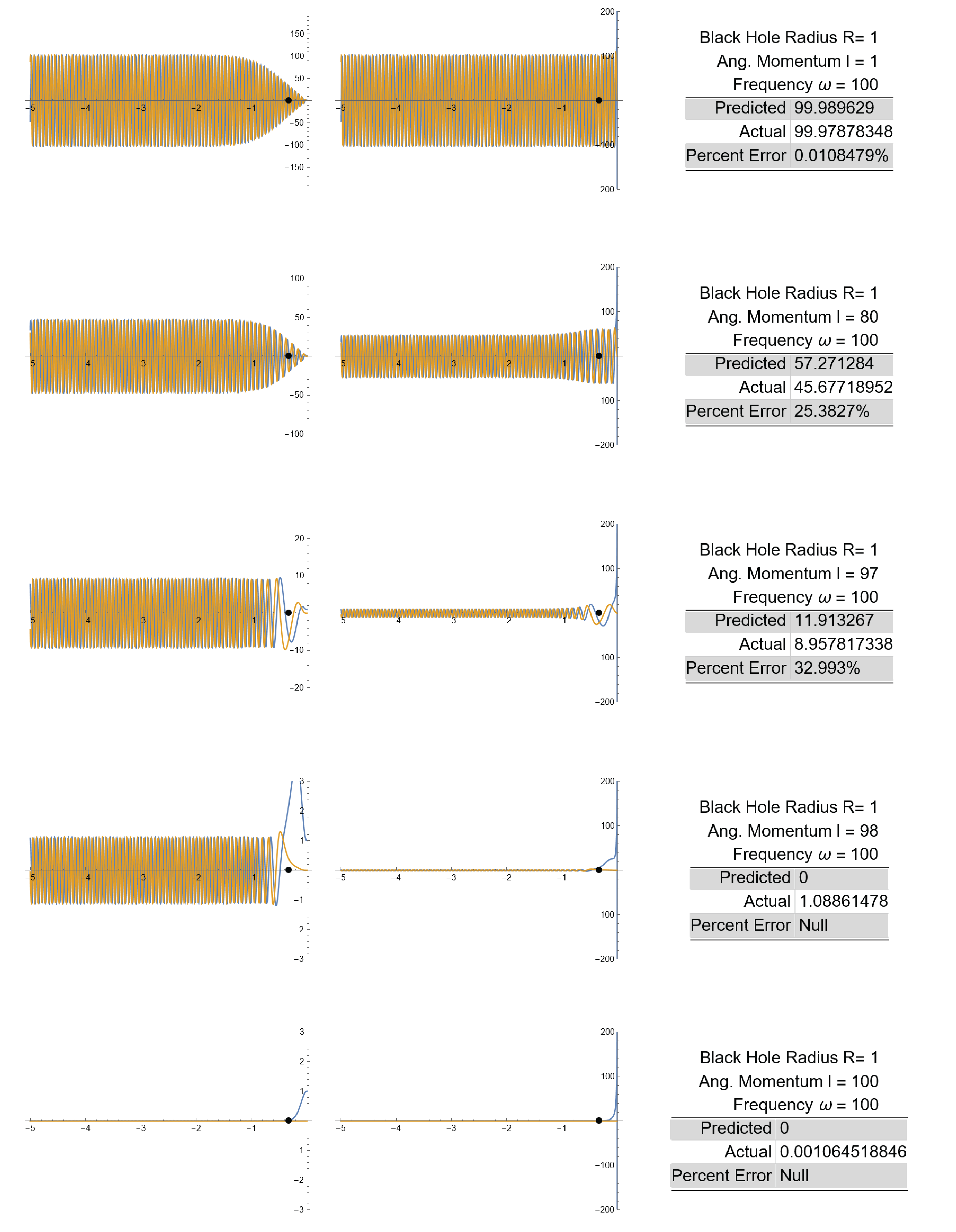
Figure 4: Here we present representative solutions to the differential equations for $\psi(r_{*})$ and $\phi(r_{*})$, which satisfy the Schrödinger-type equation (38), on the right, and the Helmholtz-type equation, (36), on the left. The black dot is the photon sphere location. For the vast majority of cases the plot was like the top figure, where $\psi(r_{*})$ was constant and division by the tortoise coordinate produced $\phi(r_{*})$. The inaccuracy in the approximation arises due to a “bulge” at the photon sphere, visible in the second plot from the top, which begins to form before the phase transition at the onset point. Note the solutions to the wave equation, $\phi$, are trapped outside the photon sphere (the black dot) beyond the onset point.

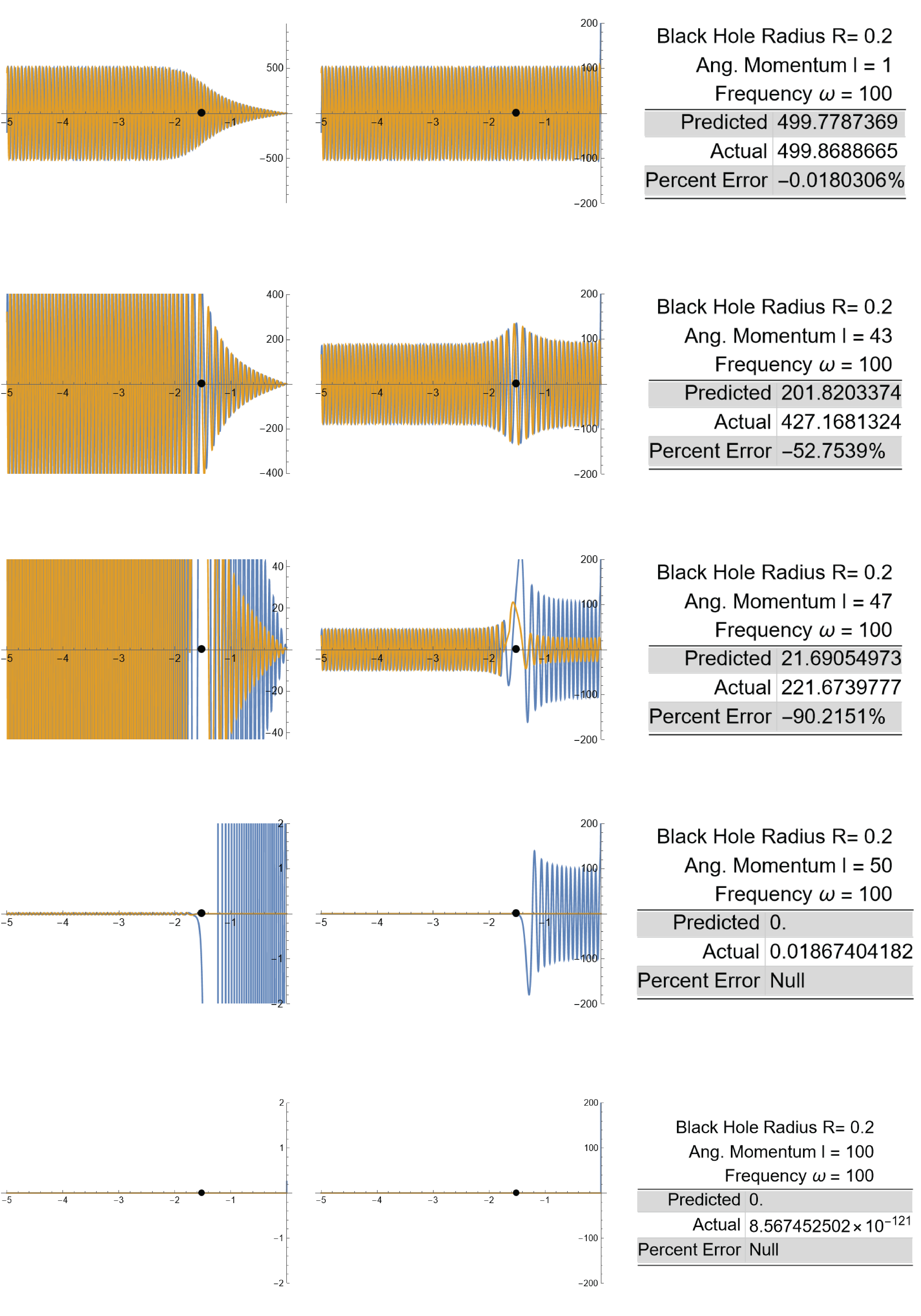
Figure 5: Here we present representative solutions to the differential equations for $\psi(r_{*})$ and $\phi(r_{*})$, which satisfy the Schrödinger-type equation (38), on the right, and the Helmholtz-type equation (36), on the left. The black dot is the photon sphere location. For the vast majority of cases the plot was like the top figure, where $\phi(r_{*})$ was constant and division by the tortoise coordinate produced $\phi=\phi(r_{*})$. The inaccuracy in the approximation arises due to a “bulge” at the photon sphere which appears earlier for smaller black holes. Note the decay of the complex part of the amplitude, and that transitions for small black holes at $b=1$ and $b=1+1/27M^{2}$ are more distinct and extreme.

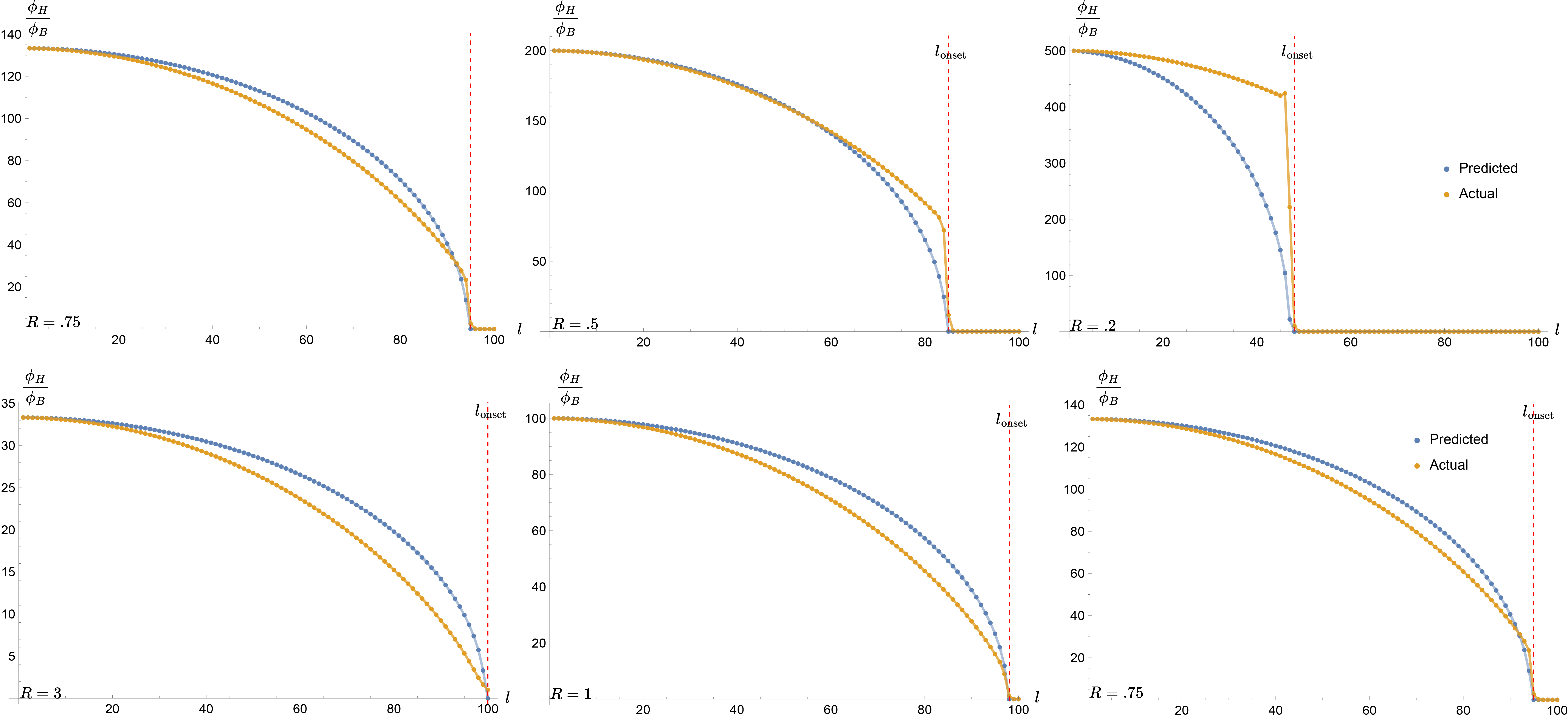
Figure 6: We present the ratios of the amplitudes of the field values $\phi(r_{*})_{H}$ at the horizon to the amplitudes of their sources at the AdS boundary $\phi(r_{*})_{B}$. It is clear that the amplification formula is highly predictive – it correctly predicts the endpoints and the (mostly) monotonic behavior. The bottom three plots show the amplitudes for two black holes near the Hawking–Page transition (at $R=1$) and one significantly above it at $R=3$. The top row shows three black holes below the Hawking–Page transition – note that the approximation begins to break down for $M=0.2$. This is because small AdS black holes have a large spike in their effective potential near the photon sphere – see Figure 3. Some exceptions exist to monotonic behavior at the transition point, where fields near the photon sphere can fluctuate wildly before decaying to zero.

References

- (1) J. M. Bardeen, W. H. Press and S. A. Teukolsky, Rotating black holes: Locally nonrotating frames, energy extraction, and scalar synchrotron radiation, Astrophys. J. 178 (1972) 347.
- (2) C. W. Misner, K. S. Thorne and J. A. Wheeler, Gravitation. W. H. Freeman, San Francisco, 1973.
- (3) J. B. Hartle, Gravity: an introduction to Einstein’s general relativity, 2003.
- (4) K. Hashimoto, S. Kinoshita and K. Murata, Imaging black holes through the AdS/CFT correspondence, Phys. Rev. D 101 (2020) 066018 [1811.12617].
- (5) K. Hashimoto, S. Kinoshita and K. Murata, Einstein Rings in Holography, Phys. Rev. Lett. 123 (2019) 031602 [1906.09113].
- (6) V. Perlick, Gravitational lensing from a spacetime perspective, Living Rev. Rel. 7 (2004) 9.
- (7) A. Grenzebach, V. Perlick and C. Lämmerzahl, Photon Regions and Shadows of Kerr-Newman-NUT Black Holes with a Cosmological Constant, Phys. Rev. D 89 (2014) 124004 [1403.5234].
- (8) A. Grenzebach, V. Perlick and C. Lämmerzahl, Photon Regions and Shadows of Accelerated Black Holes, Int. J. Mod. Phys. D 24 (2015) 1542024 [1503.03036].
- (9) M. D. Johnson et al., Universal interferometric signatures of a black hole’s photon ring, Sci. Adv. 6 (2020) eaaz1310 [1907.04329].
- (10) S. E. Gralla and A. Lupsasca, Lensing by Kerr Black Holes, Phys. Rev. D 101 (2020) 044031 [1910.12873].
- (11) E. Himwich, M. D. Johnson, A. Lupsasca and A. Strominger, Universal polarimetric signatures of the black hole photon ring, Phys. Rev. D 101 (2020) 084020 [2001.08750].
- (12) S. Hadar, D. Kapec, A. Lupsasca and A. Strominger, Holography of the photon ring, Class. Quant. Grav. 39 (2022) 215001 [2205.05064].
- (13) D. Kapec, A. Lupsasca and A. Strominger, Photon rings around warped black holes, Class. Quant. Grav. 40 (2023) 095006 [2211.01674].
- (14) Event Horizon Telescope collaboration, First M87 Event Horizon Telescope Results. I. The Shadow of the Supermassive Black Hole, Astrophys. J. Lett. 875 (2019) L1 [1906.11238].
- (15) Event Horizon Telescope collaboration, First Sagittarius A* Event Horizon Telescope Results. I. The Shadow of the Supermassive Black Hole in the Center of the Milky Way, Astrophys. J. Lett. 930 (2022) L12.
- (16) V. Perlick and O. Y. Tsupko, Calculating black hole shadows: Review of analytical studies, Physics Reports 947 (2022) 1.
- (17) E. Berti, V. Cardoso and A. O. Starinets, Quasinormal modes of black holes and black branes, Class. Quant. Grav. 26 (2009) 163001 [0905.2975].
- (18) B. F. Schutz and C. M. Will, Black Hole Normal Modes: A Semianalytic Approach, Astrophys. J. Lett. 291 (1985) L33.
- (19) S. Iyer and C. M. Will, Black Hole Normal Modes: A WKB Approach. 1. Foundations and Application of a Higher Order WKB Analysis of Potential Barrier Scattering, Phys. Rev. D 35 (1987) 3621.
- (20) S. Iyer, Black Hole Normal Modes: A WKB Approach. 2. Schwarzschild Black Holes, Phys. Rev. D 35 (1987) 3632.
- (21) E. W. Leaver, An Analytic representation for the quasi normal modes of Kerr black holes, Proc. Roy. Soc. Lond. A 402 (1985) 285.
- (22) E. W. Leaver, Solutions to a generalized spheroidal wave equation: Teukolsky’s equations in general relativity, and the two-center problem in molecular quantum mechanics, Journal of mathematical physics 27 (1986) 1238.
- (23) E. W. Leaver, Spectral decomposition of the perturbation response of the Schwarzschild geometry, Phys. Rev. D 34 (1986) 384.
- (24) R. G. Daghigh, M. D. Green and J. C. Morey, Calculating quasinormal modes of Schwarzschild anti–de Sitter black holes using the continued fraction method, Phys. Rev. D 107 (2023) 024023 [2209.09324].
- (25) Y. Decanini and A. Folacci, Quasinormal modes of the BTZ black hole are generated by surface waves supported by its boundary at infinity, Phys. Rev. D 79 (2009) 044021 [0901.1642].
- (26) R. H. Price, Nonspherical Perturbations of Relativistic Gravitational Collapse. II. Integer-Spin, Zero-Rest-Mass Fields, Phys. Rev. D 5 (1972) 2439.
- (27) E. S. C. Ching, P. T. Leung, W. M. Suen and K. Young, Late time tail of wave propagation on curved space-time, Phys. Rev. Lett. 74 (1995) 2414 [gr-qc/9410044].
- (28) E. S. C. Ching, P. T. Leung, W. M. Suen and K. Young, Wave propagation in gravitational systems: Late time behavior, Phys. Rev. D 52 (1995) 2118 [gr-qc/9507035].
- (29) G. T. Horowitz and V. E. Hubeny, Quasinormal modes of AdS black holes and the approach to thermal equilibrium, Phys. Rev. D 62 (2000) 024027 [hep-th/9909056].
- (30) S. A. Hartnoll, A. Lucas and S. Sachdev, Holographic quantum matter. MIT press, 2018.
- (31) F. Denef, S. A. Hartnoll and S. Sachdev, Black hole determinants and quasinormal modes, Class. Quant. Grav. 27 (2010) 125001 [0908.2657].
- (32) C. Keeler and G. S. Ng, Partition Functions in Even Dimensional AdS via Quasinormal Mode Methods, JHEP 06 (2014) 099 [1401.7016].
- (33) C. Keeler, P. Lisbao and G. S. Ng, Partition functions with spin in AdS2 via quasinormal mode methods, JHEP 10 (2016) 060 [1601.04720].
- (34) P. Kovtun and L. G. Yaffe, Hydrodynamic fluctuations, long time tails, and supersymmetry, Phys. Rev. D 68 (2003) 025007 [hep-th/0303010].
- (35) D. Mukherjee and K. Narayan, Hyperscaling violation, quasinormal modes and shear diffusion, JHEP 12 (2017) 023 [1707.07490].
- (36) T. Andrade and A. Krikun, Coherent vs incoherent transport in holographic strange insulators, JHEP 05 (2019) 119 [1812.08132].
- (37) G. Policastro, D. T. Son and A. O. Starinets, From AdS/CFT correspondence to hydrodynamics. 2. Sound waves, JHEP 12 (2002) 054 [hep-th/0210220].
- (38) C. P. Herzog, The Sound of M theory, Phys. Rev. D 68 (2003) 024013 [hep-th/0302086].
- (39) P. K. Kovtun and A. O. Starinets, Quasinormal modes and holography, Phys. Rev. D 72 (2005) 086009 [hep-th/0506184].
- (40) M. Kaminski, K. Landsteiner, J. Mas, J. P. Shock and J. Tarrio, Holographic Operator Mixing and Quasinormal Modes on the Brane, JHEP 02 (2010) 021 [0911.3610].
- (41) I. Amado, M. Kaminski and K. Landsteiner, Hydrodynamics of Holographic Superconductors, JHEP 05 (2009) 021 [0903.2209].
- (42) M. J. Bhaseen, J. P. Gauntlett, B. D. Simons, J. Sonner and T. Wiseman, Holographic Superfluids and the Dynamics of Symmetry Breaking, Phys. Rev. Lett. 110 (2013) 015301 [1207.4194].
- (43) V. Cardoso, A. S. Miranda, E. Berti, H. Witek and V. T. Zanchin, Geodesic stability, Lyapunov exponents and quasinormal modes, Phys. Rev. D 79 (2009) 064016 [0812.1806].
- (44) J. M. Bardeen, Interpreting the semi-classical stress-energy tensor in a Schwarzschild background, implications for the information paradox, 1808.08638.
- (45) H. Falcke, F. Melia and E. Agol, Viewing the shadow of the black hole at the galactic center, Astrophys. J. Lett. 528 (2000) L13 [astro-ph/9912263].
- (46) H. Geng, A. Karch, C. Perez-Pardavila, S. Raju, L. Randall, M. Riojas and S. Shashi, Information Transfer with a Gravitating Bath, SciPost Phys. 10 (2021) 103 [2012.04671].
- (47) H. Geng, A. Karch, C. Perez-Pardavila, S. Raju, L. Randall, M. Riojas and S. Shashi, Inconsistency of islands in theories with long-range gravity, JHEP 01 (2022) 182 [2107.03390].
- (48) A. Karch, C. Perez-Pardavila, M. Riojas and M. Youssef, Subregion entropy for the doubly-holographic global black string, JHEP 05 (2023) 195 [2303.09571].
- (49) I. R. Klebanov and E. Witten, AdS/CFT correspondence and symmetry breaking, Nucl. Phys. B 556 (1999) 89 [hep-th/9905104].
- (50) V. Ferrari and B. Mashhoon, New approach to the quasinormal modes of a black hole, Phys. Rev. D 30 (1984) 295.
- (51) N. Cruz, M. Olivares and J. R. Villanueva, The golden ratio in Schwarzschild–Kottler black holes, Eur. Phys. J. C 77 (2017) 123 [1701.03166].
- (52) C. Keeler, V. L. Martin and A. Svesko, Connecting quasinormal modes and heat kernels in 1-loop determinants, SciPost Phys. 8 (2020) 017 [1811.08433].
- (53) C. Keeler, V. L. Martin and A. Svesko, BTZ one-loop determinants via the Selberg zeta function for general spin, JHEP 10 (2020) 138 [1910.07607].
- (54) V. L. Martin and A. Svesko, Higher spin partition functions via the quasinormal mode method in de Sitter quantum gravity, SciPost Phys. 9 (2020) 039 [2004.00128].
- (55) M. S. Churilova, Quasinormal modes of the test fields in the consistent 4D Einstein–Gauss-Bonnet–(anti)de Sitter gravity, Annals Phys. 427 (2021) 168425 [2004.14172].
- (56) K. Hashimoto, K. Sugiura, K. Sugiyama and T. Yoda, Photon sphere and quasinormal modes in AdS/CFT, 2307.00237.
- (57) D. J. Griffiths and D. F. Schroeter, Introduction to quantum mechanics. Cambridge university press, 2018.
- (58) K. D. Kokkotas and B. G. Schmidt, Quasinormal modes of stars and black holes, Living Rev. Rel. 2 (1999) 2 [gr-qc/9909058].