Accretion Properties and Estimation of Spin of Galactic Black Hole Candidate Swift J1728.9–3613 with NuSTAR during its 2019 outburst

Abstract

Black hole X-ray binaries (BHXRBs) play a crucial role in understanding the accretion of matter onto a black hole. Here, we focus on exploring the transient BHXRB Swift J1728.9–3613 discovered by Swift/BAT and MAXI/GSC during its January 2019 outburst. We present measurements on its accretion properties, long time-scale variability, and spin. To probe these properties we make use of several NICER observations and an unexplored data set from NuSTAR, as well as long term light curves from MAXI/GSC. In our timing analysis we provide estimates of the cross-correlation functions between light curves in various energy bands. In our spectral analysis we employ numerous phenomenological models to constrain the parameters of the system, including flavours of the relativistic reflection model Relxill to model the Fe K$\alpha$ line and the $>15$ keV reflection hump. Our analysis reveals that: (i) Over the course of the outburst the total energy released was $\sim 5.2\times 10^{44}$ ergs, corresponding to roughly 90% the mass of Mars being devoured. (ii) We find a continuum lag of $8.4\pm 1.9$ days between light curves in the $2-4$ keV and $10-20$ keV bands which could be related to the viscous inflow time-scale of matter in the standard disc. (iii) Spectral analysis reveals a spin parameter of $\sim 0.6-0.7$ with an inclination angle of $\sim 45^{\circ}-70^{\circ}$, and an accretion rate during the NuSTAR observation of $\sim 17\%~{}L_{\rm Edd}$.

1 Introduction

Black hole X-ray binaries (BHXRBs) are a class of astrophysical objects in which a black hole and a main sequence star are gravitationally bound. These systems make ideal laboratories for studying the physics of accretion and matter in the presence of an extreme gravitational well, in addition to testing the predictions of general relativity. BHXRBs are further categorized into transient and persistent classes. The transient class remains dormant for most of its lifetime, except for occasional outbursts where the luminosities ($L_{\rm X}$) reach beyond $10^{35}$ erg s^-1(e.g., Tetarenko et al., 2016). These outbursts and their spectral evolution are traced through the so-called ‘q’ or hardness–intensity diagram (e.g., Homan et al., 2001; Remillard & McClintock, 2006). A full outburst starts with a low/hard state followed by an intermediate state reaching to the high/soft state while rising to the peak luminosity. During the declining phase, the path reverses ending with the hard state. ‘Failed’ or hard/low state only outbursts are those where high/soft state remains absent (see Alabarta et al., 2021, and references therein). Energy dependent variations in count rates are a universal feature of outbursting BHXRBs, which are usually attributed to their accretion properties. A few major physical drivers of accretion are viscosity (e.g., Shakura & Sunyaev, 1973; Smith et al., 2002; Chatterjee et al., 2020), electron cloud temperature and optical depth (Sunyaev & Titarchuk, 1980, 1985), the Compton cooling rate of the cloud (e.g., Chakrabarti & Titarchuk, 1995; Garain et al., 2012, 2014). In general, measurements of such parameters are performed using long term light-curve variations and detailed spectral studies using various phenomenological or physical models.

Apart from accretion properties, outbursting BHXRBs also provide a chance to measure the intrinsic properties of the black hole itself, e.g. mass ($M_{\rm BH}$) and spin ($a^{*}$). The dynamical method, wherein mass is obtained using radial velocity measured from absorption lines in the spectrum from the companion star, provides the most accurate measure of the mass (Casares & Jonker, 2014). One can also use dips and eclipses in the light curve to predict the mass ratio and inclination of the binary system (Horne, 1985). However, only around 20 BHXRBs are measured this way (e.g., Corral-Santana et al., 2016). Apart from the dynamical method, one can measure the mass using spectral fitting (e.g., Kreidberg et al., 2012; Torres et al., 2019; Kubota et al., 1998; Shaposhnikov & Titarchuk, 2007; Jana et al., 2022) or the X-ray reverberation method (Mastroserio et al., 2019). Direct measurement of the spin could be carried out by imaging the shape of the photon sphere or radius of the innermost stable circular orbit (ISCO) (Chan et al., 2013). Using radio interferometry, the EHT-collaboration directly captured images of the supermassive black holes M 87* and our own Sgr A* (see Event Horizon Telescope Collaboration et al. (2019, 2022) and references therein). For galactic BHXRBs, spin is usually measured by X-ray spectroscopy (e.g Draghis et al. (2022)), though in principle X-ray interferometry could be used to produce EHT-style observations that directly image the shape of the BH shadow in some Seyfert galaxies (Uttley et al.,, 2020; den Hartog et al., 2020).

Within X-ray spectroscopy there are two primary methods that have proved successful in measuring black hole spin, namely continuum fitting (e.g., Zhang et al., 1997; McClintock et al., 2006; Steiner et al., 2014) and relativistic reflection (e.g., Fabian et al., 1989; Miller et al., 2012; Reynolds, 2021). In continuum fitting, the inner edge of the accretion disc or ISCO ($r_{\rm in}$) is measured through the inner disc temperature. The optically thick and geometrically thin accretion disc considers the relativistic form prescribed by (Novikov & Thorne, 1973) where the spin influences $r_{\rm in}$. For extreme prograde motion (i.e. $a\rightarrow 1$), $r_{\rm in}$, marginally stable and bound orbits and, the photon sphere merge into the surface of the event horizon. As the inner radius becomes smaller, the excess binding energy loss, spent into heating the accretion disc, becomes increasingly larger while approaching $r_{\rm in}$. The corresponding temperature $T_{\rm in}$ can then be measured using relativistic models like Kerrbb (Zhang et al., 1997; Li et al., 2005). This method was employed to measure the spins of LMC X–1 (Gou et al., 2009; Mudambi et al., 2020), H 1743-322 (Steiner et al., 2009), GRS 1915+105 (Sreehari et al., 2020), LMC X–1 (Jana et al., 2021a), LMC X–3 (Bhuvana et al., 2021), and MAXI J1820+070 (Zhao et al., 2021).

In contrast to continuum fitting, the relativistic reflection method instead models the spectral shape using the blurred iron K$\alpha$ line at 6.4 keV and associated reflection hump above 15 keV (Fabian et al., 1989; George & Fabian, 1991). This fluorescent line distorts due to the gravitational redshift experienced by the reflected spectra of a spinning black hole, with maximal distortion occurring for a maximally spinning prograde orbit. The ‘reflection hump’ arises due to the hard X-ray reflection from the accretion disc. Often the irradiation of the disc shows a profile steeper than $r^{-5}$, invoking a compact corona along the rotation axis of the black hole. This is the so-called ‘lamp-post’ model of the coronal geometry (Miniutti & Fabian, 2004), and the height and compactness of this corona change alongside other spectral properties (Fabian et al., 2015). As the Doppler effect significantly modifies the observed spectrum with changing inclination (Luminet, 1979; Viergutz, 1993), these models calculate the parameters of the system and modify the iron line profile accordingly. A central assumption invoked in this method is that the inner radius of the accretion disk extends all the way to the inner most stable circular orbit or ISCO. This need not be the case, especially in the low/hard state (e.g. Zdziarski & Marco, 2020; Done et al., 2007). The spectroscopic reflection model Relxill (García et al., 2013; Dauser et al., 2014; García et al., 2014) provides a measure of the iron abundance ($A_{\rm Fe}$) within the disc, and various flavours of disc/emissivity profiles can be assumed. Within the past few years, Relxill has successfully measured the spin of many galactic black holes, such as MAXI J1535–571 (Miller et al., 2018), Cygnus X–1 (Tomsick et al., 2018), XTE J1752–223 (García et al., 2018), GX 339–4 (García et al., 2019), MAXI J1631–479 (Xu et al., 2020), XTE J1908–094 (Draghis et al., 2021), MAXI J1813–095 (Jana et al., 2021b). Most recently, Draghis et al. (2022) reported spins of ten new Galactic black hole candidate using the Relxill model. Apart from these two, one can measure spin using timing properties where low-frequency Quasi Periodic Oscillations (QPOs) are assumed to originate from  Lense-Thirring precession (Ingram et al., 2009).

Swift J1728.9–3613  or MAXI J1728–36 went into outburst on 17 January 2019 and continued until June 2019. The source was reported by Swift/BAT on 28 January 2019 (Barthelmy et al., 2019). However, it was initially discovered by MAXI/GSC on 26 January 2019 (Negoro et al., 2019). On 31 January 2019, MeerKAT detected the radio counterpart of the source with a magnitude of $11.2\pm 0.6$ mJy at 1.28 GHz (Bright et al., 2019). Integral observed the source on 19 February 2019 and detected the source flux as $103\pm 4$ mCrab in the $20-40$ keV range (Ducci et al., 2019). Following the MAXI and Swift detection, NICER has been monitoring the source since 29 January 2019 (Enoto et al., 2019), producing a total of 103 observations. Out of these, $\sim 70$ of them lie within the outbursting period. An optical counterpart with a magnitude of 16.7 was observed on 28 January 2019 by the 60 cm BOOTES-3/YA robotic telescope (Hu et al., 2019). Recently, Saha et al. (2022) analyzed NICER spectra of Swift J1728.9–3613  during the outburst and obtained a lower mass limit for the compact object of $4.6~{}M_{\odot}$, obtained assuming $a^{*}=0$ from the inner radius of the disk and a distance of $\sim 10$ kpc. This estimate further strengthens Swift J1728.9–3613’s candidacy as a BHXRB. NuSTAR observed Swift J1728.9–3613  on 3 February 2019 but has thus far remained unexplored. This is the observation we utilized to estimate the spin and accretion properties.

In this paper, we concentrate on the MAXI/GSC light curve to explore the long time scale variability. We explored the first two observations of NICER to understand the beginning of the outburst. Later, we systematically examine the NuSTAR data to extract accretion disc properties and spin using numerous models such as Diskbb, Cutoffpl, Nthcomp, and Relxill. The paper is structured as follows. The data analysis process is briefly described in Section 2. Results obtained from MAXI/GSC light curve are presented in Section 3.1. Spectral analysis with NICER is presented in Section 3.2. Spectral properties are analyzed and constrained in Section 3.3, while Relxill is employed in Section 3.3.3. Finally, we draw our conclusions and discuss our results in Section 4. All errors associated with model parameters are quoted at the 90% confidence level unless otherwise stated.

Table 1: Log of Observations of Swift J1728.9–3613

Instrument	Date (UT)	Obs ID	Exposure (ks)	Count s-1
NICER/XTI	2019-01-29	1200550101	1.86	$581.7\pm 0.7$
NICER/XTI	2019-01-30	1200550102	13.7	$992.0\pm 0.4$
NuSTAR	2019-02-03	90501303002	55.9	$144.7\pm 0.02$

2 Observations and Data Reduction

NuSTAR observed Swift J1728.9–3613 on 3 February 2019 for a total exposure of 55.9 ks (see Table 1). NuSTAR is a hard X-ray focusing telescope, consisting of two identical modules: FPMA and FPMB (Harrison et al., 2013). The raw data were reprocessed with the NuSTAR Data Analysis Software (NuSTARDAS, version 1.4.1). Cleaned event files were generated and calibrated by using the standard filtering criteria in the nupipeline task and the latest calibration data files available in the NuSTAR calibration database (CALDB). The source and background products were extracted by considering circular regions with radii 60 arcsec and 90 arcsec, at the source coordinates and away from the source, respectively. The spectra and light curves were extracted using the nuproduct task. We re-binned the spectra with 25 counts per bin by using the grppha task. Additionally, we divided the light-curves in two segments using xselect and run nuproduct using user defined gti files.

Following the discovery of Swift J1728.9–3613, NICER began to monitor the source. We analysed the first two of the 70 NICER observations. NICER is a soft X-ray telescope whose primary X-ray Timing Instrument (XTI) consists of 56 identical FPMs (50 of which are functional) that record the energies of arriving photons, as well as their time of arrival to within 300 ns of UTC (Gendreau et al., 2012). Raw data were processed with the NICER Data Analysis Software (NICERDAS, version 9). Cleaned event files were generated with standard filtering criteria in the nicerl2 task, while background files were generated with the nibackgen3C50 task. Response files were generated with the nicerarf and nicerrmf tasks. Spectra and light curves were extracted with xselect and spectra were rebinned with 25 counts per bin using the grppha task. We have not applied any systematic on NuSTAR or NICER data.

3 Results and Discussion

3.1 Long Term Delay

MAXI/GSC (Matsuoka et al., 2009) has monitored the source daily and provided one day binned light curves at various energy ranges. From these curves, as presented in the top panel of Fig. 1, we observed that the peak of the outburst occurred within 10-12 days of the beginning. Comparable to other canonical outbursts, rate variations were observed in various energy ranges. During the peak luminosity in the high/soft state, the hard 10-20 keV counts were substantially less than the softer 2-4 keV counts. In total, we found the outburst lasted for about 150 days starting from MJD 58500 to 58150.

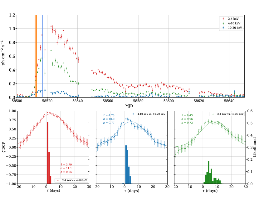
Figure 1: Top panel: MAXI/GSC light curves of Swift J1728.9–3613 during the outburst in three different energy bands, binned at 1 day. The blue vertical line represents the date of the primary NuSTAR observation analyzed in Section 3.3, while the orange lines show when the two NICER observations analyzed in Section 3.2 were taken. Bottom panels: Estimations of the cross–correlation functions between light curves of the indicated energy bands and likelihood distributions of the true time lags. Estimation was performed with the $\zeta$-transformed discrete correlation function ($\zeta$-DCF) and its associated likelihood (PLIKE) algorithm from Alexander (2014). $\tilde{\tau}$ and $\sigma$ are the mean and standard deviation of the Gaussian fits, while $\rho$ is the maximum DCF value.

The MAXI/GSC light curves can be used to obtain an estimate for the amount of energy released by the outburst in each energy band as

$$E_{i}=4\pi D^{2}\tilde{E}_{i}\int_{{\rm MJD}_{\rm start}}^{{\rm MJD}_{\rm stop}}L_{i}(t)dt$$

where $D$ is the distance to the source, $\tilde{E}_{i}$ is the average photon energy in the $i^{\rm th}$ band, and $L_{i}$ is the corresponding MAXI/GSC light curve. Assuming a distance of 10 kpc and an average photon energy of 3.0 keV, 7.0 keV, and 15 keV in each energy band respectively, we calculate an energy output of $\sim 2.1\times 10^{44}$ ergs in the $2-4$ keV band, $\sim 2.2\times 10^{44}$ ergs in the $4-10$ keV band, and $\sim 9.0\times 10^{43}$ ergs in the $10-20$ keV band, all over the course of the entire outburst. Considering all energy bands, the total energy released is $\sim 5.2\times 10^{44}$ ergs, which translates to $5.8\times 10^{26}$ g of mass assuming a mass-to-radiation conversion efficiency of 0.1 (Reynolds, 2021). The converted matter is equivalent to $2.9\times 10^{-7}M_{\odot}$ or 91% of the mass of Mars. However, the bolometric luminosity should be higher than what we have calculated from X-rays. Thus, it is expected that our estimation of the matter conversion is moderately reserved.

We inspected the time delays among the energy bands using the $\zeta$-DCF algorithm (Alexander, 2014), presented in the bottom panels of Fig. 1. A positive delay refers to the softer component arriving later, while the reverse indicates delayed arrival of the harder component. The $2-4$ keV light curve correlates with both $4-10$ and $10-20$ keV light curves, having maximum correlation coefficients ($\rho$) of $0.95$ and $0.72$ respectively. The peak delays ($\tilde{\tau}$) between the corresponding light curves were found to be $(3.7\pm 0.8)$ and $(8.4\pm 1.9)$ days, with standard deviations $11.1$ and $9.9$ days respectively. A similar correlated pattern was also observed between $4-10$ and $10-20$ keV light curves with maximum coefficient, delay, and width $\rho=0.77$, $\tilde{\tau}=(4.7\pm 1.1)$ days, $\sigma=10.0$ days respectively. This delay is consistent with what we would expect examining the other two light curves, i.e. $8.4\;{\rm days}-3.7\;{\rm days}=4.7\;{\rm days}$. We should note that $\sigma$ here refers to the estimated width of the cross-correlation function itself, whereas the errors associated with the true delays are estimated from the width of the corresponding likelihood distribution. These distributions were calculated with the PLIKE algorithm, also presented by Alexander (2014). Our analysis showed that harder ($10-20$ keV) radiation as a whole arrived before its softer counterpart. The magnitude of the delay increased with increasing differences in X-ray energy, exhibiting a maximum delay between the $2-4$ and $10-20$ keV photons. An accreting BHXRB spectrum is typically approximated by the sum of a hard power-law and soft blackbody disk component, and from the light curve analysis we can infer that the harder spectral component dominated the rising phase before giving way to more prominent soft disk emission. This scenario is similar to what was observed earlier in the outburst profiles of GX 339–4, XTE J1650–500 (Smith et al., 2002; Chatterjee et al., 2020). A possible reason for this delayed peak in soft emission could be the viscous delay with which the standard disc spirals inward before heating enough to glow in the X-ray. Influenced by the viscous delay, the disc gradually modifies the spectral and temporal properties, triggering the outburst profile of the BHXRB (Smith et al., 2002). The left panel of Fig. 2 shows the variation in hardness ratio (HR) vs. intensity (in terms of the accretion rate $\dot{M}=L/L_{\rm Edd}$) over the full outburst as observed by MAXI/GSC, and illustrates a typical ‘q’ diagram for an outbursting BHXRB.

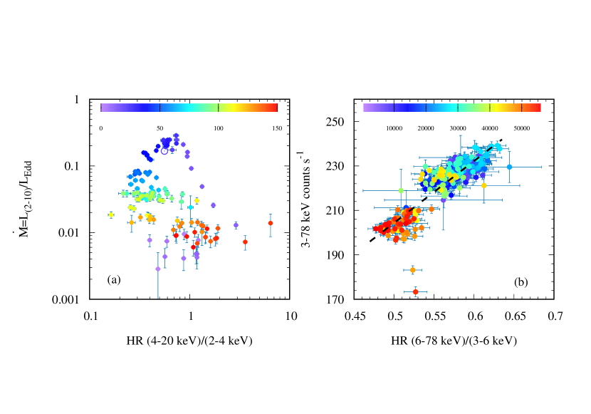
Figure 2: Left Panel (a): Hardness–accretion rate diagram of Swift J1728.9–3613 over the course of its outburst, produced with MAXI/GSC observations. The MAXI hardness ratio (HR) is defined as the ratio of count rates in the $4-20$ keV and $2-4$ keV bands. Colour represents progression of the outburst through time (MJD-58500 days) as indicated at the top. The maximum disc accretion rate was $\dot{M}_{\rm max}=0.28~{}L_{\rm Edd}$ during peak luminosity. The primary NuSTAR observation is marked with $\odot$. Right Panel (b): Hardness–intensity diagram (HID) for the first NuSTAR observation of the Swift J1728.9–3613 outburst. Points are binned at 100s with the NuSTAR HR defined as the ratio of count rates in the $6-78$ keV and $3-6$ keV bands. Colour represents progression through time as indicated at the top, in seconds. The dashed line through the data is the best fit having a slope and intercept of $278.2\pm 10.5$ and $65.2\pm 6.0$ counts/s, respectively.

3.2 NICER

As mentioned previously, the X-ray spectrum of a BHXRB is typically approximated with the sum of a multi-colour disc blackbody (MCD) and power-law component. Reprocessed or reflected emission may also be observed, such as a Fe K$\alpha$ line at $\sim 6.4$ keV, a reflection hump at $\sim 15-40$ keV (see bottom panel of Fig. 4), and in our case, an apparent Ni emission line at $\sim 8$ keV (Corliss & Sugar, 1981; Molendi et al., 2003; Medvedev et al., 2018). Spectral analysis was carried out in HEASEARC’s spectral analysis package XSPEC version 12.12.1 (Arnaud, 1996). We used the Tbabs model to account for interstellar absorption with the WILM abundance (Wilms et al., 2000) and the cross-section of Verner et al. (1996). The MCD component was handled with the Diskbb model, and is included in all spectral models presented in this paper.

The first two NICER observations of Swift J1728.9–3613 were taken on MJD 58512 and MJD 58513 respectively, which correspond to the beginning of the rising phase of the outburst – or the low/hard state. We fit the data for the first two observations in the $0.3-10.0$ keV range with an absorbed MCD and power law model [Tbabs*(Diskbb + Powerlaw)]. This returned an inner disc temperature of $T_{\rm in}=1.05_{-0.02}^{+0.03}$ keV for the first observation and $T_{\rm in}=1.229_{-0.006}^{+0.006}$ keV for the second. We find a reduction in photon index from $\Gamma=2.02_{-0.07}^{+0.06}$ to $1.72_{-0.08}^{+0.08}$, with normalization varying from $\sim 1.7$ to $\sim 0.9~{}{\rm ph~{}keV^{-1}~{}cm^{-2}}$; hydrogen column density stayed approximately constant ($n_{\rm H}=4.67_{-0.07}^{+0.07}\times 10^{-22}{\rm cm^{-2}}$ to $4.58_{-0.04}^{+0.04}\times 10^{-22}{\rm cm^{-2}}$). Table 2 contains detailed results for each fit, along with their $\chi^{2}$ value per degree of freedom (dof) and model flux. Removing the MCD component from the model substantially worsens both fits, giving an F–statistic of $\sim 200$ and $\sim 3000$ for the first two observations respectively. This indicates the presence of a rapidly growing standard accretion disc at the beginning of the outburst.

Table 2: NICER Spectral Analysis Results: Diskbb+Powerlaw

Observation ID	$n_{\rm H}$ ($10^{-22}{\rm cm^{-2}}$)	$T_{\rm in}$ (keV)	normdiskbb	$\Gamma$	normPL	$\chi^{2}/$dof	$F_{2-10}$ ($10^{-9}$ ergs cm-2)
1200550101	$4.67_{-0.07}^{+0.07}$	$1.05_{-0.02}^{+0.03}$	$109_{-20}^{+20}$	$2.02_{-0.07}^{+0.06}$	$1.7_{-0.3}^{+0.3}$	891/902	$4.498_{-0.010}^{+0.010}$
1200550102	$4.58_{-0.04}^{+0.04}$	$1.229_{-0.006}^{+0.006}$	$215_{-8}^{+8}$	$1.72_{-0.08}^{+0.08}$	$0.9_{-0.2}^{+0.2}$	1008/944	$6.177_{-0.014}^{+0.014}$

$F_{2-10}$ is the total model flux in the $2-10$ keV range.

3.3 NuSTAR

We performed the spectral analysis of the NuSTAR data in the $3-78$ keV energy range. The right panel of Fig. 2 shows the variation in HR vs. count rate throughout the primary NuSTAR observation, with points binned at 100s. We observe that during the observation HR and intensity were positively correlated, lying along the line with slope, intercept, correlation coefficient, and null hypothesis probability $(278.2\pm 10.5)$, $(65.2\pm 6.0)$ counts/s, $r=0.877$, and $p<10^{-5}$ respectively. Correlation between these two parameters is typical of BHXRBs during intermediate spectral states where disc-corona coupling becomes stronger (Churazov et al., 2001; Taylor et al., 2003). In Section 3.3.1 we resolve the spectrum between the two regions in the HR diagram with unfolded spectra from both regions presented in Fig. 3. Section 3.3.2 is dedicated to examining the full time-averaged spectrum of the observation using several non-relativistic models, and in Section 3.3.3 we explore the same spectrum with several flavours of the Relxill model family. Gaussian components are included to model the Fe and Ni emission lines where necessary in all non-relativistic models. Fig. 4 shows the full spectrum of the NuSTAR observation fit with a simple MCD and power-law model, which disregards all reflected emission. The bottom panel of Fig. 4 displays the residuals of that fit and showcases the reflected emission, i.e. the 6.4 keV Fe K$\alpha$ line and reflection hump above $\sim 15$ keV.

3.3.1 Hardness-Resolved Spectra

The ‘gap’ between data points that occurs at $\sim 45,000$s shows a sudden softening of Swift J1728.9–3613’s spectrum, alongside a reduction in intensity during the observation. We extracted spectra for both regions of the HID (denoting the earlier region i and the later region ii) and fit them with an absorbed MCD and cutoff power law model Cutoffpl, which very roughly approximates the continuum emission of a thermally Comptonized medium. Fig. 3 shows the resulting spectral fits for both regions.

Between regions i and ii the inner disc temperature, photon index, and cutoff energy did not appreciably vary, returning values of $T_{\rm in}=1.195_{-0.011}^{+0.010}$ keV, $\Gamma=2.27_{-0.07}^{+0.07}$, and $E_{\rm cut}=94_{-34}^{+78}$ keV in region i; and $T_{\rm in}=1.216_{-0.005}^{+0.005}$ keV, $\Gamma=2.13_{-0.03}^{+0.03}$, and $E_{\rm cut}=79_{-18}^{+28}$ keV in region ii. In region i we also detected signatures of both the Fe K$\alpha$ line at $E_{\rm Fe}=6.34_{-0.14}^{+0.11}$ keV and the Ni XXVIII line at $E_{\rm Ni}=8.06_{-0.28}^{+0.10}$ keV. In region ii we only detected the Fe K$\alpha$ line (with greater uncertainty) at $E_{\rm Fe}=6.2_{-0.3}^{+0.4}$ keV, and the apparent hydrogen column density changed from $n_{\rm H}=4.19_{-0.12}^{+0.25}\times 10^{-22}{\rm cm^{-2}}$ to a more uncertain $n_{\rm H}=3.14_{-0.7}^{+0.7}\times 10^{-22}{\rm cm^{-2}}$. Between regions we found a reduction in the harder power law component, with normalization varying from $\sim 3.3$ to $\sim 1.5~{}{\rm ph~{}keV^{-1}~{}cm^{-2}}$ (illustrated in Fig. 3). This explains the softening of the spectrum as well as the disappearance of the reprocessed Ni emission line. Variations on this timescale ($\sim 100$s) being primarily influenced by the power-law component are consistent with the findings of Churazov et al. (2001) in the soft state of Cyg X-1. Detailed results of both fits are presented in Table 3.

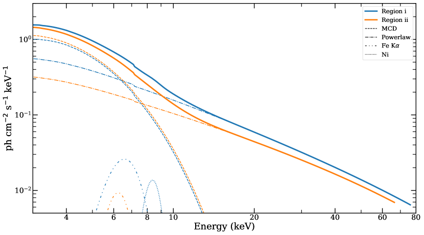
Figure 3: Models (both total and their individual components) for both spectra extracted from region i and region ii of the HID presented in the right panel of Fig. 2.

Table 3: NuSTAR Hardness Resolved Spectral Results

	i	ii
$n_{\rm H}$ ($10^{22}{\rm cm^{-2}}$)	$4.19_{-0.12}^{+0.25}$	$3.8_{-0.7}^{+0.7}$
$T_{\rm in}$ (keV)	$1.195_{-0.011}^{+0.010}$	$1.216_{-0.005}^{+0.005}$
normdiskbb	$313_{-12}^{+13}$	$303_{-6}^{+7}$
$\Gamma$	$2.27_{-0.07}^{+0.07}$	$2.13_{-0.03}^{+0.03}$
$kT_{e}$ (keV)	$94_{-34}^{+78}$	$79_{-18}^{+28}$
normPL (${\rm ph~{}keV^{-1}cm^{-2}}$)	$3.3_{-0.5}^{+0.6}$	$1.54_{-0.07}^{+0.07}$
$E_{\rm Fe}$ (keV)	$6.34_{-0.14}^{+0.11}$	$6.2_{-0.3}^{+0.4}$
$\sigma_{\rm Fe}$ (keV)	$0.80_{-0.07}^{+0.08}$	$0.3_{-0.3}^{+0.5}$
normFe ($10^{-3}$)	$6.5_{-1.4}^{+0.5}$	$1.1_{-0.9}^{+1.0}$
$E_{\rm Ni}$ (keV)	$8.06_{-0.28}^{+0.10}$	-
$\sigma_{\rm Ni}$ (keV)	$0.37_{-0.13}^{+0.19}$	-
normNi ($10^{-3}$)	$1.7_{-0.3}^{+1.2}$	-
$\chi^{2}$/dof	869/887	604/599
$F_{2-10}$ ($10^{-9}$ ergs cm-2)	$9.952_{-0.012}^{+0.012}$	$8.862_{-0.022}^{+0.022}$

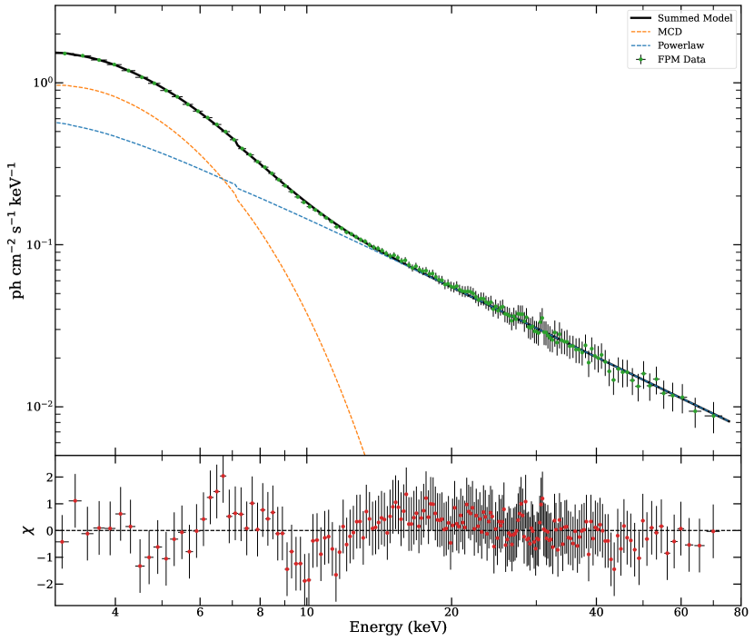
Figure 4: Top panel: Time-averaged unfolded spectrum from FPMB (green) fit with an absorbed MCD and power law model, with no Gaussian components. Both the individual model components as well as their sum are presented. Bottom Panel: Residuals in terms of (data$-$model)/error obtained from spectral analysis for the same model.

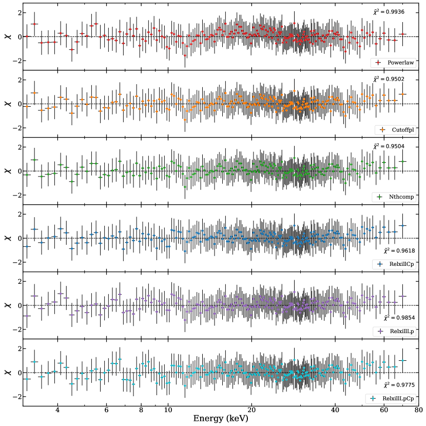
Figure 5: Residuals in terms of (data-model)/error obtained from spectral analysis for the Powerlaw, Cutoffpl, Nthcomp, RelxillCp, RelxillLp, and RelxillLpCp models. Reduced $\chi^{2}$ values ($\tilde{\chi}^{2}$) for each model are quoted in each panel. The first three models (i.e., the non-relativistic ones) include two Gaussian components for the Fe K$\alpha$ and Ni emission lines.

3.3.2 Time averaged spectrum: Phenomenological Models

Examining the entire spectrum of the observation, we first fit the data with an absorbed power–law and MCD model. This model returned a reasonable fit with $\chi^{2}=950$ for 956 degrees of freedom (dof) with estimates of the inner disc temperature $T_{\rm in}=1.185_{-0.010}^{+0.015}$ keV, a photon index of $\Gamma=2.46_{-0.02}^{+0.02}$, and a column density of $n_{\rm H}=4.63_{-0.28}^{+0.28}\times 10^{-22}\mathrm{cm^{-2}}$. We find signatures of the Fe and Ni emission lines at $E_{\rm Fe}=6.48_{-0.02}^{+0.02}$ keV and $E_{\rm Ni}=7.99_{-0.03}^{+0.04}$ keV. The reflection hump was clearly visible in the residuals at energies above $\sim 15$ keV (see Fig. 5). This was repeated with an exponential cutoff power-law component Cutoffpl. This provided no significant improvement to the fit, returning an inner disc temperature of $T_{\rm in}=1.16_{-0.03}^{+0.03}$ keV, a slightly softer photon index of $\Gamma=2.24_{-0.08}^{+0.08}$, cutoff energy $kT_{e}=94_{-39}^{+93}$ keV, and column density $n_{\rm H}=4.32_{-0.23}^{+0.27}\times 10^{-22}\mathrm{cm^{-2}}$; we again find signatures of the Fe and Ni emission lines at $E_{\rm Fe}=6.27_{-0.13}^{+0.16}$ keV and $E_{\rm Ni}=8.0_{-0.2}^{+0.3}$ keV. The reflection hump was still clearly visible in the residuals.

A much better description of continuum emission due to thermal Comptonization is given by the model Nthcomp (Zdziarski et al., 1996), which attempts to simulate the upscattering of photons through the corona from a seed spectrum parameterized by the inner temperature of the accretion disc. The high energy cutoff is parameterized by the electron temperature of the medium. Nthcomp is not a power law, but can still be parameterized with an asymptotic photon index (Życki et al., 1999). Using the inner disc temperature returned by Diskbb, $T_{\rm in}=1.149_{-0.009}^{+0.006}$ keV, as the low energy rollover in Nthcomp, we estimate the hot electron temperature to be $kT_{e}=132_{-123}^{+476}$ keV with photon index $\Gamma=2.36_{-0.01}^{+0.02}$. This model also returned the lowest hydrogen column density of all of the presented models with $n_{\rm H}=3.27_{-0.35}^{+0.91}\times 10^{-22}\mathrm{cm^{-2}}$. For completeness, we may also calculate the optical depth ($\tau$) of the corona as given by Zdziarski et al. (1996),

$$\tau=\sqrt{\frac{9}{4}+\frac{m_{e}c^{2}}{kT_{e}}\frac{3}{(\Gamma-1)(\Gamma+2)}}-\frac{3}{2},$$

returning a value of $\tau=0.55_{-0.42}^{+3.54}$ for the Nthcomp model. The optically thin corona was also proposed for Cyg X-1 (Churazov et al., 2001) during its high/soft state.

We also attempted to fit the spectrum with the non-relativistic reflected power-law model Pexrav from Magdziarz & Zdziarski (1995), alongside a regular power-law component to account for direct coronal emission. Since this model accounts for the reflection and reprocessing of X-rays from the corona by the accretion disc, it can be used to estimate the reflection fraction ($R_{\rm refl}$), defined as the fraction of X-rays reprocessed by the disc vs. those received via direct emission. It also estimates abundances of elements heavier than He, including iron ($A_{\mathrm{Fe}}$), as well as the inclination angle $i$. This model returned a close fit with the reflection hump reduced in the residuals and a $\chi^{2}=916$ for 949 dof. However, most parameters were unable to be constrained. Hence, we opted for relativistic model to estimate those parameters. One of the few parameters that remained well-behaved was the reflection fraction, $R_{\rm refl}=0.48_{-0.06}^{+0.06}$, and we should expect Relxill to estimate reflection fractions of the same order.

Finally, we should note explicitly that in all the aforementioned models, two Gaussian model components were used to model to the Fe K$\alpha$ and Ni emission lines. We observed two more emission lines at 27.9 keV and 30.8 keV having widths of 0.07 keV and 0.06 keV respectively; the normalization of both lines was around $10^{-4}$ ph cm^-2 s^-1. The origin of these emission lines could be attributed to the radioactive isotope ²⁴¹Am, as reported by García et al. (2018); Connors et al. (2022). Similar lines were also observed in AstroSat/LAXPC spectra, which are an instrumental feature (Sreehari et al., 2019). To fit those lines, we added two additional Gaussian components to each model and froze the line energy, width, and normalization as obtained from the Powerlaw model. Detailed results of all spectral fits for this section are presented in the first three columns of Table 4, and the residuals for each model are presented in Fig. 5.

3.3.3 Time averaged spectrum: Relxill

We used different flavors of the relativistic reflection model Relxill (García et al., 2013, 2014; Dauser et al., 2014, 2016) to probe the reprocessed emission more accurately. In this model, the reflection fraction ($R_{\rm refl}$) is given by the ratio between the Comptonized emission to the disc and to the infinity. A broken power-law emission profile is assumed with $E(r)\sim R^{-q_{\rm in}}$ for $r>R_{\rm br}$ and $E(r)\sim R^{-q_{\rm out}}$ for $r<R_{\rm br}$, where E(r), $q_{\rm in}$, $q_{\rm out}$ and $R_{\rm br}$ are the emissivity, inner emissivity index, outer emissivity index, and break radius respectively. The other free parameters in this model are the ionization parameter ($\xi$), iron abundance ($A_{\rm Fe}$) and inclination angle ($i$).

We started our analysis with the RelxillCp model, with the final model reading in XSPEC as TBabs*(diksbb+RelxillCp). The primary emission for this model is given by the Comptonized model Nthcomp (Zdziarski et al., 1996; Życki et al., 1999). To verify that Relxill does indeed present an advantage over our non-relativistic models, we compared Nthcomp with no additional Gaussian components to model the Fe/Ni emission lines to the RelxillCp model through an F-test, returning an F-statistic of $\sim 15$ (probability $3.1\times 10^{-25}$). This confirms a statistical need to include modeling of reflected emission in the NuSTAR spectrum. RelxillCp directly estimates the coronal properties in terms of the $\Gamma$ and $kT_{\rm e}$. During fitting, we linked the seed photon temperature ($T_{\rm S}$) with the inner disc temperature ($T_{\rm in}$). We fixed the outer radius of the disc at $R_{\rm out}=1000$ $r_{g}$.

Analysis with RelxillCp returned a good fit with $\chi^{2}=916$ for 952 dof. We obtained an inner temperature of $T_{\rm in}=1.2358_{-0.0007}^{+0.0007}$ keV, photon index $\Gamma=2.381_{-0.003}^{+0.003}$, iron abundance $A_{\rm Fe}=0.47_{-0.06}^{+0.06}~{}A_{\odot}$, and ionization parameter $\log(\xi)=3.39_{-0.04}^{+0.04}$. The ISCO was extended up to $R_{\rm in}=2.2_{-0.6}^{+0.4}$ $R_{\mathrm{ISCO}}$, with the break radius extending out to $R_{\rm br}=14.3_{-0.6}^{+0.6}$ $r_{g}$. The inner emissivity index appears steep with $q_{1}=8.6_{-0.4}^{+0.4}$, and we find a much flatter outer emissivity index of $q_{2}=0.35_{-0.11}^{+0.10}$. We estimate a reflection fraction of $R_{\rm refl}=0.67_{-0.06}^{+0.06}$ and a BH spin parameter of $a^{*}=0.65_{-0.06}^{+0.04}$, with inclination angle $i=69.8_{-0.5}^{+0.5}$ degrees.

While the RelxillCp model does not assume any particular coronal geometry, the RelxillLp and RelxillLpCp flavors of the Relxill family assume a lamp-post geometry where the corona is assumed to be a compact source located above the BH (García & Kallman, 2010; Dauser et al., 2016). The incident primary emission is given by either Cutoffpl (RelxillLp) or Nthcomp (RelxillLpCp). The height of corona ($h$) is an input parameter in this model.

Analysis with the RelxillLp and RelxillLpCp models both returned good fits with $\chi^{2}/{\rm dof}=940/954$ and $\chi^{2}/{\rm dof}=933/954$ respectively. Both returned similar inner temperatures of $T_{\rm in}=1.220_{-0.004}^{+0.004}$ keV and $T_{\rm in}=1.211_{-0.005}^{+0.005}$ keV respectively. RelxillLp returned a photon index of $\Gamma=2.421_{-0.003}^{+0.003}$ while RelxillLpCp returned a slightly harder photon index of $\Gamma=2.244_{-0.002}^{+0.002}$. RelxillLp also returned a reflection fraction of $R_{\rm refl}=0.76_{-0.04}^{+0.04}$, almost two times more than the $R_{\rm refl}=0.470_{-0.014}^{+0.014}$ given by RelxillLpCp. Both models returned similar values of the coronal height, with $h=3.59_{-0.11}^{+0.15}~{}r_{g}$ for RelxillLp and $h=5.484_{-0.009}^{+0.009}~{}r_{g}$ for RelxillLpCp. Otherwise, RelxillLp returned an iron abundance $A_{\rm Fe}=1.50_{-0.12}^{+0.12}~{}A_{\odot}$, ionization parameter $\log(\xi)=4.48_{-0.05}^{+0.05}$, $R_{\rm in}=2.5_{-0.5}^{+0.5}~{}R_{\mathrm{ISCO}}$, inclination angle $i=58_{-2}^{+2}$ degrees, and spin parameter $a^{*}=0.70_{-0.31}^{+0.15}$. RelxillLpCp returned an iron abundance $A_{\rm Fe}=0.44_{-0.04}^{+0.04}~{}A_{\odot}$, ionization parameter $\log(\xi)=3.01_{-0.02}^{+0.02}$, $R_{\rm in}=1.7_{-0.5}^{+1.4}~{}R_{\mathrm{ISCO}}$, inclination angle $i=37_{-3}^{+3}~{}^{\circ}$, and spin parameter $a^{*}=0.63_{-0.07}^{+0.07}$. Detailed results of all spectral fits for this section are presented in the last three columns of Table 4.

3.4 Error Estimation

While fitting the NuSTAR spectrum, we found that some of the parameters were degenerate. To remove this degeneracy and find the global minimum, we employed Markov Chain Monte Carlo (MCMC) in XSPEC, which constrains the uncertainty range of the parameters. We used the RelxillLp model to estimate the errors using MCMC, as the model provides a physical picture of the corona. As a caveat, it should be noted that the coronal geometry influences the emissivity profile of the reflection spectrum. Thus, the parameters could modify if coronal geometry varies. We used 1,000,000 steps with 8 walkers using the Goodman-Weare algorithm. We chose to discard the first 10,000 steps, i.e. the ‘transient’ or ‘burn-in’ phase. The posterior distribution of the RelxillLp model fitted parameters are plotted in Figure 6, with errors quoted at the 1 $\sigma$.

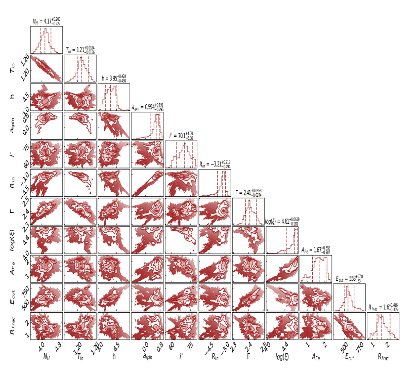
Figure 6: Posterior distribution of the spectral parameters obtained from the MCMC analysis with the RelxillLp model. Plotting was performed using corner (Foreman-Mackey, 2016). Central dashed lines correspond to the peak values whereas $1\sigma$ confidence levels are represented by dashed lines on either side.

Table 4: NuSTAR Spectral Analysis Results

	Powerlaw	Cutoffpl	Nthcomp	RelxillCp	RelxillLp	RelxillLpCp
$n_{\mathrm{H}}$ ($10^{-22}\mathrm{cm^{-2}}$)	$4.63_{-0.28}^{+0.28}$	$4.32_{-0.23}^{+0.27}$	$3.27_{-0.35}^{+0.91}$	$4.05_{-0.03}^{+0.03}$	$4.12_{-0.09}^{+0.09}$	$4.32_{-0.11}^{+0.11}$
$T_{\mathrm{in}}$ (keV)	$1.185_{-0.010}^{+0.015}$	$1.16_{-0.03}^{+0.03}$	$1.149_{-0.009}^{+0.006}$	$1.2358_{-0.0007}^{+0.0007}$	$1.220_{-0.004}^{+0.004}$	$1.211_{-0.005}^{+0.005}$
$\Gamma$	$2.46_{-0.02}^{+0.02}$	$2.24_{-0.08}^{+0.08}$	$2.36_{-0.01}^{+0.02}$	$2.381_{-0.003}^{+0.003}$	$2.421_{-0.004}^{+0.004}$	$2.244_{-0.002}^{+0.002}$
$E_{\mathrm{Fe}}$ (keV)	$6.48_{-0.02}^{+0.02}$	$6.27_{-0.13}^{+0.16}$	$6.40_{-0.02}^{+0.12}$	-	-	-
$\sigma_{\mathrm{Fe}}$ (keV)	$0.50_{-0.05}^{+0.05}$	$0.6_{-0.2}^{+0.3}$	$0.62_{-0.07}^{+0.10}$	-	-	-
normFe ($10^{-3}$)	$3.5_{-0.8}^{+0.4}$	$4.6_{-0.2}^{+5.3}$	$6.0_{-0.8}^{+1.2}$	-	-	-
$E_{\mathrm{Ni}}$ (keV)	$7.99_{-0.03}^{+0.04}$	$8.0_{-0.2}^{+0.3}$	$8.1_{-0.1}^{+0.2}$	-	-	-
$\sigma_{\mathrm{Ni}}$ (keV)	$0.56_{-0.06}^{+0.07}$	$0.5_{-0.2}^{+0.3}$	$0.48_{-0.18}^{+0.12}$	-	-	-
normNi ($10^{-3}$)	$1.7_{-0.6}^{+0.4}$	$1.3_{-1.3}^{+0.9}$	$1.7_{-1.1}^{+1.0}$	-	-	-
$kT_{e}$ (keV)	-	$94_{-39}^{+93}$	$132_{-123}^{+476}$	$400^{f}$	$400^{f}$	$400^{f}$
$R_{\mathrm{refl}}$	-	-	-	$0.67_{-0.06}^{+0.06}$	$0.76_{-0.04}^{+0.04}$	$0.470_{-0.014}^{+0.014}$
$A_{\mathrm{Fe}}$ ($A_{\sun}$)	-	-	-	$0.47_{-0.06}^{+0.06}$	$1.50_{-0.12}^{+0.12}$	$0.44_{-0.04}^{+0.04}$
$a^{*}$	-	-	-	$0.65_{-0.06}^{+0.04}$	$0.70_{-0.31}^{+0.15}$	$0.63_{-0.07}^{+0.07}$
$i$ (∘)	-	-	-	$69.8_{-0.5}^{+0.5}$	$58_{-2}^{+2}$	$37_{-3}^{+3}$
$R_{\mathrm{in}}$ ($R_{\mathrm{ISCO}}$)	-	-	-	$2.2_{-0.6}^{+0.4}$	$2.5_{-0.5}^{+0.5}$	$1.7_{-0.5}^{+1.4}$
$R_{\mathrm{br}}/h$ ($r_{g}$)	-	-	-	$14.3_{-0.6}^{+0.6}$	$3.59_{-0.11}^{+0.15}$	$5.484_{-0.009}^{+0.009}$
$\log\xi$	-	-	-	$3.39_{-0.04}^{+0.04}$	$4.48_{-0.05}^{+0.05}$	$3.01_{-0.02}^{+0.02}$
$q_{1}$	-	-	-	$8.61_{-0.41}^{+0.37}$	-	-
$q_{2}$	-	-	-	$0.35_{-0.11}^{+0.10}$	-	-
normdiskbb	$305_{-21}^{+14}$	$379_{-31}^{+33}$	$464_{-16}^{+21}$	$276_{-6}^{+6}$	$265_{-6}^{+6}$	$299_{-8}^{+8}$
norm	$4.5_{-0.2}^{+0.2}$	$2.9_{-0.5}^{+0.7}$	$0.130_{-0.001}^{+0.002}$	$0.0315_{-0.0008}^{+0.0008}$	$0.0415_{-0.0002}^{+0.0003}$	$0.04694_{-0.00008}^{+0.00008}$
$\chi^{2}$/dof	950/956	907/955	908/955	916/952	940/954	933/954
$\tilde{\chi}^{2}$	0.9936	0.9502	0.9504	0.9618	0.9854	0.9775
$F_{2-10}$ ($10^{-9}$ ergs cm-2 s-1)	$9.656_{-0.01}^{+0.01}$	$9.652_{-0.010}^{+0.010}$	$9.804_{-0.010}^{+0.010}$	$9.824_{-0.010}^{+0.010}$	$9.832_{-0.010}^{+0.010}$	$9.807_{-0.010}^{+0.010}$

^f indicates parameters that were fixed during analysis.

‘norm’ refers to the normalization of the primary model component.

4 Concluding Remarks

We analyzed the Swift J1728.9–3613 data obtained from MAXI/GSC in the form of one-day binned lightcurves, two NICER/XTI observations taken during the rising phase of the outburst, and one NuSTAR/FPMB observation taken near the peak of the outburst. Spectral analysis was performed on the NICER observations in the $0.3-10$ keV range in order to understand the parameters of the system at the beginning of the outburst. We then examined the NuSTAR observation in the $3-78$ keV range to more closely probe the accretion process and to measure parameters such as spin, inner disc radius, and inclination angle.

The long term lightcurve analysis revealed that, in total, Swift J1728.9–3613 devoured roughly 90% of the mass of Mars and released $\sim 5.2\times 10^{44}$ ergs of energy in $2-20$ keV energy band. We also find that lightcurves in various energy bands correlate with each other, where softer photons are delayed compared to their harder counterparts. The maximum delay was observed between the $2-4$ and $10-20$ keV photons with a mean lag of $\tilde{\tau}=(8.4\pm 1.9)$ days. Production of such a delay is likely related to the viscous delay of matter spiraling through the accretion disc during the outburst. This is supported by the presence of a strong multi-color disc component in the NICER spectra during the rising phase, with an increase normalization between the first and second observations.

Various models were used to understand the key parameters involved in the accretion process. In resolving the spectrum of Swift J1728.9–3613 during the primary NuSTAR observation we revealed a sudden decrease in hard emission, with power-law normalization decreasing from $3.3_{-0.5}^{+0.6}$ to $1.54_{-0.07}^{+0.07}$ ph keV^-1 cm^-2. Such a reduction could have have resulted from large amounts of ejecta being carried away from the corona in a relatively short amount of time, so-called blobby jets. These ejections can appear to move at superluminal speeds, and have been definitively reported on in several other outbursting black holes (e.g. Fender et al., 1998; Hjellming & Rupen, 1995). Turning to the time-averaged spectrum, we obtained a hydrogen column density of $4.63^{+0.28}_{-0.28}\times 10^{-22}$ cm^-2 using the WILM (Wilms et al., 2000) abundance from the Tbabs*{Diskbb+Powerlaw} model. Using the ANGR (Anders & Grevesse, 1989) abundance, we found a lower ($2.99^{+0.11}_{-0.11}\times 10^{-22}$ cm^-2) column density for the same model. The disc temperature varied from 1.15 to 1.23 keV across all the models, with Powerlaw yielding an inner temperature of $T_{in}=1.18^{+0.015}_{-0.010}$ keV. From the Nthcomp model, we estimated a coronal electron temperature of $kT_{e}=132^{+476}_{-123}$ keV. The coronal temperature remains unconstrained from our time-averaged spectral analysis. However, when we examined the hardness-resolved spectra using the Cutoffpl model, we found the cutoff temperatures were better constrained, having values $E_{\rm cut}=94_{-34}^{+78}$ keV in region i and $E_{\rm cut}=79_{-18}^{+28}$ keV in region ii. We found signatures of the Fe K$\alpha$ line around $(6.48\pm 0.02)$ keV with an equivalent width of $53$ eV. Apart from the Fe K$\alpha$ line, we also observed an Ni emission line around $(8.0\pm 0.3)$ keV with an equivalent width of $60$ eV. This Ni line has previously been observed in several BHXRBs and AGNs (Corliss & Sugar, 1981; Molendi et al., 2003; Fukazawa et al., 2016; Medvedev et al., 2018). It is possible that the $8.06_{-0.28}^{+0.10}$ keV line is observed due to the blue-shifted wing of the Fe K$\alpha$. However, if this were the case, we would also expect to observe a corresponding redshifted wing at roughly 6.4 - (8 - 6.4) = 4.8 keV (Cui et al., 2000). Given that we detect strong signatures of the emission line at 6.4 keV in the first place and the 8 keV Ni line has been previously identified, we believe that Ni emission line could be the more plausible explanation. Future generation satellites, such as Colibrì, (Heyl et al., 2019; Caiazzo et al., 2019) would be capable of resolving these lines more accurately and locating line emitting regions.

We applied phenomenological models, like Cutoffpl to fit the NuSTAR data and estimate the luminosity of the accretion disc during that observation. Using $L_{2-10}=4\pi D^{2}F_{2-10}$, assuming a distance of 10 kpc, we find $L_{2-10}=1.09\times 10^{38}~{}\rm{erg~{}s^{-1}}$. Assuming a mass-to-radiation conversion efficiency of $\eta=0.1$ based on our measured spin value (Reynolds, 2021), we find a mass accretion rate of $\dot{M}=L/\eta c^{2}=1.2\times 10^{18}~{}\rm{g~{}s^{-1}}$. Using the lower mass limit of Swift J1728.9–3613 reported by Saha et al. (2022), $\sim 5M_{\odot}$ accounting for spin, we estimate $L/L_{\rm Edd}\sim 0.17$ during the observation. Combining this mass with the MAXI/GSC light curves, we find a maximum accretion rate of $L/L_{\rm Edd}\sim 0.28$ during the peak of the outburst.

Three models from the Relxill family were selected for analysis with the NuSTAR data in order to estimate the more complex properties of Swift J1728.9–3613, namely RelxillCp, RelxillLp, and RelxillLpCp. Since RelxillCp assumes that the irradiation of the disc behaves like a broken power-law, this model estimates a steep inner emissivity index of $q_{1}=8.61_{-0.41}^{+0.37}$ that becomes much flatter ($q_{2}=0.35_{-0.11}^{+0.10}$) at the break radius $R_{\rm br}=14.3_{-0.6}^{+0.6}~{}r_{g}$. Otherwise, the three models estimate spin parameters of $0.65_{-0.06}^{+0.04}$, $0.70_{-0.31}^{+0.15}$, and $0.63_{-0.07}^{+0.07}$; inner disc radii of $2.2_{-0.6}^{+0.4}$ $R_{\mathrm{ISCO}}$, $2.5_{-0.5}^{+0.5}~{}R_{\mathrm{ISCO}}$, and $1.7_{-0.5}^{+1.4}~{}R_{\mathrm{ISCO}}$; and inclination angles of $69.8_{-0.5}^{+0.5}$ degrees, $58_{-2}^{+2}$ degrees, and $37_{-3}^{+3}$ degrees, respectively.

Data Availability

We used publicly available archival data of MAXI, NICER and NuSTAR observatories for this work. All the models used in this work, are publicly available. Appropriate links are provided in the text.

References

- Alabarta et al. (2021) Alabarta K., et al., 2021, MNRAS, 507, 5507
- Alexander (2014) Alexander T., 2014, ZDCF: Z-Transformed Discrete Correlation Function, Astrophysics Source Code Library, record ascl:1404.002 (ascl:1404.002)
- Anders & Grevesse (1989) Anders E., Grevesse N., 1989, Geochimica Cosmochimica Acta, 53, 197
- Arnaud (1996) Arnaud K. A., 1996, in Jacoby G. H., Barnes J., eds, Astronomical Society of the Pacific Conference Series Vol. 101, Astronomical Data Analysis Software and Systems V. p. 17
- Barthelmy et al. (2019) Barthelmy S. D., et al., 2019, The Astronomer’s Telegram, 12436, 1
- Bhuvana et al. (2021) Bhuvana G. R., Radhika D., Agrawal V. K., Mandal S., Nandi A., 2021, MNRAS, 501, 5457
- Bright et al. (2019) Bright J., Fender R., Woudt P., Miller-Jones J., 2019, The Astronomer’s Telegram, 12522, 1
- Caiazzo et al. (2019) Caiazzo I., et al., 2019, Unveiling the secrets of black holes and neutron stars with high-throughput, high-energy resolution X-ray spectroscopy, doi:10.5281/zenodo.3824441, https://doi.org/10.5281/zenodo.3824441
- Casares & Jonker (2014) Casares J., Jonker P. G., 2014, Space Sci. Rev., 183, 223
- Chakrabarti & Titarchuk (1995) Chakrabarti S., Titarchuk L. G., 1995, ApJ, 455, 623
- Chan et al. (2013) Chan C.-k., Psaltis D., Özel F., 2013, ApJ, 777, 13
- Chatterjee et al. (2020) Chatterjee A., Dutta B. G., Nandi P., Chakrabarti S. K., 2020, MNRAS, 497, 4222
- Churazov et al. (2001) Churazov E., Gilfanov M., Revnivtsev M., 2001, MNRAS, 321, 759
- Connors et al. (2022) Connors R. M. T., et al., 2022, ApJ, 935, 118
- Corliss & Sugar (1981) Corliss C., Sugar J., 1981, Journal of Physical and Chemical Reference Data, 10, 197
- Corral-Santana et al. (2016) Corral-Santana J. M., Casares J., Muñoz-Darias T., Bauer F. E., Martínez-Pais I. G., Russell D. M., 2016, A&A, 587, A61
- Cui et al. (2000) Cui W., Chen W., Zhang S. N., 2000, ApJ, 529, 952
- Dauser et al. (2014) Dauser T., Garcia J., Parker M. L., Fabian A. C., Wilms J., 2014, MNRAS, 444, L100
- Dauser et al. (2016) Dauser T., García J., Walton D. J., Eikmann W., Kallman T., McClintock J., Wilms J., 2016, A&A, 590, A76
- Done et al. (2007) Done C., Gierliński M., Kubota A., 2007, A&ARv, 15, 1
- Draghis et al. (2021) Draghis P. A., Miller J. M., Zoghbi A., Kammoun E. S., Reynolds M. T., Tomsick J. A., 2021, ApJ, 920, 88
- Draghis et al. (2022) Draghis P. A., Miller J. M., Zoghbi A., Reynolds M., Costantini E., Gallo L. C., Tomsick J. A., 2022, arXiv e-prints, p. arXiv:2210.02479
- Ducci et al. (2019) Ducci L., et al., 2019, The Astronomer’s Telegram, 12502, 1
- Enoto et al. (2019) Enoto T., et al., 2019, The Astronomer’s Telegram, 12455, 1
- Event Horizon Telescope Collaboration et al. (2019) Event Horizon Telescope Collaboration et al., 2019, ApJ, 875, L1
- Event Horizon Telescope Collaboration et al. (2022) Event Horizon Telescope Collaboration et al., 2022, ApJ, 930, L12
- Fabian et al. (1989) Fabian A. C., Rees M. J., Stella L., White N. E., 1989, MNRAS, 238, 729
- Fabian et al. (2015) Fabian A. C., Lohfink A., Kara E., Parker M. L., Vasudevan R., Reynolds C. S., 2015, MNRAS, 451, 4375
- Fender et al. (1998) Fender R. P., Garrington S. T., Mckay D. J., Muxlow T. W. B., Pooley G. G., Spencer R. E., Stirling A. M., Waltman E. B., 1998, Mon. Not. R. Astron. Soc, 000, 0
- Foreman-Mackey (2016) Foreman-Mackey D., 2016, The Journal of Open Source Software, 1, 24
- Fukazawa et al. (2016) Fukazawa Y., Furui S., Hayashi K., Ohno M., Hiragi K., Noda H., 2016, ApJ, 821, 15
- Garain et al. (2012) Garain S. K., Ghosh H., Chakrabarti S. K., 2012, ApJ, 758, 114
- Garain et al. (2014) Garain S. K., Ghosh H., Chakrabarti S. K., 2014, MNRAS, 437, 1329
- García & Kallman (2010) García J., Kallman T. R., 2010, ApJ, 718, 695
- García et al. (2013) García J., Dauser T., Reynolds C. S., Kallman T. R., McClintock J. E., Wilms J., Eikmann W., 2013, ApJ, 768, 146
- García et al. (2014) García J., et al., 2014, ApJ, 782, 76
- García et al. (2018) García J. A., et al., 2018, ApJ, 864, 25
- García et al. (2019) García J. A., et al., 2019, ApJ, 885, 48
- Gendreau et al. (2012) Gendreau K. C., Arzoumanian Z., Okajima T., 2012, in Takahashi T., Murray S. S., den Herder J.-W. A., eds, Society of Photo-Optical Instrumentation Engineers (SPIE) Conference Series Vol. 8443, Space Telescopes and Instrumentation 2012: Ultraviolet to Gamma Ray. p. 844313, doi:10.1117/12.926396
- George & Fabian (1991) George I. M., Fabian A. C., 1991, MNRAS, 249, 352
- Gou et al. (2009) Gou L., et al., 2009, ApJ, 701, 1076
- Harrison et al. (2013) Harrison F. A., et al., 2013, ApJ, 770, 103
- Heyl et al. (2019) Heyl J., et al., 2019, in Bulletin of the American Astronomical Society. p. 175
- Hjellming & Rupen (1995) Hjellming R. M., Rupen M. P., 1995, Nature, 375, 464
- Homan et al. (2001) Homan J., Wijnands R., van der Klis M., Belloni T., van Paradijs J., Klein-Wolt M., Fender R., Méndez M., 2001, ApJS, 132, 377
- Horne (1985) Horne K., 1985, MNRAS, 213, 129
- Hu et al. (2019) Hu Y. D., et al., 2019, The Astronomer’s Telegram, 12443, 1
- Ingram et al. (2009) Ingram A., Done C., Fragile P. C., 2009, MNRAS, 397, L101
- Jana et al. (2021a) Jana A., Naik S., Chatterjee D., Jaisawal G. K., 2021a, MNRAS, 507, 4779
- Jana et al. (2021b) Jana A., et al., 2021b, Research in Astronomy and Astrophysics, in Press.,
- Jana et al. (2022) Jana A., Naik S., Jaisawal G. K., Chhotaray B., Kumari N., Gupta S., 2022, MNRAS, 511, 3922
- Kreidberg et al. (2012) Kreidberg L., Bailyn C. D., Farr W. M., Kalogera V., 2012, ApJ, 757, 36
- Kubota et al. (1998) Kubota A., Tanaka Y., Makishima K., Ueda Y., Dotani T., Inoue H., Yamaoka K., 1998, PASJ, 50, 667
- Li et al. (2005) Li L.-X., Zimmerman E. R., Narayan R., McClintock J. E., 2005, ApJS, 157, 335
- Luminet (1979) Luminet J. P., 1979, A&A, 75, 228
- Magdziarz & Zdziarski (1995) Magdziarz P., Zdziarski A. A., 1995, MNRAS, 273, 837
- Mastroserio et al. (2019) Mastroserio G., Ingram A., van der Klis M., 2019, MNRAS, 488, 348
- Matsuoka et al. (2009) Matsuoka M., et al., 2009, PASJ, 61, 999
- McClintock et al. (2006) McClintock J. E., Shafee R., Narayan R., Remillard R. A., Davis S. W., Li L.-X., 2006, ApJ, 652, 518
- Medvedev et al. (2018) Medvedev P. S., Khabibullin I. I., Sazonov S. Y., Churazov E. M., Tsygankov S. S., 2018, Astronomy Letters, 44, 390
- Miller et al. (2012) Miller J. M., et al., 2012, ApJ, 759, L6
- Miller et al. (2018) Miller J. M., et al., 2018, ApJ, 860, L28
- Miniutti & Fabian (2004) Miniutti G., Fabian A. C., 2004, MNRAS, 349, 1435
- Molendi et al. (2003) Molendi S., Bianchi S., Matt G., 2003, MNRAS, 343, L1
- Mudambi et al. (2020) Mudambi S. P., Rao A., Gudennavar S. B., Misra R., Bubbly S. G., 2020, MNRAS, 498, 4404
- Negoro et al. (2019) Negoro H., et al., 2019, The Astronomer’s Telegram, 13256, 1
- Novikov & Thorne (1973) Novikov I. D., Thorne K. S., 1973, in Black Holes (Les Astres Occlus). pp 343–450
- Remillard & McClintock (2006) Remillard R. A., McClintock J. E., 2006, ARA&A, 44, 49
- Reynolds (2021) Reynolds C. S., 2021, ARA&A, 59, 117
- Saha et al. (2022) Saha D., Mandal M., Pal S., 2022, arXiv e-prints, p. arXiv:2210.13748
- Shakura & Sunyaev (1973) Shakura N. I., Sunyaev R. A., 1973, A&A, 500, 33
- Shaposhnikov & Titarchuk (2007) Shaposhnikov N., Titarchuk L., 2007, ApJ, 663, 445
- Smith et al. (2002) Smith D. M., Heindl W. A., Swank J. H., 2002, ApJ, 569, 362
- Sreehari et al. (2019) Sreehari H., Ravishankar B. T., Iyer N., Agrawal V. K., Katoch T. B., Mandal S., Nandi A., 2019, MNRAS, 487, 928
- Sreehari et al. (2020) Sreehari H., Nandi A., Das S., Agrawal V. K., Mandal S., Ramadevi M. C., Katoch T., 2020, MNRAS, 499, 5891
- Steiner et al. (2009) Steiner J. F., Narayan R., McClintock J. E., Ebisawa K., 2009, PASP, 121, 1279
- Steiner et al. (2014) Steiner J. F., McClintock J. E., Orosz J. A., Remillard R. A., Bailyn C. D., Kolehmainen M., Straub O., 2014, ApJ, 793, L29
- Sunyaev & Titarchuk (1980) Sunyaev R. A., Titarchuk L. G., 1980, A&A, 500, 167
- Sunyaev & Titarchuk (1985) Sunyaev R. A., Titarchuk L. G., 1985, A&A, 143, 374
- Taylor et al. (2003) Taylor R. D., Uttley P., McHardy I. M., 2003, MNRAS, 342, L31
- Tetarenko et al. (2016) Tetarenko B. E., Sivakoff G. R., Heinke C. O., Gladstone J. C., 2016, ApJS, 222, 15
- Tomsick et al. (2018) Tomsick J. A., et al., 2018, ApJ, 855, 3
- Torres et al. (2019) Torres M. A. P., Casares J., Jiménez-Ibarra F., Muñoz-Darias T., Armas Padilla M., Jonker P. G., Heida M., 2019, ApJ, 882, L21
- Uttley et al., (2020) Uttley et al., P., 2020, in Society of Photo-Optical Instrumentation Engineers (SPIE) Conference Series. p. 114441E, doi:10.1117/12.2562523
- Verner et al. (1996) Verner D. A., Ferland G. J., Korista K. T., Yakovlev D. G., 1996, ApJ, 465, 487
- Viergutz (1993) Viergutz S. U., 1993, A&A, 272, 355
- Wilms et al. (2000) Wilms J., Allen A., McCray R., 2000, ApJ, 542, 914
- Xu et al. (2020) Xu Y., Harrison F. A., Tomsick J. A., Walton D. J., Barret D., García J. A., Hare J., Parker M. L., 2020, ApJ, 893, 30
- Zdziarski & Marco (2020) Zdziarski A. A., Marco B. D., 2020, The Astrophysical Journal, 896, L36
- Zdziarski et al. (1996) Zdziarski A. A., Johnson W. N., Magdziarz P., 1996, MNRAS, 283, 193
- Zhang et al. (1997) Zhang S. N., Cui W., Chen W., 1997, ApJ, 482, L155
- Zhao et al. (2021) Zhao X., et al., 2021, ApJ, 916, 108
- Życki et al. (1999) Życki P. T., Done C., Smith D. A., 1999, MNRAS, 309, 561
- den Hartog et al. (2020) den Hartog R. H., Uttley P., Willingale R., Hoevers H., den Herder J.-W., Wise M., 2020, in den Herder J.-W. A., Nakazawa K., Nikzad S., eds, Space Telescopes and Instrumentation 2020: Ultraviolet to Gamma Ray. SPIE, doi:10.1117/12.2562831, https://doi.org/10.1117%2F12.2562831