Neutral Diversity in Experimental Metapopulations

Abstract

New automated and high-throughput methods allow the manipulation and selection of numerous bacterial populations. In this manuscript we are interested in the neutral diversity patterns that emerge from such a setup in which many bacterial populations are grown in parallel serial transfers, in some cases with population-wide extinction and splitting events. We model bacterial growth by a birth-death process and use the theory of coalescent point processes. We show that there is a dilution factor that optimises the expected amount of neutral diversity for a given amount of cycles, and study the power law behaviour of the mutation frequency spectrum for different experimental regimes. We also explore how neutral variation diverges between two recently split populations by establishing a new formula for the expected number of shared and private mutations. Finally, we show the interest of such a setup to select a phenotype of interest that requires multiple mutations.

Keywords Neutral diversity  $\cdot$ Population genetics  $\cdot$ Experimental evolution

1 Introduction

Experimental evolution is the study of evolutionary dynamics happening in real time as a response to conditions imposed by the experimenter (Kawecki et al.,, 2012). Microbial populations are widely used because they offer numerous experimental advantages: large population sizes, easily manipulable environments, possibility to freeze and store whole populations indefinitely… Experimental evolution requires the set-up of many parallel bacterial cultures that can take several forms from bottles ($\approx 10^{1}L$) to tubes ($\approx 10^{-3}L$), microplates ($\approx 10^{-4}$L), or microfluidic compartments ($\approx 10^{-9}L$).

Recently, new techniques for the high-throughput manipulation of bacterial populations have emerged. For instance, digital millifluidics (Cottinet,, 2013; Dupin,, 2018; Doulcier,, 2019) allows the possibility of producing and imaging thousands of droplets of culture broth within a carrying fluid. The droplets amount to around $2\times 10^{-6}L$ with a carrying capacity of $10^{5}$ to $10^{6}$ cells (Cottinet,, 2013). Droplets can be imaged and quantitative measures be performed (optical density, fluorescence signal…) during growth of the bacteria, allowing a high-throughput monitoring of ecological dynamics.

Nested populations in which both particles (bacterial cells) and collectives (bacterial populations) are individuals with their own birth and death events can be readily implemented in experimental microbiology. For instance, such experiments are routinely performed in microcosms (Hammerschmidt et al.,, 2014). However, the ability of millifluidic devices to monitor in the order of a thousand of cultures and retrieve some of them for analysis makes them particularly suitable for the artificial selection of microbial communities (Xie and Shou,, 2021) for instance, through ecological scaffolding (Doulcier et al.,, 2020; Black et al.,, 2020).

Neutral diversity in experimentally nested populations is the focus of this manuscript. The aim is to build a quantitative understanding of simple diversity patterns within the experimental setup. First, a model of the device is presented. It relies on the assumption that cells are in constant exponential growth. The optimal operating regime parameters of the machine (dilution ratio, duration of collective growth cycles, carrying capacity…) are derived from characteristics of the biological material: birth and death rates. From a theoretical perspective, the system constitutes a dynamical meta-population in discrete space with explicit demography. It contrasts with simpler models in which demography is simplified (Etheridge,, 2008), as well as with more complex spatially structured models (Barton et al.,, 2002, 2013) in which space is continuous. Second, a coalescent model of the population across bottlenecks is proposed and coupled to a neutral mutation model with infinite alleles. This allows computation of the number of mutations, and the distribution of allele frequencies within droplets after several collective growth cycles. It shows that small bottlenecks are required to maximise diversity in one cycle, but larger bottlenecks are more favourable for diversification across many cycles. The speed at which diversity accumulates decreases with time. Then, the effect of splitting a droplet into several lineages is studied by computing the number of mutations accumulated in a single, or all the droplet lineages. Finally, a simple mutation accumulation model illustrates the interest of droplet-level selection for artificial selection.

2 Modelling Nested Population Dynamics

Consider a device that allows the manipulation of collectives of Darwinian particles via serial transfers (Figure 1). Cells (called particles) are distributed among a train of $D$ droplets (called populations, or collectives). The birth and death of cells are modelled by a linear branching process with constant rates $b$ for birth and $d$ for death. The net growth rate $r:=b-d$ is called the Malthusian parameter. After a duration $T$, a new train of $D$ droplets is prepared by diluting them $\frac{1}{\delta}$ fold. Hence, for each dilution event, a cell has a probability $\delta$ of being sampled and thus being present in the new droplet. This procedure is repeated periodically, each dilution followed by a growth phase constitutes a cycle of the experiment or a collective generation.

More formally, the initial population contains $Z_{0}=c$ cells, and is submitted to a bottleneck with sampling probability $\delta$ at the beginning of every cycle except the first, meaning that bottlenecks occur at times $T,2T\ldots nT$. The $n$th cycle corresponds to the slice of time $[(n-1)T,nT)$. Thus, "the end of cycle n" correspond to the moment $nT^{-}$, just before the $n$th dilution. To illustrate, at the end of the third cycle, $t=3T^{-}$, and the population has experienced two bottlenecks at time $T$ and $2T$.

Birth $b$ and death $d$ rates depend on the biological material used (species, strain…) as well as the culture medium and are not easily controlled. However, the duration of the growth phase $T$, the dilution factor $\delta$ and the number of collectives $D$ can be changed by altering the experimental setup. A model can help predict the effect of those parameters and find the ones that should be the focus of engineering efforts.

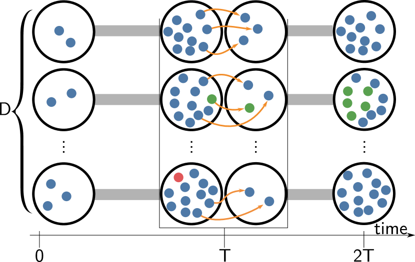
Figure 1: Sketch of the experimental setup. Darwinian particles following a birth-death process with rates $b,d$ are distributed in collectives within $D$ droplets. After a growth phase duration $T$, a new cycle starts: the content of each droplet is diluted to seed a new droplet. Each particle has a probability $\delta$ to be transferred at the start of the next cycle. Here the serial transfer regime is depicted: each droplet is diluted into exactly a single new droplet in the next cycle. In the full nested population design, a droplet can be split in several droplets in the cycle, or removed altogether.

Table 1: Parameter names and symbols reference

	Collective-level parameters		Particle-level parameters
$D$	Population size	$b$	Birth rate
$T$	Cycle duration	$d$	Death rate
$n$	Number of cycles	$r$	Malthusian parameter (b-d)
$K$	Carrying capacity	$\delta$	Survival probability (at a bottleneck)
$c$	Initial number of particles	$\theta$	Mutation rate

2.1 Optimal Operating Regime

When designing a serial transfer experiment, the operator has three main parameters that might be controlled: the size of the cultures (and by extension the carrying capacity of the particles $K$), the duration of the growth phase separating two successive transfers $T$, and the dilution rate $\delta$. Two problems must be avoided: if population sizes are too small and dilution too high, the resulting cultures might be empty. Conversely, if the population sizes are too large, and dilution too low, the population will spend most of its time in stationary phase, with little effect of bottlenecks.

Any dilution event presents the risk of extinguishing the population. When performing a serial transfer experiment, this must be avoided at all cost because an empty microcosm signs the end of the experiment (at least for the given independent lineage). In a nested population design, the presence of some empty microcosms can be tolerated because empty niches in the population can be filled by splitting a single parent droplet into several offspring droplets in the next generation.

Stationary phase is in general not desirable for several reasons. First, a population that reaches saturation will go through fewer generations than if it was growing freely, reducing the potential evolutionary dynamics. Moreover, physiological changes in stationary phase might result in undesired phenotypic effects on the population. Finally, in the case of millifluidic experiments, saturating densities are known to increase the risk of cross-contamination between droplets.

For all these reasons, there is an optimal dilution rate, that keeps the population in exponential phase while maximising the population size, at which selection experiments should be conducted.

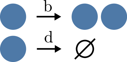
Figure 2: Events in a Linear-Birth-Death Model. Individuals give birth to new individuals at a constant rate $b$, and die at constant rate $d$, independently. The process is super-critical if $b>d$.

A model of population dynamics can provide a first estimate of the optimal range of parameters for an experiment. In the following, a stochastic model of particles in exponential growth conditions (i.e., super-critical) with periodic bottlenecks is used to derive the probability of losing a single particle lineage, or a single collective lineage due to the effect of dilution, as a function of experimentally accessible parameters. Saturation phenomena are not modelled explicitly as the birth and death rates are considered independent of population size, but the population dynamics are required to stay under a carrying capacity threshold.

Figure 3: Dilution process. Individual particles are independently selected to be transferred to the next cycle (with probability $\delta$) or sent to the waste (with probability $1-\delta$).

2.1.1 Survival of a single lineage

A first quantity that can be derived from the linear branching process with periodic dilution that models the population dynamics is the probability that a single initial particle has no descent in the population after $n$ cycles.

Proposition 1 (Survival Probability)

Cells within droplets in serial transfers are modelled by a linear birth-death process with constant parameters $b$ and $d$, that is subject to periodic bottlenecks every duration $T$.

Let $s_{n}$ be the probability that a lineage spawned by a single cell is not extinct at the end of the $n$th cycle. Then,

$$s_{n}= 1-h_{Q_{0}Q^{n-1}}(0)$$

Where $h_{A}$ is the linear fractional function with coefficient $A$:

$$h_{\begin{bmatrix}a&b\\ c&d\end{bmatrix}}(s)=\frac{as+b}{cs+d}$$ (1)

And the matrices $Q_{0}$ and $Q$ are:

$$Q_{0}=\begin{bmatrix}\delta(p-q)&q\\ \delta(p-1)&1\end{bmatrix};\;\;\;Q=\begin{bmatrix}p-(1-\delta)-\delta q&(1-\delta)+\delta q\\ p-1&1\end{bmatrix}$$

with,

		$p(b,d,T)$	$q(b,d,T)$
Subcritical particles	$b<d$	$\frac{-r}{d-be^{rT}}$	$\frac{d(1-e^{rT})}{d-be^{rT}}$
Critical particles	$b=d$	$\frac{1}{1+bT}$	$\frac{bT}{1+bT}$
Supercritical particles	$b>d$	$\frac{re^{-rT}}{b-de^{-rT}}$	$\frac{d(1-e^{-rT})}{b-de^{-rT}}$

(Proof page 1.)

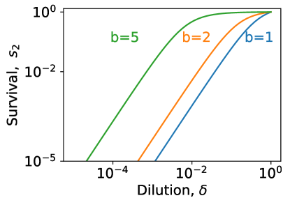
Figure 4: Survival probability at the end of the second cycle $s_{2}$. This corresponds to a first growth phase, a dilution event, and a second growth phase. The probability is presented as a function of the dilution rate $\delta$ for pure birth processes $b>0,d=0,T=1$.

Proposition 1 shows that the survival probability of a lineage depends on the birth $b$ and death $d$ rates of the cells, but is also a function of the dilution rate $\delta$, duration of the growth phase $T$ and the number of cycles $n$. When considering a single dilution and a pure-birth process ($s_{2}$, Figure 4), the survival probability is equivalent to $\delta\mathbb{E}(Z_{T})$ when $\delta$ is small, hence the linear increase with slope $1$ in log-log scale.

The numerical computation of $Q^{n}$ might be problematic because of repeated multiplication of the small numbers. However, since the final result only involves the ratio $Q^{n}_{01}/Q^{n}_{11}$, it is possible to normalise $Q$ to have its smallest value being $1$. Indeed, this ratio does not depend on a multiplicative scalar on the matrix: $\forall\alpha>0$, $h_{Q^{n}}(0)=h_{\alpha Q^{n}}(0)$. Taking $\alpha=\frac{1}{\delta}$ greatly improves the numerical stability of the computation.

The limit of this probability when the number of cycles increases gives a clearer understanding of the long term behaviour of the population:

Proposition 2 (Long Term Survival Probability)

Let $s_{n}$ be the survival probability after $n$ cycles of the lineage spawned by a single cell.

$$\lim\limits_{n\to+\infty}s_{n}=\begin{cases}0&\text{if }\delta e^{rT}\leq 1\\ \frac{r(\delta-e^{-rT})}{\delta b(1-e^{-rT})}&\text{otherwise.}\end{cases}$$

(Proof page 2.)

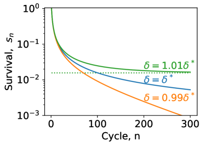
Figure 5: Survival probability for several cycles $s_{n}$. The probability is presented for pure birth processes $b=1,d=0,T=1$. Above the critical threshold $\delta^{*}$, the survival probability does not tend toward $0$. The dotted line corresponds to the limit $s_{\infty}$.

Proposition 2 confirms that, in the long run, lineages go extinct with certainty ($s_{\infty}=0$) if and only if the expected number $\delta e^{rT}$ of cells descending from a single initial cell and surviving the first bottleneck is smaller than $1$. It gives the survival probability otherwise (see Figure 5).

In the following, only super-critical populations will be considered $(b>d)$.

2.1.2 Optimal cycle duration and dilution

Saturation of particle dynamics is not desirable, as mentioned earlier. Depending on the nature of the particles (species, strain), and of the medium (pH, nutrient availability, temperature), it is possible to define an experimental carrying capacity $K$ that corresponds to the number of cells that can be sustained in a droplet without saturation. The simple linear-birth-death model cannot represent saturating populations because no density dependence is included in this model, thus for the model to be coherent, the duration of the growth phase must be short enough that the population size does not reach the carrying capacity:

Proposition 3 (Maximal Cycle Duration)

Let $T^{*}$ be the maximal cycle duration before reaching saturation. Cells are following a supercritical birth-death process with growth rate $b-d=r>0$, The carrying capacity is $K$ and the initial number of cells is $c$ :

$$T^{*}=-\frac{\ln(\frac{c}{K})}{r}$$ (2)

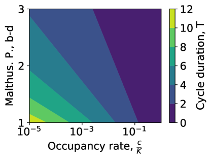
Figure 6: Maximal Cycle Duration $T^{*}$ as a function of the Malthusian parameter $b-d$ and the initial occupancy $\frac{c}{K}$.

Proposition 3 shows that the optimal duration of the growth phase is linear with the inverse of the Malthusian parameter $r$ of the population (Figure 6), meaning that a population that grows (on average) twice as fast as another should be subject to cycles half as long as the other, for a given initial occupancy $\frac{c}{K}$.

Additionally, the optimal duration of the growth phase is proportional to the logarithm of the initial occupancy $\frac{c}{K}$ of the droplet (with a minus sign, since this logarithm is always negative or zero as $c\leq K$). As a consequence, for a given strain, multiplying the volume of the droplets by two, or dividing the inoculum size by two will increase the maximal duration of the growth phase by $\frac{\ln{2}}{r}$.

To keep the same maximal duration $T^{*}$ if the Malthusian parameter $r$ is doubled, the carrying capacity of the droplet must be multiplied by the inverse of the previous initial occupancy $K/c$.

This result holds for a single cycle only. For a given dilution rate $\delta$, the population is shrunk by an expected ratio $\delta$, while for a given cycle duration $T$, the population is expanded by an expected ratio $\delta e^{rT}$. In order to prevent the population from saturating for all cycles, the initial occupancy at the beginning of each cycle must be constant. This consideration allows discovery of the optimal dilution rate when the growth phase duration is fixed:

Proposition 4 (Optimal Dilution Rate)

Let $\delta^{*}$ be the optimal dilution rate for which the expected number of cells is constant across generations. For cells following a birth-death process with growth rate $b-d=r>0$ and a growth phase duration $T$:

$$\delta^{*}=e^{-rT}$$ (3)

If $T=T^{*}$ (Proposition 3),

$$\delta^{*}=\frac{c}{K}$$ (4)

(Proof page 3.)

Proposition 4 shows that the dilution sampling probability should be equal to the initial occupancy when the duration of the cycle is maximal.

To summarise, the optimal operating regime of the experiment can be expressed from the Malthusian parameter of the population and the initial occupancy of the particles $\frac{c}{K}$. As a result, the dilution sampling probability is $\delta^{*}=\frac{c}{K}$ and duration of a cycle is $T^{*}=-\frac{\log(\delta^{*})}{r}$. Fixing any two of $(c,K,T,\delta)$ values constrains the other two.

When the experiment is in the optimal regime, the expression of the survival of a lineage at cycle $n$ is simpler:

Proposition 5 (Optimal Regime Survival Rate)

Let $s_{n}^{*}$ be the survival probability of a lineage after $n$ cycles of duration $T$ and with bottleneck $\delta^{*}=e^{-rT}$, where $r=b-d>0$ is the Malthusian parameter of the population.

Then,

$$s_{n}^{*}=\frac{r}{bn(1-\delta)+\delta r}$$ (5)

(Proof page 4.)

In the optimal regime, each initial cell has on average one descendant cell surviving the next bottleneck. The process counting the number of cells at time $kT$ is thus a critical Galton–Watson process (as a function of $k$). Proposition 5 shows that, in the optimal regime, the survival probability of a lineage decreases as the inverse of the number of cycles, which is typical of critically branching populations.

Additionally, when taking a finite number of cycles $n$, the survival does not tend toward zero even for vanishingly small bottlenecks $\delta$. This derives from the fact that, in the optimal regime, a small bottleneck is compensated by a long cycle duration $T^{*}$, so vanishingly small bottlenecks correspond to infinitely long cycles.

Finally, in the case of pure-birth (i.e., $d=0$), the survival of a lineage is independent from the birth rate $b$. It is certain if there is no bottleneck ($\delta=1$), and tends toward $\frac{1}{n}$ for vanishingly small bottlenecks ($\delta\to 0$).

Overall, once the size of the droplets (which constrains $K$) and the initial occupancy (which constrains $c$) have been chosen by the operator, other parameters of the machine (duration of the growth phase $T$, dilution rate $\delta$) can be deduced —and conversely, fixing $T$ and $\delta$ constrains $K$ and $c$. The next section explores how should one select these parameters when the aim is to maximise genetic diversity within and between the droplets.

3 Modelling Neutral Diversity

Neutral diversity concerns mutations arising in the population of cells that are assumed to not change their birth or death rates. Neutral diversity gives rise to recognisable patterns that can be predicted from a mechanistic model of birth-death in the population. In experimental evolution, and a fortiori in artificial selection, it is desirable to increase the diversity within the population because it allows greater exploration of the phenotypic space. Indeed, mutations that are essentially neutral for cells might present an interest for the experimenter, or be intermediate states toward new phenotypes.

In the following, mutations follow a Poisson Point Process with constant rate $\theta$ over the lifespan of the cells, independently of their genealogy. As a consequence, the time between two mutations along a lineage (regardless of births and deaths) is exponentially distributed, and thus has no memory: the conditional expected time to the next mutation will be the same for all cells, irrespective of their age or the time of the last mutation in the lineage. This is a simplifying assumption that represents the spontaneous nature of mutations, while ignoring the existence of mutations that can change the mutation rate (Sniegowski et al.,, 1997, 2000).

3.1 Coalescence times and the Coalescent Point Process

The linear branching process (with constant birth rate $b$ and death rate $d$) yields the full genealogy of the population (Figure 8, left). However, the standing diversity at a given time in the population is affected (i) neither by the mutations occurring on lineages that do not have extant individuals (because their mutations have been lost), (ii) nor by mutations that are ancestral to the whole population (because they are shared by all individuals in the population). It is thus sufficient, to characterise the standing diversity, to have the knowledge of the coalescent tree of the population (Figure 8, right), which is the genealogy of the extant individuals up to their most recent common ancestor.

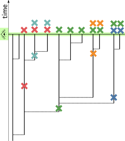
Figure 7: Neutral mutations over the coalescent tree. The neutral mutations (coloured crosses) are distributed following a Poisson Process over the (real) coalescent tree (black). Each individual may carry several mutations distinguishing it from the most recent common ancestor.

Coalescent Point Processes (CPP) are stochastic processes whose realisations are real trees with the same probability as the coalescent tree of the corresponding branching process (Popovic,, 2004; Lambert and Stadler,, 2013). A CPP is defined by a time horizon $t$ and a node depth distribution $f_{H}$. The CPP is the sequence of independent and identically distributed variables $(H_{i})_{i=1\ldots N}$ following $f_{H}$ and stopped at the first element $N$ such that $H_{N}>t$. Usually, the node depth distribution is expressed in the form of the inverse tail distribution $F$:

$$F(t):=\frac{1}{P(H>t)}$$ (6)

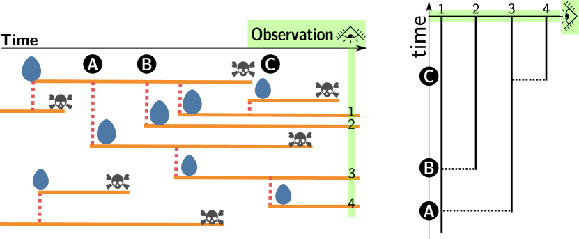
Figure 8: From Birth-Death Process to Coalescent Point Process. On the left-hand side is a birth-death process where a number of individuals give birth (eggs) and die (skulls) at different points in time, which flows from left to right. On the right-hand side is the corresponding continuous coalescent tree, where time flows from bottom to top. Note that at time $C$, lineage $3$ coalesces with lineage $4$ and that at time $B$, lineages $1$ and $2$ coalesce. Finally, at time $A$, lineage $(1,2)$ coalesces with lineage $(3,4)$.

3.2 Measuring neutral diversity

Neutral mutations do not affect the genealogy and can thus be superimposed a posteriori on the coalescent tree. Consider that mutations appear following a Poisson point process with constant rate $\theta$ over the coalescent tree. Thus, a mutation is a point on the coalescent tree, as illustrated in Figure 7. Additionally, assume that reverse mutations are impossible (an assumption referred to as the “infinite sites model”), so that all individual standing above the mutation in the coalescent tree (i.e., the descent of the mutation point) share the mutation (crosses at the top of Figure 7). Individuals may carry zero, one or several mutations.

The mutational richness of the population $M$ (or total diversity) is the number of unique mutations found in the population. Its expected value is proportional to the length of the coalescent tree.

The mutation frequency spectrum $(a_{k})_{k\in\mathbb{N}}$ is another measure of diversity that counts how many mutations are represented by $k$ individuals in the population.

All these measures require some knowledge of the shape of the coalescent tree of the population. The next paragraph is dedicated to establishing this for the simple case of serial transfer, while the next section is dedicated to the case of splitting droplets.

3.3 Diversity Within Droplets in Serial Transfer

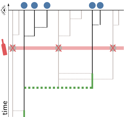
Figure 9: Bottlenecks are modelled by thinning the process. A bottleneck at some point in the past (red bottle) results in the extinction of some lineages (in grey), which modifies the genealogy (thick green lines).

Establishing the law of the Coalescent Point Process of a lineage within serial transfer requires identification of the law of the branch length. This law is well-known for simple branching process such as the Linear Birth-Death process with parameters $(b,d)$ modelling the population dynamics (Lambert and Stadler, (2013), Proposition 5).

The addition of repeated bottlenecks with period $T$ is also possible within the theory ((Lambert and Stadler,, 2013), Proposition 7) by thinning the original process (Figure 9). Each bottleneck at time $iT$, $i=1,\ldots,n$ may remove independently each branch of the CPP with probability ($1-\delta$) (in grey in Figure 9). Removing a branch in the past (at time $iT$) may result in removing several branches in the present, and requires an adjustment to branch length (green in Figure 9). The number of branches removed, and the adjustment to the branch length distribution can be computed from the law of the branch length of the CPP in the absence of bottleneck, the sampling probability $\delta$ and the period of the bottleneck $T$. As a result:

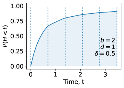
Figure 10: Cumulative probability for the branch length. Dotted lines represent bottlenecks.

Proposition 6 (Coalescent tree of a lineage)

Let $\mathcal{T}_{n}$ be the random coalescent tree spawned by a single particle with extant descent at the end of the $n$th cycle. Then $\mathcal{T}_{n}$ is a Coalescent Point Process (CPP) stopped in $nT$, with inverse tail distribution $F$, and in the case of critical dilution ($\delta^{*}=e^{-rT}$), we have:

$$\forall t=kT+s\in[(n-1)T,nT],F(t)=1+\frac{b}{r}\left(e^{rs}-1+k(e^{rT}-1)\right)$$ (7)

With $k\in\mathbb{N}$ and $s<T$.

(Proof page 5.)

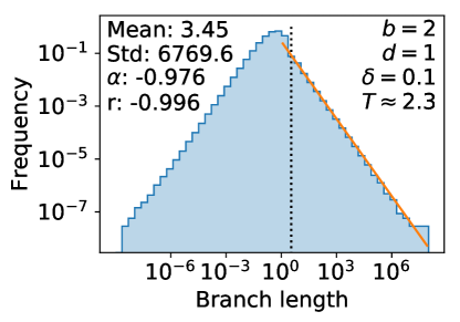
Figure 11: Node depth distribution. Sample of $10^{8}$ realisations of the random variable by the inversion of the cumulative probability function method. Deep nodes follow a power law distribution with parameter $\alpha=-1$ (orange line).

Proposition 6 gives the cumulative probability function for the node depth $H$: $\mathbb{P}(H<t)=1-\frac{1}{F(t)}$ (Figure 10). Note that this function is defined by parts for each cycle.

Because $F(t)\to\infty$ as $t\to\infty$, the cumulative distribution function of node depths tends to 1, which shows that $H$ cannot take the value $+\infty$, as is expected for critically (and also supercritically) branching populations.

The random variable $H$ can be easily sampled from its cumulative probability function. As illustrated in Figure 11, the distribution of deep nodes (deeper than depth $1$) can be fitted by a power law with parameter $-1$ (criticality).

3.4 Number of mutations

In order to find the expected number of mutations within a droplet, the expected size of the full coalescent tree must be considered. This relies on the node depth distribution, conditioned to be lower than the duration of the experiment. It results in the following:

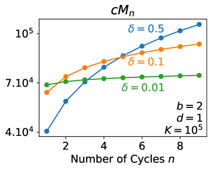
Figure 12: Expected number of mutations through experimental cycles. The expected number of mutations increases with the number of experimental cycles. The initial number of cells is $c=K\delta$. For one cycle ($n=1$), larger bottlenecks give better results (The curve $\delta=0.5$ is higher than the curve for $\delta=0.001$). For more cycles however, larger bottlenecks yield more mutations.

Proposition 7 (Number of mutations)

Let $M_{n}$ be the expected number of mutations (compared to the ancestral phenotype) accumulated in a lineage at the end of the $n$th cycle, with dilution $\delta^{*}=e^{-(b-d)T}$, birth rate of cells $b$, death rate $d$, and mutation rate $\theta$.

$$M_{n}=\theta s_{n}L_{n}$$ (8)

With $L_{n}$ the average length of the coalescent tree at the end of the $n$th cycle of an extant lineage started by one cell at $t=0$:

$$L_{n}=F(nT)\int_{0}^{nT}\frac{dt}{F(t)}$$ (9)

With $F$ the inverse tail distribution of the associated CPP. More specifically, when using the expression of $F$ from Proposition 6:

$$L_{n}=\left(1+\frac{b}{r}n(e^{rT}-1)\right)\sum_{k=0}^{n}\frac{rT-\log\left(\frac{k(e^{rT}-1)+\frac{r}{b}}{(k+1)(e^{rT}-1)+\frac{r}{b}}\right)}{bk(e^{rT}-1)-d}$$ (10)

(Proof page 6.)

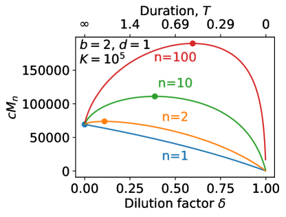
Figure 13: Expected number of mutations for different bottleneck sizes. The initial number of cells is $c=K\delta$. For a single cycle ($n=1$), smaller bottlenecks always yield more mutations. However, if more than one cycle is performed ($n\geq 2$), there is a non-zero optimal bottleneck size that maximises the expected number of mutations found in the population.

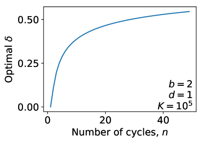
Figure 14: Mutation-optimising bottleneck size as a function of the number of cycles. The initial number of cells is $c=K\delta$. The bottleneck size that optimises the expected number of mutations is increasing with the number of cycles performed.

Proposition 7 shows that the number of mutation accumulated in a lineage is proportional to the mutation rate $\theta$. Moreover, since this number correspond to a single lineage, it must be multiplied by the number of initial lineages to obtain the total expected neutral diversity in a serial transfer protocol. In other words, doubling the mutation rate or doubling the initial number of cells doubles the expected number of mutations per droplet.

The expected number of mutations $M_{n}$ is also proportional to the expected coalescent tree length of a single extant lineage $L_{n}$ (weighted by the proportion of lineages that actually survive $s_{n}$). This expected coalescent length is parametrised by the birth and death rates of the particles, but also the duration of the growth phase $T$.

Figure 12 shows that the expected number of mutations increases indefinitely with the number of cycles. However, the rate of increase is tied to the dilution bottleneck and tends to slow down when the number of cycles increase. Note that for a small number of cycles, the expected number of mutations increases with a higher dilution: one cycle with a dilution by two yields less diversity than one cycle with a dilution by one hundred. However, if ten cycles are performed, a dilution by two yields more diversity. This illustrates a trade-off between a harsh bottleneck, that allows long cycles and thus potentially many mutations but leads to loss of most extant mutations (due to founder effects) and a softer bottleneck that allows for fewer mutations to accumulate during each cycle, but compounds more because fewer mutations are lost.

Figure 13 clarifies the link between the expected number of mutations and the dilution bottleneck. Note that smaller bottleneck sizes are compensated by longer cycles because the experiment is supposed to be performed in optimal conditions ($\delta=e^{-rT}$). If there is only one cycle ($n=1$), the maximal expected number of mutations is reached when the dilution bottleneck is vanishingly small ($\delta\to 0$) and the cycle length adequately long ($T\to\infty$). However, if there is more than one cycle ($n>1$) the expected number of mutations reaches a maximum value between $\delta=0$ and $\delta=1$. This maximum-diversity dilution bottleneck value increases with the number of cycles (Figure 14). Thus, the dilution bottleneck should be adjusted to the expected duration of the experiment in terms of cycle number to maximize accumulation of neutral mutations.

Overall, the expected number of neutral mutations accumulated by the population increases through time and can be optimised by appropriately choosing a bottleneck size that optimises the trade-off between accumulating new mutations and not losing old ones.

Note that $L_{n}$ behaves like $Tn\ln(n)$ (Lambert, (2009), Theorem 2.4), thus the expected neutral diversity after $n$ cycles is equivalent to $\theta s_{n}Tn\ln(n)$.

Thanks to (5), and because $\delta=\delta^{\star}=e^{-rT}$, we get:

$$M_{n}\sim_{n\to+\infty}\frac{\theta Tr}{b(1-e^{-rT})}\ln(n).$$

The mere number of mutations contains little information about the diversity within a droplet. Indeed, some of those mutations could be born by a single individual, while others might be shared by the whole population. The next section addresses this problem by exploring the mutation frequency spectrum.

3.5 Mutation Frequency spectrum

A more precise assessment of the neutral diversity structure involves distinguishing between rare mutations (that are carried by few individuals) and frequent mutations (that are widespread within the population). The mutation frequency spectrum presents the proportion of mutations that are carried by a given number of individuals. The expected mutation frequency spectrum of a coalescent point process can be deduced from the law of node depths $H$ ((Lambert,, 2009), Theorem 2.2). Indeed, the number of mutations carried by $i$ individuals is proportional to the length of the coalescent tree subtending $i$ leaves (Figure 15). As a result:

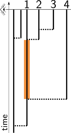
Figure 15: Finding the mutation frequency spectrum. Mutation shared by 3 individuals are the ones that arose within the orange region only. This region is delimited by $\max(H_{i+1},H_{i+2})<t<H_{i+3}$.

Proposition 8 (Mutation frequency spectrum)

Consider the Coalescent Point Process $\mathcal{T}_{n}$, with overlaying mutations following a Poisson point process with intensity $\theta$.

Let $M^{f}_{n}$ be the expected number of mutations fixed in the population, that is mutations shared by all individuals. Then:

$$M^{f}_{n}=\theta s_{n}\int_{0}^{nT}\frac{F(s)}{F(nT)}-\frac{F(nT)}{F(s)}ds$$ (11)

Let $a_{u}$ be the expected frequency of mutations that are shared by $u>0$ individuals in the limit of large sample of the population.

$$a_{u}=\theta\int_{0}^{nT}\left(1-\frac{\frac{1}{F(x)}-\frac{1}{F(nT)}}{1-\frac{1}{F(nT)}}\right)^{u-1}\left(\frac{\frac{1}{F(x)}-\frac{1}{F(nT)}}{1-\frac{1}{F(nT)}}\right)^{2}dx$$ (12)

(Proof page 7.)

As is expected for neutral diversity, Proposition 8 shows that the mutation frequency spectrum is proportional to the mutation rate $\theta$ meaning that an increasing proportion of individuals carry mutations if the rate increases, but that does not change the relative frequency of the size of groups carrying a given mutation.

Figure 16 shows the mutation frequency spectra for one and for a hundred cycles, and for three different dilution rates. Note that for a single cycle, harsher bottlenecks (i.e., smaller $\delta$, and correspondingly longer cycle duration $T$) increase the tail of the distribution (there are more mutations that are shared by many individuals). This effect of $\delta$ and $T$ is not as simple when considering several cycles. For $n=100$, the distribution is more heavy-tailed when the bottlenecks are soft ($\delta=0.5$) than when they are harsh ($\delta=0.001$).

Figure 17 shows the power law tail of mutation frequency spectra.

When the coalescent tree is a Kingman coalescent, corresponding to a long-lived population with approximately constant size, the mutation frequency spectrum has power law with exponent $-1$ (harmonic spectrum, Ewens’ sampling formula, (Ewens,, 1972)). In our setting, this happens when $\delta$ is close to 1 (constant population size) and $nT$ is large (long-lived population). For a fixed growth rate $r$, because $\delta e^{rT}=1$, this means that ($1-\delta$ is small but) $n(1-\delta)$ is large, as in the yellow region of the heat map of Figure 17.

When the coalescent tree is a Yule tree, corresponding to full, unbounded growth, the mutation frequency spectrum has power law with exponent $-2$ (Lambert,, 2009; Dinh et al.,, 2020). This is what happens for small $\delta$, regardless of $n$ as in the turquoise region of Figure 17. Indeed, when $\delta$ is small, $T$ is large (for fixed $r$), so that all derived mutations occurred since the last bottleneck.

A third case stands out in our setting when $n$ is not too large and $\delta$ sufficiently close to 1 that very few births/coalescences occur over the time interval of length $nT$, which happens when $n(1-\delta)=O(1)$. In this case, conditioning the CPP to have coalescences smaller than $nT$ (an event of vanishing probability) yields a CPP with uniform node depths, which gives rise to a power law mutation frequency spectrum with exponent $-3$, as in the deep blue region of Figure 17.

The information entropy of the mutation frequency spectrum can be used to systematically explore the effect of $\delta$ on the shape of the distribution. Figure 18 shows that if more than one cycle is performed, there is a value of $\delta$ that is expected to optimise the information entropy of the mutation frequency spectrum. This value is different from the value that optimises the number of mutations (Figure 13). Thus, there is a trade-off between accumulating many mutations, and having a diverse mutation frequency spectrum. The decision to fix $\delta$ in order to optimise one or the other depends on the goal of the experiment.

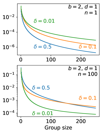
Figure 16: Mutation frequency spectrum. Give the frequency of mutations carried by a given number of individuals in a large sample of the population. Top: After $n=1$ cycle. Bottom: After $n=100$ cycles.

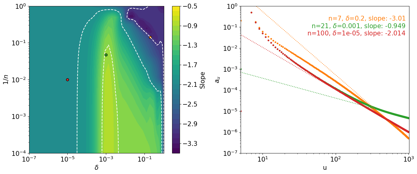
Figure 17: Mutation frequency spectrum power law tail. Left: Slope of the regression $\alpha$ such that $log(a_{u})=\alpha log(u)+b$, for $u>500$. For a branching process without bottleneck the expected value is $-2$, it is $-1$ for a Moran process and $-3$ for a CPP with uniform node depths. White dashed lines are isolines $-1$, $-2$, $-3$. Right: Three illustrative mutation frequency spectra with associated regression lines. The location of the three spectra in the parameter space is represented by color-matching dots on the left heatmap.

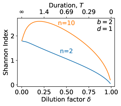
Figure 18: Shannon Entropy of the mutation frequency spectrum. Defined as $S=-\sum_{i}a_{i}\log(a_{i})$

To sum up, higher dilution rate or longer duration of collective growth cycles result in longer trees and increased diversity, even though the population may risk going extinct. Extinction of the population marks the “death” of the culture, and it is the eventual fate of a serial transfer experiment in the limit of many cycles. In a nested population design, the cultures can also “reproduce” and replace the extinct ones. This has far-reaching consequences on the genealogy of the particles, as shown in the next section.

4 Diversity in Dividing Droplets

Nested populations’ design differ from simple serial transfer in parallel cultures by the opportunity for the cultures (droplets, tubes or other compartments) to be subject to birth and death themselves. At each cycle, some cultures may be removed from the experiment, while others can be duplicated, usually by dispatching samples of the original collective in several new fresh medium compartments (rather than one in regular parallel serial transfer experiments).

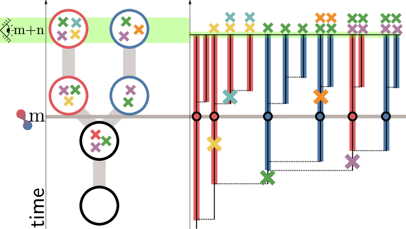
Figure 19: Collective and Particle nested coalescent trees. Left: coalescent tree of droplets. Right: coalescent tree of particles. An ancestral droplet lineage (black) is diluted into two offspring droplets (red, blue). At the time when the droplets are split (cycle $m$), the particle lineages within the ancestral droplets are assigned a colour (red or blue) that indicates the daughter droplet to which they are sent. Mutations appear along the genealogy of particles (crosses). Some mutations appear before the split (yellow, green, purple) and are found in both droplets (green, purple) if they are sampled by both droplet lineages, or within a single droplet (yellow) if they are segregated by the dilution. Other mutations appear after the split (light blue, orange) and are only found in one of the droplet lineages.

This section focuses on the consequences of imposing a collective-level birth-death process on the neutral diversity. To this end, consider the simple scenario (depicted in Figure 19) of a pair of droplets that share a common “droplet ancestor” several cycles in the past. The two droplets differ by the initial sampling performed in their common ancestor, and also by all new mutations accumulated since they became isolated.

In the following, the particles follow a super-critical linear birth-death process with parameters $b-d=r>0$. The parameters of the population structure are supposed to be optimal in the sense of Section 2.1: each cycle has a duration $T^{*}=-r^{-1}\ln{(cK^{-1}})$ and each lineage has an independent probability of being sampled at a bottleneck of $\delta^{*}=e^{-rT^{*}}$. Consider that the droplet split happens at cycle $m$ and the observation occurs at cycle $m+n$.

4.1 Survival probability

First, let us consider the probability that a lineage spawned by a single cell $n$ cycles in the past is not extinct within both droplets. The key to establish this probability is to recognise that the lineage undergoes a bottleneck with survival probability $\delta$ at each cycle, except the cycle of the droplet split where each particle has a probability $2\delta$ to survive. Indeed, two inoculation volumes are concurrently sampled from the ancestral droplet and dispatched into two offspring (Figure 20). Thus:

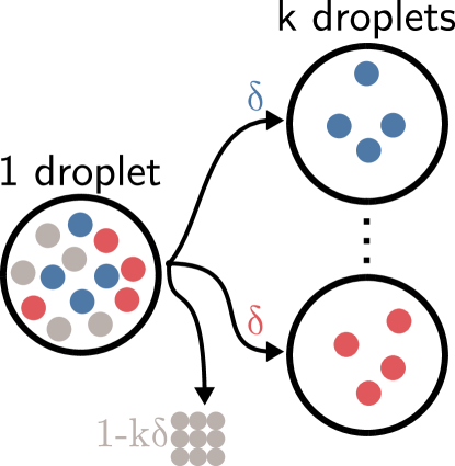
Figure 20: Droplet Splitting Process. When a droplet is split into $k$ droplets, individual particles are independently selected to be transferred to the next cycle (with probability $\delta$ for each new droplet) or sent to the waste (with probability $1-k\delta$).

Proposition 9 (Survival probability - Split droplet)

Cells within droplets in serial transfers are modelled by a linear birth-death process with constant parameters $b$ and $d$, that is subject to periodic bottlenecks every duration $T$. Additionally, consider that at the $m$th cycle, the dilution procedure is repeated to obtain $k$ new droplets.

Let $s_{k,m,n}$ be the probability that a lineage spawned by a single cell is not extinct at the end of the $(n+m)$th cycle.

$$s_{k,m,n}=1-h_{Q_{k,m,n}}(0),$$

Where $h_{A}$ the linear fractional function with coefficient $A$ defined in Equation 1. The matrix $Q_{k,m,n}$ is the product:

$$Q_{k,m,n}=Q_{1}^{m-1}Q_{k}Q_{1}^{n-1}R$$

with,

$$\forall k\in\mathbb{N}^{*},\;Q_{k}=\begin{bmatrix}k\delta(p-q)&p-k\delta(p-q)\\ k\delta(p-1)&p-k\delta(p-1)\end{bmatrix};\;\;\;R=\begin{bmatrix}\delta(p-q)&q\\ \delta(p-1)&1\end{bmatrix}$$

Where $\delta$ is the survival probability of a particle at serial transfer, $q$ is the extinction probability of a lineage during a cycle, and $p$ the geometric parameter of the size of a non-extinct lineage as defined in Proposition 1.

(Proof page 8.)

Proposition 9 is similar in its conclusion to Proposition 1, that treated case of a simple serial transfer. However, the expression is considerably less easy to handle, as the iteration does not simplify into a single matrix power.

4.2 Total diversity

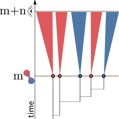
Figure 21: Finding the total diversity at cycle $n+m$ of droplets split at cycle $m$. All the lineages (triangles) spawned from the particles dispatched in one of the $k=2$ droplets (here red and blue) have the same expected length $L_{n}$. The bottom part (or stump) of the tree (black) result from the sampling of a CPP stopped in $mT$, with probability $\pi_{k,m,n}$, the probability that an extant lineage at cycle $m$ will be sampled in one of the two droplets, and survive until cycle $n+m$.

As seen in Proposition 7, quantifying the total neutral diversity in an infinitely-many sites model is a matter of finding the total length of the coalescent tree (or forest) of the population. Note that the full coalescent tree in Figure 21 can be decomposed into a stump, before the splitting of droplets, and a corolla: another set of CPP (the corolla) sampled in one or the other droplet lineage. As a result:

Proposition 10 (Total Diversity - Split droplet)

Let $M_{k,m,n}$ be the expected number of mutations accumulated in a lineage at cycle $n+m$ after the splitting of the initial droplet at cycle $m$ into $k=1,2\ldots\left\lfloor\frac{1}{\delta}\right\rfloor$ droplets. Then:

$$M_{k,m,n}= \theta L_{k,m,n}$$

$$= \theta s_{m}F^{\dagger}(mT)\left[\int_{0}^{mT}\frac{1}{F^{\dagger}(s)}ds+\int_{0}^{nT}\frac{F(nT)}{F(s)}ds\right],$$

where $L_{k,m,n}$ is the expected length of the coalescent tree of the population, $F$ is the inverse tail distribution of the CPP with periodic bottlenecks, and $F^{\dagger}:=1-k\delta s_{n}+k\delta s_{n}F$, is the inverse tail distribution of the same CPP submitted to sampling with probability $k\delta s_{n}$ at the present.

(Proof page 9.)

4.3 Private Diversity

In order to assess the divergence between split droplets, one can compute the expected number of private mutations, i.e., mutations that are only found in a single of the $k$ split droplets. This number is the sum of all mutations that occur in the droplets after the splitting time $mT$ (i.e., mutations in the corolla), plus all the mutations that occur before the splitting time but in a lineage that only segregates in a single droplet (i.e., mutations in the stump). Since all the droplet are interchangeable, this value is identical for the $k$ droplets. Overall, this number is proportional to the red (or blue) part of the CPP in figure 19.

Proposition 11 (Private Mutations - Split Droplet)

Let a single droplet be split into $k=1\ldots\left\lfloor\frac{1}{\delta}\right\rfloor$ at cycle $m$. Let $M^{\prime}_{k,m,n}$ be the expected number of mutations that are private to any of the $k$ droplets when observed at cycle $n+m$.

$$M^{\prime}_{k,m,n} =\underbrace{\mathcal{S}_{k,m,n}}_{\text{stump}}+\underbrace{\mathcal{C}_{k,m,n}}_{\text{corolla}}$$

$$=\theta s_{m}F^{\dagger}(mT)\left[\int_{0}^{mT}\frac{kds}{F^{\dagger}(s)(1+(k-1)F^{\dagger}(s))}+\int_{0}^{nT}\frac{F(nT)}{F(s)}ds\right],$$

where $F$ is the inverse tail distribution of the CPP with periodic bottlenecks, and $F^{\dagger}$ is the inverse tail distribution of the same CPP submitted to sampling with probability $k\delta s_{n}$ at the present.

(Proof page 10.)

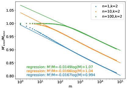
Figure 22: Expected Proportion of private mutations in split droplets. Droplets are grown for $m$ cycles, then split into $k=2$ new droplets and grown for $n$ new cycles. $b=1,d=0,\delta=e^{-rT}$

Figure 22 shows the expected proportion of private mutations $M^{\prime}_{k,m,n}/M_{k,m,n}$ in split droplets as a function of $m$, the number of cycles before splitting. If $m$ is low, there are no shared mutations among droplets and the ratio is close to $1$. If more cycles occur before the split, the proportion of private mutations decreases, tending at a logarithmic speed to 0. Now, the main purpose of droplet splitting is to select and duplicate a phenotype of interest. The last section explores, in the context of artificial selection, the advantage offered by a droplet-splitting process over the simple screening of parallel cultures in serial transfer.

5 Artificial selection of droplets

A practical application of a device that would allow the manipulation of small cultures of microbial organisms would be the artificial selection of phenotypes of interest. Suppose that a given phenotype of interest is reached after the accumulation of $\Theta$ mutations, and that it is possible to detect the number of mutations fixed so far, by sequencing or direct observation of the cultures.

To formalise, let $D\in\mathbb{N}^{*}$ be the number of collectives. Each collective $i$ is assigned a number $e_{i}=1,2,\ldots,\Theta$, corresponding to the number of fixed mutations. Suppose that the time for a collective to switch from $e_{i}=j$ to $e_{i}=j+1$ is exponentially distributed with parameter $\alpha=\frac{\rho}{ND}$, where $\rho$ is the mutation rate (that could be deduced from Proposition 8), scaled by the number of droplets $D$ and the number of cycles $N$. We assume that the $D$ collectives are in state $0$ at time $0$. The only possible transition is to accumulate a new mutation, no reversion is possible, as illustrated in Figure 23.

Figure 23: Phenotypes. There are $\Theta+1$ possible phenotypes. A $j\text{-collective}$ switches to the next phenotype $j+1$ at rate $\alpha$.

In order to assess the advantage of droplet splitting, consider two scenarios, illustrated in Figure 24:

1. Without collective selection $D$ collective lineages are started in state $0$ at $t=0$ and undergo serial transfer independently of each other.

2. With collective selection $D$ collective lineages are started in state $0$ at $t=0$, once a mutant is detected in a lineage, all the other collectives are killed and this lineage is split in $D$ new lineages.

Let $\Gamma$ (respectively $\Gamma^{*}$) be the random variable encoding the first time for a lineage to get to the state $\Theta\in\mathbb{N}$ in the scenario without collective selection (respectively with collective selection). To compare them, consider their respective cumulative distribution functions:

Figure 24: Propagation of mutations. Without collective selection, all the lineages accumulate mutations independently. With collective selection, once a mutation fixation is first detected, the droplet is split into $D$ lineages.

Proposition 12 (Cumulative distribution functions)

The cumulative distribution function of $\Gamma^{*}$ is:

$$\mathbb{P}(\Gamma^{*}\leq x)=1-e^{-x\rho}\left(\sum^{\Theta-1}_{u=0}\frac{(\rho x)^{u}}{u!}\right)$$ (13)

The cumulative distribution function of $\Gamma$ is:

$$\mathbb{P}(\Gamma\leq x)=1-e^{-\rho x}\left(\sum^{\Theta-1}_{u=0}\frac{(\rho x)^{u}}{D^{u}u!}\right)^{D}$$ (14)

When the number of mutational steps tends to infinity, the two cumulative distribution function are equivalent. However, for any finite number of mutational steps $\Theta$, the selective regime is faster than the serial transfer regime.

(Proof page 11.)

Proposition 12 shows that collective level selection, i.e., the process of splitting a droplet in which an intermediate mutation was fixed, leads to reducing the time to reach the $\Theta\text{-th}$ mutation. Figure 25 shows the shape of the cumulative probability function for both regimes, illustrating this advantage. This constitutes a simple use-case for a device that allows the automated high-throughput manipulation of numerous cultures, such as the digital millifluidic analysers (Baraban et al.,, 2011; Boitard et al.,, 2015; Cottinet et al.,, 2016).

Note that this result is obtained by assuming that the detection of mutation is cost-less and error-free. A more advanced model of this system should tackle the problem of imperfect detection.

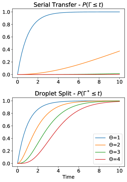
Figure 25: Cumulative probability distribution of the time to accumulate $\Theta$ mutations. With droplet splitting, accumulation of mutation is faster. $D=100$.

6 Discussion

This manuscript has laid the foundation for a theoretical understanding of the evolution of neutral diversity in massively parallel microbial evolution experiments. It was heavily inspired by ongoing engineering efforts to bring experimental evolution to digital millifluidics (Cottinet,, 2013; Boitard et al.,, 2015; Dupin,, 2018; Doulcier,, 2019).

In experimental microbiology, one desirable feature can be to maximise the number of mutations accumulated within the cultures, for instance in order to screen phenotypes of interest. The result presented above showed that, in an optimal growth setting, where cells are growing with a constant birth and death rate, without density-dependence or competition, the population should be submitted to cycles whose duration is tailored to compensate the bottleneck imposed at each serial transfer. The choice of the bottleneck should be made according to the expected duration of the experiment: in order to optimise the expected number of mutations, small bottlenecks (killing most of the lineages) should be used when the number of cycles is small, while larger bottlenecks (lower dilution rate) should be used for long term experiments. Additionally, the expected number of mutations increases linearly with increasing droplet volume and with increasing number of droplets which is a matter of technological progress as automation and larger droplet sizes are under consideration (Dupin,, 2018; Postek et al.,, 2022). The mutation rate also increases linearly the number of expected mutations and can be manipulated by choosing mutator lineages or adding mutating chemicals to the culture broth. However, the potentially deleterious effects of this method might prevent using it in practical cases.

In long-term evolution experiments (Kawecki et al.,, 2012; Van den Bergh et al.,, 2018), serial transfer is imposed by the need to replenish nutrients available to the cells. It is possible to build devices ensuring that a continuous flow of nutrient washes over the culture (for large volumes, see chemostats, or morbidostats (Toprak et al.,, 2013), in microfluidics, see mother machines (Potvin-Trottier et al.,, 2018). However, these methods are usually more prone to contamination. In contrast, periodically diluting the culture in fresh medium is simple and robust.

The nested population design differs from traditional serial transfer of parallel cultures because it allows a collective birth-death process at the level of collectives. Serial transfer is pervasive in experimental evolution (Kawecki et al.,, 2012), and has received extensive theoretical treatment. So far we have only focused on neutral diversity. The effect of beneficial mutations has been studied in serial transfer settings. In particular, the probability of losing a beneficial mutation because of repeated bottlenecks (Wahl and Krakauer,, 2000; Wahl et al.,, 2002; Wahl and Gerrish,, 2001; Wahl and Zhu,, 2015), and the effect of bottlenecks on the evolutionary path when multiple beneficial mutations exist (Gamblin et al.,, 2023). This work should be extended to the nested population design in the future.

In practice, the collective birth-death process can come from the fact that some cultures are effectively empty because of high dilutions in the previous cycle, and may be replaced in the next cycle by cells from a non-empty culture. The use of collective birth-death processes can also be a consequence of the experimental protocol. Milli and microfluidics compartments are usually produced in large numbers, while measurements are performed on all compartments, the retrieval of all the compartment’s content might not be practically possible or even desirable when they are too numerous. Finally, the collective birth-death process may stem from an active effort of the operator to select some populations based on some measurable characteristics.

The use of a non-saturating population dynamics in this manuscript is a simplification that should be carefully taken into account when transposing the results of this work to the design of experiments. Nonetheless, if the cycle duration is short enough so that the population is stopped during exponential phase, the heuristics developed in this manuscript should hold. There are however two phenomena that were not modelled here and that will probably muddy the neutral pattern that was described. First, the absence of mutations affecting birth and death rates. If most point-mutations can be safely considered neutral, some rare mutations can affect the ability to reproduce of the cells. If the mutations are beneficial, they will increase in proportion within the population, and will change the relative frequency of all neutral mutations, by favouring the ones carried by the same strand of DNA. This is a well documented phenomenon known as hitch-hiking (Fay and Wu,, 2000). Second, horizontal gene transfer might allow the uncoupling of the mutation transmission from the genealogy (Dutta and Pan,, 2002), muddying the pattern even further.

The nested population design also differs from trait groups (Wilson,, 1975) or transient compartments (Blokhuis et al.,, 2018) population structure because migration between compartments is prevented. As a consequence, it is possible to construct a non-ambiguous genealogy of the cultures. In practice, serial transfer design offers a natural way to implement the birth-death process, by diluting some cultures into several new compartments (the droplet splitting) and discarding others.

Finally, this manuscript touches briefly the problem of artificial selection using a nested population design. This was done by considering the accumulation of neutral mutations. A more complete model of artificial selection would, however, take into account interactions between individuals, and potentially the selection of whole communities. Community-level selection has been the subject of both experimental (Swenson et al.,, 2000; Panke-Buisse et al.,, 2015) and theoretical inquiries (Arias-Sánchez et al.,, 2019; Xie et al.,, 2019; Doulcier et al.,, 2020).

Overall, the results presented in this manuscript should be considered as a way to build intuition about the experimental system, while providing a null-model for diversity that could be compared to the actual patterns. Inevitable differences have to appear, but the point of comparison that is offered by neutral evolution will allow a better description of the observed diversity. Focusing on the part of the patterns that differ from this naive theoretical prediction will surely be fruitful: it shows that other mechanisms than drift must be invoked.

Reference

Table 2: Global Symbols reference

Symbol	Name	Reference
$D$	Collective Population size
$T$	Cycle duration
$n$	Number of Cycles
$K$	Collective Carrying capacity
$c$	Initial number of particles
$b,d,r$	Particle birth rate, death rate and Malthusian parameter ($r:=b-d$)
$\delta$	Particle Survival probability (at a bottleneck)
$\theta$	Particle Mutation rate
$s_{n}$	Probability that a lineage spawned by a single particle is not extinct at the end of the $n$th cycle. (At time $nT^{-}$, just before the $n$th dilution). $s_{n}=1-h_{Q^{n-1}R}(0)$	Proposition 1
$s_{\infty}$	Limit probability that a lineage spawned by a single particle is not extinct after a large number of cycles. $s_{\infty}=\lim_{n\to\infty}s_{n}$.	Proposition 2
$T^{*}$	Maximal cycle duration before reaching saturation. $T^{*}=r^{-1}ln(cK^{-1})$	Proposition 3
$\delta^{*}$	Optimal dilution rate $\delta^{*}=e^{-rT}$	Proposition 4
$s^{*}_{n}$	Survival probability of a lineage spawned by a single cell before the $n$th dilution in the optimal regime in which $\delta=e^{-rT}$.	Proposition 5
$\tilde{F}$	Inverse tail distribution of the CPP without bottlenecks	Proposition 6
$F$	Inverse tail distribution of the CPP with bottlenecks. $F(t)=[\mathbb{P}(H>t)]^{-1}$	Equation 6 and Proposition 6
$\tau_{n}$	Coalescent tree of an extant lineage at the end of the $n$th cycle. It is a Coalescent Point Process with inverse tail distribution $F$ stopped at the first branch length larger than $nT$.	Proposition 7
$N(\tau_{n})$	number of leaves of the coalescent tree $\tau_{n}$. Geometric random variable with expected value $F(nT)$.	Eq. 15 and 16.
$L_{n}$	Expected length of the coalescent tree $\tau_{n}$. $L_{n}=F(nT)\int_{0}^{nT^{-}}F(x)^{-1}dx$	Proposition 7
$M_{n}$	Expected number of mutations in a lineage after $n$ cycles. $M_{n}=\theta s_{n}L_{n}$	Proposition 7
$M^{f}_{n}$	Expected number of fixed mutations in a lineage after $n$ cycles.	Proposition 8
$M^{s}_{n}$	Expected number of segregating mutations in a lineage after $n$ cycles. $M^{s}_{n}=M_{n}-M^{f}_{n}$	Proposition 8
$a_{u}$	Expected frequency of mutations shared by $u>0$ individuals after $n$ cycles.	Proposition 8

Table 3: Global Symbols reference (cont)

Symbol	Name	Reference
$s_{k,m,n}$	Survival probability at the end of the $(m+n)$th cycle of a lineage spawned by a single cell in a single droplet at the first cycle, that is was split into $k$ droplets at cycle $m$.	Proposition 9
$\tau_{k,m,n}$	Coalescent tree at the end of the $(m+n)$th cycle of a lineage spawned by a single cell in a single droplet at the first cycle, that is was split into $k$ droplets at cycle $m$.	Proposition 10
$\pi_{k,n}$	Probability that a lineage extant at the end of cycle $m$ just before the droplet is split into $k$ droplets will be extant at cycle $m+n$. $\pi_{k,n}=k\delta s_{n}$.
$F^{\dagger}$	Inverse tail distribution of the stump tree. $F^{\dagger}(t):=F_{\pi_{k,n}}(t)=1-\pi_{k,n}+\pi_{k,n}F(t),t\in[0,mT]$
$L_{k,m,n}$	Expected length of the Coalescent tree $\tau_{k,m,n}$	Proposition 10
$M_{k,m,n}$	Expected number of mutations accumulated at the end of the $(m+n)$th cycle of a lineage spawned by a single cell in a single droplet at the first cycle, that is was split into $k$ droplets at cycle $m$. $M=\theta s_{k,m,n}L_{k,m,n}$
$M^{\prime}_{k,m,n}$	Expected number of mutations that are only found in a single droplet at the end of the $(m+n)$th cycle of a lineage spawned by a single cell in a single droplet at the first cycle, that is was split into $k$ droplets at cycle $m$.	Proposition 11

Table 4: Global Symbols reference (cont.)

Symbol	Name	Reference
$\alpha$	Rate at which a lineage accumulate mutations $\alpha=\frac{\rho}{ND}$	Proposition 12
$\Theta$	Number of mutations to accumulate	Proposition 12
$\Gamma$	First time a lineage has accumulated $\Theta$ mutations without collective selection	Proposition 12
$\Gamma^{*}$	First time a lineage has accumulated $\Theta$ mutations with collective selection	Proposition 12

Appendix A Reproducing the figures

The code used to generate all the figures in the manuscript uses python 3.11, matpolotlib 3.6.3, numpy 1.24.2 and scipy 1.24.2. It is available on the Zenodo repository under the DOI 10.5281/zenodo.8087961.

Appendix B Proofs

In this section we give the mathematical proofs for the results used in the main text.

Parameters range

Proof 1 (Proposition 1 - Survival Probability)

Let $s_{n}$ be the survival probability at $t=nT$ of a lineage started from a single cell at $t=0$.

First cycle

Consider one cell at time $t=0$. This cell follows a Linear Markov Branching Process $(Z_{t})_{t\in[0,T)}$ with constant rates $b,d$ until the dilution time $T$. The branching process goes extinct ($Z_{t}=0$) with probability $q(b,d,t):=\mathbb{P}(Z_{t}=0)$, and conditional on non-extinction $Z_{t}$ follows a geometric distribution with parameter $p(b,d,t)$, that is, $\mathbb{P}(Z_{t}=k|Z_{t}\neq 0)=p(1-p)^{k-1}$.

		$p(b,d,t)$	$q(b,d,t)$
Subcritical particles	$r<0$	$\frac{d-b}{d-be^{rt}}$	$\frac{d(1-e^{rt})}{d-be^{rt}}$
Critical particles	$r=0$	$\frac{1}{1+bt}$	$\frac{bt}{1+bt}$
Supercritical particles	$r>0$	$\frac{(b-d)e^{-rt}}{b-de^{-rt}}$	$\frac{d(1-e^{-rt})}{b-de^{-rt}}$

The probability generating function of $Z_{T}$ is:

$$f_{Z_{T}}(s) =\sum_{k\geq 0}\mathbb{P}(Z_{T}=k)s^{k} \text{Definition of }f$$

$$=\mathbb{P}(Z_{T}=0)s^{0}+\sum_{k\geq 1}\mathbb{P}(Z_{T}=k)s^{k}$$

$$=\mathbb{P}(Z_{T}=0)s^{0}+\sum_{k\geq 1}\mathbb{P}(Z_{T}\neq 0)P(Z_{T}=k|Z_{T}\neq 0)s^{k}$$

$$=q+\sum_{k\geq 1}(1-q)p(1-p)^{k-1}s^{k} \text{Definition of }p,q$$

$$=q+ps(1-q)\sum_{k\geq 0}((1-p)s)^{k}$$

$$=q+\frac{ps(1-q)}{1-(1-p)s} \text{Geometric series, }(1-p)s<1$$

$$=\frac{s(p-q)+q}{s(p-1)+1}$$

Note that, as expected, $f_{Z_{T}}(1)=1$ and $f_{Z_{T}}(0)=P(Z_{T}=0)=q$.

Note that $f_{Z_{T}}$ is linear fractional, a property that will be useful later when composing generating functions. We associate any linear-fractional function $h_{M}$ with a coefficient matrix $M$ as follows:

$$M=\begin{bmatrix}a&b\\ c&d\end{bmatrix}\Leftrightarrow h_{M}(s)=\frac{as+b}{cs+d}$$

We define:

$$Q_{0}:=\begin{bmatrix}p-q&q\\ p-1&1\end{bmatrix},$$

such that $f_{Z_{T}}=h_{Q_{0}}$.

Second cycle

Consider a cell at the end of the first cycle, just before the first dilution. It Let $B$ be the number of descendants of this cell at the end of the second cycle. There are two possibilities to consider.

First, with probability $(1-\delta)$, the cell is discarded during the dilution at the beginning of the second cycle and $B=0$.

Second, with probability $\delta$, the cell is not discarded, and thus sees its descent grow until the end of the cycle following the same law as in the first circle, namely the law of $Z_{T}$, so that $f_{B}=1-\delta+\delta h_{Q_{0}}=h_{Q}$, where:

$$Q:=\begin{bmatrix}p-1+\delta(1-q)&1-\delta(1-q)\\ p-1&1\end{bmatrix}.$$

Subsequent cycles

Let $X_{n}$ be the number of descendants of an ancestral cell at the end of the $n$th cycle. Let $(B_{n,i})_{n>0,i>0}$ be a collection of identical and independent random variables following the same law as $B$. Then $X_{1}$ follows the same law as $Z_{t}$ and the following recursion holds:

$$X_{n}=\sum_{i=1}^{X_{n-1}}B_{n,i}$$

Thus, the generating function of $X_{n}$ is given by the composition of the generating functions of $X_{1}\ldots X_{n}$.

The composition of two linear fractional functions with associated matrices $M_{1}$ and $M_{2}$ is a linear fractional function with associated coefficient matrix $M_{1}M_{2}$. By simple induction, for n $\in\mathbb{N}$ the iterated composition is obtained by computing the matrix power: $h^{n}_{M}=h_{M^{n}}$.

It results that:

$$f_{X_{n}}=h_{Q_{0}Q^{n-1}}$$

This leads to the survival probability of the lineage spawned by an ancestral cell, at the end of cycle $n$:

$$s_{n}=1-f_{X_{n}}(0)=1-h_{Q_{0}Q^{n-1}}(0)$$

Proof 2 (Proposition 2 - Long Term Survival Probability)

Let us look for the fixed points of $f_{B}$:

$$f_{B}(s)=s \Leftrightarrow(p-1+\delta(1-q))s+1-\delta(1-q)=s((p-1)s+1)$$

$$\Leftrightarrow(s-1)((p-1)s+\delta(1-q)-1)=0$$

$$\Leftrightarrow s=\frac{\delta(1-q)-1}{p-1} \text{or }s=1$$

$f_{B}(s)-s$ is a second order polynomial for $s$ meaning that $f_{B}$ has at most two fixed points. One of them is 1, in accordance with the definition of characteristic functions. The other is $s^{*}$, with

$$s^{*}<1\Leftrightarrow p<\delta(1-q)$$

Since $f_{B}$ is continuous, $f_{B}(s)\geq s$ for all $s\in[0,\min(s^{*},1)]$ and $\min(s^{*},1)$ is a fixed point of $f_{B}$, the sequence $u_{n}=f_{B}(u_{n-1})$ with $u_{0}=h_{Q_{0}}(0)\in[0,1]$ converges to $\min(s^{*},1)$, that is, to $1$ if $p>\delta(1-q)$ and to $s^{*}$ otherwise.

• In Subcritical regime, $p<\delta(1-q)\Leftrightarrow e^{-rT}<\delta$, is always false since $e^{-rT}>1$ and $\delta\leq 1$.

• In Critical regime, $p<\delta(1-q)\Leftrightarrow\frac{1}{1+bT}<\delta\left(1-\frac{bT}{1+bT}\right)=\delta\frac{1}{1+bT}$, is always false since $\delta\leq 1$.

• In Supercritical regime, $p<\delta(1-q)\Leftrightarrow e^{-rT}>\delta$,

Thus, $s^{*}>1$ except if $b>d$ and $\delta<e^{-rT}$. In this case,

$$s_{\infty} =1-h_{Q_{0}}(s^{*})$$

$$=\frac{\delta(p-q)-p}{\delta(1-q)}$$

$$=\frac{r(\delta-e^{-rT})}{\delta b(1-e^{-rT})}$$

Proof 3 (Proposition 4 - Critical dilution)

We define $\delta^{*}$ as the dilution parameter preventing the number of cells to grow unbounded. More precisely, we want the expected number of cells to remain constant between two dilutions.

Recall that $B$ be the number of descendants of an initial cell after one cycle. The generating function of $B$ is $f_{B}$ as defined in proof 1. Note that $\mathbb{E}(B)=f_{B}^{\prime}(1)$.

When $\delta=\delta^{*}$, we expect the number of descendants after one cycle to be constant, thus $\mathbb{E}(B)=1$.

$$f_{B}^{\prime}(1) =\delta^{*}\frac{1-q}{p}=1$$

$$\delta^{*} =\frac{p}{1-q}$$

When the particles are supercritical, $0<d<b$:

$$\delta^{*} =\frac{(b-d)e^{-(b-d)T}}{b-de^{-(b-d)T}}\frac{b-de^{-(b-d)T}}{b-de^{-(b-d)T}-d(1-e^{-(b-d)T})}$$

$$=e^{-(b-d)T}$$

Proof 4 (Proposition 5 - Critical survival Probability)

Let $\delta=e^{-rT}$, $r=b-d$, $r>0$.

Then, the probability of extinction of the branching process is:

$$q=\frac{d(1-\delta)}{b-d\delta}$$

The parameter of the geometric distribution of the number of particles, conditional on non extinction, is:

$$p=\frac{r\delta}{b-d\delta}$$

Thus, it is possible to rewrite $Q_{0}$ and $Q$ like this:

$$Q_{0}=\frac{1}{b-\delta d}\begin{bmatrix}\delta b-d&d(1-\delta)\\ b(\delta-1)&b-\delta d\end{bmatrix}:=\frac{1}{b-\delta d}\overline{Q_{0}}$$

$$Q=\frac{1}{b-\delta d}\begin{bmatrix}2\delta b-\delta d-b&b(1-\delta)\\ b(\delta-1)&b-\delta d\end{bmatrix}:=\frac{1}{b-\delta d}\overline{Q}$$

By induction, we can show that:

$$s_{n}^{*}=1-h_{Q_{0}Q^{n-1}}(0)=\frac{(Q_{0}Q^{n-1})_{01}}{(Q_{0}Q^{n-1})_{11}}=\frac{\overline{Q_{0}Q^{n-1}}_{01}}{\overline{Q_{0}Q^{n-1}}_{11}}=\frac{b-d}{bn-\delta(b(n-1)+d)}=\frac{r}{bn(1-\delta)+\delta r}$$

Coalescent Point Processes

Proof 5 (Proposition 6 - Coalescent tree)

Consider the CPP of the population just before the $n$th cycle of dilution. The population experienced $n-1$ bottlenecks at times $t_{1}=(n-1)T,\ldots,t_{n-2}=2T,t_{n-1}=T$.

Let $\{H_{ij},(i,j)\in\mathbb{N}^{2}\}$ be a set of i.i.d. random variables following the same law as $H$, defined by its inverse tail distribution $F(t)=\frac{1}{\mathbb{P}(H>t)}$, where $F$ is the scale function of the CPP with bottlenecks.

Let $\tilde{F}$ be the scale function of the CPP without bottleneck. Using Proposition 7 in Lambert and Stadler, (2013) with $\epsilon_{i}=\delta$ and $s_{i}=iT$, $t=nT+s$, with $n=\left\lfloor\frac{t}{T}\right\rfloor\in\mathbb{N}$ and $s<T$, it is possible to write $F$ as:

$$F(t)=\delta^{n}\tilde{F}(nT+s)+(1-\delta)\sum_{j=0}^{n-1}\delta^{j}\tilde{F}(jT)$$

If the sampling at the last cycle is taken into account, the scale function becomes $\overline{F}$:

$$\overline{F}(t)=1-\delta+\delta F(t)$$

The expression of $\tilde{F}$ is known for the most common birth-death processes:

	Parameters	Scale function
Pure Birth	$0=d<b$	$\tilde{F}(t)=e^{bt}$
Non-critical	$0<d\neq b>0$	$\tilde{F}(t)=\frac{b}{r}(e^{rt}-1)+1$
Critical	$0<d=b$	$\tilde{F}(t)=bt+1$

Non-critical case $r:=b-d\neq 0,b>0,d>0$:

$$F(nT+s) =\delta^{n}\left[1-\frac{b}{r}+e^{r(nT+s)}\frac{b}{r}\right]+(1-\delta)\sum_{j=1}^{n}\delta^{j-1}\left[e^{rjT}\frac{b}{r}+1-\frac{b}{r}\right]$$

$$=\delta^{n}\left(1-\frac{b}{r}\right)+\frac{b}{r}e^{rs}(\delta e^{rT})^{n}+(1-\delta)\left[\left(1-\frac{b}{r}\right)\sum_{j=0}^{n-1}\delta^{j}+\frac{b}{r}e^{rT}\sum_{j=0}^{n-1}(\delta e^{rT})^{n}\right]$$

$$=\delta^{n}\left(1-\frac{b}{r}\right)+\frac{b}{r}e^{rs}(\delta e^{rT})^{n}+\left(1-\frac{b}{r}\right)(1-\delta^{n})+\frac{b(1-\delta)}{r}e^{rT}\sum_{j=0}^{n-1}(\delta e^{rT})^{j} \text{(Geometric series, }\delta\neq 1)$$

$$=1+\frac{b}{r}\left[e^{rs}(\delta e^{rT})^{n}-1+(1-\delta)e^{rT}\sum_{j=0}^{n-1}(\delta e^{rT})^{j}\right]$$

If $\delta\neq\delta^{*}$ then,

$$F(nT+s) =1+\frac{b}{r}\left[e^{rs}(\delta e^{rT})^{n}-1+(1-\delta)e^{rT}\frac{1-(\delta e^{rT})^{n}}{1-\delta e^{rT}}\right] \text{(Geometric series, }\delta^{*}e^{rT}\neq 1)$$

Otherwise, if $\delta=\delta^{*}=e^{-rT}$,

$$F(nT+s)=1+\frac{b}{r}\left(e^{rs}-1+n(e^{rT}-1)\right)$$

Pure-birth case $d=0$

$$F(nT+s) =\delta^{n}e^{b(nT+s)}+(1-\delta)\sum_{j=1}^{n}\delta^{j-1}e^{jbT}$$

$$=e^{bs}(\delta e^{bT})^{n}+(1-\delta)\sum_{j=0}^{n-1}\delta^{j}e^{(j+1)bT}$$

$$=e^{bs}(\delta e^{bT})^{n}+(1-\delta)e^{bT}\sum_{j=0}^{n-1}\left(\delta e^{bT}\right)^{j}$$

If $\delta\neq\delta^{*}=e^{-bT}$, then since $\delta e^{bT}\neq 1$, we can apply the geometric series expression:

$$F(nT+s)=e^{bs}(\delta e^{bT})^{n}+(1-\delta)e^{bT}\frac{1-\left(\delta e^{bT}\right)^{n}}{1-\delta e^{bT}}$$

Otherwise, $\delta e^{bT}=1$:

$$F(nT+s)=e^{bs}+n(e^{bT}-1)$$

Critical case $b=d\neq 0$

$$F(nT+s)= \delta^{n}(b(nT+s)+1)+(1-\delta)\sum_{j=1}^{n}\delta^{j-1}(bjT+1)$$

$$= \delta^{n}(b(nT+s)+1)+(1-\delta)\sum_{j=0}^{n-1}\delta^{j}(b(j+1)T+1)$$

$$= \delta^{n}(b(nT+s)+1)+(1-\delta)\left[(1+bT)\sum_{j=0}^{n-1}\delta^{j}+bT\sum_{j=0}^{n-1}j\delta^{j}\right]$$

$$= \delta^{n}(b(nT+s)+1)+(1-\delta^{n})(1+bT)+(1-\delta)bT\sum_{j=0}^{n-1}j\delta^{j} \text{(Geometric series, }\delta\neq 1)$$

$$= \delta^{n}b(T(n-1)+s)+1+bT+(1-\delta)bT\sum_{j=0}^{n-1}j\delta^{j}$$

$$= 1+\delta^{n}b(T(n-1)+s)+bT\left[1+(1-\delta)\sum_{j=0}^{n-1}j\delta^{j}\right]$$

Proof 6 (Proposition 7 - Length of the coalescent tree)

Let $M_{n}$ be the expected number of mutations within the serial transfer experiment at the end of the $n$th cycle. With $T$ the duration of the growth phase and $\delta=\delta^{*}$ the bottleneck parameter. Suppose that the first cycle is seeded with a single ancestral cell. The initial lineage survives to cycle $n$ with probability $\bar{s}_{n}$ (see Proposition 1).

Each extant lineage after $n$ cycles spawns an independent coalescent tree with expected length $L_{n}$, so that the expected number of mutations accumulated on one tree is $\theta L_{n}$.

Thus,

$$M_{n}=\theta s_{n}L_{n}.$$

Le us now compute $L_{n}$.

Let $\{H_{ij},(i,j)\in\mathbb{N}^{2}\}$ be a set of i.i.d. random variables following the same law as $H$, defined by its inverse tail distribution $F(t)=\frac{1}{\mathbb{P}(H>t)}$.

Let $\tau_{n}$ be a CPP with branches $H$ stopped at its first value larger than $nT$. Let $N(\tau_{n})$ be the number of leaves of the random tree $\tau_{n}$. The length of the tree $\mathcal{L}(\tau_{n})$ is the random variable:

$$\mathcal{L}(\tau_{n})=nT+\sum_{j=1}^{N(\tau_{n})-1}H_{j}$$

Where $nT$ is the length of the spine and $H_{j}$ are the length of the other $N(\tau_{n})-1$ branches.

Its expected value is:

$$L_{n}=\mathbb{E}(\mathcal{L}(\tau_{n}))=nT+(\mathbb{E}(N(\tau_{n}))-1)\mathbb{E}(H|H<nT)$$

Number of leaves: $N(\tau_{n})$ is a geometric random variable:

$$\mathbb{P}(N(\tau_{n})=k)=P(H>nT)P(H\leq nT)^{k-1}=\frac{1}{F(nT)}\left(1-\frac{1}{F(nT)}\right)^{k-1}$$ (15)

Indeed, if $k$ is the index of the first $H_{i}$ such that $H_{i}>nT$, there are $k-1$ branches, plus the spine, for a total of $k$ leaves.

Thus, the expected number of leaves of $\tau_{n}$, is:

$$\mathbb{E}(N(\tau_{n}))=F(nT).$$ (16)

Note that

$$\mathbb{E}(N(\tau_{n})-1)=F(nT)-1=\frac{1-\frac{1}{F(nT)}}{\frac{1}{F(nT)}}=\frac{\mathbb{P}(H<nT)}{\mathbb{P}(H>nT)},$$

so we get

$$L_{n}=nT+\frac{\mathbb{P}(H<nT)}{\mathbb{P}(H>nT)}\mathbb{E}(H|H<nT)$$

Length of branches:

We recall that for a positive r.v. $X$, $\mathbb{E}(X)=\int_{0}^{+\infty}\mathbb{P}(X>x)dx$.

We can rescale the tail-distribution to take into account the conditioning:

$$\mathbb{P}(H>x|H<y)=\begin{cases}0&\text{ if }x>y,\\ \frac{\mathbb{P}(H>x)-\mathbb{P}(H>y)}{\mathbb{P}(H<y)}&\text{ otherwise.}\end{cases}$$ (17)

Thus:

$$\mathbb{E}(H|H<nT) =\int_{0}^{nT}\mathbb{P}(H>x|H<nT)dx$$

$$=\int_{0}^{nT}\frac{\mathbb{P}(H>x)-\mathbb{P}(H>nT)}{\mathbb{P}(H<nT)}dx$$

$$=\frac{1}{\mathbb{P}(H<nT)}\left[\int_{0}^{nT}\frac{dx}{F(x)}-\frac{nT}{F(nT)}\right] \left(\text{By definition, }\mathbb{P}(H>x)=:\frac{1}{F(x)}\right),$$

so that

$$L_{n} =nT+\frac{\mathbb{P}(H<nT)}{\mathbb{P}(H>nT)}\mathbb{E}(H|H<nT)$$

$$=nT+F(nT)\left[\int_{0}^{nT}\frac{dx}{F(x)}-\frac{nT}{F(nT)}\right]$$

$$=F(nT)\int_{0}^{nT}\frac{dx}{F(x)}$$ (18)

Moreover, $\forall k\in\mathbb{N}$ and $\forall s\in\mathbb{R},s<T$:

$$F(kT+s)=1+\frac{b}{r}(k(e^{rT}-1)+e^{rs}-1),$$

so that

$$\int_{kT}^{(k+1)T}\frac{dx}{F(x)} =\int_{0}^{T}\frac{1}{1+\frac{b}{r}(k(e^{rT}-1)+e^{rs}-1)}ds$$

$$=\frac{rT-\log\left(\frac{k(e^{rT}-1)+\frac{r}{b}}{(k+1)(e^{rT}-1)+\frac{r}{b}}\right)}{bk(e^{rT}-1)-d}$$

Finally, we get:

$$L_{n}=\left(1+\frac{b}{r}n(e^{rT}-1)\right)\sum_{k=0}^{n}\frac{rT-\log\left(\frac{k(e^{rT}-1)+\frac{r}{b}}{(k+1)(e^{rT}-1)+\frac{r}{b}}\right)}{bk(e^{rT}-1)-d}$$ (19)

Proof 7 (Proposition 8 - Mutation Frequency Spectrum)

We now turn to a more detailed account of the mutation distribution.

Fixed and segregating mutations

Mutations compared to the ancestral type are either fixed (shared by all individuals) or segregating (not shared by all individuals). Thus, we have:

$$M^{f}_{n}+M^{s}_{n}=M_{n}$$

Fixed mutations are the ones found between the root of the coalescent tree ($t=nT$) and the first branching. Let $Y=nT-X$ be the random variables encoding this length. Thus:

$$M^{f}_{n}=\theta s_{n}\mathbb{E}(Y)=\theta s_{n}(nT-\mathbb{E}(X)),$$

with $\theta$ the mutation rate $s_{n}$ the probability that the lineage spawned by one of the ancestral cells is still extant at the end of the $n$th cycle, and $X$ is the height of the first branching.

Now we compute $\mathbb{E}(X)$. Let $H_{1}...H_{N(\tau_{n})-1}$ be the branch lengths of the CPP stopped in $nT$. The variables $(H_{i})$ are independent and identically distributed as $H$, conditioned to be smaller than $nT$. X is the maximum of those values:

$$X:=\max\left\{H_{1},H_{2}...H_{N(\tau_{n})-1}\right\}$$

Note that the first branching cannot be higher than the length of the spine, thus $\mathbb{P}(X>nT)=0$. Otherwise:

$$\mathbb{P}(X>s) =1-P(X<s)$$

$$=1-\sum_{k=1}^{\infty}\mathbb{P}(N(\tau_{n})=k)\mathbb{P}(X<s|N(\tau_{n})=k)$$ (Total probability)

$$=1-\sum_{k=1}^{\infty}\mathbb{P}(N(\tau_{n})=k)\mathbb{P}(H<s|H<nT)^{k-1} (X\text{is the max of }(H_{i})\text{ i.i.d.)}$$

$$=1-\sum_{k=1}^{\infty}\frac{1}{F(nT)}\left(1-\frac{1}{F(nT)}\right)^{k-1}\left(1-\frac{\frac{1}{F(s)}-\frac{1}{F(nT)}}{1-\frac{1}{F(nT)}}\right)^{k-1} \text{(Eq. \ref{eq:probanumberofleaves} and \ref{eq:conditional_proba})}.$$

$$=1-\sum_{k=1}^{\infty}\frac{1}{F(nT)}\left(1-\frac{1}{F(nT)}\right)^{k-1}\left(\frac{1-\frac{1}{F(s)}}{1-\frac{1}{F(nT)}}\right)^{k-1}$$

$$=1-\frac{1}{F(nT)}\sum_{k=0}^{\infty}\left(1-\frac{1}{F(s)}\right)^{k}$$

$$=1-\frac{1}{F(nT)}\frac{1}{1-1+\frac{1}{F(s)}}$$ (Geometric series)

$$=1-\frac{F(s)}{F(nT)}$$

Again, we recall that for a positive r.v. $X$, $\mathbb{E}(X)=\int_{0}^{+\infty}\mathbb{P}(X>x)dx$. Thus,

$$\mathbb{E}(X)=\int_{0}^{nT}1-\frac{F(s)}{F(nT)}ds=nT-\int_{0}^{nT}\frac{F(s)}{F(nT)}ds$$

thus, the expected number of fixed mutations is:

$$M_{n}^{f}=\theta s_{n}[nT-\mathbb{E}(X)]=\theta s_{n}\int_{0}^{nT}\frac{F(s)}{F(nT)}ds$$

Finally, the expected number of segregating mutations within the droplet is the total number of mutation ($M_{n}$) minus the number of fixed mutations:

$$M_{n}^{s} =M_{n}-M_{n}^{f}$$

$$=\theta s_{n}\int_{0}^{nT}\frac{F(nT)}{F(s)}-\frac{F(s)}{F(nT)}ds$$

Full spectrum For a sample of $v$ individuals in a CPP stopped at time $nT$, Theorem 2.2 in Lambert, (2009) gives the expression of $\mathbb{E}(S_{v}(u))$ the expected number of mutant sites that are carried by exactly $1\leq u\leq v-1$.

$$\mathbb{E}(S_{v}(u))=\theta\int_{0}^{nT}\left(1-\frac{1}{W(x)}\right)^{u-1}\left(\frac{v-u-1}{W(x)^{2}}+\frac{2}{W(x)}\right)dx$$ (20)

With $W$ the inverse tail distribution of the branch length in the stopped CPP. $W$ is expressed, for $x<nT$, as a rescaling of $F$:

$$W(x)=\frac{1}{\mathbb{P}(H>x|x<nT)}=\frac{1-\frac{1}{F(nT)}}{\frac{1}{F(x)}-\frac{1}{F(nT)}}$$ (21)

The expected value of $S_{v}(u)$ converges toward a limit (Lambert,, 2009) when the sample size increases, provided $\mathbb{E}(H|H<nT)<\infty$, which is the case here, since the CPP is stopped in $nT$.

$$\lim_{v\to\infty}v^{-1}\mathbb{E}(S_{v}(u))=\theta\int_{0}^{nT}\left(1-\frac{1}{W(x)}\right)^{u-1}\frac{1}{W(x)^{2}}dx$$ (22)

Thus,

$$a_{u}=\lim_{v\to\infty}v^{-1}\mathbb{E}(S_{v}(u))=\theta\int_{0}^{nT}\left(1-\frac{\frac{1}{F(x)}-\frac{1}{F(nT)}}{1-\frac{1}{F(nT)}}\right)^{u-1}\left(\frac{\frac{1}{F(x)}-\frac{1}{F(nT)}}{1-\frac{1}{F(nT)}}\right)^{2}dx$$ (23)

Split droplets

Proof 8 (Proposition 9 - Survival Probability (2 drops))

The proof is the same as the one for Proposition 1 (p. 1) but the sampling probability at $Tm$ is $k\delta$ instead of $\delta$.

Proof 9 (Proposition 10 - Total Diversity (2 drops))

Let $M_{k,m,n}$ be the expected number of unique mutations accumulated in a lineage at cycle $n+m$ after the splitting of the initial droplet at cycle $m$ into $k=1,2\ldots\left\lfloor\frac{1}{\delta}\right\rfloor$ droplets. Then:

$$M_{k,m,n}=\theta s_{m}L_{k,m,n}$$

With $L_{k,m,n}$ the expected length of the coalescent tree of the population (conditional on survival) whose expression we will establish.

Let $\mathcal{L}_{k,m,n}$ be the random variable encoding the length of the coalescent tree spawned by a single cell at cycle $m+n$, submitted to a bottleneck $\delta$ every $T$ unit of time, where at cycle $m$, the population was diluted into $k$ droplets instead of one, conditional to non extinction.

The length of this tree, conditioned on non extinction, is the sum of the length of the stump tree $\mathcal{L}^{\dagger}$ (i.e., the tree before the $m$th cycle) and the length of the corolla (i.e., all the trees spawned by the lineages that are extant after the dilution at cycle $m$).

First, the stump tree is a CPP stopped in $Tm$ and sampled accordingly. Indeed, all the branches extant in $Tm$ are not necessarily still extant in the present at time $T(m+n)$.

Let us define $\pi_{k,n}$ the probability that a branch extant at time $Tm$ will still be extant at time $T(m+n)$. It’s the product of the probability that the lineage be sampled in the split ($k\delta$), and that it survives after the split ($s_{n}$):

$$\pi_{k,n}=k\delta s_{n}$$ (24)

The stump tree is a CPP with inverse tail distribution $F$, stopped at time $Tm$ and submitted to a Bernoulli sampling $\pi_{k,n}$. Thus, it is a CPP with inverse tail distribution:

$$F^{\dagger}:=1-\pi_{k,n}+\pi_{k,n}F,$$

according to Proposition 2 from Lambert and Stadler, (2013). Its expected length, $L^{\dagger}$, is (according to Equation 18):

$$\mathbb{E}(\mathcal{L}^{\dagger})=L^{\dagger}=\int_{0}^{mT}\frac{F^{\dagger}(mT)}{F^{\dagger}(s)}ds$$

Moreover, the expected number of leaves of the stump tree is (according to Equation 16):

$$\mathbb{E}(N(\mathcal{L}^{\dagger}))=F^{\dagger}(mT)$$

Additionally, each leaf of the stump tree at time $Tm$ gives rise to a CPP of expected length $L_{n}$ (according to Equation 18):

$$\mathbb{E}(\mathcal{L}_{n})=L_{n}=\int_{0}^{nT}\frac{F(nT)}{F(s)}ds$$

Finally:

$$L_{k,m,n}= \mathbb{E}(\mathcal{L}_{k,m,n})$$

$$= \mathbb{E}(\mathcal{L}^{\dagger})+\mathbb{E}(N(\mathcal{L}^{\dagger}))\mathbb{E}(\mathcal{L}_{n})$$

$$= L^{\dagger}+F^{\dagger}(mT)L_{n}$$

$$= \int_{0}^{mT}\frac{F^{\dagger}(mT)}{F^{\dagger}(s)}ds+F^{\dagger}(mT)\int_{0}^{nT}\frac{F(nT)}{F(s)}ds$$

$$= F^{\dagger}(mT)\left[\int_{0}^{mT}\frac{1}{F^{\dagger}(s)}ds+\int_{0}^{nT}\frac{F(nT)}{F(s)}ds\right]$$

This lead to the final expression:

$$M_{k,m,n}=\theta s_{m}F^{\dagger}(mT)\left[\int_{0}^{mT}\frac{1}{F^{\dagger}(s)}ds+\int_{0}^{nT}\frac{F(nT)}{F(s)}ds\right]$$

Proof 10 (Proposition 11 - Private Mutations - Split Droplet)

Let a single droplet be split into $k=1\ldots\left\lfloor\frac{1}{\delta}\right\rfloor$ at cycle $m$. Let $M^{\prime}_{k,m,n}$ be the expected number of mutations that are private to any of the $k$ droplets when observed at cycle $n+m$. To tally all these mutations, we must add (as illustrated in Figure 19) the ones that happen in the stump tree (before $m$) and in the corolla (after $m$):

$$M^{\prime}_{k,m,n}=\underbrace{\mathcal{S}_{k,m,n}}_{\text{stump}}+\underbrace{\mathcal{C}_{k,m,n}}_{\text{corolla}}$$ (25)

Corolla

All the mutations that happen in the corolla are private to a single droplet.

The expected number of mutations that happen in the corolla is proportional to the expected length of the corolla forest, multiplied by the mutation rate, thus:

$$\mathcal{C}_{k,m,n}=\theta s_{m}\mathbb{E}(\mathcal{L}^{\dagger})=\theta s_{m}\mathbb{E}(N(\mathcal{L}^{\dagger}))\mathbb{E}(\mathcal{L}_{n})= \theta s_{m}F^{\dagger}(mT)L_{n}$$

Stump Tree

Mutations that happen in the stump tree can be carried by cell lineages present in one or several droplets (as explained in the Figure 19).

Let $\mathcal{S}_{k,m,n}$ the expected number of mutations occurring in the stump tree (i.e., before cycle $m$) that are only carried by cells that are found in a single droplet. This number is proportional to the mutation rate $\theta$. Let us compute this value.

The stump tree is a Coalescent Point Process stopped in $mT$, with inverse tail distribution $F$, sampled with probability $\pi_{k,n}=k\delta s_{n}$ at time $mT$. Thus, it has an inverse tail distribution $F^{\dagger}=1-\pi_{k,n}+\pi_{k,n}F$. If the stump is not extinct (i.e.,  with probability $s_{n}$) it has a number of leaves $N(\mathcal{L}^{\dagger})$ that follows a geometric distribution with parameter $\frac{1}{F^{\dagger}(mT)}$.

Consider a mutation that occurred in the stump tree, and let $C$ be the random variable encoding the number of leaves of the stump tree that bear this mutation. This variable follows a probability distribution given in Theorem 2.2 of Lambert, (2009).

Finally, if $C=j$, the probability that all the $j$ individuals carrying the focal mutation at the time of the split are sampled in the same droplet is $\frac{1}{k^{j-1}}$.

Hence, by the formula of total probabilities :

$$\mathcal{S}_{k,m,n}=\theta s_{m}\sum_{i\geq 1}\mathbb{P}(N(\mathcal{L}^{\dagger}))=i)\sum_{j=1}^{i}\mathbb{P}(C=j)\frac{1}{k^{j-1}}$$ (26)

Let

$$W^{\dagger}(s):=[1-1/F^{\dagger}(mT)]/[1/F^{\dagger}(s)-1/F^{\dagger}(mT)]$$

and for $\ell\geq 0$, let

$$G_{\ell}(x):=\frac{\ell-1}{W^{\dagger}(x)^{2}}+\frac{2}{W^{\dagger}(x)}$$

if $\ell>0$, whereas $G_{0}(x):=1$. Then

$$\mathcal{S}_{k,m,n}= \theta s_{m}\sum_{i\geq 1}\frac{1}{F^{\dagger}(mT)}\left(1-\frac{1}{F^{\dagger}(mT)}\right)^{i-1}\sum_{j=1}^{i}\int_{0}^{mT}dx\left(1-\frac{1}{W^{\dagger}(x)}\right)^{j-1}G_{i-j}(x)\frac{1}{k^{j-1}}$$

$$= \frac{\theta s_{m}}{F^{\dagger}(mT)}\int_{0}^{mT}dx\sum_{j\geq 1}\left(1-\frac{1}{W^{\dagger}(x)}\right)^{j-1}\frac{1}{k^{j-1}}\sum_{i\geq j}\left(1-\frac{1}{F^{\dagger}(mT)}\right)^{i-1}G_{i-j}(x)$$

$$= \frac{\theta s_{m}}{F^{\dagger}(mT)}\int_{0}^{mT}dx\sum_{j\geq 1}\left(1-\frac{1}{W^{\dagger}(x)}\right)^{j-1}\frac{1}{k^{j-1}}\left(1-\frac{1}{F^{\dagger}(mT)}\right)^{j-1}\sum_{i\geq 0}\left(1-\frac{1}{F^{\dagger}(mT)}\right)^{i}G_{i}(x)$$

$$= \frac{\theta s_{m}}{F^{\dagger}(mT)}\int_{0}^{mT}dx\sum_{j\geq 1}\left(1-\frac{1}{F^{\dagger}(x)}\right)^{j-1}\frac{1}{k^{j-1}}\sum_{i\geq 0}\left(1-\frac{1}{F^{\dagger}(mT)}\right)^{i}G_{i}(x)$$

$$= \frac{\theta s_{m}}{F^{\dagger}(mT)}\int_{0}^{mT}dx\frac{1}{1-\frac{1}{k}+\frac{1}{kF^{\dagger}(x)}}\sum_{i\geq 0}\left(1-\frac{1}{F^{\dagger}(mT)}\right)^{i}G_{i}(x)$$

Now we write for any $i\geq 1$

$$\left(1-\frac{1}{F^{\dagger}(mT)}\right)^{i}G_{i}(x)=:A^{i}(B(i+1)+C)$$

where $A=1-1/F^{\dagger}(mT)$, $B=1/W^{\dagger}(x)^{2}$ and $C=2/W^{\dagger}(x)-2/W^{\dagger}(x)^{2}$, so that

$$\sum_{i\geq 0}\left(1-\frac{1}{F^{\dagger}(mT)}\right)^{i}G_{i}(x)= 1+\sum_{i\geq 1}A^{i}(B(i+1)+C)$$

$$= 1-B+B\sum_{i\geq 0}(i+1)A^{i}+CA\sum_{i\geq 0}A^{i}$$

$$= 1-B+\frac{B}{(1-A)^{2}}+\frac{CA}{1-A}$$

$$= 1-B+BF^{\dagger}(mT)^{2}+C(F^{\dagger}(mT)-1)$$

$$= 1+\frac{F^{\dagger}(mT)^{2}-1}{W^{\dagger}(x)^{2}}+\frac{2(F^{\dagger}(mT)-1)}{W^{\dagger}(x)}\left(1-\frac{1}{W^{\dagger}(x)}\right)$$

$$= \left(1-\frac{1}{W^{\dagger}(x)}+\frac{F^{\dagger}(mT)}{W^{\dagger}(x)}\right)^{2}$$

$$= \left(\frac{F^{\dagger}(mT)}{F^{\dagger}(x)}\right)^{2}.$$

Hence we eventually get

$$\mathcal{S}_{k,m,n}=\theta s_{m}F^{\dagger}(mT)\int_{0}^{mT}\frac{k\ dx}{F^{\dagger}(x)(1+(k-1)F^{\dagger}(x))}$$

Conclusion

Collecting all the terms we get:

$$M^{\prime}_{k,m,n} =\mathcal{S}_{k,m,n}+\mathcal{C}_{k,m,n}$$

$$=\theta s_{m}F^{\dagger}(mT)\left[\int_{0}^{mT}\frac{kdx}{F^{\dagger}(x)(1+(k-1)F^{\dagger}(x))}+\int_{0}^{nT}\frac{F(nT)}{F(x)}dx\right]$$

Artificial Selection of Droplets

Proof 11 (Proposition 12 - Cumulative distribution functions)

Time to accumulate $\Theta$ mutations

Let $\left(e^{(i,j)}_{p_{ij}}\right)_{i,j\in\mathbb{N}^{2}}$ be independent exponential random variables with parameter $p_{ij}$. Without collective selection, $\Gamma$ is the minimum of a set of sum of i.i.d. exponential variables:

$$\Gamma=\inf_{j=1\ldots D}\left(\sum_{i=0}^{\Theta}e^{(i,j)}_{\frac{\rho}{D}}\right)_{j}$$

With collective selection, $\Gamma^{*}$ is a sum of a minimum of i.i.d. exponential variables, (i.e. a sum of exponential variables):

$$\Gamma^{*}=\sum_{i=0}^{\Theta}\left(\inf_{j=1\ldots D}e^{(i,j)}_{\frac{\rho}{D}}\right)_{i}=\sum_{i=0}^{\Theta}e^{(i)}_{\sum^{D}_{j=1}\frac{\rho}{D}}=\sum_{i=0}^{\Theta}e^{(i)}_{\rho}$$

the cumulative distribution function of $\Gamma^{*}$ is the Erlang distribution with parameters $\Theta$ and $\rho$:

$$\mathbb{P}(\Gamma^{*}\leq x)=1-e^{-\rho x}\left(\sum^{\Theta-1}_{u=0}\frac{(\rho x)^{u}}{u!}\right)$$

Note that it does not depend on $D$ any more: if the number of collectives is in the order of one over the scaled invasion rate, the time to accumulate $\Theta$ mutations with collective selection does not depend on the invasion rate any more.

Without collective selection, the cumulative distribution function of $\Gamma$ is:

$$\mathbb{P}(\Gamma\leq x) =1-\mathbb{P}(\Gamma>x)$$

$$=1-\mathbb{P}\left(\bigcap_{j=1}^{D}\left[\left(\sum_{i=0}^{\Theta}e^{(i,j)}_{\frac{\rho}{D}}\right)_{j}>x\right]\right)$$

$$=1-\left[\mathbb{P}\left(\left(\sum_{i=0}^{\Theta}e^{(i,j)}_{\frac{\rho}{D}}\right)_{j}>x\right)\right]^{D}$$ (The lineages are independants)

$$=1-\left[1-\mathbb{P}\left(\left(\sum_{i=0}^{\Theta}e^{(i,j)}_{\frac{\rho}{D}}\right)_{j}\leq x\right)\right]^{D}$$

$$=1-\left[1-1+e^{-\frac{\rho}{D}x}\left(\sum^{\Theta-1}_{u=0}\frac{(\rho x)^{u}}{D^{u}u!}\right)\right]^{D}$$ (sum of indep. exp. r.v.)

$$=1-\left[e^{-\frac{\rho}{D}x}\left(\sum^{\Theta-1}_{u=0}\frac{(x\rho)^{u}}{D^{u}u!}\right)\right]^{D}$$

$$=1-e^{-\rho x}\left(\sum^{\Theta-1}_{u=0}\frac{(\rho x)^{u}}{D^{u}u!}\right)^{D}$$

Comparison of the two regimes

It boils down to comparing:

$$f_{\Theta}(x):=\sum^{\Theta-1}_{u=0}\frac{(\rho x)^{u}}{u!}\;\;\text{ and }\;\;h_{\Theta}(x,D):=\left(\sum^{\Theta-1}_{u=0}\frac{(\rho x)^{u}}{D^{u}u!}\right)^{D}$$

Infinite number of mutational steps, if we let $\Theta\to\infty$, the time to accumulate $\Theta$ mutation increase toward infinity (it is not possible to accumulate an infinity of mutation in a finite time).

$$\lim_{\Theta\to\infty}\mathbb{P}(\Gamma^{*}\leq x) =1-e^{\rho(x-x)}=0 \;\;\;\left(\text{because }\sum^{\infty}_{u}\frac{(\rho x)^{u}}{u!}=e^{\rho x}\text{.}\right)$$

$$\lim_{\Theta\to\infty}\mathbb{P}(\Gamma\leq x) =1-e^{\rho x}\left(e^{\frac{\rho x}{D}}\right)^{D}=0$$ (idem).

Moreover, the two cumulative distribution functions are equivalent:

$$\lim_{\Theta\to\infty}\frac{h_{\Theta}(x,D)}{f_{\Theta}(x)}=\frac{e^{\rho x}}{e^{\rho x}}=1$$

Any number of mutations steps

Let $\rho=1$. Let us prove that $h_{\Theta}(x,D)\geq h_{\Theta}(x,1)=f_{\Theta}(x)$ for all $(x,D,\Theta)\in\mathbb{R}_{+}\times(\mathbb{N}^{*})^{2}$, $\Theta\geq 2$,

Case 1, $0\leq x\leq(\Theta-1)D$:

$$f^{\prime}_{\Theta}(x)=\sum_{u=1}^{\Theta-1}\frac{(u)x^{u-1}}{u!}=\sum_{j=0}^{\Theta-2}\frac{x^{j}}{j!}=f_{\Theta}(x)-\frac{x^{\Theta-1}}{(\Theta-1)!}$$

Let us define $A(D):=\ln(Dh(x,\Theta,n))=D\ln\left(f_{\Theta}\left(\frac{x}{D}\right)\right)$

$$A^{\prime}(D) =\ln\left(f_{\Theta}\left(\frac{x}{D}\right)\right)+D\frac{\left(f_{\Theta}\left(\frac{x}{D}\right)\right)^{\prime}}{f_{\Theta}\left(\frac{x}{D}\right)}$$

$$=\ln\left(f_{\Theta}\left(\frac{x}{D}\right)\right)-\frac{x}{D}\frac{f^{\prime}_{\Theta}\left(\frac{x}{D}\right)}{f_{\Theta}\left(\frac{x}{D}\right)}$$

$$:=B\left(\frac{x}{D}\right)$$

$$B(x) =\ln(f_{\Theta}(x))-x\frac{f^{\prime}_{\Theta}(x)}{f_{\Theta}(x)}$$

$$=\ln(f_{\Theta}(x))-x+\frac{x^{\Theta}}{(\Theta-1)!f_{\Theta}(x)}$$

Note that $B(0)=0$.

$$B^{\prime}(x) =\frac{f^{\prime}_{\Theta}(x)}{f_{\Theta}(x)}-1+\frac{\Theta x^{\Theta-1}(\Theta-1)!f_{\Theta}(x)-(\Theta-1)!f_{\Theta}^{\prime}(x)x^{\Theta}}{((\Theta-1)!f_{\Theta}(x))^{2}}$$

$$=\frac{1}{f_{\Theta}(x)}\left[\left(f_{\Theta}(x)-\frac{x^{\Theta-1}}{(\Theta-1)!}\right)-f_{\Theta}(x)+\Theta\frac{x^{\Theta-1}}{(\Theta-1)!}-\frac{x^{\Theta-1}}{(\Theta-1)!}\frac{x\left(f_{\Theta}(x)-\frac{x^{\Theta-1}}{(\Theta-1)!}\right)}{f_{\Theta}(x)}\right]$$

$$=\frac{x^{\Theta}}{(\Theta-1)!f_{\Theta}(x)}\left[\Theta-1-x+\frac{x^{\Theta}}{(\Theta-1)!f_{\Theta}(x)}\right]$$

$$\text{ Since }\forall(x,\Theta)\in\mathbb{R}_{+}\times\mathbb{N}^{*},\; \frac{x^{\Theta}}{(\Theta-1)!f_{\Theta}(x)}\geq 0$$

$$x\leq(\Theta-1)D \Rightarrow B^{\prime}\left(\frac{x}{D}\right)\geq 0\text{ and moreover }B(0)=0$$

$$\Rightarrow B\left(\frac{x}{D}\right)\geq 0$$

$$\Rightarrow A^{\prime}(D)\geq 0$$

$$\Rightarrow h_{\Theta}(x,D)\text{ is increasing in }D.$$

Case 2, $x\geq(\Theta-1)D$:

Let $(D,\Theta)\in(\mathbb{N}^{*})^{2}$, $\Theta\geq 2$,

$$\frac{x}{D} \geq(\Theta-1)\geq 1$$

$$\frac{x^{u}}{D^{u}u!} \geq\frac{(\Theta-1)^{u}}{u!}\;\;\ \footnotesize(\forall u\in\mathbb{N},\text{ since }x\mapsto x^{u}\text{ increasing }\forall x\geq 1).$$

$$\sum_{u=0}^{\Theta-1}\frac{x^{u}}{D^{u}u!} \geq\sum_{u=0}^{\Theta-1}\frac{(\Theta-1)^{u}}{u!}$$

$$\left(1+\sum_{u=1}^{\Theta-1}\frac{x^{u}}{D^{u}u!}\right)^{D} \geq\left(1+\sum_{u=1}^{\Theta-1}\frac{(\Theta-1)^{u}}{u!}\right)^{D}\;\;\ \footnotesize\text{(Since }x\mapsto x^{D}\text{ increasing }\forall x\geq 1\text{ and }D\in\mathbb{N}).$$

$$h_{\Theta}(x,D) \geq\left(1+\sum_{u=1}^{\Theta-1}\frac{(\Theta-1)^{u}}{u!}\right)^{D}$$

Moreover,

$$\left(1+\sum_{u=1}^{\Theta-1}\frac{(\Theta-1)^{u}}{u!}\right)^{D} \geq\left(1+\sum_{u=1}^{\Theta-1}\frac{(\Theta-1)^{u}}{u!}\right)\;\;\ \footnotesize\text{(Since }x\leq x^{D}\text{ increasing }\forall x\geq 1\text{ and }D\in\mathbb{N}).$$

$$h_{\Theta}(x,D) \geq h_{\Theta}(x,1)=f_{\Theta}(x)$$

References

- Arias-Sánchez et al., (2019) Arias-Sánchez, F. I., Vessman, B., and Mitri, S. (2019). Artificially selecting microbial communities: If we can breed dogs, why not microbiomes? PLOS Biology, 17(8):e3000356.
- Baraban et al., (2011) Baraban, L., Bertholle, F., Salverda, M. L. M., Bremond, N., Panizza, P., Baudry, J., Visser, J. A. G. M. d., and Bibette, J. (2011). Millifluidic droplet analyser for microbiology. Lab on a Chip, 11(23):4057–4062.
- Barton et al., (2002) Barton, N. H., Depaulis, F., and Etheridge, A. M. (2002). Neutral Evolution in Spatially Continuous Populations. Theoretical Population Biology, 61(1):31–48.
- Barton et al., (2013) Barton, N. H., Etheridge, A. M., and Véber, A. (2013). Modelling evolution in a spatial continuum. Journal of Statistical Mechanics: Theory and Experiment, 2013(01):P01002.
- Black et al., (2020) Black, A. J., Bourrat, P., and Rainey, P. B. (2020). Ecological scaffolding and the evolution of individuality. Nature Ecology & Evolution, 4(3):426–436.
- Blokhuis et al., (2018) Blokhuis, A., Lacoste, D., Nghe, P., and Peliti, L. (2018). Selection Dynamics in Transient Compartmentalization. Physical Review Letters, 120(15):158101.
- Boitard et al., (2015) Boitard, L., Cottinet, D., Bremond, N., Baudry, J., and Bibette, J. (2015). Growing microbes in millifluidic droplets. Engineering in Life Sciences, 15(3):318–326.
- Cottinet, (2013) Cottinet, D. (2013). Diversité phénotypique et adaptation chez Escherichia Coli etudiéees en millifluidique digitale. PhD thesis, Université Pierre et Marie Curie.
- Cottinet et al., (2016) Cottinet, D., Condamine, F., Bremond, N., Griffiths, A. D., Rainey, P. B., Visser, J. A. G. M. d., Baudry, J., and Bibette, J. (2016). Lineage tracking for probing heritable phenotypes at single-cell resolution. PLOS ONE, 11(4):e0152395.
- Dinh et al., (2020) Dinh, K. N., Jaksik, R., Kimmel, M., Lambert, A., and Tavaré, S. (2020). Statistical Inference for the Evolutionary History of Cancer Genomes. Statistical Science, 35(1):129–144.
- Doulcier, (2019) Doulcier, G. (2019). Dropsignal - Millifluidic droplet trains analysis. Zenodo, (10.5281):1164108.
- Doulcier et al., (2020) Doulcier, G., Lambert, A., De Monte, S., and Rainey, P. B. (2020). Eco-evolutionary dynamics of nested Darwinian populations and the emergence of community-level heredity. eLife, 9:e53433.
- Dupin, (2018) Dupin, J.-B. (2018). Cultures multi-parallélisées en millifluidique digitale : diversité et sélection artificielle. PhD thesis, Université Pierre et Marie Curie.
- Dutta and Pan, (2002) Dutta, C. and Pan, A. (2002). Horizontal gene transfer and bacterial diversity. Journal of Biosciences, 27(1):27–33.
- Etheridge, (2008) Etheridge, A. M. (2008). Drift, draft and structure: some mathematical models of evolution. Banach Center Publications, 80:121–144.
- Ewens, (1972) Ewens, W. J. (1972). The sampling theory of selectively neutral alleles. Theoretical population biology, 3(1):87–112.
- Fay and Wu, (2000) Fay, J. C. and Wu, C.-I. (2000). Hitchhiking Under Positive Darwinian Selection. Genetics, 155(3):1405–1413.
- Gamblin et al., (2023) Gamblin, J., Gandon, S., Blanquart, F., and Lambert, A. (2023). Bottlenecks can constrain and channel evolutionary paths. Genetics, 224(2):iyad001.
- Hammerschmidt et al., (2014) Hammerschmidt, K., Rose, C. J., Kerr, B., and Rainey, P. B. (2014). Life cycles, fitness decoupling and the evolution of multicellularity. Nature, 515(7525):75–79.
- Kawecki et al., (2012) Kawecki, T. J., Lenski, R. E., Ebert, D., Hollis, B., Olivieri, I., and Whitlock, M. C. (2012). Experimental evolution. Trends in ecology & evolution, 27(10):547–560.
- Lambert, (2009) Lambert, A. (2009). The allelic partition for coalescent point processes. Markov Processes And Related Fields, 15(3):359–386.
- Lambert and Stadler, (2013) Lambert, A. and Stadler, T. (2013). Birth–death models and coalescent point processes: The shape and probability of reconstructed phylogenies. Theoretical Population Biology, 90:113–128.
- Panke-Buisse et al., (2015) Panke-Buisse, K., Poole, A. C., Goodrich, J. K., Ley, R. E., and Kao-Kniffin, J. (2015). Selection on soil microbiomes reveals reproducible impacts on plant function. The ISME Journal, 9(4):980–989.
- Popovic, (2004) Popovic, L. (2004). Asymptotic genealogy of a critical branching process. The Annals of Applied Probability, 14(4):2120–2148.
- Postek et al., (2022) Postek, W., Pacocha, N., and Garstecki, P. (2022). Microfluidics for antibiotic susceptibility testing. Lab on a Chip, 22(19):3637–3662.
- Potvin-Trottier et al., (2018) Potvin-Trottier, L., Luro, S., and Paulsson, J. (2018). Microfluidics and single-cell microscopy to study stochastic processes in bacteria. Current opinion in microbiology, 43:186–192.
- Sniegowski et al., (2000) Sniegowski, P. D., Gerrish, P. J., Johnson, T., and Shaver, A. (2000). The evolution of mutation rates: separating causes from consequences. BioEssays: News and Reviews in Molecular, Cellular and Developmental Biology, 22(12):1057–1066.
- Sniegowski et al., (1997) Sniegowski, P. D., Gerrish, P. J., and Lenski, R. E. (1997). Evolution of high mutation rates in experimental populations of E. coli. Nature, 387(6634):703–705.
- Swenson et al., (2000) Swenson, W., Wilson, D. S., and Elias, R. (2000). Artificial ecosystem selection. Proceedings of the National Academy of Sciences, 97(16):9110–9114.
- Toprak et al., (2013) Toprak, E., Veres, A., Yildiz, S., Pedraza, J. M., Chait, R., Paulsson, J., and Kishony, R. (2013). Building a Morbidostat: An automated continuous-culture device for studying bacterial drug resistance under dynamically sustained drug inhibition. Nature protocols, 8(3):555–567.
- Van den Bergh et al., (2018) Van den Bergh, B., Swings, T., Fauvart, M., and Michiels, J. (2018). Experimental Design, Population Dynamics, and Diversity in Microbial Experimental Evolution. Microbiology and Molecular Biology Reviews, 82(3):10.1128/mmbr.00008–18.
- Wahl and Gerrish, (2001) Wahl, L. M. and Gerrish, P. J. (2001). The Probability That Beneficial Mutations Are Lost in Populations with Periodic Bottlenecks. Evolution, 55(12):2606–2610.
- Wahl et al., (2002) Wahl, L. M., Gerrish, P. J., and Saika-Voivod, I. (2002). Evaluating the impact of population bottlenecks in experimental evolution. Genetics, 162(2):961–971.
- Wahl and Krakauer, (2000) Wahl, L. M. and Krakauer, D. C. (2000). Models of experimental evolution: the role of genetic chance and selective necessity. Genetics, 156(3):1437–1448.
- Wahl and Zhu, (2015) Wahl, L. M. and Zhu, A. D. (2015). Survival Probability of Beneficial Mutations in Bacterial Batch Culture. Genetics, 200(1):309–320.
- Wilson, (1975) Wilson, D. S. (1975). A theory of group selection. Proceedings of the National Academy of Sciences, 72(1):143–146.
- Xie and Shou, (2021) Xie, L. and Shou, W. (2021). Steering ecological-evolutionary dynamics to improve artificial selection of microbial communities. Nature Communications, 12(1):6799.
- Xie et al., (2019) Xie, L., Yuan, A. E., and Shou, W. (2019). Simulations reveal challenges to artificial community selection and possible strategies for success. PLOS Biology, 17(6):e3000295.
Acknowledgements
GD gratefully acknowledges the financial support of the Origines et Conditions d’Apparition de la Vie (OCAV) programme, PSL University (ANR-10-IDEX-001–02) during the elaboration of the manuscript and of the John Templeton Foundation (#62220) during its revision.
AL thanks the Center for Interdisciplinary Research in Biology (CIRB, Collège de France) for funding.