Closing the stellar labels gap:
An unsupervised, generative model for Gaia BP/RP spectra

Abstract

The recent release of 220+ million BP/RP spectra in Gaia DR3 presents an opportunity to apply deep learning models to an unprecedented number of stellar spectra, at extremely low-resolution. The BP/RP dataset is so massive that no previous spectroscopic survey can provide enough stellar labels to cover the BP/RP parameter space. We present an unsupervised, deep, generative model for BP/RP spectra: a scatter variational auto-encoder. We design a non-traditional variational auto-encoder which is capable of modeling both $(i)$ BP/RP coefficients and $(ii)$ intrinsic scatter. Our model learns a latent space from which to generate BP/RP spectra (scatter) directly from the data itself without requiring any stellar labels. We demonstrate that our model accurately reproduces BP/RP spectra in regions of parameter space where supervised learning fails or cannot be implemented.

1 Introduction

Data-driven models applied to high-resolution spectroscopy can produce very precise measurements of stellar labels: effective temperature $T_{\rm eff},$ surface gravity $\log g$ and metallicity $\rm[Fe/H]$. Seminal work done by Ness et al. (2015) showed that a data-driven generative model with 2nd-order polynomials in stellar labels, called The Cannon, can produce stellar label estimates which are as accurate as the physics-driven APOGEE pipeline (ASPCAP: Abdurro’uf, 2022). Recent work done by the LAMOST Survey ($R\sim 10^{3}$; Yan et al., 2022) has demonstrated that medium-resolution spectroscopy can provide stellar label estimates which rival their high-resolution counterparts (Wang et al., 2022).

Data-driven approaches are particularly crucial for the 220+ million flux-calibrated, low-resolution spectra ($R\sim 100$) in the recent Gaia Data Release 3 (GDR3, Gaia Collaboration, 2022). These spectra are a combination of measurements from the Blue Photometer (BP) and Red Photometer (RP) Gaia instruments which span 330-1050 nm. Spectroscopic stellar label estimates have thus far largely been limited to high-resolution ground-based surveys. For instance, APOGEE is heavily biased towards giant stars, disproportionately targets stars in the Galactic disk, and only contains $\sim 10^{5}$ spectroscopic observations. The Gaia XP spectra do not suffer from these shortcomings; Gaia has excellent spatial coverage, targets stellar populations beyond giants, and contains more stars than APOGEE by 3 orders of magnitude. The evident shortcoming of the Gaia XP spectra is the low spectral resolution.

XP spectra analyses have only recently begun to be undertaken; uncovering carbon-enhanced metal-poor (CEMP) stars (Lucey et al., 2022) and revealing the metal-poor Galactic center (Rix et al., 2022). To date, the only generative model for XP spectra is that of Zhang et al. (2023); a supervised deep learning model. Although Zhang et al. (2023) did present a stellar labels catalog for all 220 million stars in the XP dataset, a large fraction of them are unreliable. Specifically, their LAMOST training catalog (which only cross-matches $\sim 1\%$ of the XP spectra) does not contain enough stellar labels for white/M dwarfs, B stars, high-extinction supergiants, etc. and as such their supervised model performs poorly when applied to these stellar populations. To date, no unsupervised generative models exist. An unsupervised model has the potential to fill the ‘stellar labels gap’ of Zhang et al. (2023). By combining supervised and unsupervised approaches, it will be possible to develop a data-driven, generative model which accurately predicts the entire XP dataset. To that end, we present the first unsupervised, generative model for XP spectra; a scatter variational auto-encoder.

2 Methods

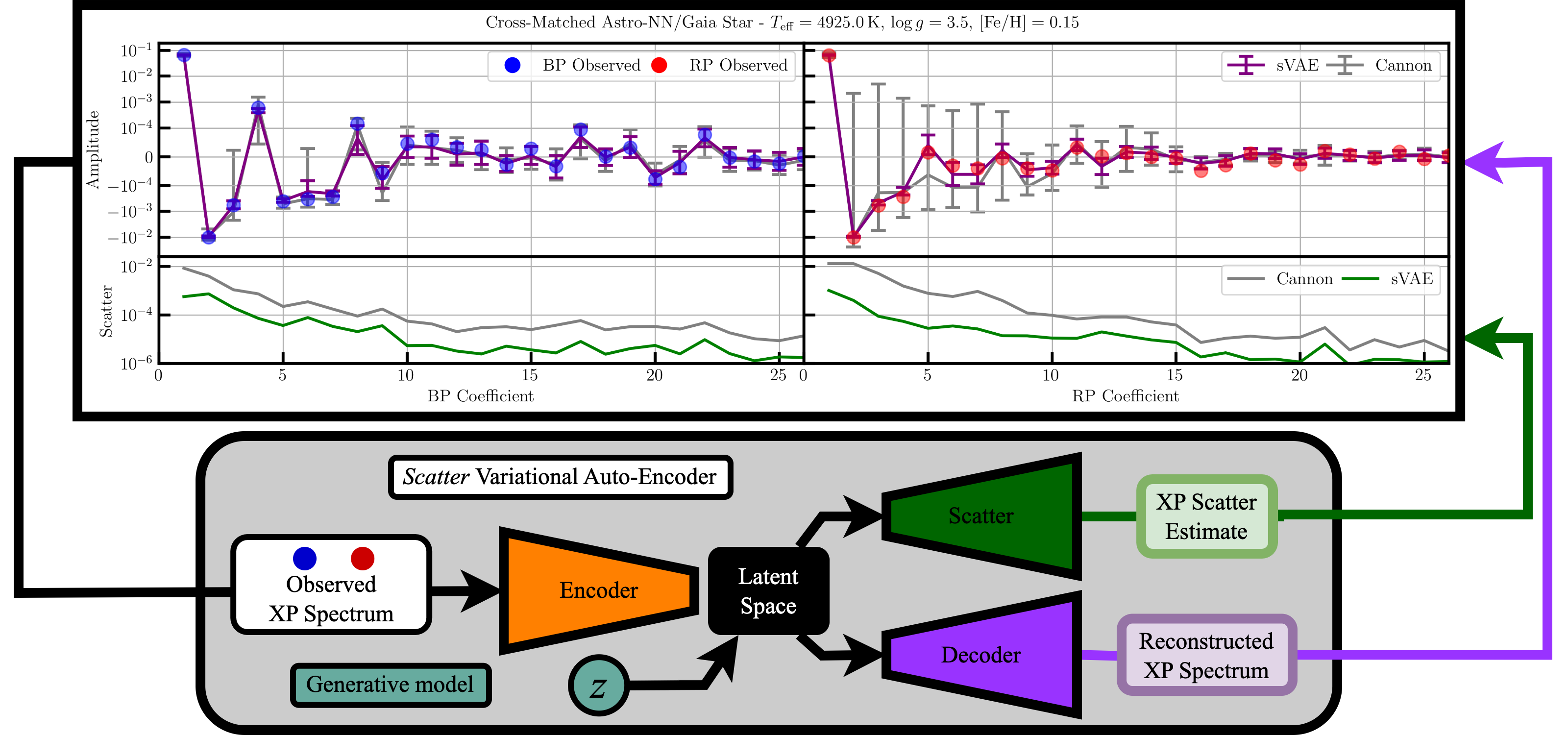
Figure 1: sVAE archictecture with an example spectrum. An observed XP spectrum is compressed by the encoder into the latent space. The latent space then generates an XP spectrum reconstruction and a scatter estimate. We compare our sVAE reconstruction to a Cannon model, which overestimates scatter in comparison to the sVAE. We do not explicitly display XP observational uncertainties as inputs since they are not propagated through the network, only factoring into our loss function (see Section 2.3). Note that the XP coefficient amplitudes are on a symmetric-log scale, and that error bars correspond to scatter and observational uncertainties added in quadrature.

2.1 Data

We use the XP coefficient spectra (XPCs) in this work. Here, we outline the important characteristics of the XPCs (see De Angeli et al. (2022); Montegriffo et al. (2022) for details). Gaia XP spectra deviate from traditional spectra in the sense that they are typically reported in Hermite polynomial space. Specifically, the BP and RP spectra are transformed from discrete wavelength-space into continuous coefficient-space: 110 coefficients which weight a set of Hermite polynomials (55 blue and 55 red coefficients). One can transform an XPCs into fluxes, and vice-versa, without loss of information. Indeed, Zhang et al. (2023) train their generative model in XP wavelength-space.

Before feeding coefficient XP spectra into our model, we perform the following data pre-processing: First, coefficients and errors are normalized by the mean flux in the Gaia G-band, removing the brightness dependence of XP coefficients. Second, we normalize the G-band flux normalized coefficients such that each coefficient has zero mean and unit variance. An XP spectrum is accompanied by a covariance matrix. In this work, we discard off-diagonal terms of the covariance matrix, treating coefficient errors as independent.

2.2 Scatter variational auto-encoder

We present a novel implementation of a variational auto-encoder (VAE), which we term a scatter variational auto-encoder (sVAE). Before describing our sVAE architecture, we briefly review the concept of a (V)AE.

An AE, which need not be variational, can be thought of as a non-linear generalization of Principal Component Analysis. An auto-encoder begins with an encoder which compresses input data, in our case a stellar spectrum, to a low-dimensional latent representation. A decoder then attempts to reconstruct the stellar spectrum from the latent representation. Ideally, this will allow the latent representation to learn key features which are shared across a set of stellar spectra. The variational nature of a VAE is added to an AE by upgrading the latent space from a collection of discrete points to a latent distribution $\mathcal{Z}$. The most popular VAE methodology is that of Kingma & Welling (2013), who encode input data onto an independent multivariate Gaussian distribution. The latent space can therefore be entirely characterized by a latent mean vector $\boldsymbol{\mu}$ and (log) variance vector $\log\boldsymbol{\sigma}^{2},$ with dimension (of the latent space) $n_{\mathcal{Z}}.$

We present the high-level architecture of our VAE in Figure 1. Our sVAE differs from a traditional VAE since, in addition to a decoder (purple) which estimates stellar spectra, we introduce a second ‘decoder’ which estimates intrinsic scatter on a star-by-star basis (green). Importantly, both the XP reconstruction and XP scatter estimate are generated from the same latent space (black). After discarding the encoder (orange) post-training, new XP coefficients (scatter) can be generated given an arbitrary latent space vector $\boldsymbol{z}$ (teal).

The input of our encoder is a (flux-normalized) XPCs. The XP coefficients are fed through three intermediate layers, composed of 80, 50 and 30 neurons, respectively. All intermediate layers are activated by the gaussian error linear unit (GELU). The latent parameters are then given by a linear transformation of the final intermediate layer. In this work, we have fixed the latent space to 6 dimensions, meaning the encoder produces 12 outputs (6 means and variances). Our decoder is the mirror image of our encoder, and takes as input a vector drawn from the latent distribution. We then reconstruct an XP spectrum, by feeding the latent vector through three intermediate layers analogous to the encoder, except in reverse order. Finally, a reconstruction of the 110 XP coefficients is produced with a linear transform. The scatter estimator has the exact same architecture as the decoder (while enforcing positivity). We emphasize that the weights and biases of the scatter estimator are entirely disconnected from the decoder. The scatter estimator does not produce an estimate of intrinsic scatter in the traditional sense; variance of the entire XP dataset assuming zero measurement error. Rather, the intrinsic scatter is ‘intrinsic’ to an individual star, because the scatter estimator produces different outputs on a star-by-star, or latent vector-by-latent vector basis. As such, it is more accurate to think of the intrinsic scatter as an error term which includes traditional intrinsic scatter, systematics, outliers, etc.

2.3 Training

After data pre-processing (see Section 2.1), we train our model on  500,000 XPCs for 100 epochs. Here, we select a subset of test Gaia XP stars which we cross-match with APOGEE to obtain stellar labels ($\sim 5\times 10^{5}$ spectra). We implement stochastic gradient descent (SGD) with momentum, with a batch size of 1024 and learning rate decay with an initial learning rate of $0.1.$ During training we aim to minimize the loss function

$$\mathcal{L}=\tilde{\chi}^{2}(\boldsymbol{x},\hat{\boldsymbol{x}},\boldsymbol{\sigma}_{x}^{2},\hat{\boldsymbol{\sigma}}_{s}^{2}) +D_{KL}(\boldsymbol{\mu},\log\boldsymbol{\sigma}^{2}).$$ (1)

$\tilde{\chi}^{2}$ is the reconstruction loss between an input XP spectrum $\boldsymbol{x}$ and a reconstructed spectrum $\hat{\boldsymbol{x}}$ (from the decoder), whilst incorporating observational uncertainties $\boldsymbol{\sigma}_{x}^{2}$ and intrinsic scatter $\hat{\boldsymbol{\sigma}}_{s}^{2}$ (from the scatter estimator). In Eq. (1), the $\tilde{\chi}^{2}$ term is given by

$$\tilde{\chi}^{2}(\boldsymbol{x},\hat{\boldsymbol{x}},\boldsymbol{\sigma}_{x}^{2},\hat{\boldsymbol{\sigma}}_{s}^{2})=\chi^{2}(\boldsymbol{x},\hat{\boldsymbol{x}},\boldsymbol{\sigma}_{x}^{2},\hat{\boldsymbol{\sigma}}_{s}^{2})+P(\boldsymbol{\sigma}_{x}^{2},\hat{\boldsymbol{\sigma}}_{s}^{2}).$$ (2)

The first term in Eq. (2) is the traditional (reduced) $\chi^{2},$ given by

$$\chi^{2}(\boldsymbol{x},\hat{\boldsymbol{x}},\boldsymbol{\sigma}_{x}^{2},\hat{\boldsymbol{\sigma}}_{s}^{2})=\frac{1}{2N}\sum_{i=1}^{N}\frac{(x_{i}-\hat{x}_{i})^{2}}{\sigma_{x,i}^{2}+\hat{\sigma}_{s,i}^{2}},$$ (3)

and the penalty term $P$ is given by

$$P(\boldsymbol{\sigma}_{x}^{2},\hat{\boldsymbol{\sigma}}_{s}^{2})=\frac{1}{2N}\sum_{i=1}^{N}\log\left(\sigma_{x,i}^{2}+\hat{\sigma}_{s,i}^{2}\right),$$ (4)

where we are summing over the $N=110$ XP coefficients. The reconstruction loss (Eq. (2)) can therefore be thought of as a modification to chi-square which incorporates an error term by effectively penalizing large scatter and/or uncertainties. The second term in Eq. (1) is the latent-space structure loss, for which we select the KL divergence (Kullback & Leibler, 1951), and is given by

$$D_{KL}(\boldsymbol{\mu},\log\boldsymbol{\sigma}^{2})=\frac{1}{2n_{\mathcal{Z}}}\sum_{i=1}^{n_{\mathcal{Z}}} \mu_{i}^{2}+e^{\left(\log\sigma_{i}^{2}\right)}-\left(1+\log\sigma_{i}^{2}\right),$$ (5)

where $\boldsymbol{\mu}$ ($\log\boldsymbol{\sigma}^{2}$) are the latent means (variances) and we are summing over latent space dimensions $n_{\mathcal{Z}}$. In the above form, $D_{KL}$ is not particularly intuitive. For the purposes of latent space structure loss, it can be thought as a distance for probability distributions. $D_{KL}=0$ if two distributions are identical and $D_{KL}>0$ otherwise. Hence, assuming a multivariate normal latent distribution, the KL divergence is a measure of the Gaussianity of the sVAE latent space.

3 Results

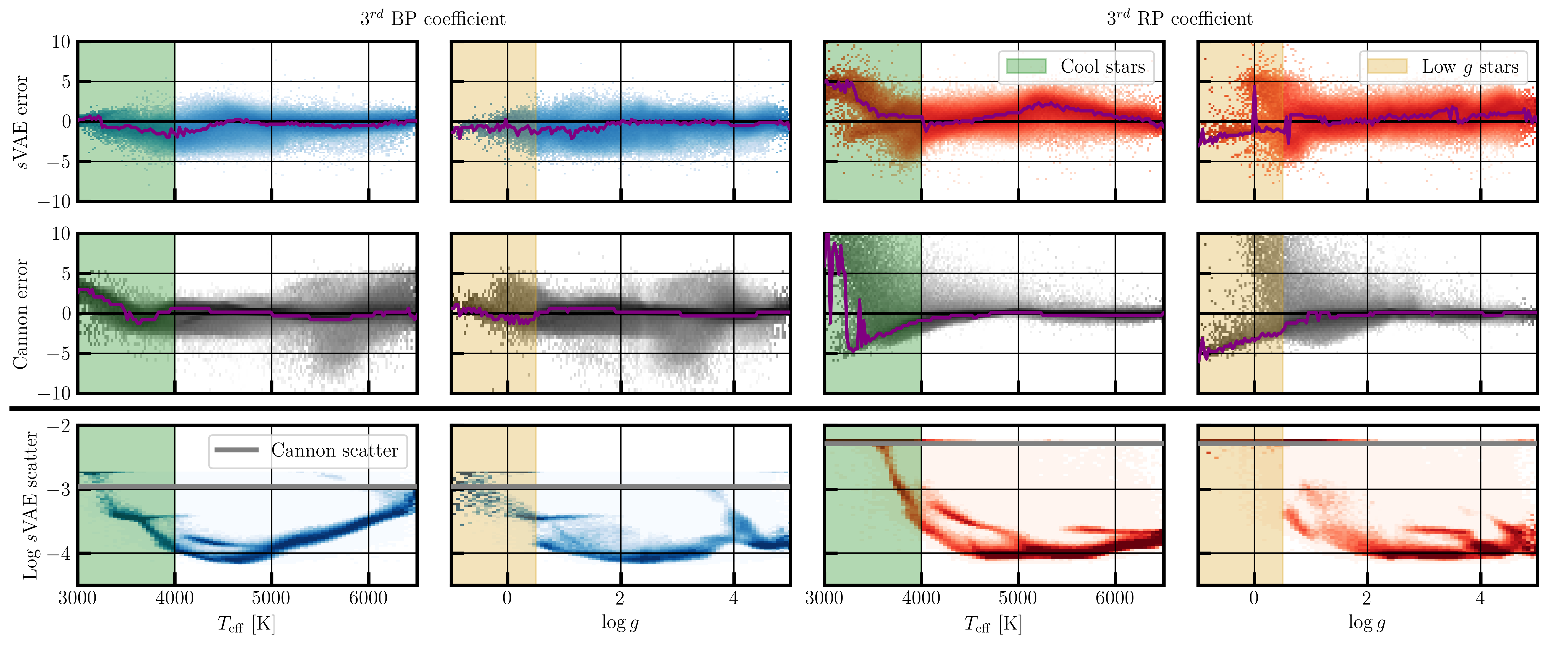
Figure 2: Normalized errors for the 3rd BP and RP coefficients, as functions of APOGEE stellar labels. sVAE errors (top) are compared to Cannon model errors (middle). sVAE star-by-star scatter (bottom) is compared to Cannon population scatter (grey). We highlight the improvement in performance with our sVAE for both cool stars (green) and low surface gravity stars (yellow). Purple lines indicate the mode normalized error as a function of stellar label.

We now present the results of our trained sVAE in comparison to a Cannon model. Reconstruction errors for our trained sVAE (normalized by observational uncertainty and intrinsic scatter added in quadrature) are presented in Figure 2. The Cannon model reconstructs an XP spectrum from stellar labels. We train the Cannon model on the same APOGEE/XP cross-match used for sVAE training in Section 2.3. Our unsupervised sVAE has three key advantages over existing supervised generative models:

1. Star-by-star intrinsic scatter estimation (and overall model flexibility) yields better XP reconstructions over all stellar parameter space.

2. Our trained sVAE accurately reconstructs stellar spectra in regions of stellar parameter space where supervised learning failed with (bad) stellar labels.

3. Our model covers far more of the XP parameter space than supervised learning.

First, in Figure 2, normalized errors for the sVAE clearly truncate at $\sim 5\sigma,$ whereas the Cannon errors can extend beyond $10\sigma.$ Although we only present the 3rd XP coefficients in Figure 2, the average, normalized errors for our trained sVAE across all XPCs in the APOGEE cross-match are only $2\%$ ($9\%$) larger than the Cannon model, for the first 10 BP (RP) coefficients. This is more impressive if we compare individual XP scatter to Cannon population scatter in the bottom row of Figure 2. The sVAE achieves the same accuracy as the Cannon model, with respect to normalized errors, while simultaneously having far smaller intrinsic scatter estimates (by up to 2 order of magnitude). The Cannon model overestimates intrinsic scatter, and by extension reduces normalized errors. In contrast, the lower (individual) scatter estimates of the sVAE allow an overall increase in reconstruction accuracy. In summary, our generically better XP reconstructions, relative to the Cannon model, can be attributed to $(i)$ inclusion of individual scatter estimation and $(ii)$ the flexibility of the generative function which relates the latent space to XPCs.

Second, the lack of reliance on stellar labels in our unsupervised approach is a significant advantage over supervised learning at the extrema of stellar parameter space. In Figure 2, we observe that our model is less susceptible to large errors at both the cool end of $T_{\rm eff}$ (green) and the low $g$ tail (yellow). In contrast, Cannon model errors blow up because supervised learning fails when bad stellar label estimates are used. Our sVAE avoids this shortcoming by swapping out stellar labels for a latent space as its generator.

Third, our unsupervised approach greatly increases ‘coverage’ of the XP parameter space, relative to supervised learning. The XP spectra contain rare stellar populations which are not well characterized by the current stellar label catalogs available for supervised learning. To illustrate this, we project both the entire XP/APOGEE cross-matched catalog and $10^{6}$ XP spectra (outside of the cross-match) into the sVAE latent space. This is visualized across two latent space dimensions in Figure 3. We observe that the XP/APOGEE cross-match covers significantly less latent space volume than the $10^{6}$ XP spectra without APOGEE labels. We compute the relative latent space volume difference by numerical integration and find $\Delta V/V_{\rm sup}\approx 30\%,$ meaning the $10^{6}$ unlabeled spectra cover 30% more latent space than the APOGEE cross-match. Extrapolating this to the entire 220 million XP spectra, our sVAE improves latent space coverage by approximately a factor of $220\times\frac{\Delta V}{100V_{\rm sup}}\approx 65$. We emphasize that this increase in latent space coverage is a crude approximation of the ‘breadth’ gained by our unsupervised approach. First, latent space coverage does not necessarily correspond to better stellar parameter space coverage (although it certainly can). Second, the sVAE is degenerate in the sense that the same model can learn different embeddings of the data, due to latent space symmetries. Therefore, the 65x factor we quote above is only qualitative. It serves to motivate the use of our sVAE: better latent space coverage, by roughly an order of magnitude, is a proxy for better information coverage over the XP dataset.

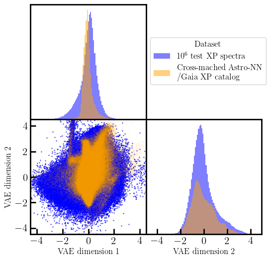
Figure 3: Latent space projection for the APOGEE/XP cross-matched catalog (orange) and $10^{6}$ unlabeled XP spectra (blue).

4 Conclusion & Future Work

We developed a novel deep, generative model: a scatter variational auto-encoder, and applied it to the Gaia XP spectra. We showed that our sVAE outperforms supervised learning (Cannon) in many respects. Most importantly, our unsupervised approach has the potential to close the stellar labels gap. Firstly, for XP spectra with stellar labels from previous spectroscopic surveys, our sVAE produces better reconstructions than supervised learning if stellar labels are poorly estimated. Second, our unsupervised model can cover the entire XP parameter space, whereas supervised learning is limited to only a small subset, because we swap out stellar labels for latent variables.

The evident shortcoming of trading stellar labels for latent labels is the inability to perform stellar label inference with our unsupervised model. Nevertheless, inference can be performed in the latent space to identify relative differences between stellar populations. Our sVAE, combined with existing supervised models (e.g. Zhang et al., 2023), will eventually yield an accurate, semi-supervised generative model for the entire Gaia XP data. Our approach is also promising for both outlier detection and identification of rare stellar populations. For example, we expect our approach will provide additional insights into the CEMP star catalog of Lucey et al. (2022) and aim to pursue this in future work.

References

- Abdurro’uf (2022) Abdurro’uf, e. The Seventeenth Data Release of the Sloan Digital Sky Surveys: Complete Release of MaNGA, MaStar, and APOGEE-2 Data. ApJS, 259(2):35, April 2022. doi: 10.3847/1538-4365/ac4414.
- De Angeli et al. (2022) De Angeli, F., Weiler, M., Montegriffo, P., Evans, D. W., Riello, M., Andrae, R., Carrasco, J. M., Busso, G., Burgess, P. W., Cacciari, C., Davidson, M., Harrison, D. L., Hodgkin, S. T., Jordi, C., Osborne, P. J., Pancino, E., Altavilla, G., Barstow, M. A., Bailer-Jones, C. A. L., Bellazzini, M., Brown, A. G. A., Castellani, M., Cowell, S., Delchambre, L., De Luise, F., Diener, C., Fabricius, C., Fouesneau, M., Fremat, Y., Gilmore, G., Giuffrida, G., Hambly, N. C., Hidalgo, S., Holland, G., Kostrzewa-Rutkowska, Z., van Leeuwen, F., Lobel, A., Marinoni, S., Miller, N., Pagani, C., Palaversa, L., Piersimoni, A. M., Pulone, L., Ragaini, S., Rainer, M., Richards, P. J., Rixon, G. T., Ruz-Mieres, D., Sanna, N., Sarro, L. M., Rowell, N., Sordo, R., Walton, N. A., and Yoldas, A. Gaia Data Release 3: Processing and validation of BP/RP low-resolution spectral data. arXiv e-prints, art. arXiv:2206.06143, June 2022. doi: 10.48550/arXiv.2206.06143.
- Gaia Collaboration (2022) Gaia Collaboration, e. Gaia Data Release 3: Summary of the content and survey properties. arXiv e-prints, art. arXiv:2208.00211, July 2022. doi: 10.48550/arXiv.2208.00211.
- Kingma & Welling (2013) Kingma, D. P. and Welling, M. Auto-Encoding Variational Bayes. arXiv e-prints, art. arXiv:1312.6114, December 2013. doi: 10.48550/arXiv.1312.6114.
- Kullback & Leibler (1951) Kullback, S. and Leibler, R. A. On information and sufficiency. The Annals of Mathematical Statistics, 22(1):79–86, 1951. ISSN 00034851. URL http://www.jstor.org/stable/2236703.
- Lucey et al. (2022) Lucey, M., Al Kharusi, N., Hawkins, K., Ting, Y.-S., Ramachandra, N., Beers, T. C., Lee, Y. S., Price-Whelan, A. M., and Yoon, J. Over 2.7 Million Carbon-Enhanced Metal-Poor stars from BP/RP Spectra in DR3. arXiv e-prints, art. arXiv:2206.08299, June 2022. doi: 10.48550/arXiv.2206.08299.
- Montegriffo et al. (2022) Montegriffo, P., De Angeli, F., Andrae, R., Riello, M., Pancino, E., Sanna, N., Bellazzini, M., Evans, D. W., Carrasco, J. M., Sordo, R., Busso, G., Cacciari, C., Jordi, C., van Leeuwen, F., Vallenari, A., Altavilla, G., Barstow, M. A., Brown, A. G. A., Burgess, P. W., Castellani, M., Cowell, S., Davidson, M., De Luise, F., Delchambre, L., Diener, C., Fabricius, C., Fremat, Y., Fouesneau, M., Gilmore, G., Giuffrida, G., Hambly, N. C., Harrison, D. L., Hidalgo, S., Hodgkin, S. T., Holland, G., Marinoni, S., Osborne, P. J., Pagani, C., Palaversa, L., Piersimoni, A. M., Pulone, L., Ragaini, S., Rainer, M., Richards, P. J., Rowell, N., Ruz-Mieres, D., Sarro, L. M., Walton, N. A., and Yoldas, A. Gaia Data Release 3: External calibration of BP/RP low-resolution spectroscopic data. arXiv e-prints, art. arXiv:2206.06205, June 2022. doi: 10.48550/arXiv.2206.06205.
- Ness et al. (2015) Ness, M., Hogg, D. W., Rix, H. W., Ho, A. Y. Q., and Zasowski, G. The Cannon: A data-driven approach to Stellar Label Determination. ApJ, 808(1):16, July 2015. doi: 10.1088/0004-637X/808/1/16.
- Rix et al. (2022) Rix, H.-W., Chandra, V., Andrae, R., Price-Whelan, A. M., Weinberg, D. H., Conroy, C., Fouesneau, M., Hogg, D. W., De Angeli, F., Naidu, R. P., Xiang, M., and Ruz-Mieres, D. The Poor Old Heart of the Milky Way. ApJ, 941(1):45, December 2022. doi: 10.3847/1538-4357/ac9e01.
- Wang et al. (2022) Wang, C., Huang, Y., Yuan, H., Zhang, H., Xiang, M., and Liu, X. The Value-added Catalog for LAMOST DR8 Low-resolution Spectra. ApJS, 259(2):51, April 2022. doi: 10.3847/1538-4365/ac4df7.
- Yan et al. (2022) Yan, H., Li, H., Wang, S., Zong, W., Yuan, H., Xiang, M., Huang, Y., Xie, J., Dong, S., Yuan, H., Bi, S., Chu, Y., Cui, X., Deng, L., Fu, J., Han, Z., Hou, J., Li, G., Liu, C., Liu, J., Liu, X., Luo, A., Shi, J., Wu, X., Zhang, H., Zhao, G., and Zhao, Y. Overview of the LAMOST survey in the first decade. The Innovation, 3:100224, March 2022. doi: 10.1016/j.xinn.2022.100224.
- Zhang et al. (2023) Zhang, X., Green, G. M., and Rix, H.-W. Parameters of 220 million stars from Gaia BP/RP spectra. arXiv e-prints, art. arXiv:2303.03420, March 2023. doi: 10.48550/arXiv.2303.03420.