Coexistence of Competing Microbial Strains under Twofold Environmental Variability and Demographic Fluctuations

Abstract

Microbial populations generally evolve in volatile environments, under conditions fluctuating between harsh and mild, e.g. as the result of sudden changes in toxin concentration or nutrient abundance. Environmental variability thus shapes the long-time population dynamics, notably by influencing the ability of different strains of microorganisms to coexist. Inspired by the evolution of antimicrobial resistance, we study the dynamics of a community consisting of two competing strains subject to twofold environmental variability. The level of toxin varies in time, favouring the growth of one strain under low drug concentration and the other strain when the toxin level is high. We also model time-changing resource abundance by a randomly switching carrying capacity that drives the fluctuating size of the community. While one strain dominates in a static environment, we show that species coexistence is possible in the presence of environmental variability. By computational and analytical means, we determine the environmental conditions under which long-lived coexistence is possible and when it is almost certain. Notably, we study the circumstances under which environmental and demographic fluctuations promote, or hinder, the strains coexistence. We also determine how the make-up of the coexistence phase and the average abundance of each strain depend on the environmental variability.

I Introduction

Microbial communities evolve in volatile environments that often fluctuate between mild and harsh conditions. For instance, the concentration of toxin and the abundance of nutrients in a community can suddenly and radically change [1, 2, 3, 4]. This results in environmental variability (EV) that shapes the population evolution [5, 6, 7, 8, 9, 10, 11, 12, 13]. In particular, EV greatly influences the ability of species to coexist [14, 15, 16, 17, 18, 19], which is a characteristic of key importance in biology and ecology, with direct applications in subjects of great societal concern [20, 21, 22, 23, 24, 25] like the maintenance of biodiversity in ecosystems [26, 27, 28, 29, 30, 31, 32, 33, 34] and the evolution of antimicrobial resistance (AMR) [35, 36, 37, 38, 39, 40].

In the absence of detailed knowledge about the time-variation of external factors, EV is generally modelled by means of noise terms affecting the species growth and/or death rates [41, 42, 43, 44, 45, 46, 47, 48, 49, 50, 51, 52, 53, 54, 26, 55, 56, 57, 58, 59, 60, 61, 62, 63, 64, 65, 66]. Demographic noise (DN) is another important source of fluctuations: it can lead to fixation, which is the phenomenon arising when one strain takes over the entire community. The effect of DN is significant in communities of small size, and becomes negligible in large populations [41, 42, 67, 68, 69]. Significantly, the time development of the size and composition of populations are often interdependent [70, 71, 72, 73, 74, 75, 76, 77, 78], with fluctuations of the population size modulating the strength of DN [57, 61, 62, 63, 65, 66, 79]. The interplay between EV and DN is crucial in shaping microbial communities, but the quantitative effects of their coupling are as yet still mostly unknown.

Environmental and demographic fluctuations play a crucial role in the evolution of AMR [38, 40, 60, 64, 13]. When treatments reduce a microbial community to a very small size, but fail to eradicate the microorganisms resistant to the drugs, resistant cells may replicate and restore infection, hence possibly leading to the spread of antibiotic resistance. Moreover, within a small population, demographic fluctuations may also lead to the extinction of resistant cells. Understanding how the coexistence of cells resistant and sensitive to antibiotics is affected by the joint effect of environmental variability and demographic fluctuations, and how the fraction of resistant cells varies with environmental conditions with the possibility of eradication, are thus central questions in the effort to understand the evolution of AMR [36, 38, 40, 13, 79].

It is worth noting that considerable efforts have recently been dedicated to study the mechanisms underpinning the coexistence of competing species under various scenarios, see e.g. [31, 32, 65, 34]. The influence of different kinds of variability (e.g. quenched disorder, heterogeneous rates, “spillover protection”) on species coexistence in ecosystems  exhibiting cyclic dominance [80, 59] has notably been investigated in [81, 47, 82, 83, 84, 85]. Here, inspired by the AMR evolution in a chemostat setup [65, 19], we study the eco-evolutionary dynamics of an idealised microbial community consisting of two competing strains subject to a time-varying level of toxin, with the growth of one strain favoured under low toxin level and a selective advantage to the other strain under high toxin level. We also assume that the resource abundance varies according to a time-switching carrying capacity that drives the fluctuating size of the community. In most of previous works, EV is either encoded in fluctuating growth rates, with the size or carrying capacity of the population kept constant  [41, 42, 43, 44, 45, 86, 47, 48, AMR13b, 49, 50, 51, 53, 54, 26, 55, 56, 58, 60, 64], or EV is modelled by a time-varying carrying capacity that affects the species death rates and drives the population size [57, 61, 62, 63, 66] (see also [65]). The distinctive feature of this study is therefore the twofold environmental variability accounting for fluctuations stemming from the variation of the toxin level and the switches of the carrying capacity resulting in the coupling of DN and EV; see Fig. 1.
As main results, we obtain the fixation-coexistence diagrams of the system, and these allow us to determine the environmental conditions under which long-lived coexistence of the strains is possible or certain, and when one strain dominates the other. We also analyse the make-up of the population when the strains coexist, and their average abundance.

The organisation of the paper is as follows: the model is introduced in Sec. II. Sec. III is dedicated to the study of the case with a constant carrying capacity (subject to a static or varying toxin level) by means of a mean-field analysis and a mapping onto a suitable Moran process. The twofold influence of time-varying fitness and carrying capacity on the coexistence and fixation of the species is analysed in Sec. IV. Sec. V is dedicated to the influence of the EV on the make-up of the coexistence phase and strains abundance. We present our conclusions in Sec. VI. Additional technical details are given in the appendix.

II Model

Figure 1: Cartoon of the model characterised by twofold EV. A microbial community consisting of two strains, denoted by $R$ (resistant, blue (charcoal), fitness $f_{R}$) and $S$ (sensitive, red (grey), fitness $f_{S}$), evolves in a time-varying environment, as illustrated by the arrows: the level of toxin, $\xi_{T}$, stochastically switches with rates $\nu_{T}^{\pm}$ (vertical arrows) between low ($\xi_{T}=+1$) and high ($\xi_{T}=-1$), and the amount of available resources, modelled by the carrying capacity $K(t)$, stochastically switches with rates $\nu_{K}^{\pm}$ (horizontal arrows) between scarce and abundant. The strain $R$ fares better than $S$ under high toxin level ($f_{R}>f_{S}$), while $S$ grows faster under low toxin level ($f_{R}<f_{S}$). The carrying capacity $K(t)=K_{+}$ when there are abundant resources, while $K(t)=K_{-}<K_{+}$ when available nutrients are scarce. The four environmental states characterising the twofold EV are indicated by the coloured background: striped / solid green (light grey) refers to low toxin level and scarce / abundant resources, while striped / solid red (grey) indicates high toxin level with scarce / abundant resources. See the text for the greyscale coding, and the table in Sec. SM1 of the appendix for detailed notations and definitions.

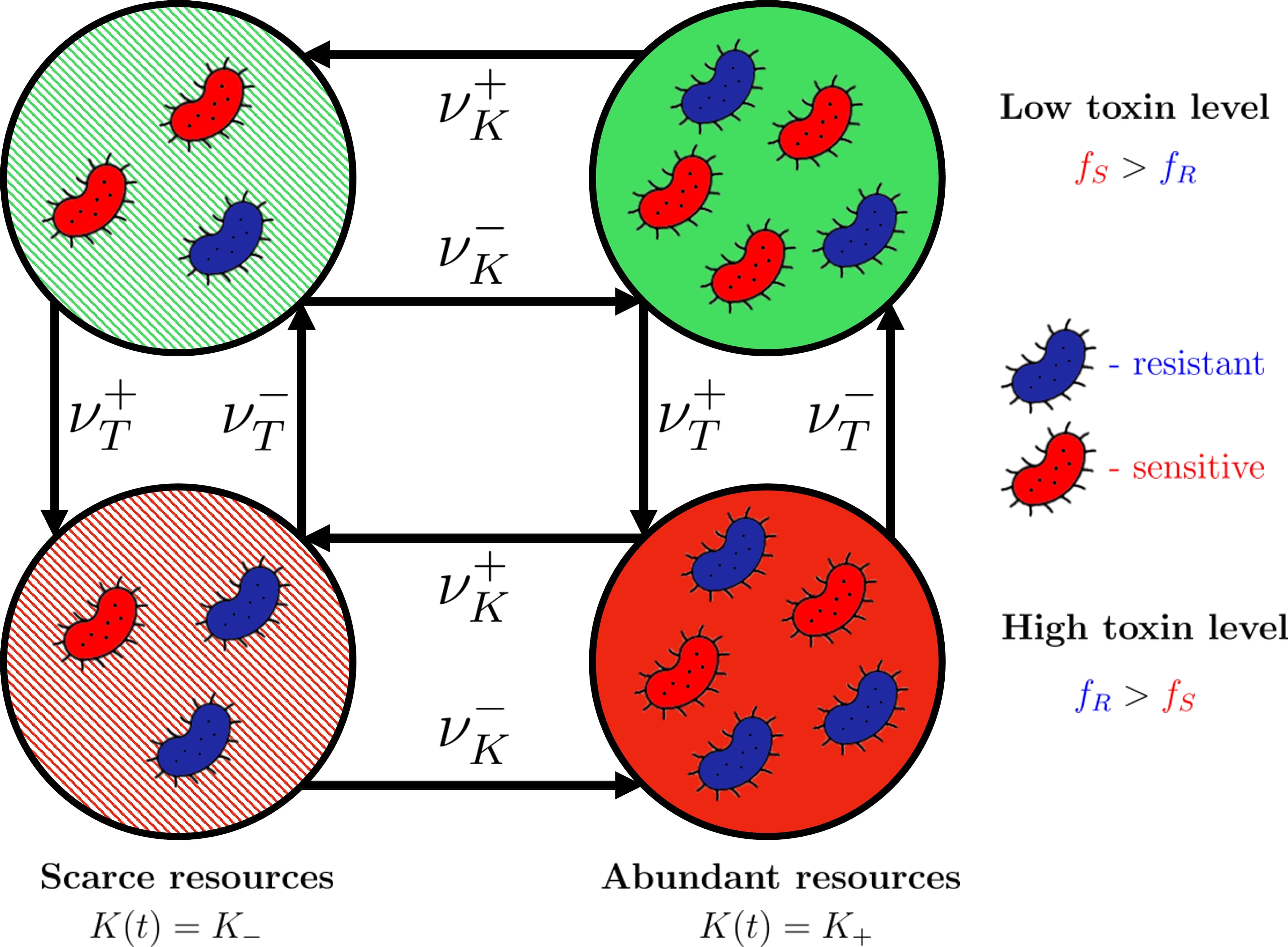
We consider a well-mixed population of fluctuating size $N(t)=N_{R}(t)+N_{S}(t)$ which, at time $t$, consists of $N_{R}$ bacteria of strain $R$ and $N_{S}$ of type $S$, which compete for the same resources. The former refers to a strain that pays a metabolic cost to be resistant to a certain toxin, and the latter to microorganisms sensitive to that toxin. Based on mounting evidence showing that microbial communities generally evolve in volatile environments [5, 6, 9, 12, 25], we study the eco-evolutionary dynamics of this population under twofold environmental variability: external conditions fluctuate between harsh and mild, and affect the level of toxin and resources that are available in the population; see Fig. 1.

For concreteness, we assume that the toxin is biostatic and reduces the growth rate of the sensitive strain, but does not affect the resistant bacteria [87, 88, 89]. In this setting, resistant $R$ bacteria have a constant fitness $f_{R}$, whereas the sensitive $S$ bacteria have an environment-dependent fitness $f_{S}(\xi_{T})$, where $\xi_{T}(t)$ is a time-varying environmental random variable encoding the toxin level: $\xi_{T}>0$ for the low toxin level and $\xi_{T}<0$ for the high toxin level. As in previous studies [91, 92, 29, 30, 93], we here consider

$$f_{R}=1\qquad\text{and}\qquad f_{S}=\exp(s\xi_{T}),$$

where $s>0$ denotes the selection bias favouring the strain $S$ when $\xi_{T}>0$, and strain $R$ when $\xi_{T}<0$. The parameter $s$ therefore encodes both the selection and strength of the environmental variability associated with the changes in toxin level ($T$-EV). As in many recent theoretical studies [57, 94, 91, 61, 63, 62, 65, 56], $T$-EV is here modelled by coloured dichotomous Markov noise (DMN) [95, 96, 97], so that $\xi_{T}\in\{-1,1\}$; see below. DMN is an important example of bounded noise [95, 96, 97, 56, 61, 63, 62, 65, 94], with finite correlation time, which allows us to efficiently model suddenly changing conditions occurring in bacterial life [86, 8, 71, 72, 19], like the environmental stress resulting from exposure to antibiotics [75, 10, 11]. In this context, DMN, that is easy to simulate accurately and whose relationships with more complex forms of noise have been studied (see Sec. SM4 in the appedix and  [95, 96, 66]), provides us with mathematically-amenable models that can be regarded as the theoretical counterparts of commonly-used laboratory experimental chemostat set-ups [8, 19, 13, 11].

The environmental effect on the level of nutrients ($K$-EV), fluctuating between scarcity and abundance, is modelled by a binary switching carrying capacity $K(t)\in\{K_{-},K_{+}\}$ that is driven by the binary random variable (also following a DMN process) $\xi_{K}(t)\in\{-1,1\}$. The state $\xi_{K}=-1$ thus corresponds to a harsh state with scare resources, where the carrying capacity is $K_{-}$, whereas nutrients are abundant in the mild state $\xi_{K}=+1$ where the carrying capacity is $K_{+}>K_{-}\gg 1$. As in [57, 61, 63, 62, 65, 66], this is encoded in the time-switching carrying capacity

$$K(t)=\frac{1}{2}\left[K_{+}+K_{-}+\xi_{K}(t)(K_{+}-K_{-})\right],$$ (1)

which, with $K_{0}\equiv\frac{K_{+}+K_{-}}{2}$ and $\gamma\equiv\frac{K_{+}-K_{-}}{2K_{0}}$, can conveniently be written as

$$K(t)=K_{0}[1+\gamma\xi_{K}(t)].$$

This randomly switching carrying capacity drives the population size $N(t)$ and is hence responsible for its fluctuations, with $K(t)\gg 1$ ensuring that the population dynamics is never solely dominated by demographic fluctuations. It is worth noting the choice of $\xi_{K}$ as a DMN ensures that the carrying capacity is always bounded and physical, i.e. $K(t)\in\{K_{-},K_{+}\}$ and $K(t)>0$, which is not the case if EV is modelled by unbounded (e.g. Gaussian) noise, see Sec. SM4 in the appendix.

The population thus evolves under twofold EV encoded in the environmental states ${\xi_{T}(t),\xi_{K}(t)}$, see Fig. 1, subject to time switching according to the reactions

$$\xi_{\alpha}=+1\xrightarrow{\nu_{\alpha}^{+}}-1,\hskip 14.22636pt\text{and}\hskip 14.22636pt\xi_{\alpha}=-1\xrightarrow{\nu_{\alpha}^{-}}+1,$$ (2)

where $\nu_{\alpha}^{\pm}$ are the switching rates of the $\alpha$-DMN, with $\alpha\in\{T,K\}$ indicating the relevant environmental noise. It is also useful to define the average switching rate $\nu_{\alpha}$ and switching bias $\delta_{\alpha}$ for each $\alpha$-DMN as

$$\nu_{\alpha}\equiv\frac{\nu_{\alpha}^{-}+\nu_{\alpha}^{+}}{2}\hskip 14.22636pt\text{and}\hskip 14.22636pt\delta_{\alpha}\equiv\frac{\nu_{\alpha}^{-}-\nu_{\alpha}^{+}}{2\nu_{\alpha}},$$

such that $\nu_{\alpha}^{\pm}\equiv\nu_{\alpha}(1\mp\delta_{\alpha})$. This means that $\delta_{T}>0$ corresponds to a bias towards low toxin level (mild $T$ state, $\xi_{T}=+1$) favouring the $S$ strain, whereas $\delta_{T}<0$ indicates a bias towards high toxin level (harsh $T$ state, $\xi_{T}=-1$) where the growth of $S$ is hampered and the spread of $R$ is favoured, see Fig. 1. Similarly, $\delta_{K}>0$ corresponds to bias towards the environmental state rich in nutrients (where $K=K_{+}$), while $\delta_{K}<0$ is associated with a bias towards an environment where nutrients are scarce ($K=K_{-}$). In all cases, we consider $\alpha$-DMN at stationarity, where $\xi_{\alpha}=\pm 1$ with probability $(1\pm\delta_{\alpha})/2$, yielding the average $\left\langle\xi_{\alpha}\right\rangle=\delta_{\alpha}$ and autocovariance (autocorrelation up to a constant) $\left\langle\xi_{\alpha}(t)\xi_{\alpha}(t^{\prime})\right\rangle-\left\langle\xi_{\alpha}(t)\right\rangle\left\langle\xi_{\alpha}(t^{\prime})\right\rangle=(1-\delta_{\alpha}^{2})\exp(-2\nu_{\alpha}|t-t^{\prime}|)$, where $\left\langle\cdot\right\rangle$ denotes the $\alpha$-DMN ensemble average. We notice that the correlation time of the ${\alpha}$-DMN, $1/(2\nu_{\alpha})$, is half of the inverse of the average switching rate of $\xi_{\alpha}$ [95, 96, 97]. From Eq. equation 1, we find that the average carrying capacity is $\left\langle K\right\rangle=K_{0}(1+\gamma\delta_{K})$ and the variance of $K(t)$ is $(K_{0}\gamma)^{2}(1-\delta_{K}^{2})$, with the amplitude of $K$-EV thus scaling as $K_{0}\gamma$, while the variance and amplitude of the $T$-EV increase with $s$; see Sec. SM2 the appendix.

For concreteness, we here assume that $\xi_{T}$ and $\xi_{K}$ are totally uncorrelated. In our motivating example, this corresponds to the reasonable assumption that nutrient and antibiotic uptake are independent processes. The case where $\xi_{T}$ and $\xi_{K}$ are fully correlated or fully anti-correlated, with $\xi_{T}=\xi_{K}=\xi$ or $\xi_{T}=-\xi_{K}=\xi$, where $\xi$ is a single DMN process, is briefly discussed in Sec. SM8 of the appendix.

The system considered here best translates to a chemostat setup whereby toxin and nutrient levels can be maintained at a constant level through time and switched via changing concentrations of medium coming into the system [65, 19]. The switch $\xi_{T}\to-\xi_{T}$ with $\xi_{T}=-1$ can thus be envisioned as corresponding to switching the concentration of an antibiotic drug from above the minimum inhibitory concentration (MIC), where the growth of the sensitive strain is hampered, to a concentration below the MIC where the $S$ strain can spread at the expense of $R$ [36, 38, 64].

At time $t$ the fraction of $R$-types in the system is $x(t)\equiv\frac{N_{R}(t)}{N(t)}$ and the average population fitness is $\overline{f}(x,\xi_{T})\equiv x+(1-x)\exp(s\xi_{T})$, which depends on the population composition $x$ and the toxin state $\xi_{T}$, . We assume that mutation rates between strains are negligible, and seek to characterise the population dynamics by the evolution of its size and composition according to the multivariate birth-death process [98, 99, 100]

$$N_{R/S}\xrightarrow{T_{R/S}^{+}}N_{R/S}+1\hskip 5.69046pt\text{and}\hskip 5.69046ptN_{R/S}\xrightarrow{T_{R/S}^{-}}N_{R/S}-1,$$ (3)

where the time-dependent birth and death transition rates are respectively

$$T_{R/S}^{+}=\frac{f_{R/S}}{\overline{f}}N_{R/S}\hskip 5.69046pt\text{and}\hskip 5.69046ptT_{R/S}^{-}=\frac{N}{K}N_{R/S}.$$ (4)

The per-capita birth rates $f_{R/S}/\overline{f}$ (where we normalise with $\overline{f}$ in line with the standard Moran process [101, 67, 68, 41, 69]) thus vary with the toxin level and population composition, while the logistic-like per-capita death rate $N/K$ varies with nutrient level and population size. With $\mathbf{N}\equiv(N_{R},N_{S})$, the master equation giving the probability $P(\mathbf{N},\xi_{T},\xi_{K},t)$ for the population to consist of $N_{R}$ and $N_{S}$ bacteria of type $R$ and $S$, respectively, in the environmental state $(\xi_{T},\xi_{K})$ at time $t$ is

$$\frac{\partial P(\mathbf{N},\xi_{T},\xi_{K},t)}{\partial t}=\left(\mathbb{E}_{R}^{-}-1\right)\left[T^{+}_{R}P(\mathbf{N},\xi_{T},\xi_{K},t)\right]$$ (5)

$$+\left(\mathbb{E}_{S}^{-}-1\right)\left[T^{+}_{S}P(\mathbf{N},\xi_{T},\xi_{K},t)\right]$$

$$+\left(\mathbb{E}_{R}^{+}-1\right)\left[T^{-}_{R}P(\mathbf{N},\xi_{T},\xi_{K},t)\right]$$

$$+\left(\mathbb{E}_{S}^{+}-1\right)\left[T^{-}_{S}P(\mathbf{N},\xi_{T},\xi_{K},t)\right]$$

$$+\nu_{T}^{-\xi_{T}}P(\mathbf{N},-\xi_{T},\xi_{K},t)-\nu_{T}^{\xi_{T}}P(\mathbf{N},\xi_{T},\xi_{K},t)$$

$$+\nu_{K}^{-\xi_{K}}P(\mathbf{N},\xi_{T},-\xi_{K},t)-\nu_{K}^{\xi_{K}}P(\mathbf{N},\xi_{T},\xi_{K},t),$$

where $\mathbb{E}^{\pm}_{R/S}$ are shift operators such that $\mathbb{E}^{\pm}_{R}f(N_{R},N_{S},\xi_{T},\xi_{K},t)=f(N_{R}\pm 1,N_{S},\xi_{T},\xi_{K},t)$, and $\nu_{\alpha}^{\xi_{\alpha}}\equiv\nu_{\alpha}^{\pm}$ when $\xi_{\alpha}=\pm 1$. We note that $P(\mathbf{N},\xi_{T},\xi_{K},t)=0$ whenever $N_{R}<0$ or $N_{S}<0$, and the last two lines on the right-hand-side of Eq. LABEL:eq:ME account for the random environmental switching of toxin ($\xi_{T}\to-\xi_{T}$) and carrying capacity ($\xi_{K}\to-\xi_{K}$). The dynamics encoded by the multivariate master equation Eq. (LABEL:eq:ME) can be simulated exactly by a stochastic algorithm as explained in [102, 103], see Sec. SM4 in the appendix. Since $T^{\pm}_{R/S}=0$ whenever $N_{R/S}=0$, there is extinction of $R$ and fixation of $S$ ($N_{R}=0,N=N_{S}$), or fixation of $R$ and extinction of $S$ ($N_{S}=0,N=N_{R}$). When one strain fixates and replaces the other, the population composition no longer changes while its size continues to fluctuate. Fixation of one strain and extinction of the other is expected when strains compete for the same resources (competitive exclusion principle), and always occur in a finite population even when its size fluctuates [57, 61, 63]. In stark contrast, here we show that environmental fluctuations can lead to the long-lived coexistence of competing species and nontrivially shape the abundance distribution of both strains.

The notation and definitions of the model parameters and physical quantities of interest are conveniently summarised in the table of Sec. SM1 in the appendix.

III Constant carrying capacity: mean-field analysis and Moran process

Since $\xi_{T}$ and $\xi_{K}$ are independent, it is useful to first consider the case of a constant carrying capacity, with environmental variability stemming only from the fluctuations of the toxin level in the birth rates of Eq. (4).

In this section, we thus assume that the carrying capacity is constant and large: $K(t)=K_{0}\gg 1$. After a short transient the population size fluctuates about $K_{0}$, with $N\approx K_{0}$. When $K_{0}\gg 1$, we can approximate the population size by $N=K_{0}$ and make analytical progress by using the well-known results of the Moran process [101, 67, 68, 41, 69]. In this approximation, the population is kept constant, which requires the simultaneous birth and death of individuals of either species, and the population evolves according to a fitness-dependent Moran process [57, 61, 62, 63], defined in terms of Eqs. equations 3 and 4 by the reactions

$$(N_{R},N_{S}) \xrightarrow{\widetilde{T}_{R}^{+}}(N_{R}+1,N_{S}-1),$$ (6)

$$(N_{R},N_{S}) \xrightarrow{\widetilde{T}_{R}^{-}}(N_{R}-1,N_{S}+1),$$

corresponding, respectively, to the simultaneous birth of an $R$ and death of an $S$ with rate $\widetilde{T}_{R}^{+}$, and death of an $R$ and birth of an $S$ with rate $\widetilde{T}_{R}^{-}$, where

$$\widetilde{T}_{R}^{+} \equiv\frac{T_{R}^{+}T_{S}^{-}}{N}=Nx(1-x)\frac{f_{R}}{\overline{f}(t)},$$ (7)

$$\widetilde{T}_{R}^{-} \equiv\frac{T_{R}^{-}T_{S}^{+}}{N}=Nx(1-x)\frac{f_{S}(t)}{\overline{f}(t)}.$$

III.1 Mean-field analysis

We now consider the case where $N=K_{0}\to\infty$, and thus ignore demographic fluctuations. In this case, the population composition evolves according to the mean-field equation [98]:

$$\dot{x}=\frac{\widetilde{T}_{R}^{+}-\widetilde{T}_{R}^{-}}{N}=x(1-x)\left(\frac{1-e^{s\xi_{T}}}{x+(1-x)e^{s\xi_{T}}}\right),$$ (8)

where the dot denotes the time derivative. It is important to notice that, owing to environmental noise $\xi_{T}$, Eq. (8) is a mean-field stochastic differential equation that defines a so-called “piecewise deterministic Markov process” (PDMP) [105, 56, 61, 57, 63]. According to this PDMP, after a switch to an environmental state $\xi_{T}$, $x$ evolves deterministically with Eq. (8) and a fixed value of $\xi_{T}$, until a switch $\xi_{T}\to-\xi_{T}$ occurs, see Sec. V.1.

We consider Eq. (8) in the regimes of (i) low, (ii) high, and (iii) intermediate switching rate $\nu_{T}$:
(i) Under low switching rate, $\nu_{T}\to 0$, the population settles in its final state without experiencing any $T$-switches. In this regime, the population reaches its final state in its initial toxin level $\xi_{T}(0)$, i.e. $\xi_{T}(0)=\xi_{T}(\infty)=\pm 1$ with probability $(1\pm\delta_{T})/2$. In this regime, Eq. (8) thus boils down to

$$\dot{x}=\begin{cases}-\frac{x(1-x)(e^{s}-1)}{x+(1-x)e^{s}}&\text{ with probability }\frac{1+\delta_{T}}{2}\\ \frac{x(1-x)(1-e^{-s})}{x+(1-x)e^{-s}}&\text{ with probability }\frac{1-\delta_{T}}{2}.\end{cases}$$ (9)

Since $s>0$, with a probability $(1+\delta_{T})/2$ we have $\xi_{T}(0)=\xi_{T}(\infty)=+1$ and $x\to 0$ ($R$ vanishes), while with a probability $(1-\delta_{T})/2$ we have $\xi_{T}(0)=\xi_{T}(\infty)=-1$ and $x\to 1$ ($S$ vanishes). In either case, the mean-field dynamics are characterised by the dominance of one of the strains. Therefore, in the absence of demographic fluctuations, there is never long-lived coexistence of the strains $R$ and $S$ under low switching rate of the toxin level.
(ii) Under high switching rate, $\nu_{T}\gg 1$, the population experiences a large number of $T$-switches before relaxing into its final state; see below. In this case the $T$-DN self-averages [57, 61, 63, 66, 53, 29] and we are left with a Moran process defined by the effective rates $\widetilde{T}_{R}^{\pm}\to\left\langle\widetilde{T}_{R}^{\pm}\right\rangle$ obtained by averaging $\xi_{T}$ over its stationary distribution, yielding

$$\left\langle\widetilde{T}_{R}^{+}\right\rangle =\frac{Nx(1-x)}{2}\left(\frac{1+\delta_{T}}{x+(1-x)e^{s}}+\frac{1-\delta_{T}}{x+(1-x)e^{-s}}\right),$$ (10)

$$\left\langle\widetilde{T}_{R}^{-}\right\rangle =\frac{Nx(1-x)}{2}\left(\frac{(1+\delta_{T})e^{s}}{x+(1-x)e^{s}}+\frac{(1-\delta_{T})e^{-s}}{x+(1-x)e^{-s}}\right).$$

When $N\to\infty$, the mean-field (MF) rate equation associated with this effective Moran process thus reads [68, 98, 99]:

$$\dot{x} =\frac{\left\langle\widetilde{T}_{R}^{+}\right\rangle-\left\langle\widetilde{T}_{R}^{-}\right\rangle}{N}$$ (11)

$$=\frac{x(1-x)}{2}\left[\frac{(1+\delta_{T})(1-e^{s})}{x+(1-x)e^{s}}+\frac{(1-\delta_{T})(1-e^{-s})}{x+(1-x)e^{-s}}\right],$$

where the right-hand-side (RHS) can be interpreted as the RHS of Eq. (8) averaged over $\xi_{T}$. In addition to the trivial fixed points $x=0,1$, Eq. (11) admits a coexistence equilibrium

$$x^{*}=\frac{1}{2}-\frac{\delta_{T}}{2}\coth{\frac{s}{2}},$$ (12)

when $-\tanh{\frac{s}{2}}<\delta_{T}<\tanh{\frac{s}{2}}$. This equilibrium stems from the $T$-DMN and thus is a fluctuation-induced coexistence point. In the case of large $s$ we have that $\coth{\frac{s}{2}}\rightarrow 1$, and $x^{*}$ exists ($0<x^{*}<1$) for all values of $\delta_{T}$. Since $\left.\frac{\text{d}\dot{x}}{\text{d}x}\right|_{x^{*}}=-\frac{4}{1-\delta_{T}^{2}}\tanh^{2}\left(\frac{s}{2}\right)\left(1-x^{*}\right)<0$

is negative, linear stability analysis reveals that $x^{*}$ is the sole asymptotically stable equilibrium of Eq. (11) when it exists ($x=0,1$ are thus unstable). When $s\ll 1$, $\coth{\frac{s}{2}}\rightarrow\frac{2}{s}$, and $x^{*}$ exists only for $-\frac{s}{2}<\delta_{T}<\frac{s}{2}$. This means that for $s\ll 1$, coexistence is essentially possible only under symmetric switching ($\delta_{T}=0$), see Sec. SM2 the appendix. In what follows, we focus on the less restrictive case $s={\cal O}(1)$, for which coexistence is possible for a broad range of parameters $(\nu_{T},\delta_{T})$.

(iii) In the regime of intermediate switching rate, where $\nu_{T}\sim 1$, the population experiences a finite number of $T$-switches prior to settling in its final state. Depending on this number, as well as the selection strength $s$ and the population size, the dynamics may be closer to either the low or high $\nu_{T}$ regime, with dominance or coexistence possible but, in general, not certain; see Fig. 3 below.

III.2 Finite populations - fixation and long-lived coexistence

Figure 2: $R$ fixation probability $\phi$ and MFT $\tau$ under constant carrying capacity and $T$-EV. Symbols are from stochastic simulations ($10^{3}$ realisations) with carrying capacity $K_{0}$ (and non-constant $N$), and full black lines are for the Moran approximation with $N=K_{0}$, based on Eq. (III.2) (a) and Eq. (III.2) (b,c). (a) $\phi$ against $\nu_{T}$, for $\delta_{T}=-0.9$ ($\times$), $-0.5$ ($\bigcirc$), $0$ ($\bigtriangledown$), $0.5$ ($\bigtriangleup$), $0.9$ ($\lozenge$), from top to bottom, with $s=0.3$ and $K_{0}=50$. Red dashed lines are predictions of Eq. (III.2) and Eq. (14). (b) $\tau$ against $\nu_{T}$, for $\delta_{T}=0$ ($\bigtriangledown$), $0.3$ ($\square$), $0.5$ ($\bigtriangleup$) from top to bottom, with $s=0.1$ and $K_{0}=500$. Any bias $\delta_{T}\neq 0$, reduces $\tau$. Error bars (dark grey) are overlaid for the case $\delta_{T}=0$ and almost indistinguishable from the symbols; see text and SM4 the appendix. Red dashed lines are analytical predictions in the limiting regimes $\nu_{T}\to 0,\infty$ (Eq. (S4) the appendix with same time-averaging process of rates as in Sec. III.1). (c)  $\tau$ against $K_{0}$ under fast $T$-EV in the coexistence regime for $\delta_{T}=0$, $s=0.1$ (

$\bigtriangleup$

) and $s=0.3$ (

$\bigtriangleup$

). Here, there is long-lived coexistence of the strains at the (meta-)stable equilibrium $x^{*}=x_{0}=0.5$ prior to fixation. The MFT grows exponentially when $K_{0}s^{2}\gg 1$, see Sec. SM2 the appendix. Red dashed lines show the analytical predictions for the MFT when $\nu_{T}\to\infty$ (Eq. (S4) the appendix with Eq. (10)), compared with the predictions of Eq. (III.2) (black lines) and simulation results (markers) for $\nu_{T}=100$.

From the MF analysis, we have found that when $N\to\infty$ species coexistence is feasible under fast $T$-EV switching, whereas only $R$ or $S$ dominance occurs under slow switching. We now study how these results nontrivially morph when the population is fixed and finite.

Since the model is defined as a finite Markov chain with absorbing boundaries, see Eqs. (6) and (7), its final state unavoidably corresponds to the fixation of one strain and the extinction of the other, i.e. the population eventually ends up in either the state $(N_{R},N_{S})=(N,0)$ or $(N_{R},N_{S})=(0,N)$  [100, 101, 68, 41]. This means that, strictly, the finite population does not admit stable coexistence: when it exists, $x^{*}$ is metastable [106, 107, 108]. In fact, while it is guaranteed that eventually only one of the strains will finally survive, fixation can occur after a very long time and can follow a long-term coexistence of the strains, as suggested by the MF analysis of the regime with $\nu_{T}\gg 1$. It is thus relevant to study under which circumstances there is long-lived coexistence of the strains.

The evolutionary dynamics is characterised by the fixation probability of the strain $R$, here denoted by $\phi$. This is the probability that a population, consisting initially of a fraction $x_{0}$ of $R$ bacteria, is eventually taken over by the strain $R$.
A related quantity is the unconditional mean fixation time (MFT), here denoted by $\tau$, which is the average time for the fixation of either species to occur.

In what follows, we study how the $R$ fixation probability $\phi(\nu_{T})$ and the MFT $\tau(\nu_{T})$ vary with the average switching rate of the $T$-EV for different values of $K_{0}$, $\delta_{T}$, and $s$ (treated as parameters), and determine when there is long-lived coexistence of the strains.

In the limits $\nu_{T}\to 0,\infty$, we can use the well-known properties of the Moran model [101, 41, 69] to obtain $\phi(\nu_{T})$ and $\tau(\nu_{T})$ from their Moran approximation (MA) counterparts, denoted by $\phi_{\rm MA}(N)$ and $\tau_{\rm MA}(N)$, which are respectively the $R$ fixation probability and mean fixation time in the associated Moran process for a population of constant size $N$; see Sec. SM3 the appendix.

For a given initial resistant fraction, the fixation probability in the slow-switching regime, $\phi(\nu_{T}\to 0)$ is obtained by averaging $\phi_{{\rm MA}}(N){\big{|}}_{\xi_{T}}$, denoting the $R$ fixation probability in the realm of the MA in static environment $\xi_{T}$, over the stationary distribution of $\xi_{T}$ [57, 61, 63, 66]:

$$\phi(\nu_{T}\to 0) =\left(\frac{1+\delta_{T}}{2}\right)\phi_{{\rm MA}}(N){\big{|}}_{\xi_{T}=+1}$$

$$+\left(\frac{1-\delta_{T}}{2}\right)\phi_{{\rm MA}}(N){\big{|}}_{\xi_{T}=-1}.$$ (13)

When $N\gg 1$ and $\xi_{T}=+1$ the strain $S$ is always favoured and $\phi_{{\rm MA}}(N){\big{|}}_{\xi_{T}=+1}\approx 0$, whereas $R$ is favoured when $\xi_{T}=-1$ and in this case $\phi_{{\rm MA}}(N){\big{|}}_{\xi_{T}=-1}\approx 1$. Since $\xi_{T}(0)=-1$ with probability $(1-\delta_{T})/2$, this coincides with the $R$ fixation probability: $\phi(\nu_{T}\to 0)\approx(1-\delta_{T})/2$. The probability that $S$ fixates when $\nu_{T}\to 0$ is thus $1-\phi(\nu_{T}\to 0)\approx(1+\delta_{T})/2$

In the fast-switching regime the fixation probability is that of the Moran process defined by the effective rates in Eq. (10). Using Eq. (10) with $x=n/N$, we thus find [41, 101]:

$$\phi(\nu_{T}\to\infty)=\frac{1+\sum_{k=1}^{Nx_{0}-1}\prod_{n=1}^{k}\frac{\left\langle\widetilde{T}_{R}^{-}\left(n/N\right)\right\rangle}{\left\langle\widetilde{T}_{R}^{+}\left(n/N\right)\right\rangle}}{1+\sum_{k=1}^{N-1}\prod_{n=1}^{k}\frac{\left\langle\widetilde{T}_{R}^{-}\left(n/N\right)\right\rangle}{\left\langle\widetilde{T}_{R}^{+}\left(n/N\right)\right\rangle}};$$ (14)

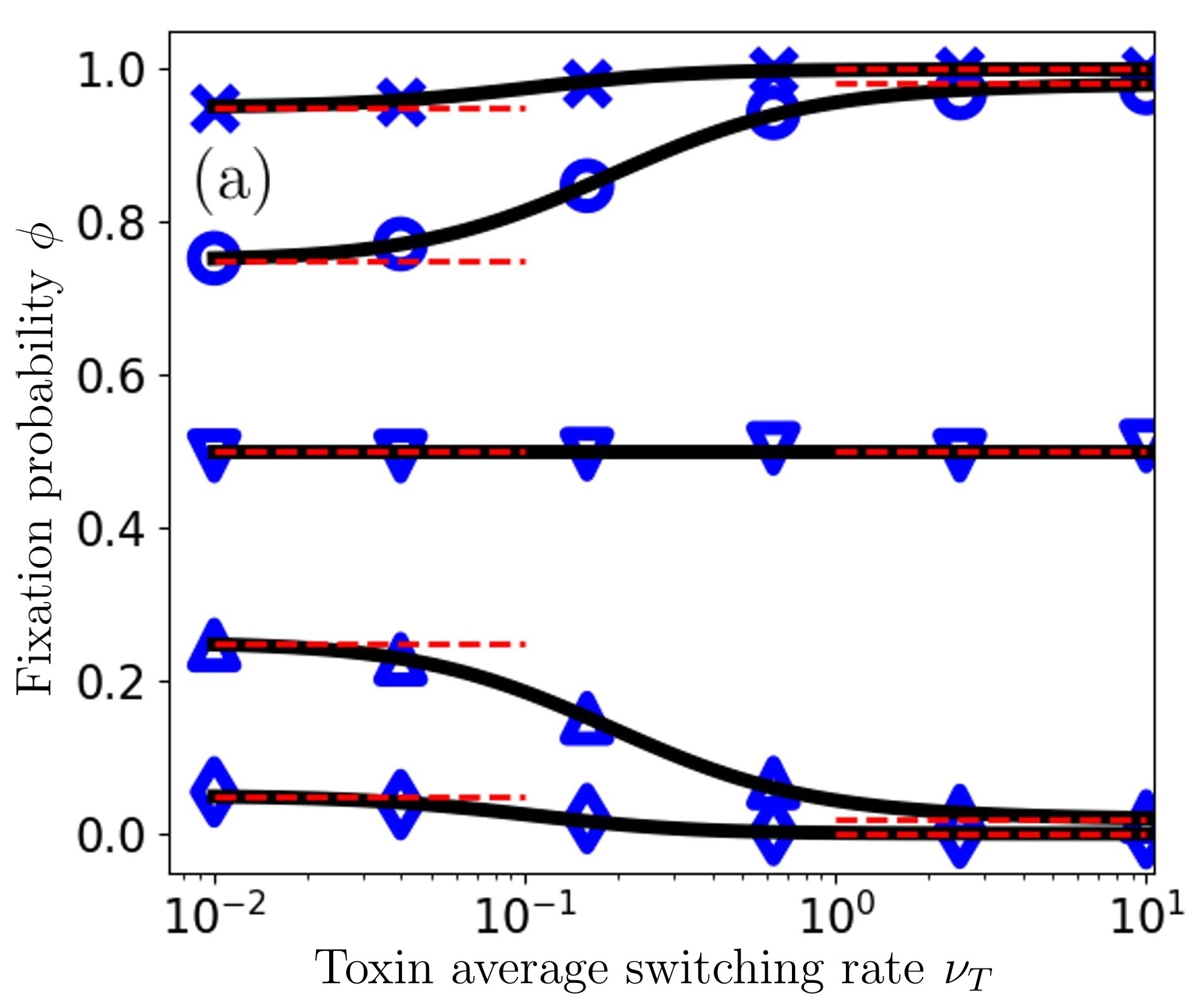
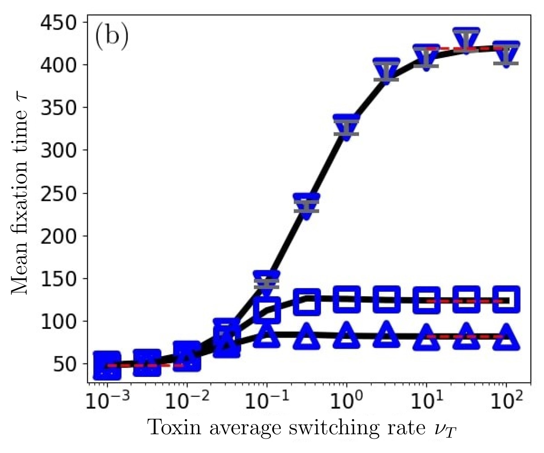
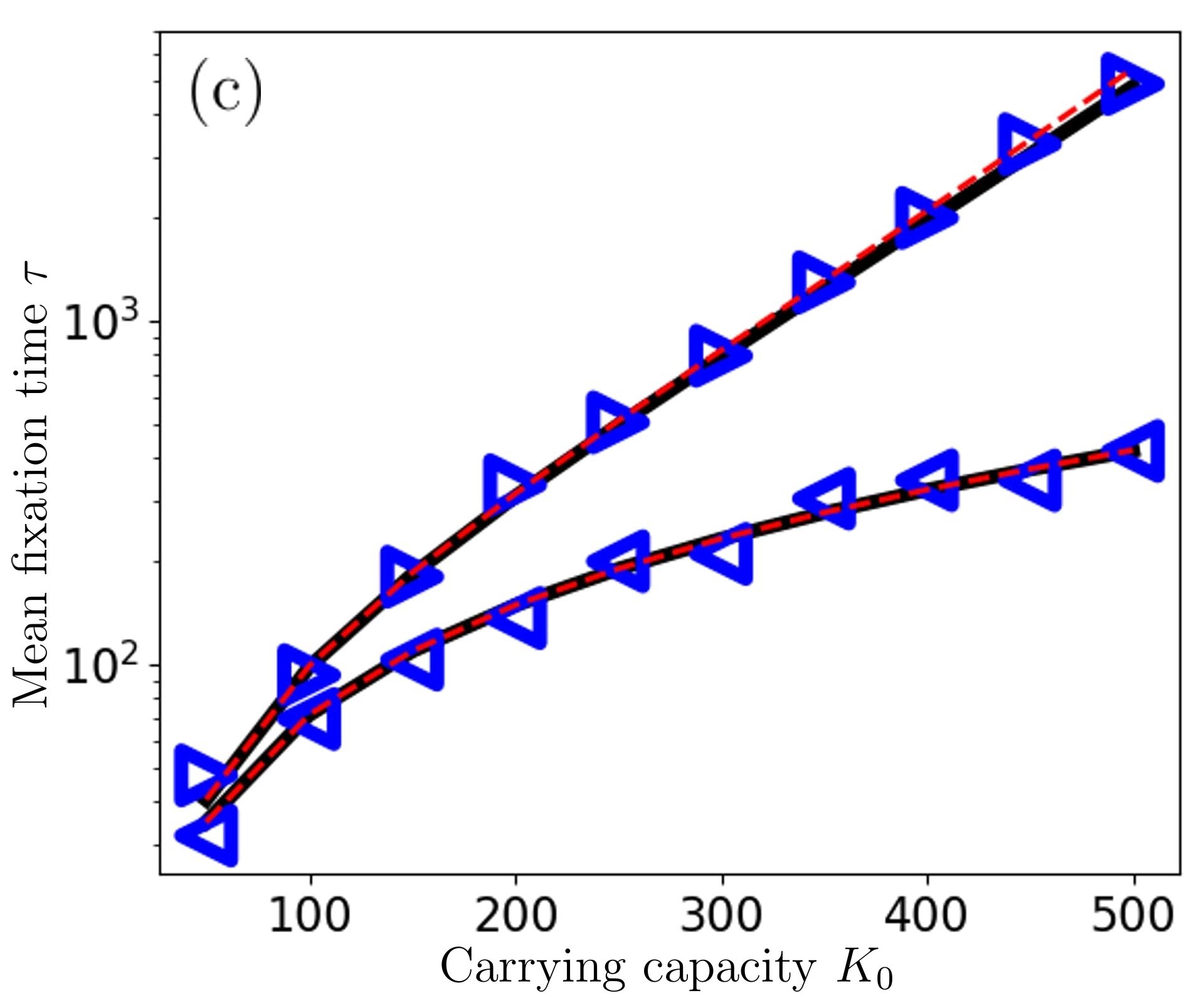
see Sec. SM3.A the appendix. A similar analysis can also be carried out for $\tau$, see Sec. SM3.B the appendix. Results reported in Fig. 2 show that Eqs. (III.2) and (14) accurately capture the behaviour of $\phi$ in the limiting regimes $\nu_{T}\to 0,\infty$, see Fig. 2(a). Fig. 2(b) shows that the predictions for $\tau$ when $\nu_{T}\to 0,\infty$, are also in good agreement with simulation results, with a much larger MFT under high $\nu_{T}$ than under low switching rate (at fixed $\delta_{T}$). In Fig. 2(b), the MFT when $\nu_{T}\gg 1$ for $\delta_{T}=0$ is significantly larger than under $\delta_{T}\neq 0$. This stems from $x^{*}=x_{0}=1/2$ being the attractor of Eq. (11) when $\delta_{T}=0$, but not being an equilibrium when $\delta_{T}=0.3$ or $\delta_{T}=0.5$. Fig. 2(a,b) also illustrate the excellent agreement between the predictions of the MA with $N=K_{0}$ and those obtained from stochastic simulations with $K=K_{0}$ constant. Note that typical error bars are shown for $\delta_{T}=0$ in Fig. 2(b). These are found to be small and almost coincide with the markers. For the sake of readability, we have thus omitted similar error bars from the other panels and figures.

The MF analysis and results of Fig. 2 suggest that under sufficiently high switching rate $\nu_{T}$ there is long-lived coexistence of the strains. We can rationalise this picture by noting that in the regime of dominance of one strain the MFT scales sublinearly with the population size $N$, while the MFT grows superlinearly (exponentially when $N=K_{0}\gg 1$, see Fig. 2(c)) in the regime of long-lived coexistence [101, 109, 110, 82]. The dominance and long-lived coexistence scenarios are separated by a regime where the MFT scales with the population size, i.e. $\tau\sim N$, where the dynamics is governed by random fluctuations. This leads us to consider that long-lived coexistence of the $R$ and $S$ strains arises whenever the MFT exceeds $2\langle N\rangle$, i.e. when $\tau>2\langle N\rangle$, where $\langle N\rangle$ is the mean population size at (quasi-)stationarity; see below. This is illustrated in the provided videos of [111] commented in Sec. SM7 of the appendix. When, as in this section, $N=K_{0}$ or $N$ fluctuates about the constant carrying capacity $K_{0}$ ($N\approx K_{0}$), we simply have $\langle N\rangle=K_{0}$. The criterion $\tau>2\langle N\rangle=2K_{0}$ thus prescribes that long-lived coexistence occurs when the MFT scales superlinearly with $K_{0}$ and hence exceeds the double of the average population size, $2K_{0}\gg 1$.

Figure 3: Fixation/coexistence diagrams under $T$-EV in the $(\nu_{T},\delta_{T})$ parameter space for a small system of constant carrying capacity $K_{0}=50$, with selection bias $s=0.1$ (a,d), $s=1$ (b,e), and $s=10$ (c,f), after a time $t=2K_{0}$. (a)-(c): phase diagrams obtained from stochastic simulations of the model with a constant $K_{0}$ ($N$ fluctuates about $K_{0}$) over $10^{3}$ realisations and coded according to the RGB colourmap of panel (g): red / blue (grey / charcoal) corresponds to the likely fixation of $S/R$ (red (grey): $S$ dominance; blue (charcoal): $R$ dominance), regions indicated as “$S/R$ fixation” in panel (a); magenta (dark grey) indicates where fixation of $R$ or $S$ is likely, area between “$S/R$ fixation” regions in panel (a); green (light grey) indicates where long-lived coexistence is most likely, area highlighted as “$S+R$ coex.” in panel (c). (d)-(f): same as in (a)-(c) but from numerically exact solutions of Eq. (17) for the corresponding Moran process with a constant population size $N=K_{0}$, see text.

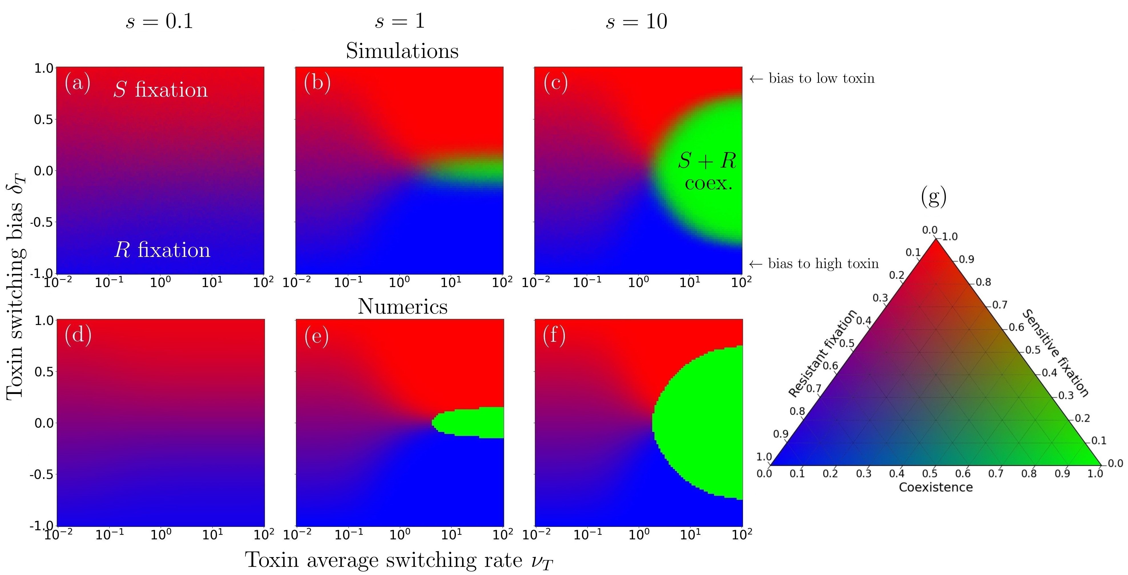
The conditions under which the long-lived coexistence criterion, $\tau>2\langle N\rangle$, is satisfied can be estimated by noting that, from the MF analysis, we expect coexistence to occur when $\xi_{T}$ self-averages under sufficiently high switching rate $\nu_{T}$. Since the average number of $T$-switches by $t=2\langle N\rangle$ scales as $\nu_{T}\langle N\rangle$, self-averaging occurs when $\nu_{T}\langle N\rangle\gg 1$. We thus consider that there is fast $T$-EV switching when $\nu_{T}\gg 1/\langle N\rangle$, while $\nu_{T}\ll 1/\langle N\rangle$ corresponds to the slow $T$-EV regime. To ensure long-lived coexistence, the necessary condition $\nu_{T}\gg 1/\langle N\rangle$ is supplemented by the requirement that $s\sim 1$. This ensures enough environmental variability and a regime of coexistence where the MFT is generally $\tau\sim e^{c\langle N\rangle}$ (where $c$ is some positive constant) when $s={\cal O}(1)$ [101, 109, 41, 42, 107, 108, 112] guaranteeing $\tau>2\langle N\rangle$.

Hence, the expected conditions for long-lived coexistence are $\nu_{T}\gg 1/\langle N\rangle$ (fast $T$-switching) and $s={\cal O}(1)$ (enough EV), which are satisfied in the examples considered here when $\nu_{T}\sim 1,s\sim 1$ or greater, and $\left\langle N\right\rangle\gg 1$.

We have studied the influence of $T$-EV on the fixation and coexistence properties of the model with constant carrying capacity $K=K_{0}$ and selection strength $s$ by running a large number of computer simulations up to a time $t=2K_{0}$ across the $\nu_{T}-\delta_{T}$ parameter space. When just after $t=2K_{0}$ both species are present, the run for $(\nu_{T},\delta_{T},s)$ is characterised by long-lived coexistence which is RGB coded $(0,1,0)$. There is no long-lived coexistence for the run $(\nu_{T},\delta_{T})$ if one of the species fixates by $t\leq 2K_{0}$: either the strain $R$, which is RGB coded $(1,0,0)$, or the strain $S$, which is coded by $(0,0,1)$. This procedure is repeated for $10^{3}$ realisations for different $(\nu_{T},\delta_{T})$ and, after sample averaging, yields the RGB-diagram of Fig. 3(a-c); see Sec. SM4 the appendix. In greyscale, the RGB coding translates into red $\rightarrow$ grey, blue $\rightarrow$ charcoal, and green $\rightarrow$ light grey. In what follows, the crossover regimes are coded in magenta and faint green with dark grey and faint light grey as their respective greyscale counterparts, see below.

It is also useful to study the effect of the $T$-EV in the realm of the MA by means of numerically exact results. For this, with the transition rates Eq. (7), we notice that when $N=K_{0}$ is constant and there are initially $n$ cells of type $R$, the $R$-strain fixation probability, $\phi_{n}^{\xi_{T}}$, in the environmental state $\xi_{T}$ satisfies the first-step analysis equation [98, 100, 53]

$$(\widetilde{T}_{R}^{+}(n)+\widetilde{T}_{R}^{-}(n)+\nu_{T}^{\xi_{T}})\phi_{n}^{\xi_{T}}=\leavevmode\nobreak\ \widetilde{T}_{R}^{+}(n)\phi_{n+1}^{\xi_{T}}+\widetilde{T}_{R}^{-}\phi_{n-1}^{\xi_{T}}$$

$$+\nu_{T}^{\xi_{T}}\phi_{n}^{-{\xi_{T}}},$$ (15)

subject to the boundary conditions $\phi_{0}^{\xi_{T}}=0$ and $\phi_{N}^{\xi_{T}}=1$. The mean fixation time in the environmental state $\xi_{T}$, $\tau_{n}^{\xi_{T}}$, satisfies a similar equation:

$$(\widetilde{T}_{R}^{+}(n)+\widetilde{T}_{R}^{-}(n)+\nu_{T}^{\xi_{T}})\tau_{n}^{\xi_{T}}=\leavevmode\nobreak\ 1+\widetilde{T}_{R}^{+}(n)\tau_{n+1}^{\xi_{T}}+\widetilde{T}_{R}^{-}(n)\tau_{n-1}^{\xi_{T}}$$

$$+\nu_{T}^{\xi_{T}}\tau_{n}^{-{\xi_{T}}},$$ (16)

with boundary conditions $\tau_{0}^{\xi_{T}}=\tau_{N}^{\xi_{T}}=0$. Eqs. (III.2) and (III.2) are thus solved numerically, and the fixation probability and MFT are obtained after averaging over the stationary distribution of $\xi_{T}$, yielding

$$\phi_{n} =\left(\frac{1+\delta_{T}}{2}\right)\phi_{n}^{+}+\left(\frac{1-\delta_{T}}{2}\right)\phi_{n}^{-},\quad\text{and}$$ (17)

$$\tau_{n} =\left(\frac{1+\delta_{T}}{2}\right)\tau_{n}^{+}+\left(\frac{1-\delta_{T}}{2}\right)\tau_{n}^{-}.$$

In our examples, we always consider $x_{0}=1/2$, and henceforth write $\phi_{{\rm MA}}(N)\equiv\phi_{N/2}$ for the $R$-fixation probability and $\tau_{{\rm MA}}(N)\equiv\tau_{N/2}$ for the MFT in the realm of the MA. For each triple $(\nu_{T},\delta_{T},s)$, we numerically solved Eq. (III.2) and, in the region of the the parameter space where $\tau_{{\rm MA}}(N)>2K_{0}$, there is long-lived coexistence, which is coded by $(0,1,0)$ in the RGB-diagram of Fig. 3(d-f). When $\tau_{{\rm MA}}(N)\leq 2K_{0}$, there is dominance of one of the species, characterised by the fixation probabilities $\phi_{{\rm MA}}(N)$ and $1-\phi_{{\rm MA}}(N)$ of $R$ and $S$, respectively, obtained from Eq. (III.2) and coded by $(\phi_{{\rm MA}}(N),0,1-\phi_{{\rm MA}}(N))$ in Fig. 3(d-f).

Exact numerical results for the MA with $N=K_{0}$ in Fig. 3(d-f) are in excellent agreement with those of simulations obtained for $K=K_{0}$ in Fig. 3(a-c). In line with the MF analysis, we find that long-lived coexistence, occurs for $T$-EV of sufficiently large magnitude, i.e. $s\sim 1$ or higher, and under high enough switching rate, i.e. $\nu_{T}\sim 1$ or higher, shown as green (light grey) areas in Fig. 3. The region of coexistence separates regimes dominated by either species, especially at high $\nu_{T}$ when $\phi\approx 0$ when $\delta_{T}\>0$ while $\phi\approx 1$ when $\delta_{T}<0$. In Fig. 3, the boundaries between the regimes of $R/S$ dominance, coded in blue (charcoal) / red (grey), and coexistence, areas in green (light grey)), are interspersed by crossover regimes where both species are likely to fixate (magenta (dark grey) in Fig. 3), or coexist with probability between 0 and 1 (faint green (faint light grey) in Fig. 3), as coded in Fig. 3(g).

IV Twofold Environmental Variability: Coexistence and fixation under time-varying fitness and switching carrying capacity

We have seen that under a constant carrying capacity, long-lived coexistence of the strains is feasible when $s$ and $\nu_{T}$ are of order $1$ or higher (enough $T$-EV and fast $T$-switching). We now study how this picture morphs when, in addition to the time-variation of $f_{S}$ and $\overline{f}$, the carrying capacity $K(t)$ switches according to Eq. (1) and drives the fluctuating population size $N$. EV is thus twofold, and the population evolves under the joint effect of $T$-EV and $K$-EV.

We consider $K(t)\in\{K_{-},K_{+}\}$ with $1\ll K_{-}<K_{+}$, and in the first instance assume that $N$ is always sufficiently large to allow us to neglect the DN, yielding [105, 57, 61, 62, 63, 66, 98]

$$\dot{N}=T_{R}^{+}-T_{R}^{-}+T_{S}^{+}-T_{S}^{-}=N\left(1-\frac{N}{K}\right),$$ (18a)

$$\dot{x}=\frac{T_{R}^{+}-T_{R}^{-}}{N}-x\frac{\dot{N}}{N}=x\left(\frac{f_{R}}{\overline{f}}-1\right),$$ (18b)

where $N$ is independent of $s$ and affected only by $K$-EV via ${\xi_{K}}$ in Eq. (1), while the evolution of $x$ in Eq. (18b) is impacted by $\xi_{K}$, $\xi_{T}$, and $s$ via $x=N_{R}/N$ and $\overline{f}(t)=x+(1-x)\exp(s\xi_{T}$). The population composition is hence coupled to the evolution of the population size (eco-evolutionary dynamics), while the statistics of $N$, like its average, denoted by $\langle N\rangle$, are obtained by ensemble averaging over $\xi_{K}$. The stochastic logistic differential equation Eq. (18a) defines an $N$-PDMP whose properties allow us to characterise the distribution of $N$ [105, 56, 57, 61].

Figure 4: Long-time average population size $\langle N\rangle$ versus the $K$-EV average switching rate $\nu_{K}$. Symbols are from simulations (averaged over $10^{3}$ realisations at time $t=2\langle K\rangle$), the solid black line shows the PDMP prediction Eq. (20). For fixed $\delta_{K}$, $\langle N\rangle$ decreases with $\nu_{K}$, and $\langle N\rangle\approx\langle K\rangle=K_{0}(1+\gamma\delta_{K})$ when $\nu_{K}\ll 1$ while $\langle N\rangle\approx\mathcal{K}$ when $\nu_{K}\gg 1$ (red horizontal dashed lines). Insets show the PDMP PDF Eq. (19) under low switching rate $\nu_{K}$ (left) and for $\nu_{K}\gg 1$ (right); dashed vertical lines are eye-guides indicating the corresponding values of $\nu_{K}$, where for low $\nu_{K}$ the PDMP PDF is indistinguishable in either case. Parameters are: $K_{0}=1000$, $\gamma=0.5$, and $\delta_{K}=0.0$. See text for details.

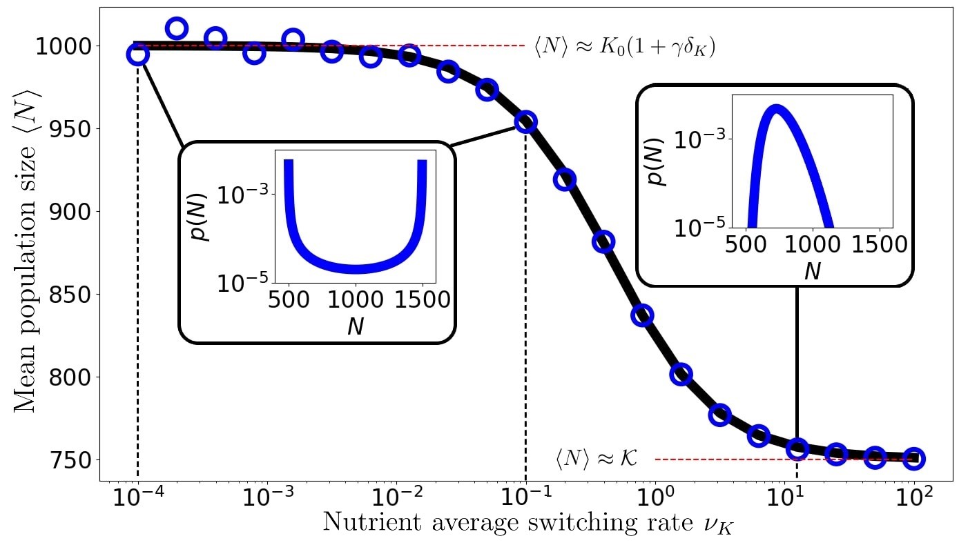
As discussed in [57, 61, 62, 63], the (marginal) stationary probability density function (PDF) $p(N)$ of the $N$-PDMP Eq. (18a), while ignoring DN, provides a useful approximation of the actual quasi-stationary population size distribution (QPSD). Here, the stationary PDF is [95, 96, 97, 57, 61, 62, 63]

$$p(N)=\frac{\mathcal{Z}}{N^{2}}\left(\frac{K_{+}-N}{N}\right)^{\nu_{K}(1-\delta_{K})-1}\left(\frac{N-K_{-}}{N}\right)^{\nu_{K}(1+\delta_{K})-1},$$ (19)

of support $[K_{-},K_{+}]$, with the normalisation constant $\mathcal{Z}$ ensuring that $\int_{K_{-}}^{K_{+}}p(N)\leavevmode\nobreak\ dN=1$.

IV.1 $N$-PDMP approximation

The PDF $p(N)$ captures well the main effects of the $K$-EV on the QPSD, which is bimodal under low $\nu_{K}$ and becomes unimodal when $\nu_{K}\gg 1$, see Fig. 4. In the realm of the $N$-PDMP approximation, $p(N)$ aptly reproduces the location of the QPSD peaks and the transition from a bimodal to unimodal distribution as $\nu_{K}$ increases: The distribution is sharply peaked around $N\approx K_{\pm}$ when $\nu_{K}\to 0$ (with probability $(1\mp\delta_{K})/2$), flattens when $\nu_{K}\sim 1$, and then sharpens about $N\approx\mathcal{K}\equiv K_{0}(1-\gamma^{2})/(1-\gamma\delta_{K})$ when $\nu_{K}\to\infty$. Since $p(N)$ ignores DN, it cannot capture the width of the QPSD about the peaks, but it provides an accurate description of the mean population size, see Fig. 4, that is well approximated by

$$\left\langle N\right\rangle=\int_{K_{-}}^{K_{+}}Np(N)\leavevmode\nobreak\ \text{d}N,$$ (20)

with $\langle N\rangle\approx K_{0}(1+\gamma\delta_{K})$ when $\nu_{K}\ll 1$ and $\langle N\rangle\approx\mathcal{K}$ when $\nu_{K}\gg 1$ [57, 61, 62, 63], as shown in Fig. 4.

The PDF $p(N)$ is particularly useful to obtain the fixation/coexistence diagrams under the effects of both $T$-EV and $K$-EV. Theoretical/numerical predictions of the fixation and coexistence probabilities can indeed be derived in the vein of [57, 61, 62, 63, 66] by focusing on situations where coexistence occurs when $x$ and $N$ relax on similar timescales. Long-lived coexistence of the strains thus arises when $s\sim 1$, with fixation typically occurring after $N$ has settled in the QPSD, see Sec. SM7 the appendix and videos in [111]. Hence, for the analytial description of the fixation/coexistence diagrams the $R$ fixation probability (with $x_{0}=1/2$) can be suitably approximated by averaging $\phi_{{\rm MA}}(N)$ over $p(N)$ as follows:

$$\phi\simeq\int_{K_{-}}^{K_{+}}\phi_{{\rm MA}}(N)p(N)\leavevmode\nobreak\ \text{d}N,$$ (21)

where $\phi_{{\rm MA}}(N)$ is obtained from solving the corresponding Eq. (III.2) for the $R$ fixation probability of the associated Moran process, as seen in Sec. III.2.

We can use the PDF $p(N)$ and the results for the mean fixation time $\tau_{{\rm MA}}(N)$, obtained from solving Eq. (III.2), to determine the probability of coexistence in the realm of the $N$-PDMP approximation. For this, we first solve Eq.(III.2) for $\tau_{{\rm MA}}(N^{*})=2\langle N\rangle$, where $\langle N\rangle$ is given by Eq. (20). Since $\tau_{{\rm MA}}$ is an increasing function of $N$, see Fig. 2(c), we have $\tau_{{\rm MA}}(N)>2\langle N\rangle$ for all $N>N^{*}$, which is the long-lived coexistence condition. Within the $N$-PDMP approximation, the lowest possible value of $N^{*}$ is $K_{-}$ (since $N\in[K_{-},K_{+}]$). We then determine the probability $\eta$ that this condition is satisfied by integrating $p(N)$ over $[{\rm max}(N^{*},K_{-}),K_{+}]$:

$$\eta\equiv\text{Prob.}\left\{\tau_{{\rm MA}}(N)>2\left\langle N\right\rangle\right\}=\int_{{\rm max}(N^{*},K_{-})}^{K_{+}}p(N)\leavevmode\nobreak\ \text{d}N,$$ (22)

where $N^{*}$ depends on both $T$-EV and $K$-EV (via $\left\langle N\right\rangle$), while the integrand depends only on $K$-EV. Clearly, $\eta\to 1$ when $N^{*}\to K_{-}$. Hence, long-lived coexistence is almost certain when $N^{*}\approx K_{-}$, i.e. whenever the mean-fixation time of the population of fixed size $N=K_{-}$ exceeds $2\left\langle N\right\rangle$. Based on the results of Sec. III.2, $\eta$ increases with $\nu_{T}$ and $s$, and thus for sufficiently large $\nu_{T}$ and $s$ (but not too large $\delta_{T}$), we expect $N^{*}\to K_{-}$ and $\eta\to 1$.

IV.2 Fixation/coexistence diagrams under $T$-EV and $K$-EV

Figure 5: Fixation/coexistence diagrams under $T$-EV and $K$-EV in the $(\nu_{T},\delta_{T})$ parameter space showing the influence of K-switching rate $\nu_{K}$ on the fixation and coexistence probabilities, for $\nu_{K}=5\times 10^{-6}$ (a,d), $\nu_{K}=5\times 10^{-3}$ (b,e), and $\nu_{K}=5$ (c,f). Other parameters are $K_{0}=1200$, $s=0.5$, $\gamma=2/3$, $\delta_{K}=0$. (a)-(c): phase diagrams obtained from stochastic simulations data collected at $t=2\langle N\rangle$ over $10^{3}$ realisations. (d)-(f): same as in (a)-(c) but from the theoretical predictions based on Eqs. (21) and (22), see text for details. All diagrams are colour-coded (greyscale-coded) as in Fig. 3.

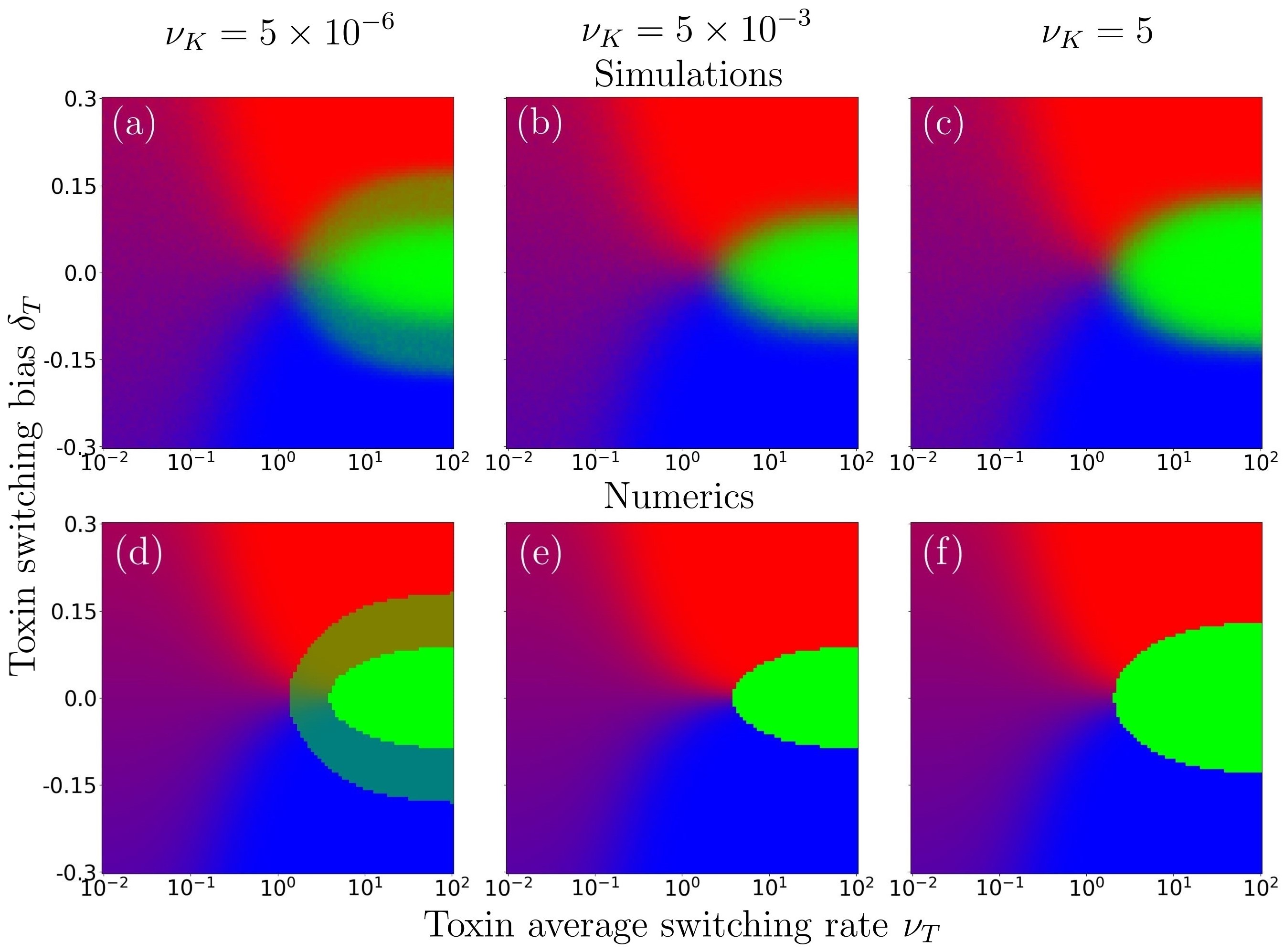
The fixation/coexistence diagrams under joint effect of $T$-EV and $K$-EV are obtained as in Sec. III.2, with the difference that long-lived coexistence arises when $t>2\left\langle N\right\rangle$, a condition that depends on $(\nu_{K},\delta_{K})$, see Fig. 2(c). In our simulations, we considered different values of $\nu_{K}$ (letting $\delta_{K}=0$ for simplicity), and ran simulations until $t=2\left\langle N\right\rangle$. Each run in which both species still coexist just after $t=2\left\langle N\right\rangle$ are RGB (greyscale) coded $(0,1,0)$, whereas those in which $R$ or $S$ fixates by $t\leq 2\left\langle N\right\rangle$ are respectively RGB (greyscale) coded $(1,0,0)$ or $(0,0,1)$. The RGB (greyscale) fixation/coexistence diagrams of Fig. 5(a-c) are obtained after sample-averaging the outcome of this procedure, repeated $10^{3}$ times for each pair $(\nu_{T},\delta_{T})$ and different values of $\nu_{K}$.

Theoretical RGB (greyscale) diagrams are obtained from the $N$-PDMP based approximation built on Eqs. (21) and (22): for a given $\nu_{K}$, we allocate the RGB (greyscale) value $((1-\eta)(1-\phi),\eta,(1-\eta)\phi)$ obtained for each pair $(\nu_{T},\delta_{T})$ of the diagram, see Fig. 5(d-f). This triple corresponds to the probability of having, by $t=2\left\langle N\right\rangle$, either no long-lived coexistence (with probability $1-\eta$) and fixation of $R$ or $S$ (with respective probabilities $\phi$ and $1-\phi$), or long-lived coexistence (with probability $\eta$). In practice, Eqs. (21) and (22) have been used for relatively small systems whereas an equivalent, but more efficient, method was used for large systems, see Sec. SM4 the appendix.

The comparison of the top and bottom rows of Fig. 5 shows that the theoretical RGB (greyscale) diagrams quantitatively reproduce the features of those obtained from simulations. In general, we find that coexistence regions are brighter in diagrams obtained from $N$-PDMP based approximation than in those stemming from simulations. This difference stems from former ignoring demographic fluctuations which slightly broaden the crossover (magenta (dark grey) and faint green (faint light grey)) regimes in the latter.

The regions of Fig. 5 where $|\delta_{T}|\to 1$ are characterised by dominance of one of the strains, and essentially reduces to the model studied in [57, 61, 63], and we can therefore focus on characterising the coexistence phase.

When $K_{0}$ is large, under sufficient environmental variability ($s=0.5$, $\gamma=2/3$ in Fig. 5), the joint effect of $T$-EV and $K$-EV on the phase of long-lived coexistence in the RGB (greyscale) diagrams of Fig. 5 can be summarised as follows: (i) when $\nu_{K}\to 0$, a (bright green) region where $\eta\approx 1$ and coexistence is almost certain is surrounded by a faint green (faint light grey)“outer shell” where coexistence is possible but not certain ($0<\eta<1$), see Fig. 5(a,d); (ii) at low, but non-vanishingly small, values of $\nu_{K}$, the outer-shell where $0<\eta<1$ fades, and there is essentially only a bright green (bright light grey) region of coexistence where $\eta\approx 1$, see Fig. 5(b,e); (iii) when $\nu_{K}\gg 1$, the coexistence region corresponds essentially to $\eta\approx 1$ (bright green / bright light grey) and is broader than under low $\nu_{K}$, Fig. 5(c,f). In all scenarios (i)-(iii), $\eta$ increases with $\nu_{T}\gtrsim 1$ (for not too large $\delta_{T}$) and hence all the green (bright and faint light grey) coexistence phases in Fig. 5) become brighter as $\nu_{T}$ is raised and $\eta\to 1$.

These different scenarios can be explained by the dependence of the QPSD on $\nu_{K}$, well captured by the PDF Eq. (19). In regime (i) where $\nu_{K}\ll 1/K_{0}$, the QPSD and $p(N)$ are bimodal, $N\approx K_{\pm}$ with probability $(1\pm\delta_{K})/2$, and any $K$-switches by $t=2\left\langle N\right\rangle\sim K_{0}$ are unlikely, yielding the faint green (faint light grey) outer shell of Fig. 5(a,d) corresponding to long-lived coexistence arising only when $N\approx K_{+}$, with a probability $\eta\approx(1+\delta_{K})/2$. In regime (ii), where $1/K_{0}\ll\nu_{K}\ll 1$, the QPSD and $p(N)$ are still bimodal but some $K$-switches occur by $t\sim K_{0}$, resulting in long-lived coexistence arising almost only when $\nu_{T}$ is high enough to ensure $\eta\approx 1$ when $N\approx K_{-}$. In regime (iii), where $\nu_{K}\gg 1$ the QPSD and $p(N)$ are unimodal with average $\left\langle N\right\rangle\approx{\cal K}\geq K_{-}$, which results in a long-lived coexistence region where $\eta\approx 1$ that is broader than in (i) and (ii), Fig. 5(c,f). The size of the coexistence region in regime (iii) actually depends nontrivially on $\nu_{K}$, as revealed by the modal value of the PDF Eq. (19) when $\nu_{K}(1-|\delta_{K}|)>1$, which reads

$$\hat{N}=\leavevmode\nobreak \frac{K_{0}}{2}\left[1+\nu_{K}(1-\gamma\delta_{K})\right]$$ (23)

$$-\frac{K_{0}}{2}\sqrt{(1+\nu_{K}(1-\gamma\delta_{K}))^{2}-4\nu_{K}(1-\gamma^{2})},$$

with $\lim_{\nu_{K}\to\infty}\hat{N}=\left\langle N\right\rangle=\mathcal{K}$. We notice that $\hat{N}$ is an increasing function of $\nu_{K}$ when $\gamma>\delta_{K}$, and it decreases if $\gamma<\delta_{K}$ (remaining constant when $\gamma=\delta_{K}$). As a consequence, the long-lived coexistence region under high $K$ switching rate grows with $\nu_{K}$ when $\gamma>\delta_{K}$, as in Fig. 5(c,f), and, when $\gamma<\delta_{K}$, shrinks as $\nu_{K}$ is increased, see Sec. SM6 Fig. (S3) the appendix.

IV.3 Influence of the $K$-EV amplitude on coexistence

Figure 6: Fixation/coexistence diagrams under $T$-EV and $K$-EV in the $(\nu_{T},\delta_{T})$ parameter space showing the effect of the amplitude of $K$-EV $\gamma$ on the fixation and coexistence probabilities when $K_{0}=500$ is kept fixed, for $\gamma=0.65$ $\left(K_{-}=175,\right.$ $\left.K_{+}=825\right)$ (a,d), $\gamma=0.8$ $\left(K_{-}=100,\right.$ $\left.K_{+}=900\right)$ (b,e), and $\gamma=0.95$ $\left(K_{-}=25,\right.$ $\left.K_{+}=975\right)$ (c,f). Other parameters are $s=1.0$, $\delta_{K}=0$, $\nu_{K}=10^{-3}$ in (a)-(c) and $\nu_{K}=10$ in (d)-(f). Phase diagrams obtained from stochastic simulations data collected at $t=2\langle N\rangle$ over $10^{3}$ realisations. All diagrams are colour-coded (greyscale-coded) as in Fig. 3.

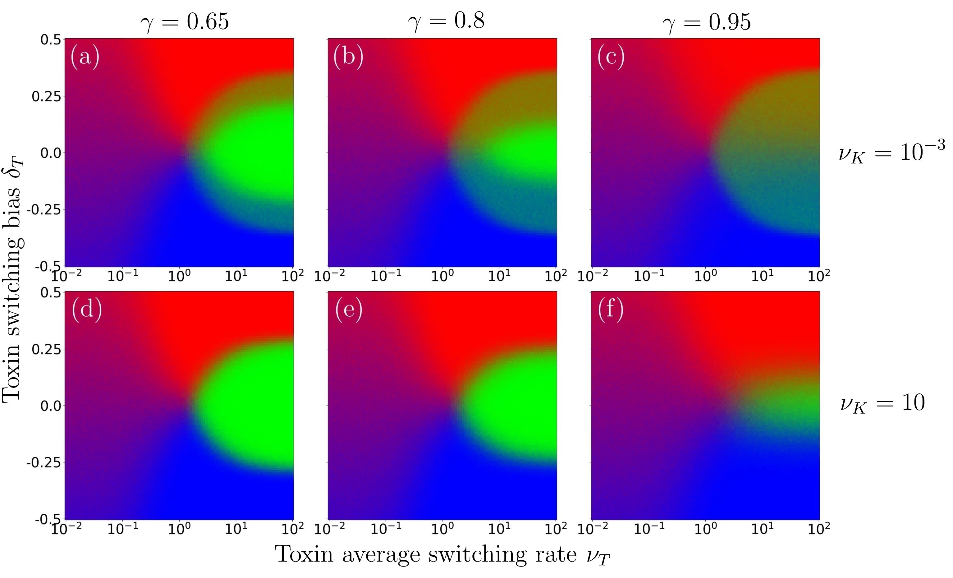
We have seen that increasing the selection bias $s$, raises the amplitude of the $T$-EV and facilitates the emergence of long-lived coexistence. Here, by keeping $K_{0}$ constant, we investigate the influence of the parameter $\gamma$, which controls the amplitude of $K$-EV, on the fixation/coexistence diagrams. When $\gamma\to 1$ and $K_{0}\gg 1$, there is $K$-EV of large amplitude, with the population subject to a harsh population bottleneck ($K_{-}\to 0$) accompanied by strong demographic fluctuations. The latter facilitate fixation of either strain and counter the effect of $T$-EV that drives the community to coexistence. Results of Fig. 6 illustrate the influence of $\gamma$ under low and high $K$-switching rate ($\delta_{K}=0$):

1. Under low $\nu_{K}$, the probability of long-lived coexistence $\eta$ decreases together with the value of $K_{-}=K_{0}(1-\gamma)$ when $\gamma$ is increased (all other parameters being kept fixed). As a consequence, the bright green (bright light grey) region in Fig. 6(a) where long-lived coexistence is almost certain ($\eta\approx 1$) shrinks with $\gamma$ and is gradually replaced by a faint green (faint light grey) area where coexistence occurs with a lower probability ($\eta=(1+\delta_{K})/2<1$), see Fig. 6(b,c).

2. Under high $\nu_{K}$, we have $N\approx\mathcal{K}$ and the effect of $\gamma$ is encoded in the expression of $\mathcal{K}=K_{0}(1-\gamma^{2})/(1-\gamma\delta_{K})$. When $\delta_{K}\leq 0$, $\mathcal{K}$ and $\eta$ decrease with $\gamma$, and as a result the bright green (bright light grey) region in Fig. 6(d) shrinks and is eventually replaced by a smaller faint green (faint light grey) region where coexistence is possible but not certain ($0<\eta<1$), see Fig. 6(e,f). When $\delta_{K}>0$, there is a bias towards $K=K_{+}$ and $\mathcal{K}$ increases with $\gamma$ until $\gamma=\bar{\gamma}\equiv(1-\sqrt{1-\delta_{K}^{2}})/\delta_{K}$ and then decreases, with $\mathcal{K}<K_{0}$, when $\gamma>\delta_{K}$. This results in a non-monotonic dependence of the coexistence region where $\eta\approx 1$: under $\nu_{K}\gg 1$ and $\delta_{K}>0$, the long-lived (bright-green) coexistence region grows with $\gamma$ up to $\bar{\gamma}$ and shrinks when $\gamma>\bar{\gamma}$.

We have thus found that the environmental fluctuations have opposite effects on the species coexistence: increasing the amplitude of $T$-EV (by raising $s$) prolongs the coexistence of the strains and expands the coexistence region, but raising the amplitude of $K$-EV (by raising $\gamma$) can significantly reduce the probability of long-lived coexistence for all values of $\nu_{K}$.

V Make-up of the coexistence phase and strains average abundance

Having characterised in detail the conditions under which long-lived coexistence and fixation occur, we now study the make-up of the coexistence phase and then use this result to determine the stationary average abundance of each strain.

V.1 Coexistence phase make-up

Figure 7: Make-up of the coexistence state: fraction of the resistant strain $R$ in the coexistence phase as function of $\nu_{T}$ and $\delta_{T}$; from simulation results (a) and predictions of Eqs. (12) and (22) in (b), respectively for $x^{*}$ and $\eta$. The colourbar (brightness bar) gives the characteristic fraction of the $R$ strain in the region of the $\nu_{T}$-$\delta_{T}$ parameter space where $\eta>0.01$. Simulation results have been obtained just after $t=2\langle N\rangle$ and averaged over $10^{4}$ realisations. Parameters are $K_{0}=500$, $\gamma=0.5$, $\nu_{K}=100$, and $s=1$.

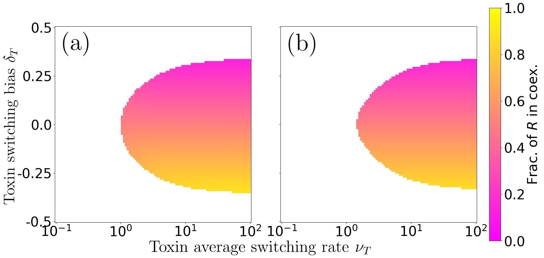
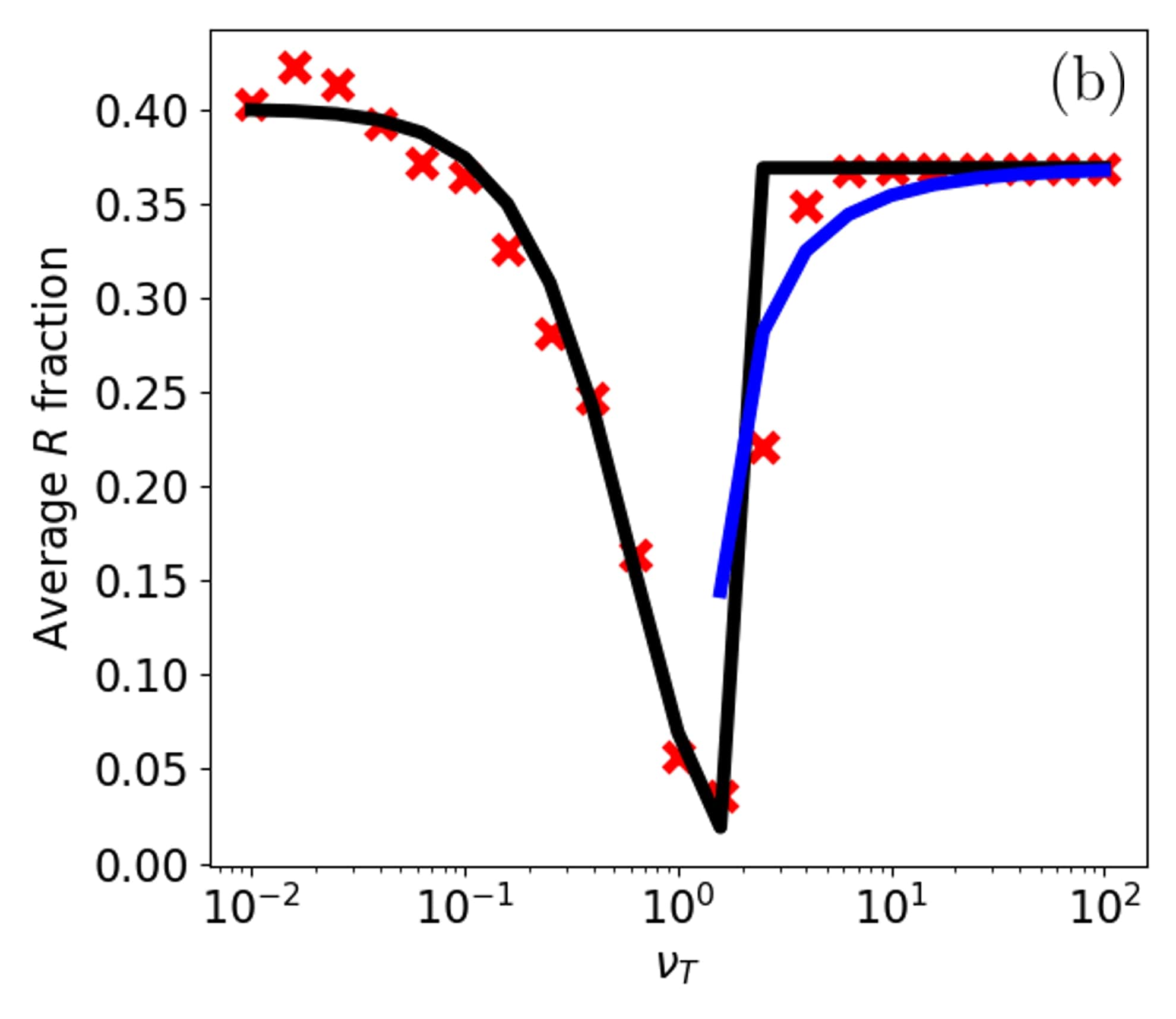
We are interested in the characteristic fraction of the resistant strain $R$ in the coexistence phase, here defined as $x^{*}$. This is the fraction of $R$ expected, given that we have coexistence at $t=2\left\langle N\right\rangle$. According to the mean-field theory, the fraction of the strain $R$ in the coexistence phase is given by the expression Eq. (12) of $x^{*}$. It turns out that deep into the coexistence region whereby $\eta\approx 1$ and $\nu_{T}$ is sufficiently high, there is good agreement between theory and simulations, see Fig. 7(a,b). In addition, even when $\eta<1$, the mean-field prediction $x^{*}$ remains remarkably close to the value of fraction of $R$ measured in the coexistence state obtained in simulations, with small deviations arising as $\eta$ approaches 0. We notice that the characteristic fraction of $R$, for given $\delta_{T}$, is almost independent of $\nu_{T}$.

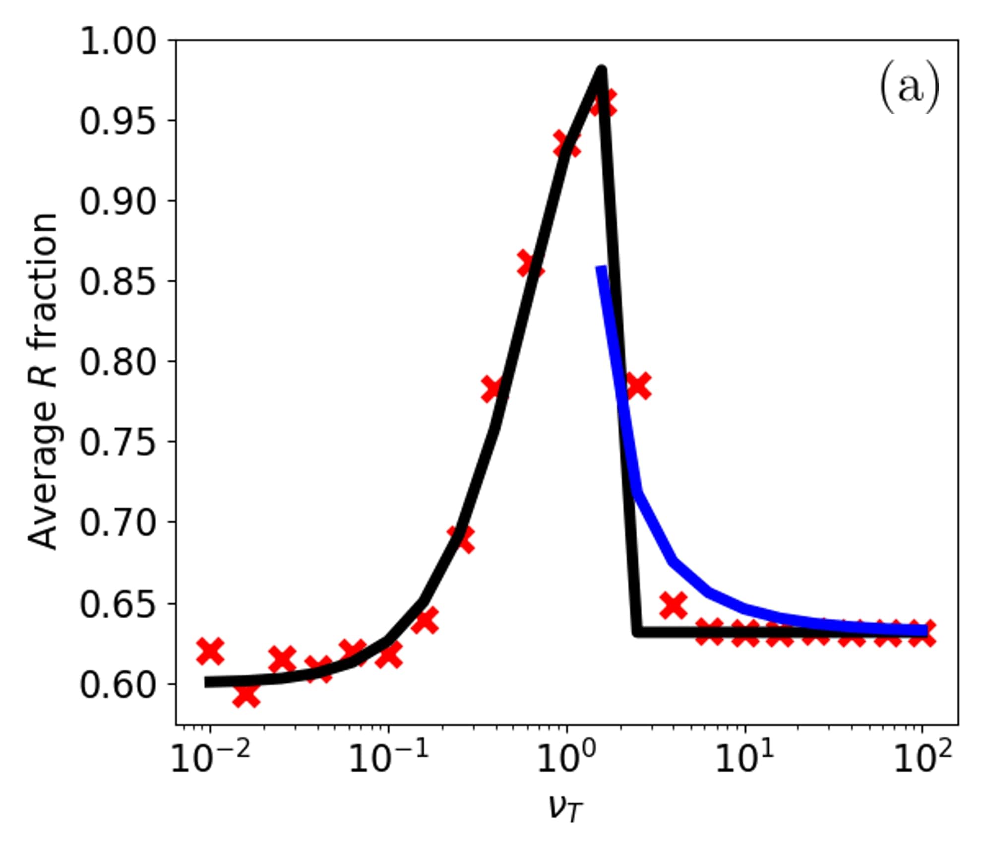
We can also predict the fraction of $R$ regardless of coexistence or fixation, here denoted by $\left\langle x\right\rangle$. The quantity $\left\langle x\right\rangle$ thus characterises the fraction of $R$ in the coexistence, fixation, and crossover regime where both coexistence and fixation are possible, with respective probabilities $\eta$ and $\phi$, but neither is certain. Making use of Eqs. (12), (21), and (22) we thus define $\left\langle x\right\rangle$ as

$$\left\langle x\right\rangle=\eta x^{*}+(1-\eta)\phi.$$ (24)

This captures well the dependence of $\left\langle x\right\rangle$ on $\nu_{T}$ and reduces to the fraction of $R$ in the coexistence phase, $\left\langle x\right\rangle=x^{*}$, when $\eta\approx 1$ and long-lived coexistence is almost certain (see SM5, Fig. S2). As shown in Sec. SM5 of the appendix, a closed-form alternative to $\left\langle x\right\rangle$ is provided by the modal value of the stationary PDF of the PDMP defined by Eq. (8), which, while less accurate than $\left\langle x\right\rangle$, matches qualitatively well to simulations.

V.2 Strain average abundance

Figure 8: Long-time average $R$ abundance $\langle N_{R}\rangle$ as function of the average switching rate of the $T/K$-EV. Solid lines are theoretical predictions of Eq. (25) with $x^{*}$, $\langle N\rangle$, $\phi$ and $\eta$ given by Eqs. (12), (20)-(22); symbols are from simulation data. (a) $\langle N_{R}\rangle$ versus $\nu_{K}$ for $\delta_{K}=0.5$ ($\mathbf{\times}$), $\delta_{K}=0$ ($\mathbf{\bigcirc}$) and $\delta_{K}=-0.5$ ($\mathbf{\bigtriangledown}$). Limiting value are plotted for $\nu_{K}\rightarrow 0,\infty$ as dotted lines. Other parameters are: $K_{0}=500$, $\gamma=0.5$, $s=1.0$, $\nu_{T}=10$, and $\delta_{T}=0.0$. (b) $\langle N_{R}\rangle$ versus $\nu_{T}$ for $(\delta_{T},\nu_{K})=(-0.2,0.01)$ ($\bigtriangleup$), $(\delta_{T},\nu_{K})=(-0.2,10)$ (

$\bigtriangleup$

),$(\delta_{T},\nu_{K})=(0.2,0.01)$ (

$\bigtriangleup$

), $(\delta_{T},\nu_{K})=(0.2,10)$ ($\lozenge$). Limiting value are plotted for $\nu_{T}\rightarrow 0,\infty$ as dotted lines. Other parameters are: $K_{0}=500$, $\gamma=0.5$, $s=1.0$, and $\delta_{K}=0.0$. Simulations data have been collected and sample-averaged after $t=2\langle K\rangle$ over $10^{2}$ realisations. See text for details.

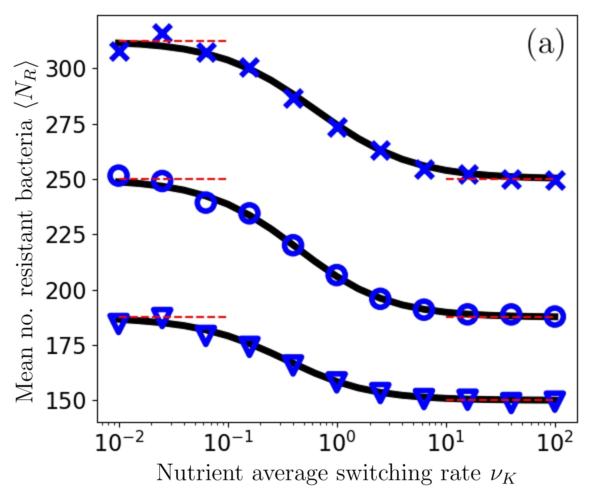
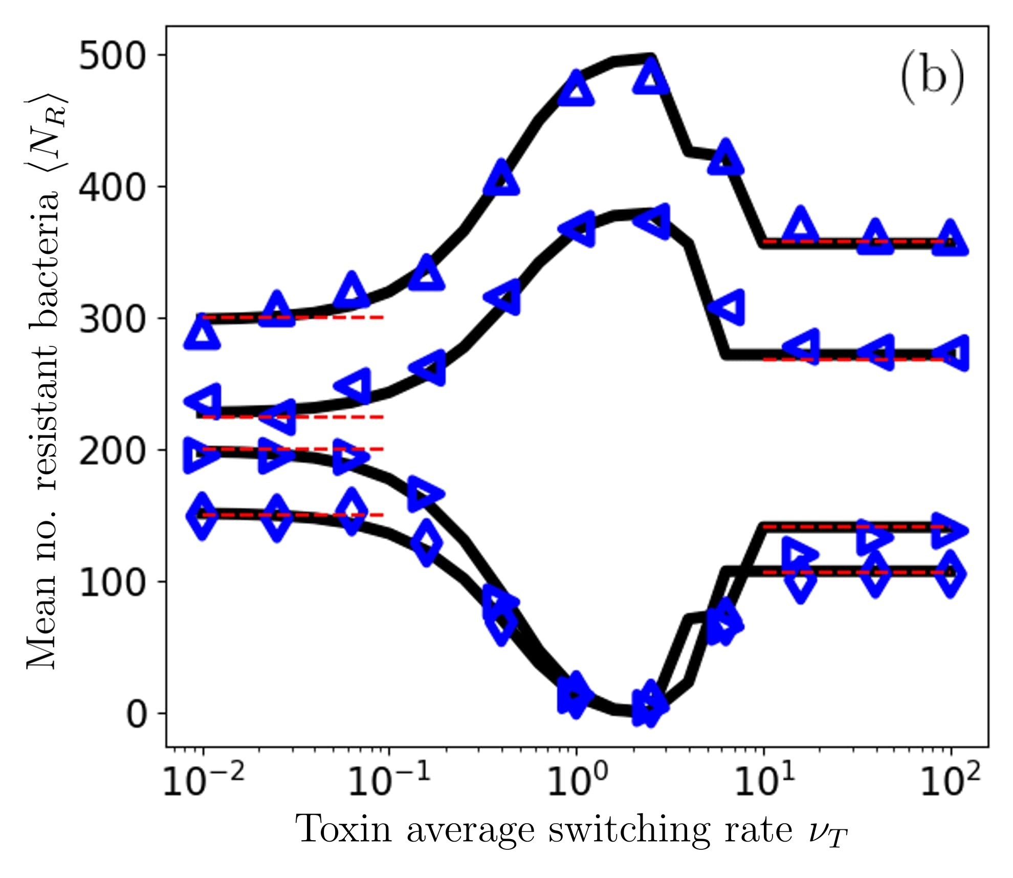
In this section, we study the (quasi-)stationary average abundance of the strains $R$ and $S$, respectively denoted by $\left\langle N_{R}\right\rangle$ and $\left\langle N_{S}\right\rangle$. Since $\left\langle N_{S}\right\rangle=\left\langle N\right\rangle-\left\langle N_{R}\right\rangle$, and $\left\langle N\right\rangle$ is well described by Eq. (20), see Fig. 4, we only need to focus on studying $\left\langle N_{R}\right\rangle$.

In fact, while the evolution of $N$ is governed by $K$-EV and is well-captured by the stochastic logistic equation Eq. (18a) and the corresponding $N$-PDMP, the dynamics of the abundance of the $R$ strain depends on both $T$-EV and $K$-EV. In the mean-field limit, where demographic fluctuations are neglected, we indeed have [98]

$$\dot{N}_{R}=T_{R}^{+}-T_{R}^{-} =\left(\frac{1}{\overline{f}(t)}-\frac{N}{K(t)}\right)N_{R}$$

$$=\left(\frac{1}{x+(1-x)e^{s\xi_{T}}}-\frac{N}{K_{0}(1+\gamma\xi_{K})}\right)N_{R},$$

which is a stochastic differential equation depending on both $\xi_{K}$ and $\xi_{T}$, and coupled to the $N$- and $x$-PDMPs defined respectively by Eqs. (18a) and (18b). In the dominance regimes, $\left\langle N_{R}\right\rangle\approx 0$ ($S$ dominance) or $\left\langle N_{R}\right\rangle\approx\left\langle N\right\rangle$ ($R$ dominance), which can be obtained from Eq. (20). However, finding $\left\langle N_{R}\right\rangle$ in the coexistence phase is a nontrivial task. Progress can be made by noticing that, $\xi_{K}$ and $\xi_{T}$ being independent, we can write

$$\left\langle N_{R}\right\rangle\approx\left\langle N\right\rangle\left\langle x\right\rangle\equiv\left\langle N\right\rangle(\eta x^{*}+(1-\eta)\phi),$$ (25)

where $\left\langle N\right\rangle\eta x^{*}$ is the contribution to $\left\langle N_{R}\right\rangle$ when there is coexistence (with probability $\eta$), and $\left\langle N\right\rangle(1-\eta)\phi$ is the contribution arising when there is fixation of the strain $R$ (with probability $(1-\eta)\phi$). In our theoretical analysis, $x^{*},\left\langle N\right\rangle,\phi$ and $\eta$ are obtained from Eqs. (12) and (20)-(22). Eq. (25) thus captures the behaviour of $\left\langle N_{R}\right\rangle$ in each regime: the dominance regime where $\eta\approx 0$ and we have $\left\langle N_{R}\right\rangle\approx\left\langle N\right\rangle\phi$, deep in the coexistence phase where we have $\eta\approx 1$ and $\left\langle N_{R}\right\rangle\approx\left\langle N\right\rangle x^{*}$, and where $0<\eta<1$ and coexistence is possible but not certain where we have $\left\langle N_{R}\right\rangle\approx\left\langle N\right\rangle\left\langle x\right\rangle$.

In Fig. 8, we find that the theoretical predictions based on Eq. (25) agree well with simulation results over a broad range of $\nu_{K}$ and $\nu_{T}$, and for different values of $\delta_{K}$ and $\delta_{T}$. The dependence of $\left\langle N_{R}\right\rangle$ on $\nu_{K}$ reflects that of $\left\langle N\right\rangle$ shown in Fig. 4: $\left\langle N_{R}\right\rangle$ decreases with $\nu_{K}$ at fixed $\delta_{K}$, see Fig. 8(a), and we have $\left\langle N\right\rangle\approx{\cal K}$ when $\nu_{K}\to\infty$ yielding $\left\langle N_{R}\right\rangle\approx{\cal K}x^{*}$ deep in the coexistence phase where $\nu_{T}\gg 1$, and similarly $\left\langle N\right\rangle\approx K_{0}(1+\gamma\delta_{K})$ when $\nu_{K}\to 0$ yields $\left\langle N_{R}\right\rangle\approx K_{0}(1+\gamma\delta_{K})x^{*}$. Not shown in Fig. 8(a) is the case of $\nu_{T}\ll 1$, whereby we have only dominance such that $\left\langle N_{R}\right\rangle\approx\left\langle N\right\rangle(1-\delta_{T})/2$. Fig. 8(b) shows that the dependence of $\left\langle N_{R}\right\rangle$ on $\nu_{T}$ can be non-monotonic and exhibit an extreme dip ($\delta_{T}>0$) or peak ($\delta_{T}<0$) at intermediate $T$-switching rate, $\nu_{T}\sim 1$. This behaviour can be understood by referring to the diagrams of Fig. 6: as $\nu_{T}$ is raised from $\nu_{T}=0$ with $\delta_{T}<0$ kept fixed, the $R$ fixation probability first slowly increases across the slightly $R$-dominant phase where coexistence is unlikely ($\eta\approx 0$) and $\left\langle N_{R}\right\rangle\approx\left\langle N\right\rangle\phi$. When $\nu_{T}$ is increased further and $R$ is the strongly dominant species (blue (charcoal) phases in Fig. 6), with $\phi\approx 1$ and $\left\langle N_{R}\right\rangle\approx\left\langle N\right\rangle$ is maximal; coexistence then becomes first possible ($0<\eta<1$, faint green (faint light gray) in Fig. 6) and then almost certain ($\eta\approx 1$, bright green (bright light gray) in Fig. 6) when $\nu_{T}$ is increased further, which results in a reduction of the $R$ abundance to $\left\langle N_{R}\right\rangle\approx\left\langle N\right\rangle x^{*}<\left\langle N\right\rangle$. A similar reasoning holds for the $S$ strain when $\delta_{T}>0$ and results in a maximal value $\left\langle N_{S}\right\rangle\approx\left\langle N\right\rangle$ and therefore a dip of the $R$ abundance, with a minimal value $\left\langle N_{R}\right\rangle\approx 0$, when $\nu_{T}\sim 1$.

The results of this section hence show that the twofold EV has nontrivial effects on the make-up of the coexistence phase, and on the average number of cells of each strain, as shown by Fig. 7 and the nonmonotonic dependence of $\left\langle N_{R}\right\rangle$ on $\nu_{T}$ in Fig. 8.

VI Conclusion

Microorganisms live in environments that unavoidably fluctuate between mild and harsh conditions. Environmental variability can cause endless changes in the concentration of toxins and amount of available nutrients, and thus shapes the eco-evolutionary properties of microbial communities including the ability of species to coexist. Understanding under which circumstances various microbial species can coexist, and how their coexistence and abundance vary with environmental factors, is crucial to shed further light on the mechanisms promoting biodiversity in ecosystems and to elucidate the evolution of antimicrobial resistance (AMR).

Motivated by these considerations, and inspired by the antimicrobial resistance evolution in a chemostat setup, we have studied the eco-evolutionary dynamics of an idealised microbial community of fluctuating size consisting of two strains competing for the same resources under twofold environmental variability ($T$-EV and $K$-EV): the level of toxin and the abundance of nutrients in the community both vary in time. One of the strains is resistant while the other is sensitive to the drug present in the community, and both compete for the same resources.

Environmental variability is thus assumed to affect the strains growth and death rates, and is modelled by means of binary randomly time-switching fitness ($T$-EV) and carrying capacity ($K$-EV). Under harsh conditions, the level of toxin is high and resources are scarce, while environmental conditions are mild when the level of toxin is low and resources are abundant. In this setting, the strain resistant to the drug has a selective advantage under high toxin-level, whereas it is outgrown by the sensitive strain when the level of toxin is low. Moreover, the time-switching carrying capacity drives the fluctuating size of the microbial community, which in turn modulates the amplitude of the demographic fluctuations, resulting in their coupling with the variation of the available resources. When the environment is static, there is no lasting coexistence since one species dominates and rapidly fixates the entire population.
Here, we have shown that this picture changes radically in fluctuating environments: we have indeed found that long-lived species coexistence is possible in the presence of environmental fluctuations. Using stochastic simulations and the properties of suitable piecewise-deterministic and Moran processes, we have computationally and analytically obtained the fixation-coexistence phase diagrams of the system. These have allowed us to identify the detailed environmental conditions under which species coexist almost certainly for extended period of times, and the phases where one species dominates, as well as the crossover regimes where both coexistence and fixation are possible but not guaranteed. We have found that long-lived coexistence requires sufficient variation of the toxin level, while resource variability can oppose coexistence when strong $K$-EV leads to population bottlenecks responsible for large demographic fluctuations facilitating fixation. More generally, our analysis has allowed us to assess the influence of the population size distribution, whose shape changes greatly with the rate of $K$-EV, on the fixation-coexistence phase diagram. We have also determined how the make-up of the coexistence phase and average abundance of each strain depend on the rates of environmental change.

Environmental variability generally comes about in many forms in a variety of settings throughout biology and ecology, and the conundrum of coexistence within a system is impacted by it, alongside demographic fluctuations. This leads to complex eco-evolutionary dynamics. In particular, how microbial communities evolve subject to environmental variability is vital when considering the issue of AMR, so that the effectiveness of treatments can be maximised, while minimising the harmful effects. In considering twofold environmental variations, we have shown that these can have qualitative effects on the population evolution as they can either promote or jeopardise lasting species coexistence.

In summary, our analysis allows us to understand under which circumstances environmental variability, together with demographic fluctuations, favours or hinders the long-lived coexistence of competing species, and how it affects the fraction and abundance of each strain in the community. This work hence contributes to further elucidate the role of fluctuations on the maintenance of biodiversity in complex ecosystems.

In particular, our findings demonstrate the influence of environmental fluctuations on biodiversity in microbial communities, and may thus have potential impacts on numerous applications. For instance, the model studied here is well suited to describe the in vitro evolution of antimicrobial resistance in a chemostat setup where the level of antibiotics would fluctuate below and above the minimum inhibitory concentration. In this context, the model is able to predict, under a broad range of external constraints, the best conditions to avoid the fixation of the strain resistant to the drug and when both strains coexist. A more realistic model of AMR evolution would take into account that the drug resistance is often mediated by a form of public goods [36, 79], and that there may exist more than two competing species and various toxins. The eco-evolutionary dynamics of communities consisting of multiple species, resources and toxins can generally not be simply inferred from those of two-species eco-systems, even though in some cases simple models can be illuminating [65]. Another potential application of the model considered here, with varying drug levels, concerns the so-called adaptive therapy used in cancer treatment to prevent or delay the cancer from becoming completely drug resistant [113].

Data accessibility

The data that support the findings of this study are openly available, see [114].

Author Contributions

Matthew Asker: Conceptualisation (supporting), Methodology, Formal Analysis (lead), Software, Writing - Original Draft, Writing - Review & Editing, Visualisation, Investigation, Validation.
Lluís Hernández-Navarro: Formal Analysis (supporting), Writing - Review & Editing (supporting), Supervision (supporting).
Alastair M. Rucklidge: Writing - Review & Editing (supporting), Supervision (supporting), Funding acquisition (supporting).
Mauro Mobilia: Conceptualisation (lead), Methodology (lead), Formal Analysis (supporting), Writing - Original Draft, Writing - Review & Editing, Visualisation, Supervision (lead), Project administration, Funding acquisition (lead).

Appendix

In this appendix, we provide some further technical details and supplementary information in support of the results discussed in the main text. We also provide additional information concerning the mean-field, Moran and PDMP approximations used in the main text, the simulation methods, we illustrate our main findings by discussing typical sample paths, and briefly discuss the generalisation of the model to correlated/anticorrelated EV.

SM1. Table of parameters and physical quantities of interest

The various parameters of the model and physical quantities of interest are summarised in the following table.

Table 1: Table of parameters and physical quantities of interest.

Parameter / Quantity	Notation / Definition
Population size	$N$
Population size of type $i\in\{R,S\}$	$N_{i}$
Population size of type $i\in\{R,S\}$	$f_{i}$
Selection strength / strength of toxin environmental variability	$s$
Dichotomous Markov Noise variable for noise of type $\alpha\in\{T,K\}$	$\xi_{\alpha}$
Carrying capacity of the microbial community	$K$
Largest value that $K$ can take	$K_{+}$
Smallest value that $K$ can take	$K_{-}$
Arithmetic mean of $K_{\pm}$	$K_{0}\equiv\frac{K_{+}+K_{-}}{2}$
Scaled difference in carrying capacity values / strength of nutrient environmental variability	$\gamma\equiv\frac{K_{+}-K_{-}}{2K_{0}}$
Average switching rate and half of the inverse correlation time of $\xi_{\alpha}$, with $\alpha\in\{T,K\}$	$\nu_{\alpha}$
Switching rate from $+$ into $-$ ($+$) or from $-$ into $+$ ($-$) of the environmental noise $\xi_{\alpha}$, with $\alpha\in\{T,K\}$	$\nu_{\alpha}^{\pm}$
Switching bias of the environmental noise $\xi_{\alpha}$, with $\alpha\in\{T,K\}$	$\delta_{\alpha}\equiv\frac{\nu_{\alpha}^{-}-\nu_{\alpha}^{+}}{2\nu_{\alpha}}$
Fraction of resistant bacteria out of total population	$x$
Average fitness of current population	$\overline{f}$
Birth ($+$) and death ($-$) rates for bacteria of type $i\in\{R,S\}$	$T_{i}^{\pm}$
Birth ($+$) and death ($-$) rates for the Moran approximation	$\widetilde{T}_{R}^{\pm}\equiv\frac{T_{R}^{\pm}T_{S}^{\mp}}{N}$ (constant $N$)
Starting fraction of resistant bacteria	$x_{0}$
Fixation probability in state $\xi_{T}$ with Moran approximation (initially $n$ bacteria of type $R$)	$\phi_{n}^{\xi_{T}}$
Mean fixation time in state $\xi_{T}$ with Moran approximation (initially $n$ bacteria of type $R$)	$\tau_{n}^{\xi_{T}}$
Fixation probability with the Moran approximation ($x_{0}=0.5$)	$\phi_{\text{MA}}$
Mean fixation time with the Moran approximation ($x_{0}=0.5$)	$\tau_{\text{MA}}$
Fixation probability of strain $R$	$\phi$
Coexistence probability	$\eta$
Mean population size	$\langle N\rangle$
Modal population size	$\hat{N}$
Equilibrium fraction of $R$ in coexistence state	$x^{*}$
Fraction of resistant strain $R$ (regardless of coexistence/fixation)	$\langle x\rangle$ ($\langle x\rangle\approx x^{*}$ when $\eta\approx 1$)
Population density function of the $N$-PDMP	$p(N)$
Mean population size of type $R$	$\langle N_{R}\rangle$

SM2. $T$-switching coexistence: fluctuation amplitude and time scale

The selection strength $s$ does not only shape the dynamics of the composition, see Eq. (7), but it also determines the amplitude of the $T$-EV fluctuations, i.e. its variance, which is linked to stronger coexistence in the fast-switching regime (see Sec. III). To show this, we first consider the normalised fitness of the resistant subpopulation

$$\frac{f_{R}}{\overline{f}}=\frac{1}{x+(1-x)\exp(\xi_{T}s)}.$$ (S1)

Since we here focus on how $s$ may shape coexistence through the toxin level fluctuation size, and coexistence dominates in the fast toxin-switching regime, we assume $\nu_{T}\gg 1$. As discussed in the main text, in the fast-switching regime, the per capita growth rate (normalised fitness) of strain $R$ averaged over the stationary distribution of $\xi_{T}$ reads:

$$\left\langle\frac{f_{R}}{\overline{f}}\right\rangle=\frac{1-\delta_{T}}{2}\frac{1}{x+(1-x)\exp(-s)}+\frac{1+\delta_{T}}{2}\frac{1}{x+(1-x)\exp(s)}.$$ (S2)

To derive its variance, we also have to compute the average of its square as

$$\left\langle\left(\frac{f_{R}}{\overline{f}}\right)^{2}\right\rangle=\frac{1-\delta_{T}}{2}\frac{1}{(x+(1-x)\exp(-s))^{2}}+\frac{1+\delta_{T}}{2}\frac{1}{(x+(1-x)\exp(s))^{2}}.$$ (S3)

Combining both, we obtain the variance of the normalised resistant fitness due to the environmental fluctuations in the toxin level

$$\text{var}\left(\frac{f_{R}}{\overline{f}}\right) =\left\langle\left(\frac{f_{R}}{\overline{f}}\right)^{2}\right\rangle-\left\langle\frac{f_{R}}{\overline{f}}\right\rangle^{2}$$ (S4)

$$=\frac{(1-\delta_{T}^{2})}{4}\left(\frac{(\exp(2s)-1)(1-x)}{(x+(1-x)\exp(s))(1+x(\exp(s)-1))}\right)^{2}.$$

A similar analysis for the sensitive strain, which has a normalised fitness $\exp(\xi_{T}s)$ times that of the resistant strain, provides

$$\text{var}\left(\frac{f_{S}}{\overline{f}}\right)=\frac{(1-\delta_{T}^{2})}{4}\left(\frac{(\exp(2s)-1)x}{(x+(1-x)\exp(s))(1+x(\exp(s)-1))}\right)^{2}.$$ (S5)

In both cases, we conclude that the variance (arising from the $T$-EV) indeed increases with the selection strength $s$. Therefore, $s$ does shape the strength of coexistence.

Note that the amplitude of the fluctuations of the carrying capacity $K$-EV (at no bias $\delta_{K}=0$, for simplicity) increases with $\gamma$. However, in this case, the larger the $K$-EV the weaker the coexistence, as the harsh state $K_{-}\rightarrow 0$ further promotes extinction. In conclusion, and as discussed in Sec. IV B and Fig. 6, the environmental variability can either promote coexistence ($T$-EV) or jeopardise it ($K$-EV), and both parameters $s$ and $\gamma$ determine long-lived coexistence.

To discuss the coexistence timescale, we consider the small $s$ regime by expanding the numerator and denominator of the right-hand-side of Eq. (9) to order ${\cal O}(s^{2})$, which yields

$$\dot{x} \approx\frac{x(1-x)}{2}\left[\frac{(1+\delta_{T})(1-(1+s+s^{2}/2))}{x+(1-x)(1+s+s^{2}/2)}+\frac{(1-\delta_{T})(1-(1-s+s^{2}/2))}{x+(1-x)(1-s+s^{2}/2)}\right]$$ (S6)

$$\approx\frac{x(1-x)}{2}\left[\frac{(1+\delta_{T})(-s-s^{2}/2)(1-s(1-x))+(1-\delta_{T})(s-s^{2}/2)(1+s(1-x))}{1-s^{2}(1-x)}\right]$$

$$\approx-s^{2}x(1-x)\left[x-\left(\frac{1}{2}-\frac{\delta_{T}}{s}\right)\right]=-s^{2}x(1-x)\left[x-x^{*}\right],$$

where $x^{*}=\frac{1}{2}-\frac{\delta_{T}}{s}$ is the coexistence equilibrium under $s\ll 1$. The equilibrium $x^{*}$ is physical (and stable) only when $-\frac{s}{2}<\delta_{T}<\frac{s}{2}$; i.e. only in the special case of almost symmetric switching ($\delta_{T}={\cal O}(s)$ or smaller). From Eq. (S6), the coexistence equilibrium is approached slowly, with a relaxation time on the order of $\sim 1/s^{2}$; thus, taking into account demographic noise, the expected fixation time is $\tau\sim e^{\left\langle N\right\rangle s^{2}}$ when $\left\langle N\right\rangle s^{2}\gg 1$.

SM3. Moran approximation: probability and mean fixation time

VI.1 Moran fixation probability

The exact Moran fixation probability $\phi\left(N_{R}^{0},N,s,\xi_{T}\right)$ for the resistant strain to take over the entire population of constant size $N$ in the static toxin environment $\xi_{T}$, starting with $N_{R}^{0}$ resistant individuals, is [41, 98, 99, 101]

$$\phi\left(N_{R}^{0},N,s,\xi_{T}\right)=\frac{1+\sum_{k=1}^{N_{R}^{0}-1}\prod_{i=1}^{k}\gamma\left(i,N,s,\xi_{T}\right)}{1+\sum_{k=1}^{N-1}\prod_{i=1}^{k}\gamma\left(i,N,s,\xi_{T}\right)},\leavevmode\nobreak\ \text{for}\leavevmode\nobreak\ \gamma\left(N_{R}^{0},N\right)\equiv\frac{\widetilde{T}^{-}_{R}\left(N_{R}^{0},N,s,\xi_{T}\right)}{\widetilde{T}^{+}_{R}\left(N_{R}^{0},N,s,\xi_{T}\right)}\leavevmode\nobreak\ \text{and}\leavevmode\nobreak\ N_{R}^{0}=1,2,...,N.$$ (S7)

The effective Moran transition rates are $\widetilde{T}^{+}_{R}=T^{+}_{R}T^{-}_{S}/N$ and $\widetilde{T}^{-}_{R}=T^{-}_{R}T^{+}_{S}/N$ (see Sec. III) [57, 61], which read

$$\widetilde{T}^{+}_{R}\left(x,N,s,\xi_{T}\right) =\frac{x(1-x)}{x+(1-x)e^{s\xi_{T}}}N,\text{\leavevmode\nobreak\ and}$$ (S8)

$$\widetilde{T}^{-}_{R}\left(x,N,s,\xi_{T}\right) =\frac{x(1-x)e^{s\xi_{T}}}{x+(1-x)e^{s\xi_{T}}}N,$$

where $x\equiv N_{R}/N$ as in the main text. Hence, our particular factor $\gamma$ yields

$$\gamma\left(s,\xi_{T}\right) =e^{s\xi_{T}}.$$

The general Moran fixation probability Eq. (S7) is valid for fixed $N$ and time-independent $\widetilde{T}^{\pm}_{R}$, i.e. fixed $\xi_{T}=\pm 1$ (static environments). Therefore, we compute our particular resistant fixation probability in static environments as

$$\phi\left(N_{R}^{0},N,s,\xi_{T}\right)=\frac{\sum_{k=0}^{N_{R}^{0}-1}\left(e^{s\xi_{T}}\right)^{k}}{\sum_{k=0}^{N-1}\left(e^{s\xi_{T}}\right)^{k}}=\frac{1-e^{sN_{R}^{0}\xi_{T}}}{1-e^{sN\xi_{T}}},$$ (S9)

where, in the last step, we use that this is a finite geometric series. As noted in the main text, we always use a starting resistant fraction $x_{0}=0.5$, a starting resistant population of $N_{R}^{0}=N/2=K_{0}/2$. For brevity, in the main text, the fixation probability $\phi\left(N/2,N,s,\xi_{T}\right)$ is thus denoted by $\phi_{\rm MA}{\big{|}_{\xi_{T}}}$.

In the regime $\nu_{T}\gg 1$, the effective Moran transition rates become time-independent; see Eq. (8). However, in this case, as the $\gamma$ factor shows a complex dependency on the resistant fraction $x$, the fixation probability $\phi_{\rm MA}{\big{|}_{\xi_{T}}}$ in the main text is computed numerically through Eq. (S7), as shown in Eq. (12).

VI.2 Moran unconditional Mean Fixation Time (MFT)

When the Moran ‘birth-death’ transition rates are time-independent, the unconditional MFT $t\left(N_{R}^{0},N,s,\xi_{T}\right)$ in a population of constant size $N$ in the static toxin environment $\xi_{T}$, and consisting initially of $N_{R}^{0}$ resistant individuals, reads [41, 98, 99, 101]:

$$\tau\left(N_{R}^{0},N,s,\xi_{T}\right)=-\tau_{1}\left(N,s,\xi_{T}\right)\sum_{k=N_{R}^{0}}^{N-1}\prod_{i=1}^{k}\gamma\left(i,N,s,\xi_{T}\right)+\sum_{k=N_{R}^{0}}^{N-1}\sum_{n=1}^{k}\frac{\prod_{m=n+1}^{k}\gamma\left(m,N,s,\xi_{T}\right)}{\widetilde{T}^{+}_{R}\left(n,N,s,\xi_{T}\right)},$$ (S10)

$$\text{for}\leavevmode\nobreak\ N_{R}^{0}=1,2,...,N.$$

where $\gamma\left(N_{R}^{0},N,s,\xi_{T}\right)$ is defined as in Eq. (S7); $\widetilde{T}^{\pm}_{R}\left(N_{R}^{0},N,s,\xi_{T}\right)$ are defined either in Eq. (S8) or Eq. (8) for static or fast toxin switching environments, respectively; and

$$\tau_{1}\left(N,s,\xi_{T}\right)=\frac{\sum_{k=1}^{N-1}\sum_{n=1}^{k}\frac{\prod_{m=n+1}^{k}\gamma\left(m,N,s,\xi_{T}\right)}{\widetilde{T}^{+}_{R}\left(n,N,s,\xi_{T}\right)}}{1+\sum_{k=1}^{N-1}\prod_{i=1}^{k}\gamma\left(i,N,s,\xi_{T}\right)}$$ (S11)

is the unconditional MFT starting with a single resistant individual. In our examples, we always use $x_{0}=0.5,N_{R}^{0}=N/2=K_{0}/2$. For brevity, in the main text, the MFT $\tau\left(N/2,N,s,\xi_{T}\right)$ is thus denoted by $\tau_{\rm MA}{\big{|}_{\xi_{T}}}$.

As for the fixation probability in the main text, we can obtain analytical expressions of $\tau_{\rm MA}{\big{|}_{\xi_{T}}}$ in the very slow and fast toxin switching regimes ($\nu_{T}\ll 1$ and $\nu_{T}\gg 1$). For the former, we have to substitute $\phi_{\rm MA}{\big{|}_{\xi_{T}}}$ in Eq. (11) by the MFT expression of Eq. (S10). And, for the latter, we have to substitute each $\widetilde{T}^{\pm}_{R}$ by its corresponding average across the stationary $\xi_{T}$ distribution, i.e. $\langle\widetilde{T}^{\pm}_{R}\rangle$.

SM4. Simulation methods & environmental noise

To study the stochastic behaviour of the full model presented here, we perform exact stochastic numerical simulations [102, 103]. Simulations start at an initial time $t=t_{0}=0$ with an initial toxin level $\xi_{T}(t_{0})$ and resourcce level $\xi_{K}(t_{0})$ always at stationarity (with $\left<\xi_{T/K}(t_{0})\right>=\delta_{T/K}$), initial populations $N_{R}(t_{0})=N_{S}(t_{0})=K_{0}/2=(K_{+}+K_{-})/4$, and we take into account all the possible reactions that can take place. In the case of the full model this means: (1) the four possible birth or death reactions with rates {$T^{+}_{R}(t)$, $T^{-}_{R}(t)$, $T^{+}_{S}(t)$, $T^{-}_{S}(t)$} that depend on the variables {$N_{R}(t)$, $N_{S}(t)$, $K(t)$, $\xi_{T}(t)$} and the constant parameter $s$; (2) the nutrient level switches stochastically with constant rate $\nu_{K}^{\pm}$ for the state $K(t)=K_{\pm}$; and (3) the toxin level switches stochastically with constant rate $\nu_{T}^{\pm}$ for the state $\xi_{T}(t)=\pm 1$. We perform efficient stochastic simulations by implementing the Next Reaction Method [102, 103].

We have determined the standard errors for the data sets shown in Figs. 2, 4, and 8, in each case on the sample mean over $10^{3}$ realisations. In the main text, we show the standard error on the mean for the case $\delta_{T}=0.0$ in Fig. 2(b) where we expect the highest variance in simulation result. This illustrates that typical error bars in simulation results reported in Figs. 2, 4, and 8 do not ever exceed the size of the markers. Hence to maintain readability of the figures, and without loss of information, we have omitted error bars in the figures others than Fig. 2(b) for $\delta_{T}=0.0$.

Regarding Fig. 5, the direct numerical implementation of Eqs. (19) and (20) to predict fixation and coexistence probabilities is not feasible, because calculating $\phi(N)$ and the coexistence probability for each integer $N\in[K_{-}=400,K_{+}=2000]$ is computationally too expensive. Therefore, we capitalise on the exact Moran results for static environments (see Eqs. (S9) and (S10)), and the $N$-PDMP PDF $p(N)$ (see Eq. (17) and Fig. 4), to provide the theoretical prediction for the fixation and coexistence probabilities. For the first regime at very low $\nu_{K}$ (Fig. 5(a,d)), the starting environment is unlikely to switch, and the distribution of the total population is bimodal; see left inset in Fig. 4. The fixation and coexistence probabilities of Fig. 5(d) are then computed as the weighted average of the Moran probabilities for the static environment cases $N=K_{\pm}$, with weights $\left(1\pm\delta_{K}\right)/2$. For the regime of Fig. 5(b,e), irrespective of the starting environment, the population size will, on average, spend significant time on both $N=K_{-}$ and $K_{+}$. Since relative demographic fluctuations are larger at $K_{-}$, the simulated fixation and coexistence probabilities of Fig. 5(b) are captured in Fig. 5(e) by a Moran process under total population $N=K_{-}$. Finally, for high $\nu_{K}$, the environmental noise averages out and the behaviour of the system corresponds to that of a Moran process at $N=\mathcal{K}$; see right inset in Fig. 4.

An additional comment on environmental noise is in order. As explained in the main text, we have chosen to model environmental variability using dichotomous Markov noise (DMN). This choice allows us to make mathematical progress while keeping the theoretical modelling close to laboratory experimental conditions. In fact, the properties of DMN and their relations with other forms of noises have been extensively studied [66, 95, 96, 97]. The advantage of modelling environmental variability with DMN is well illustrated by considering the time-varying carrying capacity

$$K(t)=K_{0}[1+\gamma\xi_{K}(t)],$$

where $\gamma\equiv(K_{+}-K_{-})/(2K_{0})$ and $0<K_{0}\equiv(K_{+}+K_{-})/2$ (with $0<\gamma<1$ and $0<K_{0}<\infty$). When $\xi_{K}(t)\in\{-1,1\}$ is a dichotomous noise, $K(t)\in[K_{-},K_{+}]$ is bounded and always physical, and the evolution of the community is fully characterised by the master equation of Eq. (6) that can be simulated exactly by the methods described above. However, if $\xi_{K}(t)$ was an unbounded noise of continuous range $(-\infty,\infty)$, e.g. a Gaussian white noise (zero correlation time) or an Ornstein-Uhlenbeck noise (finite correlation time), we would face a number of challenging problems:
(i) The carrying capacity would no longer be bounded, and could take unphysical (negative) values (when $\xi_{K}<-1/\gamma$).
(ii) The evolutionary process resulting from the coupling of the birth-death process defined by Eq. (4) with the dynamics of $K(t)$ driven by an (unbounded or bounded) environmental noise with continuous range would generally result in a non-Markovian process [66]. There would therefore be no corresponding master equation governing the population dynamics. The mathematical analysis would thus be difficult, and even simulating the process would be a challenging task since the above methods could not be used directly. Circumventing these issues generally requires some approximations (e.g. truncating a Gaussian noise, finding a way to restore the Markov property) whose accuracy, validity and implications may be difficult to control, see e.g. [55, 66, 51] and in particular the discussion in the Supplemental Material of [66].

SM5. Stationary probability density function of the $x$-PDMP

The joint stationary PDF of the $x$-PDMP is labeled by $\rho_{\pm}(x)\equiv\rho(x,\xi_{T}=\pm)$, and satisfies [95, 96, 97]

$$\partial_{t}\rho_{\pm}=-\partial_{x}(\dot{x}_{\pm}\rho_{\pm})-\nu_{\pm}\rho_{\pm}+\nu_{\mp}\rho_{\mp},$$ (S12)

where $\dot{x}_{\pm}\equiv x(1-x)(1-e^{\pm s})/[x+(1-x)e^{\pm s}]$, and the marginal stationary PDF of the $x$-PDMP defined by Eq. (7) is $\rho(x)\equiv\rho_{+}(x)+\rho_{-}(x)$.

Following [95, 97], from Eq. (S12), we can define $J_{\pm}=\dot{x}_{\pm}\rho_{\pm}+\int^{x}_{0}{(\nu_{\pm}\rho_{\pm}-\nu_{\mp}\rho_{\mp})\leavevmode\nobreak\ \text{d}x^{\prime}}$ as the probability flux of the system, and then rewrite Eq. (S12) as $\partial_{t}\rho_{\pm}=-\partial_{x}J_{\pm}$. Note that by definition the $x$-PDMP ignores intrinsic noise, hence $x=0,1$ states cannot be reached. We thus set probability flux at the boundaries to zero as natural boundary conditions (BCs) [98]. Since we want to derive the stationary joint PDF $\rho\left(t\rightarrow\infty\right)$ under zero-current BCs, we use $\rho=\rho_{+}+\rho_{-}$ and take $\partial_{t}\rho=-\partial_{x}(J_{+}+J_{-})=0$. In this case, we obtain $J_{+}+J_{-}=0$, where the flux boundary conditions set the integration constant to $0$. From this relation we can find that $\rho_{\pm}=\frac{-\dot{x}_{\mp}\rho_{\mp}}{\dot{x}_{\pm}}$. It is useful to introduce the auxiliary variable $q\equiv\rho_{+}-\rho_{-}$, and write $J_{+}+J_{-}=0$ as $\dot{x}_{+}\frac{\rho+q}{2}+\dot{x}_{-}\frac{\rho-q}{2}=0$. After rearranging for $q$ we can substitute this into our expression for $\rho_{\pm}$ to find $\rho_{\pm}=\frac{\rho\pm q}{2}=\frac{\pm\dot{x}_{\mp}}{\dot{x}_{-}-\dot{x}_{+}}\rho$. The equation for the PDMP density of the resistant fraction $x$ at quasi-stationary coexistence then reads

$$\partial_{x}\left(\frac{\dot{x}_{-}\dot{x}_{+}}{\dot{x}_{-}-\dot{x}_{+}}\rho\right)+\frac{\dot{x}_{-}\dot{x}_{+}}{\dot{x}_{-}-\dot{x}_{+}}\rho\left(\frac{\nu_{+}}{\dot{x}_{+}}+\frac{\nu_{-}}{\dot{x}_{-}}\right)=0.$$ (S13)

Multiplying by $-1$, rearranging, and integrating, leads to

$$\ln{\left(\frac{\rho}{\frac{1}{-\dot{x}_{+}}+\frac{1}{\dot{x}_{-}}}\right)}-\ln{\left(C\right)}=\int^{x}{\left(\frac{\nu_{+}}{-\dot{x}_{+}}-\frac{\nu_{-}}{\dot{x}_{-}}\right)\leavevmode\nobreak\ \text{d}x^{\prime}},$$ (S14)

where $C$ is an integration constant, with

$$\frac{1}{-\dot{x}_{+}}=\frac{\frac{e^{s}}{x}+\frac{1}{1-x}}{e^{s}-1}\text{\leavevmode\nobreak\ \leavevmode\nobreak\ and\leavevmode\nobreak\ \leavevmode\nobreak\ }\frac{1}{\dot{x}_{-}}=\frac{\frac{1}{x}+\frac{e^{s}}{1-x}}{e^{s}-1},$$

see Eq. (7) with $\xi_{T}=\pm 1$. Eq. (S14) yields

$$\ln{\left(\frac{\rho}{C\frac{e^{s}+1}{e^{s}-1}\frac{1}{x(1-x)}}\right)}=\frac{\nu_{+}\left(e^{s}\ln{\left(x\right)}-\ln{\left(1-x\right)}\right)-\nu_{-}\left(\ln{\left(x\right)}-e^{s}\ln{\left(1-x\right)}\right)}{e^{s}-1},$$ (S15)

and the normalised $x$-PDMP stationary probability density function then becomes

$$\rho=\frac{\Gamma\left(\lambda+\mu\right)}{\Gamma\left(\lambda\right)\Gamma\left(\mu\right)}x^{\lambda-1}(1-x)^{\mu-1},$$ (S16)

which corresponds to the well-known beta distribution with

$$\lambda\equiv\frac{\nu_{+}e^{s}-\nu_{-}}{e^{s}-1}\text{\leavevmode\nobreak\ \leavevmode\nobreak\ and\leavevmode\nobreak\ \leavevmode\nobreak\ }\mu\equiv\frac{\nu_{-}e^{s}-\nu_{+}}{e^{s}-1}.$$

Under the change of variables $\nu_{\pm}=\nu_{T}\left(1\mp\delta_{T}\right)$, and after some algebra, the exponents read

$$\lambda=\nu_{T}\left(1-\delta_{T}\leavevmode\nobreak\ \text{coth}\left(\frac{s}{2}\right)\right)\text{\leavevmode\nobreak\ \leavevmode\nobreak\ and\leavevmode\nobreak\ \leavevmode\nobreak\ }\mu=\nu_{T}\left(1+\delta_{T}\leavevmode\nobreak\ \text{coth}\left(\frac{s}{2}\right)\right),$$

giving the probability density Eq. (S16) in terms of the environmental parameters and the selection bias. Fig. S1 shows the predictions of Eq. (S16) and its excellent match with simulation data.

As mentioned in Sec. V A, a complementary characterisation of the coexistence phase is provided by the modal value, denoted by $\hat{x}$, of the PDF of the $x$-PDMP, derived in Eq. (S16). As the $x$-PDMP density is a beta distribution, its modal value is

$$\hat{x}=\frac{\lambda-1}{\lambda+\mu-2}=\frac{1}{2}\left(1-\frac{\nu_{T}}{\nu_{T}-1}\delta_{T}\coth\left(\frac{s}{2}\right)\right).$$ (S17)

Note that the $x$-PDMP distribution is unimodal only for $\lambda,\mu>1$, i.e. $\nu_{T}(1-\left|\delta_{T}\right|)>1$. However, we use $\hat{x}$ only as an analytical proxy for the expected value of $x$ in the coexistence and fixation-coexistence crossover regions (coexistence probability $0<\eta\leq 1$), which coincide with the unimodal regime. For pure coexistence $\eta\rightarrow 1$, observed at $\nu_{T}\rightarrow\infty$ and $\delta_{T}\neq\pm 1$, the modal $\hat{x}$ value reduces to the mean field expression $x^{*}$ of Eq. (10).

As shown in Fig. S2, the modal value $\hat{x}$ approximates the unconditional expected $R$ fraction $\langle x\rangle$ (red crosses) in the regime $\nu_{T}>1/(1-\left|\delta_{T}\right|)$, where there is non-zero coexistence probability ($0<\eta<1$).

In the fixation regime where $\nu_{T}<1/(1-\left|\delta_{T}\right|)$, we find a higher (lower) fixation probability for the resistant strain than for the sensitive one when $\delta_{T}$ is negative (positive), with the fraction of $R$ (hence $\phi$) approaching one (Fig. S2, left) or zero (Fig. S2, right) when $\nu_{T}\approx 1$. The rationale is that, for very small $\nu_{T}$, the strain that fixates is set by the initial toxin state, as we expect no toxin switches before fixation has occurred; the probability to start at $\xi_{T}=\pm 1$ is $(1\pm\delta_{T})/2$. When $\nu_{T}$ is increased further the system experiences both environmental states, and the the toxin bias $\delta_{T}$ sets which strain is more likely to fixate. For larger $\nu_{T}>1/(1-\left|\delta_{T}\right|)$, coexistence takes over as the result of the self-averaging of the transition rates over the stationary $\xi_{T}$ distribution.

Figure S1: Predictions of $x$-PDMP stationary density $\rho(x)$ against $x$ for $\delta_{T}\in\{-0.5,0.0,0.5\}$ from left to right. Theoretical predictions (solid lines) from Eq. (S16) are in excellent agreement with simulation results ($\times$). Blue vertical line shows predicted mean $x^{*}$ from Eq. (10) and green vertical line shows predicted mode $\hat{x}$ from Eq. (S17). Parameters used are $s=10$, $\nu_{T}=5$, and fixed $K_{0}=100$. Simulation results have been averaged over $10^{3}$ realisations.

Figure S2: Average $R$ fraction unconditional on coexistence against $\nu_{T}$ for $\delta_{T}\in\{-0.2,0.2\}$ from left to right. Black line $\left\langle x\right\rangle$ from Eq. (22), blue line from $\hat{x}$ Eq. (S17), and simulation results ($\times$). Simulation results obtained from a “horizontal cut” at fixed $\delta_{T}$ of Fig. 7, where we now count the overall fraction of $R$ (no longer conditioned to coexistence). There is a nontrivial dependence on $\nu_{T}$, matching that which is seen in Fig. 8(b) where we find peaks of fixation / extinction. Other parameters are: $K_{0}=500$, $\gamma=0.5$, $\nu_{K}=10$, $\delta_{K}=0.0$, and $s=2$.

SM6. Coexistence under $K$-EV and final fixation

In Fig. 5(a-c) we find that the region of coexistence grows when $\nu_{K}$ is increased. This behaviour is expected for an effective population size that would increase with $\nu_{K}$, as suggested by the MFT that increase with the population size (Fig. 2(c)). However, this seems at odds the average population size $\left\langle N\right\rangle$ decreasing with $\nu_{K}$ as shown by Fig. 4. A more suitable characterisation of the influence of $\nu_{K}$ on coexistence phase is thus provided by the modal value $\hat{N}$ of the $N$-PDMP PDF, given by Eq. (21). Indeed, Fig. S3 illustrates that $\hat{N}$, unlike $\langle N\rangle$, increases $\nu_{K}$ for $\delta_{K}<\gamma$ in line with the results reported in Fig. 5(a-c).

For a complete characterisation of the coexistence regime we now briefly discuss the final state that is attained after after a long transient ensuring that a large fluctuation drive the system from the long-lived metastable coexistence to one of the two absorbing states where a single strain takes over the entire population [107, 108]. Fig. S4 illustrates the full fixation outcome diagram (under no $K$-EV for simplicity), even in the phase of long-lived coexistence. Fixation in this regime is determined by the sign of $\delta_{T}$, with a sharp transition at $\delta_{T}=0$. This is because fixation occurs most likely in the absorbing state closest to the coexistence equilibrium $x^{*}$ given by Eq. (10): here, the toxin bias eventually imposes the fixation of $S$ ($\delta_{T}>0$) or $R$ ($\delta_{T}<0$).

Figure S3: Modal value $\hat{N}$ of the PDF Eq. (17) against $\nu_{K}$ using Eq. (21) (solid line) and points from simulations averaged over $10^{2}$ realisations ($\times$) obtained by tracking the modal value of the QPSD. Parameters used are $K_{0}=1000$, $\gamma=0.5$, $\delta_{K}=0.0$, $\nu_{T}=10.0$, $\delta_{T}=0.0$. As discussed in Sec. IV B, we find that for $\delta_{K}<\gamma$ there is an increase of $\hat{N}$ with $\nu_{K}$ up to $\mathcal{K}=750$ (fast-switching limit), thus allowing for a greater range of $\delta_{T}$ values that give coexistence.

Figure S4: Fixation in coexistence region. The system fixates within the coexistence region at time $t\approx 400=8\left\langle N\right\rangle$ in the most extreme case. The corresponding fixation-coexistence diagram is given by Fig. 3(b). Parameters used: $K_{0}=50$, $\gamma=0.0$ (no $K$-EV), and $s=1.0$. Color (greyscale) coding is the same as in Fig. 3.

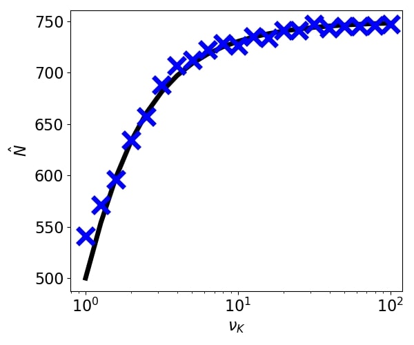
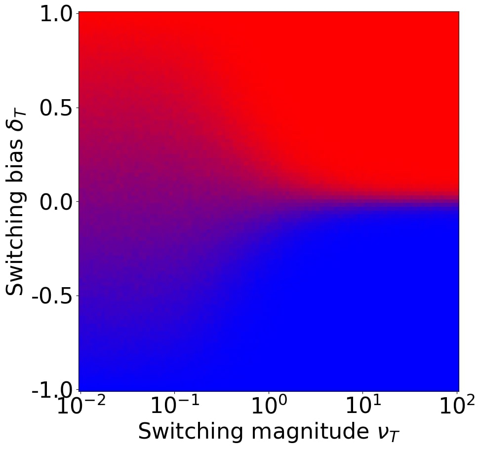
SM7. Videos of sample paths

Figure S5: Typical sample paths of $N,N_{R}$ and $N_{S}$ with colours magenta, blue, and red, respectively. Carrying capacity $K(t)$ is plotted in grey except in (d) where $K$-switching is very fast. Grey background indicates high toxin ($\xi_{T}=-1$) while white background indicates low toxin ($\xi_{T}=+1)$. Parameters are given by the quadruple $(s,\nu_{T},\delta_{T},\nu_{K})$, with $\delta_{K}=0.0$, $K_{-}=400$ and $K_{+}=2000$ in all panels, runs until either fixation occurs or $t=2K_{0}(1+\gamma\delta_{K})=2400$. (a) $(0.5,0.5,0.0,0.2)$, (b) $(0.5,10.0,-0.15,5.0)$, (c) $(0.5,10.0,0.15,0.05)$, (d) $(0.5,10.0,0.0,50.0)$, (e)-(f) $(0.5,10.0,0.1,5\times 10^{-6})$. In (b) $R$ fixates; in (a,c,e) there is fixation of $S$; in (d,f) there is long-lived coexistence; see text for details.

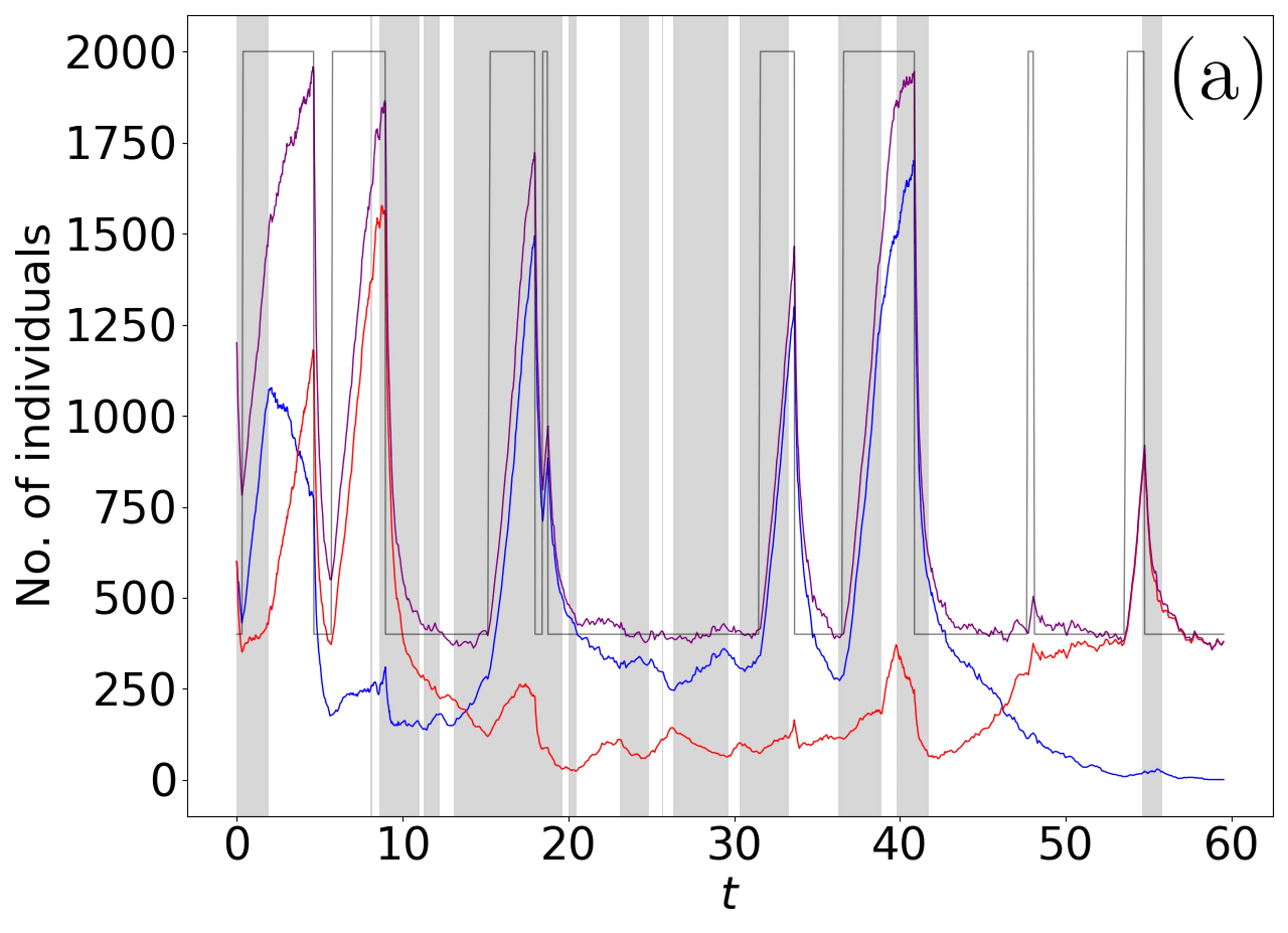
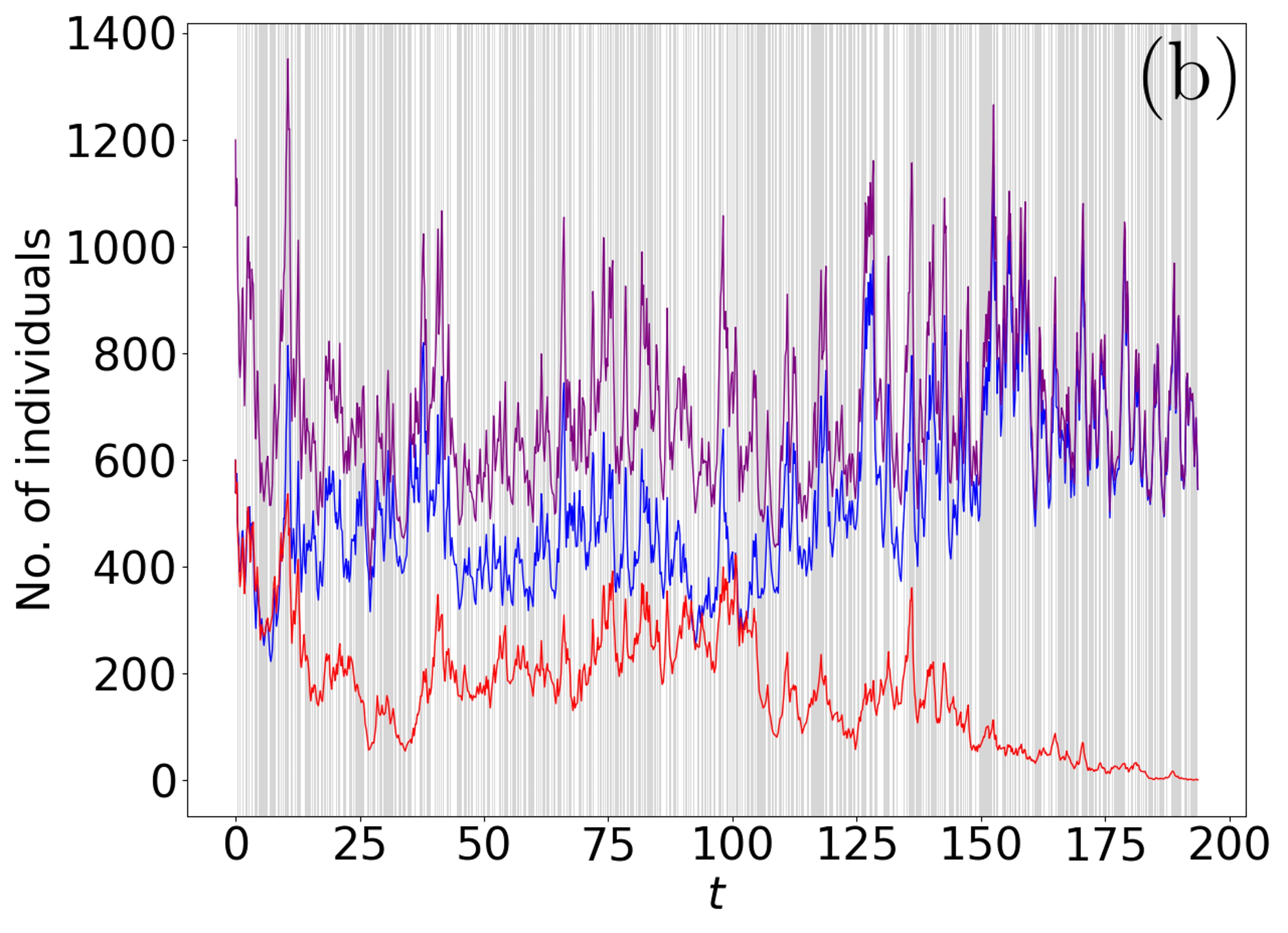
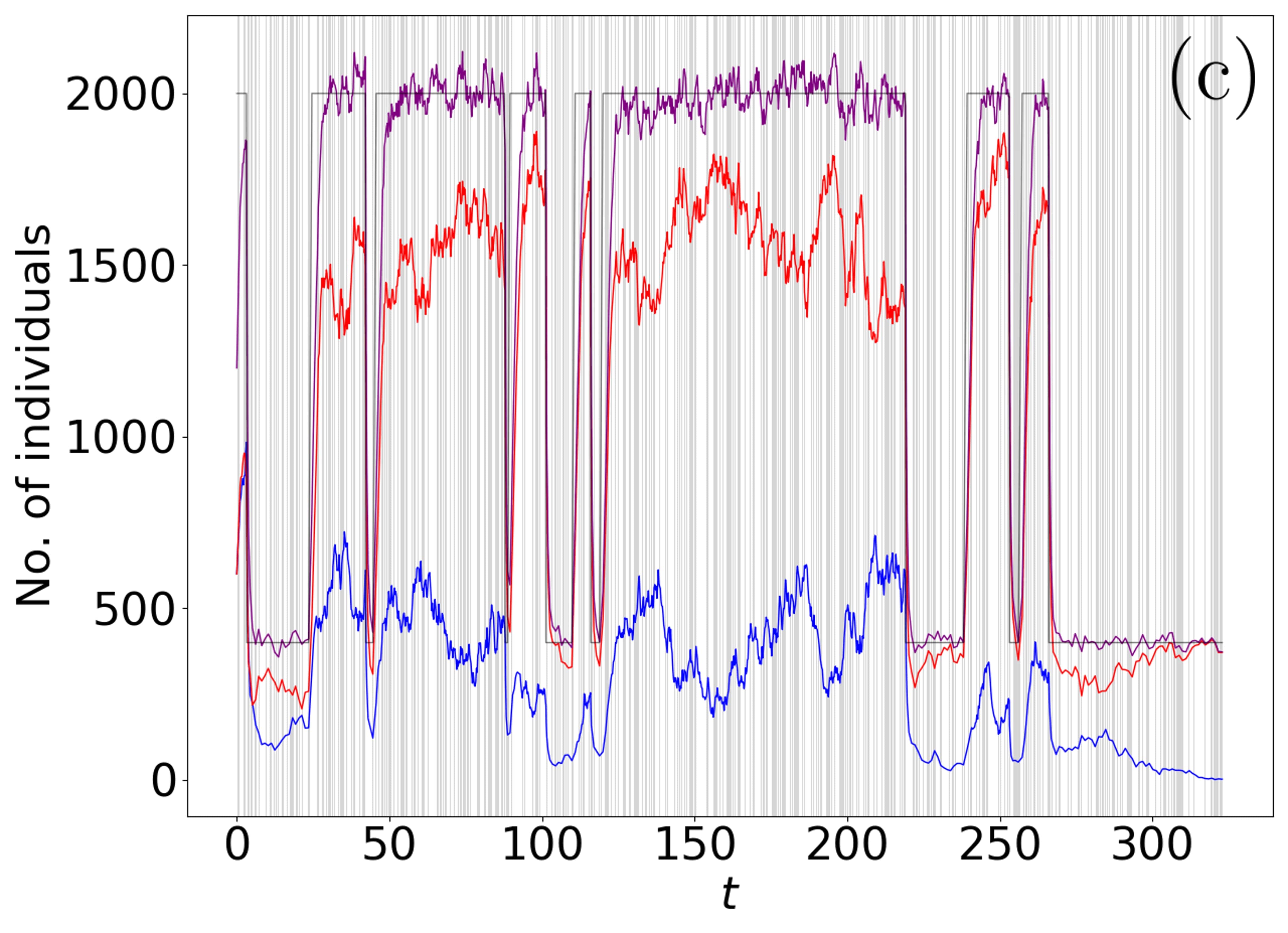
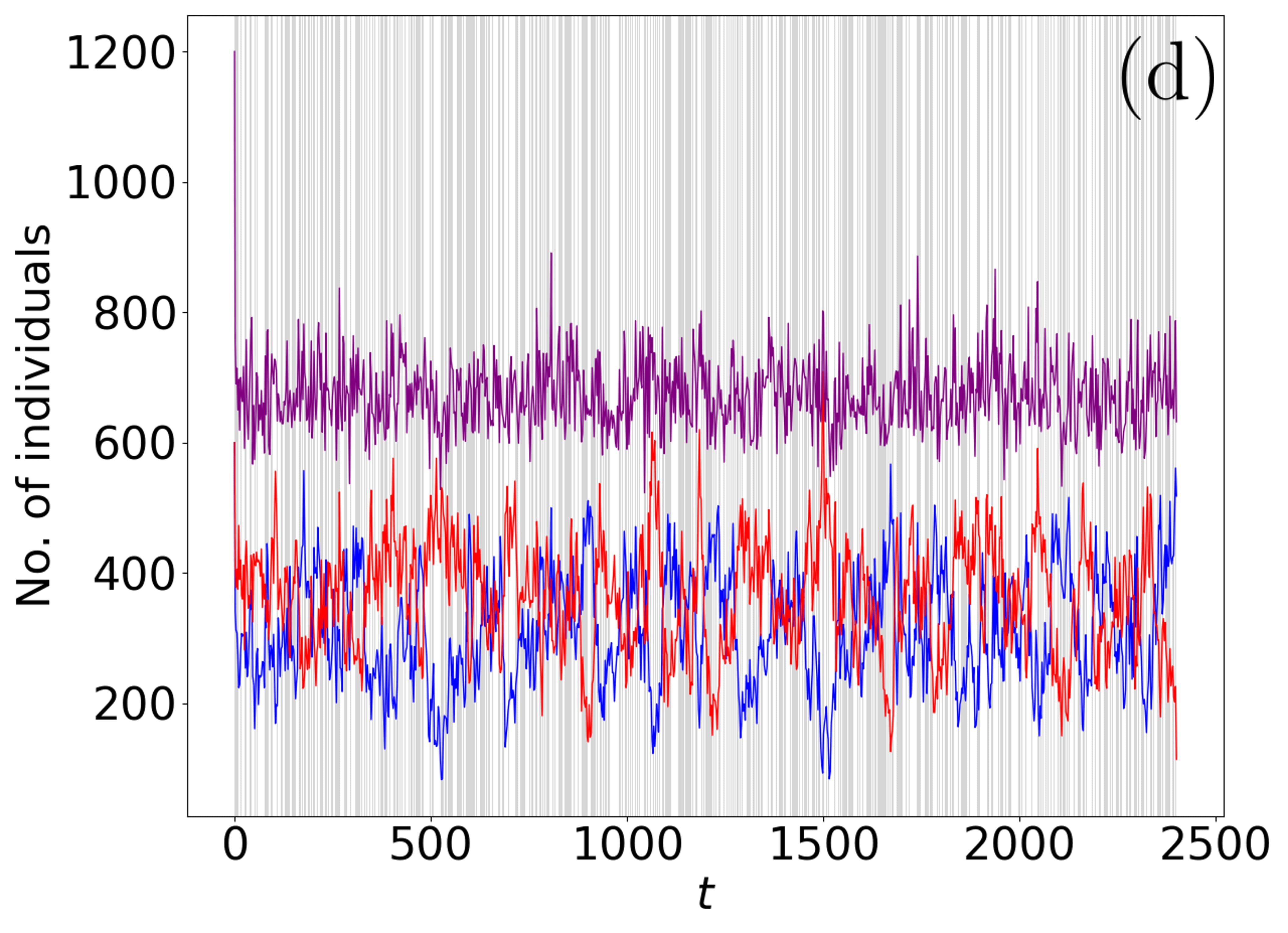
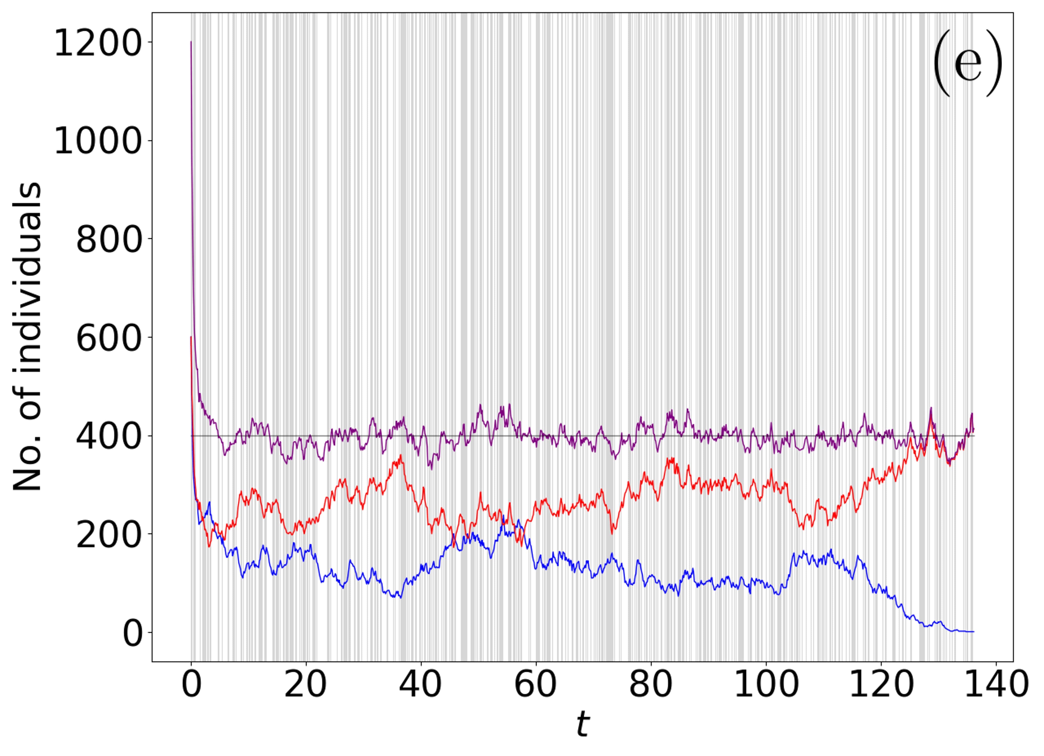
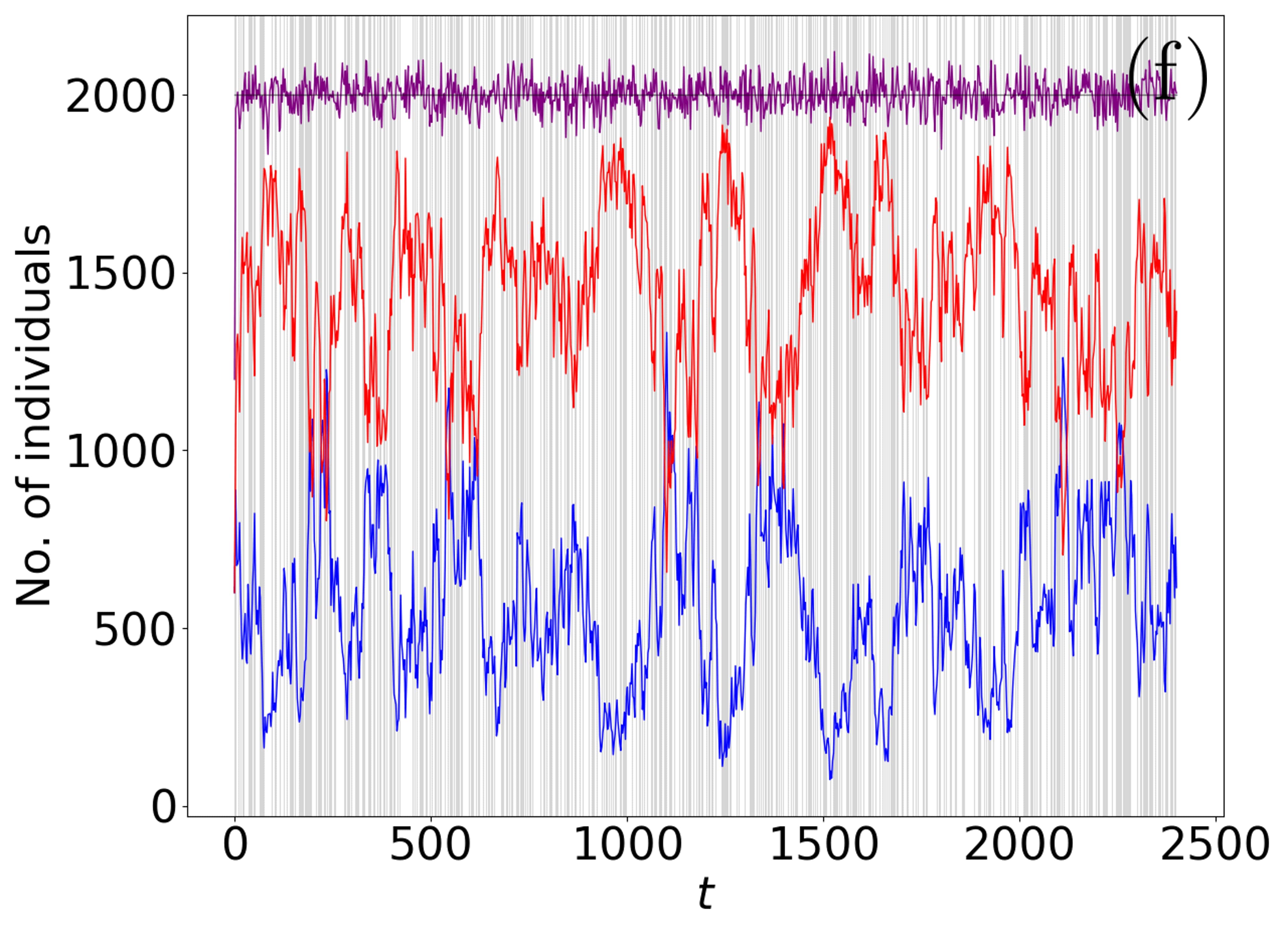
In this section we provide example trajectories for representative realisations of the full model under both fluctuations in the toxin level and in the carrying capacity. The corresponding movies are provided online in [111].

Fig. S5 captures the dynamics of the system in six example realisations under different EV parameters $(\nu_{T},\delta_{T},\nu_{K})$ for a selection strength $s=0.5$, which sets the magnitude of $T$-EV; and mean carrying capacity $K_{0}=1200$ with $\gamma=2/3$ ($K_{-}=400$ and $K_{+}=2000$), setting the magnitude of $K$-EV. For simplicity, we keep $\delta_{K}=0$.

- The example of Fig. S5(a) illustrates an unbiased fluctuating environment with intermediate $T$-switching rate (white background: low toxin level, grey: high toxin level; $\nu_{T}=0.5$, $\delta_{T}=0$) and $K$-switching rate (solid black line; $\nu_{K}=0.2$). We notice that total population $N$ rapidly attains quasi-stationarity well before a fixation event occurs ($S$ fixation in this example).

- In Fig. S5(b), we show faster environmental $T$ and $K$ switching, with $\nu_{T}=10$ and $\nu_{K}=5$. There is also a bias towards the harsh $T$ state favouring the strain $R$ ($\delta_{T}=-0.15$, high toxin level) that is responsible for a robust offset in strain abundance eventually leading to extinction of $S$ and fixation of $R$.

In this example, the $K$-EV switching rate is sufficiently high to ensure its self-averaging: in this fast $K$ switching regime, the population size is distributed about the effective carrying capacity $\mathcal{K}=K_{0}(1-\gamma^{2})/(1-\gamma\delta_{K})$ (here $N\approx\mathcal{K}=667$), see Fig. 4 and Sec. IV A.

- Fig. S5(c) illustrates the case of fast $T$-EV ($\nu_{T}=10$) with a bias towards the mild/low $T$ state favouring the strain $S$ ($\delta_{T}=0.15$). In this example, the $K$-EV switching rate is low ($\nu_{K}=0.05$) and the population size $N$ follows $K(t)$ and fluctuates about $K_{-}$ and $K_{+}$. The $T$-EV bias ($\delta_{T}>0$) is here responsible for a systematic offset in the strain abundance, with $N_{S}>N_{R}$, resulting in the fixation of $S$ and extinction of $R$, see Fig. 2(a). In this example, $K$-EV is responsible for larger demographic fluctuations in the environmental state $\xi_{K}=-1$, where $N\approx K_{-}$ and $S$ fixation is more likely than when $N\approx K_{+}$ ($\xi_{K}=+1$).

- Fig. S5(d) shows typical trajectories in the long-lived coexistence phase in the case of unbiased fast switching $T$-EV and $K$-EV, with $\nu_{T}=10,\delta_{T}=0$ and $\nu_{K}=50$. This set of parameters essentially corresponds (here $\nu_{K}=50$ instead of $\nu_{K}=5$) to a point in the bright green region in the diagram of Fig. 5(c), where $\eta\approx 1$ and long-lived coexistence is almost certain. As in panel (b), the fast $K$ switching (solid black line not shown in Fig. S5(d)) leads to fluctuations of the total population size about ${\cal K}$, i.e. $N\approx\mathcal{K}=667$. In this example $x^{*}=1/2$, see Fig. 7, and the number of $R$ and $S$ cells fluctuates about their averages: $\left\langle N_{R}\right\rangle\approx\left\langle N_{S}\right\rangle\approx{\cal K}/2\approx 333.5$, see Sec. V B.

- Fig. S5(e,f) illustrate the dynamics under fast $T$-EV ($\nu_{T}=10$) and extremely slow $K$-switching rate ($\nu_{K}=5\times 10^{-6}$), with an initial carrying capacity $K(0)=K_{-}$ in (e) and $K(0)=K_{+}$ (f). There is also a small bias towards the mild $T$ state favouring $S$ ($\delta_{T}=0.1$). This choice of parameters corresponds to a point in the faint green region in the diagram of Fig. 5(a), where $0<\eta<1$ and long-lived coexistence is possible but not certain. In panel (e), the population size fluctuates about $K(0)=K_{-}$ ($N\approx K_{-}$) and is not able to sustain long-lived coexistence: demographic fluctuations yield $S$ fixation in a time $t\lesssim 2K_{-}=800$. In panel (f), we have $N\approx K_{+}$ and, as demographic fluctuations are unable to cause the fixation/extinction of either strain in a time less than $2\left\langle N\right\rangle=2K_{+}=4000$ (for clarity, the time series in Fig. S5 have been truncated at $t=2400$), we have long-lived coexistence.

In all examples in the panels of Fig. S5, the population size $N$ reaches quasi-stationarity (settles in the QPSD) a significant time before the fixation of one strain and extinction of the other, in line with the considerations underpinning Eqs. (19) and (20).

SM8. Fully correlated and anti-correlated environmental variability

Figure S6: Top to bottom: uncorrelated, fully correlated and fully anticorrelated case heatmap plots from $10^{3}$ realisations with $\gamma=0.9$ (correlated: $\widetilde{\gamma}=0.9$, anticorrelated: $\widetilde{\gamma}=-0.9$). Left to right we have $s\in\{0.2,2,20\}$ and use $K_{0}=1000$. In the uncorrelated case we have $\nu_{K}=0.0001$ and $\delta_{K}=0.0$. Considering the correlated case, in the coexistence region, for $\delta\to+1$ and fast-switching $\nu\gtrsim 1$ the effective carrying capacity increases. Therefore, we see the coexistence region extended further towards $\delta=1$. For $\delta\to-1$ and $\nu\gtrsim 1$ we find the converse where the effective carrying capacity decreases and thus the coexistence region shrinks away from $\delta=-1$. A similar logic applies to the anticorrelated case; see text. Color (greyscale) coding is the same as in Fig. 3.

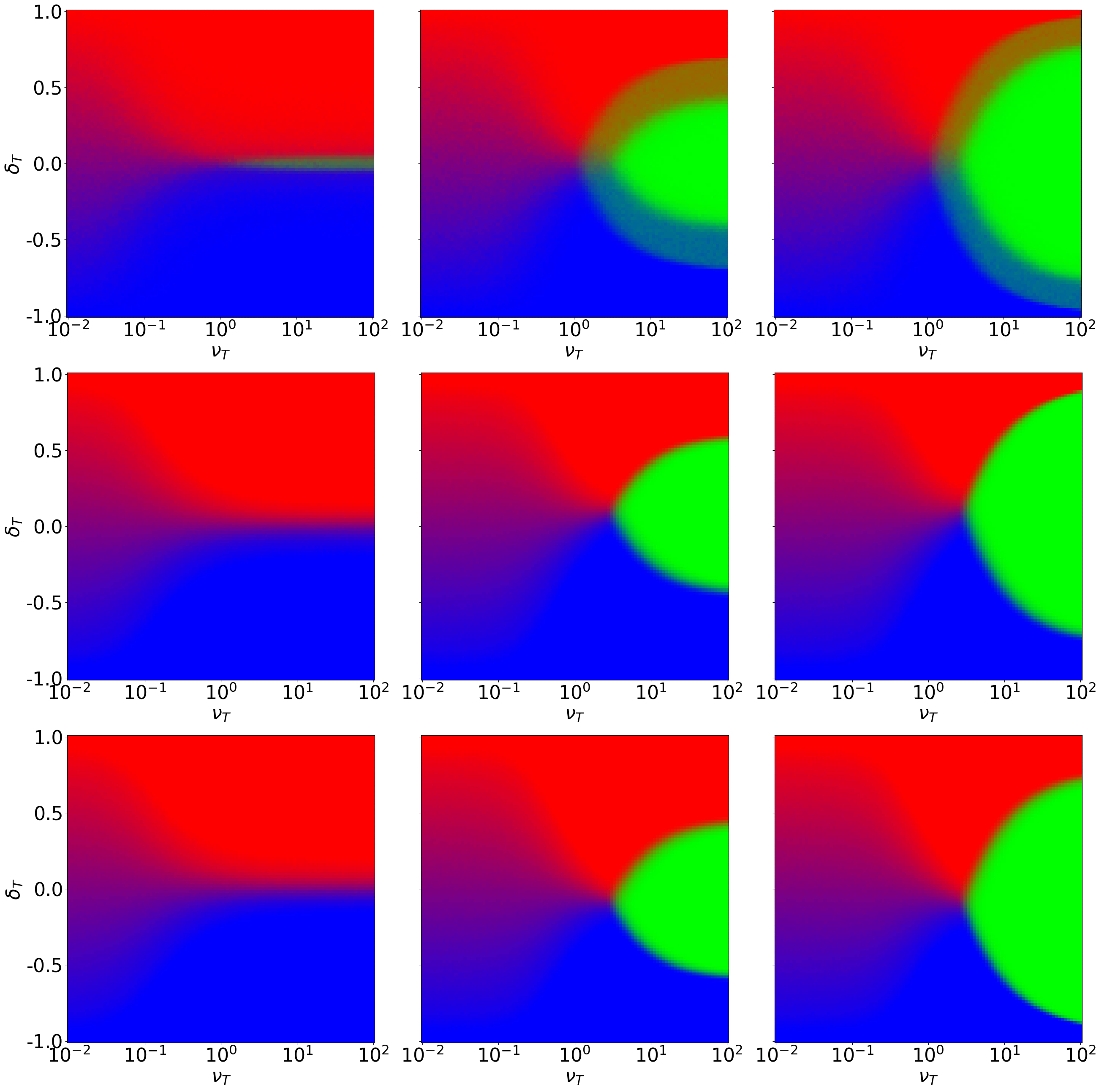
In the case of fully correlated/anti-correlated $T$-EV and $K$-EV, environmental variability is no longer twofold since we have $\xi\equiv\xi_{T}$ and $\xi_{K}=\xi$ (fully correlated EV) or $\xi_{K}=-\xi$ (fully anti-correlated EV). The switching carrying capacity can thus be written as

$$K(t)=K_{0}[1+\widetilde{\gamma}\xi(t)],$$

where $\widetilde{\gamma}=\gamma$ in the fully correlated case, and $\widetilde{\gamma}=-\gamma$ when $T$-EV and $K$-EV are fully anti-correlated. For instance, this implies that, in the correlated case, the environmental state $\xi=+1$ corresponds to $f_{s}=e^{s}>1$ and $K=K_{+}$ (low toxin level, abundant resources), while $\xi=-1$ is associated with $f_{S}=e^{-s}<1$ and $K=K_{-}$ (high toxin level, scarce resources). As said, under fully correlated/anti-correlated $T/K$-EV, environmental variability is no longer twofold: $\xi$ simultaneously drives the level of toxin and the abundance of resources. Hence, we can characterise the effect of fully correlated/anti-correlated EV in terms of $\nu\equiv\nu_{T}$ and $\delta\equiv\delta_{T}$, and the fully anti-correlated case is related to completely correlated EV via $\widetilde{\gamma}\to-\widetilde{\gamma}$. An example of fully-anticorrelated EV modelled in terms of a dichotomous process driving the level of toxins and resources in the context of competitive exclusion is considered in [65].

Fig. S6 shows the comparison between the uncorrelated $T$-EV and $K$-EV studied in the main text (top row), and the fully correlated (middle row) and fully anti-correlated (bottom row) cases reported here, all under $K_{0}=1000$ and $\gamma=0.9$, and for different selection strengths $s\in\{0.2,2,20\}$ (left to right columns). For the uncorrelated case, the parameters of $K$-EV are independent from those of $T$-EV parameters, and are here chosen to be $(\nu_{K},\delta_{K})=(10^{-4},0)$, i.e. unbiased slow-switching $K$-EV (similar to the example of Fig. 5(a)).

Since the fully correlated and anti-correlated cases (middle and bottom rows) are mirror images through the horizontal axis (symmetric with respect to $\delta_{T}=0$) and under a red-blue colour change, we focus on the correlated case only (middle row). For this case, $\widetilde{\gamma}=\gamma=0.9$, with $\xi_{K}=\xi_{T}\equiv\xi$, $\nu_{K}=\nu_{T}$, and $\delta_{K}=\delta_{T}$. In the fully correlated case, we observe that both the blue (resistant fixation) and the bright green (coexistence) regions shift upwards (to higher toxin level biases $\delta_{T}$) as the selection strength increases (from left to right column). We can understand this phenomenon in light of the $T$-correlated $K$-EV fluctuations. This is, since $\delta_{K}=\delta_{T}$, a lower value of $\delta_{T}$ in the diagrams implies longer cumulative periods in the harsh toxin level, but also in the low carrying capacity environment. Therefore, lower $\delta_{T}$ provides the selective advantage to resistant strain at the same time that it shrinks the total population. Demographic fluctuations being stronger in smaller populations, correlated $T$-EV and $K$-EV thus provide higher $R$ fixation probability (blue region shifted up), as well as lower coexistence probability (green region shifted up). Moreover, since total population increases with the bias towards positive carrying (here $\delta_{K}=\delta_{T}$), see Sec. IV A, the MFT thus increases with $\delta_{T}$ (see Fig. 2(c)), and the coexistence probability thus shifts upwards. The magnitude of the upwards shift in the correlated case, is small but increases with selection strength $s$ that increases the amplitude of the $T$-EV fluctuations.

In summary, we obtain the same qualitative results for fully correlated/anti-correlated $T/K$-EV as when $\xi_{T/K}$ are independent (uncorrelated environmental noise, twofold EV), with some minor quantitative differences, as shown in Fig. S6 and discussed above. We conclude that the similar behaviour observed for uncorrelated and (anti-)correlated $T/K$-EV indicates that our findings are robust against the detailed model specifications: the results are expected to be valid for the general case of twofold environmental variability where $T/K$-EV are neither completely independent nor fully correlated/anti-correlated.