Tackling Computational Heterogeneity in FL:
A Few Theoretical Insights

Abstract

The future of machine learning lies in moving data collection along with training to the edge. Federated Learning, for short FL, has been recently proposed to achieve this goal. The principle of this approach is to aggregate models learned over a large number of distributed clients, i.e., resource-constrained mobile devices that collect data from their environment, to obtain a new more general model. The latter is subsequently redistributed to clients for further training. A key feature that distinguishes federated learning from data-center-based distributed training is the inherent heterogeneity. In this work, we introduce and analyse a novel aggregation framework that allows for formalizing and tackling computational heterogeneity in federated optimization, in terms of both heterogeneous data and local updates. Proposed aggregation algorithms are extensively analyzed from a theoretical, and an experimental prospective.

Keywords: Federated Learning, Model Aggregation, Heterogeneity

1 Introduction

Until recently, machine learning models were extensively trained in centralized data center settings using powerful computing nodes, fast inter-node communication links, and large centrally-available training datasets. However, with the proliferation of mobile devices that collectively gather a massive amount of relevant data every day, centralization is not always practical [Lim et al. (2020)]. Therefore, the future of machine learning lies in moving both data collection and model training to the edge to take advantage of the computational power available there, and to minimize the communication cost. Furthermore, in many fields such as medical information processing, public policy, and the design of products or services, the collected datasets are privacy-sensitive. This creates a need to reduce human exposure to data to avoid confidentiality violations due to human failure. This may preclude logging into a data center and performing training there using conventional approaches. In fact, conventional machine learning requires feeding training data into a learning algorithm and revealing information indirectly to the developers. When several data sources are involved, a merging procedure for creating a single dataset is also required, and merging in a privacy-preserving way is still an important open problem [Zheng et al. (2019)].

Algorithm 1 General Federated Learning Protocol

Input: N, C, T, E
Output: $w_{TE}$

1:  Initialize $w_{0}$.

2:  for each round $t\in\{0,E,2E,\dots,(T-1)E\}$ do

3:     $m\leftarrow\max(C\cdot N,1)$

4:     $I_{t}\leftarrow$Create-Client-Set$(m)$

5:     for each client $i\in I_{t}$ in parallel do

6:        $w_{t+E}^{i}\leftarrow\text{{Client-Update}}(w_{t})$

7:     end for

8:     $w_{t+E}\leftarrow\text{{Aggregation}}(w_{t+E}^{1},\dots,w_{t+E}^{N})$

9:  end for

10:  return $w_{TE}$

Recently, McMahan et al. (2017b) proposed a distributed data-mining technique for edge devices called Federated Learning (FL), which allows to decouple the model training from the need for direct access to the raw data. Formally, FL is a protocol that operates according to Algorithm 1, cf. Li et al. (2020b) for an overview. The framework involves a group of devices called clients and a server that coordinates the learning process. Each client has a local training dataset that is never uploaded to the server. The goal is to train a global model by aggregating the results of the local training. Parameters fixed by the centralized part of the global learning system include: $N$ clients, the ratio of clients $C$ selected at each round, the set of clients $I_{t}$ selected at round $t$, the number of communication rounds $T$, and the number of local epochs $E$. A model for a client $i$ at a given instant $t$ is completely defined by its weights $w_{i}^{t}$. At the end of each epoch $t\in\{0,\dots,TE-1\}$, $w_{t+1}^{i}$ indicates the weight of client $i\in I$. For each communication round $t\in\{0,E,\dots,(T-1)E\}$, $w_{t}$ is the global model detained by the server at time $t$, and $w_{TE}$ is the final weight. In the following, we will use the notations given in Table 1.

Table 1: Conventions used in this paper.

Notation	Meaning
$N$	number of clients
$C$	ratio of clients
$I_{t}$	set of clients selected at round $t$
$T$	number of communication rounds
$E$	number of local epochs
$w_{t}$	weights of the global model at time $t$
$w_{t}^{i}$	model of client $i$ at time $t$
$F_{i}^{t}$	loss function of the $i$-th client at time $t$
$F$	averaged loss function at time $t$
$\eta_{t}$	learning rate decay at time $t$
$\zeta_{t}^{i}$	mini-batch associated to client $i$ at time $t$
∗	index of optimality

Algorithm 1 describes the training procedure for FL. The framework involves a fixed set of $I=\{1,\dots,N\}$ clients, each with a local dataset. Before every communication round $t\in\{0,E,\dots,(T-1)E\}$, the server sends the current global model state to the clients and requests them to perform local computations based on the global state and their local dataset, and sends back an update. At the end of each round, the server updates the weights of the model by aggregating the clients’ updates, and the process repeats. For the client selection procedure (Create-Client-Set), local training procedure (Client-Update), and aggregation of the local updates (Aggregation), several possibilities exist. For some results concerning client selection, see [McMahan et al. (2017a); Chen et al. (2017); Huang et al. (2022); Cho et al. (2022b)]. Regarding local updates, available methods range from simple variants of SGD, such as mini-batch SGD [Gower et al. (2019)], to more sophisticated approaches, such as PAGE [Zhao et al. (2021)]; other results are included in [Berahas et al. (2022); Liu et al. (2020); Reddi et al. (2020); Jin et al. (2022)]. We will describe in greater detail the existing routines for aggregation, the central topic of this work. In 2017, the seminal work of McMahan et al. (2017b) proposed a plain coordinate-wise mean averaging of model weights; later, Yurochkin et al. (2019) proposed an extension that takes the invariance of network weights under permutation into account. The same year, Bonawitz et al. (2019) proposed an auto-tuned communication-efficient secure aggregation. More recently, Cho et al. (2020) extended the coordinate-wise mean averaging approach, substituting it with a term that amplifies the contribution of the most informative terms over less informative ones. Then, Sannara et al. (2021) adjusted this to enforce closeness of local and global updates. Last year, Charles et al. (2022) introduces an aggregation that allows clients to select what values of the global model are sent to them. Despite methodological advances, there is neither theoretical nor practical evidence for the right criterion for choosing a particular aggregation strategy.

Figure 1: Simplified representation of classic FL framework.

1.1 The Challenges from Computational Heterogeneity in FL

As we have seen above, several emerging FL algorithms have been proposed. Due to the high cost of real deployment, existing studies in FL usually involves simulations [Li et al. (2019); Chen et al. (2019); Bagdasaryan et al. (2020)] and have no data to describe how devices participate in FL [Yang et al. (2021)]. The direct consequence of this approach is that this studies build on excessively ideal assumptions, for instance the one that all the devices are constantly available for training and equipped with the same resources, e.g., the same CPU and RAM capacity [Li et al. (2019); Chen et al. (2019); Bagdasaryan et al. (2020); Mohri et al. (2019); Konečnỳ et al. (2016)]. However, these assumptions can be inadequate for FL deployment in practice. FL, in fact, requires a large number of devices to collaboratively accomplish a learning task, which poses a great challenge, namely heterogeneity [Li et al. (2020a)], that impacts FL both in terms of accuracy and training time. We can divide heterogeneity in two main macro-classes: the system heterogeneity and the statistical heterogeneity.

In federated settings, system heterogeneity points out the significant variability in the systems characteristics across the network, as devices may differ in terms of hardware, network connectivity, and battery power. These systems characteristics make issues such as stragglers significantly more prevalent than in typical data center environments. Several solution to handle systems heterogeneity have been proposed, e.g. asynchronous communication, see [Dai et al. (2015); Duchi et al. (2013)], active device sampling, see [Nishio and Yonetani (2019)], and fault tolerance, see [Jiang and Agrawal (2018)]. Statistical heterogeneity deals instead with the challenges that arise when training federated models from data that is not identically distributed across devices, both in terms of modeling the data, and in terms of analyzing the convergence behavior of associated training procedures. There exists a large body of literature in machine learning that has modeled statistical heterogeneity via methods such as meta-learning and multi-task learning [Chen et al. (2018); Corinzia et al. (2019); Eichner et al. (2019); Khodak et al. (2019)].

Despite heterogeneity is associated with several possible problems such as free-riding [Karimireddy et al. (2022)], theoretical guarantee to convergence of heterogeneous federated learning have been recently found [Zhou et al. (2022, ); Wang et al. (2020)] and approaches to overcome these challenges formalized, e.g. thanks to the introduction of Personalized Federated Learning (PFL) [Tan et al. (2022); Bergou et al. (2022); Cho et al. (2021)], and the one of heterogeneous ensemble knowledge transfer [Cho et al. (2022a)]. Several methods have been proposed to attack the heterogeneity arising from specific sources such as data, see [Shang et al. (2022); Horváth et al. (2022); Mendieta et al. (2022)], partial and biased client participation, see [Jhunjhunwala et al. (2022); Cho et al. (2022b)]. In what follows, we will discuss how to possibly tackle heterogeneous local updates performances in edge clients, propose new aggregation methods, test them experimentally, and provide insights on their convergence properties, their stability and the client participation within the training.

2 Tackling Performance-Heterogeneity in FL: The Theoretical Side

We study theoretically how the heterogeneous performances of clients can be exploited in aggregation methods (under reasonable assumptions). The analysis presented is fairly general and allows to extract information concerning the existing trade-off between accuracy and efficacy. This analysis can be seen as a remarkable follow-up of Cho et al. (2020), the first work presenting a convergence analysis of federated learning with biased client selection that is cognizant of the training progress at each client, and the work where was discovered that biasing the client selection towards clients with higher local losses increases the rate of convergence (compared to unbiased client selection).

2.1 Framework of Analysis & Preliminaries

Throughout the analysis, we assume that all the clients are involved in each local and global iteration, i.e., $C=1$. We denote with $F_{i}$ the loss function of the $i$-th client, and with $F$ the weighted average of the $F_{i}$ upon the distribution $P:=\{p_{i}\mid i\in I\}$. We restrain our analysis to the case in which the Client-Update procedure is mini-batch SGD with learning rate decay $\eta_{t}$ and mini-batches $\zeta_{t}^{i}$ of cardinality $b$. In particular:

$$g_{i}(w_{t}^{i}):=\frac{1}{b}\sum\limits_{\zeta\in\zeta_{t}^{i}}\nabla F_{i}(w_{t}^{i},\zeta)$$ (1)

In any iteration, the weights of the model are defined as follows:

$$w_{t+1}^{i}:=\left\{\begin{array}[]{ll}\displaystyle w_{t}^{i}-\eta_{t}g_{i}(w_{t}^{i})&\mbox{if }E\not{|}t\\ \\ \displaystyle\sum_{j\in I}\alpha_{t}^{j}(w_{t}^{j}-\eta_{t}g_{j}(w_{t}^{j})):=w_{t+1}&\mbox{if }E|t\end{array}\right.$$ (2)

where $\alpha_{t}^{j}$ is the aggregation coefficient referred to client $j$ at communication round $t$, and where, for each $t$, the following constraint holds:

$$\sum\limits_{j\in I}{\alpha_{t}^{j}}=1$$ (3)

In our mathematical analysis, we introduce a few assumptions:
Assumption 1 ($L$-smoothness) $F_{1},\dots,F_{N}$ satisfy:

$\forall v,w$, $F_{i}(v)\leq F_{i}(w)+\left\langle v-w,\nabla F_{i}(w)\right\rangle+\frac{L}{2}\left\lVert v-w\right\rVert_{2}^{2}$

Assumption 2 ($\mu$-convexity) $F_{1},\dots,F_{N}$ satisfy:

$\forall v,w$, $F_{i}(v)\geq F_{i}(w)+\left\langle v-w,\nabla F_{i}(w)\right\rangle+\frac{\mu}{2}\left\lVert v-w\right\rVert_{2}^{2}$

Assumption 3 The variance of the stochastic gradient descent is bounded, more formally, the following condition is satisfied:

$\forall i\in I$, $\mathds{E}\left\lVert g_{i}(w_{i})-\nabla F_{i}(w_{i})\right\rVert^{2}\leq\sigma^{2}$

Assumption 4 The stochastic gradient’s expected squared norm is uniformly bounded, in mathematical terms:

$\forall i\in I$, $\mathds{E}\left\lVert g_{i}(w_{i})\right\rVert^{2}\leq G^{2}$

What follows is closely related to what was previously done in Cho et al. (2022b), the novelty arise from the fact that: (a) instead of analyzing the selection of clients, we examine the attribution of the weights to them, and (b) we extensively study the expression of the learning error from which we derive principled aggregation strategies.
To facilitate the convergence analysis, we define the quantity $w_{t}$ (for which $t\neq 0\bmod E$) as:

$$w_{t+1}:=w_{t}-\eta_{t}\sum\limits_{i\in I}\alpha_{t}^{i}g_{i}(w_{t}^{i})$$ (4)

where $\alpha_{t}^{i}=p_{i}$. Let $w^{\star}$ be the global optimum of $F$ and $w^{\star}_{i}$ the global optimum of $F_{i}$. We define $F^{\star}$ as $F(w^{\star})$, $F^{\star}_{i}$ as $F(w^{\star}_{i})$ and heterogeneity as:

$$\Gamma:=F^{\star}-\sum_{i\in I}p_{i}F_{i}^{\star}$$ (5)

We list below a couple of results useful in proving the main theorem.

Lemma 1

Let $f$ be a $L$-smooth function with a unique global minimum at $w^{\star}$. Then :

$$\forall w,\hskip 28.45274pt||\nabla f(w)||^{2}\leq 2L(f(w)-f(w^{\star}))$$ (6)

Lemma 2

With the same notations as above and defining $\mathds{E}[.]$ as the total expectation over all random sources, the expected average discrepancy between $w_{t}$ and $w_{t}^{i}$ is bounded:

$$\mathds{E}\left[\sum_{i\in I}\alpha_{t}^{i}\left\lVert w_{t}-w_{t}^{i}\right\rVert^{2}\right]\leq 16\eta_{t}^{2}E^{2}G^{2}$$ (7)

Before presenting the main results, we define the weighting skew $\rho$ as:

$$\rho(t,w):=\frac{\sum\limits_{i\in I}\alpha_{t}^{i}(F_{i}(w)-F_{i}^{\star})}{F(w)-\sum\limits_{i\in I}p_{i}F_{i}^{\star}}$$ (8)

and introduce these notations: $\overline{\rho}:=\min\limits_{t=0\mod E}\leavevmode\nobreak\ \rho(t,w_{t})$, and $\tilde{\rho}:=\underset{t=0\mod E}{\max}\leavevmode\nobreak\ \rho(t,w^{\star})$.

2.2 Main Theorem and Consequences

In the framework outlined, we state an extension of the main theorem presented in Cho et al. (2022b), that is adapted to our extended goal. The proofs are available in the appendix A.

Theorem 3

Under assumptions (1 - 4), the following holds:

$$\mathds{E}\left[\left\lVert w_{t+1}-w^{\star}\right\rVert^{2}\right]\leq\left(1-\eta_{t}\mu\left(1+\frac{3}{8}\overline{\rho}\right)\right)\mathds{E}\left[\left\lVert w_{t}-w^{\star}\right\rVert^{2}\right]$$

$$+\eta_{t}^{2}\left(32E^{2}G^{2}+6\overline{\rho}L\Gamma+\sigma^{2}\right)$$ (9)

$$+2\eta_{t}\Gamma\left(\tilde{\rho}-\overline{\rho}\right)$$

From Theorem 3, we can directly deduce Corollary 4 below.

Corollary 4

Assuming $\eta_{t}=\frac{1}{\mu(t+\gamma)}$ and $\gamma=\frac{4L}{\mu}$, the following bound holds:

$$\mathds{E}[F(w_{T})]-F^{\star}\leq\frac{1}{T+\gamma}\mathcal{V}(\overline{\rho},\tilde{\rho})+\mathcal{E}(\overline{\rho},\tilde{\rho})$$ (10)

where:

$$\mathcal{V}(\overline{\rho},\tilde{\rho})=\frac{4L(32\tau^{2}G^{2}+\sigma^{2})}{3\mu^{2}\overline{\rho}}+\frac{8L^{2}\Gamma}{\mu^{2}}+\frac{L\gamma\left\lVert w^{0}-w^{\star}\right\rVert^{2}}{2}$$

$$\mathcal{E}(\overline{\rho},\tilde{\rho})=\frac{8L\Gamma}{3\mu}\left(\frac{\tilde{\rho}}{\overline{\rho}}-1\right)$$

Remark 5

Corollary 4 implies that:

$$\mathbb{E}[F(w_{T})-F^{\star}]=O(1/T)$$ (11)

The mathematical expressions $\mathcal{V}$ and $\mathcal{E}$ are estimators for the speed of convergence, and the learning error, respectively. A complex multi-objective optimization problem arises when trying to maximize the speed while minimizing the error. We decouple these two quantities and optimize them separately without underestimating the existing trade-off among them. This procedure allows to outline the global trends, but it does not imply the universal optimality of the strategies defined below.

Remark 6

Since $\frac{8L^{2}\Gamma}{\mu^{2}}+\frac{L\gamma\left\lVert w^{0}-w^{\star}\right\rVert^{2}}{2}$ is a constant depending only on the data and the initial guess, and $\overline{\rho}$ may be arbitrary large, we can deduce from Corollary 4 the existence of a minimal value for the convergence speed, given by:

$$\mathcal{V}_{\min}:=\frac{8L^{2}\Gamma}{\mu^{2}}+\frac{L\gamma\left\lVert w^{0}-w^{\star}\right\rVert^{2}}{2}$$ (12)

In this framework, we can analyze all the possible scenarios, starting from the one in which $\Gamma=0$, that can be appointed as error-free case and corresponds to an IID-dataset.

Error-free Framework

Under the assumption that $\Gamma=0$, the main theorem can be leveraged as follows:

$$\mathds{E}\left[\left\lVert w_{t+1}-w^{\star}\right\rVert^{2}\right]\leq\left(1-\eta_{t}\mu\left(1+\frac{3}{8}\overline{\rho}\right)\right)\mathds{E}\left[\left\lVert w_{t}-w^{\star}\right\rVert^{2}\right]+\eta_{t}^{2}\left(32E^{2}G^{2}+\sigma^{2}\right)$$ (13)

and applying Corollary 4, we derive the following inequality:

$$\mathds{E}[F(w_{T})]-F^{\star}\leq\frac{1}{T+\gamma}\left[\frac{4L(32\tau^{2}G^{2}+\sigma^{2})}{3\mu^{2}\overline{\rho}}+\frac{L\gamma\left\lVert w^{0}-w^{\star}\right\rVert^{2}}{2}\right]$$ (14)

Despite its simplicity, this setting is interesting since the error term vanishes, and therefore we can deduce a truly optimal algorithm given by the maximization of $\overline{\rho}$: , achieved when:

$$\alpha_{t}^{i}=\left\{\begin{array}[]{ll}\displaystyle\frac{1}{|J_{t}|}&\mbox{if }i\in J_{t}\\ \\ \displaystyle 0&\mbox{else }\end{array}\right.$$ (15)

where $J_{t}=\underset{i\in I}{\operatorname*{arg\,max}}(F_{i}(w_{t})-F_{i}^{\star})$.

General Framework

In the general case, both $\mathcal{V}$ and $\mathcal{E}$ depend on the choice of the $\alpha_{i}^{t}$. As already noticed before, this raises a multi-objective problem that doesn’t allow for a joint optimization of terms $\mathcal{V}$ and $\mathcal{E}$. Consequently, we provide an approximated optimization that builds upon the existing trade-off between the convergence speed and the accuracy.

Remark 7

We observe that optimizing the convergence speed, while ”forgetting” about the error, amounts to maximize $\overline{\rho}$, exactly as done in the error-free case. Instead, minimizing $\mathcal{E}(\overline{\rho},\tilde{\rho})$ neglecting $\mathcal{V}$, amounts to minimize $\frac{\tilde{\rho}}{\overline{\rho}}-1$. This is achieved when $\alpha_{t}^{i}=p_{i}$, which gives $\mathcal{E}=0$.

Now, knowing that $\alpha_{t}^{i}=p_{i}$ ensures obtaining optimal accuracy, we assume $\alpha_{t}^{i}=\kappa_{t}^{i}p_{i}$. The following notation is used:

$$\pi_{t}=\underset{i\in I}{\min}\leavevmode\nobreak\ \kappa_{t}^{i},\Pi_{t}=\underset{i\in I}{\max\leavevmode\nobreak\ }\kappa_{t}^{i},\pi=\underset{t}{\min}\leavevmode\nobreak\ \pi_{t},\text{ and }\Pi=\underset{t}{\max\leavevmode\nobreak\ }\Pi^{t}$$ (16)

Without loss of generality, we assume without that $\forall t,\pi_{t}>0$. If it were not the case, we would have assigned to the $\alpha_{t}^{i}$ equal to zero an infinitesimal value, and increment the other $\alpha_{t}^{i}$ substantially. Under these assumptions, we have that $\frac{\tilde{\rho}}{\overline{\rho}}\leq\frac{\Pi}{\pi}$, $\frac{1}{\overline{\rho}}\leq\frac{1}{\pi}$ and therefore:

$$\mathds{E}[F(w_{T})]-F^{\star}\leq\frac{1}{T+\gamma}\left[C+\frac{\lambda_{1}}{\pi}\right]+\lambda_{2}\frac{\Pi-\pi}{\pi}$$ (17)

where $C,\lambda_{1}$ and $\lambda_{2}$ are constants. Since,

$$\Pi\min\leavevmode\nobreak\ p_{i}\leq\max\leavevmode\nobreak\ \kappa_{t}^{i}p_{i}\leq 1-(N-1)\min\leavevmode\nobreak\ \kappa_{t}^{i}p_{i}\leq 1-(N-1)\pi\min\leavevmode\nobreak\ p_{i}$$ (18)

we can infer that $\Pi\leq\frac{1-(N-1)\pi\min\leavevmode\nobreak\ p_{i}}{\min\leavevmode\nobreak\ p_{i}}$ and $\mathcal{E}\leq\frac{1}{\pi\min\leavevmode\nobreak\ p_{i}}-N$, from which, we obtain:

$$\mathds{E}[F(w_{T})]-F^{\star}\leq\frac{1}{T+\gamma}\left[C+\frac{\lambda_{1}}{\pi}\right]+\lambda_{2}\left(\frac{1}{\pi\min\leavevmode\nobreak\ p_{i}}-N\right)$$ (19)

Remark 8

This last inequality has an intrinsic interest; in fact, it allows to state that the new speed and error bounds depend exclusively on $\pi$ and to ensure a bound on the error term (once set a properly chosen minimal value of the $\alpha_{t}^{i}$).

2.3 Derived Aggregation Strategies

The theoretical results discussed above provides several important insights for the design of aggregation algorithms.

The first algorithm presented is the generalized FedAvg, that corresponds to take $\alpha_{t}^{i}=p_{i}$ for any $t$ and $i\in I$. This strategy is inspired by McMahan et al. (2017b) and it boils down to consider the weighted average (upon $p_{i}$) of the local models as global model. As observed above, this approach is optimal in terms of accuracy (since $\mathcal{E}=0$) and its convergence speed can be bounded as below:

$$\mathcal{V}=\mathcal{V}_{\min}+\frac{4L-32\tau^{2}G^{2}+\sigma^{2}}{3\mu^{2}}$$ (20)

The second algorithm proposed is called FedMax and it is defined as follows. For any $t$:

$$\alpha_{t}^{i}=\left\{\begin{array}[]{ll}\displaystyle\frac{1}{|J_{t}|}&\mbox{if }i\in J_{t}\\ \\ \displaystyle 0&\mbox{else }\end{array}\right.$$ (21)

where:

$$J_{t}=\underset{i\in I}{\operatorname*{arg\,max}}(F_{i}(w_{t})-F_{i}^{\star})$$ (22)

Note that two distinct clients in practice never have the same value, i.e. $|J_{t}|=1$. This strategy is our original algorithmic contribution, and consists in considering as global model the client’s local model with the worst performance at the end of the previous communication round. This approach partially leverages the difference among the values of the loss functions of the different clients and, as observed above, this strategy gives an optimal bound on the convergence speed. For improving the performance in real-world applications and for avoiding over-training on outliers, we introduce a couple of variants of the previous algorithm, namely FedMax($k$) and FedSoftMax.

FedMax($k$), instead of taking the client with the highest loss, considers the first $k$ clients when sorted by decreasing order with respect to $F_{i}(w_{t})-F_{i}^{\star}$. This strategy boils down to the client selection strategy Power-of-Choice, introduced in Cho et al. (2022b). In FedSoftMax, for any $t$ and $i\in I$, we take $\alpha_{t}^{i}=p_{i}\exp(T^{-1}(F_{i}(w_{t})-F^{\star}_{i}))$ re-normalized, i.e., the softened version of the original routine. The reason behind the introduction of this method is reinforcing the stability of FedMax, but this has, as well, the theoretical advantage of ensuring nonzero values of the $\alpha_{i}^{t}$. Note that, for this method, we can obtain an upper bound over the error by applying inequality 19.

3 Tackling Performance-Heterogeneity in FL: The Practical Side

One of the greatest difficulties in developing new algorithms in ML is to combine theoretical guarantees with practical requirements. With the aim of providing algorithms suitable for exploitation in applications, we conduct an experimental analysis with a twofold purpose to establish the performance of the proposed strategies and to identify their potential weaknesses and strengths.

3.1 Experimental Framework

We describe below the full experimental framework involved in the study of the strategies described above. The design of the experimental apparatus is minimal; in fact, the goal is to focus maximally on the effects of the aggregation procedure.

Synthetic Data

We generate two distinct synthetic datasets, corresponding to the IID and to the non-IID framework. For the first, we sort data according to labels, choose the cardinality of the different local datasets and distribute the items preserving an identical label distribution over the clients. Instead, for the second, we sort the dataset by label and divide it into multiple contiguous shards according to the criteria given in McMahan et al. (2017b). Then, we distribute these shards among our clients generating an unbalanced partition. We do not require clients to have the same number of samples, however each client has at least one shard. We actually also implemented a ”hand-pick” splitting system, to enable better control of the distribution of numbers among clients. Both methods were tested and gave similar results for all experiments.

Model

The model used is fairly basic: a CNN with two $3\times 3$ convolution layers (the first with 32 channels, the second with 64, each followed with $2\times 2$ max pooling), a fully connected layer with 1600 units and ReLu activation, and a final softmax output layer. The local learning algorithm is mini-batch SGD with a batch size fixed at $64$.

Parameters

The parameters involved in the experimental analysis are summarized in Table 2.

Tasks description

The task used is a classification task of the images of the datasets [MNIST Deng (2012)], and [Fashion-MNIST Xiao et al. (2017)], both in IID and in not-IID framework.

Evaluation

To evaluate the performance of the strategies proposed, we focus our attention on two kinds of measures: the accuracy reached after a fixed number of communication rounds and the index $R_{90}$, that corresponds to the number of communication rounds required to reach a $90\%$ accuracy. We furthermore keep track of the accuracy value and of the loss function at each communication round of the global model.

Resources

All the strategies are implemented within Pytorch and trained on an Intel Xeon E5-2670 2,60 Ghz,, 8 hearts, 64 Go RAM.

Table 2: Parameters used in the experiments.

Symbol	Meaning	Value
$N$	number of clients	50
$C$	ratio of clients	1
$N$	size of each client’s dataset in non-IID fr.	200
$\#_{\text{shard}}$	cardinality of the shards in non-IID fr.	60
$\#_{\text{shard, v}}$	cardinality of the shards in very-non-IID fr.	100
$T$	number of communication rounds	50
$E$	number of local epochs	2
$\eta_{t}$	learning rate at time $t$	$10^{-4}\cdot 0.99^{r}$
$b$	cardinality of the batch	64

3.2 Experimental Analysis

We focus on results related to FedMax, the main method introduced.

Comparative Analysis of the Strategies Proposed

We have tested extensively the methods proposed in IID, not-IID and extremely not IID framework. We can observe that, in last two cases, it is sufficient to focus on the first 50 communication rounds in order to encounter a significant discrepancy among the methods. While the difference between the final accuracy obtained through FedSoftMax and FedAvg is rather low in any framework (see Figures 2 and 3), a large gap is evident in how quickly the learning system achieves $90\%$ accuracy in the not-IID and very-not-IID cases (TNIID) (see Figure 4 and see Table 3). Therefore, experiments give a clear confirmation of the theory, and tend to prove that the upper bound provided by the main theorem is quite tight.

Remark 9

FedSoftMax has a higher convergence speed compared to FedAvg. The discrepancy increments with the bias of the data with respect to the closest IID distribution. Moreover, FedSoftMax produces a rather small bias that is directly proportional to the distance that the data distribution among the clients has from the IID one.

To try to better understand the optimality of FedSoftMax, we have investigated the change in the performance when it is modified the parameter $T$, the one accounting for the temperature. The experimental results show that, if we restrict the temperatures considered to the range between 5 and 30, an higher temperature entails an higher convergence speed (see Figure 5).

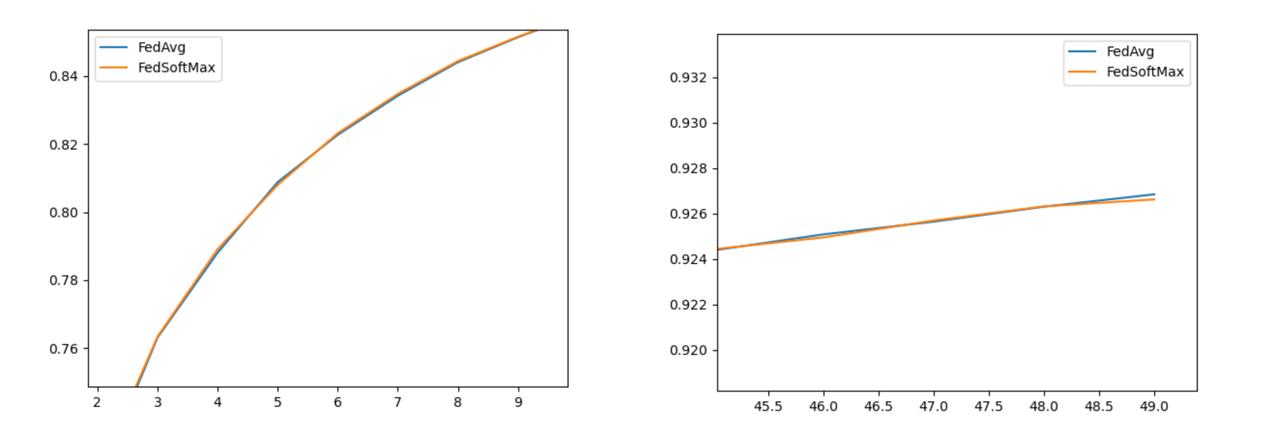
Figure 2: Comparative analysis between FedAvg and FedSoftMax: Final and intermediate accuracy in IID framwork.
The horizontal axis accounts for communication round and the vertical axes accounts for the accuracy reached. These results are the ones obtained on MNIST.

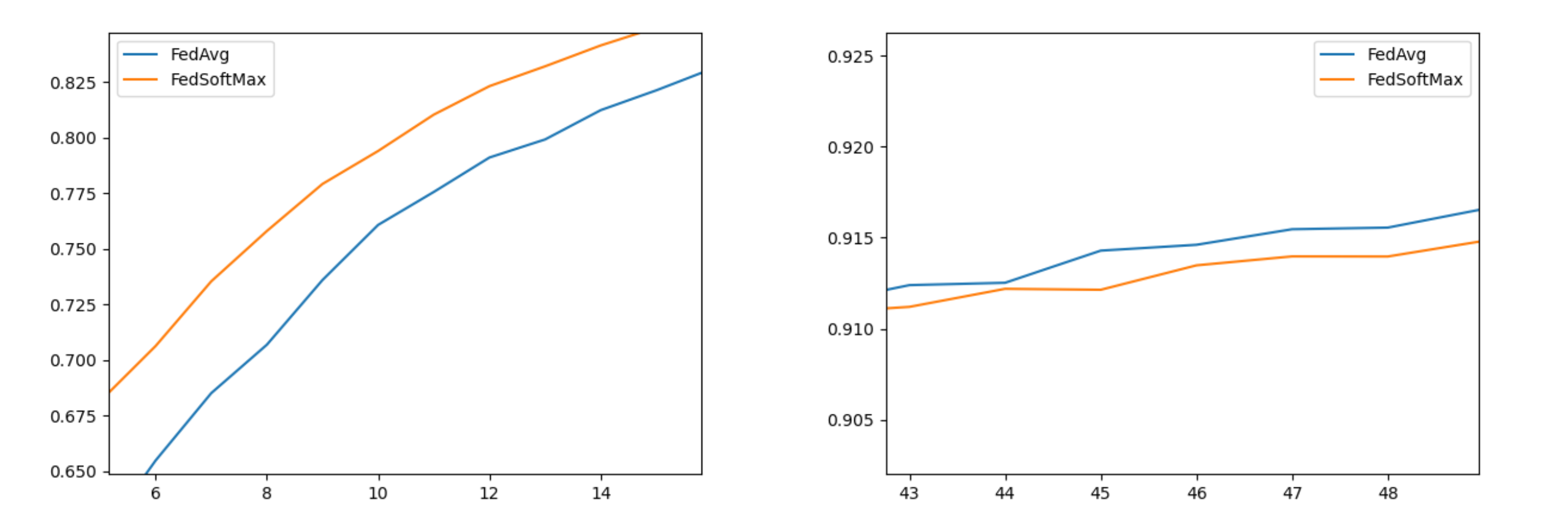
Figure 3: Comparative analysis between FedAvg and FedSoftMax: Final and intermediate accuracy in not IID framework.
The horizontal axis accounts for communication round and the vertical axes accounts for the accuracy reached. These results are the ones obtained on MNIST.

Figure 4: Comparative analysis between FedAvg and FedSoftMax.
The horizontal axis accounts for communication round and the vertical axes accounts for the accuracy reached. The image bottom left refers to the IID framework, the top left to the not IID framework and the right one to the extremely not-IID framework. These results are the ones obtained on MNIST.

Table 3: Results concerning convergence speed ($R_{90}$).

Framework	Algorithm	Confidence Interval for $R_{90}$
TNIID	FedAvg	14.877887807248147 - 15.842112192751852
TNIID	FedSoftMax	7.855914695373678 - 8.704085304626322
NIID	FedAvg	12.726276322973177 - 13.957934203342614
NIID	FedSoftMax	9.996249956446318 - 11.31953951723789
IID	FedAvg	21.527442685457743 - 24.58366842565337
IID	FedSoftMax	21.607110478485172 - 24.504000632625942

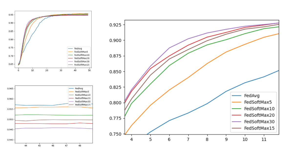
Figure 5: Comparative analysis between FedAvg and FedSoftMax(T) for several values of T, the temperature.
The horizontal axis accounts for communication round and the vertical axes accounts for the accuracy reached. These results are the ones obtained on MNIST in not IID framework.

Weakness and Strength of the Strategies Proposed

One potential weakness that has emerged from the theory is that the method potentially converges to a different value of the optimum. We were therefore interested in studying whether experimentally a significant difference could be observed and whether this might preclude the use of the method. With this purpose, we studied the evolution of $\alpha_{i}$. The result is extremely positive, not only do we see that the imbalance produced is minimal, but rather we observe that the $\alpha_{i}$ almost always converges to the $p_{i}$ with a rate of $1/t$ (see Figure 6). All these entails the following remark:

Remark 10

FedSoftMax is natural smooth interpolation between FedAvg and FedMax($k$), taking the advantage from the higher convergence speed of FedMax($k$) in the initial phase and the stability and correctness of FedAvg in the rest of the learning.

In fact FedMax(k) methods, while speeding the process at the beginning, give poor results when it comes to the final accuracy. This can actually be well visualized by analyzing the top losses of clients during FedSoftMax running (see Figure 7). We actually see that only a small group of clients are used through all the process, and while this is profitable for speed purposes in the first rounds, it has a huge drawback in the following rounds since we only use a small amount of data that (by non-IIDness) is not representative of the whole dataset. There lies the power of FedSoftMax, which enables to use both the speed-up ability of FedMax, and the data of all clients at the end as in FedAvg.

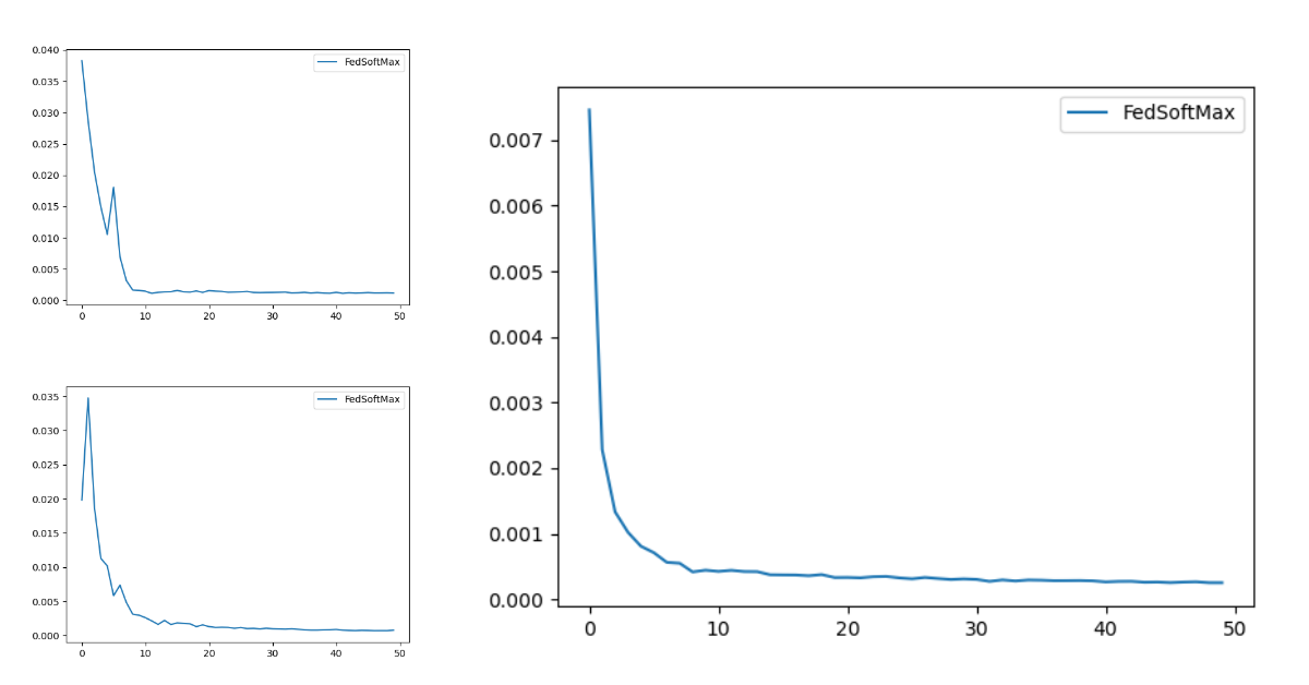
Figure 6: Convergence of $\alpha_{i}$ to $p_{i}$ as a function of time (represented through the communication rounds) in the IID framework.
The horizontal axis accounts for communication round and the vertical axes accounts for the difference among $\alpha_{i}$ and $p_{i}$. These results are the ones obtained on MNIST.

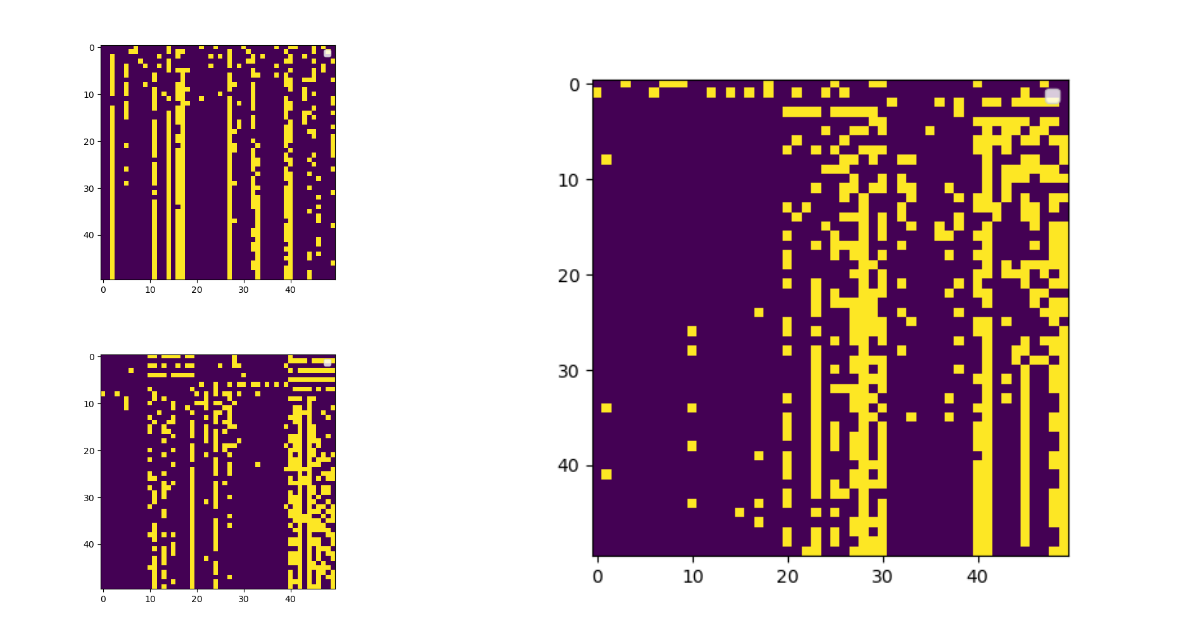
Figure 7: Clients participation in the aggregation process
The horizontal axis accounts for a unique identifier of the client and the vertical axis accounts for the communication round. The value of the $\alpha_{i}$ is encoded through colors. Then ten highest values are colored in yellow, while the others are colored in blue. These results are the one obtained on MNIST.

Finally, we became interested in measuring the stability of FedSoftMax when compared to FedAvg. For this purpose we use a lag one autocorrelation measure based on the normalized standard deviation of the variations over one round. The results in this case show a more pronounced tendency toward instability than FedSoftMax, which nevertheless appears to be reasonably stable (see Table 4).

Table 4: Results concerning stability.

Framework	Algorithm	Smoothness value
TNIID	FedAvg	1.3686297084899968
TNIID	FedSoftMax	2.322656907880106
NIID	FedAvg	1.3404421487057407
NIID	FedSoftMax	1.7307167213190393
IID	FedAvg	2.8107170960158876
IID	FedSoftMax	2.7724249879251603

3.3 Discussion & Final Remarks

We have extended the insightful analysis already carried out by Cho et al. (2022b), and examined further the joint evolution of $\overline{\rho}$ and $\tilde{\rho}$, obtaining simpler bounds. Taking advantage of these theoretical insights, we have proposed a family of aggregation strategies, among which FedSoftMax is the most relevant one. Here, we complement our previous work by investigating empirically the latter with the goal of finding out weaknesses and of quantifying its strength for potential exploitation in practice. The experimental results fully confirm the theory and also suggest that the bias introduced by mismatched weighting of the data distribution does not affect the quality of the final results. Moreover, this method seems to naturally converge to FedAvg leveraging the biases introduced in the first communication rounds.

Further directions of research

Several aspects emerged may be object of further analysis. We report them as associated research questions. From a theoretical point of view, we propose 3 possible directions to investigate:
Proposed Research Question 1 Is it possible to obtain expressive bounds weakening at least one of the 4 assumptions introduced? We believe interesting results could be obtained by weakening of assumption 3.

Proposed Research Question 2 Can we substitute the learning algorithm used throughout all the analysis, i.e. SGD mini-batch, with others? We believe that interesting results may come even using fairly natural algorithms such as GD.

Proposed Research Question 3 The experiments have shown that the $\alpha_{i}$ coefficients converge to the $p_{i}$ in a framework where datasets are not too much non-IID. We might thus be interested in both proving this affirmation under supplementary hypothesis, and to see its consequences when it comes to the adaptation of the main theorem.

Moreover, we actually see that in the case of a very non-IID dataset the $\alpha_{i}$ actually do not converge to the $p_{i}$, but they still converge to some fixed limits, and it would be interested to study these limits, and their potential correlation with the $F_{i}^{*}$ or other client dependent parameters.

Proposed Research Question 4 Figure 5 showed the correlation between parameter $T$ of the FedSoftMax method and the gain in speed. Further experiments not shown here show that increasing further $T^{-1}$ increases the speed up to a certain limits, i.e. the accuracy curves tend to converge to a ”maximal-speed” curve. Not only could we empirically study the properties of this limit curve, but we could also try to give theoretical evidence for this observation.

Proposed Research Question 5 Can we extend our results to the non-convex setting? We suggest to start introducing some simplifying conditions such as the ones associated to the Polyak-Łojasiewicz inequality.
From a practical point of view, it could be interesting to investigate if there is a practical advantage induced by the speed-up given by FedSoftMax.

Acknowledgements

This work was granted access to HPC resources of MesoPSL financed by the Region Ile de France and the project Equip@Meso (reference ANR-10-EQPX-29-01) of the programme Investissements d’Avenir supervised by the Agence Nationale pour la Recherche.

Appendix A Proof of the Main Theorem & its Corollary

Proof (Main Theorem) The first step of the proof consists in rewriting the argument of the expectation at the LHS of Inequality 3. In particular, we apply the definition of $w_{t+1}$, add and subtract the same quantity, and eventually develop the square. This leads to the following expression.

$$\left\lVert w_{t+1}-w^{\star}\right\rVert^{2} =\left\lVert w_{t}-w^{\star}\right\rVert^{2}-2\eta_{t}\left\langle w_{t}-w^{\star},\sum\limits_{i\in I}\alpha_{t}^{i}\nabla F_{i}(w_{t}^{i})\right\rangle$$

$$+2\eta_{t}\left\langle w_{t}-w^{\star}-\eta_{t}\sum\limits_{i\in I}\alpha_{t}^{i}\nabla F_{i}(w_{t}^{i}),\sum\limits_{i\in I}\alpha_{t}^{i}\nabla F_{i}(w_{t}^{i})-\sum\limits_{i\in I}\alpha_{t}^{i}g_{i}(w_{t}^{i})\right\rangle$$

$$+\left\lVert\eta_{t}\sum\limits_{i\in I}\alpha_{t}^{i}\nabla F_{i}(w_{t}^{i})\right\rVert^{2}+\eta_{t}^{2}\left\lVert\sum\limits_{i\in I}\alpha_{t}^{i}\nabla F_{i}(w_{t}^{i})-\sum\limits_{i\in I}\alpha_{t}^{i}g_{i}(w_{t}^{i})\right\rVert^{2}$$

For seek of simplicity, we denote the addends at the RHS, as follows:

$$=\left\lVert w_{t}-w^{\star}\right\rVert^{2}+A_{1}+A_{2}+A_{3}+A_{4}$$

The rest of the proof consists in bounding, sequentially, each of these addends.
Concerning term $A_{1}$, we apply Cauchy-Schwartz inequality and by exploiting the convexity of the functions involved. Then, we derive the consequences of Assumption 1 and take advantage from the fact that $\nabla F_{i}(w_{i}^{\star})=0$. This leads to the following upper bound for $A_{1}$:

$$\leq\sum\limits_{i\in I}\alpha_{t}^{i}\left\lVert w_{t}-w_{t}^{i}\right\rVert^{2}+2L\eta_{t}^{2}\sum\limits_{i\in I}\alpha_{t}^{i}(F_{i}(w_{t}^{i})-F_{i}^{\star})-2\eta_{t}\sum\limits_{i\in I}\alpha_{t}^{i}\left\langle w_{t}^{i}-w^{\star},\nabla F_{i}(w_{t}^{i})\right\rangle$$

then, by using Assumption 2, we can rewrite the last term of the previous inequality and applying Lemma 1, we obtain the final upper bound for $A_{1}$. These steps are reported below:

$$A_{1} \leq-2\eta_{t}\sum\limits_{i\in I}\alpha_{t}^{i}(F_{i}(w_{t}^{i})-F_{i}(w^{\star})+\frac{\mu}{2}\left\lVert w_{t}^{i}-w^{\star}\right\rVert^{2})$$

$$\leq\eta_{t}^{2}E^{2}G^{2}-\eta_{t}\mu\sum\limits_{i\in I}\alpha_{t}^{i}\left\lVert w_{t}^{i}-w^{\star}\right\rVert^{2}+2L\eta_{t}^{2}\sum\limits_{i\in I}\alpha_{t}^{i}(F_{i}(w_{t}^{i})-F_{i}^{\star})$$

$$-2\eta_{t}\sum\limits_{i\in I}\alpha_{t}^{i}(F_{i}(w_{t}^{i})-F_{i}(w^{\star}))$$

For bounding term $A_{2}$, we observe that, for the unbiasedness of the gradient estimator, $\mathds{E}(A_{2})=0$. The bound for $A_{3}$ requires exclusively the application of Assumption 1:

$$A_{3} =\left\lVert\eta_{t}\sum\limits_{i\in I}\alpha_{t}^{i}\nabla F_{i}(w_{t}^{i})\right\rVert^{2}\leq 2L\eta_{t}^{2}\sum\limits_{i\in I}\alpha_{t}^{i}(F_{i}(w_{t}^{i})-F_{i}^{\star})$$

Then, we obtain the bound for $A_{4}$ by applying Jensen’s inequality, exploiting the linearity of the expected value and using Assumption 3.

$$A_{4} \leq\eta_{t}^{2}\sum\limits_{i\in I}\alpha_{t}^{i}\sigma^{2}\leq\eta_{t}^{2}\sigma^{2}$$

This sequence of bounds allows us to write the following expression:

$$\mathbb{E}[\left\lVert w_{t+1}-w^{\star}\right\rVert^{2}]\leq (1-\eta_{t}\mu)\mathbb{E}[\left\lVert w_{t}-w^{\star}\right\rVert^{2}]+16\eta_{t}^{2}E^{2}G^{2}+\eta_{t}^{2}\sigma^{2}$$

$$\quad+4L\eta_{t}^{2}\mathbb{E}[\sum\limits_{i\in I}\alpha_{t}^{i}(F_{i}(w_{t}^{i})-F_{i}^{\star})]$$

$$-2\eta_{t}\mathbb{E}[\sum\limits_{i\in I}\alpha_{t}^{i}(F_{i}(w_{t}^{i})-F_{i}(w^{\star}))]$$

Renaming the latter terms, we have that:

$$=(1-\eta_{t}\mu)\mathbb{E}[\left\lVert w_{t}-w^{\star}\right\rVert^{2}]+16\eta_{t}^{2}E^{2}G^{2}+\eta_{t}^{2}\sigma^{2}+A_{5}$$

Bounding $A_{5}$, it’s slightly more complicated, but the sequence of operations required is fairly similar to the one done above. The final upper bound is the following:

$$A_{5} \leq\eta_{t}^{2}(16E^{2}G^{2}+6\overline{\rho}L\Gamma)-\frac{3}{8}\eta_{t}\mu\overline{\rho}\mathbb{E}[\left\lVert w_{t}-w^{\star}\right\rVert^{2}]+2\eta_{t}\Gamma(\tilde{\rho}-\overline{\rho})$$

The proof is completed as follows:

$$\left\lVert w_{t+1}-w^{\star}\right\rVert^{2} \leq(1-\eta_{t}\mu)\mathbb{E}[\left\lVert w_{t}-w^{\star}\right\rVert^{2}]+16\eta_{t}^{2}E^{2}G^{2}+\eta_{t}^{2}\sigma^{2}+A_{5}$$

$$\leq(1-\eta_{t}\mu(1+\frac{3}{8}\overline{\rho}))\mathbb{E}[\left\lVert w_{t}-w^{\star}\right\rVert^{2}]+\eta_{t}^{2}(32E^{2}G^{2}+6\overline{\rho}L\Gamma+\sigma^{2})$$

$$+2\eta_{t}\Gamma(\tilde{\rho}-\overline{\rho})$$

Proof (Corollary) The proof is fairly simple and brief. We start rewriting the main Theorem, as follows:

$$\Delta_{t+1}\leq(1-\eta_{t}\mu B)\Delta_{t}+\eta_{t}^{2}C+\eta_{t}D$$

where:

$B=(1+\frac{3}{8}\overline{\rho})$, $C=32E^{2}G^{2}+6\overline{\rho}L\Gamma+\sigma^{2}$, and $D=2\Gamma(\tilde{\rho}-\overline{\rho})$

Let $\psi$ be the $\max\left\{\gamma\left\lVert w_{0}-w^{\star}\right\rVert^{2},\frac{1}{\beta\mu B-1}\left(\beta^{2}C+D\beta(t+\gamma)\right)\right\}$, where $\beta>\frac{1}{\mu B}$, $\gamma>0$.
The proof proceed by induction; from this argument, we derive that:

$$\forall t,\Delta_{t}\leq\frac{\psi}{t+\gamma}$$

Then, by the L-smoothness of $F$, we obtain the following upper bound that concludes the proof.

$$\mathbb{E}\left[F\left(w_{t}\right)\right]-F^{\star}\leq\frac{L}{2}\Delta_{t}\leq\frac{L}{2}\frac{\psi}{\gamma+t}$$

References

- Bagdasaryan et al. (2020) Eugene Bagdasaryan, Andreas Veit, Yiqing Hua, Deborah Estrin, and Vitaly Shmatikov. How to backdoor federated learning. In International Conference on Artificial Intelligence and Statistics, pages 2938–2948. PMLR, 2020.
- Berahas et al. (2022) Albert S Berahas, Frank E Curtis, and Baoyu Zhou. Limited-memory bfgs with displacement aggregation. Mathematical Programming, 194(1-2):121–157, 2022.
- Bergou et al. (2022) El Houcine Bergou, Konstantin Burlachenko, Aritra Dutta, and Peter Richtárik. Personalized federated learning with communication compression. arXiv preprint arXiv:2209.05148, 2022.
- Bonawitz et al. (2019) Keith Bonawitz, Fariborz Salehi, Jakub Konečnỳ, Brendan McMahan, and Marco Gruteser. Federated learning with autotuned communication-efficient secure aggregation. In 2019 53rd Asilomar Conference on Signals, Systems, and Computers, pages 1222–1226. IEEE, 2019.
- Charles et al. (2022) Zachary Charles, Kallista Bonawitz, Stanislav Chiknavaryan, Brendan McMahan, et al. Federated select: A primitive for communication-and memory-efficient federated learning. arXiv preprint arXiv:2208.09432, 2022.
- Chen et al. (2018) Fei Chen, Mi Luo, Zhenhua Dong, Zhenguo Li, and Xiuqiang He. Federated meta-learning with fast convergence and efficient communication. arXiv preprint arXiv:1802.07876, 2018.
- Chen et al. (2017) Wenlin Chen, Samuel Horvath, and Peter Richtarik. Optimal client sampling for federated learning. Transactions on Machine Learning Research, 2017.
- Chen et al. (2019) Yang Chen, Xiaoyan Sun, and Yaochu Jin. Communication-efficient federated deep learning with layerwise asynchronous model update and temporally weighted aggregation. IEEE transactions on neural networks and learning systems, 31(10):4229–4238, 2019.
- Cho et al. (2020) Yae Jee Cho, Jianyu Wang, and Gauri Joshi. Client selection in federated learning: Convergence analysis and power-of-choice selection strategies. arXiv preprint arXiv:2010.01243, 2020.
- Cho et al. (2021) Yae Jee Cho, Jianyu Wang, Tarun Chiruvolu, and Gauri Joshi. Personalized federated learning for heterogeneous clients with clustered knowledge transfer. arXiv preprint arXiv:2109.08119, 2021.
- Cho et al. (2022a) Yae Jee Cho, Andre Manoel, Gauri Joshi, Robert Sim, and Dimitrios Dimitriadis. Heterogeneous ensemble knowledge transfer for training large models in federated learning. arXiv preprint arXiv:2204.12703, 2022a.
- Cho et al. (2022b) Yae Jee Cho, Jianyu Wang, and Gauri Joshi. Towards understanding biased client selection in federated learning. In International Conference on Artificial Intelligence and Statistics, pages 10351–10375. PMLR, 2022b.
- Corinzia et al. (2019) Luca Corinzia, Ami Beuret, and Joachim M Buhmann. Variational federated multi-task learning. arXiv preprint arXiv:1906.06268, 2019.
- Dai et al. (2015) Wei Dai, Abhimanu Kumar, Jinliang Wei, Qirong Ho, Garth Gibson, and Eric Xing. High-performance distributed ml at scale through parameter server consistency models. In Proceedings of the AAAI Conference on Artificial Intelligence, volume 29, 2015.
- Deng (2012) Li Deng. The mnist database of handwritten digit images for machine learning research [best of the web]. IEEE signal processing magazine, 29(6):141–142, 2012.
- Duchi et al. (2013) John Duchi, Michael I Jordan, and Brendan McMahan. Estimation, optimization, and parallelism when data is sparse. Advances in Neural Information Processing Systems, 26, 2013.
- Eichner et al. (2019) Hubert Eichner, Tomer Koren, Brendan McMahan, Nathan Srebro, and Kunal Talwar. Semi-cyclic stochastic gradient descent. In International Conference on Machine Learning, pages 1764–1773. PMLR, 2019.
- Gower et al. (2019) Robert Mansel Gower, Nicolas Loizou, Xun Qian, Alibek Sailanbayev, Egor Shulgin, and Peter Richtárik. Sgd: General analysis and improved rates. In International conference on machine learning, pages 5200–5209. PMLR, 2019.
- Horváth et al. (2022) Samuel Horváth, Maziar Sanjabi, Lin Xiao, Peter Richtárik, and Michael Rabbat. Fedshuffle: Recipes for better use of local work in federated learning. arXiv preprint arXiv:2204.13169, 2022.
- Huang et al. (2022) Tiansheng Huang, Weiwei Lin, Li Shen, Keqin Li, and Albert Y Zomaya. Stochastic client selection for federated learning with volatile clients. IEEE Internet of Things Journal, 9(20):20055–20070, 2022.
- Jhunjhunwala et al. (2022) Divyansh Jhunjhunwala, Pranay Sharma, Aushim Nagarkatti, and Gauri Joshi. Fedvarp: Tackling the variance due to partial client participation in federated learning. In Uncertainty in Artificial Intelligence, pages 906–916. PMLR, 2022.
- Jiang and Agrawal (2018) Peng Jiang and Gagan Agrawal. A linear speedup analysis of distributed deep learning with sparse and quantized communication. Advances in Neural Information Processing Systems, 31, 2018.
- Jin et al. (2022) Jiayin Jin, Jiaxiang Ren, Yang Zhou, Lingjuan Lyu, Ji Liu, and Dejing Dou. Accelerated federated learning with decoupled adaptive optimization. In International Conference on Machine Learning, pages 10298–10322. PMLR, 2022.
- Karimireddy et al. (2022) Sai Praneeth Karimireddy, Wenshuo Guo, and Michael I Jordan. Mechanisms that incentivize data sharing in federated learning. arXiv preprint arXiv:2207.04557, 2022.
- Khodak et al. (2019) Mikhail Khodak, Maria-Florina F Balcan, and Ameet S Talwalkar. Adaptive gradient-based meta-learning methods. Advances in Neural Information Processing Systems, 32, 2019.
- Konečnỳ et al. (2016) Jakub Konečnỳ, H Brendan McMahan, Felix X Yu, Peter Richtárik, Ananda Theertha Suresh, and Dave Bacon. Federated learning: Strategies for improving communication efficiency. arXiv preprint arXiv:1610.05492, 2016.
- Li et al. (2019) Tian Li, Maziar Sanjabi, Ahmad Beirami, and Virginia Smith. Fair resource allocation in federated learning. arXiv preprint arXiv:1905.10497, 2019.
- Li et al. (2020a) Tian Li, Anit Kumar Sahu, Ameet Talwalkar, and Virginia Smith. Federated learning: Challenges, methods, and future directions. IEEE signal processing magazine, 37(3):50–60, 2020a.
- Li et al. (2020b) Tian Li, Anit Kumar Sahu, Ameet Talwalkar, and Virginia Smith. Federated learning: Challenges, methods, and future directions. IEEE signal processing magazine, 37(3):50–60, 2020b.
- Lim et al. (2020) Wei Yang Bryan Lim, Nguyen Cong Luong, Dinh Thai Hoang, Yutao Jiao, Ying-Chang Liang, Qiang Yang, Dusit Niyato, and Chunyan Miao. Federated learning in mobile edge networks: A comprehensive survey. IEEE Communications Surveys & Tutorials, 22(3):2031–2063, 2020.
- Liu et al. (2020) Wei Liu, Li Chen, Yunfei Chen, and Wenyi Zhang. Accelerating federated learning via momentum gradient descent. IEEE Transactions on Parallel and Distributed Systems, 31(8):1754–1766, 2020.
- McMahan et al. (2017a) Brendan McMahan, Eider Moore, Daniel Ramage, Seth Hampson, and Blaise Aguera y Arcas. Communication-efficient learning of deep networks from decentralized data. In Artificial intelligence and statistics, pages 1273–1282. PMLR, 2017a.
- McMahan et al. (2017b) Brendan McMahan, Eider Moore, Daniel Ramage, Seth Hampson, and Blaise Aguera y Arcas. Communication-efficient learning of deep networks from decentralized data. In Artificial intelligence and statistics, pages 1273–1282. PMLR, 2017b.
- Mendieta et al. (2022) Matias Mendieta, Taojiannan Yang, Pu Wang, Minwoo Lee, Zhengming Ding, and Chen Chen. Local learning matters: Rethinking data heterogeneity in federated learning. In Proceedings of the IEEE/CVF Conference on Computer Vision and Pattern Recognition, pages 8397–8406, 2022.
- Mohri et al. (2019) Mehryar Mohri, Gary Sivek, and Ananda Theertha Suresh. Agnostic federated learning. In International Conference on Machine Learning, pages 4615–4625. PMLR, 2019.
- Nishio and Yonetani (2019) Takayuki Nishio and Ryo Yonetani. Client selection for federated learning with heterogeneous resources in mobile edge. In ICC 2019-2019 IEEE international conference on communications (ICC), pages 1–7. IEEE, 2019.
- Reddi et al. (2020) Sashank Reddi, Zachary Charles, Manzil Zaheer, Zachary Garrett, Keith Rush, Jakub Konečnỳ, Sanjiv Kumar, and H Brendan McMahan. Adaptive federated optimization. arXiv preprint arXiv:2003.00295, 2020.
- Sannara et al. (2021) EK Sannara, Francois Portet, Philippe Lalanda, and VEGA German. A federated learning aggregation algorithm for pervasive computing: Evaluation and comparison. In 2021 IEEE International Conference on Pervasive Computing and Communications (PerCom), pages 1–10. IEEE, 2021.
- Shang et al. (2022) Xinyi Shang, Yang Lu, Gang Huang, and Hanzi Wang. Federated learning on heterogeneous and long-tailed data via classifier re-training with federated features. IJCAI-ECAI 2022, 2022.
- Tan et al. (2022) Alysa Ziying Tan, Han Yu, Lizhen Cui, and Qiang Yang. Towards personalized federated learning. IEEE Transactions on Neural Networks and Learning Systems, 2022.
- Wang et al. (2020) Jianyu Wang, Qinghua Liu, Hao Liang, Gauri Joshi, and H Vincent Poor. Tackling the objective inconsistency problem in heterogeneous federated optimization. Advances in neural information processing systems, 33:7611–7623, 2020.
- Xiao et al. (2017) Han Xiao, Kashif Rasul, and Roland Vollgraf. Fashion-mnist: a novel image dataset for benchmarking machine learning algorithms. arXiv preprint arXiv:1708.07747, 2017.
- Yang et al. (2021) Chengxu Yang, Qipeng Wang, Mengwei Xu, Zhenpeng Chen, Kaigui Bian, Yunxin Liu, and Xuanzhe Liu. Characterizing impacts of heterogeneity in federated learning upon large-scale smartphone data, 2021.
- Yurochkin et al. (2019) Mikhail Yurochkin, Mayank Agarwal, Soumya Ghosh, Kristjan Greenewald, Nghia Hoang, and Yasaman Khazaeni. Bayesian nonparametric federated learning of neural networks. In International conference on machine learning, pages 7252–7261. PMLR, 2019.
- Zhao et al. (2021) Haoyu Zhao, Zhize Li, and Peter Richtárik. Fedpage: A fast local stochastic gradient method for communication-efficient federated learning. arXiv preprint arXiv:2108.04755, 2021.
- Zheng et al. (2019) Yandong Zheng, Rongxing Lu, Beibei Li, Jun Shao, Haomiao Yang, and Kim-Kwang Raymond Choo. Efficient privacy-preserving data merging and skyline computation over multi-source encrypted data. Information Sciences, 498:91–105, 2019.
- (47) Hanhan Zhou, Tian Lan, Guru Prasadh Venkataramani, and Wenbo Ding. Federated learning with online adaptive heterogeneous local models. In Workshop on Federated Learning: Recent Advances and New Challenges (in Conjunction with NeurIPS 2022).
- Zhou et al. (2022) Hanhan Zhou, Tian Lan, Guru Venkataramani, and Wenbo Ding. On the convergence of heterogeneous federated learning with arbitrary adaptive online model pruning. arXiv preprint arXiv:2201.11803, 2022.