Contract-Based Distributed Synthesis in Two-Objective Parity Games

Abstract

We present a novel method to compute assume-guarantee contracts in non-zerosum two-player games over finite graphs where each player has a different $\omega$-regular winning condition. Given a game graph $G$ and two parity winning conditions $\Phi_{0}$ and $\Phi_{1}$ over $G$, we compute contracted strategy-masks (csm) $(\Psi_{i},\Pi_{i})$ for each $\text{Player}\leavevmode\nobreak\ i$. Within a csm, $\Pi_{i}$ is a permissive strategy template which collects an infinite number of winning strategies for $\text{Player}\leavevmode\nobreak\ i$ under the assumption that $\text{Player}\leavevmode\nobreak\ 1-i$ chooses any strategy from the permissive assumption template $\Psi_{i}$. The main feature of csm’s is their power to fully decentralize all remaining strategy choices – if the two player’s csm’s are compatible, they provide a pair of new local specifications $\Phi_{0}^{\bullet}$ and $\Phi_{1}^{\bullet}$ such that $\text{Player}\leavevmode\nobreak\ i$ can locally and fully independently choose any strategy satisfying $\Phi_{i}^{\bullet}$ and the resulting strategy profile is ensured to be winning in the original two-objective game $(G,\Phi_{0},\Phi_{1})$. In addition, the new specifications $\Phi_{i}^{\bullet}$ are maximally cooperative, i.e., allow for the distributed synthesis of any cooperative solution. Further, our algorithmic computation of csm’s is complete and ensured to terminate.

We illustrate how the unique features of our synthesis framework effectively address multiple challenges in the context of “correct-by-design” logical control software synthesis for cyber-physical systems and provide empirical evidence that our approach possess desirable structural and computational properties compared to state-of-the-art techniques.

1 Introduction

Games on graphs provide an effective way to formalize synthesis problems in the context of correct-by-construction cyber-physical systems (CPS) design. A prime example are algorithms to synthesize control software that ensures the satisfaction of logical specifications under the presence of an external environment, which e.g., causes changed task assignments, transient operating conditions, or unavoidable interactions with other system components. The resulting logical control software typically forms a higher layer of the control software stack. The details of the underlying physical dynamics and actuations are then abstracted away into the structure of the game graph utilized for synthesis [38, 2].

Algorithmically, the outlined control design procedure via games-on-graphs utilizes reactive synthesis [25, 30], a well understood and highly automated design flow originating from the formal methods community rooted in computer science. The strength of utilizing reactive synthesis for logical control design is its ability to provide strong correctness guarantees by treating the environment as fully adversarial. While this view is useful if a single controller is designed for a system which needs to obey the specification in an unknown environment, it does not excel at synthesizing distributed and interacting logical control software for large-scale CPS. In this context, each component acts as the “environment” for another one and controllers for components are designed concurrently. Here, if known a-priory, the control design of one component could take the needs of other components into account and does not need to be treated fully adversarial.

Within this paper, we approach this problem by modelling a distributed logical control synthesis problem with two components as a non-zerosum two-player game over a finite graph $G$ where each player models one component and has its own parity winning condition $\Phi_{0}$ and $\Phi_{1}$ over $G$. Given such a two-objective parity game $(G,\Phi_{0},\Phi_{1})$, we develop a new distributed synthesis method which utilizes assume-guarantee contracts to formalize the needs for cooperation between components (i.e. players). Assume-guarantee reasoning has proven to be very useful in the context of distributed program verification [34, 37, 31, 1]. Here, all component implementations are known and therefore allow to extract contracts which are utilized to check their correctness locally. In distributed synthesis, however, one encounters a chicken-and-egg problem – without existing implementations, no contracts can be extracted and without contracts, no respecting implementations can be synthesized. Due to this difficulty, efficient techniques for assume-guarantee distributed synthesis are mostly missing.

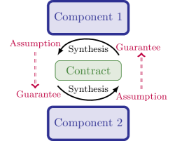
Figure 1: Schematic representation of the negotiation framework.

In order to close this gap, this paper develops a novel decentralized iterative negotiation framework which co-designs contracts and implementations via iterative contract refinements (see Fig. 1 for a schematic representation). This iterative refinement is enabled by a novel formalization of contracted strategy-masks (csm) $(\Psi_{i},\Pi_{i})$ for each $\text{Player}\leavevmode\nobreak\ i$ which encodes the essence of the required cooperation between players in a concise data structure. Contracted strategy-masks are based on the idea of permissive templates which were recently introduced to formalize and synthesize permissive assumptions [4] and permissive strategies [6] in (zero-sum) parity games. Within a csm, $\Pi_{i}$ is a strategy template which collects an infinite number of winning strategies for $\text{Player}\leavevmode\nobreak\ i$ under the assumption that $\text{Player}\leavevmode\nobreak\ 1-i$ chooses any strategy from the assumption template $\Psi_{i}$. While the known efficient computability, adaptability, and compositionality of permissive templates enables us to achieve an efficient, surely terminating algorithm for csm computation, the novel feature of csm’s is their power to fully decentralize all remaining strategy choices – if the two player’s csm’s encode a compatible contract, each player can locally and fully independently choose any strategy contained in $\Pi_{i}$ and the resulting strategy profile is ensured to be winning in the original two-objective game $(G,\Phi_{0},\Phi_{1})$. In addition, our algorithmic computation of csm’s is both distributed and complete – i.e., iff the original two-objective game $(G,\Phi_{0},\Phi_{1})$ is realizable, compatible csm’s are always returned by our negotiation framework, despite the fact that most computations are done distributed in each component. To the best of our knowledge, this is the first contract-based distributed synthesis framework for the full class of $\omega$-regular specifications with these capabilities.

To show the practical importance of our new technique, we utilize our synthesis framework to efficiently tackle three relevant problems arising from applications of two-player games in the context of cyber-physical system design – (i) distributed (privacy preserving) synthesis, i.e., local synthesis of coupled mission controllers with limited shared specification and strategy information, (ii) incremental synthesis and negotiation, i.e., adapting strategies to newly arriving, additional $\omega$-regular objectives $\Phi_{i}^{\prime}$, and (ii) fault-tolerant strategy adaptation, i.e., online adaptation of local controllers to the occasional or persistent unavailability of actuators.

Related Work.

In the field of reactive synthesis, there are several approaches to synthesize strategies for non-zerosum two-player games. In [12], even though the setting is non-zerosum, the authors considered the players to be antagonistic. In particular, their work relies on secure equilibria [13], a refinement of Nash equilibria [32], where players first try to satisfy their own specification, and then try to falsify the specification of the other player. So, the algorithm given by the authors computes a secure-equilibirum strategy profile. Similarly, in [19], the authors search for a strategy profile that is an equilibiria in the sense that the players have no incentive to deviate from their strategies. In [9, 15, 18], the authors do not fix such a strategy profile for the players, but they assume a particular rational behavior for the players, formalized as dominant or admissible strategies. This leads to implicit assumptions on other players behavior which can be exploited for local realizability. In contrast, our work computes explicit assumptions and hence, gives players the freedom to choose any strategy that satisfies imposed assumptions without requiring any particularly rational strategy choice.

Similar to our approach, [17, 27, 26] also compute an explicit contract between components, and then each component can choose any strategy that respects the contract. While [17] uses a single centralized bounded synthesis problem to find contracts between multiple interacting components, the approaches in [27] and [26] employ a negotiation algorithm between two local synthesis problems, and are, therefore conceptually more similar to ours. However, the problem tackled in [26] comes from the area of supervisory control and therefore uses a different formulation of component interaction. The work closest to ours is [27], which constructs assumptions using the work of [11], which are, however not maximally cooperative. We discuss the unique features of our approach compared to [17, 27] for the application to CPS synthesis problems again in Section 7, where we also provide a limited empirical comparison.

Outline.

This paper consists of two parts. First, in Section 2-6, we develop the theory behind our new negotiation framework, derive the algorithms to solve it and prove their correctness. Second, in Section 7, we show how two-objective parity games arise in the synthesis of logical control software for CPS and formalize the additional features of our synthesis framework in this application domain. We further provide empirical evidence that our negotiation framework also possess desirable computational properties.

For readers looking for additional motivation of the considered synthesis problem, we recommend reading Section 7.1 before moving on to Section 2.

2 Preliminaries

Notations

We use $\mathbb{N}$ to denote the set of natural numbers including zero. Given two natural numbers $a,b\in\mathbb{N}$ with $a<b$, we use $[a;b]$ to denote the set $\left\{n\in\mathbb{N}\mid a\leq n\leq b\right\}$.

Let $\Sigma$ be a finite alphabet. The notations $\Sigma^{*}$ and $\Sigma^{\omega}$ respectively denote the set of finite and infinite words over $\Sigma$. Given two words $u\in\Sigma^{*}$ and $v\in\Sigma^{*}\cup\Sigma^{\omega}$, the concatenation of $u$ and $v$ is written as the word $uv$.

Game Graphs

A game graph is a tuple $G=\left(V=V^{0}\mathbin{\mathaccent 0{\cdot}\cup}V^{1},E\right)$ where $(V,E)$ is a finite directed graph with vertices $V$ and edges $E$, and $V_{0},V_{1}\subseteq V$ form a partition of $V$. Without loss of generality, we assume that for every $v\in V$ there exists $v^{\prime}\in V$ s.t. $(v,v^{\prime})\in E$. A play originating at a vertex $v_{0}$ is an infinite sequence of vertices $\rho=v_{0}v_{1}\ldots\in V^{\omega}$.

Winning Conditions

Given a game graph $G$, a winning condition (or objective) is a set of plays specified using a formula $\Phi$ in linear temporal logic (LTL) over the vertex set $V$. That is, we consider LTL formulas whose atomic propositions are sets of vertices from $V$. In this case the set of desired infinite plays is given by the semantics of $\Phi$ which is an $\omega$-regular language $\mathcal{L}(G,\Phi)\subseteq V^{\omega}$. When clear from the context, we will drop the mention of game graph $G$, and simply write $\mathcal{L}(\Phi)$ instead. Every game graph with an arbitrary $\omega$-regular set of desired plays can be reduced to a game graph (possibly with a different set of vertices) with a LTL winning condition. The standard definitions of $\omega$-regular languages and LTL are omitted for brevity and can be found in standard textbooks [7].

Games

A two-players (turn-based) game is a tuple $\mathcal{G}=\left(G,\Phi\right)$, where $G$ is a game graph, and $\Phi$ is the winning condition over $G$. A two-players (turn-based) two-objectives game is a triple $\mathcal{G}=\left(G,\Phi_{0},\Phi_{1}\right)$, where $G$ is a game graph, and $\Phi_{0}$ and $\Phi_{1}$ are winning conditions over $G$, respectively, for $\text{Player}\leavevmode\nobreak\ 0$ and $\text{Player}\leavevmode\nobreak\ 1$.

Strategies

A strategy of $\text{Player}\leavevmode\nobreak\ i$ (for $i\in\{0,1\}$) is a function $\pi_{i}\colon V^{*}V_{i}\to V$ such that for every $\rho v\in V^{*}V_{i}$ holds that $\pi_{i}(\rho v)\in E(v)$. A strategy profile $(\pi_{0},\pi_{1})$ is a pair where $\pi_{i}$ is a strategy for $\text{Player}\leavevmode\nobreak\ i$. Given a strategy $\pi_{i}$, we say that the play $\rho=v_{0}v_{1}\ldots$ is compliant with $\pi_{i}$ if $v_{k-1}\in V_{i}$ implies $v_{k}=\pi_{i}(v_{0}\ldots v_{k-1})$ for all $k$. We refer to a play compliant with $\pi_{i}$ and a play compliant with a strategy profile ($\pi_{0}$,$\pi_{1}$) as a $\pi_{i}$-play and a $\pi_{0}\pi_{1}$-play, respectively.

Winning

Given a game $\mathcal{G}=(G,\Phi)$, a play $\rho$ in $\mathcal{G}$ is winning if it satisfies $\Phi$, i.e., $\rho\in\mathcal{L}(\Phi)$. A strategy $\pi_{i}$ for $\text{Player}\leavevmode\nobreak\ i$ is winning from a vertex $v\in V$ if all $\pi_{i}$-plays from $v$ are winning. A vertex $v\in V$ is winning for $\text{Player}\leavevmode\nobreak\ i$, if there exists a $\text{Player}\leavevmode\nobreak\ i$ winning strategy $\pi_{i}$ from $v$. We collect all winning vertices of $\text{Player}\leavevmode\nobreak\ i$ in the $\text{Player}\leavevmode\nobreak\ i$ winning region $\mathopen{\hbox{\set@color${\langle}$}\kern-1.94444pt\leavevmode\hbox{\set@color${\langle}$}}i\mathclose{\hbox{\set@color${\rangle}$}\kern-1.94444pt\leavevmode\hbox{\set@color${\rangle}$}}\Phi\subseteq V$. We say a $\text{Player}\leavevmode\nobreak\ i$ strategy is winning for $\text{Player}\leavevmode\nobreak\ i$ if it is winning from every vertex in $\mathopen{\hbox{\set@color${\langle}$}\kern-1.94444pt\leavevmode\hbox{\set@color${\langle}$}}i\mathclose{\hbox{\set@color${\rangle}$}\kern-1.94444pt\leavevmode\hbox{\set@color${\rangle}$}}\Phi$.

Furthemore, given a game $(G,\Phi)$, we say a strategy profile $(\pi_{0},\pi_{1})$ is winning from a vertex $v\in V$ if the $\pi_{0}\pi_{1}$-play from $v$ is winning. We say a vertex $v\in V$ is cooperatively winning, if there exists a winning strategy profile $(\pi_{0},\pi_{1})$ from $v$. We collect all such vertices in the cooperative winning region $\mathopen{\hbox{\set@color${\langle}$}\kern-1.94444pt\leavevmode\hbox{\set@color${\langle}$}}0,1\mathclose{\hbox{\set@color${\rangle}$}\kern-1.94444pt\leavevmode\hbox{\set@color${\rangle}$}}\Phi\subseteq V$. We say a strategy profile is winning if it is winning from every vertex in $\mathopen{\hbox{\set@color${\langle}$}\kern-1.94444pt\leavevmode\hbox{\set@color${\langle}$}}0,1\mathclose{\hbox{\set@color${\rangle}$}\kern-1.94444pt\leavevmode\hbox{\set@color${\rangle}$}}\Phi$. Winning strategies and cooperative winning region for a two-objective game $(G,\Phi_{0},\Phi_{1})$ is defined analogous to those of game $(G,\Phi_{0}\wedge\Phi_{1})$.

3 Contract-Based Distributed Synthesis

Towards a formalization of our proposed negotiation framework for distributed synthesis (schematically depicted in Fig. 1), this section introduces the notion of assume-guarantee contracts (Section 3.1) that we build upon, the notion of iRmaC-specifications (Section 3.2) that describes our main goal, and formally states the synthesis problem we solve in this paper (Section 3.3).

3.1 Assume-Guarantee Contracts

Given a two-objective game $\mathcal{G}=(G,\Phi_{0},\Phi_{1})$ we define an assume-guarantee contract over $\mathcal{G}$ — a contract for short — as a tuple $\mathtt{C}:=(({\mathtt{A}_{0}},{\mathtt{G}_{0}}),({\mathtt{A}_{1}},{\mathtt{G}_{1}}))$ where $\mathtt{A}_{i}$ and $\mathtt{G}_{i}$ are LTL specifications over the graph $G$ called the assumption and the guarantee for player $i$, respectively. It is well known that such contracts provide a certified interface between both players, if they are

1. compatible, i.e.,

   $$\mathcal{L}(\mathtt{G}_{i})\subseteq\mathcal{L}(\mathtt{A}_{1-i}),\leavevmode\nobreak\ \text{and}$$ (1)

2. realizable by both players from at least one vertex, i.e.,

   $$\exists v\in V\leavevmode\nobreak\ .\leavevmode\nobreak\ \forall i\in\{0,1\}\leavevmode\nobreak\ .\leavevmode\nobreak\ v\in\mathopen{\hbox{\set@color${\langle}$}\kern-1.94444pt\leavevmode\hbox{\set@color${\langle}$}}i\mathclose{\hbox{\set@color${\rangle}$}\kern-1.94444pt\leavevmode\hbox{\set@color${\rangle}$}}(\mathtt{A}_{i}\Rightarrow(\mathtt{G}_{i}\wedge\Phi_{i})).$$ (2)

Unfortunately, it is also well known that for the full class of $\omega$-regular contracts, conditions (1)-(2) are not strong enough to provide a sound (and complete) proof rule for verification, left alone the harder problem of synthesis. In verification, one typically resorts to strengthening the contracts with less expressive properties [34, 37, 31, 1]. This approach was also followed by [27] for synthesis, requiring contracts to be safety formulas. This, however, always results in an unavoidable conservatism, resulting in incompleteness of the proposed approaches.

Within this paper, we take a novel approach to this problem which does not restrict the expressiveness of the formulas in $({\mathtt{A}_{i}},{\mathtt{G}_{i}})$ but rather liberally changes the considered local specification in (2) to one which is “well-behaved” for contract-based distributed synthesis. We then show, that this liberty does still result in a sound and complete distributed synthesis technique by developing an algorithm to compute such “well-behaved” specifications whenever the original two-objective game has a cooperative solution. Before formalizing this problem statement in Section 3.3 we first define such “well-behaved” specifications, called iRmaC– independently Realizable and maximally Cooperative.

3.2 iRmaC-Specifications

We begin by formalizing a new “well-behaved” local specification for contract realizability.

Definition 1 (iR-Contracts).

A contract $\mathtt{C}$ over a two-objective game $\mathcal{G}$ is called independently realizable (iR) from a vertex $v$ if (1) holds and for all $i\in\{0,1\}$

$$v\in\mathopen{\hbox{\set@color${\langle}$}\kern-1.94444pt\leavevmode\hbox{\set@color${\langle}$}}i\mathclose{\hbox{\set@color${\rangle}$}\kern-1.94444pt\leavevmode\hbox{\set@color${\rangle}$}}\Phi_{i}^{\bullet}\leavevmode\nobreak\ \text{with}\leavevmode\nobreak\ \Phi_{i}^{\bullet}:=\mathtt{G}_{i}\wedge(\mathtt{A}_{i}\Rightarrow\Phi_{i}),$$ (3)

where $\Phi_{i}^{\bullet}$ is called a contracted local specification.

Intuitively, (3) requires the guarantees to be realizable by $\text{Player}\leavevmode\nobreak\ i$ without the “help” of player $\text{Player}\leavevmode\nobreak\ 1-i$, i.e., unconditioned from the assumption. It is therefore not surprising that iR-Contracts allow to solve the local contracted games $(G,\Phi_{i}^{\bullet})$ fully independently (and in a zero-sum fashion) while still ensuring that the resulting strategy profile solves the original game $\mathcal{G}$.

Proposition 2.

Given a two-objective game $\mathcal{G}=(G,\Phi_{0},\Phi_{1})$ with iR-contract $\mathtt{C}:=(({\mathtt{A}_{0}},{\mathtt{G}_{0}}),({\mathtt{A}_{1}},{\mathtt{G}_{1}}))$ realizable from a vertex $v$, and contracted local specifications $(\Phi_{0}^{\bullet},\Phi_{1}^{\bullet})$, let $\pi_{i}$ be a winning strategy in the (zero-sum) game $(G,\Phi_{i}^{\bullet})$.

Then the tuple $({\pi_{0}},{\pi_{1}})$ is a winning strategy profile for $\mathcal{G}$ from $v$.

Proof.

As $v\in\mathopen{\hbox{\set@color${\langle}$}\kern-1.94444pt\leavevmode\hbox{\set@color${\langle}$}}i\mathclose{\hbox{\set@color${\rangle}$}\kern-1.94444pt\leavevmode\hbox{\set@color${\rangle}$}}\Phi_{i}^{\bullet}$, $\pi_{i}$ is winning from $v$ for game $(G,\Phi_{i}^{\bullet})$. Hence, every $\pi_{i}$-play from $v$ satisfies $\Phi_{i}^{\bullet}=\mathtt{G}_{i}\wedge(\mathtt{A}_{i}\Rightarrow\Phi_{i})$. Therefore, every $(\pi_{0},\pi_{1})$-play from $v$ satisfies both $\Phi_{0}^{\bullet}$ and $\Phi_{1}^{\bullet}$. Now, let us show that $\mathcal{L}(\Phi_{0}^{\bullet}\cap\Phi_{1}^{\bullet})\subseteq\mathcal{L}(\Phi_{0}\wedge\Phi_{1})$. Using the definition of contracted local specifications and by (1), we have

$$\mathcal{L}(\Phi_{0}^{\bullet}\wedge\Phi_{1}^{\bullet}) =\mathcal{L}(\mathtt{G}_{0}\wedge(\mathtt{A}_{0}\Rightarrow\Phi_{0}))\cap\mathcal{L}(\mathtt{G}_{1}\wedge(\mathtt{A}_{1}\Rightarrow\Phi_{1}))$$

$$\subseteq_{\eqref{equ:contract:compatible}}\mathcal{L}(\mathtt{A}_{1}\wedge(\mathtt{A}_{0}\Rightarrow\Phi_{0}))\cap\mathcal{L}(\mathtt{A}_{0}\wedge(\mathtt{A}_{1}\Rightarrow\Phi_{1}))$$

$$=\mathcal{L}(\mathtt{A}_{0})\cap\mathcal{L}(\mathtt{A}_{1})\cap\mathcal{L}(\mathtt{A}_{0}\Rightarrow\Phi_{0})\cap\mathcal{L}(\mathtt{A}_{1}\Rightarrow\Phi_{1})$$

$$=\mathcal{L}(\Phi_{0})\cap\mathcal{L}(\Phi_{1})=\mathcal{L}(\Phi_{0}\wedge\Phi_{1}).$$

Therefore, every $(\pi_{0},\pi_{1})$-play from $v$ satisfies $\Phi_{0}\wedge\Phi_{1}$, and hence, the tuple $(\pi_{0},\pi_{1})$ is a winning strategy profile for $\mathcal{G}$ from $v$. ∎

By the way they are defined, iR-Contracts can be used to simply encode a single winning strategy profile from a vertex, which essentially de-grades contract-based synthesis to solving a single cooperative game with specification $\Phi_{0}\cup\Phi_{1}$. The true potential of iR-Contracts is only reveled if they are reduced to the “essential cooperation” between both players. Then the local contracted specifications $\Phi_{i}^{\bullet}$ will give each player as much freedom as possible to choose its local strategy. This is formalized next.

Definition 3 (iRmaC-Specifications).

Given a two-objective game $\mathcal{G}=(G,\Phi_{0},\Phi_{1})$, a pair of specifications $(\Phi_{0}^{\bullet},\Phi_{1}^{\bullet})$ is said to be independently realizable and maximally cooperative (iRmaC) if

$$\mathcal{L}(\Phi_{0}\wedge\Phi_{1}) =\mathcal{L}(\Phi_{0}^{\bullet}\wedge\Phi_{1}^{\bullet}),\text{ and}$$ (4a)

$$\mathopen{\hbox{\set@color${\langle}$}\kern-1.94444pt\leavevmode\hbox{\set@color${\langle}$}}0,1\mathclose{\hbox{\set@color${\rangle}$}\kern-1.94444pt\leavevmode\hbox{\set@color${\rangle}$}}(\Phi_{0}\wedge\Phi_{1}) =\mathopen{\hbox{\set@color${\langle}$}\kern-1.94444pt\leavevmode\hbox{\set@color${\langle}$}}0\mathclose{\hbox{\set@color${\rangle}$}\kern-1.94444pt\leavevmode\hbox{\set@color${\rangle}$}}\Phi_{0}^{\bullet}\leavevmode\nobreak\ \cap\leavevmode\nobreak\ \mathopen{\hbox{\set@color${\langle}$}\kern-1.94444pt\leavevmode\hbox{\set@color${\langle}$}}1\mathclose{\hbox{\set@color${\rangle}$}\kern-1.94444pt\leavevmode\hbox{\set@color${\rangle}$}}\Phi_{1}^{\bullet}.$$ (4b)

Intuitively, (4a) ensures that the contracted local games $(G,\Phi_{i}^{\bullet})$ do not eliminate any cooperative winning play allowed by the original specifications, while (4b) ensures that the combination of local winning regions does not restrict the cooperative winning region.

Proposition 4.

Given a two-objective game $\mathcal{G}=(G,\Phi_{0},\Phi_{1})$ with iRmaC specifications-$(\Phi_{0}^{\bullet},\Phi_{1}^{\bullet})$, the following are equivalent for every vertex $v$:

1. there exists a winning strategy profile from $v$ for the game $(G,\Phi_{0},\Phi_{1})$,

2. for each $i\in\{0,1\}$, there exists a $\text{Player}\leavevmode\nobreak\ i$ winning strategy from $v$ for the game $(G,\Phi_{i}^{\bullet})$.

Proof.

Let us prove both direction of the equivalence Item i $\Leftrightarrow$ Item ii.

• If there exists a winning strategy profile from $v$ for the game $(G,\Phi_{0},\Phi_{1})$, then $v\in\mathopen{\hbox{\set@color${\langle}$}\kern-1.94444pt\leavevmode\hbox{\set@color${\langle}$}}0,1\mathclose{\hbox{\set@color${\rangle}$}\kern-1.94444pt\leavevmode\hbox{\set@color${\rangle}$}}(\Phi_{0}\wedge\Phi_{1})$. Then, by (4b), $v\in\mathopen{\hbox{\set@color${\langle}$}\kern-1.94444pt\leavevmode\hbox{\set@color${\langle}$}}i\mathclose{\hbox{\set@color${\rangle}$}\kern-1.94444pt\leavevmode\hbox{\set@color${\rangle}$}}\Phi_{i}^{\bullet}$ for each $i\in\{0,1\}$. Hence, there exists a $\text{Player}\leavevmode\nobreak\ i$ winning strategy from $v$ for the game $(G,\Phi_{i}^{\bullet})$ for each $i\in\{0,1\}$.

• Similarly, if there exists a $\text{Player}\leavevmode\nobreak\ i$ winning strategy from $v$ for the game $(G,\Phi_{i}^{\bullet})$ for each $i\in\{0,1\}$, then $v\in\mathopen{\hbox{\set@color${\langle}$}\kern-1.94444pt\leavevmode\hbox{\set@color${\langle}$}}i\mathclose{\hbox{\set@color${\rangle}$}\kern-1.94444pt\leavevmode\hbox{\set@color${\rangle}$}}\Phi_{i}^{\bullet}$ for each $i\in\{0,1\}$. Then, by (4b), $v\in\mathopen{\hbox{\set@color${\langle}$}\kern-1.94444pt\leavevmode\hbox{\set@color${\langle}$}}0,1\mathclose{\hbox{\set@color${\rangle}$}\kern-1.94444pt\leavevmode\hbox{\set@color${\rangle}$}}(\Phi_{0}\wedge\Phi_{1})$, and hence, there exists a winning strategy profile from $v$ for the game $(G,\Phi_{0},\Phi_{1})$.

∎

With Proposition 4 we see that an iR-contract is maximally cooperative if it induces iRmaC-specifications via (3).

3.3 Problem Statement and Outline

The main contribution of this paper is an algorithm to compute iRmaC-specifications for two-objective parity games. In particular, we give an algorithm which is sound and complete, i.e., our algorithm always outputs an iRmaC-specification, which in-turn allows to solve the cooperative synthesis problem in a decentralized manner. This is formalized the in following problem statement.

Problem 5.

Given a two-objective game $\mathcal{G}=(G,\Phi_{0},\Phi_{1})$, compute iRmaC-specifications $(\Phi_{0}^{\bullet},\Phi_{1}^{\bullet})$.

We note that, due to (4b), given an iRmaC-specification we can immediately assess if the original two-objective game is cooperatively realizable, i.e., if the cooperative winning region is empty or not.

Our algorithm for solving 5 is introduced in Section 4-Section 6. Conceptually, this algorithm builds upon the recently introduced formalism of permissive templates from [4, 6] and utilizes their efficient computability, adaptability and permissiveness to solve 5. Moreover, we show that our algorithm is sound and complete, i.e., it always terminates and returns an iRmaC-specification pair.

4 Characterizing Contracts via Templates

This section shows how templates can be used to solve 5. Before we show the technical connection, we give an illustrative example.

4.1 Illustrative Example

In order to apprechiate the simplicity, adaptability and compositionality of templates consider the two-objective game, depicted in Fig. 2 (left).

The winning condition $\Phi_{0}$ for $\text{Player}\leavevmode\nobreak\ 0$ requires vertex $c$ to be seen infinitely often. Intuitively, every winning strategy for $\text{Player}\leavevmode\nobreak\ 0$ w.r.t. $\Phi_{0}$ needs to eventually take the edge $e_{ac}$ if it sees vertex $a$ infinately often. Furthermore, $\text{Player}\leavevmode\nobreak\ 0$ can only win from vertex $b$ with the help of $\text{Player}\leavevmode\nobreak\ 1$. In particular, $\text{Player}\leavevmode\nobreak\ 1$ needs to ensure that whenever vertex $b$ is seen infinitely often it takes edge $e_{bc}$ infinitely often. These two conditions can be concisely formulated via the strategy template $\Pi_{0}=\Lambda_{\textsc{live}}(\{e_{ac}\})$ and an assumption template $\Psi_{0}=\Lambda_{\textsc{live}}(\{e_{bd}\})$, both given by what we call a live-edge template – if the source is seen infinitely often, the given edge has to be taken infinitely often. It is easy to see that every $\text{Player}\leavevmode\nobreak\ 0$ strategy that satisfies $\Pi_{0}$ is winning for $\Phi_{0}$ under the assumption that $\text{Player}\leavevmode\nobreak\ 1$ chooses a strategy that satisfies $\Psi_{0}$.

Now, consider the winning condition $\Phi_{1}$ for $\text{Player}\leavevmode\nobreak\ 1$ which requires the play to eventually stay in region $\{a,c,d\}$. This induces assumption $\Psi_{1}$ on $\text{Player}\leavevmode\nobreak\ 0$ and strategy template $\Pi_{1}$ for $\text{Player}\leavevmode\nobreak\ 1$ given in Fig. 2 (right). Both are co-liveness templates – the corresponding edge can only be taken finately often. This ensures that all edges that lead to the region $\{a,c,d\}$ (i.e., $e_{ab}$ and $e_{bb}$) are taken only finitely often.

The tuples of strategy and assumption templates $(\Psi_{i},\Pi_{i})$ we have constructed for both players in the above example will be called contracted strategy-masks, csm for short. If the players now share the assumptions from their local csm’s, it is easy to see that in the above example both players can ensure the assumptions made by other player in addition to their own strategy templates, i.e., each $\text{Player}\leavevmode\nobreak\ i$ can realize $\Psi_{1-i}\wedge\Pi_{i}$ from all vertices. In this case, we call the csm’s $(\Psi_{i},\Pi_{i})$ compaitble. In such situations, the new specifications $(\Phi_{0}^{\bullet},\Phi_{1}^{\bullet})$ with $\Phi_{i}^{\bullet}=\Psi_{1-i}\wedge(\Psi_{i}\Rightarrow\Phi_{i})$ are directly computable from the given csm’s and indeed form an iRmaC-contract.

Unfortunately, locally computed csm’s are not always compaitble. In order to see this, consider the slightly modified winning condition $\Phi_{1}^{\prime}$ for $\text{Player}\leavevmode\nobreak\ 1$ that induces strategy template $\Pi_{1}^{\prime}$ for $\text{Player}\leavevmode\nobreak\ 1$. This template requires the edge $e_{bd}$ to be taken only finitely often. Now, $\text{Player}\leavevmode\nobreak\ 1$ cannot realize both $\Psi_{0}$ and $\Pi_{1}^{\prime}$ as the conditions given by both templates for edge $e_{bd}$ are conflicting – one can not ensure that it is taken infinitely often and only finitely often, at the same time.

In this case one more round of negotiation is needed to ensure that both players eventually avoid vertex $d$ by modifying the objectives to $\Phi_{i}^{\prime}=\Phi_{i}\wedge\lozenge\square\neg d$. This will give us a new pair of csm’s that are indeed compatible, and a new pair of objectives $(\Phi_{0}^{\bullet},\Phi_{1}^{\bullet})$ that are now again an iRmaC specification.

In the following we formalize the notion of templates and csm’s and show that, if compatible, they indeed provide iRmaC-specifications. We then show how to compute csm’s in Section 5 and formalize the outlined negotiation for compatibility in Section 6.

Figure 2: A two-player game graph with $\text{Player}\leavevmode\nobreak\ 1$ (squares) and $\text{Player}\leavevmode\nobreak\ 0$ (circles) vertices, different winning conditions $\Phi_{i}$, and corresponding winning strategy templates $\Psi_{i}$.

4.2 Permissive Templates

This section recalls the concept of templates from [4, 6]. In principle, a template is simply an LTL formula $\Lambda$ over a game graph $G$. We will, however, restrict attention to four distinct types of such formulas, and interpret them as a succinct way to represent a set of strategies for each player, in particular all strategies that follow $\Lambda$. Formally, a $\text{Player}\leavevmode\nobreak\ i$ strategy $\pi_{i}$ follows $\Lambda$ if every $\pi_{i}$-play belongs to $\mathcal{L}(\Lambda)$, i.e., strategy $\pi_{i}$ is winning from all vertices in game $(G,\Lambda)$. The exposition in this section follows the presentation in [4] where more illustrative examples and illustrations can be found.

Safety Templates.

Given a set $S\subseteq E$ of unsafe edges, the safety template is defined as

$$\Lambda_{\textsc{unsafe}}(S)\coloneqq\square\wedge_{e\in S}\neg e,$$ (5)

where an edge $e=(u,v)$ is equivalent to the LTL formula $u\wedge\bigcirc v$. The safety template says that an edge to $S$ should never be taken by a following strategy.

Live-Group Templates.

A live-group $H=\{{e_{j}}\}_{j\geq 0}$ is a set of edges $e_{j}=(s_{j},t_{j})$ with source vertices $\mathit{src}(H):=\{{s_{j}}\}_{j\geq 0}$. Given a set of live-groups $H_{\ell}=\left\{H_{i}\right\}_{i\geq 0}$ we define a live-group template as

$$\Lambda_{\textsc{live}}(H_{\ell})\coloneqq\bigwedge_{i\geq 0}\square\lozenge src(H_{i})\Rightarrow\square\lozenge H_{i}.$$ (6)

The live-group template says that if some vertex from the source of a live-group is visited infinitely often, then some edge from this group should be taken infinitely often by the following strategy.

Conditional Live-Group Templates.

Then a conditional live-group over $G$ is a pair $(R,H_{\ell})$, where $R\subseteq V$ and $H_{\ell}$ is a set of live groups. Given a set of conditional live groups $\mathcal{H}$ we define a conditional live-group template as

$$\textstyle\Lambda_{\textsc{cond}}(\mathcal{H})\coloneqq\bigwedge_{(R,H_{\ell})\in\mathcal{H}}\left(\square\lozenge R\Rightarrow\Lambda_{\textsc{live}}(H_{\ell})\right).$$ (7)

The conditional live-group template says that for every pair $(R,H_{\ell})$, if some vertex from the set $R$ is visited infinitely often, then a following strategy must follow the live-group template $\Lambda_{\textsc{live}}(H_{\ell})$.

Co-liveness Templates.

The co-liveness template is defined by a set of co-live edges $D$ as follows,

$$\Lambda_{\textsc{colive}}(D)\coloneqq\bigwedge_{e\in D}\lozenge\square\neg e.$$ (8)

Intuitively, the co-liveness template says that a following strategy must not allow complient plays to leave the vertex set $I$ infinitely often via an edge in $D$.

Composed Templates.

In the following we will use the tuple $(S,D,\mathcal{H})$ to denote the template $\Lambda:=\Lambda_{\textsc{unsafe}}(S)\wedge\Lambda_{\textsc{colive}}(D)\wedge\Lambda_{\textsc{cond}}(\mathcal{H})$. Further, we use $(S,D,H_{\ell})$ to denote the template $\Lambda:=\Lambda_{\textsc{unsafe}}(S)\wedge\Lambda_{\textsc{colive}}(D)\wedge\Lambda_{\textsc{live}}(H_{\ell})$. We further note that the conjunction of two templates $(S,D,\mathcal{H})$ and $(S^{\prime},D^{\prime},\mathcal{H}^{\prime})$ is equivalent to the template $(S\cup S^{\prime},D\cup D^{\prime},\mathcal{H}\cup\mathcal{H}^{\prime})$ by the definition of conjunction of LTL formulas.

4.3 Contracted Strategy-Masks

Towards our goal of formalizing iRmaC-specifications via templates, this section defines contracted strategy-masks which contain two templates $\Psi_{i}$ and $\Pi_{i}$, representing a set of $\text{Player}\leavevmode\nobreak\ 1-i$- and $\text{Player}\leavevmode\nobreak\ i$-strategies respectively, which can be interpreted as the assumption $\Psi_{i}$ on player $\text{Player}\leavevmode\nobreak\ 1-i$ under which $\text{Player}\leavevmode\nobreak\ i$ can win the local game $(G,\Phi_{i})$ with any strategy from $\Pi_{i}$.

Towards this goal, we first observe that every template in (5)-(8) is defined via a set of edges that a following strategy needs to handle in a particular way. Intuitively, we can therefore “split” each template into a part restricting strategy choices for $\text{Player}\leavevmode\nobreak\ 0$ (by only considering edges originating from $V_{0}$) and a part restricting strategy choices for $\text{Player}\leavevmode\nobreak\ 1$ (by only considering edges originating from $V_{1}$). This is formalized next.

Definition 6.

Given a game graph $G=(V,E)$, a template $\Lambda$ over $G$ induced by $(S,D,\mathcal{H})$ is an assumption template (respectivly a strategy template) for player $i$ if for all edges $e\in S\cup D\cup\overline{H}$ holds that $src(e)\in V_{1-i}$ (respectively $src(e)\in V_{i}$) where $\overline{H}:=\bigcup\{H\in H_{\ell}\leavevmode\nobreak\ \mid\leavevmode\nobreak\ (\cdot,H_{\ell})\in\mathcal{H}\}$.

With this, we can formally define contracted strategy-masks as follows.

Definition 7.

Given a game $(G,\Phi_{i})$, a contracted strategy-mask (csm) for player $i$ is a tuple $(\Psi_{i},\Pi_{i})$, such that $\Psi_{i}$ and $\Pi_{i}$ are assumption and strategy templates for player $i$, respectively.

To formalize the intuition that csm’s collect winning strategies for $\text{Player}\leavevmode\nobreak\ i$ under assumptions on $\text{Player}\leavevmode\nobreak\ 1-i$, we next formalize winning of csm’s.

Definition 8.

A csm $(\Psi_{i},\Pi_{i})$ is winning for Player $i$ in $(G,\Phi_{i})$ from vertex $v$ if for every $\text{Player}\leavevmode\nobreak\ i$ strategy $\pi_{i}$ following $\Pi_{i}$ and every $\text{Player}\leavevmode\nobreak\ 1-i$ strategy $\pi_{1-i}$ following $\Psi_{i}$ the $\pi_{0}\pi_{1}$-play originating from $v$ is winning. Moreover, we say a csm $(\Psi_{i},\Pi_{i})$ is winning for Player $i$ in $(G,\Phi_{i})$ if it is winning from every vertices in $\mathopen{\hbox{\set@color${\langle}$}\kern-1.94444pt\leavevmode\hbox{\set@color${\langle}$}}0,1\mathclose{\hbox{\set@color${\rangle}$}\kern-1.94444pt\leavevmode\hbox{\set@color${\rangle}$}}\Phi_{i}$.

We denote by $\mathopen{\hbox{\set@color${\langle}$}\kern-1.94444pt\leavevmode\hbox{\set@color${\langle}$}}i\mathclose{\hbox{\set@color${\rangle}$}\kern-1.94444pt\leavevmode\hbox{\set@color${\rangle}$}}(\Psi_{i},\Pi_{i})$ the set of vertices from which $(\Psi_{i},\Pi_{i})$ is winning for Player $i$ in $(G,\Phi_{i})$. Due to localness of our templates, the next remark follows.

Remark 9.

If a csm $(\Psi_{i},\Pi_{i})$ is winning for Player $i$ in $(G,\Phi_{i})$ from vertex $v$, then every $\text{Player}\leavevmode\nobreak\ i$ strategy $\pi_{i}$ following $\Pi_{i}$ is winning for $\text{Player}\leavevmode\nobreak\ i$ in the game $(G,\Psi_{i}\Rightarrow\Phi_{i})$.

4.4 Representing Contracts via csm’s

The previous subsection has formalized the concept of a csm for a local (zero-sum) game $(G,\Phi_{i})$ . This section now shows how the combination of two csm’s $(\Psi_{0},\Pi_{0})$ and $(\Psi_{1},\Pi_{1})$ (one for each player) allows to construct a contract

$$\mathtt{C}:=((\Psi_{0},\Psi_{1}),(\Psi_{1},\Psi_{0})),$$ (9)

(i.e, setting $\mathtt{A}_{i}:=\Psi_{i}$ and $\mathtt{G}_{i}:=\Psi_{1-i}$), which is an iRmaC-contract. It turns out, as we will see later, that this is possible only if the csm’s are compatible, as formalized below.

Definition 10 (compatible csm’s).

Two csm’s, $(\Psi_{0},\Pi_{0})$ for $\text{Player}\leavevmode\nobreak\ 0$ and $(\Psi_{1},\Pi_{1})$ for $\text{Player}\leavevmode\nobreak\ 1$, are said to be compatible, if for each $i\in\{0,1\}$, there exists a $\text{Player}\leavevmode\nobreak\ i$ strategy $\pi_{i}$ that follows $\Pi_{i}\wedge\Psi_{{1-i}}$.

Intuitively, as $\Psi_{1-i}$ is the assumption on $\text{Player}\leavevmode\nobreak\ i$ and $\Pi_{i}$ represents the template that $\text{Player}\leavevmode\nobreak\ i$ will follow, we need to find a strategy that follows both templates. Before going further, let us first show a simple result that follows when the csm’s are compatible.

Proposition 11.

Given a two-objective game $\mathcal{G}=(G,\Phi_{0},\Phi_{1})$, let $(\Psi_{0},\Pi_{0})$ and $(\Psi_{1},\Pi_{1})$ be two compatible csm’s s.t. $(\Psi_{i},\Pi_{i})$ is winning from a vertex $v$ for $\text{Player}\leavevmode\nobreak\ i$ in $(G,\Phi_{i})$. Then the contract $\mathtt{C}$ as in (9) is an iR-contract realizable from $v$.

Proof.

We need to show that $v\in\mathopen{\hbox{\set@color${\langle}$}\kern-1.94444pt\leavevmode\hbox{\set@color${\langle}$}}i\mathclose{\hbox{\set@color${\rangle}$}\kern-1.94444pt\leavevmode\hbox{\set@color${\rangle}$}}(\Psi_{1-i}\wedge(\Psi_{i}\Rightarrow\Phi_{i}))$ for each $i=0,1$. Firstly, as the csm’s are compatible, for each $i$, there exists a $\text{Player}\leavevmode\nobreak\ i$ strategy $\pi_{i}$ that follows $\Pi_{i}\wedge\Psi_{1-i}$. Hence, every $\pi_{i}$-play satsifies both $\Psi_{1-i}$. Secondly, as csm $(\Psi_{i},\Pi_{i})$ is winning from $v$ for $\text{Player}\leavevmode\nobreak\ i$ in game $(G,\Phi_{i})$, by Remark 9, every $\pi_{i}$-play from $v$ satisfies $\Psi_{i}\Rightarrow\Phi_{i}$. Therefore, every $\pi_{i}$-play from $v$ satisfies $\Psi_{1-i}\wedge(\Psi_{i}\Rightarrow\Phi_{i})$, and hence, $v\in\mathopen{\hbox{\set@color${\langle}$}\kern-1.94444pt\leavevmode\hbox{\set@color${\langle}$}}i\mathclose{\hbox{\set@color${\rangle}$}\kern-1.94444pt\leavevmode\hbox{\set@color${\rangle}$}}(\Psi_{1-i}\wedge(\Psi_{i}\Rightarrow\Phi_{i}))$. ∎

To ensure that two compatible csm’s as in Proposition 11 are not only an iR-contract but also provide iRmaC-specifications, we utilize the main result from [4] which showed that assumption templates can be computed in a adequately permissive way over a given parity game. This notion is translated to csm’s next.

Definition 12.

Given a game $(G,\Phi_{i})$ and a csm $(\Psi_{i},\Pi_{i})$ for Player $i$, we call this csm adequately permissive for $(G,\Phi_{i})$ if it is

1. sufficient: $\mathopen{\hbox{\set@color${\langle}$}\kern-1.94444pt\leavevmode\hbox{\set@color${\langle}$}}i\mathclose{\hbox{\set@color${\rangle}$}\kern-1.94444pt\leavevmode\hbox{\set@color${\rangle}$}}(\Psi_{i},\Pi_{i})\supseteq\mathopen{\hbox{\set@color${\langle}$}\kern-1.94444pt\leavevmode\hbox{\set@color${\langle}$}}0,1\mathclose{\hbox{\set@color${\rangle}$}\kern-1.94444pt\leavevmode\hbox{\set@color${\rangle}$}}\Phi_{i}$,

2. implementable: $\mathopen{\hbox{\set@color${\langle}$}\kern-1.94444pt\leavevmode\hbox{\set@color${\langle}$}}1-i\mathclose{\hbox{\set@color${\rangle}$}\kern-1.94444pt\leavevmode\hbox{\set@color${\rangle}$}}\Psi_{i}=V$ and $\mathopen{\hbox{\set@color${\langle}$}\kern-1.94444pt\leavevmode\hbox{\set@color${\langle}$}}i\mathclose{\hbox{\set@color${\rangle}$}\kern-1.94444pt\leavevmode\hbox{\set@color${\rangle}$}}\Pi_{i}=V$

3. permissive: $\mathcal{L}(\Phi_{i})\subseteq\mathcal{L}(\Psi_{i})$.

Note that the sufficiency condition makes the csm winning as formalizd in the next remark.

Remark 13.

If a csm $(\Psi_{i},\Pi_{i})$ for $\text{Player}\leavevmode\nobreak\ i$ in a game $(G,\Phi_{i})$ is sufficient, then it is winning for $\text{Player}\leavevmode\nobreak\ i$ in $(G,\Phi_{i})$.

With this, we are ready to prove the main theorem of this section, which shows that synthesis of iRmaC-specifications reduces to finding adequately permissive csm’s which are compatible.

Theorem 14.

Given a two-objective game $\mathcal{G}=(G,\Phi_{0},\Phi_{1})$, let $(\Psi_{0},\Pi_{0})$ and $(\Psi_{1},\Pi_{1})$ be two compatible csm’s s.t. $(\Psi_{i},\Pi_{i})$ is adequately permissive for $\text{Player}\leavevmode\nobreak\ i$ in $(G,\Phi_{i})$. Then the contracted specifications $(\Phi_{0}^{\bullet},\Phi_{1}^{\bullet})$ with $\Phi_{i}^{\bullet}=\Psi_{1-i}\wedge(\Psi_{i}\Rightarrow\Phi_{i})$ are iRmaC-specifications.

Proof.

We need to show that the pair $(\Phi_{0}^{\bullet},\Phi_{1}^{\bullet})$ satisfies (4a) and (4b). The proof for (4a) is completely set theoretic:

• For each $i\in\{0,1\}$, it holds that

  $$\mathcal{L}(\Phi_{i}) \subseteq_{\eqref{item:def:APA:permissive}}\mathcal{L}(\Phi_{i})\cap\mathcal{L}(\Psi_{i})$$

  $$\subseteq\mathcal{L}(\Psi_{i}\Rightarrow\Phi_{i})\cap\mathcal{L}(\Psi_{i}).$$

  Then we have,

  $$\mathcal{L}(\Phi_{0}\wedge\Phi_{1}) \subseteq\mathcal{L}(\Phi_{0})\cap\mathcal{L}(\Phi_{1})$$

  $$\subseteq\mathcal{L}(\Psi_{0}\Rightarrow\Phi_{0})\cap\mathcal{L}(\Psi_{0})\cap\mathcal{L}(\Psi_{1}\Rightarrow\Phi_{1})\cap\mathcal{L}(\Psi_{1})$$

  $$=\mathcal{L}(\Phi_{0}^{\bullet})\cap\mathcal{L}(\Phi_{1}^{\bullet})=\mathcal{L}(\Phi_{0}^{\bullet}\wedge\Phi_{1}^{\bullet}).$$

• For each $i\in\{0,1\}$, it holds that

  $$\mathcal{L}(\Phi_{i}^{\bullet}) =\mathcal{L}(\Psi_{1-i}\wedge(\Psi_{i}\Rightarrow\Phi_{i}))$$

  $$=\mathcal{L}(\Psi_{1-i}\wedge(\neg\Psi_{i}\vee\Phi_{i}))$$

  $$=\mathcal{L}((\Psi_{1-i}\wedge\neg\Psi_{i})\vee(\Psi_{1-i}\wedge\Phi_{i}))$$

  $$=\mathcal{L}(\Psi_{1-i}\wedge\neg\Psi_{i})\cup\mathcal{L}(\Psi_{1-i}\wedge\Phi_{i}).$$

  Then we have

  $$\mathcal{L}(\Phi_{0}^{\bullet}\wedge\Phi_{1}^{\bullet})=\mathcal{L}(\Phi_{0}^{\bullet})\cap\mathcal{L}(\Phi_{1}^{\bullet})$$

  $$= \bigcap\begin{cases}(\mathcal{L}(\Psi_{1}\wedge\neg\Psi_{0})\cup\mathcal{L}(\Psi_{1}\wedge\Phi_{0}))\\ (\mathcal{L}(\Psi_{0}\wedge\neg\Psi_{1})\cup\mathcal{L}(\Psi_{0}\wedge\Phi_{1}))\end{cases}$$

  $$= \mathcal{L}(\Psi_{1}\wedge\Phi_{0})\cap\mathcal{L}(\Psi_{0}\wedge\Phi_{1})\subseteq\mathcal{L}(\Phi_{0}\wedge\Phi_{1}).$$

Next, we show that one side of (4b) follows from (4a), whereas the other side follows from Proposition 11 as given below:

• If $v\in\mathopen{\hbox{\set@color${\langle}$}\kern-1.94444pt\leavevmode\hbox{\set@color${\langle}$}}0\mathclose{\hbox{\set@color${\rangle}$}\kern-1.94444pt\leavevmode\hbox{\set@color${\rangle}$}}\Phi_{0}^{\bullet}\leavevmode\nobreak\ \cap\leavevmode\nobreak\ \mathopen{\hbox{\set@color${\langle}$}\kern-1.94444pt\leavevmode\hbox{\set@color${\langle}$}}1\mathclose{\hbox{\set@color${\rangle}$}\kern-1.94444pt\leavevmode\hbox{\set@color${\rangle}$}}\Phi_{1}^{\bullet}$, then for each $i\in\{0,1\}$, there exists a strategy $\pi_{i}$ for $\text{Player}\leavevmode\nobreak\ i$ such that every $\pi_{i}$-play from $v$ belongs to $\mathcal{L}(\Phi_{i}^{\bullet})$. Hence, every $\pi_{0}\pi_{1}$-play from $v$ belongs to $\mathcal{L}(\Phi_{0}^{\bullet})\cap\mathcal{L}(\Phi_{1}^{\bullet})=\mathcal{L}(\Phi_{0}^{\bullet}\wedge\Phi_{1}^{\bullet})=_{\eqref{equ:ceis:ce}}\mathcal{L}(\Phi_{0}\wedge\Phi_{1})$. Therefore, $v\in\mathopen{\hbox{\set@color${\langle}$}\kern-1.94444pt\leavevmode\hbox{\set@color${\langle}$}}0,1\mathclose{\hbox{\set@color${\rangle}$}\kern-1.94444pt\leavevmode\hbox{\set@color${\rangle}$}}(\Phi_{0}\wedge\Phi_{1})$.

• If $v\in\mathopen{\hbox{\set@color${\langle}$}\kern-1.94444pt\leavevmode\hbox{\set@color${\langle}$}}0,1\mathclose{\hbox{\set@color${\rangle}$}\kern-1.94444pt\leavevmode\hbox{\set@color${\rangle}$}}(\Phi_{0}\wedge\Phi_{1})\subseteq\mathopen{\hbox{\set@color${\langle}$}\kern-1.94444pt\leavevmode\hbox{\set@color${\langle}$}}0,1\mathclose{\hbox{\set@color${\rangle}$}\kern-1.94444pt\leavevmode\hbox{\set@color${\rangle}$}}\Phi_{i}$, then by Item i, $v\in\mathopen{\hbox{\set@color${\langle}$}\kern-1.94444pt\leavevmode\hbox{\set@color${\langle}$}}i\mathclose{\hbox{\set@color${\rangle}$}\kern-1.94444pt\leavevmode\hbox{\set@color${\rangle}$}}(\Pi_{i},\Psi_{i})$. Hence, for each $i$, csm $(\Pi_{i},\Psi_{i})$ is winning for $\text{Player}\leavevmode\nobreak\ i$ from $v$. As the csm’s are also compatible, by Proposition 11, the contract $\mathtt{C}=(\Psi_{0},\Psi_{1})$ is an iR-contract realizable from $v$. Hence, by definition, $v\in\mathopen{\hbox{\set@color${\langle}$}\kern-1.94444pt\leavevmode\hbox{\set@color${\langle}$}}i\mathclose{\hbox{\set@color${\rangle}$}\kern-1.94444pt\leavevmode\hbox{\set@color${\rangle}$}}\Psi_{1-i}\wedge(\Psi_{i}\Rightarrow\Phi_{i})=\mathopen{\hbox{\set@color${\langle}$}\kern-1.94444pt\leavevmode\hbox{\set@color${\langle}$}}i\mathclose{\hbox{\set@color${\rangle}$}\kern-1.94444pt\leavevmode\hbox{\set@color${\rangle}$}}\Phi_{i}^{\bullet}$. Therefore, $v\in\mathopen{\hbox{\set@color${\langle}$}\kern-1.94444pt\leavevmode\hbox{\set@color${\langle}$}}0\mathclose{\hbox{\set@color${\rangle}$}\kern-1.94444pt\leavevmode\hbox{\set@color${\rangle}$}}\Phi_{0}^{\bullet}\cap\mathopen{\hbox{\set@color${\langle}$}\kern-1.94444pt\leavevmode\hbox{\set@color${\langle}$}}1\mathclose{\hbox{\set@color${\rangle}$}\kern-1.94444pt\leavevmode\hbox{\set@color${\rangle}$}}\Phi_{1}^{\bullet}$.

∎

Based on Theorem 14, Section 5 provides an algorithm to compute adequately permissive csm’s, while Section 6 sets up a negotiation-framework to ensure conflict-freeness of csm’s. Together, both algorithms will be shown to solve 5.

5 Computing Adequately Permissive csm’s

The insight that we exploit in this section, is the fact that the algorithmic computation of adequately permissive (and hence, also winning) csm’s is similar to the computation of adequately permissive assumptions for parity games from [4], with particular modifications to extract both assumption and winning strategy templates at the same time. As the correctness proofs for these algorithms are similar to the ones in [4] (available in [5]), we have moved all formal correctness proofs to the appendix.

5.1 Set Transformers

We use some set transformation operators in the algorithms to compute strategy templates. Let $G=(V=V_{0}\mathbin{\mathaccent 0{\cdot}\cup}V_{1},E)$ be a game graph, $U\subseteq V$ be a subset of vertices, and $a\in\{0,1\}$ be the player index. Then we define a predecessor, controllable predecessor $\textsf{cpre}^{a}_{G}(U)$ as

$$\textsf{cpre}^{a}_{G}(U)= \bigcup\begin{cases}\{v\in V^{a}\mid\exists(v,u)\in E.\leavevmode\nobreak\ u\in U\}\\ \{v\in V^{1-a}\mid\forall(v,u)\in E.\leavevmode\nobreak\ u\in U\}\end{cases}$$ (10)

$$\textsf{cpre}^{a,1}_{G}(U)= \textsf{cpre}^{a}_{G}(U)\cup U$$ (11)

$$\textsf{cpre}^{a,i}_{G}(U)= \textsf{cpre}^{a}_{G}(\textsf{cpre}^{a,i-1}_{G}(U))\cup\textsf{cpre}^{a,i-1}_{G}(U)$$ (12)

where $i\geq 1$. Intuitively, the operators $\textsf{cpre}^{a}_{G}(U)$ and $\textsf{cpre}^{a,i}_{G}(U)$ compute the set of vertices from which $\text{Player}\leavevmode\nobreak\ a$ can force visiting $U$ in at most one and $i$ steps respectively. In the following, we introduce the attractor operator $\textsf{attr}^{a}_{G}(U)$ that computes the set of vertices from which $\text{Player}\leavevmode\nobreak\ a$ can force at least a single visit to $U$ in finitely many but nonzero steps:

$$\textsf{attr}^{a}_{G}(U)= \big{(}\bigcup_{i\geq 1}\textsf{cpre}^{a,i}{(U)}\big{)}\backslash U$$ (13)

It is known that $\textsf{attr}^{a}_{G}(U)$ can be computed in finite time, and by $\textsc{Attr}_{a}(G,U)$, we denote the procedure that takes a game graph $G$ and a set of vertices $U\subseteq V$, and outputs $\textsf{attr}^{a}_{G}(U)$, and the live groups $\{(u,v)\mid u\in\textsf{cpre}^{a,i}_{G}(U)\text{ and }v\in\textsf{cpre}^{a,i-1}_{G}(U),i>0\}$.

In the following, we show the algorithms to compute assumptions on the other player, and a strategy template under the assumption for self, for one of the most simple but useful objective.

5.2 Safety Games

A safety game is a game $\mathcal{G}=(G,\Phi)$ with $\Phi=\square U$ for some $U\subseteq V$, and a play fulfills $\Phi$ if it never leaves $U$. It is well-known that an assumption satisfying the properties of being adequately permissive, and a winning strategy template for safety games disallow every move that leaves the cooperative winning region in $G$. This is formalized in the following theorem.

Theorem 15 ([11, 22]).

Let $\mathcal{G}=(G,\square U)$ be a safety game, $Z^{*}:=\nu Y.U\cap\textsf{pre}(Y)$, and $S_{i}=\{{(u},{v)\in E\mid\left(u\in V_{i}\cap Z^{*}\right)\wedge\left(v\notin Z^{*}\right)}\}$. Then $\mathopen{\hbox{\set@color${\langle}$}\kern-1.94444pt\leavevmode\hbox{\set@color${\langle}$}}0,1\mathclose{\hbox{\set@color${\rangle}$}\kern-1.94444pt\leavevmode\hbox{\set@color${\rangle}$}}\square U=Z^{*}$ is the cooperative winning region.

Furthermore, for both $i\in\{0,1\}$ the tuple $(\Psi_{i},\Phi_{i})$ is an adequately permissive csm for $\text{Player}\leavevmode\nobreak\ i$, where $\Psi_{i}=(S_{1-i},\emptyset,\emptyset)$ and $\Phi_{i}=(S_{i},\emptyset,\emptyset)$.

We denote by $\textsc{Unsafe}(G,U,i)$ the algorithm computing $(S_{i},S_{1-i})$ via the fixed point $\nu Y.U\cap\textsf{pre}(Y)$ used within Theorem 15. This algorithm runs in time $\mathcal{O}(m)$, where $m=|E|$.

5.3 Büchi games

A Büchi game is a game $\mathcal{G}=(G,\Phi)$ where $\Phi=\square\lozenge I$ for some $I\subseteq V$. Intuitively, a play is winning for a Büchi objective if it visits the vertex set $I$ infinitely often.

Algorithm 1 BüchiTemp

1:$G=\left(V=V_{0}\mathbin{\mathaccent 0{\cdot}\cup}V_{1},E\right)$, $I\subseteq V$, and $i\in\{0,1\}$

2:csm $(\Psi_{i},\Pi_{i})$

3:$Z^{*}\leftarrow\textsc{B\"{u}chi}_{0,1}(G,I)$

4:$(S^{s},S^{a})\leftarrow\textsc{Unsafe}(G,Z^{*},i)$

5:$G\leftarrow G|_{Z^{*}},I\leftarrow I\cap Z^{*}$

6:$(H_{\ell}^{s},H_{\ell}^{a})\leftarrow$Live$(G,I,i)$

7:return $((S^{s},\emptyset,H_{\ell}^{s}),(S^{a},\emptyset,H_{\ell}^{a}))$

8:

9:procedure Live($G,I,i$)

10:     $H_{\ell}^{s}\leftarrow\emptyset;H_{\ell}^{a}\leftarrow\emptyset$

11:     $U\leftarrow I$

12:     while $U\not=V$ do

13:         $(W_{attr},H_{\ell}^{\prime})\leftarrow\textsc{Attr}_{i}(G,U)$

14:         $H_{\ell}^{s}\leftarrow H_{\ell}^{s}\cup H_{\ell}^{\prime}$

15:         $U\leftarrow U\cup W_{attr}$

16:         $C\leftarrow\textsf{cpre}^{1-i}_{G}(U)$

17:         $H_{\ell}^{a}\leftarrow H_{\ell}^{a}\cup\{\{(u,v)\in E\cap(C\times U)\}\}$

18:         $U\leftarrow U\cup C$      

19:     return $(H_{\ell}^{s},H_{\ell}^{a})$

Let us present Algorithm 1 that computes assumption and strategy templates for Büchi games. We observe that the algorithm only outputs safety and group-liveness templates. The reason lies in the intrinsic nature of the Büchi objective. $\text{Player}\leavevmode\nobreak\ i$ needs to visit $I$ infinitely often. Since there is no restriction on how frequently should they visit $I$, it suffices to always eventually make progress towards $I$, and this behavior is precisely captured by live groups. The algorithm exploits this observation and first finds the set of vertices from where $\text{Player}\leavevmode\nobreak\ i$ can visit $I$ infinitely often, possibly with help from $\text{Player}\leavevmode\nobreak\ 1-i$. Then all the edges going out from these vertices to the losing vertices becomes unsafe for both players. Now, we need to find ways to find progress towards the goal vertices. To this end, in 13, the algorithm finds the vertices from which $\text{Player}\leavevmode\nobreak\ i$ can visit $I$ without any help from $\text{Player}\leavevmode\nobreak\ 1-i$, while finding the live groups to facilitate the progress. Then in 16, the algorithm finds the vertices from which $\text{Player}\leavevmode\nobreak\ 1-i$ needs to help, and forms another live group from these vertices towards the goal vertices. This procedure continues until all the vertices have been covered, while making the covered vertices the new goal.

The correctness of Algorithm 1 is formalized in the following theorem which is proven in Section A.1.

Theorem 16.

Given a game graph $G=\left(V=V_{0}\mathbin{\mathaccent 0{\cdot}\cup}V_{1},E\right)$ with Büchi objective $\Phi_{i}=\square\lozenge I$ for $\text{Player}\leavevmode\nobreak\ i$, Algorithm 1 terminates in time $\mathcal{O}(m)$, where $m$ is the number of edges in the graph. Moreover, $(\Psi_{i},\Phi_{i})=\textsc{B\"{u}chiTemp}(G,I,i)$ is an adequately permissive csm for $\text{Player}\leavevmode\nobreak\ i$.

5.4 co-Büchi games

A co-Büchi game is a game $\mathcal{G}=(G,\Phi)$ where $\Phi=\lozenge\square I$ for some $I\subseteq V$. Intuitively, a play is winning for a co-Büchi objective if it eventually stays in $I$.

Algorithm 2 coBüchiTemp

1:$G=\left(V=V_{0}\mathbin{\mathaccent 0{\cdot}\cup}V_{1},E\right),I\subseteq V$, and $i\in\{0,1\}$

2:csm $(\Psi_{i},\Pi_{i})$

3:$Z^{*}\leftarrow\textsc{CoB\"{u}chi}_{0,1}(G,I)$

4:$(S^{s},S^{a})\leftarrow\textsc{Unsafe}(G,Z^{*},i)$

5:$G\leftarrow G|_{Z^{*}},I\leftarrow I\cap Z^{*}$$\triangleright$ All vertices are cooperatively co-Büchi winning

6:$(D^{s},D^{a})\leftarrow$CoLive$(G,I,i)$

7:return $((S^{s},D^{s},\emptyset),(S^{a},D^{a},\emptyset))$

8:

9:procedure CoLive($G,I,i$)

10:     $U\leftarrow\textsc{Safety}_{0,1}(G,I)$$\triangleright$ $U\subseteq I$

11:     $D\leftarrow(U\times V\backslash U)\cap E$

12:     while $U\not=V$ do

13:         $D\leftarrow D\cup((\textsf{pre}_{G}(U)\times\textsf{pre}_{G}(U))\cap E)$

14:         $U\leftarrow U\cup\textsf{pre}_{G}(U)$

15:         $D\leftarrow D\cup((U\times V\backslash U)\cap E)$      

16:     $D^{s}\leftarrow\{e\in D\mid src(e)\in V_{i}\}$

17:     $D^{a}\leftarrow\{e\in D\mid src(e)\in V^{1-i}\}$

18:     return $(D^{s},D^{a})$

Let us present Algorithm 2 that computes assumption and strategy templates for co-Büchi games. The algorithm again only outputs two kinds of templates for assumption and strategy templates: safety and co-liveness. While Büchi requires visiting certain vertices infinitely often, dually, co-Büchi requires avoiding a certain set of vertices eventually (or equivalently staying in the complement eventually). Again, there is no restriction on when exactly a play should stop visiting the said vertices. This paves the way for the application of co-live templates which restrict taking some edges eventually (or equivalently, disallows going away from the goal set of vertices eventually). Algorithm 2 starts by finding the unsafe edges for both players as in the Büchi case. Then among the vertices from which $\text{Player}\leavevmode\nobreak\ i$ can satisfy the co-Büchi objective (possibly with help from $\text{Player}\leavevmode\nobreak\ 1-i$), the algorithm finds the vertices from which the play does not even need to leave $I$ (i.e $U$). Clearly, these vertices belong to $I$, and this is set of vertices where the play should eventually stay. Hence, in 11, the edges going out of $U$ are marked co-live, ensuring the play does not always leave this set. Then we need to find vertices from which $U$ may be reached in one step, and mark the edges going away from $U$ as co-live. This procedure is repeated till all the vertices are covered. This allows the players to choose the strategies that ensure that the play does not always go away from $U$ (forcing it to go towards $U$), and once the play is in $U$, it stays there eventually.

The correctness of Algorithm 2 is formalized in the following theorem which is proven in Section A.2.

Theorem 17.

Given a game graph $G=\left(V=V_{0}\mathbin{\mathaccent 0{\cdot}\cup}V_{1},E\right)$ with co-Büchi objective $\Phi_{i}=\lozenge\square I$ for $\text{Player}\leavevmode\nobreak\ i$, Algorithm 2 terminates in time $\mathcal{O}(m)$, where $m$ is the number of edges. Furthermore, $(\Psi_{i},\Pi_{i}):=\textsc{coB\"{u}chiTemp}(G,I,i)$ is an adequately permissive csm for $\text{Player}\leavevmode\nobreak\ i$.

5.5 Parity games

A parity game is a game $\mathcal{G}=(G,\Phi)$ with parity objective $\Phi=\mathit{Parity}(\mathbb{P})$, where

$$\mathit{Parity}(\mathbb{P})\coloneqq\bigwedge_{i\in_{\mathrm{odd}}[0;d]}\left(\square\lozenge P^{i}\implies\bigvee_{j\in_{\mathrm{even}}[i+1;d]}\square\lozenge P^{j}\right),$$ (14)

with priority set $P^{j}=\{v:\mathbb{P}(v)=j\}$ for $0\leq j\leq d$ of vertices for some priority function $\mathbb{P}:V\rightarrow[0;d]$ that assigns each vertex a priority. An infinite play $\rho$ is winning for $\Phi=\mathit{Parity}(\mathbb{P})$ if the highest priority appearing infinitely often along $\rho$ is even.

Algorithm 3 ParityTemp

1:$G=\left(V=V_{0}\mathbin{\mathaccent 0{\cdot}\cup}V_{1},E\right)$, $\mathbb{P}:V\rightarrow[0;d]$, and $i\in\{0,1\}$

2:csm $(\Psi_{i},\Pi_{i})$

3:$Z^{*}\leftarrow\textsc{Parity}_{0,1}(G,\mathbb{P})$

4:$(S^{s},S^{a})\leftarrow\textsc{Unsafe}(G,Z^{*},i)$

5:$G\leftarrow G|_{Z^{*}}$, $\mathbb{P}\leftarrow\mathbb{P}|_{Z^{*}}$

6:$(D^{s},D^{a},\mathcal{H}^{s},\mathcal{H}^{a})\leftarrow$ComputeSets$((G,\mathbb{P},i),\emptyset,\emptyset,\emptyset,\emptyset,\emptyset)$

7:return $Z^{*},\mathcal{C},(S^{s},D^{s},\mathcal{H}^{s}),(S^{a},D^{a},\mathcal{H}^{a})$

8:

9:procedure ComputeSets($(G,\mathbb{P},i),\mathcal{C},D^{s},D^{a},\mathcal{H}^{s},\mathcal{H}^{a}$)

10:     $d\leftarrow\mathrm{max}\{l\mid P^{l}\neq\emptyset\}$

11:     if $d$ is odd then

12:         $W_{\neg d}\leftarrow\textsc{Parity}_{0,1}(G|_{V\setminus P^{d}},\mathbb{P})$

13:         $(D^{s},D^{a})\leftarrow(D^{s},D^{a})\cup\textsc{CoLive}(G,W_{\neg d},i)$

14:         $\mathcal{C}\leftarrow\mathcal{C}\cup W_{\neg d}$

15:     else

16:         $W_{d}\leftarrow\textsc{B\"{u}chi}_{0,1}(G,P^{d})$, $W_{\neg d}\leftarrow V\setminus W_{d}$

17:         for all odd $l\in[0;d]$ do

18:              $(H_{\ell}^{s},H_{\ell}^{a})\leftarrow\textsc{Live}(G|_{W_{d}},P^{l+1}\cup P^{l+3}\cdots\cup P^{d},i)$

19:              $(\mathcal{H}^{s},\mathcal{H}^{a})\leftarrow(\mathcal{H}^{s}\cup(W_{d}\cap P^{l},H_{\ell}^{s}),\mathcal{H}^{a}\cup(W_{d}\cap P^{l},H_{\ell}^{a}))$               

20:     if $d>0$ then

21:         $G\leftarrow G|_{W_{\neg d}}$ , $P^{0}\leftarrow P^{0}\cup P^{d}$, $P^{d}\leftarrow\emptyset$

22:         ComputeSets$((G,\mathbb{P},i),\mathcal{C},D^{s},D^{a},\mathcal{H}^{s},\mathcal{H}^{a})$

23:     else

24:         return $(D^{s},D^{a},\mathcal{H}^{s},\mathcal{H}^{a})$      

Let us present Algorithm 3 that computes assumption and strategy templates for parity games. Since parity objectives are more complex than either Büchi or co-Büchi objectives individually, but have some similarities with both (i.e. nesting of trying to reach some priorities always eventually and to avoid some others eventually), our algorithm outputs combinations of safety, conditional group-liveness and co-liveness templates.

Algorithm 3 follows the approach in Zielonka’s algorithm [40]. The algorithm again computes the cooperative winning region, the safety templates, and restricts the graph to the cooperative winning region in lines 3-5. To further understand the algorithm, we discuss two cases (visualized in Fig. 3) possible in a parity game and see the reason for their different treatment. Firstly, if the highest priority $d$ occurring in the game graph is odd (see Fig. 3 (left)), then clearly, $\text{Player}\leavevmode\nobreak\ i$ can not win if the play visits $P^{d}$ infinitely often. So any way to win would involve eventually staying in $V\backslash P^{d}$. Within Algorithm 3, this case is treated in lines 11-16. Here, we remove the vertices with priority $d$ (shaded yellow in Fig. 3 (left)) from the graph and compute the cooperative winning region $W_{\neg d}$ (shaded green in Fig. 3 (left)) along with the assumption/strategy templates for the restricted game (line 12). As Algorithm 3 already removes all vertices which are not cooperatively winning in line 5, there must be a way to satisfy the parity condition from vertices outside $W_{\neg d}$. Based on the above reasoning, the only way to do so is by visiting $W_{\neg d}$ and eventually staying there, i.e., winning a coBuechi objective for $I:=W_{\neg d}$. The templates for states in $V\setminus W_{\neg d}$ (shaded white and yellow in Fig. 3 (left)) are therefore computed by a call to the co-Büchi algorithm giving co-liveness templates (line 13), visualized by red arrows in Fig. 3 (left).

Now we consider the case when $d$ is even (see Fig. 3 (right)) treated in lines 16-19 within Algorithm 3. Here, one way for $\text{Player}\leavevmode\nobreak\ i$ to win is to visit $P^{d}$ infinitely often, giving the set $W_{d}$ (shaded white and yellow in Fig. 3 (right)) computed in line 16. In this region, it suffices to construct templates which ensure visiting a higher even priority vertex infinitely often (i.e., $P^{l+1}\cup P^{l+3}\cdots\cup P^{d}$), whenever vertices $P^{l}$ of certain odd priority $l$ are visited infinitely often. This can be captured by conditional live-groups $(W_{d}\cap P^{l},H_{\ell})$ (added via line 19 and visualized by green arrows in Fig. 3 (right)) where $W_{d}\cap P^{l}$ encodes the condition of seeing a vertex with odd priority $l$ infinitely often, and $H_{\ell}$ is the live-group computed in line 18 ensuring progress towards a higher even priority vertex.

Figure 3: Visualization of the case-distinction in Algorithm 3 for highest odd (left, blue) and highest even (right, red) color. Yellow and green regions indicate vertex sets $P^{d}$ and $W_{\neg d}$, respectively, (overlapping for red). The border colors (blue for odd, and red for even) assist in case identification within Fig. 4. Red and green arrows indicate co-live and live edges, respectively.

The reader should note that in either case, for the vertices in $W_{\neg d}$ (shaded green in Fig. 3) the only way to win is to satisfy the parity condition by visiting even priority vertices with priority lesser than $d$ infinitely often. Since vertices in $P^{d}\cap W_{\neg d}$ can not be visited infinitely often from this region (by construction), the priority of these vertices can be reduced to $0$ (line 21), allowing us to get a restricted game graph with fewer priorities. We then find the templates in the restricted graph recursively (line 22). This recursion is visualized in Fig. 4 when the highest priority in the restricted graph is 3.

Figure 4: Schematic representation of the recursion within Algorithm 3 for $d=3$ using the color-coding from Fig. 3. Here, the only way to win is to see vertices in $P^{2}$ infinitely often.

The correctness of Algorithm 3 is formalized in the following theorem which is proven in Section A.3.

Theorem 18.

Given a game graph $G=\left(V=V_{0}\mathbin{\mathaccent 0{\cdot}\cup}V_{1},E\right)$ with parity objective $\Phi_{i}=\mathit{Parity}(\mathbb{P})$ for $\text{Player}\leavevmode\nobreak\ i$ where $\mathbb{P}$ is some priority function, Algorithm 3 terminates in time $\mathcal{O}(n^{4})$, where $n$ is the number of vertices in the graph. Moreover, with $(\cdot,\cdot,\Psi_{i},\Pi_{i}):=\textsc{ParityTemp}(G,\mathbb{P},i)$ the tuple $(\Psi_{i},\Pi_{i})$ is an adequately permissive csm for $\text{Player}\leavevmode\nobreak\ i$.

6 Negotiation for Compatible csm’s

In this section, we give our main algorithm to compute iRmaC specifications for a two-objective game $(G,\Phi_{0},\Phi_{1})$. The main intuition of our algorithm is to compute adequately permissive csm’s $(\Psi_{i},\Pi_{i})$ for $\text{Player}\leavevmode\nobreak\ i$ in its corresponding game $(G,\Phi_{i})$ separately and then combine them to get the contract $\mathtt{C}=((\Psi_{0},\Psi_{1}),(\Psi_{1},\Psi_{0}))$ as in (9). However, as we have discussed before, we need the csm’s to be compatible, i.e., each player should be able to find a strategy that follows the assumption $\Psi_{1-i}$ in addition to their strategy template $\Pi_{i}$. Hence, we provide a sound and complete algorithm where the players negotiate between themselves in multiple rounds to find two compatible csm’s.

6.1 Checking Compatibility

Before going into the details of the negotiation algorithm, let us first describe how to check if two csm’s are compatible. Checking compatibility of two csm’s basically reduces to finding a strategy that follows a template as given in Definition 10. As our templates are just particular LTL formulas, one can of course use automata-theoretic techniques for this. However, as the types of templates we presented put some local restrictions on strategies, we can extract a strategy much more efficiently. For instance, in the game in Fig. 2, a $\text{Player}\leavevmode\nobreak\ 1$ strategy that follows template $\Psi_{0}\wedge\Pi_{1}=\Lambda_{\textsc{live}}(\{e_{bd}\})\wedge\Lambda_{\textsc{colive}}(e_{bb})$ is simply the one that always uses the edge $e_{ad}$ from vertex $a$.

However, strategy extraction is not as straightforward for every template. For instance, consider again the game graph from Fig. 2 with a template $\Psi_{0}\wedge\Pi_{1}^{\prime}=\Lambda_{\textsc{live}}(\{e_{bd}\})\wedge\Lambda_{\textsc{colive}}(e_{bd})$ for $\text{Player}\leavevmode\nobreak\ 1$. This creates a conflict between $\Psi_{0}$ and $\Pi_{1}^{\prime}$ as the edge $e_{bd}$ is both live and co-live. On the other hand, a template like $\Lambda_{\textsc{unsafe}}(e_{bd})\wedge\Lambda_{\textsc{colive}}(e_{bb})$ also creates a conflict as none of the two choices of $\text{Player}\leavevmode\nobreak\ 1$ (i.e., outgoing edges) from vertex $b$ can be taken infinitely often. Interestingly, the methods we presented in Section 5 to compute csm’s never create such conflicts and the computed templates are therefore conflict-free, as formalized next.

Definition 19.

A template $\Lambda=({S},{D},{\mathcal{H}})$ in a game graph $G=(V,E)$ is conflict-free if

1. every vertex $v$ has an outgoing edge that is neither co-live nor unsafe, i.e., $v\times E(v)\not\subseteq D\cup S$, and

2. in every live-group $H\in H_{\ell}$ s.t. $(\cdot,H_{\ell})\in\mathcal{H}$, every source vertex $v$ has an outgoing edge in $H$ that is neither co-live nor unsafe, i.e., $v\times H(v)\not\subseteq D\cup S$.

As the conditions in Definition 19 are local for each vertex, checking conflict-freeness of a template can be done in linear time in the size of the game graph. Furthermore, given a template $\Lambda$ in game graph $G$, we call the procedure of checking conflict-freeness $\textsc{CheckTemplate}(G,\Lambda)$, which returns true if the template is conflict-free, and false otherwise.

Before going further, let us note that, by construction, the csm’s computed by the algorithms given in the last section are actually conflict-free.

Proposition 20.

Algorithms 1, 2, and 3 always return conflict-free csm’s.

Proposition 20 implies that all csm’s computed locally over $(G,\Phi_{i})$ via Algorithms 1-3 only contain conflict-free templates. However, when combining the local csm’s of both players conflicts may arise.

Proposition 21.

Given two csm’s $(\Psi_{0},\Pi_{0})$ and $(\Psi_{1},\Pi_{1})$ in a game graph $G$, if for each $i\in\{0,1\}$ the template $\Psi_{1-i}\wedge\Pi_{i}$ is conflict-free, then the two csm’s are compatible.

The proof of Proposition 21 follows from the fact that if $\Psi_{1-i}\wedge\Pi_{i}$ is conflict-free there exists a $\text{Player}\leavevmode\nobreak\ i$ strategy following it. However, note that the converse of Proposition 21 is not true as there can be a strategy following $\Psi_{1-i}\wedge\Pi_{i}$ even when the corresponding csm’s are not conflict-free. However, this does not affect the completeness of our result as we will see later in this section.

The main purpose of the negotiation algorithm, which is introduced in the next subsection, is to iteratively resolve arising conflicts until compatible csm’s are obtained.

6.2 The Negotiation Algorithm

The overall negotiation algorithm is depicted schematically in Fig. 5 and given formally in Algorithm 4. Negotiate divides the given two-objective game in two normal parity games $(G,\Phi_{i})$ and solves them by the ParityTemp algorithm (Algorithm 3). It then checks the compatibility of the resulting csm’s using CheckTemplate. If they are not compatible, Negotiate starts a new iteration with updated local objectives to resolve the conflicts and re-compute the csm’s. If they are compatible Negotiate outputs both csm’s, which will be proven in Theorem 23 to induce iRmaC specifications.

Figure 5: Flowchart illustration of the Negotiate algorithm (Algorithm 4).

In order to check compatibility of the resulting csm’s, ParityTemp passes more information to CheckTemplate to ease the computation. In particular, it also communicates the winning region $\mathcal{W}_{i}$ and set of states $\mathcal{C}_{i}$ from which co-live templates originate (see the orange boxes in Fig. 5). Intuitively, these sets encode the information needed to check conflict situations arising due to $S$ and $D$, respectively, in Definition 19. In particular, we resolve the conflicts with unsafe edges by ensuring that the losing regions are never visited (i.e., adding the term $\square(\mathcal{W}_{0}\cap\mathcal{W}_{1})$ to the specification), and we resolve the conflicts with co-live edges by ensuring that the co-Büchi regions $\mathcal{C}$ are not visited infinitely often (i.e., adding the term $\square\neg(\mathcal{C}_{0}\cup\mathcal{C}_{1})$ to the specification). Both is indicated via the lable of the recursion-arc in Definition 19.

Remark 22.

We note that, in Algorithm 4, we slightly abuse notation as we use the objective $\square\mathcal{W}\wedge\mathit{Parity}(\mathbb{P})$ as an input to Negotiate in latter iterations, instead of $\mathbb{P}$. Algorithmically, we handle this by adding a simple pre-processing step to ParityTemp (i.e., Algorithm 3). Concretely, we compute the set $(\overline{S^{s}},\overline{S^{a}})$ of edges from $\mathcal{W}$ to $\neg\mathcal{W}$, restrict the gamegraph $G$ to $\mathcal{W}$ and add $(\overline{S^{s}},\overline{S^{a}})$ to the unsafe edge templates computed in line 4 of Algorithm 3 on the new restricted game.

With this, we are finally ready to state the main result of this paper.

Algorithm 4 $\textsc{Negotiate}(G,\mathbb{P}_{0},\mathbb{P}_{1})$

1:$G=\left(V=V_{0}\mathbin{\mathaccent 0{\cdot}\cup}V_{1},E\right)$, $\mathbb{P}_{0}:V\rightarrow[0;2d_{0}+1]$, $\mathbb{P}_{1}:V\rightarrow[0;2d_{1}+1]$

2:modified specifications $(\Phi_{0},\Phi_{1})$; csm’s $(\Psi_{0},\Pi_{0})$, $(\Psi_{1},\Pi_{1})$

3:$\mathcal{W}_{i},\mathcal{C}_{i},\Pi_{i},\Psi_{i}\leftarrow\textsc{ParityTemp}(G,\mathbb{P}_{i},i)$ for each $i\in\{0,1\}$

4:$\mathcal{W}\leftarrow\mathcal{W}_{0}\cap\mathcal{W}_{1}$; $\mathcal{C}\leftarrow\mathcal{C}_{0}\cup\mathcal{C}_{1}$

5:if $\textsc{CheckTemplate}(G,\Psi_{0}\wedge\Pi_{0}\wedge\Psi_{1}\wedge\Pi_{1})$ then

6:     $S_{0},S_{1}\leftarrow\textsc{Unsafe}(G,\mathcal{W},0)$

7:     $\Pi_{i}\leftarrow\Pi_{i}\wedge(S_{i},\emptyset,\emptyset)$, $\Psi_{i}\leftarrow\Psi_{i}\wedge(S_{1-i},\emptyset,\emptyset)$ for each $i\in\{0,1\}$

8:     return $(\Phi_{0},\Phi_{1}),(\Psi_{0},\Pi_{0}),(\Psi_{1},\Pi_{1})$

9:else

10:     $\Phi_{i}^{\prime}=\square\mathcal{W}\wedge Parity(\mathbb{P}_{i}^{\prime})$ with $\mathbb{P}_{i}^{\prime}\leftarrow\mathbb{P}_{i}[\mathcal{C}\rightarrow 2d_{i}+1]$ for $i\in\{0,1\}$

11:     return $\textsc{Negotiate}(G,\Phi_{0}^{\prime},\Phi_{1}^{\prime})$

Theorem 23.

Given a two-objective parity game $\mathcal{G}=((V,E),\Phi_{0},\Phi_{1})$ with $\Phi_{i}=\mathit{Parity}(\mathbb{P}_{i})$, Algorithm 4 always terminates in $\mathcal{O}(n^{6})$ time, where $n=\left\lvert V\right\rvert$. Furthermore, for

$$((\Phi_{0}^{\prime\prime},\Phi_{1}^{\prime\prime}),(\Psi_{0},\Pi_{0}),(\Psi_{1},\Pi_{1})):=\textsc{Negotiate}(G,\mathbb{P}_{0},\mathbb{P}_{1})$$

holds that:

1. the csm’s $(\Psi_{0},\Pi_{0})$ and $(\Psi_{1},\Pi_{1})$ are compatible,

2. the specification pair $(\Phi_{0}^{\bullet},\Phi_{1}^{\bullet})$ with $\Phi_{i}^{\bullet}=\Psi_{1-i}\wedge(\Psi_{i}\implies\Phi_{i}^{\prime\prime})$ are iRmaC specifications for the two-objective game $(G,\Phi_{0},\Phi_{0})$, and

3. every $\text{Player}\leavevmode\nobreak\ i$ strategy following $\Psi_{1-i}\wedge\Pi_{i}$ is winning in the local game $(G,\Phi_{i}^{\bullet})$ from every vertex in $\mathopen{\hbox{\set@color${\langle}$}\kern-1.94444pt\leavevmode\hbox{\set@color${\langle}$}}0,1\mathclose{\hbox{\set@color${\rangle}$}\kern-1.94444pt\leavevmode\hbox{\set@color${\rangle}$}}(\Phi_{0}\wedge\Phi_{1})$.

Proof.

We first show that the algorithm terminates using induction on the pair $(\left\lvert\mathcal{W}\right\rvert,\left\lvert\mathcal{W}\setminus P^{2d_{1}+1}\right\rvert)$ (ordered lexicographically), where $P^{2d+1}$ is the set of vertices $v$ such that $\mathbb{P}_{1}(v)=2d_{1}+1$. As the base case, observe that if $\left\lvert\mathcal{W}\right\rvert=0$ or $\left\lvert\mathcal{W}\setminus P^{2d+1}\right\rvert=0$ the winning region for objective $\Phi_{1}$ is empty. Hence, the templates $\Psi_{1}$ and $\Pi_{1}$ are also empty. So, the conjunction $\Psi_{0}\wedge\Pi_{0}\wedge\Psi_{1}\wedge\Pi_{1}$ is conflict-free as the templates in csm $(\Psi_{0},\Pi_{0})$ already are conflict-free by Proposition 20. Hence, the algorithm terminates.

Now for the induction case, suppose $\left\lvert\mathcal{W}\right\rvert$ and $\left\lvert\mathcal{W}\setminus P^{2d+1}\right\rvert$ are positive. If $\Psi_{0}\wedge\Pi_{0}\wedge\Psi_{1}\wedge\Pi_{1}$ is conflict-free, then the algorithm terminates. Suppose the csm’s are not conflict free. Then there are some conflicts in the templates created by unsafe edges and/or co-live edges. Note that $\left\lvert\mathcal{W}\right\rvert$ cannot increase as the additional specification $\square\mathcal{W}$ in line 10 ensures that the winning region in the next iteration only includes the vertices in $\mathcal{W}$. Hence, if there are unsafe edges creating conflicts, then the size of the winning region $\left\lvert\mathcal{W}\right\rvert$ will decrease in the next iteration. If $\left\lvert\mathcal{W}\right\rvert$ remains identical in the next iteration, then there are some co-live edges creating conflicts in the conjunction of templates. Then, by Algorithm 3, the co-live edges are added to the objectives by a conjunction with $\lozenge\square\neg\mathcal{C}_{0}$ and $\lozenge\square\neg\mathcal{C}_{1}$, respectively. Hence, $\mathcal{C}\neq\emptyset$, which implies that some vertices are added to $P^{2d_{1}+1}$ in 10 for the next iteration. Therefore, $(\left\lvert\mathcal{W}\right\rvert,\left\lvert\mathcal{W}\setminus P^{2d+1}\right\rvert)$ is (lexicographically) smaller in the next iteration, and hence, the algorithm terminates by induction hypothesis.

Furthermore, as $\left\lvert\mathcal{W}\setminus P^{2d+1}\right\rvert\leq\left\lvert\mathcal{W}\right\rvert$, and each iteration calls CheckTemplate once and $\mathit{Parity}$ twice which runs in $\mathcal{O}(\left\lvert V\right\rvert^{4})$ time, Algorithm 4 terminates in $\mathcal{O}(\left\lvert V\right\rvert^{6})$ time.

Now, let $\Phi_{i}^{\bullet}=\Psi_{1-i}\wedge(\Psi_{i}\implies\Phi_{i}^{\prime\prime})$ for each $i\in\{0,1\}$ be the new objectives. We will show that Items i, ii, and iii hold.

(i) As the algorithm terminates only when the template $\Psi_{0}\wedge\Pi_{0}\wedge\Psi_{1}\wedge\Pi_{1}$ is conflict-free, by Proposition 21, the returned csm’s are compatible.

(ii) As csm $(\Psi_{i},\Pi_{i})$ is adequately permissive for $\text{Player}\leavevmode\nobreak\ i$ in the game $(G,\Phi_{i}^{\prime\prime})$ and as the returned csm’s are compatible, by using Theorem 14, the contracted specifications $(\Phi_{0}^{\bullet},\Phi_{1}^{\bullet})$ for the two-objective game $(G,\Phi_{0}^{\prime\prime},\Phi_{1}^{\prime\prime})$ are iRmaC-specifications. Hence, it holds that

$$\mathcal{L}(\Phi_{0}^{\prime\prime}\wedge\Phi_{1}^{\prime\prime}) =\mathcal{L}(\Phi_{0}^{\bullet}\wedge\Phi_{1}^{\bullet}),\text{ and}$$ (15a)

$$\mathopen{\hbox{\set@color${\langle}$}\kern-1.94444pt\leavevmode\hbox{\set@color${\langle}$}}0,1\mathclose{\hbox{\set@color${\rangle}$}\kern-1.94444pt\leavevmode\hbox{\set@color${\rangle}$}}\Phi_{0}^{\prime\prime}\wedge\Phi_{1}^{\prime\prime} =\mathopen{\hbox{\set@color${\langle}$}\kern-1.94444pt\leavevmode\hbox{\set@color${\langle}$}}0\mathclose{\hbox{\set@color${\rangle}$}\kern-1.94444pt\leavevmode\hbox{\set@color${\rangle}$}}\Phi_{0}^{\bullet}\leavevmode\nobreak\ \cap\leavevmode\nobreak\ \mathopen{\hbox{\set@color${\langle}$}\kern-1.94444pt\leavevmode\hbox{\set@color${\langle}$}}1\mathclose{\hbox{\set@color${\rangle}$}\kern-1.94444pt\leavevmode\hbox{\set@color${\rangle}$}}\Phi_{1}^{\bullet}.$$ (15b)

Hence it is enough to show that $\Phi_{0}^{\prime\prime}\wedge\Phi_{1}^{\prime\prime}$ is equivalent to $\Phi_{0}\wedge\Phi_{1}$, i.e., $\mathcal{L}(\Phi_{0}^{\prime\prime}\wedge\Phi_{1}^{\prime\prime})=\mathcal{L}(\Phi_{0}\wedge\Phi_{1})$. We will show that $\mathcal{L}(\Phi_{0}^{\prime}\wedge\Phi_{1}^{\prime})$ stays the same in every iteration. As in 10, we add the additional safety specifications $\square\mathcal{W}$ in every iteration to the local objectives. However, as $\mathcal{W}$ is the intersection of the current winning regions, the additional safety specification does not change the language. Furthemore, in addition to the additional safety specifications, we also assign priority $2d_{i}+1$ to the vertices in $\mathcal{C}$. However, we know that, from 13 of Algorithm 3, $\mathcal{C}$ contains the vertices that need to be visited finitely often to satisfy the current parity objectives. Moreover, as $2d_{i}+1$ is odd and greater than other priorities assigned by $\mathbb{P}_{i}$, it is easy to see that this change in priority function is equivalent to adding the co-Büchi specification $\lozenge\square\neg\mathcal{C}$. Therefore, as this additional co-Büchi specification does not change the language, $\mathcal{L}(\Phi_{0}^{\prime}\wedge\Phi_{1}^{\prime})$ stays the same in every iteration. Hence, $\mathcal{L}(\Phi_{0}^{\prime\prime}\wedge\Phi_{1}^{\prime\prime})=\mathcal{L}(\Phi_{0}\wedge\Phi_{1})$.

(iii) Let $\pi_{i}$ be a $\text{Player}\leavevmode\nobreak\ i$ strategy following $\Psi_{1-i}\wedge\Pi_{i}$. As the csm $(\Psi_{i},\Pi_{i})$ is adequately permissive for $\text{Player}\leavevmode\nobreak\ i$ in the game $(G,\Phi_{i}^{\prime\prime})$, by Remark 13, the sufficiency condition makes it winning from all vertices in $\mathopen{\hbox{\set@color${\langle}$}\kern-1.94444pt\leavevmode\hbox{\set@color${\langle}$}}0,1\mathclose{\hbox{\set@color${\rangle}$}\kern-1.94444pt\leavevmode\hbox{\set@color${\rangle}$}}\Phi_{i}^{\prime\prime}\supseteq\mathopen{\hbox{\set@color${\langle}$}\kern-1.94444pt\leavevmode\hbox{\set@color${\langle}$}}0,1\mathclose{\hbox{\set@color${\rangle}$}\kern-1.94444pt\leavevmode\hbox{\set@color${\rangle}$}}(\Phi_{0}^{\prime\prime}\wedge\Phi_{1}^{\prime\prime})=\mathopen{\hbox{\set@color${\langle}$}\kern-1.94444pt\leavevmode\hbox{\set@color${\langle}$}}0,1\mathclose{\hbox{\set@color${\rangle}$}\kern-1.94444pt\leavevmode\hbox{\set@color${\rangle}$}}(\Phi_{0}\wedge\Phi_{1})$. Moreover, as $\pi_{i}$ follows $\Pi_{i}$, by using Remark 9, $\pi_{i}$ is winning in the game $(G,\Psi_{i}\Rightarrow\Phi_{i}^{\prime\prime})$ from $\mathopen{\hbox{\set@color${\langle}$}\kern-1.94444pt\leavevmode\hbox{\set@color${\langle}$}}0,1\mathclose{\hbox{\set@color${\rangle}$}\kern-1.94444pt\leavevmode\hbox{\set@color${\rangle}$}}(\Phi_{0}\wedge\Phi_{1})$. Hence, every $\pi_{i}$-play from $\mathopen{\hbox{\set@color${\langle}$}\kern-1.94444pt\leavevmode\hbox{\set@color${\langle}$}}0,1\mathclose{\hbox{\set@color${\rangle}$}\kern-1.94444pt\leavevmode\hbox{\set@color${\rangle}$}}(\Phi_{0}\wedge\Phi_{1})$ satisfies both $\Psi_{1-i}$ and $\Psi_{i}\Rightarrow\Phi_{i}^{\prime\prime}$. As $\Phi_{i}^{\bullet}=\Psi_{1-i}\wedge(\Psi_{i}\Rightarrow\Phi_{i}^{\prime\prime})$, strategy $\pi_{i}$ is winning in the game $(G,\Phi_{i}^{\bullet})$ from $\mathopen{\hbox{\set@color${\langle}$}\kern-1.94444pt\leavevmode\hbox{\set@color${\langle}$}}0,1\mathclose{\hbox{\set@color${\rangle}$}\kern-1.94444pt\leavevmode\hbox{\set@color${\rangle}$}}(\Phi_{0}\wedge\Phi_{1})$.

∎

With this, it immediately follows from Theorem 23 (ii) that Negotiate solves 5.

6.3 Strategy Extraction

In order to complete the picture, we note that strategies which comply with iRmaC-specifications can directly be extracted from the computed csm’s in linear time, without the need to re-synthesize. This is formalized next.

Proposition 24.

Given a game graph $G=(V,E)$ with conflict-free template $\Lambda=({S},{D},{\mathcal{H}})$ for $\text{Player}\leavevmode\nobreak\ i$, a strategy $\pi$ for $\text{Player}\leavevmode\nobreak\ i$ that follows $\Psi$ can be extracted in time $\mathcal{O}(m)$, where $m$ is the number of edges.

The proof is straightforward by constructing the strategy as follows. We first remove all unsafe and co-live edges from $G$ and then construct a strategy $\pi_{0}$ that alternates between all remaining edges from every vertex. This strategy is well defined as condition (i) in Definition 19 ensures that after removing all the unsafe and co-live edges a choice from every vertex remains. Moreover, if the vertex is a source of a live-group edge, condition (ii) in Definition 19 ensures that there are outgoing edges satisfying every live-group. It is easy to see that the constructed strategy indeed follows $\Lambda$. We call this procedure of strategy extraction $\textsc{ExtractStrategy}(G,\Lambda)$.

Due to Theorem 23 and Proposition 24, we have the following proposition which shows that by using templates to formalize iRmaC contracts, we indeed fully decouple the strategy choices for both players while retaining completeness of our approach.

Proposition 25.

In the context of Theorem 23, let $\pi_{i}$ be a strategy of player $i$ following $\Psi_{1-i}\wedge\Pi_{i}$. Then the strategy profile $(\pi_{0},\pi_{1})$ is winning in the two-objective parity game $\mathcal{G}:=(G,\Phi_{0},\Phi_{1})$. Furthermore, for any vertex $v$ from which there exists a winning strategy profile $(\pi^{\prime}_{0},\pi^{\prime}_{1})$ for the two-objective parity game $\mathcal{G}$, there exist strategies $\pi^{\prime\prime}_{i}$ from $v$ following $\Psi_{1-i}\wedge\Pi_{i}$ for both $i\in\{0,1\}$.

The first part directly follows by a simple application of Theorem 23.iii and then an application of Theorem 23.ii. For the second part, since Algorithm 4 outputs conflict-free templates (i.e. $\Psi_{1-i}\wedge\Pi_{i}$), then due to Proposition 24, there are strategies $\pi^{\prime\prime}_{i}$ for $\text{Player}\leavevmode\nobreak\ i$ following their respective templates $\Psi_{1-i}\wedge\Pi_{i}$, for $i\in\{0,1\}$.

7 Applications within Cyber-Physical Systems

Our presented method to solve two-objective parity games via the negotiation of contracted strategy-masks is heavily motivated by logical controller synthesis problems in cyber-physical systems (CPS). This section outlines the benefits of our new method within this application domain.

7.1 Logical Controller Synthesis

Control architectures in modern technological systems usually consist of a large, hierarchical software stack taking control decisions on different levels of granularity and over different component clusters. While low-level controllers stabilize component operations, higher layer controllers manage logical (mission) specifications, depending on context changes or logical inputs.

Example 26.

As a simple motivating example for a distributed logical control problem consider a fully automated factory producing pens (see Fig. 6 for an illustration of a part of the factory). It has a machine which takes raw materials for pens at $A_{1}$. When required, it can produce pens with erasers, for which it needs erasers from $C_{1}$. For this, it has a robot ${\color[rgb]{0,0.75,1}\mathcal{R}_{1}}$ (see Fig. 6(a)) that takes the raw materials from $B_{3}$ to the production machine at $A_{1}$. Hence, the robot ${\color[rgb]{0,0.75,1}\mathcal{R}_{1}}$ needs to visit $A_{1}$ and $B_{3}$ infinitely often, i.e. satisfy the LTL objective $\varphi_{1}:=\square\lozenge{\color[rgb]{0,0.75,1}\mathcal{R}_{1}}:A_{1}\wedge\square\lozenge{\color[rgb]{0,0.75,1}\mathcal{R}_{1}}:B_{3}$, where $\mathcal{R}_{i}:P$ denotes that $\mathcal{R}_{i}$ is in the cell $P$. For delivering the erasers to the machine, it has another robot ${\color[rgb]{1,0.49609375,0}\mathcal{R}_{2}}$ (see Fig. 6(b)) that takes raw material from $B_{3}$ and feeds the machines via a conveyor belt at $C_{1}$ if ${\color[rgb]{0,0.75,1}\mathcal{R}_{1}}$ feeds the raw material at $A_{1}$, i.e, the objective is to satisfy $\varphi_{2}:=\square\lozenge{\color[rgb]{0,0.75,1}\mathcal{R}_{1}}:A_{1}\implies\square\lozenge{\color[rgb]{1,0.49609375,0}\mathcal{R}_{2}}:B_{3}\wedge\square\lozenge{\color[rgb]{1,0.49609375,0}\mathcal{R}_{2}}:C_{1}$.

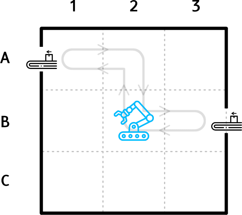
(a) A strategy satisfying the specification from Example 27 is highlighted.

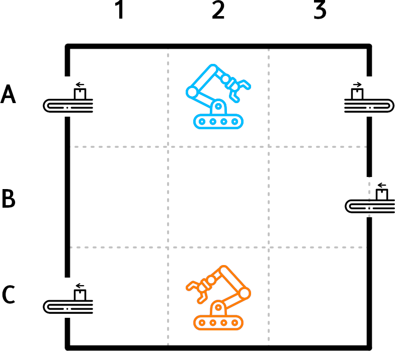
(b) Part of the extended factory discussed in Example 28.

Figure 6: Illustration of an automated factory with two mobile robots ${\color[rgb]{0,0.75,1}\mathcal{R}_{1}}$ and ${\color[rgb]{1,0.49609375,0}\mathcal{R}_{2}}$, discussed in Example 26-28. Cell $\Gamma_{i}$ is located in line $\Gamma\in\{A,B,C\}$ and row $i\in\{1,2,3\}$. Walls are indicated by solid lines, conveyor belts are depicted schematically.

The problem of synthesizing a logical controller for each component (i.e., a mission controller for each robot within Example 26) which ensures that logical (mission) specifications $\varphi_{i}$ are realized, can be modeled as a game. Here, the graph of this game models the interaction of the existing technical components (e.g., the robots) within their shared environment (e.g., their workspace). Logical (mission) specifications for different components are then naturally expressed via propositions that are defined over sets of states of this shared underlying game graph (as illustrated in Example 26), without changing its structure. This naturally leads to the two-objective (parity) games which we use as a starting point for synthesis.

While this reduces the need to create a game from a given LTL specification prior to synthesis, the requirements on both the synthesis procedure and the synthesized controllers are typically different from the requirements in “classical” (distributed) reactive synthesis.

The first major benefit of our method, compared to the existing approaches in [17, 27], is the computation of strategy templates which collect a (possibly infinite) number of strategies, instead of a single (coupled) strategy profile. This allows for easy adaptation and robustness of local controllers, as illustrated again via our factory example.

Example 27.

For simplicity, let us consider the scenario when the factory only has ${\color[rgb]{0,0.75,1}\mathcal{R}_{1}}$ (see Fig. 6(a)). In order to complete its task, the robot can use the strategy which keeps cycling along the path $A_{1}\rightarrow A_{2}\rightarrow B_{2}\rightarrow B_{3}\rightarrow B_{2}\rightarrow A_{2}\rightarrow A_{1}$. This strategy is fixed, and thereby does not allow easy modification when scenarios change. For example, suppose that the factory grows and another production machine is installed that takes the raw goods at $A_{3}$, which ${\color[rgb]{0,0.75,1}\mathcal{R}_{1}}$ too needs to collect and deposit as well. In standard methods, we would need to recompute a strategy for the new conjunctive objective $\varphi_{1}\wedge\varphi_{1}^{\prime}$ with $\varphi_{1}^{\prime}=\square\lozenge A_{3}$. In general, these computations are expensive and when more objectives are added, this gets impractical very quickly.

However, our templates mitigate this issue. As noticeable from the example, ${\color[rgb]{0,0.75,1}\mathcal{R}_{1}}$ does not really need to follow the path, and instead, only needs to always eventually go from $A_{1}$ to $A_{2}$ or $B_{1}$, from $A_{2}$ and $B_{1}$ to $A_{3}$ or $B_{2}$, from $A_{3}$ and $B_{2}$ to $B_{3}$, and so on. This is a sufficient liveness property that ${\color[rgb]{0,0.75,1}\mathcal{R}_{1}}$ needs to satisfy its initial objective $\varphi_{1}$. This property can be formalized as a strategy template (in particular via a live-group) and allows ${\color[rgb]{0,0.75,1}\mathcal{R}_{1}}$ to choose from different strategies fulfilling this template. Now a similar template can easily and independently be computed for the additional specification $\varphi_{1}^{\prime}$ when the new machine is installed. Then both templates can easily be composed by conjuncting all present liveness properties and ${\color[rgb]{0,0.75,1}\mathcal{R}_{1}}$ can choose a strategy that satisfies both objectives by complying with all these properties. E.g., at $B_{2}$, sometimes go to $A_{2}\rightarrow A_{1}$, sometimes to $A_{2}\rightarrow A_{3}$, and sometimes to $B_{3}$. Moreover, since templates do not fix a particular strategy and just act as a guidance system for the robot, they additionally provide fault-tolerance to the robot. Suppose due to some reason (presence of other robots), $A_{1}$ is momentarily blocked due to maintenance, then the robot can keep visiting $B_{3}$ and $A_{3}$, and when $A_{1}$ becomes available, it can continue visiting $A_{1}$.

While the above example illustrates the flexibility of strategy templates for a single component, their easy compositionality and adaptability enables an efficient negotiation framework, which we have formalized in the previous sections. We now illustrate this again with our running example.

Example 28.

We first observe that robot ${\color[rgb]{0,0.75,1}\mathcal{R}_{1}}$ has no strategy on its own to satisfy its respective objectives (if ${\color[rgb]{1,0.49609375,0}\mathcal{R}_{2}}$ always stays in $B_{3}$ blocking ${\color[rgb]{0,0.75,1}\mathcal{R}_{1}}$ from taking the raw material). Hence, the standard synthesis techniques will fail to give a controller for ${\color[rgb]{0,0.75,1}\mathcal{R}_{1}}$. However, since both robots are built by the factory designers, they can be made to cooperate instead of blocking the others. We therefore assume that ${\color[rgb]{0,0.75,1}\mathcal{R}_{1}}$ can “ask” ${\color[rgb]{1,0.49609375,0}\mathcal{R}_{2}}$ to always eventually leave $B_{3}$, so ${\color[rgb]{0,0.75,1}\mathcal{R}_{1}}$ can collect the raw goods. This leads us to the notion of adequately permissive assumptions (as in Definition 12) which can be computed using the algorithms in Section 5. Then both robots can compose their winning strategies with the assumption templates provided by the other agents, using the negotiation algorithm in Section 6, and play according to the obtained template. In our running example, this would lead to a compatible pair of csm’s where ${\color[rgb]{0,0.75,1}\mathcal{R}_{1}}$ goes to $A_{1}$ when ${\color[rgb]{1,0.49609375,0}\mathcal{R}_{2}}$ is at $B_{3}$, and goes to $B_{3}$ only when the access is granted by ${\color[rgb]{1,0.49609375,0}\mathcal{R}_{2}}$ (which ${\color[rgb]{1,0.49609375,0}\mathcal{R}_{2}}$ will grant, by following the final template), and will also let ${\color[rgb]{1,0.49609375,0}\mathcal{R}_{2}}$ go to $B_{3}$ always eventually when it arrives.

Summarizing the above factory example, the key idea of our framework lies in the use of strategy & assumption templates which allow for easy adaptability both (i) during synthesis and (ii) at runtime. During synthesis, this adaptability allows for mostly local and decentralized synthesis. Hence, in comparison to [17], components do not need to share their mission specifications or their final strategy choices which addresses specification- and strategy-related privacy concerns. In addition, by ensuring templates to be adequately permissive we still obtain a complete and surely terminating synthesis framework, which is in contrast to [27] which has no termination guarantees. During runtime, the adaptability of templates allows both for strategy adaptation and robustness, which is not present in neither [17] nor [27].

In the next sections we present more details on these distinguishing features of our framework in the context of logical control design for CPS. We further provide empirical evidence that our negotiation framework possess desirable computational properties by comparing our C++-based prototype tool CoSMo (Contracted Strategy Mask Negotiation) with state-of-the-art solvers.

7.2 Factory Benchmark

Motivated by the running example in Section 7.1, we consider a simplified factory set-up depicted in Fig. 7 (left) along with an automated benchmark generator to generate problem instances with different computational difficulty. The benchmark generator takes four parameters to change the characteristics of the game graph: the number of columns $x$, the number of rows $y$, the number of walls $w$, and the maximum number of one-way corridors $c$. Given these parameters, the workspace of the robots is constructed as follows: first, $w$ horizontal walls, i.e., walls between two adjacent rows, are generated randomly. We ensure that there is at least one passage from every row to its adjacent rows (if this is not possible with the given $w$, then $w$ is set to the maximum possible number for the given $x$ and $y$). Next, for each passage from one row to another, we randomly designate it to be a one-way corridor. For example, if a passage is an up-corridor, then the robots can only travel in the upward direction through this passage. We ensure that the maze has at most $c$ one-way corridors. An example of a benchmark maze with parameters $x=3$, $y=3$, $w=3$, and $c=2$ is shown in Fig. 7 (left). Given such a maze, we generate a game graph for two robots, denoted $R_{1}$ and $R_{2}$, that navigate the maze starting at the lower-left and lower-right corners of the maze, respectively. In this scenario the robots only interact explicitly via their shared workspace, i.e., possibly blocking each others way to the target.

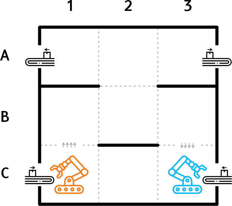
Figure 7: Left: Example of a benchmark maze with parameters $x=3$, $y=3$, $w=3$, and $c=2$. Solide lines denote walls, little up- and downward pointing arrows indicate one-way corridors. Right: Data points for benchmark mazes with Büchi objectives (blue circles) and parity objectives (green triangles) describing average execution time over all instances with the same grid size. The $y$-axis is given in log-scale.

7.2.1 Experimental Results

We have developed a C++-based prototype tool CoSMo that implements the negotiation algorithm (Algorithm 4) for solving two-objective parity games. All experiments were performed on a computer equipped with an Apple M1 Pro 8-core CPU and 16GB of RAM.

In a first set of experiments, we have have run CoSMo on a representative class of $2357$ benchmark instances generated as discussed before with two types of objectives. First, we consider the Büchi objective that robots $R_{1}$ and $R_{2}$ should visit the upper-right and upper-left corners, respectively, of the maze infinitely often, while ensuring that they never occupy the same location simultaneously and do not bump into a wall. Second, we consider the parity objectives from Example 26. We summarize our experimental results in Appendix B, Table 1 and plot all average run-times per grid-size (but with varying parameters for $c$ and $w$) in Fig. 7 (right). We see that CoSMo takes significantly more time for parity objectives compared to Büchi objectives. That is because computing templates for Büchi games takes linear time in the size of the games whereas the same takes biquadratic time for parity games (as shown in Theorem 16 and Theorem 18). Furthermore, the templates computed for Büchi objectives do not contain co-liveness templates, and hence, they do not not raise any conflict in most cases. However, tamplates for parity objectives contain all types of templates and hence, needs several rounds of negotiations to ensure conflict-freeness of the templates.

In a second set of experiments, we compared the performance of CoSMo, with the related tool agnes implementing the contract-based distributed synthesis method discussed from [27]. Unfortunately, agnes can only handle Büchi specifications and resulted in segmentation faults for many benchmark instances, in particular for non-trivial $c$ parameters. We have therefore always selected $c=0$ and only report computation times for all instances that have not resulted in segmentation faults.

The experimental results are summarized in Fig. 8-9 and LABEL:table:agnesVScosmo. As CoSMo implements a complete algorithm, it provably only concludes that a given benchmark instance is unrealizable, if it truly is unrealizable, i.e., for $1.67\%$ of the considered $120$ instances. agnes however, concludes unrealizability in $36,67\%$ of its instances (see Fig. 8 (left)), resulting an many false-negatives. Similarly, as CoSMo is ensured to always terminate, we see that all considered instances have terminated in the given time bound. While, agnes typically computes a solution faster for a given instance (see Fig. 9 (left)), it enters a non-terminating negotiation loop in $13,34\%$ of the instances (see Fig. 8 (right)). This happends for almost all considered gid sizes, as visible from Fig. 9 (right) where all non-terminating instances are included in the average after being mapped to $300s$, which was used as a time-out for the experiments.

Figure 8: Left: Percentage of instances on which the respective tool reports unrealizability after termination. Right: Percentage in which the respective tool does not terminate. Both numbers are mutually exclusive.

While our experiments show that agnes outperforms CoSMo in terms of computation times when it terminates on realizable instances (see Fig. 9 (left)), it is unable to synthesize strategies either due to conservatism or non-termination in almost $50\%$ of the considered instances (in addition to the ones which returned segmentation faults and which are therefore not included in the results). In addition to the fact that agnes can only handle the small class of Büchi specifications while CoSMo can handle parity objectives, we conclude that CoSMo clearly solves the given synthesis task much more satisfactory.

Figure 9: Average computation times over all instances with the same grid size for CoSMo (blue circles) and agnes (red squares) without timed-out instances (left) and with timed-out instances mapped to the time-out of $300s$ (right). The y-axis is given in log-scale.

7.3 Incremental Synthesis and Negotiation

While the previous section evaluates our method for a single, static synthesis task, we want to now emphasize the strength of our technique for the online adaptation of strategies. We therefore assume that Algorithm 4 has already terminated on the input $(G,\Phi_{0},\Phi_{1})$ and compatible csm’s $(\Psi_{0},\Pi_{0})$ and $(\Psi_{1},\Pi_{1})$ have been obtained. Then a new objective $\Phi_{i}^{\prime}$ arrives for component $i$.

As motivated in Section 7.1, we assume that this new specification again uses propositions that can be interpreted over the existing game graph $G$ (e.g., only consider new targets to be visited by the robots). We therefore treat the new task as an additional parity objective $\mathbb{P}_{i}^{\prime}$ over $G$ and compute an additional csm $(\Psi^{\prime}_{i},\Pi^{\prime}_{i}):=\textsc{ParityTemp}(G,\mathbb{P}^{\prime}_{i},i)$ for component $i$. It is easy to observe that if $(\Psi^{\prime}_{i},\Pi^{\prime}_{i})$ does not introduce new conflicts (i.e., $\Psi_{i}\wedge\Psi^{\prime}_{i}\wedge\Pi_{i-1}$ and $\tilde{\Pi_{i}}:=\Pi_{i}\wedge\Pi_{i}^{\prime}\wedge\Psi_{i-1}$ are still conflict-free), no further negotiation needs to be done and the csm of component $i$ can simply be updated to $(\Psi_{i}\wedge\Psi^{\prime}_{i},\Pi_{i}\wedge\Pi_{i}^{\prime})$. Otherwise, we simply re-negotiate by running more iterations of Algorithm 4. This is formalized in Algorithm 5 where we again slightly abuse notation as discussed in Remark 22.

Algorithm 5 $\textsc{Compose}(G,(\Phi_{0}^{j},\mathcal{W}^{j},\mathcal{C}^{j},\Pi^{j},\Psi^{j})_{j\leq\ell_{0}},(\Phi_{1}^{j},\mathcal{W}^{j},\mathcal{C}^{j},\Pi^{j},\Psi^{j})_{\ell_{0}<j<\ell},\Phi_{i}^{\ell})$

1:A game graph $G=(V,E)$; for each previous objective, a tuple containing the modified objective $\Phi_{i}^{j}$ with its winning region $\mathcal{W}^{j}$, co-Büchi region $\mathcal{C}^{j}$, assumption template $\Psi^{j}$, strategy template $\Pi^{j}$; and a new objective $\Phi_{i}^{\ell}$ such that $\Phi_{i}^{j}=\mathit{Parity}(\mathbb{P}_{i}^{j})$ with $\mathbb{P}_{i}^{j}:V\rightarrow[0;2d^{j}+1]$.

2:A tuple for each objective as in the input.

3:$(\mathcal{W}^{\ell},\mathcal{C}^{\ell},\Psi^{\ell},\Pi^{\ell})\leftarrow\textsc{ParityTemp}(G,\mathbb{P}_{i}^{\ell},i)$

4:while $\neg\textsc{CheckTemplate}\left(G,\bigwedge_{j\leq\ell}\left(\Pi^{j}\wedge\Psi^{j}\right)\right)$ do

5:     $\mathcal{W}\leftarrow\bigcap_{j\leq\ell}\mathcal{W}^{j}$; $\mathcal{C}\leftarrow\bigcup_{j\leq\ell}\mathcal{C}^{j}$

6:     $\Phi_{0}^{j}\leftarrow\square\mathcal{W}\wedge Parity(\mathbb{P}^{j}[\mathcal{C}\rightarrow 2d^{j}+1])$ for $j\leq\ell_{0}$

7:     $\Phi_{1}^{j}\leftarrow\square\mathcal{W}\wedge Parity(\mathbb{P}^{j}[\mathcal{C}\rightarrow 2d^{j}+1])$ for $\ell_{0}<j\leq\ell$

8:     $\mathcal{W}^{j},\mathcal{C}^{j},\Pi^{j},\Psi^{j}\leftarrow\textsc{ParityTemp}(G,\Phi_{0}^{j},0)$ for each $j\leq\ell_{0}$

9:     $\mathcal{W}^{j},\mathcal{C}^{j},\Pi^{j},\Psi^{j}\leftarrow\textsc{ParityTemp}(G,\Phi_{1}^{j},1)$ for each $\ell_{0}<j\leq\ell$

10:return $(\Phi_{0}^{j},\mathcal{W}^{j},\mathcal{C}^{j},\Pi^{j},\Psi^{j})_{j\leq\ell_{0}},(\Phi_{1}^{j},\mathcal{W}^{j},\mathcal{C}^{j},\Pi^{j},\Psi^{j})_{\ell_{0}<j\leq\ell}$

The intuition behind Algorithm 5 is as follows. If no partial solution to the synthesis problem exists so far we have $\ell_{i}=0$ for each $i\in\{0,1\}$, otherwise the game $(G,\bigwedge_{j\leq\ell_{0}}\Phi_{0}^{j},\bigwedge_{\ell_{0}<j<\ell}\Phi_{1}^{j})$ was already solved and the respective winning region, co-Büchi region, and templates are known. In both cases, the algorithm starts with computing a csm for the game $(G,\Phi_{i}^{\ell})$ (line 1) and checks for conflicts (line 2). If the csm’s have conflicts, the algorithm modifies the objectives as in Algorithm 4 to ensure that the losing regions are never visited and the co-Büchi regions are eventually not visited anymore (lines 4-5), and then re-computes the templates (line 6-7) to check for conflicts again.

The correctness of Algorithm 5 is formalized in the following corollary which directly follows from Theorem 23 due to the fact that Algorithm 5 only outputs conflict-free csm’s.

Corollary 29.

Given a game $\mathcal{G}=(G,\bigwedge_{j\leq\ell_{0}}\Phi_{0}^{j},\bigwedge_{\ell_{0}<i\leq\ell}\Phi_{1}^{j})$, Compose always terminates in $\mathcal{O}(\ell n^{6})$ time, where $n=\left\lvert V\right\rvert$. Moreover, if Compose returns the tuples $(\Phi_{0}^{j},\mathcal{W}^{j},\mathcal{C}^{j},\Pi^{j},\Psi^{j})_{j\leq\ell_{0}},(\Phi_{1}^{j},\mathcal{W}^{j},\mathcal{C}^{j},\Pi^{j},\Psi^{j})_{\ell_{0}<j\leq\ell}$ by incrementally adding objectives $\Phi_{i}^{j}$ one by one, then a strategy profile $(\pi_{0},\pi_{1})$ is winning for $\mathcal{G}$ if for each $i\in\{0,1\}$, $\pi_{i}$ follows every strategy template $\Pi^{j}$ computed for $\text{Player}\leavevmode\nobreak\ i$ objective $\Phi_{i}^{j}$ along with every assumption template $\Psi^{j}$ computed for $\text{Player}\leavevmode\nobreak\ 1-i$ objective $\Phi_{1-i}^{j}$.

7.3.1 Experimental Evaluation

As our competing tool agnes already showed subpar performance in Section 7.2.1 and does not feature strategy templates for easy adaptation, we refrain from comparing the incremental version of our tool CoSMo (implementing incremental negotiation and synthesis as in Algorithm 5) to the re-application of agnes whenever a new objective arises. Instead, we note that, algorithmically, we are solving a cooperative generalized parity game, i.e., a cooperative parity game with a conjunction of a finite number of parity objectives, in an incremental fashion. We therefore compare the performance of CoSMo on such synthesis problems to the best known solver for generalized parity games, i.e, genZiel from [14] (implemented by [10]).

To allow for a better interpretation our experimental results, we note the following observations. First, similar to our approach, genZiel is based on Zielonka’s algorithm. However, it solves one centralized cooperative game for the conjunction of all players objectives, while our approach solves zero-sum games locally only for the local objectives, allowing objectives and strategies to be kept mostly private. Second, genZiel only outputs a single cooperative strategy profile after termination. While this prevents the usage of strategies in a fault-tolerant fashion (as exemplified in Section 7.4), it also implies that genZiel needs to recompute a new strategy profile whenever a new specification arises, without re-using any information from previous computations. Third, while we have already compared the one-sided version of our tool, called PeSTel with genZiel for a single zero-sum generalized parity game in [6], where our method was (in comparison to genZiel) not complete, we note that in the setting presented in this paper, both CoSMo and genZiel are sound and complete, i.e., return winning strategies iff there exists a cooperative solution to the given two-objective game.

Finally, due to the nature of Zielonka’s algorithm and the centralized synthesis within genZiel, the latter tool terminates very quickly if the cooperative winning region is empty. While this could be added as a pre-processing step, this is not yet true for CoSMo, as its computations are decentralized. As more conjuncted specifications result in a highly likelyhood of the winning region to be empty, it is not surprising that our comparative evaluation becomes somewhat meaningless if too many objectives are added. In order to separate the effect of (i) the increased number of re-computation and (ii) the shrinking of the winning region, induced by an increased number of incrementally added objectives, we consider a slightly more elaborate case-study compared to [6]. Instead of blindly adding more and more (randomly generated) parity objectives, we allow objectives to disappear again after some time (which is also very natural in the robotic context discussed in Section 7.1).

Benchmark generation. We have generated $2244$ benchmarks from the games used for the Reactive Synthesis Competition (SYNTCOMP) [20] by adding randomly generated parity objectives to given parity games. The random generator takes two parameters: game graph $G$ and maximum priority $m$; and then it generates a random parity objectives with maximum priority $m$ as follows: 50% of the vertices in $G$ are selected randomly, and those vertices are assigned priorities ranging from $0$ to $m$ (including $0$ and $m$) such that $1/m$-th (of those 50%) vertices are assigned priority $0$ and $1/m$-th are assigned priority $1$ and so on. The rest 50% are assigned random priorities ranging from $0$ to $m$. Hence, for every priority, there are at least $1/(2m)$-th vertices (i.e., $1/m$-th of 50% vertices) with that priority.

Figure 10: Experimental results over $2244$ games with multiple parity objectives comparing the performance of our tool CoSMo (indicated by blue circles) against the state-of-the-art tool for solving games with multiple parity objectives genZiel [14] (indicated by red squares). Data points give the average execution time (in ms) over all instances with the same number of parity objectives when the objectives are added incrementally one-by-one.

Figure 11: Experimental results comparing the performance of our tool CoSMo (indicated by blue circles) against the state-of-the-art tool for solving games with multiple parity objectives genZiel [14] (indicated by red squares) for games with either $5$ (left) or $6$ (right) long-term objectives with one temporary objective added (and removed again) in each iteration. Data points give the average execution time (in ms) over all instances with the same number of iterations.

Comparative evaluation. All experiments were performed on a computer equipped with Apple M1 Pro 8-core CPU and 16GB RAM. We performed two kinds of experiments.

First, we solved the benchmarks by adding the objectives incrementally one-by-one, i.e., we solved the game with $\ell$ objectives, then we added one more objective for $\text{Player}\leavevmode\nobreak\ 1$ and solved it again, and so on. The results are summarized in Fig. 10. We see that for a low number of objectives, the negotiation of contracts in a distributed fashion by CoSMo adds computational overhead compared to genZiel, which reduces when more objectives are added. However, as more objectives are added the chance of the winning region to become empty increases. Further, typically more and more conflicts arise if more specifications are combined so that CoSMo needs to recompute more often. This results in both lines to eventually become closer again. Nevertheless, we want to emphasize that this experiment also shows that even though CoSMo performs strategy computations in a decentralized manner and computes strategy templates instead of a single strategy profile, it shows similar and often superior performance compared to the highly optimized and centralized genZiel algorithm.

Second, in order to rule out the competing effect of an empty winning region when too many objectives are added (given genZiel a clear advantage, as discussed above), we considered benchmarks which have a fixed number of long-term objectives, and then we iteratively add just one temporary objective. The results are summarized in Fig. 11 when the number of long-term objectives are $5$ (left) and $6$ (right), and we have added one temporary objective in each iteration, after removing the temporal objective (along with all its templates) from the previous iteration. We see that in this scenario the advantage of CoSMo to avoid re-computations whenever no conflicts arrise is present more frequently, showing that the gap between the performance of both tools increases with the number of new specifications.

7.4 Fault-Tolerant Strategy Adaptation

While the previous sections outline the computational tractability of our decentralized, negotiation-based synthesis framework, this section shows the additional benefit obtained by using strategy templates within control implementations during runtime.

As already discussed in Example 27, controlled technical components might face restrictions in their moves during runtime (e.g., due to blocked pathways or miss-function of motors on certain wheels within the robot example). These restrictions are generally called actuator faults in the control community.

Intuitively, the permissiveness of our strategy templates allows a controller to be more robust against actuator faults, by offering more choices to handle unavailable strategy choices.

The simplest instance of this problem is given if a certain set of actuators is known to possibly become persistently unavailable, i.e. certain edges from player $0$ vertices will potentially disappear permanently. Then such faults can simply be modelled as additional safety specifications over the systems. Suppose $\mathcal{F}$ is a subset of $\text{Player}\leavevmode\nobreak\ 0$ edges (analogous for $\text{Player}\leavevmode\nobreak\ 1$), such that edges from $\mathcal{F}$ may disappear during runtime. Then using the CheckTemplate procedure, $\text{Player}\leavevmode\nobreak\ 0$ can check if their existing templates from a csm conflicts with $\Lambda_{\textsc{unsafe}}(\mathcal{F})$. If there are no conflicts, $\text{Player}\leavevmode\nobreak\ 0$ can simply switch to another strategy using the ExtractStrategy procedure from Section 6.3 under the added safety template. If there are conflicts, both agents need to renegotiate (using incremental negotiation and synthesis as in Algorithm 5).

In the above mentioned approach, the systems treats the potentially faulty edges as unsafe edges and hence never takes such edges. In real-life, however, it might not be known which actuators will fail – most of the time actually all actuators might fail – making a worst-case analysis return no controller at all. It is therefore often desirable to take favorable actions as long as they are actually available. Formally, this scenario can be defined via a time-dependent graph whose edges change over time, i.e., $E^{t}$ with $E^{0}=E$ are the edges available at time $t\in\mathbb{N}$ and $\mathcal{F}:=\{e\in E\mid e\not\in E^{t},\text{ for some }t\}$. Given the original game $\mathcal{G}=(G,\Phi_{0},\Phi_{1})$ with a compatible csm contract $\mathtt{C}$ we can easily modify $\textsc{ExtractStrategy}(\mathcal{G},\Lambda)$ to obtain a time-dependent strategy $\pi_{g}$ which reacts to the unavailability of edges, i.e., at time $t$, $\pi_{g}$ takes an edge $e\in E^{t}\backslash(S\cup D)$ for all vertices without any live-group, and for the ones with live-groups, it alternates between the edges satisfying the live-groups whenever they are available, and an edge $e\in E^{t}\backslash(S\cup D)$ when no live-group edge is available. The reader should notice that $\pi_{g}$ can be obtained in linear time.

The online strategy $\pi_{g}$ can be implemented even without knowing when edges are available, i.e., without knowing the time dependent edge sequence $\left\{E^{t}\right\}_{t\in\mathbb{N}}$ up front. In this case $\pi_{g}$ is obviously winning in $\mathcal{G}=(G,\mathit{Parity}(\mathbb{P}))$ if $\Psi$ is conflict-free for $\mathcal{G}|_{E\setminus F}$. If this is not the case, the optimal recomputation is non-trivial and is out of scope of this paper. We can however collect the vertices which do not satisfy the above property and alert the system engineer that these vulnerable actuators require additional maintenance or protective hardware. We have shown with experiments over a large benchmark set in [6], Sec. 6, that typically less then $5\%$ of the vertices are vulnerable and, hence, protecting them is typically reasonable in practice.

8 Summary and Future Work

This paper provides a new framework for distributed, contract-based strategy synthesis in two-objective parity games. The key idea of this framework, which distinguishes it from existing works, lies in the use of strategy & assumption templates which allow for easy adaptability both (i) during synthesis and (ii) at runtime. This leads to a distributed algorithm which computes strategies locally, but still ensures completeness and guaranteed termination (given enough computational resources). In particular, we have shown the effective applicability of our method to synthesis problems in CPS design.

Arguably, the main draw-back of our method is its need to consider a common shared game graph, and hence imposes the requirement of full information, which is not needed in other competing works. We leave the problem of utilizing the adaptability and locality of templates for distributed synthesis under partial observation for future work. While this setting clearly does not allow for completness, we believe that in most scenarios where the resulting need for cooperation is restricted to observable states (e.g., when robots are in each others vicinity and know their respective location) our method will provide interesting new solutions, in particular in the context of CPS design. Another interesting direction is to explore the integration of qualitative objectives to pic strategies from strategy templates after negotiation has terminated. Similarly, timing aspects both within the model or the specifications are interesting directions for future work.

In summary, we believe that the use of templates provides a novel attack angle for the problem of distributed synthesis which seems promising for many problems in CPS design that require robustness and adaptation beyond what can be provided by current reactive synthesis engines.

Appendix A Additional Proofs for Section 5

A.1 Proof of Theorem 16

See 16

Proof.

We first show that the algorithm terminates. We show that the procedure Live terminates. Since in 5, the game graph is restricted to cooperative Büchi winning region $Z^{*}$, we need to show that in the procedure, $U=V=Z^{*}$ eventually. Let $U_{l}$ be the value of $U$ after the $l$-th iteration of $\textsc{Live}(G,I,i)$, with $U^{0}=I$. Since vertices are only added to $U$ (and never removed) and there are only finitely many vertices, $U_{0}\subseteq U_{1}\subseteq\ldots\subseteq U_{m-1}=U_{m}$ for some $m\in\mathbb{N}$.

Since the other direction is trivial, we show that $Z^{*}\subseteq U_{m}$. Suppose this is not the case, i.e. $v\in Z^{*}\backslash U_{m}$. Since $v\in Z^{*}$, both players cooperately can visit $I$ from $v$. Then there is a finite path $\rho=v=v_{0}v_{1}\cdots v_{k}$ for $v_{k}\in I$. But since $I=U_{0}\subseteq U_{m}$, but $v\not\in U_{m}$, $\rho$ enters $U_{m}$ eventually. Let $l$ be the highest index such that $v_{l}\not\in U_{m}$ but $v_{l+1}\in U_{m}$.

Then if $v_{l}\in V_{i}$, it would be added to $U$ in 15 of $(m+1)$-th iteration, i.e. $U_{m}\not=U_{m+1}$. Else if $v_{l}\in V_{1-i}$, it would be added to $U$ in 18 of $(m+1)$-th iteration since $v_{l+1}\in U_{m}$, i.e. $U_{m}\not=U_{m+1}$. In either case, we get a contradiction. Hence, $v\in U_{m}$, implying $Z^{*}=U_{m}$. Hence the procedure Live, and hence Algorithm 1, terminates.

We now show that the csm obtained is adequately permissive for $\text{Player}\leavevmode\nobreak\ i$.

$\blacktriangleright$ (ii)Implementability: We first show that $\mathopen{\hbox{\set@color${\langle}$}\kern-1.94444pt\leavevmode\hbox{\set@color${\langle}$}}1-i\mathclose{\hbox{\set@color${\rangle}$}\kern-1.94444pt\leavevmode\hbox{\set@color${\rangle}$}}\Psi=V$, but since the forward containment is trivial, we show $\mathopen{\hbox{\set@color${\langle}$}\kern-1.94444pt\leavevmode\hbox{\set@color${\langle}$}}1-i\mathclose{\hbox{\set@color${\rangle}$}\kern-1.94444pt\leavevmode\hbox{\set@color${\rangle}$}}\Psi\supseteq V$. We note that in 16, $C\subseteq V_{1-i}$: since if $v\in V_{i}\cap C$, then there is an edge from $v$ to $U$, and hence $v\in U$ already by 13 and 15. Then since the source of live groups (which are only added in 17) is a subset of $\text{Player}\leavevmode\nobreak\ 1-i$’s vertices, then if $\text{Player}\leavevmode\nobreak\ 1-i$ plays one of these live group edges infinitely often, when the sources are visited infinitely often, $\text{Player}\leavevmode\nobreak\ i$ can not falsify it, and hence $\mathopen{\hbox{\set@color${\langle}$}\kern-1.94444pt\leavevmode\hbox{\set@color${\langle}$}}1-i\mathclose{\hbox{\set@color${\rangle}$}\kern-1.94444pt\leavevmode\hbox{\set@color${\rangle}$}}\Psi\supseteq V$. Analogously, $\mathopen{\hbox{\set@color${\langle}$}\kern-1.94444pt\leavevmode\hbox{\set@color${\langle}$}}i\mathclose{\hbox{\set@color${\rangle}$}\kern-1.94444pt\leavevmode\hbox{\set@color${\rangle}$}}\Pi\supseteq V$, since in Line 14, live group edges are added only from $\text{Player}\leavevmode\nobreak\ i$’s vertices, by definition of $\textsc{Attr}_{i}$. $\blacktriangleright$ (i)Sufficiency: Again, let $U_{l}$ and $m$ be as defined earlier. Define $X_{l}\coloneqq U_{l}\backslash U_{l-1}$ for $1\leq l\leq m$, and $X_{0}=U_{0}=I$. Then every vertex $v\in Z^{*}$ is in $X_{l}$ for some $l\in[0;m]$. Consider the strategy $\pi_{i}$ for $\text{Player}\leavevmode\nobreak\ i$: at a vertex $v\in V_{i}\cap X_{l}$, she plays the $\textsf{attr}^{i}$ strategy to reach $U_{l-1}$, and for other vertices, she plays arbitrarily. It is easy to observe that $\pi_{i}$ follows $\Phi$. Then we show that for any $\text{Player}\leavevmode\nobreak\ 1-i$ strategy $\pi_{j}$ following $\Psi$, the resulting $\pi_{i}\pi_{j}$-play $\rho$ from any $v_{0}\in Z^{*}$ belongs to $\mathcal{L}(\Phi)$. Let $v_{0}\in Z^{*}=\mathopen{\hbox{\set@color${\langle}$}\kern-1.94444pt\leavevmode\hbox{\set@color${\langle}$}}0,1\mathclose{\hbox{\set@color${\rangle}$}\kern-1.94444pt\leavevmode\hbox{\set@color${\rangle}$}}\square\lozenge I$ (from 3). Let $\pi_{j}$ be an arbitrary strategy that follows $\Psi$, and $\rho=v_{0}v_{1}\ldots$ be an arbitrary $\pi_{i}\pi_{j}$-play. Then $\rho\in\mathcal{L}(\Psi)$. It remains to show that $\rho\in\mathcal{L}(\Phi)$. Suppose $\rho\not\in\mathcal{L}(\Phi)$, i.e. $inf(\rho)\cap I=\emptyset$. Note that $\rho$ never leaves $Z^{*}$ due to safety assumption template. Then consider the set $R$ of vertices which occur infinitely often in $\rho$. Let $0\leq k\leq m$ be the least index such that $R\cap X_{k}\not=\emptyset$. From the assumption, $k>0$. Let $v\in R\cap X_{k}$. If $v\in V_{i}$, by the definition of $\pi_{i}$, every time $\rho$ reaches $v$, it must reach $U_{k-1}$, contradicting the minimality of $k$. Else if $v\in V_{1-i}$, then by the definition of $H_{\ell}^{a}$, infinitely often reaching $v$ implies infinitely often reaching $\textsf{attr}_{i}(U_{k-1})$. But again the play visits $U_{k-1}$ by arguments above, giving the contradiction. In any case, we get a contradiction, implying that the assumption is wrong. Hence, $\rho\in\mathcal{L}(\Phi)$, and $v_{0}\in\mathopen{\hbox{\set@color${\langle}$}\kern-1.94444pt\leavevmode\hbox{\set@color${\langle}$}}i\mathclose{\hbox{\set@color${\rangle}$}\kern-1.94444pt\leavevmode\hbox{\set@color${\rangle}$}}(\Psi,\Pi)$. $\blacktriangleright$ (iii)Permissiveness: Now for the permissiveness of the csm, let $\rho\in\mathcal{L}{(\Phi)}$. Suppose that $\rho\not\in\mathcal{L}{(\Psi)}$. Case 1: If $\rho\not\in\mathcal{L}{(\Lambda_{\textsc{unsafe}}(S^{a}))}$, then some edge $(v,v^{\prime})\in S^{a}$ is taken in $\rho$. Then after reaching $v^{\prime}$, $\rho$ still satisfies the Büchi condition. Hence, $v^{\prime}\in Z^{*}=\mathopen{\hbox{\set@color${\langle}$}\kern-1.94444pt\leavevmode\hbox{\set@color${\langle}$}}0,1\mathclose{\hbox{\set@color${\rangle}$}\kern-1.94444pt\leavevmode\hbox{\set@color${\rangle}$}}\square\lozenge I$, but then $(v,v^{\prime})\not\in S^{a}$, which is a contradiction. Case 2: If $\rho\not\in\mathcal{L}(\Lambda_{\textsc{live}}(H_{\ell}^{a}))$, then $\exists H_{i}\in H_{\ell}^{a},$ such that $\rho$ visits $src(H_{i})=C_{l}$ (for the value of C after $l$-th iteration) infinitely often, but no edge in $H_{i}$ is taken infinitely often. Then since the edges in $H_{i}$ lead to $\textsf{attr}^{U_{l-1}}_{i}()$, the play must stay in either $C_{l}$ or goes to $U^{k}\setminus U^{l}$ for some $k>l+1$. In the first case, since $I\cap Z^{*}\subseteq U^{0}$, $\rho\not\in\Phi$, which would be a contradiction. On the other hand, in the second case, after going to $U^{k}\setminus U^{l}$, $\rho$ has an edge going from some $v\in Z^{*}\backslash U^{k-1}$ to some $v^{\prime}\in U^{l}$ (else $I\cap Z^{*}\subseteq U^{0}\subseteq U^{l}$ can not be reached). But then $v$ would be added to $U^{k+1}$, which contradicts to the fact that $k>l+1$. In either case, we get a contradiction, so $\rho\in\mathcal{L}(\Psi)$. $\blacktriangleright$ Complexity analysis.The computation of cooperative winning region can be done in time linear in number of edges, i.e. $\mathcal{O}(m)$. The procedure Livetakes $\mathcal{O}(m)$ time. Hence, resulting in time linear in number of edges in the game graph.

∎

A.2 Proof of Theorem 17

See 17

Proof.

We first show that the algorithm terminates. We show that the procedure CoLive terminates when all the vertices of the game graph are cooperatively winning for the co-Büchi objective $\Phi_{i}=\lozenge\square I$, since we restrict the graph to the cooperative winning region in 5. We claim that $U=V=Z^{*}$, eventually.

Let $U_{l}$ be the value of the variable $U$ after $l$-th iteration of the while loop, with $U_{0}=\textsc{Safety}_{0,1}(G,I)$. Since vertices are only added in $U$, $U_{0}\subseteq U_{1}\subseteq\ldots\subseteq U_{k}=U_{k+1}$ for some $k\in\mathbb{N}$. Suppose $V\not\subseteq U_{k}$, then there exists $v\in V\backslash U_{k}$. Since $v\in Z^{*}$, there is a $\rho=vv_{1}v_{2}\ldots$ from $v$ to $U_{0}$ and stays there forever. Then consider the largest index $m$ such that $v_{m}\not\in U_{k}$, but $v_{m+1}\in U_{k}$. Note that this index exists because $U_{0}\subseteq U_{k}$. But then $v_{m}\in\textsf{pre}_{G}(U_{k})$, and hence $U_{k}\not=U_{k+1}$, which is a contradiction. Hence, our assumption that $v\not\in U_{k}$ is incorrect, implying that $U=V$ eventually.

Now we show that $\Psi$ is an adequately permissive assumption. Again, let $U_{l}$ and $m$ be as defined earlier. Define $X_{l}\coloneqq U_{l}\backslash U_{l-1}$ for $1\leq l\leq m$, and $X_{0}=U_{0}=I$. Then every vertex $v\in Z^{*}$ is in $X_{l}$ for some $l\in[0;m]$.

We again prove (i)-(iii) of Definition 12 separately and finally comment on the complexity of coBüchiTemp.

$\blacktriangleright$ (ii)Implementability: We again observe that the sources of the co-live edges in $D^{a}$ are $\text{Player}\leavevmode\nobreak\ 1-i$’s vertices and hence can be easily implemented by $\text{Player}\leavevmode\nobreak\ 1-i$, by taking those edges only finitely often. Similarly, the sources of the co-live edges in $D^{s}$ are $\text{Player}\leavevmode\nobreak\ i$’s vertices, giving the implementability of $\Pi$ by $\text{Player}\leavevmode\nobreak\ i$. $\blacktriangleright$ (i)Sufficiency: Consider the following strategy $\pi_{i}$ for $\text{Player}\leavevmode\nobreak\ i$: at a vertex $v\in X_{0}\cap V_{i}$, she takes edge $(v,v^{\prime})\in E$ such that $v^{\prime}\in X_{0}$, at a vertex $v\in X_{l}\cap V_{i}$, for $l\in[1;m]$, she plays the edges not in $S^{s}$ to reach $U_{l-1}$ (such edges exist by definition of $U_{l}$’s), and for all other vertices, she plays arbitrarily. Let $v_{0}\in Z^{*}=\mathopen{\hbox{\set@color${\langle}$}\kern-1.94444pt\leavevmode\hbox{\set@color${\langle}$}}0,1\mathclose{\hbox{\set@color${\rangle}$}\kern-1.94444pt\leavevmode\hbox{\set@color${\rangle}$}}\lozenge\square I$ (from 3). Let $\pi_{j}$ be an arbitrary strategy of $\text{Player}\leavevmode\nobreak\ 1-i$ following $\Psi$, and $\rho=v_{0}v_{1}\ldots$ be an arbitrary $\pi_{i}\pi_{j}$-play. Then $\rho\in\mathcal{L}(\Psi)$. It remains to show that $\rho\in\mathcal{L}(\Phi)$. Since $\rho\in\mathcal{L}(\Lambda_{\textsc{unsafe}}(S))$ and by definition of $\pi_{i}$, $v_{i}\in Z^{*}$ for all $i$. Now suppose $\rho\not\in\mathcal{L}(\Phi)$, i.e. $\inf(\rho)\cap(Z^{*}\setminus I)\not=\emptyset$. Let $u\in Z^{*}\setminus I$. Then to reach $u$ infinitely often some edge from $D^{a}$ must be taken infinitely often in $\rho$, since $\pi_{i}$ makes the play go towards $I$. But this contradicts the fact that $\rho\in\mathcal{L}(\Psi)$. Hence, $\rho\in\mathcal{L}(\Phi)$. $\blacktriangleright$ (iii)Permissiveness: Let $\rho=v_{0}v_{1}\ldots$ such that $v_{0}\in Z^{*}$ and $\rho\in\mathcal{L}(\Phi)$. Suppose that $\rho\not\in\mathcal{L}(\Psi)$. Case 1: If $\rho\not\in\Lambda_{\textsc{unsafe}}(S^{a})$. Then the same argument as in the Büchi case gives a contradiction. Case 2: If $\rho\not\in\Lambda_{\textsc{colive}}(D^{a})$, that is $\exists(u,v)\in D^{a},$ such that $\rho$ takes $(u,v)$ infinitely often. By the definition of $D^{a}$, $v\in Z^{*}\setminus U_{0}$, implying $v\not\in I$, since if $v\in I$ then it would have been in $U_{0}$. Hence, $\rho\not\in\mathcal{L}(\Phi)$, giving a contradiction. So $\rho\in\mathcal{L}(\Psi)$. $\blacktriangleright$ Complexity analysis.Very similar to that for Büchi objectives and therefore omitted.

∎

A.3 Proof of Theorem 18

See 18

Proof.

The termination of the algorithm follows from the termination of the ComputeSets procedure. Note that if the graph is either empty or if every vertex has priority 0, then the procedure terminates trivially. Now, in every iteration of the procedure, either at least a vertex is removed (if $d$ is odd, then $W_{\neg D}$ has fewer vertices) or the number of priority is reduced (if $d$ is even, then $G\mid_{W_{\neg D}}$ has fewer priorities). Then, after finitely many iterations, ComputeSets terminates.

We prove sufficiency, implementability and permissiveness below and then analyze the complexity of Algorithm 3.

$\blacktriangleright$ (ii)Implementability: We note that the assumption template $\Psi$ is implementable by $\text{Player}\leavevmode\nobreak\ 1-i$ due to the implementability of safety, liveness and co-liveness assumptions: if for a conditional live group, the corresponding vertex set is reached infinitely often, and also the sources of live groups are visited infinitely often, $\text{Player}\leavevmode\nobreak\ 1-i$ can choose the live group edges, since they are controlled by $\text{Player}\leavevmode\nobreak\ 1-i$. Moreover, there won’t be any conflict due to the live groups as there can be no unsafe or co-live edge that is included in a conditional live group by construction. Analogously, $\Pi$ is implementable by $\text{Player}\leavevmode\nobreak\ i$. $\blacktriangleright$ (i)Sufficiency: We give a strategy for $\text{Player}\leavevmode\nobreak\ 0$ depending on the parity of the highest priority $d$ occurring in the game and show that it is winning under assumption $\Psi$ for all vertices in the cooperative winning region $Z^{*}=\textsc{Parity}(G,\mathbb{P})$. The strategy uses finite memory and the winning strategies for $\text{Player}\leavevmode\nobreak\ 1$ in subgames with Büchi (Theorem 16) and co-Büchi (Theorem 17) objectives. By $\mathit{B\ddot{u}chi}(G,U)$, we denote the game $(G,\square\lozenge U)$, and by $\mathit{co\text{-}B\ddot{u}chi}(G,U)$, we denote the game $(G,\lozenge\square U)$. We also use the definitions of $d$, $W_{d}$ and $W_{\neg d}$, as in the Algorithm 3. Consider the following strategy $\pi_{0}$ of $\text{Player}\leavevmode\nobreak\ 0$: $\triangleright$ $d$is odd: If the play is in $V\setminus W_{\neg d}$, then $\text{Player}\leavevmode\nobreak\ 0$ plays the $\mathit{co\text{-}B\ddot{u}chi}(G,W_{\neg d})$ winning strategy to eventually end up in $W_{\neg d}$. If the play is in $W_{\neg d}\cap Z^{*}$, $\text{Player}\leavevmode\nobreak\ 0$ plays the recursive winning strategy for $(G|_{W_{\neg d}},\mathit{Parity}(\mathbb{P}))$. Otherwise, she plays arbitrarily. $\triangleright$ $d$is even: If the play is in $W_{d}$, $\text{Player}\leavevmode\nobreak\ 0$ switches its strategy among $\mathit{B\ddot{u}chi}(G,W_{d})$, $\mathit{B\ddot{u}chi}(G,W_{d}\cup W_{d-2})$, $\ldots$, $\mathit{B\ddot{u}chi}(G,W_{d}\cup W_{d-2}\cup\cdots W_{2})$ winning strategies, i.e., for each vertex, she first uses the first strategy in the above sequence, then when that vertex is repeated, she uses the second strategy for the next move, and keeps switching to the next strategies for every move from the same vertex. If the play is in $V\setminus W_{d}\cap Z^{*}$, then she plays the recursive winning strategy for $(G|_{W_{\neg d}},\mathit{Parity}(\mathbb{P}))$, where $\mathbb{P}$ is modified again as in 21. Otherwise, she plays arbitrarily. We prove by induction, on the highest occurring priority $d$, that the above constructed strategy $\pi_{0}$ for $\text{Player}\leavevmode\nobreak\ 0$ ensures satisfying the parity objective on the original game graph if the assumption $\Psi$ is satisfied. For the base case, when $d=0$, the constructed strategy is trivially winning, because the only existing color is even. Now let the strategy be winning for $d-1\geq 0$. Let $v_{0}\in Z^{*}=\textsc{Parity}(G,\mathbb{P})$. Let $\pi_{1}$ be an arbitrary strategy of $\text{Player}\leavevmode\nobreak\ 1$ following $\Psi$, and $\rho=v_{0}v_{1}\ldots$ be an arbitrary $\pi_{0}\pi_{1}$-play. Then $\rho\in\mathcal{L}(\Psi)$. We need to show that $\rho$ is winning, i.e., $\rho\in\mathcal{L}(\Phi)$. Note that by the safety assumption and by the construction of $\pi_{0}$, $\rho$ stays in the vertex set $Z^{*}$. Case 1: If $d$ is odd, then since at vertices in $V\setminus W_{\neg d}$, $\text{Player}\leavevmode\nobreak\ 0$ plays to eventually stay in $W_{\neg d}$, the play can not stay in $W_{\neg d}$ without violating $\Lambda_{\textsc{colive}}(D)$. And if $\rho$ eventually stays in $W_{\neg d}$, then by the induction hypothesis, it is winning, since $W_{\neg d}\cap P^{d}=\emptyset$. Case 2: If $d$ is even, then if the play stays in $W_{d}$ eventually, and if the play visits vertices of an odd priority $i$ infinitely often, then $\pi_{1}$ satisfies $\textsc{Live}(G,P^{i+1}\cup P^{i+2}\cup\cdots\cup P^{d},i)$ by the conditional live group assumption. Note that $\text{Player}\leavevmode\nobreak\ 0$ plays the $\mathit{B\ddot{u}chi}(G,P^{i+1}\cup P^{i+2}\cup\cdots\cup P^{d})$ winning strategy for infinitely many moves from every vertex occurring in $\rho$. Since $\pi_{1}$ satisfies $\textsc{Live}(G,P^{i+1}\cup P^{i+2}\cup\cdots\cup P^{d},i)$, after these moves as well, the play visits $(P^{i+1}\cup P^{i+2}\cup\cdots\cup P^{d})$. Hence the play will visit vertices of an even color $>i$ infinitely often, implying that $\rho$ is winning. Else if $\rho$ stays in $V\setminus W_{d}$ eventually, then it is winning by induction hypothesis. This gives the sufficiency of the csm computed by the algorithm. $\blacktriangleright$ (iii)Permissiveness: Now for the permissiveness of the csm, let $\rho\in\mathcal{L}(\Phi)$. We prove the claim by contradiction and suppose that $\rho\not\in\mathcal{L}(\Psi)$. Case 1: If $\rho\not\in\Lambda_{\textsc{unsafe}}(S)$. Then some edge $(v,v^{\prime})\in S$ is taken in $\rho$. Then after reaching $v^{\prime}$, $\rho$ still satisfies the parity objective. Hence, $v^{\prime}\in Z^{*}$, but then $(v,v^{\prime})\not\in S$, which is a contradiction. Case 2: If $\rho\not\in\Lambda_{\textsc{cond}}(\mathcal{H})$. Then for some even $j$ and odd $i<j$, $\rho$ visits $W_{j}\cap P^{i}$ infinitely often but does not satisfy the live transition group assumption $\textsc{Live}(G^{\prime},P^{i+1}\cup P^{i+2}\cdots\cup P^{j}),i)$, where $G^{\prime}=G|_{W_{j}}$. Due to the construction of the set $W_{j}$, it is easy to see that once $\rho$ visits $W_{j}$, it can never visit $V\setminus W_{j}$. Hence, eventually $\rho$ stays in the game $\mathcal{G}^{\prime}$ and visits $P^{i}$ infinitely often. Since $\rho\in\mathcal{L}(\Phi)$, it also visits some vertices of some even priority $>i$ infinitely often, and hence, it satisfies $\square\lozenge(P^{i+1}\cup P^{i+3}\cdots\cup P^{j}))$ in $G^{\prime}$. Since $\textsc{Live}(G^{\prime},P^{i+1}\cup P^{i+3}\cdots\cup P^{j},i)$ is a permissive assumption for $(G^{\prime},\square\lozenge(P^{i+1}\cup P^{i+3}\cdots\cup P^{j}))$, the play $\rho$ must satisfy $\textsc{Live}(G^{\prime},P^{i+1}\cup P^{i+3}\cdots\cup P^{j},i)$, which contradicts the assumption. Case 3: If $\rho\not\in\Lambda_{\textsc{colive}}(D)$. Then for some odd $i$ an edge $(u,v)\in\textsc{CoLive}(G,W_{\neg i},i)$ is taken infinitely often. Then the vertex $v\in V\setminus W_{\neg i}$ is visited infinitely often. Note that $\rho$ can not be winning by visiting an even $j>i$, since otherwise $v$ would have been in $\textsc{B\"{u}chi}(G,P^{j})$ as from $v$ we can infinitely often see $j$, and hence would have been removed from $\mathcal{G}$ for the next recursive step. Hence, $\rho$ visits some even $j<i$ infinitely often, i.e. $i$ is not visited infinitely often. Then $v$ would be in $W_{\neg d}$, which is a contradiction. $\blacktriangleright$ Complexity analysis.We note that the cooperative parity game can be solved in time $\mathcal{O}((n+m)\log d)$, where $n,m$ and $d$ are the number of of vertices, edges and priorities respectively: consider the graph where $pz$ owns all the vertices, find the strongly connected components in time $\mathcal{O}(n+m)$, check which of these components have a cycle with highest priority even by reduction to even-cycle problem [21]. Then ComputeSets takes time $\mathcal{O}(n^{2})$ for the even case, but is dominated by $\mathcal{O}(n^{3})$ time for the odd case. For every priority, ComputeSets is called once, that is at most $2n$ calls in total. Then the total running time of the algorithm is $\mathcal{O}((n+m)\log d+2n.(n^{3}))=\mathcal{O}(n^{4})$.

∎

Appendix B Additional Experimental Results

maze			two-objective game		mean-time (ms)
size of grid	average #walls	average #corridors	average #vertices	average #edges	Büchi objectives	parity objectives
2$\times$2	1	0	12	24	0	33
3$\times$3	2	1	144	405	14	4835
4$\times$4	5	2	437	1332	176	97466
5$\times$5	8	5	1127	3670	1492	1164359
5$\times$6	10	6	1603	5318	3774	3999150
5$\times$7	12	7	2152	7212	8060	-
5$\times$8	14	9	2877	9699	16718	-
5$\times$9	14	11	3693	12645	32659	-
5$\times$10	11	14	4153	15132	58238	-

Table 1: Table summarizing parts of the experiments for $2357$ benchmark instances.

	mean-time (ms)	non-timeout mean-time (ms)	% of instances timeouts (300s)	% of instances unrealizable
CoSMo	29826	29826	0	1.67
Agnes	54772	1750	13.34	36.67

Table 2: Summary of the experimental results for CoSMo and Agnes over the $120$ instances of factory benchmarks.

size of grid	3 $\times$ 3	3 $\times$ 4	3 $\times$ 5	4 $\times$ 4	3 $\times$ 6	4 $\times$ 5	4 $\times$ 6	5 $\times$ 5	5 $\times$ 6
CoSMo mean-time	221	968	4133	4571	12133	19072	54612	65475	172555
Agnes mean-time	30024	90056	30179	90294	60159	31164	32304	91829	36941
Agnes mean-time (non-timeouts)	27	81	199	420	199	1294	2560	2613	7712

Table 3: Average executation time (ms) of CoSMo and Agnes for the $120$ instances of factory benchmarks with a fixed size grid.

Table 4: Summary of all $120$ benchmark instances considered for comparing CoSMo and Agnes

maze			CoSMo		Agnes
#columns	#rows	#walls	realizable?	time	realizable?	time
3	3	1	1	214	0	70
3	3	1	1	213	0	73
3	3	2	1	112	0	60
3	3	1	1	214	1	0
3	3	1	1	277	1	12
3	3	2	0	36	1	0
3	3	2	1	123	1	15
3	3	2	1	478	1	13
3	3	2	1	385	1	0
3	3	1	1	167	*	300000
3	4	1	1	956	0	130
3	4	1	1	935	0	125
3	4	3	1	1261	0	146
3	4	3	1	200	0	139
3	4	1	1	1361	1	29
3	4	3	1	244	1	0
3	4	3	1	1305	1	0
3	4	1	1	1424	*	300000
3	4	1	1	941	*	300000
3	4	3	1	980	*	300000
4	3	1	1	1052	*	error
4	3	1	1	1025	*	error
4	3	1	1	1017	*	error
4	3	1	1	1059	*	error
4	3	1	1	1017	*	error
4	3	3	1	248	*	error
4	3	3	1	1438	*	error
4	3	3	1	945	*	error
4	3	3	1	952	*	error
4	3	3	1	1005	*	error
3	5	1	1	3522	0	311
3	5	1	1	4917	0	303
3	5	1	1	4023	0	692
3	5	3	1	4875	0	262
3	5	1	1	4046	1	1
3	5	3	1	5213	1	57
3	5	3	1	4810	1	59
3	5	3	1	4882	1	54
3	5	3	1	7506	1	55
3	5	1	1	3504	*	300000
5	3	1	1	3739	*	error
5	3	1	1	3817	*	error
5	3	1	1	3715	*	error
5	3	1	1	3813	*	error
5	3	1	1	3693	*	error
5	3	3	1	3382	*	error
5	3	3	1	3417	*	error
5	3	3	1	3108	*	error
5	3	3	1	3339	*	error
5	3	3	1	3347	*	error
4	4	1	1	4874	0	609
4	4	1	1	4826	0	614
4	4	1	1	4885	0	608
4	4	1	1	4870	0	607
4	4	4	1	5936	0	369
4	4	4	1	1438	1	68
4	4	4	1	1251	1	66
4	4	1	1	4850	*	300000
4	4	4	1	5892	*	300000
4	4	4	1	6888	*	300000
3	6	1	1	10656	0	639
3	6	4	1	13848	0	656
3	6	1	1	11545	1	0
3	6	1	1	14357	1	102
3	6	1	1	11907	1	103
3	6	4	1	14004	1	96
3	6	4	1	13552	1	0
3	6	4	0	1	1	0
3	6	1	1	10374	*	300000
3	6	4	1	21091	*	300000
4	5	1	1	20451	0	1597
4	5	1	1	16861	0	1604
4	5	1	1	17695	0	1611
4	5	1	1	18732	0	1794
4	5	1	1	17732	0	1593
4	5	5	1	22110	0	966
4	5	5	1	19974	0	1219
4	5	5	1	29738	0	1133
4	5	5	1	18549	1	131
4	5	5	1	21562	*	300000
5	4	1	1	17837	*	error
5	4	1	1	17875	*	error
5	4	1	1	17778	*	error
5	4	1	1	18008	*	error
5	4	1	1	17904	*	error
5	4	5	1	23192	*	error
5	4	5	1	17127	*	error
5	4	5	1	16525	*	error
5	4	5	1	15058	*	error
5	4	5	1	16746	*	error
4	6	1	1	46419	0	3582
4	6	1	1	59717	0	3560
4	6	1	1	46803	0	3605
4	6	1	1	48283	0	3594
4	6	1	1	59657	0	3567
4	6	6	1	50641	0	4460
4	6	6	1	61846	1	223
4	6	6	1	66552	1	223
4	6	6	1	58691	1	226
4	6	6	1	47512	*	300000
5	5	1	1	61049	0	4358
5	5	1	1	58548	0	4381
5	5	1	1	58346	0	4373
5	5	1	1	56358	0	4415
5	5	6	1	88741	1	253
5	5	6	1	52986	1	257
5	5	6	1	86862	1	255
5	5	1	1	57913	*	300000
5	5	6	1	81961	*	300000
5	5	6	1	51987	*	300000
5	6	1	1	158670	0	9538
5	6	1	1	178930	0	9380
5	6	1	1	158885	0	9504
5	6	1	1	167700	0	9713
5	6	1	1	151135	0	9417
5	6	8	1	174292	0	6441
5	6	8	1	183375	0	3379
5	6	8	1	197101	0	11602
5	6	8	1	176039	1	440
5	6	8	1	179430	*	300000

References

- [1] Martín Abadi and Leslie Lamport. Composing specifications. In J. W. de Bakker, W. P. de Roever, and G. Rozenberg, editors, Stepwise Refinement of Distributed Systems Models, Formalisms, Correctness, pages 1–41, Berlin, Heidelberg, 1990. Springer Berlin Heidelberg.
- [2] Rajeev Alur. Principles of cyber-physical systems. MIT press, 2015.
- [3] Rajeev Alur, Salar Moarref, and Ufuk Topcu. Counter-strategy guided refinement of gr(1) temporal logic specifications. In 2013 Formal Methods in Computer-Aided Design, pages 26–33, 2013.
- [4] Ashwani Anand, Kaushik Mallik, Satya Prakash Nayak, and Anne-Kathrin Schmuck. Computing adequately permissive assumptions for synthesis. In Sriram Sankaranarayanan and Natasha Sharygina, editors, Tools and Algorithms for the Construction and Analysis of Systems, pages 211–228, Cham, 2023. Springer Nature Switzerland.
- [5] Ashwani Anand, Kaushik Mallik, Satya Prakash Nayak, and Anne-Kathrin Schmuck. Computing adequately permissive assumptions for synthesis. CoRR, abs/2301.07563, 2023.
- [6] Ashwani Anand, Satya Prakash Nayak, and Anne-Kathrin Schmuck. Synthesizing permissive winning strategy templates for parity games. Technical report, MPI-SWS, to appear in CAV, 2023.
- [7] Christel Baier and Joost-Pieter Katoen. Principles of model checking. MIT press, 2008.
- [8] Calin Belta, Boyan Yordanov, and Ebru Aydin Gol. Formal methods for discrete-time dynamical systems, volume 15. Springer, 2017.
- [9] Romain Brenguier, Jean-François Raskin, and Ocan Sankur. Assume-admissible synthesis. Acta Informatica, 2017.
- [10] Véronique Bruyère, Guillermo A. Pérez, Jean-François Raskin, and Clément Tamines. Partial solvers for generalized parity games. In Emmanuel Filiot, Raphaël M. Jungers, and Igor Potapov, editors, Reachability Problems - 13th International Conference, RP 2019, Brussels, Belgium, September 11-13, 2019, Proceedings, volume 11674 of Lecture Notes in Computer Science, pages 63–78. Springer, 2019.
- [11] K. Chatterjee, T.A. Henzinger, and B. Jobstmann. Environment assumptions for synthesis. In CONCUR, pages 147–161. Springer, 2008.
- [12] Krishnendu Chatterjee and Thomas A. Henzinger. Assume-guarantee synthesis. In TACAS, 2007.
- [13] Krishnendu Chatterjee, Thomas A Henzinger, and Marcin Jurdziński. Games with secure equilibria. Theoretical Computer Science, 365(1-2):67–82, 2006.
- [14] Krishnendu Chatterjee, Thomas A. Henzinger, and Nir Piterman. Generalized parity games. In Helmut Seidl, editor, Foundations of Software Science and Computational Structures, 10th International Conference, FOSSACS 2007, Held as Part of the Joint European Conferences on Theory and Practice of Software, ETAPS 2007, Braga, Portugal, March 24-April 1, 2007, Proceedings, volume 4423 of Lecture Notes in Computer Science, pages 153–167. Springer, 2007.
- [15] Werner Damm and Bernd Finkbeiner. Automatic compositional synthesis of distributed systems. In Cliff Jones, Pekka Pihlajasaari, and Jun Sun, editors, FM 2014: Formal Methods, pages 179–193, Cham, 2014. Springer International Publishing.
- [16] Rüdiger Ehlers, Stéphane Lafortune, Stavros Tripakis, and Moshe Y. Vardi. Supervisory control and reactive synthesis: a comparative introduction. Discret. Event Dyn. Syst., 27(2):209–260, 2017.
- [17] Bernd Finkbeiner and Noemi Passing. Compositional synthesis of modular systems. Innov. Syst. Softw. Eng., 18(3):455–469, 2022.
- [18] Bernd Finkbeiner and Noemi Passing. Synthesizing dominant strategies for liveness. In Anuj Dawar and Venkatesan Guruswami, editors, 42nd IARCS Annual Conference on Foundations of Software Technology and Theoretical Computer Science, FSTTCS 2022, December 18-20, 2022, IIT Madras, Chennai, India, volume 250 of LIPIcs, pages 37:1–37:19. Schloss Dagstuhl - Leibniz-Zentrum für Informatik, 2022.
- [19] Dana Fisman, Orna Kupferman, and Yoad Lustig. Rational synthesis. In TACAS, 2010.
- [20] Swen Jacobs, Guillermo A. Pérez, Remco Abraham, Véronique Bruyère, Michaël Cadilhac, Maximilien Colange, Charly Delfosse, Tom van Dijk, Alexandre Duret-Lutz, Peter Faymonville, Bernd Finkbeiner, Ayrat Khalimov, Felix Klein, Michael Luttenberger, Klara J. Meyer, Thibaud Michaud, Adrien Pommellet, Florian Renkin, Philipp Schlehuber-Caissier, Mouhammad Sakr, Salomon Sickert, Gaëtan Staquet, Clément Tamines, Leander Tentrup, and Adam Walker. The reactive synthesis competition (SYNTCOMP): 2018-2021. CoRR, abs/2206.00251, 2022.
- [21] Valerie King, Orna Kupferman, and Moshe Y. Vardi. On the complexity of parity word automata. In Furio Honsell and Marino Miculan, editors, Foundations of Software Science and Computation Structures, pages 276–286, Berlin, Heidelberg, 2001. Springer Berlin Heidelberg.
- [22] Joachim Klein, Christel Baier, and Sascha Klüppelholz. Compositional construction of most general controllers. Acta Informatica, 52(4-5):443–482, 2015.
- [23] Hadas Kress-Gazit, Georgios E. Fainekos, and George J. Pappas. Where’s waldo? sensor-based temporal logic motion planning. In Proceedings 2007 IEEE International Conference on Robotics and Automation, pages 3116–3121, 2007.
- [24] Hadas Kress-Gazit, Georgios E. Fainekos, and George J. Pappas. Where’s waldo? sensor-based temporal logic motion planning. In Proceedings 2007 IEEE International Conference on Robotics and Automation, pages 3116–3121, 2007.
- [25] Michael Luttenberger, Philipp J. Meyer, and Salomon Sickert. Practical synthesis of reactive systems from LTL specifications via parity games. Acta Informatica, 57(1-2):3–36, 2020.
- [26] Ana Maria Mainhardt and Anne-Kathrin Schmuck. Assume-guarantee synthesis of decentralised supervisory control. IFAC-PapersOnLine, 55(28):165–172, 2022. 16th IFAC Workshop on Discrete Event Systems WODES 2022.
- [27] Rupak Majumdar, Kaushik Mallik, Anne-Kathrin Schmuck, and Damien Zufferey. Assume–guarantee distributed synthesis. IEEE Transactions on Computer-Aided Design of Integrated Circuits and Systems, 39(11):3215–3226, 2020.
- [28] Rupak Majumdar and Anne-Kathrin Schmuck. Supervisory controller synthesis for nonterminating processes is an obliging game. IEEE Transactions on Automatic Control, 68(1):385–392, 2023.
- [29] Shahar Maoz and Jan Oliver Ringert. Gr(1) synthesis for ltl specification patterns. In Proceedings of the 2015 10th Joint Meeting on Foundations of Software Engineering, ESEC/FSE 2015, page 96–106, New York, NY, USA, 2015. Association for Computing Machinery.
- [30] Thibaud Michaud and Maximilien Colange. Reactive synthesis from LTL specification with spot. In Proceedings Seventh Workshop on Synthesis, SYNTCAV 2018, volume xx of Electronic Proceedings in Theoretical Computer Science, page xx, 2018.
- [31] J. Misra and K.M. Chandy. Proofs of networks of processes. IEEE Transactions on Software Engineering, SE-7(4):417–426, 1981.
- [32] John F. Nash. Equilibrium points in n-person games. Proceedings of the National Academy of Sciences, 36(1):48–49, 1950.
- [33] Nir Piterman, Amir Pnueli, and Yaniv Sa’ar. Synthesis of reactive(1) designs. In Proceedings of the 7th International Conference on Verification, Model Checking, and Abstract Interpretation, VMCAI’06, page 364–380, Berlin, Heidelberg, 2006. Springer-Verlag.
- [34] Amir Pnueli. In transition from global to modular temporal reasoning about programs. In Krzysztof R. Apt, editor, Logics and Models of Concurrent Systems, pages 123–144, Berlin, Heidelberg, 1985. Springer Berlin Heidelberg.
- [35] Ferdie F. H. Reijnen, Eva-Britt Leliveld, Joanna M. van de Mortel-Fronczak, John van Dinther, Jacobus E. Rooda, and Wan J. Fokkink. Synthesized fault-tolerant supervisory controllers, with an application to a rotating bridge. Comput. Ind., 130:103473, 2021.
- [36] Anne-Kathrin Schmuck, Thomas Moor, and Rupak Majumdar. On the relation between reactive synthesis and supervisory control of non-terminating processes. Discret. Event Dyn. Syst., 30(1):81–124, 2020.
- [37] Eugene W. Stark. A proof technique for rely/guarantee properties. In S. N. Maheshwari, editor, Foundations of Software Technology and Theoretical Computer Science, pages 369–391, Berlin, Heidelberg, 1985. Springer Berlin Heidelberg.
- [38] Paulo Tabuada. Verification and Control of Hybrid Systems - A Symbolic Approach. Springer, 2009.
- [39] Kai Weng Wong, Rüdiger Ehlers, and Hadas Kress-Gazit. Resilient, provably-correct, and high-level robot behaviors. IEEE Transactions on Robotics, 34(4):936–952, 2018.
- [40] Wieslaw Zielonka. Infinite games on finitely coloured graphs with applications to automata on infinite trees. Theoretical Computer Science, 200(1):135–183, 1998.