Chirality-controlled spin scattering through quantum interference

Abstract

Chirality-induced spin selectivity has been reported in many experiments, but a generally accepted theoretical explanation has not yet been proposed. Here, we introduce a simple model system of a straight cylindrical free-electron wire, containing a helical string of atomic scattering centers, with spin-orbit interaction. The advantage of this simple model is that it allows deriving analytical expressions for the spin scattering rates, such that the origin of the effect can be easily followed. We find that spin-selective scattering can be viewed as resulting from constructive interference of partial waves scattered by the spin-orbit terms. We demonstrate that forward scattering rates are independent of spin, while back scattering is spin dependent over wide windows of energy. Although the model does not represent the full details of electron transmission through chiral molecules, it clearly reveals a mechanism that could operate in chiral systems.

The first observations of, what is now known as chirality induced spin selectivity (CISS), were already reported in 1999 by Ray, Ananthavel, Waldeck and Naaman.Ray et al. (1999) Since, many papers have appeared that confirm the general picture: transmission of electrons through chiral molecules selectively favors one of the two spin directions, depending on the handedness of the molecule. The effect has been found in photo-emission experiments Ray et al. (1999); Göhler et al. (2011); Mishra et al. (2013); Kettner et al. (2018); Abendroth et al. (2019) in electron transport experiments, either for small numbers of molecules,Mishra et al. (2020); Kiran et al. (2016, 2017); Aragonès et al. (2017); Xie et al. (2011) or in cross-bar configurations across a self-assembled monolayer (SAM) of chiral molecules.Mishra et al. (2020); Liu et al. (2020); Mathew et al. (2014); Al-Bustami et al. (2022) Spin polarization efficiencies have been reported to approach even 100%,Lu et al. (2019); Al-Bustami et al. (2022) and the effects are observed under ambient conditions at room temperature. Even more surprising are the related observations that the direction of the magnetization of a thin magnetic film can be determined by the handedness of a monolayer of chiral molecules Ben Dor et al. (2017) and, conversely, a magnetic surface selectively binds one out of the two enantiomers in a racemic mixture.Banerjee-Ghosh et al. (2018); Reza Safari et al. (2022) Recent reviews are given in Refs. Waldeck et al., 2021; Naaman et al., 2019, and the connection with chiral spin currents in condensed matter systems is made by Yang et al.Yang et al. (2021)

The various attempts at capturing these observations in a theoretical description have recently been summarized by Evers et al.Evers et al. (2022) Although several possible mechanisms have been discussed that lead to spin selectivity, the discrepancy between the observations and the theory is large. The main difficulty that theories encounter is the fact that the spin-orbit coupling in molecules composed of only light elements is extremely small, leaving a gap of many orders of magnitude in the size of the effects between theory and experiment. Although claims have been put forward that the effects can be understood from a combination of spin-orbit interaction and inelastic scattering,Fransson (2020); Das et al. (2022) it remains unclear how the smallness of the spin-orbit interaction can be addressed by including a, presumably small, correction to it. Until this question is resolved we take the point of view that currently few of the proposed ideas are capable of explaining the observations. A favorable exception is the work by Dalum and Hedegård,Dalum and Hedegård (2019) where an amplification of spin-orbit interaction was identified associated with level crossing at multiple energies in chiral molecules.

Three groups of experiments: Following Evers et al. (2022) we categorize the experimental evidence in three groups, of increasing level of difficulty met in explaining all the observations. The first group of experiments involves the detection of a difference in transmission of electrons of opposite spin through chiral molecules, such as the photo-emission experiments in Refs. Göhler et al., 2011; Mishra et al., 2013; Kettner et al., 2018. These experiments detect the spin of the electrons directly.

The second and largest group of experimental reports considers changes in electrical resistance of a junction or device as a function of either magnetic field or magnetization of a component.Mishra et al. (2020); Kiran et al. (2016, 2017); Aragonès et al. (2017); Xie et al. (2011); Mishra et al. (2020); Liu et al. (2020); Mathew et al. (2014); Al-Bustami et al. (2022) As pointed out by Yang et al., the resistance of such set-ups is expected to be insensitive to reversal in the magnetization or the magnetic field as known from Onsager’s relations, based on fundamental limits imposed by time reversal symmetry.Yang et al. (2019, 2020); Yang and van Wees (2021) Therefore, magnetoresistance reveals itself in the nonlinear regime, which is much more challenging to understand.

The third and final group of experiments comprises observations of (near-)equilibrium properties that are controlled by the handedness of the molecules involved, such as the direction of magnetization of a thin ferromagnet,Ben Dor et al. (2017) or the selective adhesion of enantiomers to a magnetized surface.Banerjee-Ghosh et al. (2018); Reza Safari et al. (2022) Here, the gap between available theoretical ideas and the experimental observations is largest, and only a few sketchy proposals have been put forward.Evers et al. (2022); Wu and Subotnik (2021)

Outline of this paper: Here, we want to focus on the first group of experimental observations only, in the hope that clarification of possible mechanisms for those will lead the way to also resolve the more complicated problems involved in the second and third categories of experiments. Rather than constructing detailed models for describing any specific experiment or chiral molecule, we focus on simple analytically tractable models, which can guide us in our understanding of the principles involved in CISS.

One such model has already been introduced by Michaeli and Naaman:Michaeli and Naaman (2019) free electrons inside a helical tube with quadratic confining potential. By including the spin-orbit interaction resulting from the smooth confining potential an anti-crossing gap opens in the energy spectrum, which results in spin-selective transport through the helical tube. This is an important result, because it shows that spin-selective transmission can be obtained generically. However, it falls short in explaining the experiments in that it allows for spin-dependent scattering only in a very narrow energy window of a few meV around the anti-crossing. It is important to stress that the model does not predict magnetoresistance (needed for explanation of the second class of experiments) because for evaluation of the full current one needs to include a magnetic electrode.Korytár et al. (2022)

The model we consider here is that of free electrons traveling inside a straight cylindrical tube, see Fig. 1. We place an atomic scattering potential off-axis inside this tube, and analyse the spin-dependent scattering due to the spin-orbit interaction at this site by Fermi’s golden rule. The simplicity of this model permits obtaining analytical expressions, and analyzing the various mechanisms of scattering systematically. Chirality is introduced into the problem by arranging a number of atomic scattering potentials as a helical string inside the tube. By adding the contributions from the individual atoms we find that quantum interference produces large differences in back scattering into the two spin channels, and leads to spin-dependent reflection over wide energy windows. The coupling between momentum scattering and spin scattering is seen to result from the non-symmorphic character of the scattering potential.

I Model and analytic results

We consider the spin-dependent electronic conduction of chiral molecules as a scattering problem.

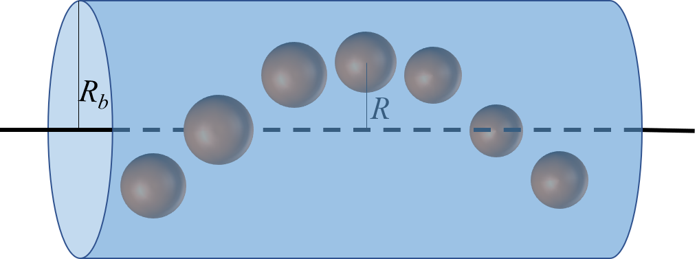
Figure 1: Illustration of the model, which consists of free electrons inside a cylindrical tube, containing a helical string of atomic-like scattering centers.

We use a model based on a helical string of atomic-like scattering potentials, sitting inside a perfectly straight wire, carrying Landauer-type conduction channels. The axis of the tube coincides with the $z$-axis in a system of cylindrical coordinates. Before introducing the localized scattering potentials, the conductance channels are those for a perfectly smooth and straight cylindrical free-electron-like conductor with hard-wall boundary conditions, and radius $R_{b}$ (Fig. 1). The eigenchannels for this perfect wire are given by,

$$\Psi_{\mu nk}(r,\varphi,z)=J_{\mu}(\gamma_{\mu n}r)e^{\mathfrak{i}kz}e^{\mathfrak{i}\mu\varphi}$$ (1)

Here, $\gamma_{\mu n}=x_{\mu n}/R_{b}$, with $x_{\mu n}$ the $n^{\rm th}$ zero of $J_{\mu}$, the $\mu^{\rm th}$ Bessel function ($n\geq 1$). The energy of this state is

$$\epsilon_{\mu nk}=\frac{\hbar^{2}}{2m}\gamma_{\mu n}^{2}+\frac{\hbar^{2}k^{2}}{2m}.$$ (2)

The interaction with the atomic-like spin-orbit terms is introduced as a perturbation of these states, by means of Fermi’s golden rule. Although the Coulomb potential of the atoms will be the dominant source of scattering, we propose to focus on the role of the spin-orbit interaction term only, and ignore potential scattering. Such a model could be a reasonable approximation for a metallic wire, where the electronic states are described by Bloch waves, containing a helical arrangement of heavy ions. At this point it is important to stress that we do not aim at a realistic description of a molecular wire. Yet, the model will help us to trace similar mechanisms in more realistic models. The advantage of having an explicit expression for the unperturbed states is that we may evaluate the matrix elements explicitly, which allows us to trace the origin of spin dependent scattering in our model.

For the spin-orbit interaction term we have,

$$\hat{h}_{0}=\frac{\mathfrak{i}\hbar^{2}}{4(mc)^{2}}\bm{\sigma}\left(\frac{\partial v(\mathbf{r})}{\partial\mathbf{r}}\times\bm{\nabla}\right).$$ (3)

Here, the differential operator $\partial/\partial_{\mathbf{r}}$ only acts on the electrostatic potential of the atomic nucleus, $v(\mathbf{r})$, while the operator $\bm{\nabla}$ on the right acts on the electron wave function. Although the cylindrical confining potential will also produce a contribution to the spin-orbit interaction, we will ignore this in the following, because the symmetry of this potential prohibits any back scattering. Forward scattering cannot lead to spin polarization, as we show in Section I.A.6, below.

The spin-flip rates induced by spin-orbit scattering are given by Fermi’s golden rule as,

$$\left.\frac{1}{\tau_{0}}\right|_{\mu nk\sigma}=2\pi\sum_{{\mu^{\prime}}\,{n^{\prime}}\,{k^{\prime}},{\sigma^{\prime}}} |\langle{\mu^{\prime}}{n^{\prime}}{k^{\prime}}{\sigma^{\prime}}|\hat{h}_{0}|\mu nk\sigma\rangle|^{2}\,\delta(E_{f}-E_{i}).$$ (4)

Here, $E_{i}=\epsilon_{\mu nk}$ and $E_{f}=\epsilon_{{\mu^{\prime}}{n^{\prime}}{k^{\prime}}}$ are the total energy of the initial and final states.

I.1 Evaluation of the matrix elements

I.1.1 Spin-orbit interaction in cylinder coordinates

In order to evaluate the matrix elements in (4) we need to work out the structure of the perturbing Hamiltonian (3). We express the spin operator $\bm{\sigma}$ in cylindrical coordinates as,

$$\bm{\sigma} =\sigma_{r}\bm{e}_{r}+\sigma_{\varphi}\bm{e}_{\varphi}+\sigma_{z}\bm{e}_{z}$$ (5)

$$=(e^{-\mathfrak{i}\varphi}\sigma_{+}+e^{+\mathfrak{i}\varphi}\sigma_{-})\bm{e}_{r}-\mathfrak{i}(e^{-\mathfrak{i}\varphi}\sigma_{+}-e^{+\mathfrak{i}\varphi}\sigma_{-})\bm{e}_{\varphi}+\sigma_{z}\bm{e}_{z},$$

where $\bm{e}_{r}$, $\bm{e}_{\varphi}$, and $\bm{e}_{z}$ are the unit vectors in cylindrical coordinates and,

$$\sigma_{+}=\hbar\begin{pmatrix}0&1\\ 0&0\end{pmatrix},\qquad\sigma_{-}=\hbar\begin{pmatrix}0&0\\ 1&0\end{pmatrix}=\sigma_{+}^{\dagger}.$$ (6)

Using coordinates $(r,\varphi,z)$ also for the electrons we can work out the vector products in the expression for $\hat{h}_{0}$ as,

$$\bm{\sigma}\left(\frac{\partial v(\mathbf{r})}{\partial\mathbf{r}}\times\bm{\nabla}\right)=\hat{h}_{z}\sigma_{z}+e^{-\mathfrak{i}\varphi}\hat{h}_{+}\sigma_{+}+e^{\mathfrak{i}\varphi}\hat{h}_{-}\sigma_{-}$$ (7)

where we have introduced the real-space operators

$$\hat{h}_{z}(r,\varphi,z) \coloneqq\frac{1}{r}\frac{\partial v}{\partial r}\frac{\partial}{\partial\varphi}-\frac{1}{r}\frac{\partial v}{\partial\varphi}\frac{\partial}{\partial r}$$

$$\hat{h}_{+}(r,\varphi,z) \coloneqq\frac{1}{r}\frac{\partial v}{\partial\varphi}\frac{\partial}{\partial z}-\frac{1}{r}\frac{\partial v}{\partial z}\frac{\partial}{\partial\varphi}-\frac{1}{\mathfrak{i}}\left(\frac{\partial v}{\partial r}\frac{\partial}{\partial z}-\frac{\partial v}{\partial z}\frac{\partial}{\partial r}\right)$$

and $\hat{h}_{-}\coloneqq\hat{h}_{+}^{*}$.

I.1.2 General structure of matrix elements

Due to (7), two kinds of matrix element appear in Eq. (4), spin flipping and non-flipping. The spin-conserving one is given by

$$\langle{\mu^{\prime}}{n^{\prime}}{k^{\prime}}{\sigma^{\prime}}|\hat{h}_{z}\sigma_{z}|\mu nk\sigma\rangle=\langle{\mu^{\prime}}{n^{\prime}}{k^{\prime}}|\hat{h}_{z}|\mu nk\rangle\langle{\sigma^{\prime}}|\sigma_{z}|\sigma\rangle$$ (8)

The second matrix element on the rhs is trivially evaluated as

$$\langle{\sigma^{\prime}}|\sigma_{z}|\sigma\rangle=\text{sign}({\sigma})\delta_{{\sigma^{\prime}}\sigma},$$ (9)

while the first matrix element on the rhs of (8) takes the explicit form

$$I_{z}^{{\mu^{\prime}}{n^{\prime}}{k^{\prime}},\mu nk}=\int_{0}^{R_{b}} dr\int_{-\infty}^{+\infty}dz\int_{0}^{2\pi}rd\varphi\ e^{-\mathfrak{i}{\mu^{\prime}}\varphi}\ e^{-\mathfrak{i}{k^{\prime}}z}$$

$$\times J_{{\mu^{\prime}}}(\gamma_{{\mu^{\prime}}{n^{\prime}}}r)\ \hat{h}_{z}(r,\varphi,z)\ e^{\mathfrak{i}\mu\varphi}\ e^{\mathfrak{i}kz}J_{\mu}(\gamma_{\mu n}r).$$ (10)

The spin-non-conserving matrix elements are given by

$$\langle{\mu^{\prime}}{n^{\prime}}{k^{\prime}}{\sigma^{\prime}}| e^{\mp\mathfrak{i}\varphi}\hat{h}_{\pm}\sigma_{\pm}|\mu nk\sigma\rangle=$$

$$\langle{\mu^{\prime}}{n^{\prime}}{k^{\prime}}|e^{\mp\mathfrak{i}\varphi}\hat{h}_{\pm}|\mu nk\rangle\langle{\sigma^{\prime}}|\sigma_{\pm}|\sigma\rangle$$ (11)

The second matrix element on the rhs for $\sigma_{+}$ and $\sigma_{-}$ is non-vanishing only for $\sigma=\downarrow$ and $\sigma=\uparrow$, respectively:

$$\langle{\sigma^{\prime}}|\sigma_{+}|\sigma\rangle =\delta_{{\sigma^{\prime}}\uparrow}\delta_{\sigma\downarrow},$$

$$\langle{\sigma^{\prime}}|\sigma_{-}|\sigma\rangle =\delta_{{\sigma^{\prime}}\downarrow}\delta_{\sigma\uparrow},$$ (12)

while the first matrix element takes the explicit form

$$I_{\pm}^{{\mu^{\prime}}{n^{\prime}}{k^{\prime}},\mu nk}=\int_{0}^{R_{b}} dr\int_{-\infty}^{+\infty}dz\int_{0}^{2\pi}rd\varphi\ e^{-\mathfrak{i}({\mu^{\prime}}\pm 1)\varphi}\ e^{-\mathfrak{i}{k^{\prime}}z}$$

$$\times J_{{\mu^{\prime}}}(\gamma_{{\mu^{\prime}}{n^{\prime}}}r)\ \hat{h}_{\pm}(r,\varphi,z)\ e^{\mathfrak{i}\mu\varphi}\ e^{\mathfrak{i}kz}\ J_{\mu}(\gamma_{\mu n}r).$$ (13)

Based on these expressions we introduce rates for spin-conserving and spin-flipping processes

$$\left.\frac{1}{\tau_{z}}\right|_{\mu nk\sigma}{=}2\pi\xi^{2}\sum_{{\mu^{\prime}}\,{n^{\prime}}\,{k^{\prime}}} |I^{{\mu^{\prime}}{n^{\prime}}{k^{\prime}},\mu nk}_{z}|^{2}\delta(E_{f}-E_{i})$$

$$\left.\frac{1}{\tau_{+}}\right|_{\mu nk\downarrow}{=}2\pi\xi^{2}\sum_{{\mu^{\prime}}\,{n^{\prime}}\,{k^{\prime}}} |I^{{\mu^{\prime}}{n^{\prime}}{k^{\prime}},\mu nk}_{+}|^{2}\delta(E_{f}{-}E_{i})$$

$$\left.\frac{1}{\tau_{-}}\right|_{\mu nk\uparrow}{=}2\pi\xi^{2}\sum_{{\mu^{\prime}}\,{n^{\prime}}\,{k^{\prime}}} |I^{{\mu^{\prime}}{n^{\prime}}{k^{\prime}},\mu nk}_{-}|^{2}\delta(E_{f}{-}E_{i}),$$ (14)

with $\xi=\hbar^{2}/(4m^{2}c^{2})$. These three scattering rates follow directly from the three terms in Eq. (7), and can be considered separately because the processes do not mutually interfere. The most interesting situations arise when the rates for up- or down-conversion of the spins, i.e. the lower two lines of (14), differ.

I.1.3 Evaluation of the integrals

The integral for the spatial coordinates in (10) has two terms inherited from the structure of $\hat{h}_{z}$. The partial derivative $\frac{\partial}{\partial\varphi}$ at the right in the operator $\hat{h}_{z}$, acting on a wave function $|\mu nk\sigma\rangle$, produces $\mathfrak{i}\mu$. The two terms can be combined through partial integration. For the first term we use for the integral over $r$,

$$\mathfrak{i}\mu\int_{0}^{R_{b}} \,\frac{\partial v}{\partial r}\,J_{{\mu^{\prime}}}J_{\mu}\,dr=$$ (15)

$$-\mathfrak{i}\mu\int_{0}^{R_{b}}\,v\,\left(J_{\mu}\frac{dJ_{{\mu^{\prime}}}}{dr}+J_{{\mu^{\prime}}}\frac{dJ_{\mu}}{dr}\right)\,dr.$$

where we write $J_{\mu}$ and $J_{{\mu^{\prime}}}$ as short for $J_{\mu}(\gamma_{\mu n}r)$ and $J_{{\mu^{\prime}}}(\gamma_{{\mu^{\prime}}{n^{\prime}}}r)$.

For the second term we use,

$$\int_{0}^{2\pi}\,e^{-\mathfrak{i}(\mu-{\mu^{\prime}})\varphi}\frac{\partial v}{\partial\varphi}\, d\varphi=$$ (16)

$$-\mathfrak{i}(\mu-{\mu^{\prime}})\int_{0}^{2\pi}v\,e^{-\mathfrak{i}(\mu-{\mu^{\prime}})}\,d\varphi.$$

The two terms combine into,

$$I_{z}^{{\mu^{\prime}}{n^{\prime}}{k^{\prime}},\mu nk} =-\mathfrak{i}\int_{0}^{R_{b}}dr\int_{-\infty}^{+\infty}dz\,\int_{0}^{2\pi}d\varphi\ \,v(\mathbf{r})\,e^{\mathfrak{i}(\mu-{\mu^{\prime}})\varphi}$$

$$\times e^{\mathfrak{i}(k-{k^{\prime}})z}\,\left(\mu J_{\mu}\frac{dJ_{{\mu^{\prime}}}}{dr}+{\mu^{\prime}}J_{{\mu^{\prime}}}\frac{dJ_{\mu}}{dr}\right)$$ (17)

By similar steps we obtain for the corresponding integrals for the operators $\hat{h}_{\pm}$,

$$I_{\pm}^{{\mu^{\prime}}{n^{\prime}}{k^{\prime}},\mu nk} =\int_{0}^{R_{b}}dr\int_{-\infty}^{+\infty}dz\int_{0}^{2\pi}d\varphi\,v(\mathbf{r})\,e^{\mathfrak{i}(\mu-{\mu^{\prime}}\mp 1)\varphi}\times$$

$$e^{\mathfrak{i}(k-{k^{\prime}})z} \left[(\mu{k^{\prime}}-{\mu^{\prime}}k)J_{{\mu^{\prime}}}J_{\mu}\pm r\left(kJ_{\mu}\frac{dJ_{{\mu^{\prime}}}}{dr}+{k^{\prime}}J_{{\mu^{\prime}}}\frac{dJ_{\mu}}{dr}\right)\right].$$ (18)

Here, we have assumed that the potential $v(\mathbf{r})$ vanishes for $z\rightarrow\pm\infty$, but otherwise it has not yet been specified.

I.1.4 Limiting case: a single ‘atom’

Note that the potential due to a single atomic-like scatterer does not define a chiral structure. Yet, we find a difference between the integrals for $\tau_{+}$ and $\tau_{-}$ in (I.1.3) even for a single scattering center. This spin-dependent scattering arises from the combination of the finite orbital angular momentum $\hbar\mu$ and $\hbar{\mu^{\prime}}$ of the incoming and scattered waves, in combination with the off-axis position of the ‘atom’. Experiments that permit selection of the angular momentum of incoming waves may observe this spin-dependent scattering, but typical experiments select the incoming waves by energy only.

This chiral effect that is not associated with a chiral potential is removed by summation of contributions of all incoming electrons at the same energy. This can be seen from the fact that $I_{+}^{{\mu^{\prime}}{n^{\prime}}{k^{\prime}},\mu nk}=-I_{-}^{-{\mu^{\prime}}{n^{\prime}}{k^{\prime}},-\mu nk}$, so that $|I_{+}^{{\mu^{\prime}}{n^{\prime}}{k^{\prime}},\mu nk}|^{2}=|I_{-}^{-{\mu^{\prime}}{n^{\prime}}{k^{\prime}},-\mu nk}|^{2}$. Therefore, for a single ‘atom’,

$$\left.\frac{1}{\tau_{+}}\right|_{\mu nk\downarrow}=\left.\frac{1}{\tau_{-}}\right|_{-\mu nk\uparrow}$$ (19)

Since the states with quantum number $\mu$ are degenerate with those having $-\mu$ we should consider the sum of the scattering rates for $\mu$ and $-\mu$ and, thus, this sum is equal for $\tau_{+}$ and $\tau_{-}$.

Concluding, as we should expect, a single atomic-like potential does not represent a chiral structure and only produces spin-dependent scattering when we can conceive of an experiment that selects the orbital states of the electron waves. Below we will combine the scattering of a string of ‘atoms’ and demonstrate that spin dependence results from a helical arrangement of single scatterers.

The potential $v(\mathbf{r})$ in (3) describes the electrostatic potential due to the ‘atoms’ inside the tube. As a first step, we limit this to a single site at $(R,\Phi,Z)$. We calculate the matrix elements explicitly by adopting a minimal model for the scattering potential $v(\mathbf{r})$. The potential is normally given by the Coulomb interaction between the electrons and the effective core. For the purpose of the minimal model we have the freedom of adjusting the actual form of this potential, and for computational convenience we choose it to be a delta function

$$v(r,\varphi,z)=K_{0}\delta(r-R)\frac{1}{r}\delta(\varphi-\Phi)\delta(z-Z).$$ (20)

With this, the integrals for the spatial coordinates in matrix elements for $\hat{h}_{z}$, $\hat{h}_{+}$ and $\hat{h}_{-}$ become,

$$\quad I_{z}^{{\mu^{\prime}}{n^{\prime}}{k^{\prime}},\mu nk}=-\mathfrak{i}K_{0}e^{\mathfrak{i}(\mu-{\mu^{\prime}})\Phi}e^{\mathfrak{i}(k-{k^{\prime}})Z}\times$$ (21)

$$\qquad\qquad\left[\frac{1}{r}\left(\mu J_{\mu}\frac{dJ_{{\mu^{\prime}}}}{dr}+{\mu^{\prime}}J_{{\mu^{\prime}}}\frac{dJ_{\mu}}{dr}\right)\right]_{r=R},$$

$$\quad I_{\pm}^{{\mu^{\prime}}{n^{\prime}}{k^{\prime}},\mu nk}=K_{0}e^{\mathfrak{i}(\mu-{\mu^{\prime}}\mp 1)\Phi}e^{\mathfrak{i}(k-{k^{\prime}})Z}\times$$

$$\qquad\left[\frac{1}{r}(\mu{k^{\prime}}-{\mu^{\prime}}k)J_{\mu}J_{{\mu^{\prime}}}\pm\left(kJ_{\mu}\frac{dJ_{{\mu^{\prime}}}}{dr}+{k^{\prime}}J_{{\mu^{\prime}}}\frac{dJ_{\mu}}{dr}\right)\right]_{r=R}.$$

The terms in square brackets depend on the quantum numbers, but otherwise only on the radial distance $R$ for the position of the atomic potential. The dependence on $Z$ and $\Phi$ is completely covered by the phase factors in the first lines of (21).

I.1.5 A helical string of atomic-like scatterers

In order to implement a chiral structure we arrange $2N+1$ identical ‘atoms’ along a helix inside the cylindrical conductor at positions $(R,\nu\theta,\nu s)$ for $\nu=-N,\ldots,N$, where the constants $\theta$ and $s$ describe the chirality of the ‘molecule’. Thus, we write the potential $v$ in the form of a sum over the potentials of the individual nuclei,

$$v_{N}(\mathbf{r})=\sum_{\nu=-N}^{N}v_{0}(r-R,\,\varphi-\nu\theta,\,z-\nu s),$$ (22)

where $v_{0}$ is the potential due to a single scattering center.

In order to evaluate the matrix elements for this potential, we insert it in Eqs. (I.1.3) and (I.1.3). The scattering amplitudes from each of the ‘atoms’ in the string receive phase factors according to (21), which allows us to express the integrals as,

$$I_{z}^{{\mu^{\prime}}{n^{\prime}}{k^{\prime}},\mu nk} =I_{z}^{{\mu^{\prime}}{n^{\prime}}{k^{\prime}},\mu nk}(v_{0})\sum_{\nu=-N}^{N}e^{\mathfrak{i}\nu(s\Delta k+\theta\Delta\mu)}$$

$$= I_{z}^{{\mu^{\prime}}{n^{\prime}}{k^{\prime}},\mu nk}(v_{0})\quad\frac{\sin{((N+\tfrac{1}{2})(s\Delta k+\theta\Delta\mu))}}{\sin{(\tfrac{1}{2}(s\Delta k+\theta\Delta\mu))}}$$

$$I_{\pm}^{{\mu^{\prime}}{n^{\prime}}{k^{\prime}},\mu nk} =I_{\pm}^{{\mu^{\prime}}{n^{\prime}}{k^{\prime}},\mu nk}(v_{0})\sum_{\nu=-N}^{N}e^{\mathfrak{i}\nu(s\Delta k+\theta(\Delta\mu\mp 1))}$$

$$=I_{\pm}^{{\mu^{\prime}}{n^{\prime}}{k^{\prime}},\mu nk} (v_{0})\quad\frac{\sin{((N+\tfrac{1}{2})(s\Delta k+\theta(\Delta\mu\mp 1)))}}{\sin{(\tfrac{1}{2}(s\Delta k+\theta(\Delta\mu\mp 1)))}},$$ (23)

where $\Delta k={k^{\prime}}-k$ and $\Delta\mu=\mu-{\mu^{\prime}}$. The integrals on the rhs are evaluated for the potential $v_{0}$ due to a single scattering center. The sums in (I.1.5) generally lead to near-cancellations, unless the argument $s({k^{\prime}}-k)+\theta(\mu-{\mu^{\prime}}\mp 1)$ is close to a multiple of $2\pi$. This quantum interference effect strongly selects specific channels for spin scattering.

This is the central result of this paper: quantum interference breaks the symmetry between spin-up and spin-down scattering. For example, consider initial and final states with ${\mu^{\prime}}=\mu$ and ${n^{\prime}}=n$. Energy conservation requires ${k^{\prime}}=\pm k$. For back scattering we have ${k^{\prime}}=-k$, so that the arguments are $x=-2ks-\theta$ for $I_{+}$ and $x=-2ks+\theta$ for $I_{-}$. This breaks the symmetry of (19), in particular for the energy range for which $k\simeq\theta/2s$ so that $x$ approaches zero for $I_{-}$, while $x\simeq 2\theta$ for $I_{+}$, which will be typically far from zero. The other spin channel is selected when $x=-2ks-\theta\simeq-2\pi$.

At higher energy many combinations of quantum numbers lead to constructive interference, and in order to evaluate this we need to resort to numerical evaluation of the expressions.

I.1.6 Absence of spin-dependent forward scattering

In order to suppress scattering that is not associated with the chiral shape of the potential we consider the average of scattering of all states available at a given energy,

$$\left.\frac{1}{\tau_{\pm}}\right|_{E}{=}\frac{1}{n_{\tau}}\sum_{\mu\,n}\sum_{k>0}\left.\frac{1}{\tau_{\pm}}\right|_{\mu nk\sigma}\delta(E-\epsilon_{\mu nk}),$$ (24)

where the energy for each of the states $\epsilon_{\mu nk}$ is given by (2), and $n_{\tau}$ counts the numbers of states available at this energy. The polarization of the spin scattering can then be defined as,

$$P(E)=\frac{\left.\frac{1}{\tau_{+}}\right|_{E}-\left.\frac{1}{\tau_{-}}\right|_{E}}{\left.\frac{1}{\tau_{+}}\right|_{E}+\left.\frac{1}{\tau_{-}}\right|_{E}+\left.\frac{1}{\tau_{z}}\right|_{E}}$$ (25)

Remarkably, we find that the polarization for forward scattering (${k^{\prime}}>0$) is identical to zero. In order to demonstrate this let us consider incoming states with energy $E$ and quantum numbers $\mu,n,k>0$. The spin-flip scattering rates averaged over states at energy $E$ can be written as,

$$\left.\frac{1}{\tau_{+}}\right|_{E}^{\text{fwd.}} =\frac{2\pi\xi^{2}}{n_{\tau}}\,\sum_{\mu nk}\sum_{{\mu^{\prime}}{n^{\prime}}{k^{\prime}}}\ \left|\bra{{\mu^{\prime}}{n^{\prime}}{k^{\prime}}\downarrow}\,\hat{h}_{0}\,\ket{\mu nk\uparrow}\right|^{2}$$

$$\qquad\qquad\times\delta(E-\epsilon_{\mu^{\prime}n^{\prime}k^{\prime}})\delta(E-\epsilon_{\mu nk})$$ (26a)

$$\left.\frac{1}{\tau_{-}}\right|_{E}^{\text{fwd.}} =\frac{2\pi\xi^{2}}{n_{\tau}}\,\sum_{\mu nk}\sum_{{\mu^{\prime}}{n^{\prime}}{k^{\prime}}}\ \left|\bra{{\mu^{\prime}}{n^{\prime}}{k^{\prime}}\uparrow}\,\hat{h}_{0}\,\ket{\mu nk\downarrow}\right|^{2}$$

$$\qquad\qquad\times\delta(E-\epsilon_{\mu^{\prime}n^{\prime}k^{\prime}})\delta(E-\epsilon_{\mu nk}).$$ (26b)

In order to account for forward scattering only we restrict the final-state momenta to positive values, $k^{\prime}>0$. In this case, the indices $\mu,n,k$ and ${\mu^{\prime}},{n^{\prime}},{k^{\prime}}$ run through identical sets of quantum numbers in the (26). When one uses the fact that $\hat{h}_{0}$ in (26) is hermitian, and relabels the indices, it it easy to see that

$$\left.\frac{\hbar}{\tau_{+}}\right|_{E}^{\text{fwd.}}=\left.\frac{\hbar}{\tau_{-}}\right|_{E}^{\text{fwd.}}.$$ (27)

This identity does not apply for back scattering, because in this case the summation over $k$ and ${k^{\prime}}$ cannot be interchanged. In the following we will focus on the properties of back scattered electron spins.

II Numerical evaluation

The many contributions to the sums in (14) require numerical evaluation. For back scattering we find the result plotted in Fig. 2. The important result we obtain is that $P(E)$ is typically large, and even approaches complete polarization in some regions of energy. When we change the sign of the chirality (by $s\rightarrow-s$, or $\theta\rightarrow-\theta$) the graph is reflected around the horizontal axis, as expected. We find that the spin-conserving term $1/\tau_{z}$ only makes a minor contribution to the total scattering rates.

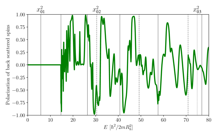
Figure 2: Constructive interference of the spin scattering in a string of 21 ‘atoms’ (N=10). Here $P$ is the ratio of the rates for back scattering spins from up to down and the reverse process, as given by Eq. (25), as a function of energy $E$, in units $\hbar^{2}/(2mR_{b}^{2})$. The angle between successive scattering centers in the helical string is set at $\theta=2\pi/10$, and the distance between the sites $s=0.85$ in units of $R_{b}$. The vertical lines mark the points of opening of new conductance channels for $n=1$ (solid), $n=2$ (dashed), and $n=3$ (dotted). Successive lines in the same style have increasing values of $\mu$. Changing the sign of the chirality produces a curve with the opposite sign.

Initially, $P(E)$ is zero, because below $(\gamma_{01}/R_{b})^{2}=5.78$ there are no conduction channels available. After that point the first channel opens, with $\mu=0,\,n=1$, ${\mu^{\prime}}=0,\,{n^{\prime}}=1$, and this remains the only channel until $(\gamma_{11}/R_{b})^{2}=14.68$. In this range of energies the transmission and reflection of spins is exactly balanced, in accordance with Kramers’ degeneracy for a single-channel conductor.Bardarson (2008) In our expressions, this absence of spin scattering for the lowest conductance channel can be read from (21): the first term in the square brackets vanishes for $\mu={\mu^{\prime}}=0$, and the second term cancels because the Bessel functions for $\mu$ and ${\mu^{\prime}}$ are the same, and because ${k^{\prime}}=-k$ for back scattering into the same channel.

Once we cross $E=14.68$ additional conductance channels become accessible, having non-zero angular momentum quantum numbers $\mu,\,{\mu^{\prime}}=\pm 1$, with $n={n^{\prime}}=1$. The contributions of these channels allow for the integrals (21) to become finite, and the gradual increase of $k$ and ${k^{\prime}}$ above $E=14.68$ leads to rapid oscillations of $P(E)$ due to the phase factors in (I.1.5). The polarization continues to fluctuate with energy, but longer-period components take over. In some cases it is possible to trace the saturation of $P$ near 1 to a contribution for which the argument of the phase factor in the interference $x=s(k-{k^{\prime}})+\theta(\mu-{\mu^{\prime}}\pm 1)$ becomes very small, so that all terms add constructively. When this happens the spin scattering rate for these terms shows a very long period oscillation as a function of energy and as a function of the numbers of ‘atoms’ in the string.

Importantly, we find that $P(E)$ maintains predominantly the same sign over wide ranges of energy. For example, $P$ is almost exclusively positive between $E=17.5$ and $E=27.5$. Since many experiments do not select a sharply defined energy, but a finite range of energies contributes to the signal, it is useful to integrate the scattering rates over an energy window.

Figure 3 shows the rates $\left.1/\tau_{+}\right|_{E}$ (red), $\left.1/\tau_{-}\right|_{E}$ (blue), and $\left.1/\tau_{z}\right|_{E}$ (green) for $2N+1=41$ atomic scattering centers, integrated from E = 17.5 to E. Clearly the difference between the two spin scattering directions is large, in particular at the lower energy end. At higher energies the predominance of spin-up vs. spin-down scattering alternates.

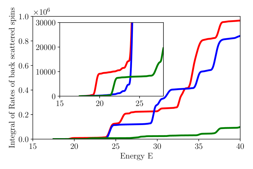
Figure 3: Rates $\left.1/\tau_{+}\right|_{E}$ (red), $\left.1/\tau_{-}\right|_{E}$ (blue), and $\left.1/\tau_{z}\right|_{E}$ (green) integrated over energy from $E=17.5$, for $2N+1=41$. The rates are given in arbitrary units. The inset shows the low-energy range on an expanded scale.

One of the hallmark observations in the experiments is a roughly linear dependence of the spin polarization with the length of the molecule. In our model, at any given energy we find that the scattering rates oscillate with the number of ‘atoms’ $2N+1$ included in the helical string. This oscillation is often rapid, but long-period oscillations are found near the points where $P(E)$ approaches 1 or -1 (Fig. 2). However, as noted above, experiments typically measure the signals due to a finite range of energies. Figure 4 shows the two spin scattering rates, integrated from $E=17.5$ to $E=27.5$, as a function of the length of the helical string, where the number of atoms is $2N+1$. The observed dependence is close to linear, while the polarization $P$ remains approximately constant. The linear dependence of the spin scattering rates persists (at least up to $N=100$), so that the spin scattering can, in principle, dominate other sources of scattering for long molecules. The linear dependence will ultimately saturate due to interactions that are not included in our model, such as multiple scattering and inelastic scattering.

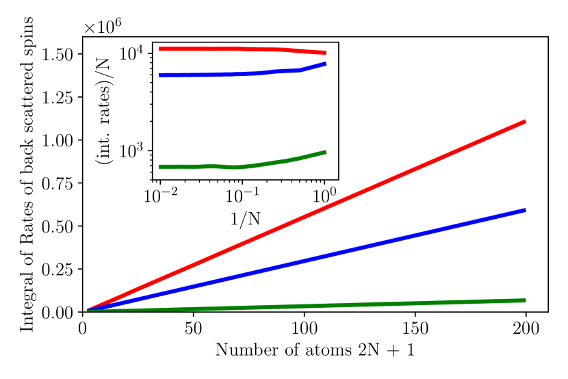
Figure 4: Energy-integrated back scattering rates $\left.1/\tau_{+}\right|_{E}$ (red), $\left.1/\tau_{-}\right|_{E}$ (blue), and $\left.1/\tau_{z}\right|_{E}$ (green) as a function of the length of the helical string. The integration over energy is taken from $E=17.5$ to $E=27.5$. The number of atoms in the string is $2N+1$. At $N=0$ the tube contains one atom, and the blue and red rates are equal, as expected. The inset plots the rates devided by $N$, as a function of $1/N$, which demonstrates the saturation to a constant slope of the rates for large $N$. The rates are given in arbitrary units.

III Discussion and conclusion

The model presented above was investigated in order to trace a possible origin of the chirality-induced spin selectivity. We find that quantum interference of partial waves scattered off atomic spin-orbit interactions leads to selective back scattering of one spin component over the other. Although this mechanism appears to be intuitively appealing, we cannot claim that we offer a quantitative explanation of the CISS effect. The nature of the unperturbed electronic states is idealized in our model, and the spin-orbit interaction at the atomic sites is represented by a delta-function potential, which is clearly not realistic. Therefore, the quantitative outcomes for the scattering rates cannot be taken literally for a comparison with experiments.

The strong points of the mechanism proposed here is that it is robust, conceptually simple, and may be applicable to a wider range of unperturbed molecular wave functions. In our model, spin selectivity is found in wide ranges of energy, despite the smallness of the spin-orbit interaction. This contrasts with the model proposed by Michaeli,Michaeli and Naaman (2019) which produces spin selectivity of order unity only in a narrow window of a few meV at low energies. In our case it is found for all energies above a certain threshold value. Furthermore, we find that the spin scattering rates increase almost linearly with the length of the ’molecule’, in agreement with observations.Göhler et al. (2011)

An interesting feature of our model is that the sign of the spin scattering is not uniquely determined by the handedness, as shown by the plot in Fig. 2, but also by the helicity $\theta/s$ and by the energy range that we consider. Most experiments have compared the effects of the sign of chirality by comparing the two enantiomers, or have studied similar molecular structures as a function of length, all under the same experimental conditions. In a system that can be described by this quantum interference mechanism one would expect to observe sign changes when varying the helical pitch, even when maintaining the same sign of chirality, or when probing the system in a different energy range.

The model considered here is consistent with Landauer’s picture of a phase-coherent scattering problem. It transitions to a classical resistance only when we add inelastic scattering to the description, and consider the limit of very long helical wires. Even at room temperature, for most chiral molecules probed in experiments the inelastic scattering length is much longer than the length of the molecule. On the other hand, the long DNA strands tested by Gohler et al.Göhler et al. (2011) are possibly long enough for temperature-induced dephasing to become observable.

In conclusion, we propose a simple model of constructive quantum interference as a mechanism giving rise to spin-selective electron reflection. The mechanism proposed here may guide the design of experiments and the analysis of more realistic computations. We have limited our discussions to possible explanations of spin-selectivity in the transmission properties of chiral molecules, and the model presented here offers a simple and intuitive mechanism that may be transferable to actual molecular systems. We have refrained from touching upon experiments that involve charge detection, rather than spin directly, because of the additional complications involved in describing the spin-to-charge conversion (both in terms of the modeling, and regarding the proper design of the experimental conditions). The observation of the third class of experiments, revolving around near-equilibrium properties of enantiomer absorption on magnetized surfaces, pose even greater difficulties for explanation, and we have not attempted at addressing those. A proper understanding of spin-selective transmission may form a solid basis for proceeding with developing an explanation for the second two classes of experiments.