COVID-19 incidence in the Republic of Ireland: A case study for network-based time series models

Abstract

Network-based Time Series models have experienced a surge in popularity over the past years due to their ability to model temporal and spatial dependencies such as arising from the spread of an infectious disease. As statistical models for network time series, generalised network autoregressive (GNAR) models have been introduced. GNAR models are vertex-based models which have an autoregressive component modelling temporal dependence and a spatial autoregressive component to incorporate dependence between neighbouring vertices in the network.

This paper compares the performance of GNAR models with different underlying networks in predicting COVID-19 cases for the 26 counties in the Republic of Ireland. The dataset is separated into subsets according to inter-country movement regulations and categorized into two pandemic phases, restricted and unrestricted. Ten static networks are constructed based on either general or COVID-19 specific approaches. In these networks, vertices represent counties, and edges are built upon neighbourhood relations, such as railway lines.

We find that while for the prediction task, no underlying static network is consistently superior for either restricted or unrestricted phase, for pandemic phases with restrictions sparse networks perform better while for unrestricted phases, dense networks explain the data better. GNAR models have higher predictive accuracy than ARIMA models, which ignore the network structure. ARIMA and GNAR models perform similarly in pandemic phases with more lenient or no COVID-19 regulation. These findings indicate evidence of network dependencies in the restricted phase, but not in the unrestricted phase. They also show some robustness regarding the network construction method. An analysis of the residuals justifies the model assumptions for the restricted phase but raises questions for the unrestricted phase.

2020 Mathematics Subject Classification: 62M10, 05C82, 91D30 Network-based time series, COVID-19, spatial models, networks

1 Introduction

In recent years, statistical models which incorporate networks and thereby acknowledge spatial dependencies when predicting temporal data have experienced a surge in popularity (e.g.  [1, 2, 3]). Against this backdrop, Knight et al. [2] developed a generalised network autoregressive (GNAR) time series model which in addition to the standard temporal dependence when modelling time series data, also incorporates a second type of dependence; this dependence is captured in a network. In [2] the proposed network-based time series model is leveraged to predict mumps incidence across English counties during the British mumps outbreak in 2005.
Similar to mumps, COVID-19 is a highly infectious disease spread by direct contact between people [4]. Human movement networks have been extensively relied upon to explain COVID-19 patterns (e.g. [5, 6, 7, 8, 4, 9, 10]). Therefore, it is a natural conjecture that such movement networks may help predict the spread of COVID-19. This paper

• fits GNAR models to predict the weekly COVID-19 incidence for all 26 counties in the Republic of Ireland, exploring different network constructions;

• assesses the prevalence of a network effect in COVID-19 incidence in Ireland and the suitability of GNAR models to predict epidemic outbreaks as complex as COVID-19;

• investigates the influence of changes in inter-county mobility, due to COVID-19 restrictions, on the performance of GNAR models as well as on the model parameters and hyperparameters.

The networks are constructed according to general approaches based on statistical definitions of neighbourhoods as well as approaches specific to the infectious spread of the COVID-19 virus. For each network, for prediction with the GNAR model we select the best performing hyperparameter values using the Bayesian Information Criterion. By splitting the available Irish data into two phases of the pandemic, restricted and unrestricted, we are able to investigate the potential change in the temporal and spatial dependencies in COVID-19 incidence between the two phases.

This paper is organised as follows. Section 2 introduces the data set. The methodology for network construction and for network-based time series modeling is described in Section 3. Section 4 provides an exploratory data analysis, while the model fit is shown in Section 5.1. The conclusions for the different pandemic phases are found in Section 5.2. The results are discussed in Section 6; concluding remarks are provided in Section 7. The extensive Supplementary Material include the history of the COVID-19 outbreak in Ireland as well as additional material, visualising the COVID-19 data as well as the constructed networks, and illustrating the performance of the network-based time series models on the COVID-19 networks.

The code as well as the original and processed data for the paper is available on GitHub: https://github.com/stephanieArmbru/Case_study_GNAR_COVID_Ireland.git.

2 The Irish COVID-19 data set

By March 2023, the Republic of Ireland had recorded a total of 1.7 million confirmed COVID-19 cases and 8,719 deaths [11] since the beginning of the pandemic. In this paper, from now on we abbreviate the Republic of Ireland by Ireland. The Health Protection Surveillance Centre identified four main variants of concern for the COVID-19 virus in Ireland [12], in addition to the original variant: Alpha from 27.12.2020, Delta from 06.06.2021, Omicron I from 13.12.2021, and Omicron II from 13.03.2022 (Figure 1a in [12]). The open data platform [13, 14] by the Irish Government provides weekly updated multivariate time series data on confirmed daily cumulative COVID-19 cases for all 26 Irish counties, starting from the beginning of the pandemic in February 2020. A COVID-19 case is attributed to the county the patient has their primary residence in . The cumulative case count is given for 100,000 inhabitants and population corrected according to the population size from the 2016 census of Ireland [15].

In the data used this paper, the first COVID-19 case was registered in Dublin on 02.03.2020 and the last reported date is 23.01.2023, spanning a total of 152 weeks [14]. From 20.03.2020 onward, patients were suffering from COVID-19 in every Irish county. The daily COVID-19 data is aggregated to a weekly level to avoid modelling artificial weekly effects [16, 17]. Due to delayed reporting during winter 2021/22, the weekly COVID-19 incidences from 12.12.2021 to 27.02.2022 are averaged over a window of 4 weeks [18, 19, 20].

The main COVID-19 regulations restricting physical movement and social interaction between Irish counties [21, 22, 23, 24] are leveraged to naturally split the data into five subsets. The standard deviation in COVID-19 incidence across the 16 Irish counties, averaged over the considered time period, is indicated by $\bar{\sigma}$.

1. Start of the pandemic, with gradually stricter movement restrictions and lockdowns (restricted phase), from 27.02.2020 for 25 weeks ($\bar{\sigma}=19.17$);

2. County-specific movement restrictions (less restricted phase), from 18.08.2020 for 18 weeks ($\bar{\sigma}=35.05$);

3. Level-5 lockdown (restricted phase), with inter-county travel restrictions, from 26.12.2020 for 20 weeks ($\bar{\sigma}=148.79$);

4. Allowance of non-essential inter-county travel (less restricted phase), from 10.05.2021 for 43 weeks ($\bar{\sigma}=173.17$);

5. End of all restrictions (unrestricted phase), from 06.03.2022 for 46 weeks ($\bar{\sigma}=101.46$).

When split according to major movement restrictions, the individual data subsets have too few observations to train GNAR models and assess their prediction accuracy. Hence, the datasets are grouped as follows. Datasets 1 and 3 are concatenated, representing pandemic situations with strict COVID-19 restrictions, including an inter-county travel ban [21]; we call this the restricted data set. The restricted dataset contains 45 weeks of observation (average standard deviation across time period and counties $\sigma_{r}=99.27$). Datasets 2, 4 and 5 represent periods with fewer or no regulations, in particular no inter-county travel limitations [24]. We concatenate these data set to give the unrestricted data set. It has 107 weeks of observation (average standard deviation across time period and counties $\sigma_{ur}=129.62$). For the concatenation, the time gaps are inserted as missing data, 23.08.2020 - 20.12.2020 for the restricted dataset, and 27.12.2020 - 09.05.2021 for the unrestricted dataset.

3 Methodology

We first fix some notation. Throughout this paper, $\mathcal{G}=\{\mathcal{V},\mathcal{E}\}$ is a deterministic undirected network with vertex set $\mathcal{V}$ containing $N$ vertices and edge set $\mathcal{E}$; an edge between vertices $i$ and $j$ is denoted by $i\sim j$. All networks are unweighted and simple, without multiple edges and without self-loops. The neighbourhood of a subset of vertices $A\subset\mathcal{V}$ is defined as the set of neighbours outside of $A$ to the vertices in $A$,

$$N(A)=\bigcup_{i\in A}\{j\in\mathcal{V}\backslash A:i\sim j\}.$$

The set of $r^{\,th}$-stage neighbours, or the $r^{\,th}$-stage neighbourhood, for vertex $i\in A$ is defined recursively as $N^{(0)}(i)=\{i\}$ and

$$N^{(r)}(i)=N\left(N^{(r-1)}(i)\right)\backslash\bigcup_{q=1}^{r-1}N^{(q)}(i)\;.$$

3.1 COVID-19 networks: constructions and properties

COVID-19 specific networks can be constructed intuitively, leveraging that human mobility has a shaping influence on disease spread ([25, 5, 7, 8, 9] ). Hence our first set of networks are based on geographical approaches, as follows.

In the Railway-based network, an edge is established between two counties if there exists a direct train link between the respective county towns (without change of trains) and the county towns are closest to each other on this train connection. The Queen’s contiguity network connects each county with the counties it shares a border with [26]. The Economic hub network adds an additional edge between each county and its nearest economic hub, Dublin, Cork, Limerick, Galway or Waterford, to the Queen’s contiguity network. . To measure the distance to the nearest economic hub we use the Great Circle distance $d_{C}({i,j})$, the shortest distance between two points on the surface of a sphere [28]. For two points $i,j$ with latitude $\delta_{i},\delta_{j}$ and longitude $\lambda_{i},\lambda_{j}$ on a sphere of radius $r>0$,

$$d_{C}(i,j) =r\cdot cos^{-1}\left(cos(\delta_{i})\cdot cos(\delta_{j})\cdot cos(\lambda_{i}-\lambda_{j})-sin(\delta_{i})\cdot cos(\delta_{j})\right)\;.$$

The K-nearest neighbours network (KNN) connects a vertex with its $K$ nearest neighbours with respect to $d_{C}$ [29, 30]. The distance-based-nearest-neighbour network (DNN) constructs an edge between counties if their Great Circle distance $d_{C}$ lies within a certain range $[l,r]$ [28]. For the COVID-19 network, we set $l=0$ and consider $r$ a hyperparameter, chosen large enough to ensure that no vertex is isolated. The maximum value for $r$ is determined by the largest distance between any two vertices, for which it returns a fully connected network [31].

In addition to these geographical networks, the Delaunay triangulation constructs triangles between vertices such that no vertex lies within the circumsphere of any constructed triangle [32], thus ensuring that there are no isolated vertices. The Gabriel, Sphere of Influence network and Relative neighbourhood are obtained from the Delaunay triangulation network by omitting certain edges. In a Gabriel network, vertices $x$ and $y$ in Euclidean space are connected if they are Gabriel neighbours; that is,

$$d(x,y)\leq\min\left(\left.\sqrt{(d(x,z)^{2}+d(y,z)^{2})}\,\right|\,z\in\mathcal{V}\right)\;$$

where $d(x,y)=\sqrt{\sum_{i=1}^{n}(x_{i}-y_{i})^{2}}$ denotes the Euclidean distance. In a Sphere of Influence network (SOI), long edges in the Delaunay triangulation network are eliminated and only edges between SOI neighbours are retained, as follows. For $x\in\mathcal{V}$ and $d_{x}$ the Euclidean distance between $x$ and its nearest neighbour in $\mathcal{V}$, let $C_{x}$ denote the circle centred around $x$ with radius $d_{x}$. For $y\in\mathcal{V}$ the quantities $d_{y}$ and $C_{y}$ are defined analogously. Vertices $x$ and $y$ are SOI neighbours if and only if $C_{x}$ and $C_{y}$ intersect at least twice, preserving the symmetry property of the Delaunay triangulation [31]. The Relative neighbourhood network only retains edges between relative neighbours,

$$d(x,y)\leq\min\left(\left.\max(d(x,z),d(y,z))\,\right|\,z\in\mathcal{V}\right)\;.$$

The Relative neighbourhood network is contained in the Delaunay triangulation, SOI and Gabriel network, and is the sparsest of the four networks [31]. Finally, the Complete network represents the homogeneous mixing assumption, where every county has an influence on every other county and hence every county is connected to every other county [33].

Figure 1 shows the Queen’s contiguity network and the railway-based network for Ireland. Figures of the other networks are found in the Supplementary Material A; network summaries are provided in Table 1.

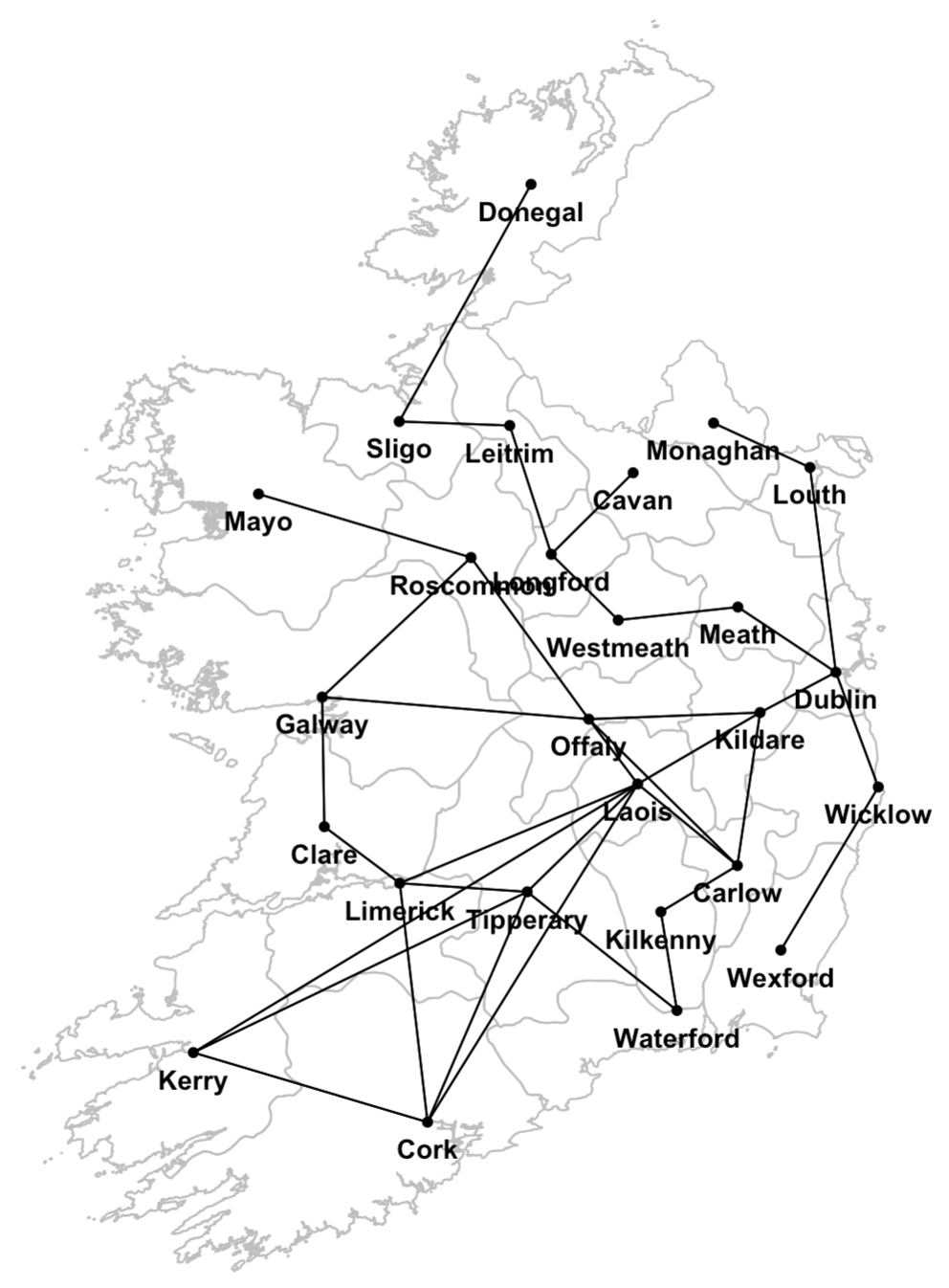
(a) Railway-based network

(b) Queen’s contiguity network

Figure 1: Map of Ireland and COVID-19 networks

3.2 Generalised network autoregressive models

Network-based Time Series models incorporate non-temporal dependencies in the form of networks in addition to temporal dependencies as established in time series models [1, 2, 34]. In contrast to standard time series methodology and spatial models [35, 36, 20], network-based time series models are not limited to geographic relationships but can incorporate any generic network. As COVID-19 is an infectious disease with spatial spreading behaviour, warranting constructing networks based on spatial information, we use terms relating to spatial dependence in our exposition. Other types of dependence could easily be incorporated in the model through networks which reflect the hypothesised dependence.

In this paper, we use the global $\alpha$ generalised network autoregressive models $GNAR(p,s)$ to model the observation $X_{i,t}$ for a vertex $i$ at time $t$ as the weighted linear combination of an autoregressive component of order $p$ and a network neighbourhood autoregressive component of a certain order (neighbourhood stage); for $i=1,\ldots,p$, the entry $s_{i}$ gives the largest neighbourhood stage considered for vertex $i$ when regressing on up to $p$ past values. The effect of neighbouring vertices depends on some weight $\omega_{i,q}$. Our GNAR model is given by

$$X_{i,t}=\sum_{j=1}^{p}\left(\alpha_{i,j}X_{i,t-j}+\sum_{r=1}^{s_{j}}\sum_{q\in N^{(r)}(i)}\beta_{j,r}\,\omega_{i,q}^{(t)}\,X_{q,t-j}\right)+\varepsilon_{i,t}$$ (1)

where $\varepsilon_{i,t}\sim N(0,\sigma^{2}_{i})$ are uncorrelated. This model is a special case of the GNAR model in [37, 38] . A typical choice for weighting is the normalised inverse shortest path length weight, where $d_{i,q}$ denotes the shortest path length (SPL) [2]; in connected networks, $1\leq d_{i,q}<\infty$ for $i\neq q$. For $i,q\in\mathcal{V}$ such that $q\in N^{(r)}(i)$,

$$\omega_{i,q}=\frac{d_{i,q}^{-1}}{\sum_{k\in N^{(r)}(i)}d_{i,k}^{-1}}\;.$$ (2)

The GNAR model (1) relies on vertex specific coefficients $\alpha_{i,j}$. The global-$\alpha$ model is a simplification of this GNAR model which assumes vertex unspecific autoregressive coefficients, $\forall i\in\{1,...,N\}:\;\alpha_{i,j}=\alpha_{j}$. We denote the GNAR model in (1) by GNAR$-p-s_{1},\ldots,s_{p}$-FALSE, to indicate vertex-specific coefficients $\alpha_{i,j}$; the global-$\alpha$ version is simply denoted by GNAR$-p-s_{1},\ldots,s_{p}$.

To fit a GNAR model, we must choose the lag $p$, or $\alpha$-order, and the vector of neighbourhood stages, $s=(s_{1},...,s_{p})$, also called $\beta$-order. They can be determined either through expert knowledge, e.g. on the spread of infections, or through a criterion-based search [2]. Consistent values for the GNAR coefficient are then estimated vy Least Squares (LS) estimation for i.i.d. error terms, or by Estimated Generalised Least Squares (EGLS) estimation for spatially correlated error terms [2, 38, 39].

3.3 GNAR model selection and predictive accuracy

For our analysis of the Irish COVID-19 data, model selection, i.e. the choice of $\alpha$- and $\beta$-order, is criterion-based. In accordance with [2], the model which achieves lowest Bayesian Information Criterion (BIC) is chosen. The BIC avoids overfitting by penalizing the likelihood for the data given a certain parametric distribution by the dimensionality of the required parameter [40]. For a sample $X$ of size $n$ and a parameter $\theta$ of dimension $k$,

$$\text{BIC}(k,n)=k\text{log}(n)-2\cdot\text{log}(L(X;\theta))\;.$$ (3)

The GNAR package assumes Gaussian errors [37]; under this assumption, the BIC is consistent. This assumption could be weaked; it can be shown that the BIC is consistent for the GNAR model (1) if the error term is i.i.d. with bounded fourth moments [38, 41, 42].

The predictive accuracy of a GNAR model is measured by the mean absolute scaled error (MASE). MASE is defined for each county $i$ as the ratio of absolute forecasting error $\hat{\varepsilon}_{i,t}=|X_{i,t}-\hat{X}_{i,t}|$ for some vertex $i$ divided by the mean absolute error between true and a naive 1-lag random walk forecast for the entire observed time period $[1,T]$ [43, 3].

$$|q_{i,t}|=\frac{|X_{i,t}-\hat{X}_{i,t}|}{\frac{1}{T-1}\sum_{l=2}^{T}|X_{i,l}-X_{i,l-1}|}\;.$$

MASE is chosen due to its insensitivity towards outliers, its scale invariance and its robustness [43].

4 Data Exploration

4.1 The weekly incidence differences

GNAR models require stationary data [2]. To remove any linear trend, we carry out 1-lag differencing of the weekly COVID-19 incidence for the 26 Irish counties, giving the incidence difference, (1-lag) COVID-19 ID, between two subsequent weeks [44]

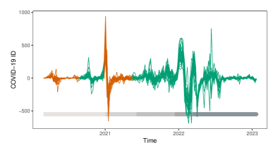
Figure 2: Weekly COVID-19 incidence difference (ID) for 100,000 inhabitants, from the start of the pandemic in March 2020 to mid June 2022, red for restricted phases, green for unrestricted; predominant COVID-19 virus variants shown by color scale at the bottom, in order: Original, Alpha, Delta, Omicron I and Omicron II

4.2 Constructed networks

First, we construct networks with the 26 counties as nodes. All but two of the network construction methods do not require any parameter settings; the exceptions are the KNN network and the DNN network. For the COVID-19 KNN network, neighbourhood sizes sequencing from $k=1$ to the fully connected network, $k=25$, by 2 steps are considered. The minimal distance for the COVID-19 DNN network measures 90.3 km, between Kerry and Cork, and the maximal value 338.5 km, between County Cork and Donegal. The KNN and DNN network parameters are chosen to minimise the BIC of the associated GNAR model. This is achieved for $k=21$ and $d=325$.

Table 1 shows average degree, average SPL and average local clustering coefficient for the 9 COVID-19 networks (excluding the complete network). There is considerable variability in particular regarding the network density, with the KNN and DNN networks having much larger average degree than the other networks; the sparsest network is the Relative neighbourhood network. Some of the ordering is not surprising; the Economic hub network expands the Queen’s contiguity network with additional edges between a county and its nearest economic hub. The degree for each vertex, and hence the average degree compared to the Queen’s contiguity network are increased by 1. Similarly, the SPL is shortest in the denser DNN and KNN networks. The Railway-based network has the longest average SPL due to its vertex chains and the low number of shortcuts between counties. For the Queen’s contiguity network, the introduction of shortcuts to the economic hubs leads to a decrease in average SPL, i.e. the disease spreads quicker. The Gabriel network is sparser than the SOI network, with slightly longer shortest path length. Deleting long edges in the Delaunay triangulation network to obtain the SOI network decreases the average degree and the average local clustering coefficient, but increases the average SPL. To assess small world behaviour, Table 1 also provides the corresponding average SPL and average local clustering for a Bernoulli $G(n,m)$ random graph on $n=26$ vertices, with the same number of edges as the constructed network. Small world behaviour would be indicated by an average SPL which is of the same order as the $G(n,m)$ graph, while having higher average local clustering coefficient. This criterion is satisfied for the Queen’s network, the Economic hub network, the Delaunay network, the Gabriel network, and the SOI network. The Railway network has much larger average SPL than the $G(n,m)$ network, while the dense KNN and DNN networks have almost the same average SPL and local clustering coefficient as the $G(n,m)$ network.

Metric	Railway	Queen	Eco. hub	KNN	DNN	Delaunay	Gabriel	SOI	Rel. neigh.
av. degree	5	4.38	5.38	23.54	24.85	5.15	3.69	4.15	2.31
av. SPL	4.15	2.74	2.27	1.06	1.01	2.41	3.02	2.86	3.99
av. local clust.	0.2	0.51	0.6	0.95	0.99	0.49	0.31	0.51	0
$G(n,m)$
av. SPL	1.99	2.25	1.99	1.06	1.01	2.04	2.43	2.42	4.16
av. local clust.	0.16	0.11	0.12	0.94	0.99	0.22	0.16	0.14	0

Table 1: Overview of network characteristics for the Railway-based, Queen’s contiguity, Economic (Eco.) hub, KNN ($k=21$), DNN ($d=325$), Delaunay triangulation, Gabriel, SOI, Relative neighbourhood (Rel. neigh.) network; including average (av.) degree, average (av.) shortest path length (SPL), average (av.) local clustering (clust.). The average shortest path length and average local clustering coefficient for a Bernoulli Random Graph $G(n,m)$, with $n=26$, for each network is also reported.

Real-world networks are frequently scale-free [45, 46], in the sense that the degree distribution possesses the scale-free property. As evident from calculations and log-log plots in the Supplementary Material A.2, no COVID-19 network fulfills this property.

4.3 Spatial effects

Next, we investigate whether the constructed networks capture any spatial correlation. Intuitively, for a spatial effect, the closer in SPL two vertices on a network are, the more highly correlated their COVID-19 incidences should be. We compute Moran’s I for each network, which measures spatial correlation across time [47, 48, 49]. For some time $t\in T$ and $x_{i}^{(t)}$ denoting the COVID-19 ID for county $i$ at time $t$, Moran’s I follows as the average weighted correlation across space,

$$I^{\,t}=\frac{\sum_{i=1}^{N}\sum_{j=1,i\neq j}^{N}w_{ij}\cdot(x^{(t)}_{i}-\bar{x}^{(t)})(x_{j}-\bar{x}^{(t)})}{W_{0}\cdot\frac{1}{N}\sum_{i}(x_{i}^{(t)}-\bar{x}^{(t)})^{2}}$$

where $W_{0}=\sum_{i,j=1}^{N}w_{ij}$ for normalisation. The weights $w_{ij}$ can be chosen arbitrarily. For the COVID-19 networks, we select inverse distance weighting where distance is measured in Great circle distance between the central points of two counties . This weighting is similar to that proposed in [51], suggesting exponential weights $w_{ij}=e^{-d_{ij}}$, to account for an exponential decrease in correlation as the SPL between vertices grows. The spatial dependency between counties varies strongly over time for every network, see Figure 3 and Figure 11 in Supplementary Material A.3. Peaks in Moran’s I coincide with peaks in the 1-lag COVID-19 ID at the beginning of the pandemic as well as during the winters 2020/21 and 2021/22. The introduction of restrictive regulations, e.g. lockdowns, lead to a decreasing trend in Moran’s I while the ease of restrictions from summer 2021 onward results in an increasing trend in Moran’s I. Hence, there is an indication of a network effect in the data, i.e. that the pandemic influence of one county on another is associated with the inter-county mobility of their inhabitants. This is in particular visible after the official end of restriction in March 2022.

For a statistical evaluation of the spatial dependency, we apply a permutation test in combination with Moran’s I to assess the relationship between network distance and COVID-19 case correlation. For each date, we permute the COVID-19 cases between counties $R=100$ times and compute Moran’s I with exponential weights [51]. A date-specific 95% credibility interval $\forall t=1,\dots,T:\;[m_{t,l},m_{t,u}]$ based on empirical quantiles ($q=0.025,0.5,0.975$ quantiles) is constructed. Under the null hypothesis, assuming no correlation between network structure and COVID-19 incidence, 5% ($0.05\cdot T\approx 8$) of observed Moran’s I values $m_{t}$ over time $t=1,\dots,T$ are expected to lie outside the time dependent 95% credibility interval, $[m_{t,l},m_{t,u}]$. If the proportion $N_{m}=T^{-1}\sum_{t}\{{\mathbb{I}(m_{t}>m_{t,u})+\mathbb{I}(m_{t}<m_{t,l})}\}$ of rejected tests over time is greater than expected under the null, we conclude that the network distance has an effect on the correlation between COVID-19 incidence.

The proportion of rejected tests is indicated for the restricted and unrestricted data set: Railway-based network $N_{m}=(0.25,0.142)$, Queen’s contiguity network $N_{m}=(0.227,0.217)$, Economic hub network $N_{m}=(0.25,0.179)$, KNN network $N_{m}=(0.091,0.151)$, DNN network $N_{m}=(0.068,0.094)$, Delaunay triangulation network $N_{m}=(0.205,0.189)$, Gabriel network $N_{m}=(0.114,0.132)$, SOI network $N_{m}=(0.182,0.198)$, Relative neighbourhood network $N_{m}=(0.159,0.189)$. The p-value for all network lies above the expected $\alpha=0.05$, supplying evidence for a relationship between network distances and case correlations. Depending on the network, the proportion for either the restricted or the unrestricted data set is larger.

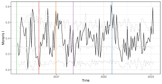
(a) Railway-based network

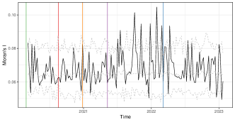
(b) KNN network (k = 21)

Figure 3: Moran’s I across time and global standardisation of shortest path-length (SPL) weights, main COVID-19 regulations by the Irish Government indicated by vertical lines; in order: initial lockdown, county-specific restrictions, Level-5 lockdown, allowance of inter-county travel, official end of all restrictions; 95% credibility interval in grey dashed

5 Results

5.1 GNAR model fitting

To assess whether GNAR models may be more appropriate than standard ARIMA models for the data, we compare standard ARIMA models with its their GNAR counterparts. The ARIMA models, fitted to each county individually, achieve a average $BIC=1846.882$ over all counties on the entire data set, $BIC=534.58$ for the restricted data set and $BIC=670.27$ for the unrestricted data set.

Optimal GNAR model for each COVID-19 network achieve much lower BIC. On the entire data set, the GNAR-5-11110 model with the KNN network ($k=21$) achieves the lowest $BIC=194.75$. For the restricted phase, the best GNAR models yield $BIC=91.41$ on the Queen’s contiguity network, and for the unrestricted phase $BIC=190.17$ on the KNN ($k=21$) network, see Table 2. This observation justifies the use of GNAR models here.

As detailed in Section 2, the nature of the virus suggests that the transmission of COVID-19 between Irish counties may depend strongly on the population flow between counties [52]. Protective COVID-19 restrictions taken by the Irish Government restricted and at times forbade inter-county travel in Level 3-5 lockdowns [53], [24]. As supported by the positive and negative trends in Moran’s I, the spatial dependence of COVID-19 incidence across counties is likely to have decreased during lockdowns and increased during periods in which inter-county travel was allowed [54]. This motivates training a GNAR model which is specific to pandemic phases.
Due to limited sample size, GNAR models cannot be fitted to each data subset defined by governmental COVID-19 restrictions. Therefore, we resort to concatenating datasets representing restricted and unrestricted pandemic phases.

5.2 Pandemic phases

Table 2 summarizes the optimal GNAR models and COVID-19 network for the restricted and unrestricted data set. For both phases, the best performing GNAR model select an autoregressive component of order 5.

The average residual as well as the average MASE are smaller for the restricted than the unrestricted pandemic phases, implying that here GNAR models are more suited to predicting periods with strict regulations than periods with fewer or no restrictions. The increase in accuracy here is associated with higher variance. The optimal network for the unrestricted pandemic phase is much denser than the optimal network for the restricted phase. This might indicate the effect of inter-county travel bans on COVID-19 infections. As evident from Tables 4, 5 in Supplementary Material D.1, the BIC value for the optimal GNAR model lie within the range $[91.41,93.27]$ for the restricted data set and within the range $[190.17,192.54]$ for the unrestricted data set. Figure 13 in Supplementary Material D.1 illustrates that denser networks perform better for the unrestricted data set while sparse networks achieve lower BIC for the restricted data set.

Data subset	network	GNAR model	BIC	$\bar{\varepsilon}$ (sd)	av. MASE (sd)
Restricted	Queen	GNAR-5-21111-TRUE	91.41	0.19 (17.06)	0.91 (0.76)
Unrestricted	KNN-21	GNAR-5-11110-TRUE	190.17	-13.08 (14.6)	0.93 (0.72)
Restricted	ARIMA		534.58	-0.78 (19.08)	1.22 (1.34)
Unrestricted	ARIMA		670.27	-16.65 (18.5)	1.21 (0.97)

Table 2: Overview over the best performing model and network for restricted and unrestricted pandemic phases; average residual $\bar{\varepsilon}$ and average (av.) MASE indicated for the predicted 5 weeks at the end of the observed time period across all counties, 11.04.2021 - 09.05.2021 for the restricted dataset and 25.12.2022 - 23.01.2023 for the unrestricted dataset; standard deviation (sd) across counties in brackets.

A decrease in inter-county dependence due to COVID-19 restrictions should result in decreasing values for the $\beta$-coefficients in the GNAR model. This hypothesis can only be partially verified, see Figure 4. The absolute value of $\beta$-coefficients increases from the restricted to the unrestricted phase, implying increased spatial dependence after COVID-19 restrictions have been eased or lifted. Interestingly, the GNAR model picks up a decrease in temporal dependence in COVID-19 ID. As a disease spreads more freely due to lenient or no restrictions, it has been observed in other data studies that case numbers can grow more erratic and become less dependent on historic data [55], [6]. This effect, in addition to peaks and high volatility in COVID-19 ID observed during pandemic phases with less restrictive regulations, might contributed to the negative $\alpha$-coefficient values for the unrestricted data set.

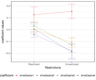
(a) $\alpha$-order

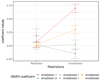
(b) $\beta$-order

Figure 4: Development of GNAR model coefficients for the restricted and unrestricted pandemic phase; restricted phase with Queen’s contiguity network, unrestricted phase with KNN network

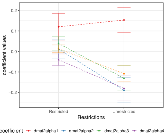
(a) $\alpha$-order

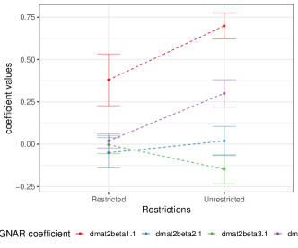
(b) $\beta$-order

Figure 14: Development of GNAR model coefficients for the restricted and unrestricted pandemic phase for the optimal GNAR model $GNAR(\alpha=5,\beta=(1,1,1,1,0))$ for the KNN network with $k=21$

Identical observations can be made when considering how the coefficients develop between the restricted and unrestricted phase for the GNAR model that is optimal for the entire data set, namely, $GNAR(\alpha=5,\beta=(1,1,1,1,0))$ with the KNN ($k=21$) network; the $\beta$-coefficients increase in absolute value for the unrestricted phase compared to the restricted phase, see Figure 14 in Supplementary Material D.2.

The predictive accuracy for both datasets is comparable and varies from county to county, see Figures 5 and 6 for 9 example counties, MASE values for the remaining counties follow similar patterns. For the restricted phase, GNAR models achieve lower MASE than the ARIMA models except for counties Donegal, Cavan, Leitrim, Monaghan and Sligo, for which the ARIMA model performs equally well. These counties border to Northern Ireland and might suffer from a border effect between the Republic of Ireland and Northern Ireland. Throughout the pandemic, no strict border closure between Ireland and Northern Ireland was enforced [56], [57]. The constructed GNAR models based on Ireland-restricted networks do not account for the disease spread across the Irish border.

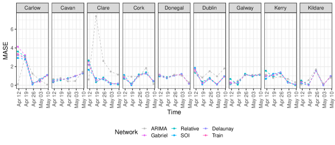
(a) Delaunay triangulation, Gabriel, Relative neighbourhood, SOI and Railway-based network

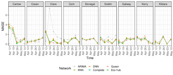
(b) KNN $k=7$, DNN $d=200$, Complete, Queen’s contiguity and Economic hub network

Figure 5: MASE values for the restricted pandemic phase, for 9 selected counties

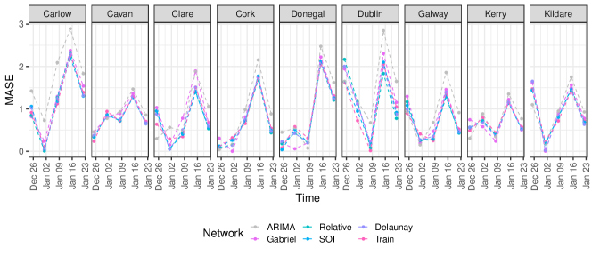
(a) Delaunay triangulation, Gabriel, Relative neighbourhood, SOI and Railway-based network

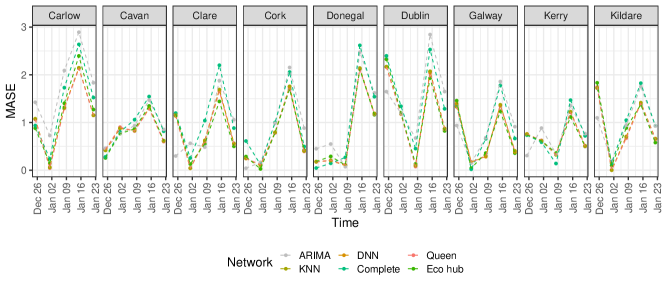
(b) KNN $k=21$, DNN $d=325$, Complete, Queen’s contiguity and Economic hub network

Figure 6: MASE values for the unrestricted pandemic phase, for 9 selected counties

For the restricted phase, the predictions differ more strongly between the GNAR model and the ARIMA model, see Figure 16 in Supplementary Material D.3. For the unrestricted phase, the GNAR and ARIMA models follow roughly the same trajectory while achieving smaller residuals for most counties. This might imply a stronger network effect during the unrestricted pandemic phase and may point to some efficiency of COVID-19 regulations to contain inter-country spread.

The above model fits assume that the observations follow a Gaussian i.i.d. error structure. To assess this assumption, we test whether the residuals $\hat{\varepsilon}_{i,t}$ follow a normal distribution with a county-specific Kolmogorov-Smirnov test, aggregated over time. We obtain primarily insignificant p-values across counties for the restricted phase ($\#p\leq 0.025=6$, $\#p>0.025=20$) and majority significant p-values across counties for the unrestricted phase ($\#p\leq 0.025=21$, $\#p>0.025=5$). Table 6 in Supplementary Material D.4 details the average MASE, average residual and p-value for each county, resulting for the two optimal GNAR models for the restricted and unrestricted data set. The Gaussian nature of residuals indicate suitability of the GNAR model to model restricted pandemic phases and ensure consistency in coefficient estimates. For the unrestricted phase, the Gaussianity in the model assumptions could not be statistically verified. These conclusions are supported by the county-specific QQ-plots in Supplementary Material D.4 .

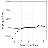
(a) Restricted

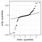
(b) Unrestricted

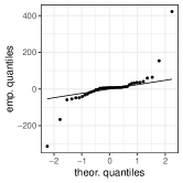
(c) Restricted

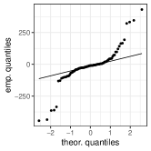
(d) Unrestricted

Figure 7: QQ-plot for the residuals from the best performing GNAR model and network for restricted and unrestricted pandemic phase for county Dublin (left) and Donegal (right)

The GNAR model further assumes that the errors are uncorrelated. To assess this assumption, the residuals are investigated according to their temporal as well as spatial autocorrelation by applying the Ljung-Box test and Moran’s I based permutation test [58], [48]. The former concludes significant temporal correlation for short-term lags in the GNAR residuals for each county. Thus there is evidence that the GNAR model insufficiently accounts for temporal dependence in COVID-19 incidence in subsequent weeks. The residuals show remaining spatial autocorrelation. The Moran’s I based permutation test counts $N_{m}=9$ Moran’s I values outside the corresponding 95% credibility interval (expected $0.05\cdot 45\approx 2$) for the restricted phase and $N_{m}=16$ for the unrestricted phase (expected $0.05\cdots 107\approx 5$). The reduction in spatial correlation for the restricted phases and the Queen’s contiguity is greater ($N_{m}=10$ on COVID-19 cases to $N_{m}=9$ for residuals) than for the unrestricted phases and the KNN network ($N_{m}=16$ for COVID-19 cases and residuals). We conclude that there is evidence that the GNAR model insufficiently incorporates the spatial relationship in COVID-19 case numbers across counties. These possible violations of the model assumptions have to be taken into account when interpreting the model fit.

6 Discussion

In this paper, we modelled the COVID-19 incidence across the 26 counties in the Republic of Ireland by fitting GNAR models, leveraging different networks to represent spatial dependence between the counties. We found that the GNAR model performs better on data collected during pandemic phases with inter-county movement restrictions than data gathered during less restricted phases. Sparse networks perform better for the restricted data set, while denser networks achieve lower BIC for the unrestricted data set, implying higher spatial correlation in COVID-19 incidence during pandemic periods with fewer restrictions. In addition, the GNAR model coefficient values hint at the efficiency of movement regulations. Here we discuss these findings in more detail, including limitations and challenges.

A key challenge for modelling is that COVID data is characterised by high uncertainty e.g due to testing hesitancy, low testing capacity and double counting [59, 18, 60]. In general, such uncertainty is typical for data of spreads of epidemics [54]. For COVID-19 in particular, incidence data is extremely erratic due to its tendency for fast and sudden local outbreaks and due to many unreported cases [61, 23].

6.1 Choice of network

The fitted GNAR models make use of different underlying networks. While the performance of COVID-19 networks are similar, as ellaborated on in Section 5.2, each network has different assumptions and implications. The DNN network requires its lowest upper bound to be chosen such that it is larger than the maximum distance between any vertex and its nearest neighbour. The number of edges increases rapidly as the upper boundary increases. Hence, if the distance to the nearest neighbours varies greatly between vertices, i.e. the data is irregularly spaced, this requirement will result in high degree heterogeneity between the vertices [33]. The KNN network per construction connects each county with its $k$ nearest neighbours, obtaining a homogeneous degree distribution with little variability around the average degree $k$. Consequently, the KNN network cannot account for heterogeneity in connectivity between counties, e.g. due to areas with higher population exchange or higher COVID-19 transmission rate. The Complete network assumes homogeneous mixing between the counties [33]. The validity of such assumption for pandemic phases with movement restrictions can be questioned while it can be considered suitable for phases with free movement.

Despite the low popularity of train traveling in Ireland, even the railway-based network seems to capture relevant population flow between counties informing the spread of COVID-19. The Delaunay triangulation networks as well as its induced networks, the Gabriel, Relative neighbourhood and SOI network, suffer from low interpretability, given their general geometrical approach to constructing neighbourhoods. The construction approach bases on a certain geometrical understanding of proximity between vertices which can be criticised as arbitrary because it is not contextually validated [29, 31, 32, 67, 68] . For disease modelling, networks ideally mirror the reality of disease transmission through population flow [3]. The Queen’s contiguity network connects all geographically neighbouring counties. The Economic hub model strives to capture additional human movement, e.g. commuting, by expanding the Queen’s contiguity networks with edges to the nearest economic hub.

6.2 Choice between ARIMA and GNAR

In general, ARIMA models are considered useful for short term predictions of the spread of epidemics [54]. Here we find that GNAR models outperform ARIMA models for both pandemic phases. The ARIMA models are fitted to each county individually, requiring a large number of parameters compared to global-$\alpha$ GNAR models. In a trade-off between predictive accuracy and number of parameters we would tend to prefer the constructed global-$\alpha$ GNAR models over ARIMA models. High dimensionality in model coefficients can result in high instability in the form of large standard deviation [69]. In GNAR models, the model parametrisation relies on the underlying networks. This guarantees parsimonious models and provides a model inherent dimensionality reduction [69].

In general, GNAR models seem more suited to modeling COVID-19 incidence if inter-county movement is restricted. The residuals for the restricted phases can be considered Gaussian. According to the performed Kolmogorov-Smirnov tests, the residuals for the unrestricted phases as well as for the GNAR model fit to the entire COVID-19 data disregarding the different phases deviate from the Gaussian distribution. The parameter estimates for the GNAR model require independent error terms with a bounded fourth moment to be consistent and asymptotically normal. These requirements are obviously fulfilled by Gaussian white noise. If the error term is not Gaussian and does not fulfill the conditions, alternative, computationally more intensive approaches, such as the Newton-Raphson method [70] or the Iteratively Reweighted Least Squares method [71], should be implemented, in particular to correctly draw inference.

In light of the discrete nature of the COVID-19 case counts and the challenge of structural misreporting, alternative error structures, e.g. according to a Poisson process, are plausible [72]. To the best of our knowledge, methods to estimate model coefficients while assuming such error structures in the context of GNAR models have not yet been developed.

6.3 Interpreting the model fit

The fitted GNAR models have different coefficients for the restricted and for the unrestricted phase. The effect of COVID-19 restrictions is not systematically detectable in the $\beta$-order, e.g. restricting inter-county travel leading to lower stage neighbourhoods or even $\beta=0$. However, the change of restrictions is reflected in the change in values of the $\alpha$- and $\beta$-order coefficients in the subset-specific models. Nevertheless, GNAR models seem unsuited to quantify the effectiveness of COVID-19 regulations to the same extent as alternative COVID-19 models do which are more tailored to address this effectiveness, e.g. [59, 73, 74].

The best performing GNAR models are more complex, i.e. have larger $\alpha$- and $\beta$-order, than the GNAR models commonly implemented, e.g. in [1, 2, 3]. It is possible that the higher orders hint at stronger temporal and spatial dependence. The fitted GNAR models benefit from leveraging values further back in history as well as the historic values of neighbours. The spatial dependence decreases over time, leading to smaller stage neighbourhoods for larger lags.

For model selection, the BIC and MASE do not agree in their consequences, in particular regarding the comparison between GNAR and ARIMA model. This observation emphasises the importance of choosing a criterion for model selection which corresponds to the desired task. To predict the COVID-19 incidence, the MASE contains more information to assess model accuracy. The BIC value weighs the likelihood of the data given a certain parametrisation of the GNAR model against the number of parameters fitted in the model. The BIC computation in the GNAR package assumes the error term, and hence $X_{t}$, to be Gaussian [37]. As detailed in Section 5.2, we could not validate this assumption for the unrestricted phase and the deviation from the assumption might explain the poor performance of the BIC in identifying models with high predictive accuracy.

To disentangle the performance of the model from violated model assumptions, we carried out a simulation study, in which data was generated on a well defined network with Gaussian error with mean zero and unit variance, using GNAR-5-2111 model on the Queen’s contiguity network and SPL weighting.

To further assess the stability of the results, in Supplementary Material E data are simulated from the best-fitting GNAR model for the restricted data set. However we found that the GNAR model could not accurately reconstruct the coefficients, see Tables 7 and 8 in Supplementary Material E. This finding points to the need to further investigate possible limitations of GNAR models.

7 Conclusion

In general, a network model could can be a powerful tool to inform the spread of infectious diseases, see for example [75, 76]. This paper analyses how accurately GNAR models relying on differently constructed networks predict COVID-19 cases across Irish counties. While we do not assume that the disease only spreads along the network, we consider the edges to represent the main trajectory of the infection. The analysis shows that no network is consistently superior in predictive accuracy. GNAR models seem relatively robust to the exact architecture of the network, as long as it lies within a certain density range. Our analysis suggest that unrestricted pandemic phases require dense networks, while restricted pandemic phases are better modelled by sparse networks.

For our data, the GNAR model is better suited to model the pandemic phases with strict movement regulations compared to those with more lenient or no restrictions. There are some caveats relating to the model. First, COVID-19 is also subject to “seasonal” effects, e.g. systematic reporting delays due to weekends and winter waves [16, 77, 17]. The GNAR model does not have a seasonal analogue which can incorporate seasonality in data, like SARIMA for ARIMA models [78]. Future work might introduce a seasonal component to the GNAR model, improving its applicability to infectious disease modelling.

Moreover, the COVID-19 pandemic had a strong influence on mobility patterns [66, 79], in particular due to restrictions of movement and an increased apprehension towards larger crowds. Considering only static networks may introduce a bias to the model [33, 8, 80]. Future work could therefore explore how GNAR models can include dynamic networks to incorporate a temporal component of spatial dependency.

Regarding the theory of GNAR models, alternative error distributions, in particular a Poisson distributed error term, could be explored given the indication of non-Gaussian residuals for the unrestricted pandemic phase. Alternative weighting schemes for GNAR models could be investigated to account for differences in edge relevance across time and network. The stability of parameter estimation in GNAR models also warrants further investigation.

The network constructions themselves could also be refined. Future analysis could focus on more content-based approaches to constructing networks, e.g. building a network based on the intensity of inter-county trade, computed according to the gravity equation theory [81]. To our knowledge, neither GDP nor trade data is reported in Ireland on a county level. Many researchers have successfully modelled the initial spread of COVID-19 from Wuhan across China based on detailed mobility patterns, e.g. [5, 6]. Such models require more detailed information on population flow and the origin of COVID-19 infections (e.g. local infection, domestic or international travelling). Partly due to data protection and privacy rights, comparable data of human movement on a level as granular as the Chinese is not publicly available [82, 83]. The performance of network based statistical models is hence also determined by the availability - or unavailability - of sufficiently detailed data [84]. Finally, in our statistical analysis the information about the dominant strain was not included. With COVID-19 being an evolving disease, it is possible that different strains may display different transmission patterns. If more detailed data become available then this question would also be of interest for further investigation.

Acknowledgements.

G.R. acknowledges support from EPSRC grants EP/T018445/1, EP/X002195/1, EP/W037211/1, EP/V056883/1, and EP/R018472/1.

Supplementary Material

Appendix A COVID-19 networks

A.1 The constructed networks

The COVID-19 networks are constructed according to either a geographical understanding or a statistical approach to neighbourhood. Figure 1 in the main text shows the Railway-based network and the Queen’s continguity network. Here we show the remaining networks, with parameter $k=21$ for the KNN network, and $d=325$ for the DNN. Figures 9 and 8 show the constructed COVID-19 networks, grouped by the geographical definition of neighbourhoods using the Great Circle distance, and by the geometric definition of neighbourhoods based on triangulations.

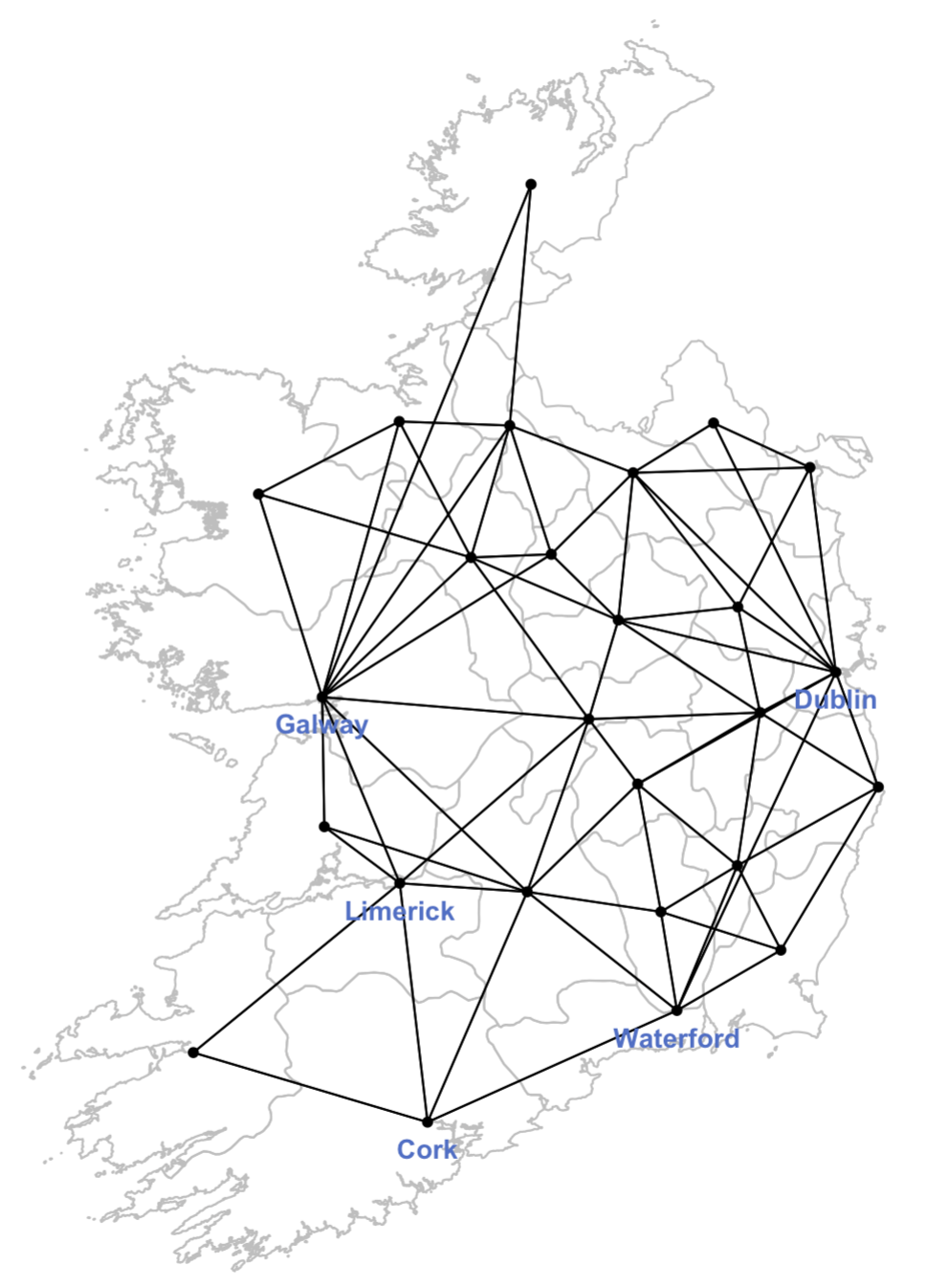
(a) Economic hub network

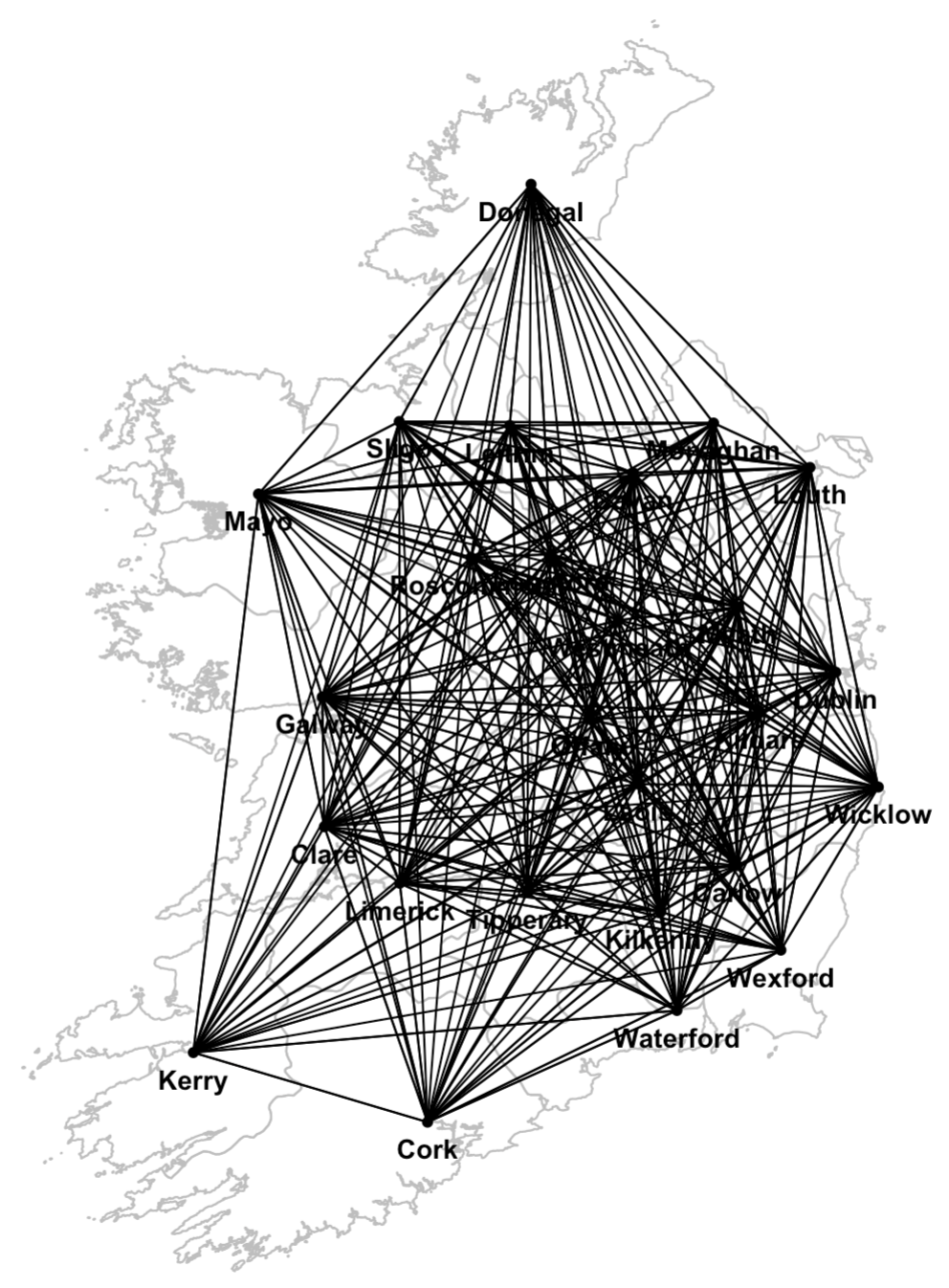
(b) KNN network (k = 21)

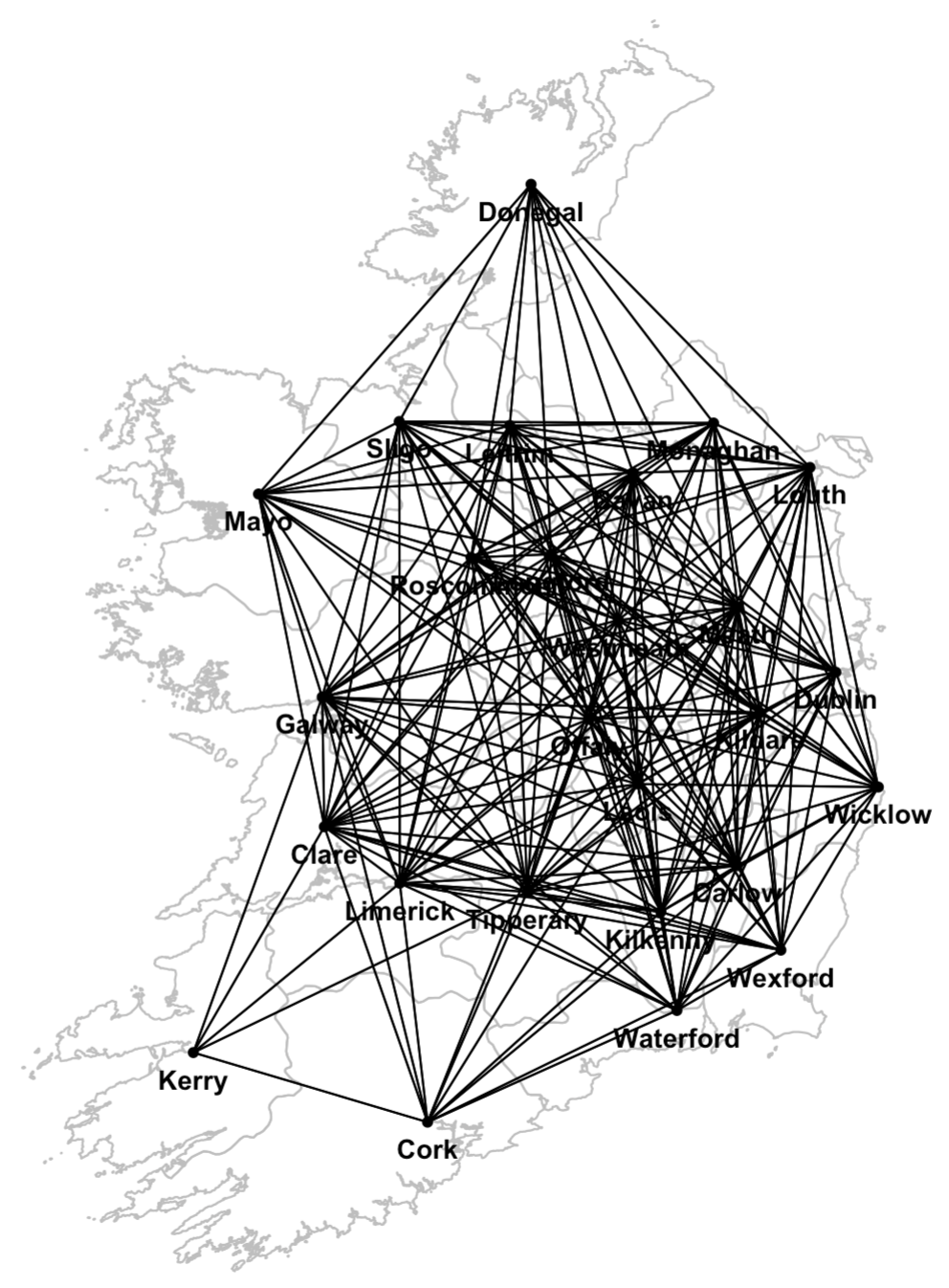
(c) DNN network (d = 325)

Figure 8: Map of Ireland and COVID-19 networks - based on Great Circle distance; economic hub towns marked in blue for Figure (a)

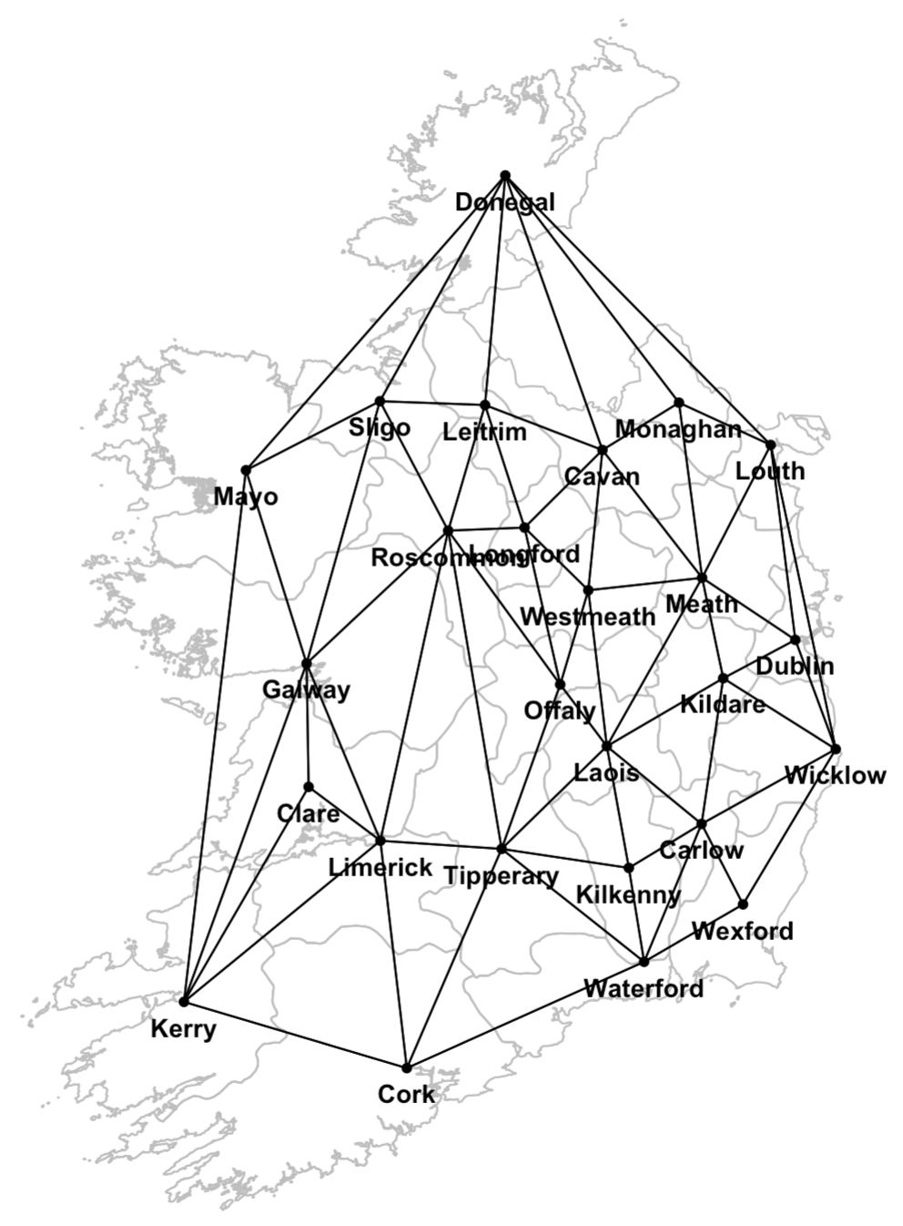
(a) Delaunay triangulation network

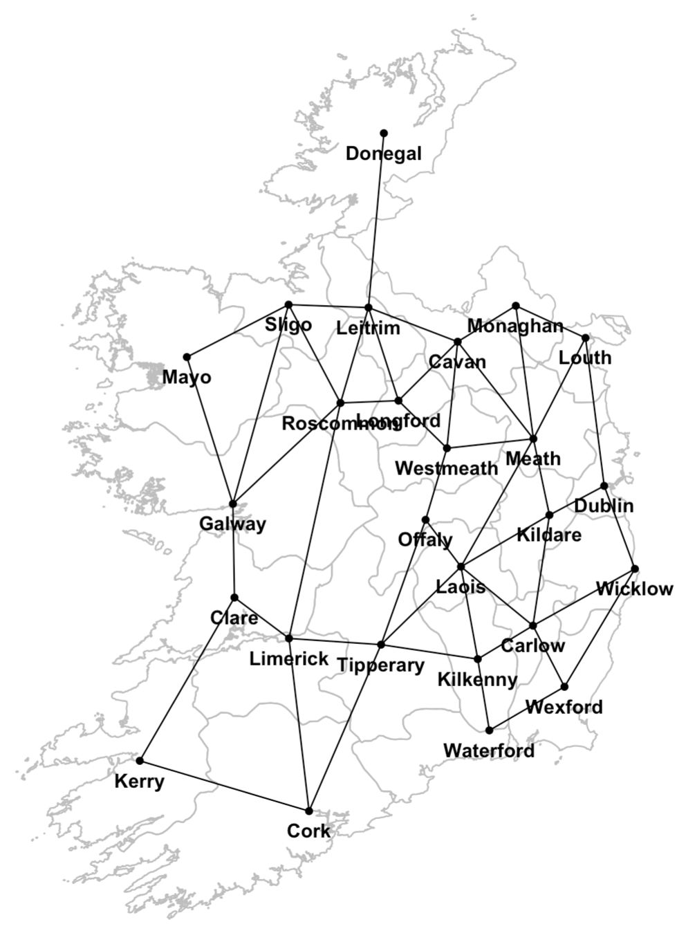
(b) Gabriel network

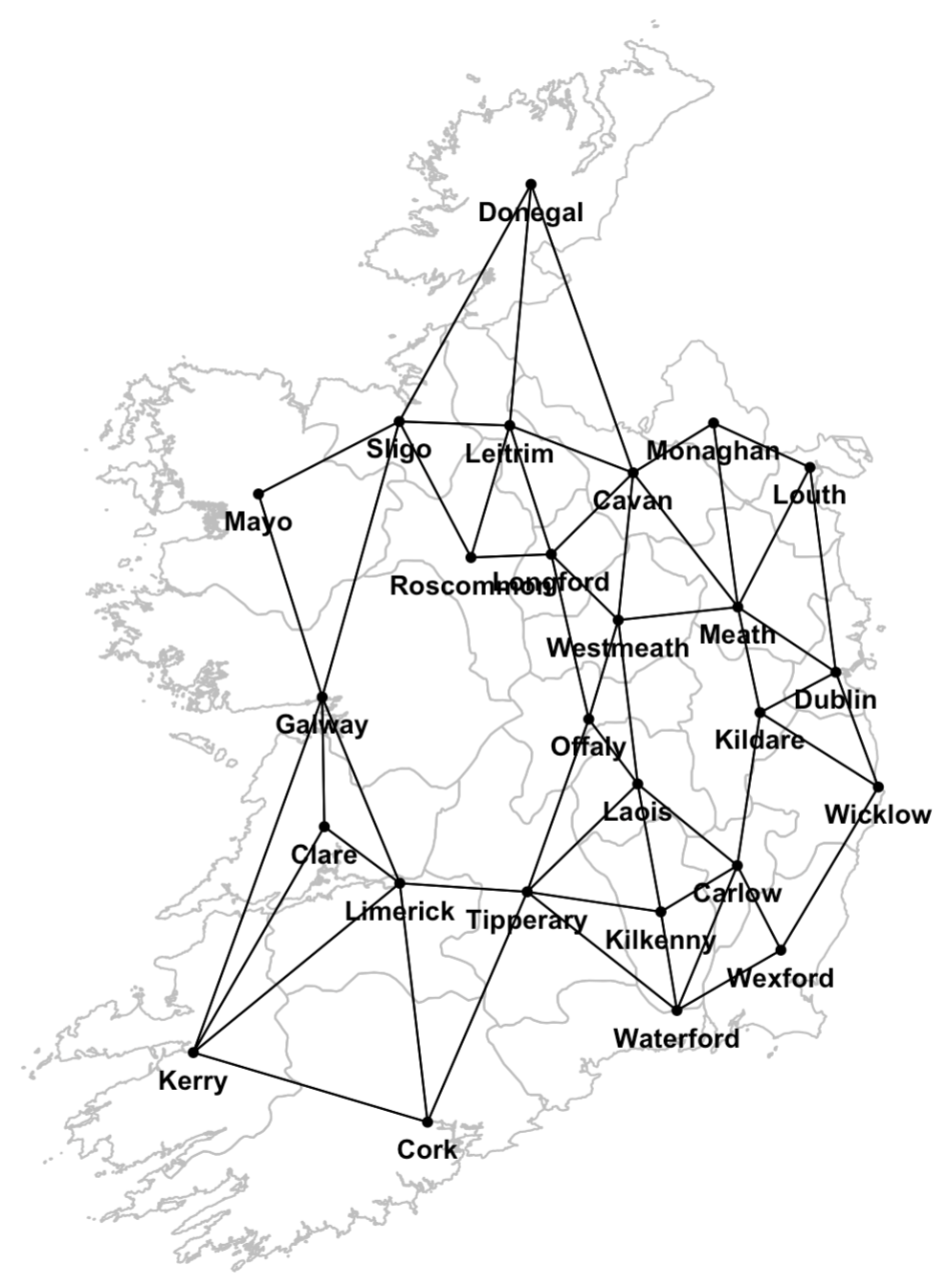
(c) SOI network

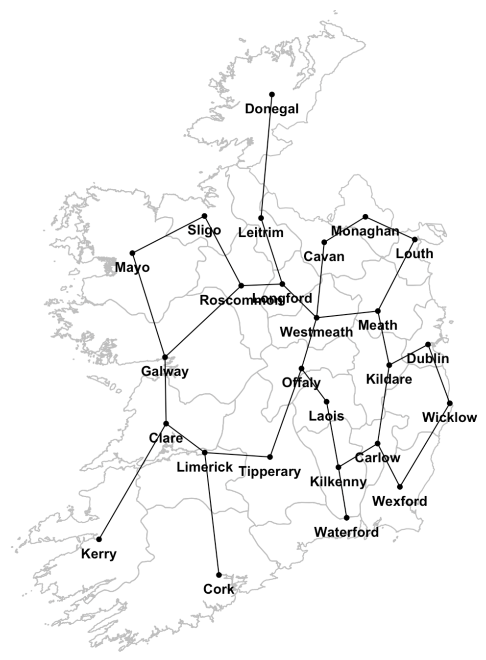
(d) Relative neighbourhood network

Figure 9: Map of Ireland and COVID-19 networks - based on geometrical definition of neighbourhoods

A.2 Assessing the scale-free property for fitted COVID-19 networks

The scale-free property of the COVID-19 networks is determined by the adjusted log-log plot after [46] which should cover at least three orders of magnitude to be considered adequate proof [85]. This is not the case for the Economic hub, the Delaunay triangulation, the SOI, the KNN and the DNN network. All remaining networks show a non-linear plot and hence scale-dependent behaviour, see Figure 10. This conclusion is corroborated by the $R^{2}$ values from a least-squares fit to the log-log plot. For a scale-free networks, the value for $R^{2}$ should lie above 0.99[46, 85]; none of our networks satisfy this criterion.

Network	$R^{2}$
Railway-based	0.96
Queen	0.97
Economic hub	0.95
KNN	0.98
DNN	0.96
Delaunay triangulation	0.94
Gabriel	0.98
SOI	0.90
Relative neighbourhood	0.94

Table 3: Test for scale-free property for each network: $R^{2}$ follows from the regression of the log empirical cumulative distribution on the log transformed degree $d$.

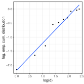
(a) Railway-based network

(b) Queen’s contiguity network

(c) Gabriel network

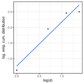
(d) Relative neighbourhood network

Figure 10: Scatter plot of the log transformed degree (d) against the log transformed empirical cumulative distribution for the networks for which the degrees span at least three orders of magnitude

A.3 Assessing the network effect via Moran’s I

Figure 3 in the main text shows Moran’s I across time for the KNN network and the Railway-based network. Here in Figure 11, we provide the results for the other networks. For the Delaunay triangulation, Gabriel, SOI and Relative neighbourhood network, Moran’s I follows a similar pattern, due to the induced nature of the networks. The Queen’s and Economic hub network show different trajectories in Moran’s I despite their similarity.

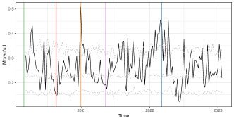
(a) Queen’s network

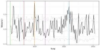
(b) Economic hub network

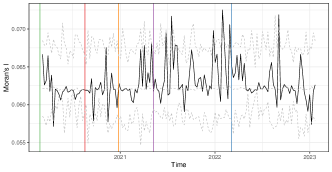
(c) DNN network ($d=325$)

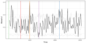
(d) Delaunay triangulation network

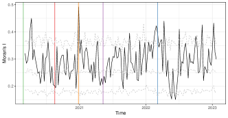
(e) Gabriel network

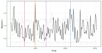
(f) SOI network

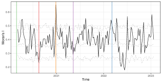
(g) Relative neighbourhood network

Figure 11: Moran’s I across time and global standardisation of SPL weights, main COVID-19 regulations by the Irish Government indicated by vertical lines; in order: initial lockdown, county-specific restrictions, Level-5 lockdown, allowance of inter-county travel, official end of all restrictions; 95% credibility interval in grey dashed

Appendix B GNAR models

B.1 Further background on network-based time series models

Network time series models expand multivariate time series by incorporating non-temporal dependencies. Such dependencies are represented by a network. An edge indicates a certain relationship between the variables which are represented by the two vertices. The output variable at each vertex is modelled to depend on its own past values as well as the past values of its neighbouring vertices which are determined by the network underlying the model. A myriad of methods for multivariate time series analysis exist [36].

Spatial Autoregressive and Moving Average models

The development of network time series models has drawn inspiration from models for spatial observations. [86] developed the spatial autoregressive model (SAR) which models the value at a certain vertex as a weighted average across a vertex-specific re-defined location set and an additive random error. Such model can be expanded to a mixed regressive-autoregressive model by incorporating exogenous variables $Y$. [87] utilises this model to account for "the geography of social phenomena" ([87], p. 359-360). [86] also introduces an alternative model relying on autoregression in the error term. [88] extends these models to spatial network autoregressive models (SARMA) that include a weight matrix $W$ which encodes the spatial dependencies; see [89] for choices of $W$.These models have been explored in numerous papers (e.g. [90, 91, 92, 93, 94, 95]). However, all above mentioned models do not take any time dependence into account, see [38], and require Gaussian error term with homoscedastic variance.

Temporal extensions

The m-STAR model by [96] models a spatial as well as a temporal dependence, restricted to 1-lag autoregression. The sets of spatial weights represent network interdependence between vertices on different contextual levels. The spatial temporal conditional autoregressive model (STCAR) is a continuous Markov random field with a Gaussian conditional probability density function. Its distributions rely on a space-time autoregressive matrix which accounts for both spatial and temporal dependencies. A very general model choice is the vector autoregression model (VAR). A VAR model regresses a vector at time on its values at previous time points, according to its order which is restricted by the size of the data set [97, 38]. While general VAR models can model data which are represented by networks, they would typically include one parameter per edge in the network and are hence often too large to be of practical use. Hence specifications to network data have recently been developed, as follows.

Network autoregressive models

For network time series, [34] established a particular VAR model, the network autoregression model. It includes an intercept and exogenous variables while time dependence is restricted to lag 1. Network autoregression follows the tradition of SMA and SAR models but incorporates historic values of the vertex in question and its $1^{st}$-stage neighbourhood. To ensure less sensitivity to outliers in the data and to incorporate heteroscedasticity, the paper [98] expanded the model to network quantile autoregression [98]. The paper [99] further develops the grouped network autoregressive model (groupNAR) which breaks the homogeneity by attributing each vertex to a group and estimating group-specific coefficients. The classification of the vertices is learned simultaneously with the parameter estimation. The number of classes has to be pre-specified [99].

Similarly to the 1-stage network autoregressive model, the network autoregression model NAR(p,s) includes historic values of the observation itself as well as its neighbours while assuming stationarity and spatial network homogeneity, with a general choice of lags and of neighbourhood stages.

The network autoregressive (integrated) moving average models (NARIMA) resemble restricted vector autoregressive (VAR) models with restriction reflecting the underlying network, [1, 2]. NARIMA models facilitate dimensionality reduction and allow great flexibility in modelling spatial and temporal dependencies [1, 38]. A NARIMA model consists of a NAR component, $X_{t}$, and a moving average component of order q (MA(q)), $\sum_{l=1}^{q}\eta_{l}\varepsilon_{i,t-l}$

$$X_{i,t}=\sum_{j=1}^{p}\left(\alpha_{j}X_{i,t-j}+\sum_{r=1}^{s_{j}}\sum_{q\in N^{(r)}(i)}\beta_{j,r}X_{q,t-j}\right)+\sum_{l=1}^{q}\eta_{l}\varepsilon_{i,t-l}+\varepsilon_{i,t}\;.$$ (4)

The relevance of vertices is acknowledged by vertex-specific weights [2]. The choice of weights strongly depends on the scenario and content the model is applied to [89].

$$X_{i,t}=\sum_{j=1}^{p}\left(\alpha_{j}X_{i,t-j}+\sum_{r=1}^{s_{j}}\sum_{q\in N^{(r)}(i)}\beta_{j,r}\omega_{i,q}X_{q,t-j}\right)+\sum_{l=1}^{q}\eta_{l}\varepsilon_{i,t-l}+\varepsilon_{i,t}\;.$$ (5)

The gNARIMA model generalises (4) by incorporating time dependent weights $\omega_{i,q,t}$ which allow excluding some of the vertices some of the time [2]. All above models do not incorporate any exogenous variables and can only integrate one network [2, 38]. The GNAR model (1) used in this paper is an adaptation of the gNARIMA model 5 with autoregressive weights $\alpha_{i,j}$ which are allowed to depend on the vertex itself, but without a moving average component.

B.2 The GNAR model in matrix form, and generalised least squares estimation

We can rewrite the GNAR model (1) in matrix form

$$X=BZ+\varepsilon$$

with $X=[X_{p+1},...,X_{T}]$ and $Z=[Z_{p},...,Z_{T-1}]$ where $Z_{t}^{T}=[X_{t},...,X_{t-p+1}]$. The matrix $B=[\phi_{1},...,\phi_{p}]$ summarises $\alpha$- and $\beta$-coefficients in the form $\phi_{j}=\text{diag}(\alpha_{\alpha_{i,j}})+\sum_{r=1}^{s_{j}}\beta_{j,r}\,W^{(r)}$, where $W^{(r)}$ denotes the weight matrix with $[W^{(r,}]_{l,m}=\omega_{l,m}\cdot\mathbb{I}_{m\in N^{(r)}(l)}$. The random error matrix is expressed by $\varepsilon=[\varepsilon_{p+1},...,\varepsilon_{T}]$, where the vector $\varepsilon_{t}=(\varepsilon_{1},...,\varepsilon_{n})\sim(0,\Sigma_{\varepsilon})$ is iid. with variance $\Sigma_{\varepsilon}=\sigma^{2}\cdot I_{N\times N}$ [1].

GNAR implies restrictions $R\in\mathbb{R}^{pN^{2}\times M}$ on the parametrisation,

$$vec(B)=\phi=R\gamma$$ (6)

where $vec(B)$ describes the reformatting of matrix $B$ into a vector by stacking its columns, the vector $\phi$ denotes the unrestricted coefficient vector for a VAR model and the vector $\gamma$ consists of the $M$ unrestricted parameters. For a vertex-specific GNAR model, $M=Np+\sum_{j=1}^{p}s_{j}$ and for a global-$\alpha$ model, $M=p+\sum_{j=1}^{p}s_{j}$ [1]. The Least Squares (LS) estimation finds $\hat{\phi}$ such that it minimises the sum of squares [39],

$$\hat{\phi}=\text{argmin}_{\phi}\,tr\left((X-BZ)^{T}\Sigma_{\varepsilon}^{-1}(X-BZ)\right)=\left((ZZ^{T})^{-1}Z\otimes I_{N}\right)\cdot vec(X),$$

where $\otimes$ denotes the Kronecker product. For the re-parametrisation imposing constraints in (6), the Generalised Least Squares estimation (GLS) computes

$$\hat{\gamma}=\left(R^{T}(ZZ^{T}\otimes{\Sigma}_{\varepsilon}^{-1})R\right)^{-1}R(Z\otimes{\Sigma}_{\varepsilon}^{-1})\cdot vec(X)$$ (7)

[1, 100]. The GLS estimator is consistent and asymptotically follows a normal distribution if $\{X_{t}\}_{t}$ is stationary and $\varepsilon_{t}$ a standard white noise process. It is identical to the Maximum Likelihood estimator if we assume $\varepsilon_{t}$ to be Gaussian [39]. However, the GLS estimator requires knowledge of the error covariance matrix $\Sigma_{\varepsilon}$ which is usually unknown. The Estimated GLS estimator (EGLS) substitutes the true covariance matrix in the estimation (7) with a consistent estimator $\hat{\Sigma}_{\varepsilon}$ which converges to $\Sigma_{\varepsilon}$ in probability as $n\to\infty$ [39],

$$\tilde{\gamma}=\left(R^{T}(ZZ^{T}\otimes\hat{\Sigma}_{\varepsilon}^{-1})R\right)^{-1}R(Z\otimes\hat{\Sigma}_{\varepsilon}^{-1})vec(X)\;.$$ (8)

The matrix $R^{T}(ZZ^{T}\otimes\hat{\Sigma}_{\varepsilon}^{-1})R$ must be non-singular which holds with probability 1 for continuous $X_{t}$ [39]. The estimate $\tilde{\gamma}$ is consistent and asymptotically normal if $\varepsilon$ is standard white noise. For a stationary time series with standard white noise, the EGLS estimate (7) and GLS estimate (7) are asymptotically equivalent [39]. Under stationarity and standard white noise error, a possible choice for a consistent estimator $\hat{\Sigma}_{\varepsilon}$ is

$$\hat{\Sigma}_{\varepsilon}=\frac{1}{T}(X-\hat{B}Z)(X-\hat{B}Z)^{T}$$ (9)

where $\hat{B}$ follows from the unconstrained LS estimate (B.2) and a corresponding transformation to obtain matrix $\hat{B}$ [39]. We obtain $\tilde{B}$ by inserting the EGLS estimate for $\gamma$ into (6) [1],

$$\widehat{vec(B)}=R\tilde{\gamma}\;.$$

B.3 Choices for the order of the model

We iterate through all possible combinations of $\alpha$-order $p\in\{1,...,5\}$ and $\beta$-order: [0], [1], [1, 0], [1, 1], [2, 1], [2, 2], [1, 0, 0], [1, 1, 0], [1, 1, 1], [2, 1, 1], [1, 0, 0, 0], [1, 1, 0, 0], [1, 1, 1, 0], [1, 1, 1, 1], [2, 1, 1, 1], [2, 2, 1, 1], [2, 2, 2, 1], [1, 0, 0, 0, 0], [1, 1, 0, 0, 0], [1, 1, 1, 0, 0], [1, 1, 1, 1, 0], [1, 1, 1, 1, 1], [2, 1, 1, 1, 1], [2, 2, 1, 1, 1] and [2, 2, 2, 1, 1].

For the BIC selection of the best model for each data subsets, the range of $\beta$-order is expanded to include the following additional vectors: [2, 0, 0] - [5, 0, 0], [2, 1, 0] - [5, 1, 0], [2, 2, 0], [4, 1, 1], [5, 1, 1], [2, 2, 1], [2, 2, 2] - [5, 2, 2], [2, 0, 0, 0] - [5, 0, 0, 0], [2, 1, 0, 0] - [5, 1, 0, 0], [2, 2, 0, 0], [2, 1, 1, 0] - [5, 1, 1, 0], [2, 2, 1, 0], [2, 2, 2, 0] - [5, 2, 2, 0], [2, 1, 1, 1] - [5, 1, 1, 1], [3, 2, 2, 1] - [5, 2, 2, 1], [2, 2, 2, 2], [2, 0, 0, 0, 0] - [7, 0, 0, 0, 0], [2, 1, 0, 0, 0] - [7, 1, 0, 0, 0], [2, 2, 0, 0, 0], [2, 1, 1, 0, 0] - [7, 1, 1, 0, 0], [2, 2, 1, 0, 0], [2, 2, 2, 0, 0], [2, 1, 1, 1, 0] - [7, 1, 1, 1, 0], [2, 2, 1, 1, 0], [2, 2, 2, 1, 0], [2, 2, 2, 2, 0] - [7, 2, 2, 2, 0], [3, 1, 1, 1, 1] - [7, 1, 1, 1, 1], [3, 2, 2, 1, 1] - [7, 2, 2, 1, 1], [2, 2, 2, 2, 1], [2, 2, 2, 2, 2].

In addition to the BIC, a second model selection criterion is the Akaike Information Criterion (AIC); it works similarly to the BIC but penalises the number of parameters differently [101, 102];

$$\text{AIC}(k,n)=2k-2\cdot\text{log}(L(X;\theta))\;.$$

The AIC is not necessarily consistent ([41], Corollary 4.2.1) and therefore the BIC is preferred for model selection [38]. We found the AIC values very similar to the BIC values in our data analysis and hence do not report them in the main text.

Appendix C Stationarity in COVID-19 subsets

A Box-Cox transformation of the data can often improve stationarity. For dataset 2, 3 and 4, the optimal $\lambda$ values are close to 1. For dataset 1 and 5, the value lies around $\lambda\approx 1.5$. For the sake of interpretability and comparability between the subsets, we round $\lambda=1$ for all datasets.

(a) Data subset 1

(b) Data subset 2

(c) Data subset 3

(d) Data subset 4

(e) Data subset 5

Figure 12: Box-Cox transformations for each subset to assess stationarity

Appendix D Training GNAR models

D.1 Selecting optimal GNAR models across networks

The models are fitted according to three weighting schemes: (1) shortest path length (SPL), (2) inverse distance weighting (IDW), (3) inverse distance and population density weighting (PB). Table 4 shows the results for the combined data set. Overall, the best performing models have comparatively large $\alpha$-order and at least a $1^{st}$-stage neighbourhood.

The KNN network ($k=21$) with SPL weighting achieves the absolute lowest BIC ($BIC=194.75$), followed by the DNN network ($d=325$; $BIC=194.91$) and the Complete network ($BIC=194.93$). The best performing sparser network is the Delaunay triangulation network ($BIC=196.16$). As a general trend, it is noticeable that models with larger $\beta$-order are preferred for sparser network and models with smaller $\beta$-order for denser networks, indicating a certain trade-off between parameter "complexity" and network density. For the $\alpha$-order, the denser networks (KNN, DNN, Complete and Economic hub network) have a larger $\alpha=5$ than the sparser networks. The SPL weighting outperforms both alternative weighting schemes for every network.

Network	weighing	GNAR model	BIC	AIC
Delaunay	SPL	GNAR-4-2211	196.16	195.95
Gabriel	SPL	GNAR-4-2111	197.53	197.35
SOI	SPL	GNAR-4-2111	196.58	196.39
Relative	SPL	GNAR-4-2111	198.19	198.00
Complete	SPL	GNAR-5-11110	194.93	194.74
KNN	SPL	GNAR-5-11110	194.75	194.56
DNN	SPL	GNAR-5-11110	194.91	195.62
Queen	SPL	GNAR-4-2111	197.22	197.04
Eco. hub	SPL	GNAR-5-22111	197.19	196.94
Rail	SPL	GNAR-4-2111	197.42	197.23

Table 4: Overview over best performing GNARfit() models for each COVID-19 network, SPL weighting best performing for all networks; best performing GNAR model is bold.

Table 5 indicates that the GNAR models have an overall better fit for the restricted data set than for the unrestriced data set. The best performing GNAR models tend to require higher neighbourhood stages for time lag $\rho=1$ for the unrestricted data set, compared to the restricted data set, suggesting a focus of spatial dependence in COVID-19 ID on the immediate past during unrestricted / less restricted pandemic periods. For the restricted data set, the spatial dependence reaches further into the past. The large $\alpha$ values for each model indicate a strong temporal dependence in COVID-19 ID.

Network	data subset	best model	BIC
Train	restricted	GNAR-5-31100	92.39
Queen	restricted	GNAR-5-21111	91.41
Eco. hub	restricted	GNAR-5-21111	91.78
KNN-7	restricted	GNAR-5-42220	91.76
DNN-200	restricted	GNAR-5-11111	92.26
Delaunay	restricted	GNAR-5-10000	92.41
Gabriel	restricted	GNAR-5-41111	92.26
Relative	restricted	GNAR-5-51000	93.07
SOI	restricted	GNAR-5-20000	93.27
Complete	restricted	GNAR-5-10000	92.85
Train	unrestricted	GNAR-5-50000	191.83
Queen	unrestricted	GNAR-5-30000	192.25
Eco. hub	unrestricted	GNAR-5-32220	192.54
KNN-21	unrestricted	GNAR-5-11110	190.17
DNN-325	unrestricted	GNAR-5-11110	190.38
Delaunay	unrestricted	GNAR-4-4111	190.97
Gabriel	unrestricted	GNAR-5-40000	192.13
Relative	unrestricted	GNAR-5-50000	191.59
SOI	unrestricted	GNAR-5-41000	191.08
Complete	unrestricted	GNAR-5-11110	190.41

Table 5: Overview over the best performing GNAR model for each network on the restricted and unrestricted data set; best model bolded

From Figure 13 we observe that networks with high density obtain smaller BIC values than sparse networks for the unrestricted data set, with a minimum for the third densest network, the KNN network. For the restricted data set, the optimal BIC values decrease as the network density increases, to reach its minimum for the Queen’s continuity network, and increase for denser networks.

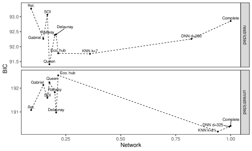
Figure 13: Relationship between network density and BIC value for the network-specific optimal GNAR model for the restricted and unrestricted data set

D.2 GNAR coefficient development for the optimal model: restricted versus unrestricted phase

The GNAR model $GNAR(\alpha=5,\beta=(1,1,1,1,0))$ for the KNN network $k=21$, optimal on the entire data set, is fitted on the data for the restricted and unrestricted phases. The absolute value for $\alpha$ and $\beta$ coefficients increase for the unrestricted pandemic phase compared to the restricted phase.

D.3 Prediction with GNAR models

The predictive accuracy of the best performing model, fitted on the entire COVID-19 data set for each COVID-19 network, is measured by predicting the lag-1 COVID-19 ID for the time period of 10 weeks, and computing the corresponding weekly mean absolute squared error (MASE) [103, 43, 38].

Figures 15 include the MASE for the county-specific ARIMA(2,1,0) models as a comparative benchmark. The ARIMA models are comparable to any GNAR model in predictive accuracy. No network performs visibly better than any other over space and time. The predictive performance for the Relative neighbourhood, SOI, Gabriel and Delaunay triangulation network is almost identical, which may have been expected due to their similar network characteristics.

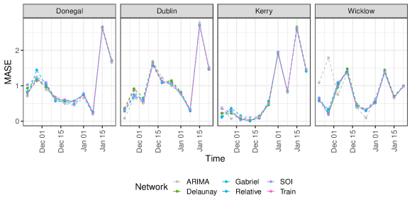
(a) Delaunay triangulation, Gabriel, Relative neighbourhood, SOI and Railway-based network

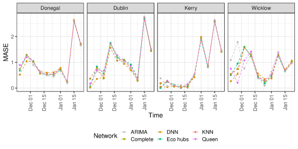
(b) KNN, DNN, Complete, Queen’s contiguity and Economic hub network

Figure 15: MASE values for COVID-19 network, as well as for the county-specific ARIMA benchmark models

While the general fit may not be unreasonable, we find that GNAR models across networks do not pick up on the many peaks and dips in the COVID-19 data, as evident from plotting the predicted COVID-19 ID for each network against the true COVID-19 ID in Figures 16 and 17. The Figures also include predictions based on the ARIMA model, fitted to each county separately. The predictive accuracy for the ARIMA models does not systematically surpass the GNAR models.

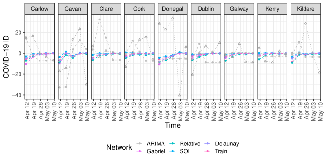
(a) Delaunay triangulation, Gabriel, Relative neighbourhood, SOI and Railway-based network

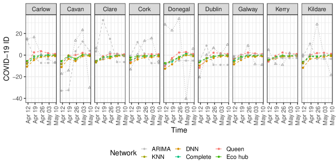
(b) KNN, DNN, Complete, Queen’s contiguity and Economic hub network

Figure 16: Predicted COVID-19 ID for the restricted phase; true values in dotted grey with triangles.

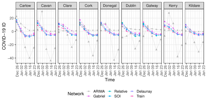
(a) Delaunay triangulation, Gabriel, Relative neighbourhood, SOI and Railway-based network

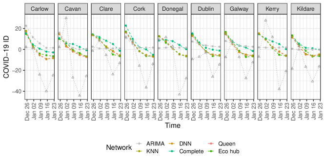
(b) KNN, DNN, Complete, Queen’s contiguity and Economic hub network

Figure 17: Predicted COVID-19 ID for the unrestricted phase; true values in dotted grey with triangles.

D.4 Gaussianity of residuals for GNAR models

The Gaussianity of the residuals may be statistically tested in a Kolmogorov-Smirnov test. Table 6 summarizes the fit of the GNAR model for the restricted and unrestricted data set for each county, including the p-value for the Kolmogorov-Smirnov test.

	Restricted			Unrestricted
County	$\bar{\varepsilon}$	av. MASE	p	$\bar{\varepsilon}$	av. MASE	p
Carlow	5.61 (12.73)	1.61 (1.41)	0.31	-16.3 (10.66)	1.14 (0.74)	0.00
Cavan	-3.26 (22.44)	0.82 (0.32)	0.03	-13.6 (24.81)	0.81 (0.32)	0.00
Clare	2.53 (5.64)	0.8 (0.93)	0.31	-10.54 (8.14)	0.8 (0.62)	0.00
Cork	2.85 (11.83)	0.77 (0.48)	0.09	-10.79 (12.59)	0.66 (0.65)	0.00
Donegal	12.57 (32.78)	0.86 (0.41)	0.00	-11.4 (18.06)	0.76 (0.88)	0.03
Dublin	1.48 (9.18)	0.68 (0.49)	0.01	-12.95 (8.87)	1.26 (0.86)	0.00
Galway	-1.74 (7.33)	0.75 (0.48)	0.04	-10.54 (11.14)	0.71 (0.58)	0.00
Kerry	-0.92 (7.26)	0.82 (0.56)	0.31	-8.91 (22.48)	0.69 (0.33)	0.03
Kildare	3.7 (17.37)	0.59 (0.68)	0.28	-15.55 (11.92)	0.89 (0.69)	0.00
Kilkenny	4.44 (0.98)	2.87 (0.64)	0.00	-16.61 (25.33)	0.76 (0.26)	0.00
Laois	-14.45 (9.72)	1.78 (1.2)	0.00	-15.97 (18.04)	0.66 (0.59)	0.01
Leitrim	0.61 (28.49)	1 (0.43)	0.03	-13.51 (14.88)	0.57 (0.62)	0.00
Limerick	6.8 (13.34)	0.94 (0.57)	0.03	-14.73 (12.21)	0.85 (0.61)	0.00
Longford	-9.78 (26.98)	0.78 (0.42)	0.03	-9.16 (12.54)	0.66 (0.79)	0.03
Louth	-2.42 (17.65)	0.52 (0.21)	0.03	-15.86 (4.7)	2.86 (0.85)	0.00
Mayo	-4.32 (8.03)	0.89 (0.63)	0.03	-9.46 (13.35)	0.67 (0.33)	0.00
Meath	-0.37 (4.34)	0.42 (0.35)	0.20	-10.94 (14.31)	0.58 (0.51)	0.00
Monaghan	2.44 (17.9)	0.6 (0.36)	0.03	-11.28 (4.76)	1.71 (0.72)	0.00
Offaly	-13.89 (13)	0.86 (0.81)	0.00	-11.14 (16.72)	0.89 (0.4)	0.00
Roscommon	15.06 (22.46)	0.86 (0.99)	0.03	-10.1 (23.85)	0.54 (0.4)	0.03
Sligo	-1.6 (17.31)	0.64 (0.46)	0.00	-15.05 (30.06)	0.56 (0.55)	0.03
Tipperary	-1.35 (31.3)	0.89 (0.34)	0.03	-14.83 (17.33)	0.8 (0.32)	0.00
Waterford	1.92 (6.47)	0.68 (0.38)	0.03	-20.78 (13.06)	1.11 (0.7)	0.00
Westmeath	-0.35 (26.33)	0.67 (0.44)	0.03	-13.83 (13.25)	0.82 (0.72)	0.00
Wexford	2.85 (16.66)	0.95 (0.78)	0.03	-14.18 (11.26)	1.04 (0.56)	0.00
Wicklow	-3.52 (11.49)	0.72 (0.4)	0.03	-11.96 (6.07)	1.27 (0.65)	0.00

Table 6: Average residual $\bar{\varepsilon}$ and average (av.) MASE value with standard deviation in brackets (.), as well as Kolmogorov-Smirnov p-value (p) for each county for restricted and unrestricted pandemic phase

The conclusions based on the Kolmogorov-Smirnov tests are verified by inspecting QQ-plots. The residual QQ-plots, which we show for the county Dublin as an illustration, indicate non-Gaussian residuals for the GNAR models across all networks, see Figure 18. This conclusion is corroborated when applying the Kolmogorov-Smirnov test across counties. The residual variance is low for time periods with low 1-lag COVID-19 ID and high for time periods with high 1-lag COVID-19 ID. Thus there may be some heteroscedastic noise in the data.

(a) Delaunay

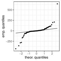
(b) Gabriel

(c) SOI

(d) Relative neighbourhood

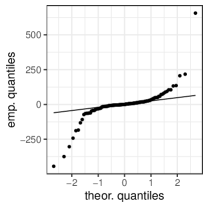
(e) Queen

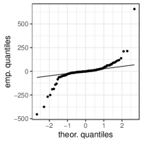
(f) Economic hub

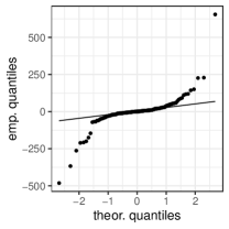
(g) Railway-based

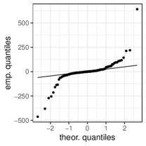
(h) KNN $k=21$

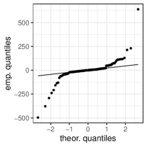
(i) DNN $d=325$

(j) Complete

Figure 18: QQ-plot for the residuals from the best performing GNAR models for county Dublin for each network on the entire COVID-19 data set

In contrast to the combined data set, when separating the data set into restricted and unrestricted phases of the pandemic, the QQ-plots for each GNAR model indicate Gaussian residuals for the restricted pandemic phases and residuals which deviate from the normal distribution for the unrestricted pandemic phases. The QQ-plots are shown in Figure 19 for the counties Dublin, Carlow and Cavan; the remaining counties show similar residual plots.

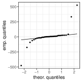
(a) Restricted

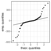
(b) Unrestricted

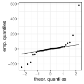
(c) Restricted

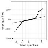
(d) Unrestricted

Figure 19: QQ-plot for the residuals from the best performing GNAR model and network for restricted and unrestricted pandemic phase for county Carlow (left) and Cavan (right)

Appendix E Simulation

To establish how well the GNAR model in general can reconstruct the data generating method, data is simulated according to the GNAR-5-21111 model on the Queen’s contiguity network. Choosing $s=(2,1,1,1,1)$, iid. error term $\varepsilon_{i,t}\sim N(0,\sigma^{2})$ with $\sigma^{2}=0.01$ and $\sigma^{2}=0.001$ and SPL weights, i.e. $\omega_{i,q}=\frac{1}{|N^{(r)}(i)|}$ where $|N^{(r)}(i)|$ denotes the number of vertices in the $r^{\,th}$-stage neighbourhood for $i$ and the first 5 time points are initialized as $X_{i,t}\sim N(10,\sigma^{2})$ iid., the outcome $X_{i}$ for county $i$ and timesteps $t=6,\dots,1000$ follows from

$$X_{i,t}=\sum_{j=1}^{5}\left(\alpha_{i,j}X_{i,t-j}+\sum_{r=1}^{s_{j}}\sum_{q\in N^{(r)}(i)}\beta_{j,r}\,\omega_{i,q}\,X_{q,t-j}\right)+\varepsilon_{i,t}$$

The simulated data is leveraged to train a GNAR model on the Queen’s contiguity network. Tables 7 ($\sigma^{2}=0.01$) and 8 ($\sigma^{2}=0.001$) compare the true and estimated GNAR model coefficients. The estimated confidence interval contains the true coefficient value only for no coefficient in the setting $\sigma^{2}=0.01$ and for one coefficients, $\alpha_{4}$, in the setting $\sigma^{2}=0.001$. Despite small noise, the GNAR model is incapable of correctly detecting the temporal and spatial dependence in the simulated data.

Coefficient	real value	re-computed value [95% CI]
$\alpha_{1}$	0.18	0.22 [0.21, 0.23]
$\beta_{1,1}$	0.14	0.01 [-0.01, 0.03]
$\beta_{1,2}$	0.41	-0.04 [-0.06, -0.02]
$\alpha_{2}$	-0.19	-0.02 [-0.03, -0.01]
$\beta_{2,1}$	-0.07	-0.05 [-0.06, -0.03]
$\alpha_{3}$	-0.09	0.26 [0.25, 0.27]
$\beta_{3,1}$	0.03	-0.03 [-0.04, -0.01]
$\alpha_{4}$	-0.17	0.17 [0.15, 0.18]
$\beta_{4,1}$	0.14	0.02 [0.01, 0.04]
$\alpha_{5}$	-0.11	0.09 [0.08, 0.1]
$\beta_{5,1}$	0.01	-0.02 [-0.03, -0.01]

Table 7: Coefficients for the GNAR model serving the data simulation and their re-computed values after fitting the GNAR model to the simulated data and their 95% confidence interval (CI) for the Queen’s contiguity network; the variance for the random error is set to $\sigma^{2}=0.01$.

Coefficient	real value	re-computed value [95% CI]
$\alpha_{1}$	0.18	-0.04 [-0.05, -0.03]
$\beta_{1,1}$	0.14	0 [-0.02, 0.01]
$\beta_{1,2}$	0.41	0.04 [0.02, 0.06]
$\alpha_{2}$	-0.19	-0.08 [-0.09, -0.07]
$\beta_{2,1}$	-0.07	-0.11 [-0.12, -0.1]
$\alpha_{3}$	-0.09	0 [-0.01, 0.01]
$\beta_{3,1}$	0.03	-0.08 [-0.09, -0.07]
$\alpha_{4}$	-0.17	-0.18 [-0.19, -0.17]
$\beta_{4,1}$	0.14	0.03 [0.02, 0.04]
$\alpha_{5}$	-0.11	0.21 [0.2, 0.22]
$\beta_{5,1}$	0.01	-0.03 [-0.04, -0.02]

Table 8: Coefficients for the GNAR model serving the data simulation and their re-computed values after fitting the GNAR model to the simulated data and their 95% confidence interval (CI) for the Queen’s contiguity network; the variance for the random error is set to $\sigma^{2}=0.001$.

References

- [1] Marina Knight, Kathryn Leeming, Guy Nason and Matthew Nunes “Generalised Network Autoregressive Processes and the GNAR package” In arXiv preprint arXiv:1912.04758, 2019
- [2] Marina Knight, Matthew Nunes and Guy Nason “Modelling, Detrending and Decorrelation of Network Time series” In arXiv preprint arXiv:1603.03221, 2016
- [3] Patrick Urrutia, David Wren, Chrysafis Vogiatzis and Ruriko Yoshida “SARS-CoV-2 Dissemination Using a Network of the US Counties” In Operations Research Forum 3, 2022, pp. 1–23 Springer
- [4] Pierre Nouvellet et al. “Reduction in mobility and COVID-19 transmission” In Nature communications 12.1 Nature Publishing Group UK London, 2021, pp. 1090
- [5] Jayson Jia et al. “Population flow drives spatio-temporal distribution of COVID-19 in China” In Nature 582.7812 Nature Publishing Group, 2020, pp. 389–394
- [6] Moritz Kraemer et al. “The effect of human mobility and control measures on the COVID-19 epidemic in China” In Science 368.6490 American Association for the Advancement of Science, 2020, pp. 493–497
- [7] Tao Li, Lili Rong and Anming Zhang “Assessing regional risk of COVID-19 infection from Wuhan via high-speed rail” In Transport Policy 106 Elsevier, 2021, pp. 226–238
- [8] Baichuan Mo et al. “Modeling epidemic spreading through public transit using time-varying encounter network” In Transportation Research Part C: Emerging Technologies 122 Elsevier, 2021, pp. 102893
- [9] Xiaoqian Sun, Sebastian Wandelt and Anming Zhang “On the degree of synchronization between air transport connectivity and COVID-19 cases at worldwide level” In Transport Policy 105 Elsevier, 2021, pp. 115–123
- [10] Joseph Wu, Kathy Leung and Gabriel Leung “Nowcasting and forecasting the potential domestic and international spread of the 2019-nCoV outbreak originating in Wuhan, China: a modelling study” In The Lancet 395.10225 Elsevier, 2020, pp. 689–697
- [11] Health Protection Surveillance Centre “Epidemiology of COVID-19 in Ireland - Dashboard” Accessed: 2023-03-20, https://epi-covid-19-hpscireland.hub.arcgis.com, 2022
- [12] Health Protection Surveillance Centre “Summary of COVID-19 virus variants in Ireland” Accessed: 2022-07-22, https://www.hpsc.ie/a-z/respiratory/coronavirus/novelcoronavirus/surveillance/summaryofcovid-19virusvariantsinireland/, 2022
- [13] Government of Ireland “Ireland’s COVID-19 Data Hub” Accessed: 2023-01-23, https://covid-19.geohive.ie, 2022
- [14] Ordnance Survey Ireland “Covid-19 HPSC County Statistics Historic Data” Accessed: 2022-06-18 Irish government’s open data portal DATA.GOV.IE, https://data.gov.ie/dataset/covid-19-hpsc-county-statistics-historic-data?package_type=dataset, 2022
- [15] Central Statistics Office “2016 Census Forms” Accessed: 2022-07-06, https://www.cso.ie/en/census/2016censusforms/, 2016
- [16] Jakub Kubiczek and BartŁomiej Hadasik “Challenges in Reporting the COVID-19 Spread and its Presentation to the Society” In Journal of Data and Information Quality (JDIQ) 13.4 ACM New York, NY, 2021, pp. 1–7
- [17] Gino Sartor et al. “COVID-19 in Italy: Considerations on official data” In International Journal of Infectious Diseases 98 Elsevier, 2020, pp. 188–190
- [18] Health Protection Surveillance Centre “First year of the COVID-19 pandemic in Ireland” Accessed: 2022-06-23, https://www.hpsc.ie/a-z/respiratory/coronavirus/novelcoronavirus/casesinireland/covid-19annualreports/, 2021
- [19] Health Protection Surveillance Centre “Weekly report on the epidemiology of COVID-19 in Ireland - Week 24, 2022” Accessed: 2022-06-28, https://www.hpsc.ie/a-z/respiratory/coronavirus/novelcoronavirus/surveillance/epidemiologyofcovid-19inirelandweeklyreports/, 2022
- [20] William Wei “Time series analysis” Redwood City, California; Wokingham: Addison-Wesley, 2006
- [21] Colin Brennan “A year with Covid in Ireland - timeline of incredible lockdowns, cases and deaths, pub closures and disasters” Accessed: 2022-07-22 The Irish Mirror, https://www.irishmirror.ie/news/irish-news/year-covid-ireland-timeline-incredible-23585166, 2022
- [22] Independent - Documentary 01.03.2022 “Timeline: Two years of Covid-19 in Ireland - Video” Accessed: 2022-07-22, https://www.youtube.com/watch?v=BF6oLSwKMF0, 2022
- [23] Elaine Loughlin “Timeline of a pandemic: How Covid-19 changed our way of life” Accessed: 2022-07-22 The Irish Examiner, https://www.irishexaminer.com/news/arid-40790595.html, 2022
- [24] Cormac McQuinn, Barry Roche and Paul Cullen “Ireland reopens: inter-county travel resumes as hairdressers and non-essential retail return” Accessed: 2023-02-02 The Irish Times, https://www.irishtimes.com/news/politics/ireland-reopens-inter-county-travel-resumes-as-hairdressers-and-non-essential-retail-return-1.4559937, 2021
- [25] Vittoria Colizza, Alain Barrat, Marc Barthélemy and Alessandro Vespignani “The role of the airline transportation network in the prediction and predictability of global epidemics” In Proceedings of the National Academy of Sciences 103.7 National Acad Sciences, 2006, pp. 2015–2020
- [26] M Sawada “Global Spatial Autocorrelation Indices - Moran’s I, Geary’s C and the General Cross-Product Statistic” Accessed: 2022-06-28, http://www.lpc.uottawa.ca/publications/moransi/moran.htm, 2022
- [27] Richard Gardham “The five largest cities in Ireland (and their investment strengths)” Accessed: 2022-07-06 Investmentmonitor, https://www.investmentmonitor.ai/analysis/ireland-largest-cities-investment-dublin, 2022
- [28] Eric W Weisstein “Great circle” Accessed: 2022-07-06 In https://mathworld.wolfram.com/ Wolfram Research, Inc., 2002
- [29] Roger Bivand “R Packages for Analyzing Spatial Data: A Comparative Case Study with Areal Data” Accessed: 2022-07-22 In Geographical Analysis, https://doi.org/10.1111/gean.12319, 2022
- [30] David Eppstein, Michael Paterson and Frances Yao “On nearest-neighbor graphs” In Discrete & Computational Geometry 17.3 Springer, 1997, pp. 263–282
- [31] Roger Bivand, Pebesma Edzer and Gomez-Rubio Virgilio “Applied Spatial Data Analysis with R” Accessed: 2022-07-22 New York: Springer, https://r-spatial.github.io/spdep/MISCs/nb.html, 2013
- [32] Long Chen and Jin-chao Xu “Optimal Delaunay Triangulations” In Journal of Computational Mathematics JSTOR, 2004, pp. 299–308
- [33] Shweta Bansal, Bryan Grenfell and Lauren Ancel Meyers “When individual behaviour matters: homogeneous and network models in epidemiology” In Journal of the Royal Society Interface 4.16 The Royal Society London, 2007, pp. 879–891
- [34] Xuening Zhu et al. “Network Vector Autoregression” In The Annals of Statistics 45.3 Institute of Mathematical Statistics, 2017, pp. 1096–1123
- [35] George Box, Gwilym Jenkins, Gregory Reinsel and Greta Ljung “Time series analysis: Forecasting and Control” Chichester: John Wiley & Sons, 2015
- [36] James Douglas Hamilton “Time Series Analysis” Princeton, New Jersey: Princeton University Press, 2020
- [37] R Package Documentation “GNAR source code” Accessed: 2022-07-14, https://rdrr.io/cran/GNAR/f/, 2022
- [38] Kathryn Leeming “New Methods in Time Series Analysis: Univariate Testing and Network Autoregression Modelling”, 2019
- [39] Helmut Lütkepohl “Introduction to Multiple Time Series Analysis” Berlin, London: Springer-Verlag, 1991
- [40] Gideon Schwarz “Estimating the dimension of a model” In The Annals of Statistics JSTOR, 1978, pp. 461–464
- [41] Helmut Lütkepohl “New introduction to multiple Time Series Analysis” Berlin: Springer Science & Business Media, 2005
- [42] Jinchi Lv and Jun S Liu “Model selection principles in misspecified models” In Journal of the Royal Statistical Society: Series B: Statistical Methodology JSTOR, 2014, pp. 141–167
- [43] Rob Hyndman and Anne Koehler “Another look at measures of forecast accuracy” In International Journal of Forecasting 22.4 Elsevier, 2006, pp. 679–688
- [44] Douglas C Montgomery, Cheryl L Jennings and Murat Kulahci “Introduction to Time Series Analysis and Forecasting” Chichester: John Wiley & Sons, 2015
- [45] Anna Broido and Aaron Clauset “Scale-free networks are rare” In Nature Communications 10.1 Nature Publishing Group, 2019, pp. 1–10
- [46] Mark Newman “Power laws, Pareto distributions and Zipf’s law” In Contemporary Physics 46.5 Taylor & Francis, 2005, pp. 323–351
- [47] Andrew David Cliff and Keith Ord “Spatial Processes: Models & Applications” London: Pion, 1981
- [48] Patrick Moran “Notes on continuous stochastic phenomena” In Biometrika 37.1/2 JSTOR, 1950, pp. 17–23
- [49] Xiaobo Zhou and Henry Lin “Moran’s I” Boston, MA: Springer US, 2008, pp. 725–725
- [50] Central Statistics Office “Urban and Rural Life in Ireland, 2019” Accessed: 2022-07-12, https://www.cso.ie/en/releasesandpublications/ep/p-howpublishedi/urbanandrurallifeinireland2019/introduction/, 2022
- [51] Michele Coscia “Pearson correlations on complex networks” In Journal of Complex Networks 9.6 Oxford University Press, 2021, pp. cnab036
- [52] Melika Lotfi, Michael Hamblin and Nima Rezaei “COVID-19: Transmission, prevention, and potential therapeutic opportunities” In Clinica Chimica Acta 508 Elsevier, 2020, pp. 254–266
- [53] Department of the Taoiseach “Resilience and Recovery 2020-2021: Plan for Living with COVID-19” Accessed: 2022-06-23, https://www.gov.ie/en/publication/e5175-resilience-and-recovery-2020-2021-plan-for-living-with-covid-19/, 2020
- [54] Yanding Wang et al. “Prediction and analysis of COVID-19 daily new cases and cumulative cases: times series forecasting and machine learning models” In BMC Infectious Diseases 22.1 Springer, 2022, pp. 1–12
- [55] Josh A Firth et al. “Combining fine-scale social contact data with epidemic modelling reveals interactions between contact tracing, quarantine, testing and physical distancing for controlling COVID-19” In MedRxiv Cold Spring Harbor Laboratory Press, 2020, pp. 2020–05
- [56] Cliodhna O’Connor et al. “Bordering on crisis: A qualitative analysis of focus group, social media, and news media perspectives on the Republic of Ireland-Northern Ireland border during the ‘first wave’of the COVID-19 pandemic” In Social Science & Medicine 282 Elsevier, 2021, pp. 114111
- [57] Houses of the Oireachtas “Dáil Éireann debate - Thursday, 7 May 2020” Accessed: 2023-03-14, https://www.oireachtas.ie/en/debates/debate/dail/2020-05-07/2/spk_38, 2020
- [58] Greta M Ljung and George EP Box “On a measure of lack of fit in time series models” In Biometrika 65.2 Oxford University Press, 1978, pp. 297–303
- [59] Andrea Bertozzi et al. “The challenges of modeling and forecasting the spread of COVID-19” In Proceedings of the National Academy of Sciences 117.29 National Acad Sciences, 2020, pp. 16732–16738
- [60] John Ioannidis, Sally Cripps and Martin Tanner “Forecasting for COVID-19 has failed” In International Journal of Forecasting Elsevier, 2020
- [61] Ruiyun Li et al. “Substantial undocumented infection facilitates the rapid dissemination of novel coronavirus (SARS-CoV-2)” In Science 368.6490 American Association for the Advancement of Science, 2020, pp. 489–493
- [62] Eurostat - Statistics explained “Glossary: Modal split of passenger transport” Accessed: 2022-07-12, https://ec.europa.eu/eurostat/statistics-explained/index.php?title=Glossary:Modal_split_of_passenger_transport, 2022
- [63] Statistics Finland “Definition: Passenger-kilometre” Accessed: 2022-07-12, https://www.stat.fi/meta/kas/henkilo_km_en.html, 2022
- [64] Eurostat - Data Explorer “Modal split of passenger transport” Accessed: 2022-07-12, https://appsso.eurostat.ec.europa.eu/nui/show.do?dataset=tran_hv_psmod&lang=en, 2021
- [65] Department of Transport “Transport Trends 2021 - An Overview of Ireland’s Transport Sector” Accessed: 2022-07-12, https://www.gov.ie/en/publication/182bd-transport-trends-2021/, 2022
- [66] COVID-19 Community Mobility Report “Mobility changes - Ireland 21 July 2022” Accessed: 2022-07-25, https://www.gstatic.com/covid19/mobility/2022-07-21_IE_Mobility_Report_en-GB.pdf, 2022
- [67] Ruben Gabriel and Robert Sokal “A new statistical approach to geographic variation analysis” In Systematic Zoology 18.3 Society of Systematic Zoology, 1969, pp. 259–278
- [68] Frank Harary, Michael Jacobson, Marc Lipman and Fred McMorris “Abstract sphere-of-influence graphs” In Mathematical and Computer Modelling 17.11 Elsevier, 1993, pp. 77–83
- [69] Jing Zhou, Dong Li, Rui Pan and Hansheng Wang “Network GARCH model” In Statistica Sinica 30.4 JSTOR, 2020, pp. 1723–1740
- [70] Raymond Myers, Douglas Montgomery and Geoffrey Vining “Generalized Linear Models : with Applications in Engineering and the Sciences”, Wiley series in Probability and Statistics New York, NY: Wiley, 2002
- [71] Trevor Hastie, Robert Tibshirani and J Friedman “The Elements of Statistical Learning : Data Mining, Inference, and Prediction”, Springer Series in Statistics New York: Springer, 2009
- [72] Raphael Rehms et al. “A Bayesian hierarchical approach to account for reporting uncertainty, variants of concern and vaccination coverage when estimating the effects of non-pharmaceutical interventions on the spread of infectious diseases” In medRxiv Cold Spring Harbor Laboratory Press, 2022, pp. 2022–06
- [73] Seth Flaxman et al. “Estimating the effects of non-pharmaceutical interventions on COVID-19 in Europe” In Nature 584.7820 Nature Publishing Group, 2020, pp. 257–261
- [74] Janoś Gabler, Tobias Raabe, Klara Röhrl and Hans-Martin von Gaudecker “The effectiveness of testing, vaccinations and contact restrictions for containing the COVID-19 pandemic” In Scientific Reports 12.1 Nature Publishing Group, 2022, pp. 1–8
- [75] Tom Britton et al. “Stochastic epidemic models with inference” Springer, 2019
- [76] Christopher E Overton et al. “Using statistics and mathematical modelling to understand infectious disease outbreaks: COVID-19 as an example” In Infectious Disease Modelling 5 Elsevier, 2020, pp. 409–441
- [77] Gordon L Nichols et al. “Coronavirus seasonality, respiratory infections and weather” In BMC Infectious Diseases 21.1 BioMed Central, 2021, pp. 1–15
- [78] Robert Shumway, David Stoffer and David Stoffer “Time Series Analysis and its Applications” New York: Springer, 2000
- [79] Christopher Manzira, Anna Charly and Brian Caulfield “Assessing the impact of mobility on the incidence of COVID-19 in Dublin City” In Sustainable Cities and Society 80 Elsevier, 2022, pp. 103770
- [80] Nicola Perra et al. “Random walks and search in time-varying networks” In Physical Review Letters 109.23 APS, 2012, pp. 238701
- [81] Thomas Chaney “The gravity equation in international trade: An explanation” In Journal of Political Economy 126.1 University of Chicago Press Chicago, IL, 2018, pp. 150–177
- [82] Foo Chee “Vodafone, Deutsche Telekom, 6 other telcos to help EU track virus” Accessed: 2022-07-06 Reuters, https://www.reuters.com/article/us-health-coronavirus-telecoms-eu-idUSKBN21C36G, 2020
- [83] European Parliament “Tracking mobile devices to fight coronavirus” Accessed: 2022-07-06, https://www.europarl.europa.eu/RegData/etudes/BRIE/2020/649384/EPRS_BRI(2020)649384_EN.pdf, 2020
- [84] Alun Lloyd and Steve Valeika “Network models in epidemiology: an overview” In Complex population dynamics: nonlinear modeling in ecology, epidemiology and genetics World Scientific, 2007, pp. 189–214
- [85] Mark Newman “Networks” Oxford: Oxford University Press, 2018
- [86] Keith Ord “Estimation methods for models of spatial interaction” In Journal of the American Statistical Association 70.349 Taylor & Francis, 1975, pp. 120–126
- [87] Patrick Doreian “Estimating linear models with spatially distributed data” In Sociological Methodology 12 JSTOR, 1981, pp. 359–388
- [88] Jesus Mur “Testing for spatial autocorrelation: moving average versus autoregressive processes” In Environment and Planning A 31.8 SAGE Publications Sage UK: London, England, 1999, pp. 1371–1382
- [89] Roger Leenders “Modeling social influence through network autocorrelation: constructing the weight matrix” In Social Networks 24.1 Elsevier, 2002, pp. 21–47
- [90] Patrick Doreian “Linear models with spatially distributed data: Spatial disturbances or spatial effects?” In Sociological Methods & Research 9.1 Sage Publications Sage CA: Thousand Oaks, CA, 1980, pp. 29–60
- [91] Patrick Doreian “Network autocorrelation models: Problems and prospects” In Spatial statistics: Past, present, future Michigan Document Services Ann Arbor, 1989, pp. 369–89
- [92] Patrick Doreian, L Freeman, D White and A Romney “Models of network effects on social actors” In Research Methods in Social Network Analysis George Mason University Press Fairfax, VA, 1989, pp. 295–317
- [93] Malcolm Dow, Michael Burton and Douglas White “Network autocorrelation: A simulation study of a foundational problem in regression and survey research” In Social Networks 4.2, 1982, pp. 169–200
- [94] Colin Loftin and Sally Ward “A spatial autocorrelation model of the effects of population density on fertility” In American Sociological Review JSTOR, 1983, pp. 121–128
- [95] Douglas White, Michael Burton and Malcolm Dow “Sexual division of labor in African agriculture: a network autocorrelation analysis” In American Anthropologist 83.4 Wiley Online Library, 1981, pp. 824–849
- [96] Jude C Hays, Aya Kachi and Robert Franzese Jr. “A spatial model incorporating dynamic, endogenous network interdependence: A political science application” In Statistical Methodology 7.3 Elsevier, 2010, pp. 406–428
- [97] Binyan Jiang, Jailing Li and Qiwei Yao “Autoregressive networks” In arXiv preprint arXiv:2010.04492, 2020
- [98] Xuening Zhu, Weining Wang, Hansheng Wang and Wolfgang Karl Härdle “Network Quantile Autoregression” In Journal of Econometrics 212.1 Elsevier, 2019, pp. 345–358
- [99] Xuening Zhu and Rui Pan “Grouped Network Vector Autoregression” In Statistica Sinica 30.3 JSTOR, 2020, pp. 1437–1462
- [100] Guy Nason and James Wei “Quantifying the economic response to COVID-19 mitigations and death rates via forecasting Purchasing Managers’ Indices using Generalised Network Autoregressive models with exogenous variables” In arXiv preprint arXiv:2107.07605, 2021
- [101] Hirotugu Akaike “A new look at the statistical model identification” In IEEE Transactions on Automatic Control 19.6 Ieee, 1974, pp. 716–723
- [102] Hamparsum Bozdogan “Model selection and Akaike’s information criterion (AIC): The general theory and its analytical extensions” In Psychometrika 52.3 Springer, 1987, pp. 345–370
- [103] Ludwig Fahrmeir et al. “Statistik: Der Weg zur Datenanalyse” Berlin, London: Springer-Verlag, 2016