Relativistic second-order viscous hydrodynamics from kinetic theory with extended relaxation-time approximation

Abstract

We use the extended relaxation time approximation for the collision kernel, which incorporates a particle-energy dependent relaxation time, to derive second-order viscous hydrodynamics from the Boltzmann equation for a system of massless particles. The resulting transport coefficients are found to be sensitive to the energy dependence of the relaxation time and have significant influence on the fluid’s evolution. Using the derived hydrodynamic equations, we study the evolution of a fluid undergoing (0+1)-dimensional expansion with Bjorken symmetry and investigate the fixed point structure inherent in the equations. Further, by employing a power law parametrization to describe the energy dependence of the relaxation time, we successfully reproduce the stable free-streaming fixed point for a specific power of the energy dependence. The impact of the energy-dependent relaxation time on the processes of isotropization and thermalization of an expanding plasma is discussed.

I Introduction

The relativistic Boltzmann equation is a transport equation that governs the space-time evolution of the single-particle phase-space distribution function. It is capable of accurately describing the collective dynamics of the system in the limit of small mean free path and therefore has been employed extensively to formulate the theory of relativistic hydrodynamics Muronga (2007); York and Moore (2009); Betz et al. (2009); Romatschke (2010); Denicol et al. (2012); Florkowski et al. (2013); Weickgenannt et al. (2021). However, solving the Boltzmann equation directly is challenging due to the complicated integro-differential nature of the collision term, which involves the integral of the product of distribution functions. Over several decades, various approximations have been proposed to simplify the collision term in the linearized regime. In 1969, following earlier works by Bhatnagar-Gross-Krook Bhatnagar et al. (1954) and Welander Welander (1954), Marle introduced a relaxation time approximation for non-relativistic systems Marle (1969). However, Marle’s version was not applicable to massless particles and was ill-defined in the relativistic limit. Anderson and Witting resolved these issues by generalizing Marle’s model to the relativistic regime, qualitatively recovering the results obtained using Grad’s method of moments in the relativistic limit Anderson and Witting (1974). These models, introduced by Marle and Anderson-Witting, incorporate a collision time scale known as the relaxation time. The Anderson-Witting model requires the relaxation time to be independent of particle momenta, making it straightforward to apply in the formulation of relativistic dissipative hydrodynamics.

The Anderson-Witting model achieves enormous simplification by approximating that collisions drive the system towards local equilibrium exponentially without explicitly describing the interaction mechanism of the microscopic constituents. This approximation provides a highly accurate description of the collective dynamics for systems close to equilibrium. In the following, we will refer to the Anderson-Witting model as the relaxation-time approximation (RTA). Despite its simplistic nature, RTA and its variations have proven to be immensely useful and have been extensively employed in formulating relativistic dissipative hydrodynamics as well as in deriving transport coefficients Denicol et al. (2010); Jaiswal (2013a); Jaiswal et al. (2014); Mohanty et al. (2019); Kurian (2020); Gabbana et al. (2017); Bhadury et al. (2020); Panda et al. (2021); Vyas et al. (2023); Singha et al. (2023). Recently, it has also been applied to study the domain of applicability of hydrodynamics Heller et al. (2018); Blaizot and Yan (2018); Florkowski et al. (2018); Strickland (2018); Chattopadhyay et al. (2018); Kurkela et al. (2020); Blaizot and Yan (2020, 2021a); Dash and Roy (2020); Jaiswal et al. (2021); Soloviev (2022); Blaizot and Yan (2021b); Chattopadhyay et al. (2022); Jaiswal et al. (2022a, b); Chattopadhyay et al. (2023); Ambrus et al. (2023); Jankowski and Spaliński (2023). This simple model appears to capture effective microscopic interactions across a wide range of theories.

When deriving dissipative hydrodynamic equations from kinetic theory using the RTA approximation, it is typically assumed that the relaxation time is independent of particle energy (or momentum). Additionally, one is constrained to work in the Landau frame to ensure the preservation of macroscopic conservation laws. However, in realistic systems, the collision time scale generally depends on the microscopic interactions Dusling et al. (2010); Chakraborty and Kapusta (2011); Dusling and Schäfer (2012); Kurkela and Wiedemann (2019). Introducing an energy-dependent relaxation time leads to a violation of microscopic conservation laws in the Landau frame. As a result, there has been considerable interest in developing a consistent formulation of relativistic dissipative hydrodynamics with an energy-dependent relaxation-time approximation for the Boltzmann equation that satisfies both microscopic and macroscopic conservation laws Teaney and Yan (2014); Mitra (2021); Rocha et al. (2021); Dash et al. (2022).

Relativistic viscous hydrodynamics-based multistage dynamical models have demonstrated success in accurately describing a broad spectrum of soft hadronic observables in heavy-ion collisions Gale et al. (2013); Derradi de Souza et al. (2016); Schenke et al. (2020). The hydrodynamics stage of the evolution encompasses the deconfined quarks and gluons regime at high temperatures, the phase transition, and the hadron gas phase Heinz and Snellings (2013). The dynamical properties of the evolving non-equilibrium nuclear matter are governed by a set of transport coefficients, such as the shear and bulk viscosities Romatschke and Romatschke (2007); Song and Heinz (2008); Buchel and Pagnutti (2009); Denicol et al. (2009); Ryu et al. (2015). These transport coefficients play a crucial role in explaining the hadronic observables in heavy-ion collisions. Thus, a major goal of heavy-ion phenomenology is to extract the temperature dependence of these transport coefficients for the evolving nuclear matter, and considerable efforts have been made to determine these coefficients from various aspects. Most phenomenological studies adopt parameterized forms for the shear and bulk viscosities Akiba et al. (2015); Denicol et al. (2016); Vujanovic et al. (2018); Karmakar et al. (2023). Recent studies have employed Bayesian methods to obtain these parameters and have provided bounds on the transport coefficients Bernhard et al. (2015, 2016, 2019); Everett et al. (2021a); Nijs et al. (2021); Everett et al. (2021b). However, since these parametrizations do not stem from microscopic considerations, the predictability of such models is limited. Additionally, the second-order transport coefficients utilized in these hydrodynamic models are obtained for specific interactions, and, as a result, they may fail to accurately capture the system’s behavior during its evolution.

In our recent work Dash et al. (2022), we presented a framework for the consistent derivation of relativistic dissipative hydrodynamics from the Boltzmann equation, incorporating a particle energy-dependent relaxation time by extending the Anderson-Witting relaxation-time approximation. Within this extended RTA (ERTA) framework, we derived the first-order hydrodynamic equations and demonstrated that the hydrodynamic transport coefficients can exhibit significant variations with the energy dependence of the relaxation time. Notably, the ERTA framework allows for the adjustment of interaction characteristics by tuning the energy dependence of the relaxation time, enabling a partial description of the transition from deconfined quark-gluon plasma at high temperatures to a weakly interacting gas of hadrons at lower temperatures. While the formulation presented in Ref. Dash et al. (2022) successfully incorporates an energy-dependent relaxation time into the RTA, it still suffers from the well-known issue of acausality in first-order relativistic hydrodynamics within the Landau frame Hiscock and Lindblom (1983, 1985); Bemfica et al. (2018); Kovtun (2019); Bemfica et al. (2019); Hoult and Kovtun (2020); Gavassino et al. (2020); Hoult and Kovtun (2022); Biswas et al. (2022). Consequently, there is a need for a second-order theory that addresses this issue Israel (1976); Israel and Stewart (1979), allowing for its application in heavy-ion collision simulations.

In the present study, we employ the ERTA framework to derive second-order hydrodynamic equations in the Landau frame for a conformal system without conserved charges, incorporating an energy-dependent relaxation time. The second-order transport coefficients are found to be sensitive to the energy dependence of the relaxation time. We focus on a boost-invariant flow in (0+1) dimensions and investigate the fixed point structure of the hydrodynamic equations. Our analysis reveals that the location of the free-streaming fixed points is influenced by the energy dependence of the relaxation time. By employing a power law parametrization to describe this energy dependence, we successfully reproduce the stable free-streaming fixed point for a specific power of the energy dependence. Furthermore, we explore the impact of the energy-dependent relaxation time on the processes of isotropization and thermalization of a boost invariant expanding plasma.

This paper is organized as follows: In Sec. II we review the basic hydrodynamic equations for a conformal, chargeless fluid. Sec. III briefly summarizes the results of Ref. Dash et al. (2022) and outlines the steps necessary to derive second-order hydrodynamic equations, which we present in Sec. IV. Appendix A contains the derivation of the results stated in Sec. IV.1. In Appendix B, we show that microscopic conservation holds till third order following the prescription outlined in Sec. IV. In Sec. V, we consider Bjorken flow and study the effect of the energy dependence of the relaxation time on systems’ thermalization. We summarize our results in Sec. VI.

II Overview

The energy-momentum tensor for a system of massless particles with no net conserved charge can be expressed in terms of the single-particle phase–space distribution function, $f(x,p)$, as

$$T^{\mu\nu}=\int\mathrm{dP}\,p^{\mu}p^{\nu}f={\cal E}u^{\mu}u^{\nu}-{\cal P}\Delta^{\mu\nu}+\pi^{\mu\nu},$$ (1)

where $\mathrm{dP}=d^{3}\vec{p}/\left[(2\pi)^{3}E_{p}\right]$ is the invariant momentum-space integration measure with $E_{p}$ representing the particle energy which is equal to the magnitude of the particle three-momenta for massless particles, $E_{p}=|\vec{p}|$. The projection operator $\Delta^{\mu\nu}=g^{\mu\nu}-u^{\mu}u^{\nu}$ is orthogonal to the hydrodynamic four-velocity $u^{\mu}$ defined in the Landau frame: $u_{\nu}T^{\mu\nu}={\cal E}u^{\mu}$, where ${\cal E}$ is the energy density. In the above equation, $\mathcal{P}$ is the thermodynamic pressure and $\pi^{\mu\nu}$ is the shear viscous stress. We work with the Minkowskian metric tensor $g^{\mu\nu}\equiv\mathrm{diag}(+,-,-,-)$.

The energy-momentum conservation $\partial_{\mu}T^{\mu\nu}=0$ yields the fundamental evolution equations for ${\cal E}$ and $u^{\mu}$ as,

$$\dot{\cal E}+({\cal E}+{\cal P})\theta-\pi^{\mu\nu}\sigma_{\mu\nu} =0,$$ (2)

$$({\cal E}+{\cal P})\dot{u}^{\alpha}-\nabla^{\alpha}{\cal P}+\Delta^{\alpha}_{\nu}\partial_{\mu}\pi^{\mu\nu} =0,$$ (3)

Here we use the standard notation $\dot{A}=u^{\mu}\partial_{\mu}A$ for co-moving derivatives, $\theta\equiv\partial_{\mu}u^{\mu}$ for the expansion scalar, $\sigma^{\mu\nu}\equiv\frac{1}{2}(\nabla^{\mu}u^{\nu}+\nabla^{\nu}u^{\mu})-\frac{1}{3}\theta\Delta^{\mu\nu}$ for the velocity stress tensor, and $\nabla^{\alpha}=\Delta^{\mu\alpha}\partial_{\mu}$ for space-like derivatives.

We consider the equilibrium momentum distribution function to have the Maxwell-Boltzmann distribution in the local rest frame of the fluid, $f_{\rm eq}=\exp\left[-(u\cdot p)/T\right]$. The equilibrium energy density then takes the form,

$${\cal E}_{0}=u_{\mu}u_{\nu}\int\mathrm{dP}\,p^{\mu}p^{\nu}f_{\rm eq}=\frac{3T^{4}}{\pi^{2}}.$$ (4)

For an out-of-equilibrium system, the temperature $T$ is an auxiliary quantity which we define using the matching condition ${\cal E}\equiv{\cal E}_{0}$. Also, the thermodynamic pressure and entropy density are given by,

$${\cal P} =-\frac{1}{3}\Delta_{\mu\nu}\int\mathrm{dP}\,p^{\mu}p^{\nu}f_{\rm eq}=\frac{T^{4}}{\pi^{2}}\,,$$ (5)

$${\cal S} =\frac{{\cal E}+{\cal P}}{T}=\frac{4T^{3}}{\pi^{2}}\,.$$ (6)

The evolution of temperature is obtained from the hydrodynamic equations of motion (2) and (3),

$$\dot{\beta} =\frac{\beta\theta}{3}-\frac{\beta}{3({\cal E}+{\cal P})}\pi^{\mu\nu}\sigma_{\mu\nu}\,,$$ (7)

$$\nabla^{\mu}\beta =-\beta\dot{u}^{\mu}-\frac{\beta}{{\cal E}+{\cal P}}\Delta^{\mu}_{\alpha}\partial_{\nu}\pi^{\alpha\nu}\,,$$ (8)

where $\beta=1/T$.

The non-equilibrium phase-space distribution function can be written as $f=f_{\rm eq}+\Delta f$, where $\Delta f$ represents the out-of-equilibrium correction to the distribution function. Using Eq. (1) the shear stress tensor $\pi^{\mu\nu}$ can be expressed in terms of $\Delta f$ as

$$\pi^{\mu\nu} =\Delta^{\mu\nu}_{\alpha\beta}\int\mathrm{dP}\,p^{\alpha}p^{\beta}\,\Delta f\,,$$ (9)

where $\Delta^{\mu\nu}_{\alpha\beta}\equiv\frac{1}{2}\left(\Delta^{\mu}_{\alpha}\Delta^{\nu}_{\beta}+\Delta^{\mu}_{\beta}\Delta^{\nu}_{\alpha}\right)-\frac{1}{3}\Delta^{\mu\nu}\Delta_{\alpha\beta}$ is a doubly symmetric and traceless projection operator orthogonal to $u^{\mu}$ as well as $\Delta^{\mu\nu}$. The evolution of the shear stress tensor depends on the evolution of the distribution function. In this work, we consider the evolution of the distribution function to be governed by the Boltzmann equation with the collision term, $\textfrak{C}[f]$, in the Extended Relaxation Time Approximation (ERTA) Teaney and Yan (2014); Dash et al. (2022),

$$p^{\mu}\partial_{\mu}f=\textfrak{C}[f]=-\frac{(u\cdot p)}{\tau_{\rm R}(x,p)}\left(f-f_{\rm eq}^{*}\right)\,,$$ (10)

where the relaxation time, $\tau_{\rm R}(x,p)$, may depend on the particle momenta. The equilibrium distribution function is considered to be of the Maxwell-Boltzmann form in the ‘thermodynamic frame’, $f_{\rm eq}^{*}=\exp\left[-\left(u^{*}\cdot p\right)/T^{*}\right]$. Here the thermodynamic frame is defined to be the local rest frame of a time-like four vector $u_{\mu}^{*}$ which need not necessarily correspond to the hydrodynamic four-velocity $u_{\mu}$, and $T^{*}$ is the temperature in the local rest frame of $u_{\mu}^{*}$ (see Ref. Dash et al. (2022) for a detailed discussion).

We briefly review the derivation of first-order shear stress from the above kinetic equation in the next section.

III First-order hydrodynamics

We employ Chapman-Enskog-like expansion about hydrodynamic equilibrium to iteratively solve the ERTA Boltzmann equation (10),

$$f=f_{\rm eq}+\delta f_{(1)}+\delta f_{(2)}+\delta f_{(3)}+\cdots$$ (11)

Here $\delta f_{(i)}$ represents the $i$th order gradient correction to the hydrodynamic equilibrium distribution function. The correction to the distribution function to the first order is

$$\delta f_{(1)}=\delta f^{*}_{(1)}+\frac{\tau_{\rm R}}{T}\frac{p^{\mu}p^{\nu}}{u\cdot p}\sigma_{\mu\nu}f_{\rm eq}\,,$$ (12)

where we have replaced the derivatives of temperature with the derivatives of fluid velocity using Eqs. (7,8) consistently keeping terms till first order in gradients, and have defined $\delta f^{*}\equiv f_{\rm eq}^{*}-f_{\rm eq}$. Defining $T^{*}\equiv T+\delta T$ and $u^{\mu}_{*}\equiv u^{\mu}+\delta u^{\mu}$, we obtain the first-order correction $\delta f_{(1)}^{*}$ by Taylor expanding $f_{\rm eq}^{*}$ about $u^{\mu}$ and $T$,

$$\delta f^{*}_{(1)}=\left(-\frac{(\delta u\cdot p)}{T}+\frac{(u\cdot p)\delta T}{T^{2}}\right)f_{\rm eq}\,.$$ (13)

Using Eqs. (12) and (13), the quantities $\delta u^{\mu}$ and $\delta T$ are obtained by imposing the Landau frame conditions, $u_{\nu}T^{\mu\nu}={\cal E}u^{\mu}$, and the matching condition, ${\cal E}={\cal E}_{0}$. We find that these quantities vanish for a system of massless and chargeless particles at first-order in gradients, and the resulting first-order correction is given by

$$\delta f_{(1)}=\frac{\tau_{\rm R}}{T}\frac{p^{\mu}p^{\nu}}{u\cdot p}\sigma_{\mu\nu}f_{\rm eq}\,.$$ (14)

It can be easily checked that the microscopic conservation of energy-momentum at first order holds by taking the first momentum-moment of the Boltzmann equation (10) with $f\mapsto f_{(1)}=f_{\rm eq}+\delta f_{(1)}$,

$$\partial_{\mu}\int\mathrm{dP}\,p^{\mu}p^{\nu}f_{(1)} =-\int\mathrm{dP}\,\frac{u\cdot p}{\tau_{\rm R}}p^{\nu}\left(f_{(1)}-f_{\rm eq}^{*}\right)$$

$$\implies\partial_{\mu}T^{\mu\nu}_{(1)} =-\frac{\sigma_{\alpha\beta}}{T}\int\mathrm{dP}\,p^{\nu}p^{\alpha}p^{\beta}f_{\rm eq}=0\,.$$ (15)

Using $\delta f_{(1)}$ obtained in Eq. (14), the expression of shear stress tensor from the definition (9) is obtained to be Dash et al. (2022),

$$\pi^{\mu\nu}=2\eta\sigma^{\mu\nu},$$ (16)

where $\eta=K_{3,2}/T$ is the coefficient of shear viscosity. We have defined the integrals

$$K_{n,q}\equiv\frac{1}{(2q\!+\!1)!!}\!\int\!\mathrm{dP}\,\tau_{\rm R}(x,p)(u\cdot p)^{n-2q}(\Delta_{\alpha\beta}p^{\alpha}p^{\beta})^{q}\,f_{\rm eq}\,.$$ (17)

We will now derive the second-order constitutive relation (and evolution equation) for the shear stress tensor in the next section.

IV Second-order hydrodynamics

The non-equilibrium correction to the distribution function till second order can be written as

$$f=f_{\rm eq}+\delta f_{(1)}+\delta f_{(2)}+\mathcal{O}(\partial^{3})=f_{\rm eq}+\Delta f_{(2)}+\mathcal{O}(\partial^{3}),$$ (18)

where we define $\Delta f_{(2)}\equiv\delta f_{(1)}+\delta f_{(2)}$ representing the non-equilibrium correction till second order. Using the kinetic equation (10), and employing the Chapman-Enskog expansion, we obtain $\Delta f_{(2)}$ as,

$$\Delta f_{(2)}=\Delta f^{*}_{(2)} -\frac{\tau_{\rm R}}{u\cdot p}p^{\mu}\partial_{\mu}\delta f^{*}_{(1)}-\frac{\tau_{\rm R}}{u\cdot p}p^{\mu}\partial_{\mu}f_{\rm eq}$$

$$+\frac{\tau_{\rm R}}{u\cdot p}p^{\mu}p^{\nu}\partial_{\mu}\left(\frac{\tau_{\rm R}}{u\cdot p}\partial_{\nu}f_{\rm eq}\right).$$ (19)

Here $\delta f^{*}_{(1)}$ is out-of-equilibrium correction at first order and $\Delta f^{*}_{(2)}$ represents the correction up to second order.

As discussed in the previous section, the first-order contribution of $\delta u^{\mu}$ and $\delta T$ vanishes, and therefore they have contributions starting from second-order. Keeping terms till second-order in gradients, the first term on the right-hand side (r.h.s.) of the above equation is,

$$\Delta f^{*}_{(2)} =\left(-\frac{(\delta u\cdot p)}{T}+\frac{(u\cdot p)\delta T}{T^{2}}\right)f_{\rm eq}.$$ (20)

The second term on r.h.s. of Eq. (IV),

$$-\frac{\tau_{\rm R}}{u\cdot p}p^{\mu}\partial_{\mu}\delta f^{*}_{(1)}=\mathcal{O}\left(\partial^{3}\right),$$ (21)

has correction starting from third-order in gradients because it involves derivatives of $\delta u^{\mu}$ and $\delta T$ which are at least second-order. The third term on the r.h.s. simplifies to,

$$-\frac{\tau_{\rm R}}{u\cdot p}p^{\mu}\partial_{\mu} f_{\rm eq}=\frac{\tau_{\rm R}}{T}\left[\frac{p^{\mu}p^{\nu}}{u\cdot p}\sigma_{\mu\nu}-\frac{4}{3}\frac{u\cdot p}{{\cal E}+{\cal P}}\pi^{\mu\nu}\sigma_{\mu\nu}\right.$$

$$\ \left.-\frac{1}{{\cal E}+{\cal P}}\left(p^{\mu}\nabla_{\nu}\pi^{\nu}_{\mu}-p^{\mu}\pi^{\nu}_{\mu}\dot{u}_{\nu}\right)\right]f_{\rm eq}\,.$$ (22)

In deriving, we have kept all terms till second order when replacing derivatives of temperature with derivatives of fluid velocity using Eqs. (7) and (8). The last term on the r.h.s. of Eq. (IV) is given by,

$$\frac{\tau_{\rm R}}{u\cdot p}p^{\mu}p^{\nu}\partial_{\mu}\!\left(\!\frac{\tau_{\rm R}}{u\cdot p}\partial_{\nu}f_{\rm eq}\!\right)\!= -\frac{\tau_{\rm R}}{T}\left[\dot{\tau}_{\rm R}\frac{p^{\mu}p^{\nu}}{u\cdot p}\sigma_{\mu\nu}+(\nabla_{\alpha}\tau_{\rm R})\frac{p^{\alpha}p^{\mu}p^{\nu}}{(u\cdot p)^{2}}\sigma_{\mu\nu}\right]f_{\rm eq}-\frac{\tau_{\rm R}^{2}}{T}\left[\frac{2\theta}{3}\frac{p^{\mu}p^{\nu}}{u\cdot p}\sigma_{\mu\nu}+\frac{p^{\mu}p^{\nu}}{u\cdot p}\dot{\sigma}_{\mu\nu}\right.$$

$$\left.+\,\frac{p^{\alpha}p^{\mu}p^{\nu}}{(u\cdot p)^{2}}(\nabla_{\alpha}\sigma_{\mu\nu})-2\frac{p^{\alpha}p^{\mu}p^{\nu}}{(u\cdot p)^{2}}\sigma_{\mu\nu}\dot{u}_{\alpha}-\left(\frac{1}{T}\!+\!\frac{1}{u\cdot p}\right)\!\frac{(p^{\mu}p^{\nu}\sigma_{\mu\nu})^{2}}{(u\cdot p)^{2}}\right]f_{\rm eq}\,.$$ (23)

Therefore, the complete non-equilibrium correction till second order from Eqs. (IV)-(IV) is given by,

$$\Delta f_{(2)}\!=\! \left[\!\frac{(u\!\cdot\!p)\delta T}{T^{2}}\!-\!\frac{(\delta u\!\cdot\!p)}{T}\!-\!\frac{\tau_{\rm R}}{T}\!\left\{\!\left(\dot{\tau}_{\rm R}\!-\!1\right)\frac{p^{\mu}p^{\nu}}{u\!\cdot\!p}\sigma_{\mu\nu}\!+\!\left(\nabla_{\alpha}\tau_{\rm R}\right)\!\frac{p^{\mu}p^{\nu}p^{\alpha}}{(u\!\cdot\!p)^{2}}\sigma_{\mu\nu}\!+\!\frac{1}{{\cal E}\!+\!{\cal P}}\!\left(\!\frac{4}{3}(u\!\cdot\!p)\pi^{\mu\nu}\sigma_{\mu\nu}\!+p^{\mu}\nabla_{\nu}\pi^{\nu}_{\mu}\!-p^{\mu}\pi^{\nu}_{\mu}\dot{u}_{\nu}\!\right)\!\!\right\}\right.$$

$$\ -\frac{\tau_{\rm R}^{2}}{T}\!\left\{\!\frac{2\,p^{\mu}p^{\nu}}{3(u\!\cdot\!p)}\theta\sigma_{\mu\nu}\!+\frac{p^{\mu}p^{\nu}}{u\!\cdot\!p}\dot{\sigma}_{\mu\nu}\!+\frac{p^{\alpha}p^{\mu}p^{\nu}}{(u\!\cdot\!p)^{2}}(\nabla_{\alpha}\sigma_{\mu\nu}\!)\right.-\left.\left.2\frac{p^{\alpha}p^{\mu}p^{\nu}}{(u\cdot p)^{2}}\sigma_{\mu\nu}\dot{u}_{\alpha}\!-\!\!\left(\!\frac{1}{T}\!+\!\frac{1}{u\!\cdot\!p}\!\right)\!\frac{(p^{\mu}p^{\nu}\sigma_{\mu\nu})^{2}}{(u\cdot p)^{2}}\!\right\}\!\right]\!f_{\rm eq}\,.$$ (24)

IV.1 Imposing Landau frame conditions

We note that the second-order correction to the equilibrium distribution function given by Eq. (IV) has the undetermined quantities $\delta u^{\mu}$ and $\delta T$. We determine these by imposing the Landau frame condition $\left(u_{\mu}T^{\mu\nu}={\cal E}u^{\nu}\right)$ and matching condition $\left({\cal E}={\cal E}_{0}\right)$ with $f\mapsto f_{(2)}=f_{\rm eq}+\Delta f_{(2)}$ (see Appendix A for derivation),

$$\delta u^{\mu} =\frac{5K_{3,2}}{T({\cal E}+{\cal P})^{2}}\left(\pi^{\mu\nu}\dot{u}_{\nu}-\nabla_{\nu}\pi^{\mu\nu}-\pi^{\alpha\beta}\sigma_{\alpha\beta}u^{\mu}\right)$$

$$+\frac{2L_{3,2}}{T({\cal E}+{\cal P})}\left(2\sigma^{\mu\nu}\dot{u}_{\nu}+\nabla_{\nu}\sigma^{\mu\nu}+\sigma^{\alpha\beta}\sigma_{\alpha\beta}u^{\mu}\right),$$ (25)

$$\delta T=\frac{5}{3}\frac{K_{3,2}}{({\cal E}+{\cal P})^{2}}\pi^{\mu\nu}\sigma_{\mu\nu}+\frac{1}{{\cal E}+{\cal P}}\!\left(\!L_{3,2}-\frac{L_{4,2}}{3T}\!\right)\!\sigma^{\mu\nu}\sigma_{\mu\nu}\,.$$ (26)

The $L_{n,q}$ integrals appearing in the above expressions are defined as,

$$L_{n,q}\equiv\frac{1}{(2q\!+\!1)!!}\!\int\!\mathrm{dP}\,\tau_{\rm R}^{2}(x,p)(u\cdot p)^{n-2q}(\Delta_{\alpha\beta}p^{\alpha}p^{\beta})^{q}\,f_{\rm eq}\,.$$ (27)

In the derivation, we have used the relation between the integrals,

$$X_{n,q}=-\left(\frac{1}{2q+1}\right)X_{n,q-1}\,,$$ (28)

which holds for all integrals defined in this article. We note that when the relaxation time does not depend on particle energy, the ERTA approximation of the collision term reduces to the Anderson-Witting RTA approximation, and consequently $\delta u^{\mu}$ and $\delta T$ vanishes (see Appendix A).

IV.2 Verification of microscopic conservation

To verify microscopic energy-momentum conservation up to the second order, we show that the first momentum-moment of the collision kernel is at least third-order in gradients. To this end, we consider the first moment of the collision kernel in the Boltzmann equation (10) and substitute $f\mapsto f_{(2)}=f_{\rm eq}+\Delta f_{(2)}$, where $\Delta f_{(2)}$ is given by Eq. (IV),

$$\int\mathrm{dP}\,p^{\nu}\textfrak{C}[f]=-\int\mathrm{dP}\,\frac{(u\cdot p)}{\tau_{\rm R}}p^{\nu}\left(\Delta f_{(2)}-\Delta f^{*}_{(2)}\right)\!.$$ (29)

Using the expression of $\Delta f_{(2)}-\Delta f^{*}_{(2)}$ from Eq. (IV),

$$\!\int\!\!\mathrm{dP}\,p^{\nu}\textfrak{C}[f]\!=\!\!\!\int\!\!\mathrm{dP}\,p^{\mu}p^{\nu}\partial_{\mu}f_{\rm eq}\!-\!\!\int\!\!\mathrm{dP}\,p^{\nu}p^{\alpha}p^{\beta}\partial_{\alpha}\!\!\left(\!\!\frac{\tau_{\rm R}}{u\!\cdot\!p}\partial_{\beta}f_{\rm eq}\!\!\right)\!.$$ (30)

The first term in the right-hand-side of the above equations is simplified as

$$\int\mathrm{dP}\,p^{\mu}p^{\nu}\partial_{\mu}f_{\rm eq}=\dot{u}_{\mu}\pi^{\mu\nu}-\nabla_{\mu}\pi^{\mu\nu}.$$ (31)

Similarly, the second term is simplified as

$$\!\int\!\mathrm{dP}\,p^{\nu}p^{\alpha}p^{\beta}\partial_{\alpha}\!\!\left(\!\!\frac{\tau_{\rm R}}{u\cdot p}\partial_{\beta}f_{\rm eq}\!\!\right)\!=\partial_{\alpha}\!\!\int\!\!\mathrm{dP}\frac{\tau_{\rm R}}{u\cdot p}p^{\nu}p^{\alpha}p^{\beta}\partial_{\beta}f_{\rm eq}$$

$$=-\partial_{\mu}\!\left(\!2\frac{K_{3,2}}{T}\sigma^{\mu\nu}\!\right)\!+\mathcal{O}\!\left(\partial^{3}\right)\!=\dot{u}_{\mu}\pi^{\mu\nu}\!-\nabla_{\mu}\pi^{\mu\nu}\!+\mathcal{O}\!\left(\partial^{3}\right)\!.$$ (32)

In the last step, we have used the first-order constitutive relation (16). Using Eqs. (31) and (IV.2) in Eq. (30), we obtain

$$\int\mathrm{dP}\,p^{\nu}\textfrak{C}[f]=\mathcal{O}\left(\partial^{3}\right).$$ (33)

This demonstrates the preservation of microscopic energy-momentum conservation up to second order. It is noteworthy that $\delta u^{\mu}$ and $\delta T$ did not appear in the equations during the verification of microscopic conservation. This outcome is specific to the case of massless and chargeless particles and does not happen in general. The contribution from these quantities becomes essential to ensure the conservation of energy-momentum and net current in systems involving massive or charged particles, or at higher orders. We show that nontrivial cancellations due to these terms are necessary to ensure microscopic conservation till third order in Appendix B.

IV.3 Shear stress till second-order

The expression for shear stress tensor till second order in terms of the hydrodynamic fields is obtained by integrating $\Delta f_{(2)}$ in definition (9),

$$\pi^{\mu\nu}= ~{}2\eta\sigma^{\mu\nu}-2\eta\tau_{\pi}\!\left(\dot{\sigma}^{\langle\mu\nu\rangle}+\frac{1}{3}\sigma^{\mu\nu}\theta\right)-\frac{4}{7}\frac{L_{4,2}}{T^{2}}\sigma_{\gamma}^{\langle\mu}\sigma^{\nu\rangle\gamma}$$

$$+\frac{4L_{3,2}}{T}\sigma_{\gamma}^{\langle\mu}\omega^{\nu\rangle\gamma}\,,$$ (34)

where $\eta=K_{3,2}/T$ is the first order transport coefficient and we have defined $\tau_{\pi}\equiv L_{3,2}/K_{3,2}$. The equation presented above is consistent with the one derived in Ref. Baier et al. (2008) under the assumption of conformal symmetry. It is worth noting that the above equation retains its conformal invariance regardless of the specific functional dependence of the relaxation time on the particle energy.

One can rewrite Eq. (IV.3) as a relaxation-type equation for the evolution of shear stress tensor by replacing $\sigma^{\mu\nu}\to\pi^{\mu\nu}/(2K_{3,2}/T)$,

$$\dot{\pi}^{\langle\mu\nu\rangle}+\frac{\pi^{\mu\nu}}{\tau_{\pi}}=2\beta_{\pi}\sigma^{\mu\nu}\!-\frac{4}{3}\pi^{\mu\nu}\theta+2\pi_{\gamma}^{\langle\mu}\omega^{\nu\rangle\gamma}\!-\mathcal{C}\pi_{\gamma}^{\langle\mu}\sigma^{\nu\rangle\gamma}\,,$$ (35)

where $\beta_{\pi}\equiv\eta/\tau_{\pi}=\frac{\left(K_{3,2}\right)^{2}}{TL_{3,2}}$ and $\mathcal{C}\equiv\frac{2}{7}\frac{L_{4,2}}{TL_{3,2}}$. It is straightforward to verify that when the relaxation time is independent of particle energies, $\tau_{\pi}\to\tau_{\rm R},\,\beta_{\pi}\to({\cal E}+{\cal P})/5,$ and $\mathcal{C}\to 10/7$, which agrees with the previous results Denicol et al. (2010); Jaiswal (2013a). It is interesting to note that there is one new integral $K_{3,2}$ (corresponding to $\eta$) in first-order, and two new integrals, $L_{3,2}$ and $L_{4,2}$ (corresponding to $\tau_{\pi}$ and $\mathcal{C}$, respectively), in the second order.

As an illustration, we shall consider the following parametrization of the relaxation time Dusling et al. (2010); Chakraborty and Kapusta (2011); Dusling and Schäfer (2012); Teaney and Yan (2014); Kurkela and Wiedemann (2019),

$$\tau_{\rm R}(x,p)=\tau_{\rm eq}(x)\left(\frac{u\cdot p}{T}\right)^{\ell},$$ (36)

where $\tau_{\rm eq}(x)$ represents the particle energy-independent part of relaxation time and scales as $1/T$ for conformal systems. We consider $\tau_{\rm eq}(x)=\kappa/T$, where $\kappa$ is a dimensionless constant. Note that the exponents $\ell$ may depend on the space-time coordinates. With this parametrization, the coefficient of shear viscosity is obtained to be Dash et al. (2022),

$$\eta=\frac{K_{3,2}}{T}=\frac{4\kappa T^{3}}{5\pi^{2}}\left[\frac{\Gamma(5+\ell)}{24}\right],\text{ iff }\ell>-5.$$ (37)

Also, the coefficients $\tau_{\pi}$, $\beta_{\pi}$, and $\mathcal{C}$ appearing in Eq. (35) can be determined analytically to have the form,

$$\beta_{\pi} \equiv\frac{\left(K_{3,2}\right)^{2}}{TL_{3,2}}=\frac{4T^{4}}{5\pi^{2}}\left[\frac{\Gamma(\ell+5)^{2}}{24\Gamma(2\ell+5)}\right],$$

$$\tau_{\pi} \equiv\frac{L_{3,2}}{K_{3,2}}=\frac{\kappa}{T}\left[\frac{\Gamma(2\ell+5)}{\Gamma(\ell+5)}\right],$$

$$\mathcal{C} \equiv\frac{2}{7}\frac{L_{4,2}}{TL_{3,2}}=\frac{10+4\ell}{7},$$ (38)

with the condition $\ell>-5/2$. The above results will be employed in the next section to study the evolution of a plasma undergoing boost-invariant expansion.

V Bjorken flow

We shall now study the hydrodynamic equation obtained for a fluid undergoing Bjorken expansion Bjorken (1983). Bjorken symmetries enforce translational and rotational symmetry in the transverse $(x,y)$ plane, boost invariance along the $z$ (longitudinal) direction, and reflection symmetry $z\to-z$. The symmetries are manifest in Milne coordinate system ($\tau,x,y,\eta_{s}$), where $\tau=\sqrt{t^{2}-z^{2}}$ is the proper time and $\eta_{s}=\tanh^{-1}\left(z/t\right)$ the space-time rapidity. In these coordinates the fluid appears to be static, $u^{\mu}=(1,0,0,0)$, irrotational ($\omega^{\mu\nu}=0$) and unaccelerated ($\dot{u}^{\mu}=0$), but has a non-zero local expansion rate, $\theta=1/\tau$. Symmetries further constrain the shear tensor to be diagonal and space-like in Milne coordinates, leaving only one independent component which we take to be the $\eta_{s}\eta_{s}$ component: $\pi^{xx}=\pi^{yy}=-\tau^{2}\pi^{\eta_{s}\eta_{s}}/2\equiv\pi/2$.

The hydrodynamic equations for evolution of energy density (2) and the shear tensor (35) in Milne coordinates takes the form,

$$\frac{d{\cal E}}{d\tau} =-\frac{1}{\tau}\left({\cal E}+{\cal P}-\pi\right),$$ (39)

$$\frac{d\pi}{d\tau} =-\frac{\pi}{\tau_{\pi}}+\frac{4}{3}\frac{\beta_{\pi}}{\tau}-\left(\frac{4+\mathcal{C}}{3}\right)\frac{\pi}{\tau}\,.$$ (40)

The above equations can be transformed into an equation for the quantity Blaizot and Yan (2018, 2020, 2021b),

$$g\equiv\frac{\tau}{{\cal E}}\frac{\partial{\cal E}}{\partial\tau}=\frac{\pi}{{\cal E}}-\frac{4}{3}\,.$$ (41)

When the energy density exhibits power law behavior, $g$ corresponds to the exponent of that specific power law (i.e., if ${\cal E}\sim\tau^{a}$, then $g=a$). Equations (39) and (40) can be written as a non-linear, first-order, differential equation in $g$ as,

$$-\mathcal{B}(g)\!=\!g^{2}\!+\!\left(\!\frac{8\!+\!\mathcal{C}}{3}\!\right)\!g+\!\frac{4}{3}\!\left(\!\frac{4}{3}\!+\!\frac{\mathcal{C}}{3}\!-\!\frac{\beta_{\pi}}{{\cal E}}\!\!\right)\!+\frac{\tau}{\tau_{\pi}}\!\left(\!g\!+\!\frac{4}{3}\!\right)\!,$$ (42)

where we have defined $\mathcal{B}(g)\equiv\tau(\mathrm{d}g/\mathrm{d}\tau)$. Note that $\mathcal{C}$ and $\beta_{\pi}/{\cal E}$ are dimensionless.

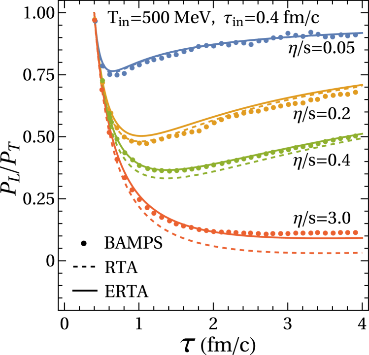
Figure 1: Evolution of $P_{L}/P_{T}$ in BAMPS (black dots) compared with hydrodynamic evolution using transport coefficients obtained from the RTA approximation (dashed curves) and ERTA approximation with $\ell=1/2$.

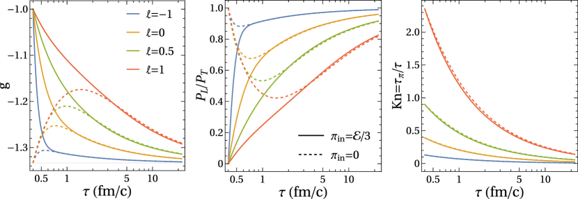
Figure 2: Time evolution of the quantity $g$, pressure anisotropy $P_{L}/P_{T}$, and Knudsen number $\tau_{\pi}/\tau$. Solid and dashed curves correspond to different initial shear stresses, $\pi={\cal E}/3,0$, respectively. The blue, orange, green, and red curves correspond to values of $\ell=-1,0,1/2,1$, respectively. As can be seen in all three panels, isotropization and thermalization are delayed as the value of $\ell$ is increased.

The hydrodynamic regime is reached when the scattering rate exceeds the expansion rate, i.e., $\tau_{\pi}\ll\tau$. The last term in the above equation is dominant in this regime, and the hydrodynamic fixed point $g_{*}$ is given by:

$$g_{*}=-\frac{4}{3}\,.$$ (43)

In the collisionless regime, the expansion rate far exceeds the scattering rate ($\tau_{\pi}\gg\tau$), and the function $\mathcal{B}(g)$ in Eq. (42) is dominated by the terms that do not depend on $\tau/\tau_{\pi}$. The zeros of this function correspond to the free-streaming fixed points,

$$g_{\rm fp}=-\left(\frac{8+\mathcal{C}}{6}\right)\pm\sqrt{\frac{4\beta_{\pi}}{3{\cal E}}+\frac{\mathcal{C}^{2}}{36}}\,,$$ (44)

with the positive root corresponding to the free-streaming stable fixed point. For a plasma undergoing Bjorken expansion, it has been shown that the stable free-streaming fixed point of the exact kinetic solution corresponds to vanishing longitudinal pressure, or $g=-1$ Chattopadhyay et al. (2022); Jaiswal et al. (2022a); Blaizot and Yan (2020). Using the parametrization (36) for the relaxation time and the corresponding values of the transport coefficients given in Eqs. (37) and (IV.3), we observe that the value of the stable fixed point in the exact kinetic equation ($g=-1$) can be recovered from Eq. (44) for $\ell\approx 0.763$. Extending the domain of Israel-Stewart-type hydrodynamic theories requires the hydrodynamic equations to accurately capture the location of the stable free-streaming fixed point, as emphasized in Ref. Jaiswal et al. (2022b). Therefore, the evolution Eq. (42), or analogously Eqs. (39) and (40), is expected to provide a good description of the underlying weakly coupled microscopic theory with $\ell\approx 0.763$, even in far-off-equilibrium regimes. It is worth mentioning that this value of $\ell$ is not arbitrary; many microscopic theories lie in the range $\ell=[0,1]$ Dusling et al. (2010).

To illustrate the impact of the ERTA framework, we show the comparison of the second-order hydrodynamic equations obtained from the RTA approximation ($\ell=0$) with those derived from the ERTA approximation setting $\ell=0.5$ and compare them with BAMPS results Xu and Greiner (2005); Xu et al. (2008); El et al. (2010) in Fig 1. The initial temperature is set to be $500\,$MeV at an initial time of $0.4\,$fm/c with a vanishing initial shear stress. Further, we fix the values of $\kappa$ appearing in Eqs. (37) and (IV.3) such that $\eta/s$ is set to different values as mentioned in the figure. As can be seen from the figure, the solid curves representing the ERTA approximation with $\ell=0.5$ are in an overall better agreement with the BAMPS solution than the dashed curves Mitra (2021).

In Figure 2, we present the evolution of three quantities: $g$, the pressure anisotropy $P_{L}/P_{T}=(P-\pi)/(P+\pi/2)$, and the Knudsen number $\tau_{\pi}/\tau$. The initial temperature is set to be $500\,$MeV at an initial time of $0.4\,$fm/c. Additionally, we consider the parameter $\kappa$ appearing in Eqs. (37) and (IV.3) to have the value $5/(4\pi)$. In all three panels, the solid curves represent cases where $P_{L}$ is initialized at $0$, corresponding to $\pi={\cal E}/3$, while the dashed curves are initialized with a vanishing initial shear stress, $\pi=0$. The blue, orange, green, and red curves correspond to different values of $\ell=-1,0,1/2,1$, respectively. The left panel displays the evolution of the quantity $g$, with the gray solid line representing the hydrodynamic fixed point $g_{*}$. It can be observed from the systematic trend of blue, orange, green, and red curves that the system remains out of equilibrium for a longer duration as the values of $\ell$ are increased. This feature is also visible in the middle panel where the evolution of pressure anisotropy, $P_{L}/P_{T}$ is shown – approach to $P_{L}/P_{T}=1$ is delayed for the orange, green, and red curves compared to the blue curve, indicating a slower isotropization. Also, in the left and middle panels we observe that the solid and dashed curves, representing different initial shear stress, overlap earlier for smaller values of $\ell$. Interestingly, the evolution of Knudsen number shown in the right panel is not strongly dependent on the initial values of shear stress but has a strong dependence on the strength of the momentum-dependence of the relaxation time i.e. on $\ell$; the solid and dashed curves largely overlap during the entire evolution. It is worth noting that increasing the value of $\ell$ enhances the initial gradient strength (as $\tau_{\pi}$ increases), and smaller values of $\ell$ drive the system towards thermalization at a faster rate, which is evident from the middle panel.

In Figure 3, we show the evolution of the temperature normalized with the ideal temperature evolution, $T_{\rm id}=T_{\rm in}(\tau_{\rm in}/\tau)^{1/3}$. It is observed that at a given time, the fluid maintains a higher temperature when the initial shear stress has a large positive value (solid curves), in contrast to when the initial shear stress is vanishing (dashed curves). An interesting observation is that increasing values of $\ell$ also lead to higher temperatures of the medium, as indicated by the trend of the differently colored curves. This may be understood from the right panel of Fig. 2, where we observe that an increase in the values of $\ell$ results in a larger Knudsen number. Consequently, this leads to increased dissipation, resulting in a slower fall of temperature compared to ideal evolution. Moreover, the interplay between the initial conditions for shear stress and the various medium interactions (characterized by different values of $\ell$) is intriguing, and can provide insights towards constraining the initial conditions for hydrodynamic simulation of heavy-ion collisions. Further, the various curves in Fig. 3 crossing the temperature surface of $155\,$MeV (represented by the black dotted curve) at different proper times suggests that a constant temperature particlization surface can be reached at different times with varying anisotropies. This can be seen more clearly in Fig. 4, where the evolution of the pressure anisotropy $P_{L}/P_{T}$ with $\tau/\tau_{\pi}$ is shown. The evolution of the curves is stopped when the temperature of the plasma reaches $155\,$MeV during the expansion (at times when the different curves cross the black dotted curve in Fig. 3). In Fig. 4, we see that the pressure anisotropy across the different colored curves differs significantly. We also note that the evolution of $P_{L}/P_{T}$ for different curves in the near-equilibrium regime ($\tau\gtrsim 5\tau_{\pi}$) is nearly the same, but differs substantially in the far-off-equilibrium regime.

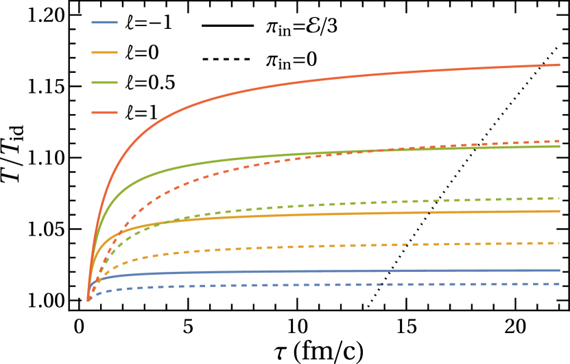
Figure 3: Time evolution of temperature normalized with ideal temperature evolution. The initial conditions and legends are the same as in Fig. 2. The black dotted curve represents a temperature surface of $155\,$MeV.

VI Summary and outlook

To summarize, we have derived relativistic second-order hydrodynamics from the Boltzmann equation using the extended relaxation time approximation for the collision kernel, incorporating an energy-dependent relaxation time. The transport coefficients are shown to explicitly depend on the microscopic relaxation rate. We investigated the fixed point structure of the hydrodynamic equations for a plasma undergoing Bjorken flow and showed that the location of the free-streaming fixed points depends on the energy dependence of the relaxation time. Additionally, we employed a power law parametrization to describe the energy dependence of the relaxation time and examined its impact on the thermalization process of the expanding plasma. We demonstrated that the plasma’s approach to equilibrium is affected by the relaxation time’s dependence on different powers of energy; the plasma remains in the out-off-equilibrium regime and at a higher temperature for longer duration as larger positive values of $\ell$ are considered.

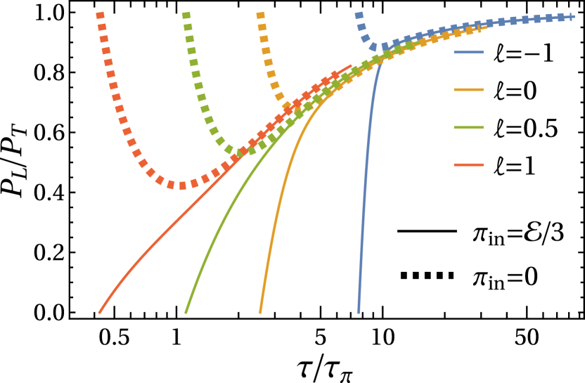
Figure 4: Evolution of pressure anisotropy $P_{L}/P_{T}$ with $\tau/\tau_{\pi}$. The evolution of different curves is stopped at proper times when the temperature evolution reaches $155\,$MeV.

While the derivation in the present article is done for a conformal system without conserved charges, it can be extended for non-conformal systems with conserved charges and quantum statistics by following the steps outlined in the article. It is also desired to have typical relaxation rates for the energy dependence of the relaxation time across different stages of the evolution of the nuclear matter formed in heavy-ion collisions. Such parametrization of the relaxation time can have parameters which may depend, for example, on the temperature of the medium. Incorporating these rates will make the full hydrodynamic equations with the associated transport coefficients more suitable for a (3+1)-dimensional hydrodynamic simulation. It should be noted that the functional form of the first-order transport coefficients, such as $\eta$, is determined within the framework. Furthermore, such an analysis may also provide insights into the form of distribution function at particlization. These aspects will be investigated in future studies.

Appendix A Derivation of $\delta u^{\mu}$ and $\delta T$

In this Appendix, we obtain $\delta u^{\mu}$ and $\delta T$ by imposing Landau frame and matching conditions. The Landau Frame condition, $u_{\mu}T^{\mu\nu}={\cal E}u^{\nu}$, with the matching ${\cal E}={\cal E}_{0}$, for a non-equilibrium distribution $f=f_{\rm eq}+\delta f$ can be written as

$$u_{\mu}\int\mathrm{dP}\,p^{\mu}p^{\nu}(f_{\rm eq}+\delta f)=u^{\nu}\int\mathrm{dP}\,(u\cdot p)^{2}f_{\rm eq}$$

$$\implies u_{\mu}\int\mathrm{dP}\,p^{\mu}p^{\nu}\delta f=u^{\nu}u_{\alpha}u_{\beta}I^{\alpha\beta}-u_{\mu}I^{\mu\nu}=0,$$ (45)

where $I^{\alpha\beta}=\int\mathrm{dP}\,p^{\alpha}p^{\beta}f_{\rm eq}$. Replacing $\delta f\mapsto\delta f_{(2)}$ obtained in Eq. (IV), and performing the integrals in the local rest frame of $u^{\mu}$, the above equation reduces to

$$I_{3,1}\delta u^{\mu}-I_{3,0}\frac{\delta T}{T}u^{\mu}+\frac{5K_{3,2}}{({\cal E}+{\cal P})}\left(\pi^{\mu\nu}\dot{u}_{\nu}-\nabla_{\nu}\pi^{\mu\nu}\right)$$

$$+\left(6L_{3,2}+2M_{4,2}-2\frac{N_{3,2}}{T}\right)\sigma^{\mu\nu}\dot{u}_{\nu}+2L_{3,2}\nabla_{\nu}\sigma^{\mu\nu}$$

$$+\left(10L_{3,2}-2\frac{L_{4,2}}{T}+2M_{4,2}\right)\sigma^{\alpha\beta}\sigma_{\alpha\beta}u^{\mu}=0.$$ (46)

Note that the term $\delta u\cdot u=(\delta u\cdot\delta u)/2\sim\mathcal{O}\left(\delta^{4}\right)$, since $\delta u^{\mu}$ is at least second order (see discussion in Section IV), and has been ignored in the derivation. Further, we have defined the thermodynamic integrals,

$$I_{n,q}\! \equiv\!\frac{1}{(2q+1)!!}\!\int\!\mathrm{dP}(u\cdot p)^{n-2q}(\Delta_{\alpha\beta}p^{\alpha}p^{\beta})^{q}\,f_{\rm eq},$$ (47)

$$M_{n,q}\! \equiv\!\frac{1}{(2q\!+\!1)!!}\!\int\!\!\mathrm{dP}\tau_{\rm R}\frac{\partial\tau_{\rm R}}{\partial(u\!\cdot\!p)}(u\!\cdot\!p)^{n-2q}(\Delta_{\alpha\beta}p^{\alpha}p^{\beta})^{q}f_{\rm eq},$$ (48)

$$N_{n,q}\! \equiv\!\frac{1}{(2q\!+\!1)!!}\!\int\!\mathrm{dP}\,\tau_{\rm R}\frac{\partial\tau_{\rm R}}{\partial\beta}(u\!\cdot\!p)^{n-2q}(\Delta_{\alpha\beta}p^{\alpha}p^{\beta})^{q}\,f_{\rm eq}.$$ (49)

We note that $M_{n,q}$ and $N_{n,q}$ integrals can be expressed in terms of the $L_{n,q}$ integrals through the relations,

$$M_{n,q} =\frac{1}{2T}L_{n,q}-\frac{n+1}{2}L_{n-1,q}\,,\quad\text{iff }n>-1\,,$$ (50)

$$2N_{n,q} =L_{n+1,q}-nTL_{n,q}\,.$$ (51)

Using these relations, Eq. (A) simplifies to,

$$I_{3,1}\delta u^{\mu}\!-I_{3,0}\frac{\delta T}{T}u^{\mu}\!+\frac{5K_{3,2}}{({\cal E}+{\cal P})}\left(\pi^{\mu\nu}\dot{u}_{\nu}\!-\nabla_{\nu}\pi^{\mu\nu}\right)\!+2L_{3,2}$$

$$\times\!\left(2\sigma^{\mu\nu}\dot{u}_{\nu}\!+\!\nabla_{\nu}\sigma^{\mu\nu}\right)+\!\left(\!5L_{3,2}\!-\!\frac{L_{4,2}}{T}\!\right)\!\sigma^{\alpha\beta}\sigma_{\alpha\beta}u^{\mu}=0.$$ (52)

Similarly, using the matching condition:

$$u_{\mu}u_{\nu}T^{\mu\nu}={\cal E}_{0}\implies u_{\mu}u_{\nu}\int\mathrm{dP}\,p^{\mu}p^{\nu}\delta f=0\,,$$ (53)

and replacing $\delta f\mapsto\delta f_{(2)}$ obtained in Eq. (IV), we obtain

$$-I_{3,0}\frac{\delta T}{T}+\frac{5K_{3,2}}{{\cal E}\!+\!{\cal P}}\pi^{\mu\nu}\sigma_{\mu\nu}+\!\left(\!3L_{3,2}-\frac{L_{4,2}}{T}\!\right)\!\sigma^{\mu\nu}\sigma_{\mu\nu}=0\,.$$ (54)

Noting that $I_{3,0}=3T({\cal E}\!+\!{\cal P})$ and solving for $\delta T$, we obtain

$$\delta T=\frac{5}{3}\frac{K_{3,2}}{({\cal E}\!+\!{\cal P})^{2}}\pi^{\mu\nu}\sigma_{\mu\nu}+\frac{1}{{\cal E}\!+\!{\cal P}}\!\left(\!L_{3,2}-\frac{L_{4,2}}{3T}\!\right)\!\sigma^{\mu\nu}\sigma_{\mu\nu}\,.$$ (55)

The expression for $\delta u^{\nu}$ is obtained by using Eq. (54) in Eq. (A),

$$\delta u^{\mu} =\frac{5K_{3,2}}{T({\cal E}\!+\!{\cal P})^{2}}\left(\pi^{\mu\nu}\dot{u}_{\nu}-\nabla_{\nu}\pi^{\mu\nu}-\pi^{\alpha\beta}\sigma_{\alpha\beta}u^{\mu}\right)$$

$$+\frac{2L_{3,2}}{T({\cal E}\!+\!{\cal P})}\left(2\sigma^{\mu\nu}\dot{u}_{\nu}+\nabla_{\nu}\sigma^{\mu\nu}+\sigma^{\alpha\beta}\sigma_{\alpha\beta}u^{\mu}\right),$$ (56)

where we have used the relation $I_{3,1}=-T({\cal E}\!+\!{\cal P})$.

In the case when the relaxation time is independent of the particle energies, the integrals $K_{n,q}\to\tau_{\rm R}\,I_{n,q}$ and $L_{n,q}\to\tau_{\rm R}^{2}\,I_{n,q}=\tau_{\rm R}K_{n,q}$. Using these, and noting that $\tau_{\rm R}=5\eta/({\cal E}\!+\!{\cal P})$, Eq. (A) simplifies to

$$\delta u^{\mu} =\frac{5K_{3,2}}{T({\cal E}\!+\!{\cal P})^{2}}\left(\pi^{\mu\nu}\dot{u}_{\nu}-\nabla_{\nu}\pi^{\mu\nu}-\pi^{\alpha\beta}\sigma_{\alpha\beta}u^{\mu}\right)$$

$$+\frac{5K_{3,2}}{T({\cal E}\!+\!{\cal P})^{2}}2\eta\left(2\sigma^{\mu\nu}\dot{u}_{\nu}+\nabla_{\nu}\sigma^{\mu\nu}+\sigma^{\alpha\beta}\sigma_{\alpha\beta}u^{\mu}\right)$$

$$=\frac{5K_{3,2}}{T({\cal E}\!+\!{\cal P})^{2}}\left(3\pi^{\mu\nu}\dot{u}_{\nu}-\nabla_{\nu}\pi^{\mu\nu}+2\eta\nabla_{\nu}\sigma^{\mu\nu}\right)$$

$$=0\,.$$ (57)

In transitioning to the second equality, we employed the first-order relation $\pi^{\mu\nu}=2\eta\sigma^{\mu\nu}$. Furthermore, we used the relation $\nabla_{\nu}\eta=-3T\eta\nabla_{\nu}\beta=3\eta\dot{u}_{\nu}$ in the last equality.

Similarly, Eq. (55) reduces to

$$\delta T =\frac{1}{{\cal E}\!+\!{\cal P}}\!\left[\frac{5}{3}\frac{K_{3,2}}{({\cal E}\!+\!{\cal P})}\pi^{\mu\nu}\!\sigma_{\mu\nu}\!+\tau_{\rm R}^{2}\!\left(\!\!I_{3,2}\!-\!\frac{5}{3}I_{3,2}\!\!\right)\!\sigma^{\mu\nu}\!\sigma_{\mu\nu}\!\right]$$

$$=\frac{1}{{\cal E}\!+\!{\cal P}}\!\left[\frac{5}{3}\frac{K_{3,2}}{({\cal E}\!+\!{\cal P})}\pi^{\mu\nu}\sigma_{\mu\nu}-\frac{5\eta}{({\cal E}\!+\!{\cal P})}\frac{2}{3}K_{3,2}\sigma^{\mu\nu}\sigma_{\mu\nu}\right]$$

$$=0\,.$$ (58)

The fact that $\delta u^{\mu}$ and $\delta T$ vanish when the relaxation time is independent of particle energy is anticipated since ERTA reduces to the Anderson-Witting RTA, thus providing a consistency validation.

Appendix B Microscopic conservation at third order

In this appendix, we demonstrate microscopic energy-momentum conservation up to third order. The non-equilibrium correction to the equilibrium distribution function up to third order in spacetime gradients from the Boltzmann equation is obtained to be,

$$\Delta f_{(3)}= \Delta f^{*}_{(3)}-\frac{\tau_{\rm R}}{(u\cdot p)}p^{\mu}\partial_{\mu}\left[f_{\rm eq}-\frac{\tau_{\rm R}}{(u\cdot p)}p^{\rho}\partial_{\rho}f_{\rm eq}\right.$$

$$+\frac{\tau_{\rm R}}{(u\cdot p)}p^{\rho}p^{\nu}\partial_{\rho}\left(\frac{\tau_{\rm R}}{(u\cdot p)}\partial_{\nu}f_{\rm eq}\right)$$

$$\left.-\frac{\tau_{\rm R}}{(u\cdot p)}p^{\rho}\partial_{\rho}\Delta f^{*}_{(1)}+\Delta f^{*}_{(2)}\right].$$ (59)

As discussed in Sec. IV.2, verifying microscopic energy-momentum conservation up to the third order amounts to showing that the first momentum-moment of the collision kernel vanishes. Substituting $f\mapsto f_{(3)}=f_{\rm eq}+\Delta f_{(3)}$, and using Eq. (59),

$$\int\mathrm{dP}\,p^{\nu}\mathfrak{C}[f]=-\int\mathrm{dP}\,\frac{(u\cdot p)}{\tau_{\rm R}}p^{\nu}\left(\Delta f_{(3)}-\Delta f^{*}_{(3)}\right)$$

$$=\underbrace{\int\!\mathrm{dP}\,p^{\nu}p^{\mu}\left(\partial_{\mu}f_{\rm eq}\right)}_{I}+\underbrace{\int\!\mathrm{dP}\,p^{\nu}p^{\mu}p^{\rho}\partial_{\mu}\left[-\frac{\tau_{\rm R}}{(u\cdot p)}\left(\partial_{\rho}f_{\rm eq}\right)\right]}_{II}$$

$$+\underbrace{\int\!\mathrm{dP}\,p^{\nu}p^{\mu}p^{\rho}p^{\lambda}\partial_{\mu}\left[\frac{\tau_{\rm R}}{(u\cdot p)}\partial_{\rho}\left\{\frac{\tau_{\rm R}}{(u\cdot p)}\left(\partial_{\lambda}f_{\rm eq}\right)\right\}\right]}_{III}$$

$$+\underbrace{\int\!\mathrm{dP}\,p^{\nu}p^{\mu}p^{\rho}\partial_{\mu}\!\left[\frac{\tau_{\rm R}}{(u\cdot p)}\!\left(\!\partial_{\rho}\Delta f^{*}_{(1)}\!\right)\!\right]}_{IV}\!+\!\underbrace{\int\!\mathrm{dP}\,p^{\nu}p^{\mu}\!\left(\!\partial_{\mu}\Delta f^{*}_{(2)}\!\right)\!}_{V}.$$ (60)

Evaluating these integrals, we find,

$$\textit{I}= \dot{u}_{\mu}\pi^{\mu\nu}-\nabla_{\mu}\pi^{\mu\nu}=-\partial_{\mu}\pi^{\mu\nu}\,,$$ (61)

$$\textit{II}= \partial_{\mu}\!\bigg{[}\!\frac{2K_{3,2}}{T}\sigma^{\mu\nu}+\frac{5K_{3,2}}{T({\cal E}+{\cal P})}\!\bigg{\{}\!\!\left(\!u^{\mu}u^{\nu}\!+\!\frac{\Delta^{\mu\nu}}{3}\!\right)\!\pi^{\alpha\beta}\sigma_{\alpha\beta}$$

$$\quad\!+\!u^{\mu}\nabla_{\gamma}\pi^{\nu\gamma}+u^{\nu}\nabla_{\gamma}\pi^{\mu\gamma}\!-\!\dot{u}_{\gamma}\left(u^{\mu}\pi^{\nu\gamma}+u^{\nu}\pi^{\mu\gamma}\right)\!\Big{\}}\!\bigg{]}.$$ (62)

In deriving, we have used the hydrodynamic evolution equations (7) and (8). The integral III, consistently keeping all terms till third order in gradients, is obtained to be,

$$\textit{III}= \partial_{\mu}\!\left[-\frac{2L_{3,2}}{T}\Big{\{}\dot{\sigma}^{\mu\nu}\!+\!\frac{1}{3}\sigma^{\mu\nu}\theta+u^{\mu}\nabla_{\rho}\sigma^{\nu\rho}+u^{\nu}\nabla_{\rho}\sigma^{\mu\rho}\right.$$

$$\qquad+3\dot{u}_{\rho}\left(u^{\mu}\sigma^{\nu\rho}+u^{\nu}\sigma^{\mu\rho}\right)+\omega^{\nu}_{\rho}\sigma^{\mu\rho}+\omega^{\mu}_{\rho}\sigma^{\nu\rho}\!\Big{\}}$$

$$\qquad+\left(\frac{L_{3,2}}{T}-\frac{1}{7}\frac{L_{4,2}}{T^{2}}\right)\left(\Delta^{\mu\nu}-7u^{\mu}u^{\nu}\right)\sigma_{\alpha\beta}\sigma^{\alpha\beta}$$

$$\qquad\left.-\,\frac{4}{7}\frac{L_{4,2}}{T^{2}}\sigma^{\mu}_{\rho}\sigma^{\nu\rho}\right]+\order{\partial^{4}}\,.$$ (63)

The above equation can be further simplified by using the second-order constitutive relation (IV.3) for the shear stress tensor which can be written as,

$$\pi^{\mu\nu} =\frac{2K_{3,2}}{T}\sigma^{\mu\nu}+\frac{4}{7}\frac{L_{4,2}}{T^{2}}\left(\frac{1}{3}\Delta^{\mu\nu}\sigma_{\alpha\beta}\sigma^{\alpha\beta}-\sigma^{\mu}_{\rho}\sigma^{\nu\rho}\right)$$

$$\!-\!\frac{2L_{3,2}}{T}\!\left(\!\dot{\sigma}^{\mu\nu}\!+\!\frac{1}{3}\sigma^{\mu\nu}\theta\!+\!\omega^{\nu}_{\rho}\sigma^{\mu\rho}\!+\!\omega^{\mu}_{\rho}\sigma^{\nu\rho}\!+\!\dot{u}_{\rho}(u^{\mu}\sigma^{\nu\rho}\!+\!u^{\nu}\sigma^{\mu\rho})\!\right)\!.$$ (64)

Replacing the $\dot{\sigma}^{\mu\nu}$ term in Eq. (63) using the above equation, integral III simplifies to,

III $$=\partial_{\mu}\left[\pi^{\mu\nu}-\frac{2K_{3,2}}{T}\sigma^{\mu\nu}+\frac{L_{4,2}}{T^{2}}\left(u^{\mu}u^{\nu}-\frac{\Delta^{\mu\nu}}{3}\right)\sigma^{\alpha\beta}\sigma_{\alpha\beta}\right.$$

$$\qquad\quad\!-\!\frac{2L_{3,2}}{T}\!\bigg{\{}\!u^{\mu}\nabla_{\rho}\sigma^{\nu\rho}\!+\!u^{\nu}\nabla_{\rho}\sigma^{\mu\rho}\!+\!2\dot{u}_{\rho}(u^{\mu}\sigma^{\nu\rho}+u^{\nu}\sigma^{\mu\rho})$$

$$\qquad\qquad\qquad\quad\left.+\frac{1}{2}\left(7u^{\mu}u^{\nu}-\Delta^{\mu\nu}\right)\sigma^{\alpha\beta}\sigma_{\alpha\beta}\bigg{\}}\right]+\order{\partial^{4}}\,.$$ (65)

Note that the replacement using Eq. (IV.3) (or Eq. (64)) keeps the integral III exact up to third order.

Adding the contributions of the integrals I, II and III using Eqs. (61, 62, 65):

$$\textit{I}+\textit{II}+\textit{III}=\partial_{\mu}\bigg{[} \frac{5K_{3,2}}{T({\cal E}+{\cal P})}\left\{\!\left(\!u^{\mu}u^{\nu}+\frac{\Delta^{\mu\nu}}{3}\!\right)\!\pi^{\alpha\beta}\sigma_{\alpha\beta}+u^{\mu}\nabla_{\rho}\pi^{\nu\rho}+u^{\nu}\nabla_{\rho}\pi^{\mu\rho}-\dot{u}_{\rho}\left(u^{\mu}\pi^{\nu\rho}+u^{\nu}\pi^{\mu\rho}\right)\right\}$$

$$-\frac{2L_{3,2}}{T}\left\{u^{\mu}\nabla_{\rho}\sigma^{\nu\rho}+u^{\nu}\nabla_{\rho}\sigma^{\mu\rho}+2\dot{u}_{\rho}(u^{\mu}\sigma^{\nu\rho}+u^{\nu}\sigma^{\mu\rho})+\frac{1}{2}\left(7u^{\mu}u^{\nu}-\Delta^{\mu\nu}\right)\sigma^{\alpha\beta}\sigma_{\alpha\beta}\right\}$$

$$+\frac{L_{4,2}}{T^{2}}\left(u^{\mu}u^{\nu}-\frac{\Delta^{\mu\nu}}{3}\right)\sigma^{\alpha\beta}\sigma_{\alpha\beta}\bigg{]}+\order{\partial^{4}}\,.$$ (66)

It can be verified that the above combination vanishes when the relaxation time is independent of particle momenta. This is consistent with third-order hydrodynamics derived using the RTA approximation of the collision kernel Jaiswal (2013b).

We now evaluate the two integrals, IV and V, which are due to the difference between the ‘thermodynamic’ and hydrodynamic frames. Since $\Delta f^{*}_{(1)}$ contains the terms $\delta u^{\mu},\,\delta T$ which are at least $\order{\partial^{2}}$, the integral IV,

$$\textit{IV}=\!\int\!\mathrm{dP}p^{\nu}p^{\mu}p^{\rho}\partial_{\mu}\left[\frac{\tau_{\rm R}}{(u\cdot p)}\left(\partial_{\rho}\Delta f^{*}_{(1)}\right)\right]=\order{\partial^{4}}$$ (67)

is at least $\order{\partial^{4}}$ and can be ignored. The remaining integral V simplifies to

V $$=\int\mathrm{dP}\,p^{\nu}p^{\mu}\left(\partial_{\mu}\Delta f^{*}_{(2)}\right)$$

$$=\partial_{\mu}\!\left[\!-\frac{I_{3,1}}{T}\left(u^{\nu}\delta u^{\mu}+u^{\mu}\delta u^{\nu}\right)\!+\!\frac{\delta T}{T^{2}}\left(u^{\mu}u^{\nu}I_{3,0}+\Delta^{\mu\nu}I_{3,1}\right)\!\right]\!$$

$$=\partial_{\mu}\!\left[\!({\cal E}+{\cal P})\!\left\{\!\left(u^{\nu}\delta u^{\mu}+u^{\mu}\delta u^{\nu}\right)\!+\!\frac{\delta T}{T}\left(3u^{\mu}u^{\nu}\!-\!\Delta^{\mu\nu}\right)\!\right\}\!\right]\!,$$ (68)

where we have not considered the terms $\left(u\cdot\delta u\right)=-(\delta u)^{2}/2,\,(\delta u)^{2},\,(\delta T)^{2},\,\delta u^{\mu}\delta T$, and higher order terms in the Taylor expansion of $\Delta f^{*}_{(2)}$ as they are at least $\order{\partial^{4}}$. Hence, the expansion of $\Delta f^{*}_{(2)}$ only involves contributions from the terms $\delta u^{\mu}$ and $\delta T$, and their determination imposing Landau frame and matching conditions remains identical as done for second-order in Appendix A. The relevant expressions for $\delta u^{\mu}$ and $\delta T$ can be found in Eqs. (IV.1) and (26). It is important to note that when the relaxation time is independent of particle energies, both $\delta u^{\mu}$ and $\delta T$ vanish, as demonstrated in Appendix A, resulting in the integral V also vanishing.

Using these, the integral (68) can be written as,

$$\textit{V}= \partial_{\mu}\left[\frac{u^{\nu}}{T}\left\{\frac{5K_{3,2}}{({\cal E}+{\cal P})}\left(\pi^{\mu\rho}\dot{u}_{\rho}-\nabla_{\rho}\pi^{\mu\rho}-\pi^{\alpha\beta}\sigma_{\alpha\beta}u^{\mu}\right)+2L_{3,2}\left(2\sigma^{\mu\rho}\dot{u}_{\rho}+\nabla_{\rho}\sigma^{\mu\rho}+\sigma^{\alpha\beta}\sigma_{\alpha\beta}u^{\mu}\right)\right\}\right.$$

$$\qquad\quad+\frac{u^{\mu}}{T}\left\{\frac{5K_{3,2}}{({\cal E}\!+\!{\cal P})}\left(\pi^{\nu\rho}\dot{u}_{\rho}-\nabla_{\rho}\pi^{\nu\rho}-\pi^{\alpha\beta}\sigma_{\alpha\beta}u^{\nu}\right)+2L_{3,2}\left(2\sigma^{\nu\rho}\dot{u}_{\rho}+\nabla_{\rho}\sigma^{\nu\rho}+\sigma^{\alpha\beta}\sigma_{\alpha\beta}u^{\nu}\right)\right\}$$

$$\qquad\quad\left.+\frac{1}{T}\left\{\frac{5}{3}\frac{K_{3,2}}{({\cal E}+{\cal P})}\pi^{\alpha\beta}\sigma_{\alpha\beta}+\left(L_{3,2}-\frac{L_{4,2}}{3T}\right)\sigma^{\alpha\beta}\sigma_{\alpha\beta}\right\}\left(3u^{\mu}u^{\nu}\!-\!\Delta^{\mu\nu}\right)\right]+\order{\partial^{4}}\,,$$

$$= -\partial_{\mu}\bigg{[}\frac{5K_{3,2}}{T({\cal E}+{\cal P})}\left\{\!\left(\!u^{\mu}u^{\nu}+\frac{\Delta^{\mu\nu}}{3}\!\right)\!\pi^{\alpha\beta}\sigma_{\alpha\beta}+u^{\mu}\nabla_{\rho}\pi^{\nu\rho}+u^{\nu}\nabla_{\rho}\pi^{\mu\rho}-\dot{u}_{\rho}\left(u^{\mu}\pi^{\nu\rho}+u^{\nu}\pi^{\mu\rho}\right)\right\}$$

$$\qquad\quad-\frac{2L_{3,2}}{T}\left\{u^{\mu}\nabla_{\rho}\sigma^{\nu\rho}+u^{\nu}\nabla_{\rho}\sigma^{\mu\rho}+2\dot{u}_{\rho}(u^{\mu}\sigma^{\nu\rho}+u^{\nu}\sigma^{\mu\rho})+\frac{1}{2}\left(7u^{\mu}u^{\nu}-\Delta^{\mu\nu}\right)\sigma^{\alpha\beta}\sigma_{\alpha\beta}\right\}$$

$$\qquad\quad+\frac{L_{4,2}}{T^{2}}\left(u^{\mu}u^{\nu}-\frac{\Delta^{\mu\nu}}{3}\right)\sigma^{\alpha\beta}\sigma_{\alpha\beta}\bigg{]}+\order{\partial^{4}}\,.$$ (69)

This above expression precisely cancels the terms in Eq. (66) up to $\order{\partial^{3}}$, i.e.,

$$\int\mathrm{dP}\,p^{\nu}\mathfrak{C}[f]=(\textit{I}+\textit{II}+\textit{III})+\textit{IV}+\textit{V}=\order{\partial^{4}}\,,$$ (70)

therefore ensuring the energy-momentum conservation up to third order.

References

- Muronga (2007) Azwinndini Muronga, “Relativistic Dynamics of Non-ideal Fluids: Viscous and heat-conducting fluids. II. Transport properties and microscopic description of relativistic nuclear matter,” Phys. Rev. C 76, 014910 (2007), arXiv:nucl-th/0611091 .
- York and Moore (2009) Mark Abraao York and Guy D. Moore, “Second order hydrodynamic coefficients from kinetic theory,” Phys. Rev. D 79, 054011 (2009), arXiv:0811.0729 [hep-ph] .
- Betz et al. (2009) B. Betz, D. Henkel, and D. H. Rischke, “From kinetic theory to dissipative fluid dynamics,” Prog. Part. Nucl. Phys. 62, 556–561 (2009), arXiv:0812.1440 [nucl-th] .
- Romatschke (2010) Paul Romatschke, “New Developments in Relativistic Viscous Hydrodynamics,” Int. J. Mod. Phys. E 19, 1–53 (2010), arXiv:0902.3663 [hep-ph] .
- Denicol et al. (2012) G. S. Denicol, H. Niemi, E. Molnar, and D. H. Rischke, “Derivation of transient relativistic fluid dynamics from the Boltzmann equation,” Phys. Rev. D 85, 114047 (2012), [Erratum: Phys.Rev.D 91, 039902 (2015)], arXiv:1202.4551 [nucl-th] .
- Florkowski et al. (2013) Wojciech Florkowski, Radoslaw Ryblewski, and Michael Strickland, “Testing viscous and anisotropic hydrodynamics in an exactly solvable case,” Phys. Rev. C 88, 024903 (2013), arXiv:1305.7234 [nucl-th] .
- Weickgenannt et al. (2021) Nora Weickgenannt, Enrico Speranza, Xin-li Sheng, Qun Wang, and Dirk H. Rischke, “Generating Spin Polarization from Vorticity through Nonlocal Collisions,” Phys. Rev. Lett. 127, 052301 (2021), arXiv:2005.01506 [hep-ph] .
- Bhatnagar et al. (1954) P.L. Bhatnagar, E.P. Gross, and M. Krook, “A Model for Collision Processes in Gases. 1. Small Amplitude Processes in Charged and Neutral One-Component Systems,” Phys. Rev. 94, 511–525 (1954).
- Welander (1954) P Welander, “On the temperature jump in a rarefied gas,” Arkiv Fysik 7, 507 (1954).
- Marle (1969) Charles M. Marle, “Sur l’établissement des équations de l’hydrodynamique des fluides relativistes dissipatifs. I. - L’équation de Boltzmann relativiste,” Ann. Phys. Theor. 10, 67–126 (1969).
- Anderson and Witting (1974) James L Anderson and HR Witting, “A relativistic relaxation-time model for the boltzmann equation,” Physica 74, 466–488 (1974).
- Denicol et al. (2010) G. S. Denicol, T. Koide, and D. H. Rischke, “Dissipative relativistic fluid dynamics: a new way to derive the equations of motion from kinetic theory,” Phys. Rev. Lett. 105, 162501 (2010), arXiv:1004.5013 [nucl-th] .
- Jaiswal (2013a) Amaresh Jaiswal, “Relativistic dissipative hydrodynamics from kinetic theory with relaxation time approximation,” Phys. Rev. C 87, 051901 (2013a), arXiv:1302.6311 [nucl-th] .
- Jaiswal et al. (2014) Amaresh Jaiswal, Radoslaw Ryblewski, and Michael Strickland, “Transport coefficients for bulk viscous evolution in the relaxation time approximation,” Phys. Rev. C 90, 044908 (2014), arXiv:1407.7231 [hep-ph] .
- Mohanty et al. (2019) Payal Mohanty, Ashutosh Dash, and Victor Roy, “One particle distribution function and shear viscosity in magnetic field: a relaxation time approach,” Eur. Phys. J. A 55, 35 (2019), arXiv:1804.01788 [nucl-th] .
- Kurian (2020) Manu Kurian, “Thermal transport in a weakly magnetized hot QCD medium,” Phys. Rev. D 102, 014041 (2020), arXiv:2005.04247 [nucl-th] .
- Gabbana et al. (2017) A. Gabbana, M. Mendoza, S. Succi, and R. Tripiccione, “Kinetic approach to relativistic dissipation,” Phys. Rev. E 96, 023305 (2017), arXiv:1704.02523 [physics.comp-ph] .
- Bhadury et al. (2020) Samapan Bhadury, Wojciech Florkowski, Amaresh Jaiswal, and Radoslaw Ryblewski, “Relaxation time approximation with pair production and annihilation processes,” Phys. Rev. C 102, 064910 (2020), arXiv:2006.14252 [hep-ph] .
- Panda et al. (2021) Ankit Kumar Panda, Ashutosh Dash, Rajesh Biswas, and Victor Roy, “Relativistic non-resistive viscous magnetohydrodynamics from the kinetic theory: a relaxation time approach,” JHEP 03, 216 (2021), arXiv:2011.01606 [nucl-th] .
- Vyas et al. (2023) Nisarg Vyas, Sunil Jaiswal, and Amaresh Jaiswal, “Metric anisotropies and nonequilibrium attractor for expanding plasma,” Phys. Lett. B 841, 137943 (2023), arXiv:2212.02451 [nucl-th] .
- Singha et al. (2023) Pracheta Singha, Samapan Bhadury, Arghya Mukherjee, and Amaresh Jaiswal, “Relativistic BGK hydrodynamics,” (2023), arXiv:2301.00544 [nucl-th] .
- Heller et al. (2018) Michal P. Heller, Aleksi Kurkela, Michal Spaliński, and Viktor Svensson, “Hydrodynamization in kinetic theory: Transient modes and the gradient expansion,” Phys. Rev. D 97, 091503 (2018), arXiv:1609.04803 [nucl-th] .
- Blaizot and Yan (2018) Jean-Paul Blaizot and Li Yan, “Fluid dynamics of out of equilibrium boost invariant plasmas,” Phys. Lett. B 780, 283–286 (2018), arXiv:1712.03856 [nucl-th] .
- Florkowski et al. (2018) Wojciech Florkowski, Michal P. Heller, and Michal Spalinski, “New theories of relativistic hydrodynamics in the LHC era,” Rept. Prog. Phys. 81, 046001 (2018), arXiv:1707.02282 [hep-ph] .
- Strickland (2018) M. Strickland, “The non-equilibrium attractor for kinetic theory in relaxation time approximation,” JHEP 12, 128 (2018), arXiv:1809.01200 [nucl-th] .
- Chattopadhyay et al. (2018) Chandrodoy Chattopadhyay, Ulrich Heinz, Subrata Pal, and Gojko Vujanovic, “Higher order and anisotropic hydrodynamics for Bjorken and Gubser flows,” Phys. Rev. C 97, 064909 (2018), arXiv:1801.07755 [nucl-th] .
- Kurkela et al. (2020) Aleksi Kurkela, Wilke van der Schee, Urs Achim Wiedemann, and Bin Wu, “Early- and Late-Time Behavior of Attractors in Heavy-Ion Collisions,” Phys. Rev. Lett. 124, 102301 (2020), arXiv:1907.08101 [hep-ph] .
- Blaizot and Yan (2020) Jean-Paul Blaizot and Li Yan, “Emergence of hydrodynamical behavior in expanding ultra-relativistic plasmas,” Annals Phys. 412, 167993 (2020), arXiv:1904.08677 [nucl-th] .
- Blaizot and Yan (2021a) Jean-Paul Blaizot and Li Yan, “Analytical attractor for Bjorken flows,” Phys. Lett. B 820, 136478 (2021a), arXiv:2006.08815 [nucl-th] .
- Dash and Roy (2020) Ashutosh Dash and Victor Roy, “Hydrodynamic attractors for Gubser flow,” Phys. Lett. B 806, 135481 (2020), arXiv:2001.10756 [nucl-th] .
- Jaiswal et al. (2021) Amaresh Jaiswal et al., “Dynamics of QCD matter — current status,” Int. J. Mod. Phys. E 30, 2130001 (2021), arXiv:2007.14959 [hep-ph] .
- Soloviev (2022) Alexander Soloviev, “Hydrodynamic attractors in heavy ion collisions: a review,” Eur. Phys. J. C 82, 319 (2022), arXiv:2109.15081 [hep-th] .
- Blaizot and Yan (2021b) Jean-Paul Blaizot and Li Yan, “Attractor and fixed points in Bjorken flows,” Phys. Rev. C 104, 055201 (2021b), arXiv:2106.10508 [nucl-th] .
- Chattopadhyay et al. (2022) Chandrodoy Chattopadhyay, Sunil Jaiswal, Lipei Du, Ulrich Heinz, and Subrata Pal, “Non-conformal attractor in boost-invariant plasmas,” Phys. Lett. B 824, 136820 (2022), arXiv:2107.05500 [nucl-th] .
- Jaiswal et al. (2022a) Sunil Jaiswal, Chandrodoy Chattopadhyay, Lipei Du, Ulrich Heinz, and Subrata Pal, “Nonconformal kinetic theory and hydrodynamics for Bjorken flow,” Phys. Rev. C 105, 024911 (2022a), arXiv:2107.10248 [hep-ph] .
- Jaiswal et al. (2022b) Sunil Jaiswal, Jean-Paul Blaizot, Rajeev S. Bhalerao, Zenan Chen, Amaresh Jaiswal, and Li Yan, “From moments of the distribution function to hydrodynamics: The nonconformal case,” Phys. Rev. C 106, 044912 (2022b), arXiv:2208.02750 [nucl-th] .
- Chattopadhyay et al. (2023) Chandrodoy Chattopadhyay, Ulrich Heinz, and Thomas Schaefer, “Far-off-equilibrium expansion trajectories in the QCD phase diagram,” Phys. Rev. C 107, 044905 (2023), arXiv:2209.10483 [hep-ph] .
- Ambrus et al. (2023) Victor E. Ambrus, S. Schlichting, and C. Werthmann, “Establishing the Range of Applicability of Hydrodynamics in High-Energy Collisions,” Phys. Rev. Lett. 130, 152301 (2023), arXiv:2211.14356 [hep-ph] .
- Jankowski and Spaliński (2023) Jakub Jankowski and Michał Spaliński, “Hydrodynamic attractors in ultrarelativistic nuclear collisions,” Prog. Part. Nucl. Phys. 132, 104048 (2023), arXiv:2303.09414 [nucl-th] .
- Dusling et al. (2010) Kevin Dusling, Guy D. Moore, and Derek Teaney, “Radiative energy loss and v(2) spectra for viscous hydrodynamics,” Phys. Rev. C 81, 034907 (2010), arXiv:0909.0754 [nucl-th] .
- Chakraborty and Kapusta (2011) P. Chakraborty and J.I. Kapusta, “Quasi-Particle Theory of Shear and Bulk Viscosities of Hadronic Matter,” Phys. Rev. C 83, 014906 (2011), arXiv:1006.0257 [nucl-th] .
- Dusling and Schäfer (2012) Kevin Dusling and Thomas Schäfer, “Bulk viscosity, particle spectra and flow in heavy-ion collisions,” Phys. Rev. C 85, 044909 (2012), arXiv:1109.5181 [hep-ph] .
- Kurkela and Wiedemann (2019) Aleksi Kurkela and Urs Achim Wiedemann, “Analytic structure of nonhydrodynamic modes in kinetic theory,” Eur. Phys. J. C 79, 776 (2019), arXiv:1712.04376 [hep-ph] .
- Teaney and Yan (2014) Derek Teaney and Li Yan, “Second order viscous corrections to the harmonic spectrum in heavy ion collisions,” Phys. Rev. C 89, 014901 (2014), arXiv:1304.3753 [nucl-th] .
- Mitra (2021) Sukanya Mitra, “Relativistic hydrodynamics with momentum dependent relaxation time,” Phys. Rev. C 103, 014905 (2021), arXiv:2009.06320 [nucl-th] .
- Rocha et al. (2021) Gabriel S. Rocha, Gabriel S. Denicol, and Jorge Noronha, “Novel Relaxation Time Approximation to the Relativistic Boltzmann Equation,” Phys. Rev. Lett. 127, 042301 (2021), arXiv:2103.07489 [nucl-th] .
- Dash et al. (2022) Dipika Dash, Samapan Bhadury, Sunil Jaiswal, and Amaresh Jaiswal, “Extended relaxation time approximation and relativistic dissipative hydrodynamics,” Phys. Lett. B 831, 137202 (2022), arXiv:2112.14581 [nucl-th] .
- Gale et al. (2013) Charles Gale, Sangyong Jeon, and Bjoern Schenke, “Hydrodynamic Modeling of Heavy-Ion Collisions,” Int. J. Mod. Phys. A 28, 1340011 (2013), arXiv:1301.5893 [nucl-th] .
- Derradi de Souza et al. (2016) R. Derradi de Souza, Tomoi Koide, and Takeshi Kodama, “Hydrodynamic Approaches in Relativistic Heavy Ion Reactions,” Prog. Part. Nucl. Phys. 86, 35–85 (2016), arXiv:1506.03863 [nucl-th] .
- Schenke et al. (2020) Bjoern Schenke, Chun Shen, and Prithwish Tribedy, “Running the gamut of high energy nuclear collisions,” Phys. Rev. C 102, 044905 (2020), arXiv:2005.14682 [nucl-th] .
- Heinz and Snellings (2013) Ulrich Heinz and Raimond Snellings, “Collective flow and viscosity in relativistic heavy-ion collisions,” Ann. Rev. Nucl. Part. Sci. 63, 123–151 (2013), arXiv:1301.2826 [nucl-th] .
- Romatschke and Romatschke (2007) Paul Romatschke and Ulrike Romatschke, “Viscosity Information from Relativistic Nuclear Collisions: How Perfect is the Fluid Observed at RHIC?” Phys. Rev. Lett. 99, 172301 (2007), arXiv:0706.1522 [nucl-th] .
- Song and Heinz (2008) Huichao Song and Ulrich W. Heinz, “Suppression of elliptic flow in a minimally viscous quark-gluon plasma,” Phys. Lett. B 658, 279–283 (2008), arXiv:0709.0742 [nucl-th] .
- Buchel and Pagnutti (2009) Alex Buchel and Chris Pagnutti, “Bulk viscosity of N=2* plasma,” Nucl. Phys. B 816, 62–72 (2009), arXiv:0812.3623 [hep-th] .
- Denicol et al. (2009) G. S. Denicol, T. Kodama, T. Koide, and Ph. Mota, “Effect of bulk viscosity on Elliptic Flow near QCD phase transition,” Phys. Rev. C 80, 064901 (2009), arXiv:0903.3595 [hep-ph] .
- Ryu et al. (2015) S. Ryu, J. F. Paquet, C. Shen, G. S. Denicol, B. Schenke, S. Jeon, and C. Gale, “Importance of the Bulk Viscosity of QCD in Ultrarelativistic Heavy-Ion Collisions,” Phys. Rev. Lett. 115, 132301 (2015), arXiv:1502.01675 [nucl-th] .
- Akiba et al. (2015) Yasuyuki Akiba et al., “The Hot QCD White Paper: Exploring the Phases of QCD at RHIC and the LHC,” (2015), arXiv:1502.02730 [nucl-ex] .
- Denicol et al. (2016) Gabriel Denicol, Akihiko Monnai, and Bjoern Schenke, “Moving forward to constrain the shear viscosity of QCD matter,” Phys. Rev. Lett. 116, 212301 (2016), arXiv:1512.01538 [nucl-th] .
- Vujanovic et al. (2018) Gojko Vujanovic, Gabriel S. Denicol, Matthew Luzum, Sangyong Jeon, and Charles Gale, “Investigating the temperature dependence of the specific shear viscosity of QCD matter with dilepton radiation,” Phys. Rev. C 98, 014902 (2018), arXiv:1702.02941 [nucl-th] .
- Karmakar et al. (2023) Bithika Karmakar, Dusan Zigic, Igor Salom, Jussi Auvinen, Pasi Huovinen, Marko Djordjevic, and Magdalena Djordjevic, “Constraining /s through high-p theory and data,” Phys. Rev. C 108, 044907 (2023), arXiv:2305.11318 [hep-ph] .
- Bernhard et al. (2015) Jonah E. Bernhard, Peter W. Marcy, Christopher E. Coleman-Smith, Snehalata Huzurbazar, Robert L. Wolpert, and Steffen A. Bass, “Quantifying properties of hot and dense QCD matter through systematic model-to-data comparison,” Phys. Rev. C 91, 054910 (2015), arXiv:1502.00339 [nucl-th] .
- Bernhard et al. (2016) Jonah E. Bernhard, J. Scott Moreland, Steffen A. Bass, Jia Liu, and Ulrich Heinz, “Applying Bayesian parameter estimation to relativistic heavy-ion collisions: simultaneous characterization of the initial state and quark-gluon plasma medium,” Phys. Rev. C 94, 024907 (2016), arXiv:1605.03954 [nucl-th] .
- Bernhard et al. (2019) Jonah E. Bernhard, J. Scott Moreland, and Steffen A. Bass, “Bayesian estimation of the specific shear and bulk viscosity of quark–gluon plasma,” Nature Phys. 15, 1113–1117 (2019).
- Everett et al. (2021a) D. Everett et al. (JETSCAPE), “Phenomenological constraints on the transport properties of QCD matter with data-driven model averaging,” Phys. Rev. Lett. 126, 242301 (2021a), arXiv:2010.03928 [hep-ph] .
- Nijs et al. (2021) Govert Nijs, Wilke van der Schee, Umut Gürsoy, and Raimond Snellings, “Transverse Momentum Differential Global Analysis of Heavy-Ion Collisions,” Phys. Rev. Lett. 126, 202301 (2021), arXiv:2010.15130 [nucl-th] .
- Everett et al. (2021b) D. Everett et al. (JETSCAPE), “Multisystem Bayesian constraints on the transport coefficients of QCD matter,” Phys. Rev. C 103, 054904 (2021b), arXiv:2011.01430 [hep-ph] .
- Kamata (2022) Syo Kamata, “Resurgence for the non-conformal Bjorken flow with Fermi-Dirac and Bose-Einstein statistics,” (2022), arXiv:2212.14506 [hep-th] .
- Hiscock and Lindblom (1983) W.A. Hiscock and L. Lindblom, “Stability and causality in dissipative relativistic fluids,” Annals Phys. 151, 466–496 (1983).
- Hiscock and Lindblom (1985) William A. Hiscock and Lee Lindblom, “Generic instabilities in first-order dissipative relativistic fluid theories,” Phys. Rev. D 31, 725–733 (1985).
- Bemfica et al. (2018) Fábio S. Bemfica, Marcelo M. Disconzi, and Jorge Noronha, “Causality and existence of solutions of relativistic viscous fluid dynamics with gravity,” Phys. Rev. D 98, 104064 (2018), arXiv:1708.06255 [gr-qc] .
- Kovtun (2019) Pavel Kovtun, “First-order relativistic hydrodynamics is stable,” JHEP 10, 034 (2019), arXiv:1907.08191 [hep-th] .
- Bemfica et al. (2019) Fábio S. Bemfica, Marcelo M. Disconzi, and Jorge Noronha, “Nonlinear Causality of General First-Order Relativistic Viscous Hydrodynamics,” Phys. Rev. D 100, 104020 (2019), arXiv:1907.12695 [gr-qc] .
- Hoult and Kovtun (2020) Raphael E. Hoult and Pavel Kovtun, “Stable and causal relativistic Navier-Stokes equations,” JHEP 06, 067 (2020), arXiv:2004.04102 [hep-th] .
- Gavassino et al. (2020) Lorenzo Gavassino, Marco Antonelli, and Brynmor Haskell, “When the entropy has no maximum: a new perspective on the instability of the first-order theories of dissipation,” Phys. Rev. D 102, 043018 (2020), arXiv:2006.09843 [gr-qc] .
- Hoult and Kovtun (2022) Raphael E. Hoult and Pavel Kovtun, “Causal first-order hydrodynamics from kinetic theory and holography,” Phys. Rev. D 106, 066023 (2022), arXiv:2112.14042 [hep-th] .
- Biswas et al. (2022) Rajesh Biswas, Sukanya Mitra, and Victor Roy, “Is first-order relativistic hydrodynamics in a general frame stable and causal for arbitrary interactions?” Phys. Rev. D 106, L011501 (2022), arXiv:2202.08685 [nucl-th] .
- Israel (1976) W. Israel, “Nonstationary irreversible thermodynamics: A Causal relativistic theory,” Annals Phys. 100, 310–331 (1976).
- Israel and Stewart (1979) W. Israel and J.M. Stewart, “Transient relativistic thermodynamics and kinetic theory,” Annals Phys. 118, 341–372 (1979).
- Baier et al. (2008) Rudolf Baier, Paul Romatschke, Dam Thanh Son, Andrei O. Starinets, and Mikhail A. Stephanov, “Relativistic viscous hydrodynamics, conformal invariance, and holography,” JHEP 04, 100 (2008), arXiv:0712.2451 [hep-th] .
- Bjorken (1983) J. D. Bjorken, “Highly relativistic nucleus-nucleus collisions: the central rapidity region,” Phys. Rev. D27, 140–151 (1983).
- Xu and Greiner (2005) Zhe Xu and Carsten Greiner, “Thermalization of gluons in ultrarelativistic heavy ion collisions by including three-body interactions in a parton cascade,” Phys. Rev. C 71, 064901 (2005), arXiv:hep-ph/0406278 .
- Xu et al. (2008) Zhe Xu, Carsten Greiner, and Horst Stocker, “PQCD calculations of elliptic flow and shear viscosity at RHIC,” Phys. Rev. Lett. 101, 082302 (2008), arXiv:0711.0961 [nucl-th] .
- El et al. (2010) A. El, Z. Xu, and C. Greiner, “Third-order relativistic dissipative hydrodynamics,” Phys. Rev. C 81, 041901 (2010), arXiv:0907.4500 [hep-ph] .
- Jaiswal (2013b) Amaresh Jaiswal, “Relativistic third-order dissipative fluid dynamics from kinetic theory,” Phys. Rev. C 88, 021903 (2013b), arXiv:1305.3480 [nucl-th] .