Purely antiferromagnetic frustrated Heisenberg model in spin ladder compound BaFe₂Se₃ : Supplemental information

In this document, we give additional information relative to the sample quality, as well as further details about the anisotropy gap and spin dynamics.

I Sample mosaic

To determine the sample mosaic, cuts along H, K and L directions were extracted around the $(1,0,1)$ Bragg reflection. Integration parameters for these cuts are [0.9:1.1], [-0.1:0.1], [-0.1:0.1] and [-2:2] along H, K, L and energy respectively. Fitting a Gaussian function to the data, as shown in Fig. 1, we determined the widths to be $\Delta H=$ 0.13, $\Delta K=$ 0.07, $\Delta L=$ 0.14 in reciprocal lattice unit. This corresponds to correlation length of 14 units cells along $b$ (the ladder direction) and 7 units cells along $a$ and $c$. These correlation lengths are smaller than the one observed in ref. Zheng et al. (2020) by X-ray diffraction, and can be easily explained by the much smaller size of the sample used : typically 30x30x100$\mu$m³ for X-ray diffraction and around 0.5x1x1 cm³ here.

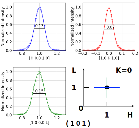
Figure 1: Cuts along H K and L of the elastic (E=0meV) nuclear Bragg peak $(1,0,1)$. Errorbars are contained in the symbol size. Lines are Gaussian fits.

II Magnetic ordering

One can see that the magnetic order develops at quite short range : 5, 9 and 2 unit cells along H, K and L respectively . This is probably due to impuritites in the 1D magnetic structure.

To characterize the magnetic order, similar cuts along H, K and L directions were extracted around the $(1/2,1/2,1/2)$ magnetic Bragg reflection, see Fig 2. As one can see, the magnetic order develops at shorter range than the atomic structure with magnetic correlation lengths of 5, 9 and 2 unit cells along H, K and L respectively. This is probably due to impuritites in the 1D magnetic structure.

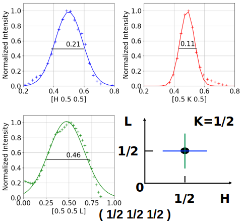
Figure 2: Cuts along H K and L of the elastic (E=0meV) magnetic Bragg peak $(1/2,1/2,1/2)$. Errorbars are contained in the symbol size. Lines are Gaussian fits.

In order to check the sample quality, we fitted the intensity of the $(1/2,1/2,1/2)$ for the three temperatures available, namely 20 K, 100 K and 250 K. Indeed, the Neel temperature is in direct relationship with the sample quality. As can bee seen in Fig. 3, from 20K, to 100 K, the intensity is nearly constant, and is strongly reduced at 250 K, suggesting a T_N close to 200 K as reported in other batches using the very same synthesis conditions (see Fig. 4 in supplementary information of ref. Zheng et al. (2022)). At 250 K, the peak width is sligthly larger with a reduced but non negligable intensity, suggesting a fluctuating magnetic order, compatible with a Neel temperature around 200 K.

As can bee seen in Fig. 3, from 20K, to 100 K, the intensity is nearly constant, and is strongly reduced AT 200 K, suggesting a TN close to 200 K as reported in other batches using the very same synthesis conditions (see FIG 4 in supplementary information of ref. [1]).

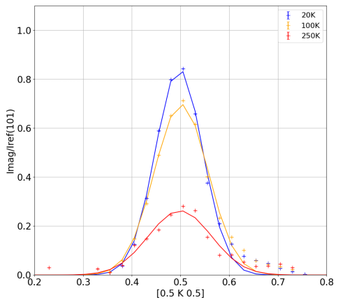
Figure 3: Cuts along K of the elastic (E=0meV) magnetic Bragg peak $(1/2,1/2,1/2)$ for different temperature T=20, 100 and 250 K. Errorbars are contained in the symbol size. Lines are Gaussian fits.

III Anisotropy gap determination

To evidence the anisotropy gap, we removed the elastic contribution to the energy cut at $(1/2,1/2,1/2)$ position from the raw data. The raw data together with the fit is presented in Fig. 4. The background function used in the fit is a combination of a lorentzian fit for the elastic intensity, as well as a background noise with a flat gaussian. The background-substracted intensity is presented in the main manuscript to be compared with simulations.

Figure 4: Intensity at q=$(1/2,1/2,1/2)$ as function of energy (points) with the fitted background (line).

IV Spin wave dispersion along H and L

We extracted the dispersion along H and L around the $(1/2,1/2,1/2)$ magnetic Bragg peak for $E_{i}$=125meV. Using the integration parameters $\Delta K$=0.5 for both maps, and $\Delta H$=0.5 and $\Delta L$=10, the results are presented in Fig. 5. As we can see, no dispersion is visible for both directions, as expected from the short range correlations extracted from the elastic peak along a and c axis of 5 and 2 unit cells respectively.

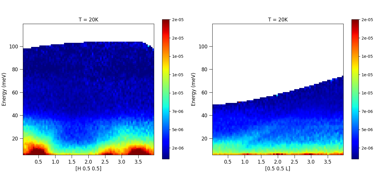
Figure 5: Color map along $(H,1/2,1/2)$ (left) and $(1/2,1/2,L)$ (right) of the dispersion at 20 K ($E_{i}$ = 125  meV), with integration range of $\Delta K$=0.5 $\Delta H$=0.5 and $\Delta L$=10

V Monte-Carlo simulations

Classical Monte-Carlo, with both Metropolis-Hasting algorithm and adaptive method described in Alzate-Cardona et al. (2019), was used to determine the phase diagram of a single ladder. In the calculations, a ladder consisting of 2 legs of 100 spins coupled together was considered, and the simulations were performed with 10 000 Monte Carlo Steps (MCS) to ensure convergence. In these simulations, no simulated annealing was performed and the temperature was set to 0.01 K. The magnetic structure factor $S(Q)$ was then computed, averaging over the ground state configurations sampled by the Metropolis-Hasting algorithm. The propagation vector of the structure was determined based upon the $Q$-value which maximizes $S(Q)$. The Fig.6 shows the calculations of S(Q) for the exchanges couplings of our model: we observe 2 distincts peaks, which are actually the same, because of the periodicity and symmetry of the Brillouin zone. The first peak is centered around k = 0.25, well defined in the main article as the propagation vector of the expected structure.

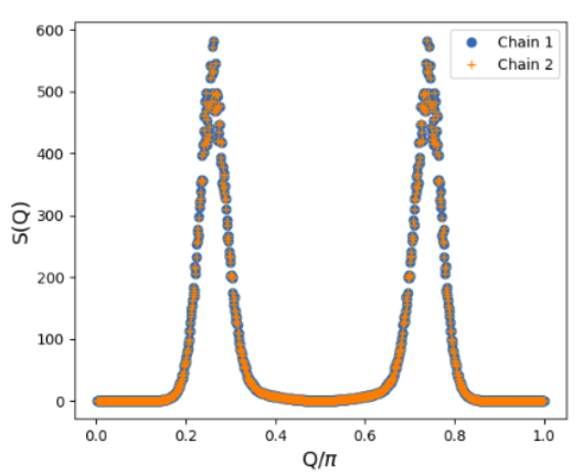
Figure 6: Magnetic structure factor S(Q) for both legs of a ladder with the couplings taken in the main article (see Tab. II).

References

- Zheng et al. (2020) W. Zheng, V. Balédent, M. Lepetit, P. Retailleau, E. Elslande, C. Pasquier, P. Auban-Senzier, A. Forget, D. Colson, and P. Foury-Leylekian, Phys. Rev. B 101, 020101 (2020).
- Zheng et al. (2022) W. G. Zheng, V. Balédent, E. Ressouche, V. Petricek, D. Bounoua, P. Bourges, Y. Sidis, A. Forget, D. Colson, and P. Foury-Leylekian, Phys. Rev. B 106, 134429 (2022).
- Alzate-Cardona et al. (2019) J. Alzate-Cardona, D. Sabogal-Suárez, R. Evans, and E. Restrepo-Parra, Journal of Physics: Condensed Matter 31, 095802 (2019).