Stationarity with Occasionally Binding Constraints

Abstract

This paper studies a class of multivariate threshold autoregressive models, known as censored and kinked structural vector autoregressions (CKSVAR), which are notably able to accommodate series that are subject to occasionally binding constraints. We develop a set of sufficient conditions for the processes generated by a CKSVAR to be stationary, ergodic, and weakly dependent. Our conditions relate directly to the stability of the deterministic part of the model, and are therefore less conservative than those typically available for general vector threshold autoregressive (VTAR) models. Though our criteria refer to quantities, such as refinements of the joint spectral radius, that cannot feasibly be computed exactly, they can be approximated numerically to a high degree of precision. Our results also permit us to provide a treatment of unit roots and cointegration in the CKSVAR, for the case where the model is configured so as to generate linear cointegration.

The results of this paper were first presented in Sections 2, 3 and 4.4.3 of arXiv:2211.09604v1. We thank participants at seminars at Cambridge, Cyprus, Stanford and Oxford, for comments on earlier drafts of this work.

1 Introduction

This paper studies a class of multivariate threshold autoregressive models known as censored and kinked structural vector autoregressions (CKSVAR; SM21). These models feature endogenous regime switching induced by threshold-type nonlinearities, i.e. changes in coefficients and variances when one of the variables crosses a threshold, but differ importantly from a previous generation of vector threshold autoregressive models (VTAR; see e.g. TTG10) insofar as the autoregressive ‘regime’ is determined endogenously, rather than being pre-determined. This notably allows the CKSVAR model to accommodate series that are subject to occasionally binding constraints, a leading example of which is provided by the zero lower bound (ZLB) on short-term nominal interest rates (SM21; AMSV21; ILMZ20).

In this paper, we develop a set of sufficient conditions for the processes generated by the CKSVAR to be stationary, ergodic, and weakly dependent. These conditions are of interest, firstly, because the credibility of a structural model relies on its being able to generate plausible counterfactual trajectories and associated impulse responses, i.e. on its being adequate to replicate the most elementary time series properties of the data. If that data is apparently stationary, model configurations that instead give rise to explosive trajectories and responses should naturally be excluded from the parameter space (in a Bayesian setting, by assigning zero prior mass to these regions; cf. AMSV21, Sec. 3.3). Secondly, frequentist inference on the parameters of these models relies on the series generated by the model, under the null hypothesis of interest, satisfying the requirements of laws of large numbers and central limit theorems for dependent data (Wool94Hdbk; PP97).

Because of the nonlinearity of the CKSVAR, the stationarity of the model defies the simple analytical characterisation that is available in a linear VAR. (In particular, it is insufficient to simply check the magnitudes of the autoregressive roots associated with some or all of the autoregressive ‘regimes’ implied by the model: see 3.1 below.) This is a problem routinely encountered in the literature on nonlinear time series models, and some of the approaches taken in that literature may be fruitfully applied here. Specifically, we rely on existing results from the theory of ergodic Markov processes (Tjo90AAP; MT09), casting the CKSVAR as an instance of the ‘regime switching’ or VTAR models considered in that literature (see e.g. Tong90; Chan09; TTG10; HT13), in order to establish conditions sufficient for the series generated by a CKSVAR to be stationary, ergodic, and $\beta$-mixing (absolutely regular). Because the CKSVAR is continuous at the threshold (kink) and approximately homogeneous (of degree one), this can be characterised directly in terms of the stability of the deterministic part of the model, as per CT85AAP, yielding conditions for stationarity that are less conservative than those available for general VTAR models.

We develop a hierarchy of sufficient conditions for stability, only the most elementary of which, the joint spectral radius (JSR), has previously been applied to nonlinear time series models (e.g. Lieb2005; MS08JTSA; Saik08ET; KS2020ER). Though our criteria refer to quantities that cannot feasibly be computed exactly, they can be approximated numerically to a high degree of precision (arbitrarily well, given sufficient computation time, in some cases); we have developed the R package thresholdr to provide users of these models with a straightforward way of verifying these criteria.

Our results also permit us to provide a limited treatment of unit roots and cointegration in the CKSVAR, for the case where the model is configured so as to generate linear cointegration, and the variable subject to the threshold-type nonlinearity (or occasionally binding constraint) is stationary. While this configuration falls within the domain of the existing literature on nonlinear vector error correction models (see e.g. BF97IER; HS02JoE; Saik05JoE; Saik08ET; KR10JoE; KR13ET), we are able to improve on that literature by exploiting the special structure of the CKSVAR model. For a fuller, complementary development of unit roots and cointegration within this model, which emphasises the possibilities for nonlinear cointegration, the reader is referred to DMW22.

The remainder of the paper is organised as follows. 2 introduces the CKSVAR model and develops a canonical representation of that model, which is particularly amenable to our analysis. In 3, we provide sufficient conditions for the CKSVAR to generate stationary, ergodic and weakly dependent time series. Those depend, in turn, on the stability of the deterministic part of the model, criteria for which are elaborated in 4. With the aid of our results, 5 develops general conditions under which the model accommodates linear cointegration. All proofs appear in the appendices.

Notation.

$e_{m,i}$ denotes the $i$th column of an $m\times m$ identity matrix; when $m$ is clear from the context, we write this simply as $e_{i}$. In a statement such as $f(a^{\pm},b^{\pm})=0$, the notation ‘$\pm$’ signifies that both $f(a^{+},b^{+})=0$ and $f(a^{-},b^{-})=0$ hold; similarly, ‘$a^{\pm}\in A$’ denotes that both $a^{+}$ and $a^{-}$ are elements of $A$. All limits are taken as $n\rightarrow\infty$ unless otherwise stated. $\overset{p}{\rightarrow}$ and $\rightsquigarrow$ respectively denote convergence in probability and in distribution (weak convergence). $\lVert\cdot\rVert$ denotes the Euclidean norm on $\mathbb{R}^{m}$; all matrix norms are induced by the corresponding vector norms. For $X$ a random variable and $p\geq 1$, $\lVert X\rVert_{p}\coloneqq(\mathbb{E}\lvert X\rvert^{p})^{1/p}$.

2 Model

2.1 The censored and kinked SVAR

We study a VAR model which allows one variable, $y_{t}$, to enter differently according to whether it is above or below a time-invariant threshold $b$. Define

$$y_{t}^{+} \coloneqq\max\{y_{t},b\} y_{t}^{-} \coloneqq\min\{y_{t},b\}$$ (2.1)

and consider the model

$$\phi_{0}^{+}y_{t}^{+}+\phi_{0}^{-}y_{t}^{-}+\Phi_{0}^{x}x_{t}=c+\sum_{i=1}^{k}[\phi_{i}^{+}y_{t-i}^{+}+\phi_{i}^{-}y_{t-i}^{-}+\Phi_{i}^{x}x_{t-i}]+u_{t}$$ (2.2)

which we may write more compactly as

$$\phi^{+}(L)y_{t}^{+}+\phi^{-}(L)y_{t}^{-}+\Phi^{x}(L)x_{t}=c+u_{t},$$ (2.3)

where $\phi^{\pm}(\lambda)\coloneqq\phi_{0}^{\pm}-\sum_{i=1}^{k}\phi_{i}^{\pm}\lambda^{i}$ and $\Phi^{x}(\lambda)\coloneqq\Phi_{0}^{x}-\sum_{i=1}^{k}\Phi_{i}^{x}\lambda^{i}$, for $\phi_{i}^{\pm}\in\mathbb{R}^{p\times 1}$ and $\Phi_{i}^{x}\in\mathbb{R}^{p\times(p-1)}$, and $L$ denotes the lag operator. If $b\neq 0$, then by defining $y_{b,t}\coloneqq y_{t}-b$, $y_{b,t}^{+}\coloneqq\max\{y_{b,t},0\}$, $y_{b,t}^{-}\coloneqq\min\{y_{b,t},0\}$ and $c_{b}\coloneqq c-[\phi^{+}(1)+\phi^{-}(1)]b$, we may rewrite (LABEL:var-pm) as

$$\phi^{+}(L)y_{b,t}^{+}+\phi^{-}(L)y_{b,t}^{-}+\Phi^{x}(L)x_{t}=c_{b}+u_{t}.$$ (2.4)

For the purposes of this paper, we may thus take $b=0$ without loss of generality. In this case, $y_{t}^{+}$ and $y_{t}^{-}$ respectively equal the positive and negative parts of $y_{t}$, and $y_{t}=y_{t}^{+}+y_{t}^{-}$. (Throughout the following, the notation ‘$a^{\pm}$’ connotes $a^{+}$ and $a^{-}$ as objects associated respectively with $y_{t}^{+}$ and $y_{t}^{-}$, or their lags. If we want to instead denote the positive and negative parts of some $a\in\mathbb{R}$, we shall do so by writing $[a]_{+}\coloneqq\max\{a,0\}$ and $[a]_{-}\coloneqq\min\{a,0\}$.)

Models of the form of (LABEL:var-pm) have previously been employed in the literature to account for the dynamic effects of censoring, occasionally binding constraints, and endogenous regime switching: see SM21, AMSV21 and ILMZ20. We shall follow SM21 in referring to (LABEL:var-pm) as a censored and kinked structural VAR (CKSVAR) model. The following running example will be used to illustrate the concepts developed in this paper.

Example 2.1 (monetary policy).

Consider the following stylised structural model of monetary policy in the presence of a zero lower bound (ZLB) constraint on interest rates consisting of a composite IS and Phillips curve (PC) equation

$$\pi_{t}-\overline{\pi} =\chi(\pi_{t-1}-\overline{\pi})+\theta[i_{t}^{+}+\mu i_{t}^{-}-(r_{t}^{\ast}+\overline{\pi})]+\varepsilon_{t}$$ (2.5)

and a policy reaction function (Taylor rule)

$$i_{t}=(r_{t}^{\ast}+\overline{\pi})+\gamma(\pi_{t}-\overline{\pi})$$ (2.6)

where $r_{t}^{\ast}$ denotes the (real) natural rate of interest, $\pi_{t}$ inflation, and $\varepsilon_{t}$ a mean zero, i.i.d. innovation. The stance of monetary policy is measured by $i_{t}$: with $i_{t}^{+}=[i_{t}]_{+}$ giving the actual policy rate (constrained to be non-negative), and $i_{t}^{-}$ the desired stance of policy when the policy rate is constrained by the ZLB, to be effected via some form of ‘unconventional’ monetary policy, such as long-term asset purchases. $\overline{\pi}$ denotes the central bank’s inflation target. We maintain that $\gamma>0$, $\theta<0$, $\chi\in[0,1)$, and $\mu\in[0,1]$, where this last parameter captures the relative efficacy of unconventional policy. When $\chi=0$, the preceding corresponds to a simplified version of the model of ILMZ20.

To ‘close’ the model, we specify that the (unobserved) natural real rate of interest follows a stationary AR(1) process,

$$r_{t}^{\ast}=\overline{r}+\psi r_{t-1}^{\ast}+\eta_{t}$$ (2.7)

where $\psi\in(-1,1)$, and $\eta_{t}$ is an i.i.d. mean zero innovation, possibly correlated with $\varepsilon_{t}$ (cf. LW03REStat, for a model in which $\psi=1$). By substituting (LABEL:taylor) into (LABEL:is-pc) and (LABEL:natural-rate), and letting $\overline{\imath}\coloneqq\overline{r}+\overline{\pi}$, we obtain

$$\begin{bmatrix}1&1&-\gamma\\ 0&\theta(1-\mu)&1-\theta\gamma\end{bmatrix}\begin{bmatrix}i_{t}^{+}\\ i_{t}^{-}\\ \pi_{t}\end{bmatrix}=\begin{bmatrix}(1-\psi)(\overline{\imath}-\gamma\overline{\pi})\\ (1-\theta\gamma-\chi)\overline{\pi}\end{bmatrix}+\begin{bmatrix}\psi&\psi&-\psi\gamma\\ 0&0&\chi\end{bmatrix}\begin{bmatrix}i_{t-1}^{+}\\ i_{t-1}^{-}\\ \pi_{t-1}\end{bmatrix}+\begin{bmatrix}\eta_{t}\\ \varepsilon_{t}\end{bmatrix},$$ (2.8)

rendering the system as a CKSVAR for $(i_{t},\pi_{t})$.

The CKSVAR also incorporates both kinds of dynamic Tobit model as special cases (for applications of which, in both time series and panel settings, see e.g. DJ02FRB; DJH11; DSK12AE; LMS19; BMMV21JBF; and Byk21JBES).

Example 2.2 (dynamic Tobit).

Consider (LABEL:var-pm) with $p=1$ and $\phi_{0}^{+}=\phi_{0}^{-}=1$, so that

$$y_{t}=c+\sum_{i=1}^{k}(\phi_{i}^{+}y_{t-i}^{+}+\phi_{i}^{-}y_{t-i}^{-})+u_{t},$$ (2.9)

and suppose only $y_{t}^{+}$ is observed. In the nomenclature of BD22, if $\phi_{i}^{-}=0$ for all $i\in\{1,\ldots,k\}$, so that only the positive part of $y_{t-i}$ enters the r.h.s., then

$$y_{t}^{+}=\left[c+\sum_{i=1}^{k}\phi_{i}^{+}y_{t-i}^{+}+u_{t}\right]_{+}$$ (2.10)

follows a censored dynamic Tobit; whereas if $\phi_{i}^{+}=\phi_{i}^{-}=\phi_{i}$ for all $i\in\{1,\ldots,k\}$, then $y_{t}^{+}$ follows a latent dynamic Tobit, being simply the positive part of the linear autoregression,

$$y_{t}=c+\sum_{i=1}^{k}\phi_{i}y_{t-i}+u_{t}$$ (2.11)

(cf. Maddala83; wei1999).

As discussed by SM21 and AMSV21, the CKSVAR (LABEL:var-pm) is not guaranteed to have a unique solution for $(y_{t},x_{t})$, at least not for all possible values of $u_{t}$, unless certain conditions are placed on entries of the matrix

$$\Phi_{0}\coloneqq\begin{bmatrix}\phi_{0}^{+}&\phi_{0}^{-}&\Phi_{0}^{x}\end{bmatrix}=\begin{bmatrix}\phi_{0,yy}^{+}&\phi_{0,yy}^{-}&\phi_{0,yx}^{\mathsf{T}}\\ \phi_{0,xy}^{+}&\phi_{0,xy}^{-}&\Phi_{0,xx}\end{bmatrix}$$

of contemporaneous coefficients; or equivalently on the matrices

$$\Phi_{0}^{+} \coloneqq\begin{bmatrix}\phi_{0}^{+}&\Phi_{0}^{x}\end{bmatrix} \Phi_{0}^{-} \coloneqq\begin{bmatrix}\phi_{0}^{-}&\Phi_{0}^{x}\end{bmatrix}$$

that respectively apply when $y_{t}$ is positive or negative. By SM21, (LABEL:var-pm) has a unique solution – the model is ‘coherent and complete’ (see also GLM80Ecta) – if the second condition of the following holds.

Assumption DGP.

1. $\{(y_{t},x_{t})\}$ are generated according to (LABEL:y-threshold)–(LABEL:var-pm) with $b=0$, with possibly random initial values $(y_{i},x_{i})$, for $i\in\{-k+1,\ldots,0\}$;

2. $\operatorname{sgn}(\det\Phi_{0}^{+})=\operatorname{sgn}(\det\Phi_{0}^{-})\neq 0$.

3. $\Phi_{0,xx}$ is invertible, and

   $$\operatorname{sgn}\{\phi_{0,yy}^{+}-\phi_{0,yx}^{\mathsf{T}}\Phi_{0,xx}^{-1}\phi_{0,xy}^{+}\}=\operatorname{sgn}\{\phi_{0,yy}^{-}-\phi_{0,yx}^{\mathsf{T}}\Phi_{0,xx}^{-1}\phi_{0,xy}^{-}\}>0.$$ (2.12)

Remark 2.1.

(i). Under DGP.2, a reordering of the equations in (LABEL:var-pm), and thus of the rows of $\Phi_{0}$, ensures $\Phi_{0,xx}$ is invertible. Since $\det(\phi_{0,yy}^{\pm}-\phi_{0,yx}^{\mathsf{T}}\Phi_{0,xx}^{-1}\phi_{0,xy}^{\pm})=\det(\Phi_{0}^{\pm})/\det(\Phi_{0,xx})$, the equality in (LABEL:coherence) holds; the inequality can thus be satisfied by multiplying (LABEL:var-pm) through by $\pm 1$ as appropriate. Thus DGP.3 is without loss of generality, and we have stated it here only to clarify that we shall treat these normalisations as holding, purely for the sake of convenience, throughout the sequel.

(ii). An important special case of the CKSVAR arises when $y_{t}^{-}$ is not observed – or when it is only observed up to scale – in which case there is a continuum of observationally equivalent parametrisations of (LABEL:var-pm), each of which generate identical time series for the observables $(y_{t}^{+},x_{t})$, but in which the trajectories for $y_{t}^{-}$ are scaled by some constant. (In e.g. SM21, this arises because the ‘shadow rate’ is unobservable below zero.) In this case, the scale of the coefficients $\{\phi_{i}^{-}\}_{i=0}^{p}$ on $y_{t}^{-}$ in (LABEL:var-pm) can be normalised in a convenient way that permits certain simplifications to be made; we shall refer to this as the case of a partially observed CKSVAR.

2.2 The canonical CKSVAR

We say that a CKSVAR is canonical if

$$\Phi_{0}=\begin{bmatrix}1&1&0\\ 0&0&I_{p-1}\end{bmatrix}\eqqcolon I_{p}^{\ast},$$ (2.13)

While it is not always the case that the reduced form of (LABEL:var-pm) corresponds directly to a canonical CKSVAR, by defining the canonical variables

$$\begin{bmatrix}\tilde{y}_{t}^{+}\\ \tilde{y}_{t}^{-}\\ \tilde{x}_{t}\end{bmatrix}\coloneqq\begin{bmatrix}\tilde{\phi}_{0,yy}^{+}&0&0\\ 0&\tilde{\phi}_{0,yy}^{-}&0\\ \phi_{0,xy}^{+}&\phi_{0,xy}^{-}&\Phi_{0,xx}\end{bmatrix}\begin{bmatrix}y_{t}^{+}\\ y_{t}^{-}\\ x_{t}\end{bmatrix}\eqqcolon P^{-1}\begin{bmatrix}y_{t}^{+}\\ y_{t}^{-}\\ x_{t}\end{bmatrix},$$ (2.14)

where $\tilde{\phi}_{0,yy}^{\pm}\coloneqq\phi_{0,yy}^{\pm}-\phi_{0,yx}^{\mathsf{T}}\Phi_{0,xx}^{-1}\phi_{0,xy}^{\pm}>0$ and $P^{-1}$ is invertible under DGP; and setting

$$\begin{bmatrix}\tilde{\phi}^{+}(\lambda)&\tilde{\phi}^{-}(\lambda)&\tilde{\Phi}^{x}(\lambda)\end{bmatrix}\coloneqq Q\begin{bmatrix}\phi^{+}(\lambda)&\phi^{-}(\lambda)&\Phi^{x}(\lambda)\end{bmatrix}P,$$ (2.15)

where

$$Q\coloneqq\begin{bmatrix}1&-\phi_{0,yx}^{\mathsf{T}}\Phi_{0,xx}^{-1}\\ 0&I_{p-1}\end{bmatrix},$$ (2.16)

we obtain the following, whose proof appears in A.

Proposition 2.1.

Suppose DGP holds. Then:

1. there exist $(\tilde{y}_{t},\tilde{x}_{t})$ such that (LABEL:canon-vars)–(LABEL:canon-polys) hold, $\tilde{y}_{t}^{+}=\max\{\tilde{y}_{t},0\}$, $\tilde{y}_{t}^{-}=\min\{\tilde{y}_{t},0\}$ and

   $$\tilde{\phi}^{+}(L)\tilde{y}_{t}^{+}+\tilde{\phi}^{-}(L)\tilde{y}_{t}^{-}+\tilde{\Phi}^{x}(L)\tilde{x}_{t}=\tilde{c}+\tilde{u}_{t},$$ (2.17)

   is a canonical CKSVAR, where $\tilde{c}=Qc$ and $\tilde{u}_{t}=Qu_{t}$; and

2. if the CKSVAR for $(y_{t},x_{t})$ is partially observed, $y_{t}^{-}$ may be rescaled such that we may take $\tilde{y}_{t}=y_{t}$.

The utility of the canonical representation lies in its rendering all the nonlinearity in the model as a more tractable function of the lags of $\tilde{y}_{t}$ alone. Because the time-series properties of a general CKSVAR are inherited from its canonical form, we may restrict attention to canonical CKSVAR models essentially without loss of generality. More precisely, for convenience we shall state our results below for canonical CKSVAR models, and then invert the mapping (LABEL:canon-vars)–(LABEL:canon-polys) to determine their implications for general CKSVAR models. That is, we shall initially maintain the following.

Assumption DGP^∗.

$\{(y_{t},x_{t})\}$ are generated by a canonical CKSVAR, i.e. as

$$\phi^{+}(L)y_{t}^{+}+\phi^{-}(L)y_{t}^{-}+\Phi^{x}(L)x_{t}=c+u_{t},$$ (2.18)

with $\Phi_{0}=[\phi_{0}^{+},\phi_{0}^{-},\Phi^{x}]=I_{p}^{\ast}$ (and $b=0$); or equivalently, as

$$\begin{bmatrix}y_{t}\\ x_{t}\end{bmatrix}=c+\sum_{i=1}^{k}\begin{bmatrix}\phi_{i}^{+}&\phi_{i}^{-}&\Phi_{i}^{x}\end{bmatrix}\begin{bmatrix}y_{t-i}^{+}\\ y_{t-i}^{-}\\ x_{t-i}\end{bmatrix}+u_{t},$$ (2.19)

with (possibly random) initial values $(y_{i},x_{i})$, for $i\in\{-k+1,\ldots,0\}$.

Example 2.3 (monetary policy; ctd).

From (LABEL:cksvar-natrate) above we have

$$\Phi_{0}^{+} =\begin{bmatrix}1&-\gamma\\ 0&1-\theta\gamma\end{bmatrix} \Phi_{0}^{-} =\begin{bmatrix}1&-\gamma\\ \theta(1-\mu)&1-\theta\gamma\end{bmatrix},$$

and thus $\det\Phi_{0}^{+}=1-\theta\gamma$ and $\det\Phi_{0}^{-}=1-\mu\theta\gamma$, both of which are positive, so that the coherence condition DGP.2 is satisfied. (The model is already written in a form such that DGP.3 also holds.) The model may be rendered in canonical form by taking

$$\begin{aligned} \begin{bmatrix}\tilde{\imath}_{t}^{+}\\ \tilde{\imath}_{t}^{-}\\ \tilde{\pi}_{t}\end{bmatrix}&\coloneqq\begin{bmatrix}1&0&0\\ 0&1+\tau_{\mu}&0\\ 0&\theta(1-\mu)&1-\theta\gamma\end{bmatrix}\begin{bmatrix}i_{t}^{+}\\ i_{t}^{-}\\ \pi_{t}\end{bmatrix}\qquad&\qquad\begin{bmatrix}\tilde{\eta}_{t}\\ \tilde{\varepsilon}_{t}\end{bmatrix}&\coloneqq\begin{bmatrix}1&\gamma(1-\theta\gamma)^{-1}\\ 0&1\end{bmatrix}\begin{bmatrix}\eta_{t}\\ \varepsilon_{t}\end{bmatrix}\end{aligned}$$ (2.20)

$$\tilde{c}\coloneqq\begin{bmatrix}1&\gamma(1-\theta\gamma)^{-1}\\ 0&1\end{bmatrix}\begin{bmatrix}(1-\psi)(\overline{\imath}-\gamma\overline{\pi})\\ (1-\theta\gamma-\chi)\overline{\pi}\end{bmatrix}$$ (2.21)

where $\tau_{\mu}\coloneqq\gamma\theta(1-\mu)(1-\theta\gamma)^{-1}$, for which it holds that

$$\begin{bmatrix}\tilde{\imath}_{t}\\ \tilde{\pi}_{t}\end{bmatrix}=\tilde{c}+\begin{bmatrix}\psi&\psi-\chi\tau_{\mu}\kappa_{\mu}&\gamma(\chi\kappa_{1}-\psi)\kappa_{1}\\ 0&-\chi\theta(1-\mu)\kappa_{\mu}&\chi\kappa_{1}\end{bmatrix}\begin{bmatrix}\tilde{\imath}_{t-1}^{+}\\ \tilde{\imath}_{t-1}^{-}\\ \tilde{\pi}_{t-1}\end{bmatrix}+\begin{bmatrix}\tilde{\eta}_{t}\\ \tilde{\varepsilon}_{t}\end{bmatrix}$$ (2.22)

where $\kappa_{\mu}\coloneqq(1-\mu\theta\gamma)^{-1}$.

3 Stationarity and ergodicity

3.1 The CKSVAR as a regime-switching model

The nonlinearity of the CKSVAR makes the assessment of its stationarity a rather more complicated affair than it is for a linear (S)VAR. Though it may be natural to think of the model as having two autoregressive ‘regimes’, corresponding respectively to positive and negative values of $\{y_{t}\}$, and associated with the autoregressive polynomials

$$\Phi^{\pm}(\lambda)\coloneqq\begin{bmatrix}\phi^{\pm}(\lambda)&\Phi^{x}(\lambda)\end{bmatrix},$$

the roots of $\Phi^{\pm}(\lambda)$ are not sufficient to characterise the stationarity of the model. What seems an intuitive criterion for stationarity, that all these roots should lie outside the unit circle, turns out to be neither necessary nor sufficient – at best, it is merely necessary for another criterion for stability to be satisfied, as we develop below. Even in very special cases, such as a CKSVAR in which only lags of $y_{t}^{+}$ enter the model (as e.g. in AMSV21), it is possible to construct numerical examples of the following kind.

Example 3.1 (explosive).

Consider a CKSVAR with $p=3$ and $k=1$, where $\Phi_{0}=I_{3}^{\ast}$ and

$$\phi_{1}^{+} =\begin{bmatrix}-1.37\\ 0.79\\ 0.76\end{bmatrix} \phi_{1}^{-} =\begin{bmatrix}0\\ 0\\ 0\end{bmatrix} \Phi_{1}^{x} =\begin{bmatrix}-1.00&0.36\\ 0.39&-1.33\\ 0.71&0.03\end{bmatrix},$$

and $c=0$. The model has only two autoregressive regimes, associated with the autoregressive matrices $\Phi^{+}=[\phi_{1}^{+},\Phi_{1}^{x}]$ and $\Phi^{-}=[\phi_{1}^{-},\Phi_{1}^{x}]$; it may be verified that the eigenvalues of each lie inside the unit circle, with the largest (in modulus) being $0.85$ and $0.98$ respectively. Nonetheless, the simulated trajectories generated by this model are clearly explosive (for plots of $\{y_{t}\}$ when the model is simulated with $\Sigma=I_{3}$, see 3.1). The reason for this is that both $\Phi^{+}$ and $\Phi^{-}$ have a pair of complex eigenvalues, which causes the sign of $y_{t}$ to continually oscillate – with the result that the evolution of $(y_{t},x_{t})$ is governed by $\Phi^{+}\Phi^{-}$, whose largest eigenvalue lies outside the unit circle.

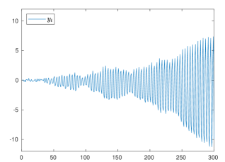
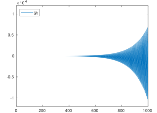
Figure 3.1: Simulated trajectories for the CKSVAR in 3.1

As the above example illustrates, a tractable analytic characterisation of stationarity is unlikely to be available in this setting. To make progress we draw on approaches developed in the literature on nonlinear time series models, specifically those pertaining to ‘regime switching’ or ‘vector threshold autoregressive’ (VTAR) models (see HT13), of which the CKSVAR is an instance. To make this more apparent, let $\mathbf{1}^{+}(y)\coloneqq\mathbf{1}\{y\geq 0\}$ and $\mathbf{1}^{-}(y)\coloneqq\mathbf{1}\{y<0\}$, and define

$$\phi_{i}(y) \coloneqq\phi_{i}^{+}\mathbf{1}^{+}(y)+\phi_{i}^{-}\mathbf{1}^{-}(y) \Phi_{i}(y) \coloneqq\begin{bmatrix}\phi_{i}(y)&\Phi_{i}^{x}\end{bmatrix}$$

for $i\in\{1,\ldots,k\}$. Then for $z_{t}\coloneqq(y_{t},x_{t}^{\mathsf{T}})^{\mathsf{T}}$, the canonical CKSVAR

$$z_{t}=c+\sum_{i=1}^{k}\Phi_{i}(y_{t-i})z_{t-i}+u_{t}$$ (3.1)

may be regarded as an autoregressive model with $2^{k}$ ‘regimes’ corresponding to all the possible sign patterns of $(y_{t-1},\ldots,y_{t-k})$, with switches between those regimes occurring at each of the $k$ ‘thresholds’ defined by $y_{t-i}=0$. While the existing literature provides results on the stationarity of a general class of regime-switching vector autoregressive models (see e.g. Lieb2005; Saik08ET; KS2020ER), because of that very generality we are able to improve on those results by exploiting the special structure of a CKSVAR model.

3.2 Ergodicity via stability of the deterministic subsystem

To state our results, we first recall the following (cf. Lieb2005, p. 671).

Definition 3.1.

Let $\{w_{t}\}_{t\in\mathbb{N}_{0}}$ be a Markov chain taking values in $\mathbb{R}^{d_{w}}$, with $m$-step transition kernel $P^{m}(w,A)\coloneqq\mathbb{P}\{w_{t+m}\in A\mid w_{t}=w\}$, and $\mathcal{Q}:\mathbb{R}^{d_{w}}\rightarrow\mathbb{R}_{+}$. We say that $\{w_{t}\}$ is $\mathcal{Q}$-geometrically ergodic, with stationary distribution $\pi$, if $\int_{\mathbb{R}^{d_{w}}}\mathcal{Q}(w)\pi(\mathrm{d}w)<\infty$, and there exist $a,b>0$ and $\gamma\in(0,1)$ such that

$$\sup_{B\in\mathcal{B}}\lvert P^{m}(w,B)-\pi(B)\rvert\leq(a+b\mathcal{Q}(w))\gamma^{m}$$

for all $w\in\mathbb{R}^{d_{w}}$, where $\mathcal{B}$ denotes the Borel sigma-field on $\mathbb{R}^{d_{w}}$.

If $\{w_{t}\}$ is $\mathcal{Q}$-geometrically ergodic, it will be stationary if given a stationary initialisation, i.e. if $w_{0}$ also has distribution $\pi$; moreover, it will have geometrically decaying $\beta$-mixing coefficients. For these and further properties of such sequences, and a discussion of how this concept relates to other notions of ergodicity used in the literature, see Lieb2005. Since it is the only kind of ergodicity used in this paper, we will use ‘ergodic’ as a shorthand for ‘$\mathcal{Q}$-geometrically ergodic’ in the sequel.

While $\{z_{t}\}$ is not a Markov chain, $\boldsymbol{z}_{t}\coloneqq(z_{t}^{\mathsf{T}},\ldots,z_{t-k+1}^{\mathsf{T}})^{\mathsf{T}}$ trivially is, as can be seen by rendering (LABEL:regimeswitching) in companion form. To establish that $\{\boldsymbol{z}_{t}\}$ is ergodic, we shall make the following assumption on the innovation sequence $\{u_{t}\}$ in (LABEL:var-pm), which allows for a certain form of conditional heteroskedasticity.

Assumption ERR.

$u_{t}=\Sigma(\boldsymbol{z}_{t-1})\varepsilon_{t}$, where

1. $\{\varepsilon_{t}\}$ is i.i.d. and independent of $\boldsymbol{z}_{t-1}$, with a Lebesgue density that is bounded away from zero on compact subsets of $\mathbb{R}^{p}$, and $\mathbb{E}\lVert\varepsilon_{t}\rVert^{m_{0}}<\infty$ for some $m_{0}\geq 1$;

2. for each compact $K\subset\mathbb{R}^{kp}$, there exist $c_{0},c_{1}\in(0,\infty)$ such that the eigenvalues of $\Sigma(\boldsymbol{z})$ lie in $[c_{0},c_{1}]$ for all $\boldsymbol{z}\in K$; and

3. $\Sigma_{ij}(\boldsymbol{z})=o(\lVert\boldsymbol{z}\rVert)$ as $\lVert\boldsymbol{z}\rVert\rightarrow\infty$, for each $i,j\in\{1\ldots,p\}$.

Remark 3.1.

ERR.1 is a standard assumption in this setting, ensuring that the chain is irreducible and that its stationary distribution is continuous (c.f. Lieb2005, p. 675, or Saik08ET, Ass. 1). ERR.2 and ERR.3 are equivalent to (11) and (10) in Lieb2005.

We may now state our main result on the ergodicity of the CKSVAR, which relates the ergodicity of $\{\boldsymbol{z}_{t}\}$ to the stability of deterministic subsystem (or ‘skeleton’ in the terminology of Tong90) of (LABEL:regimeswitching), defined by

$$\hat{z}_{t}=\sum_{i=1}^{k}\Phi_{i}(\hat{y}_{t-i})\hat{z}_{t-i}.$$ (3.2)

We say that such a system is stable if $\hat{z}_{t}\rightarrow 0$ as $t\rightarrow\infty$, for every initialisation $\{\hat{z}_{t}\}_{t=-k+1}^{0}$. Our results for the CKSVAR follow as a corollary to a more general result for continuous and homogeneous (of degree one) autoregressive systems, given as B.2 in B. This in turn extends a fundamental result due to CT85AAP to the present setting, principally by relaxing their conditions on the innovations $\{u_{t}\}$. The proof of the following appears in B.

Theorem 3.1.

Suppose DGP^∗ and ERR hold, and that the deterministic subsystem (LABEL:determ) of the model is stable. Then $\{\boldsymbol{z}_{t}\}_{t\in\mathbb{N}_{0}}$ is $\mathcal{Q}$-geometrically ergodic, for $\mathcal{Q}(\boldsymbol{z})\coloneqq 1+\lVert\boldsymbol{z}\rVert^{m_{0}}$, with a stationary distribution that is absolutely continuous with respect to Lebesgue measure and has finite $m_{0}$th moment.

Remark 3.2.

(i). Suppose that $\{\boldsymbol{z}_{t}\}_{t\in\mathbb{N}_{0}}$ were generated by a structural CKSVAR, i.e. that DGP held in place of DGP^∗. In view of 2.1, $\{\boldsymbol{z}_{t}\}_{t\in\mathbb{N}_{0}}$ is ergodic if and only if the derived canonical process $\{\tilde{\boldsymbol{z}}_{t}\}_{t\in\mathbb{N}_{0}}$ is ergodic. Thus in the general case, the ergodicity of a CKSVAR may be assessed by applying 3.1 to its derived canonical form.

(ii). In view of B.2, the preceding would also hold if the CKSVAR model were generalised by allowing the intercept to vary as $c=c(\boldsymbol{z}_{t-1})$, provided that $c=o(\lVert\boldsymbol{z}\rVert)$ as $\lVert\boldsymbol{z}\rVert\rightarrow\infty$.

(iii). The result holds trivially in a linear VAR, being a special case of the CKSVAR. However, whereas the stability of a linear VAR can be determined from its autoregressive roots, assessing the stability of a CKSVAR requires more elaborate criteria, as developed in the next section.

4 Sufficient conditions for stability

While the preceding reduces the problem to one of verifying the stability of the deterministic subsystem (LABEL:determ), this still presents a formidable challenge. We therefore develop some sufficient conditions for stability – and hence for ergodicity – that can be evaluated numerically. Some of these concepts, particularly the joint spectral radius, have been previously applied to regime-switching and VTAR models, and to this extent there is an overlap between our results and those of Lieb2005 and KS2020ER. However, by exploiting the close connection between the ergodicity of a CKSVAR and the stability of its deterministic subsystem, as per 3.1, we can assess ergodicity using less conservative criteria than are available when working with a broader class of regime-switching autoregressive processes.

4.1 In the abstract

To formulate the criteria in abstract terms, let $\{w_{t}\}_{t\in\mathbb{N}_{0}}$ be a deterministic process, taking values in $\mathbb{R}^{d_{w}}$, that evolves according to a switched linear system: that is, a system in which there is a (possibly uncountable) set ${\cal I}\ni i$ of states, each of which is associated to a distinct autoregressive matrix $A[i]$. If $\{i_{t}\}\subset{\cal I}$ records the state of the system at each $t\in\mathbb{N}_{0}$, then $\{w_{t}\}$ evolves as

$$w_{t}=A[i_{t-1}]w_{t-1}$$ (4.1)

from some given $w_{0}\in\mathbb{R}^{d_{w}}$. Suppose further that the state in period $t$ is entirely determined by the value of $w_{t}$, via the mapping $\sigma:\mathbb{R}^{d_{w}}\rightarrow{\cal I}$. Then $i_{t}=\sigma(w_{t})$, and

$$w_{t}=A[\sigma(w_{t-1})]w_{t-1}\eqqcolon A(w_{t-1})w_{t-1}$$ (4.2)

Let ${\cal A}\coloneqq\{A[i]\}_{i\in{\cal I}}$ denote the set of autoregressive matrices, and $\mathscr{W}_{i}\coloneqq\sigma^{-1}(i)$, so that $\{\mathscr{W}_{i}\}_{i\in{\cal I}}$ partitions $\mathbb{R}^{d_{w}}$.

We say (LABEL:detsystem) is stable if $w_{t}\rightarrow 0$ as $t\rightarrow\infty$, for every $w_{0}\in\mathbb{R}^{d_{w}}$ (what is more precisely termed ‘global asymptotic stability’; e.g. Ela05, pp. 176f.). The usual approach to establishing the stability of such a system is to construct a Lyapunov function. For our purposes, we may take this to be a function $V$ and an associated value $\gamma_{V}\in\mathbb{R}_{+}$ such that

1. $c_{0}\lVert w\rVert\leq V(w)$ for all $w\in\mathbb{R}^{d_{w}}$, for some $c_{0}\in(0,\infty)$; and

2. $V[A(w)w]\leq\gamma_{V}V(w)$ for all $w\in\mathbb{R}^{d_{w}}$.

As is well known, if we can find a $(V,\gamma_{V})$ with $\gamma_{V}<1$, the system is stable (Ela05, Thm. 4.2): and thus the problem of establishing the stability of (LABEL:detsystem) can be reformulated as one of showing that the stability degree $\gamma^{\ast}\coloneqq\inf\{\gamma_{V}\in\mathbb{R}_{+}\mid(V,\gamma_{V})\text{ satisfy (i)--(ii)}\}$ of the system is strictly less than unity. (While stability may be established using a Lyapunov function satisfying weaker conditions than (i)–(ii), for the systems considered here these conditions are not restrictive: see B.1)

While the calculation of $\gamma^{\ast}$ is in general an undecidable problem, various upper bounds for it are known. The most elementary of these is provided by the joint spectral radius (JSR), which for a bounded collection of matrices may be defined as (see e.g. Jungers09, Defn. 1.1)

$$\rho_{{\scriptstyle\mathrm{JSR}}}(\mathcal{A})\coloneqq\limsup_{t\rightarrow\infty}\sup_{B\in\mathcal{A}^{t}}\rho(B)^{1/t}$$

where $\rho(B)$ denotes the spectral radius of $B$, and $\mathcal{A}^{t}\coloneqq\{\prod_{s=1}^{t}M_{s}\mid M_{s}\in\mathcal{A}\}$ is the collection of all possible $t$-fold products of matrices in ${\cal A}$. For each $\epsilon>0$, there exists a norm $\lVert\cdot\rVert_{\ast}$ such that

$$\lVert A[i]w\rVert_{\ast}\leq[\rho_{{\scriptstyle\mathrm{JSR}}}(\mathcal{A})+\epsilon]\lVert w\rVert_{\ast},\ \forall w\in\mathbb{R}^{d_{w}},\ \forall i\in{\cal I},$$ (4.3)

(see e.g. Jungers09, Prop. 1.4) whence $V(w)\coloneqq\lVert w\rVert_{\ast}$ trivially yields a valid Lyapunov function, and so $\gamma^{\ast}\leq\rho_{{\scriptstyle\mathrm{JSR}}}(\mathcal{A})$. Note that $\sup_{i\in{\cal I}}\rho(A[i])$ provides only a lower bound on $\rho_{{\scriptstyle\mathrm{JSR}}}(\mathcal{A})$, so control over the individual spectral radii is necessary, but not sufficient, for control over the JSR of ${\cal A}$.

The conservativeness of the JSR is readily apparent from the fact that it implies the stability of (LABEL:unresdet) irrespective of the sequence $\{i_{t}\}$, so that a system adjudged to be stable by this criterion would remain so even if $\sigma$ were replaced by an arbitrary mapping $\sigma^{\prime}:\mathbb{R}^{d_{w}}\rightarrow{\cal I}$. The JSR can thus be immediately improved upon by taking account of the constraints on the sequence $\{i_{t}\}$ of states permitted by the system. Suppose now that ${\cal I}$ is finite, and let ${\cal J}\subset{\cal I}\times{\cal I}$ denote the set of all pairs $(i,j)$ such that state $i$ may be followed by state $j$, i.e. $(i,j)\in{\cal J}$ if there exists a $w\in\mathscr{W}_{i}$ such that $A[\sigma(w)]w\in\mathscr{W}_{j}$; we say that $\{i_{t}\}$ is admissible by ${\cal J}$ if $(i_{t},i_{t+1})\in{\cal J}$ for all $t$. Then the constrained joint spectral radius (CJSR) may be defined as (cf. Dai12LAA, Defn. 1.2 and Thm. A; PEDJ16Auto, p. 243)

$$\rho_{{\scriptstyle\mathrm{CJSR}}}(A[\cdot];{\cal J})\coloneqq\limsup_{t\rightarrow\infty}\sup_{B\in\mathcal{A}^{t}({\cal J})}\rho(B)^{1/t}$$ (4.4)

where now $\mathcal{A}^{t}({\cal J})\coloneqq\{\prod_{s=1}^{t}A[i_{s}]\mid\{i_{s}\}\text{ is admissible by }\mathcal{J}\}$. By PEDJ16Auto, for each $\epsilon>0$ there exists a family of norms $\{\lVert\cdot\rVert_{i}\}_{i\in\mathcal{I}}$ such that

$$\lVert A[i]w\rVert_{j}\leq[\rho_{{\scriptstyle\mathrm{CJSR}}}(\mathcal{A};{\cal J})+\epsilon]\lVert w\rVert_{i},\ \forall w\in\mathbb{R}^{d_{w}},\ \forall(i,j)\in{\cal J}$$ (4.5)

whence $V(w)\coloneqq\sum_{i\in\mathcal{I}}\lVert w\rVert_{i}\mathbf{1}\{w\in\mathscr{W}_{i}\}$ is a Lyapunov function; it is evident that $\rho_{{\scriptstyle\mathrm{CJSR}}}(A[\cdot];{\cal J})\leq\rho_{{\scriptstyle\mathrm{JSR}}}(\mathcal{A})$, so that the CJSR yields an improved estimate of the stability degree of the system.

The form of the Lyapunov function implicitly provided by the CJSR in turn suggests how this construction may be further improved upon. For $V(w)=\sum_{i\in\mathcal{I}}\lVert w\rVert_{i}\mathbf{1}\{w\in\mathscr{W}_{i}\}$ to be a Lyapunov function, it is sufficient that: (i) such an inequality as (LABEL:cjsr-norms) hold only for $w\in\mathscr{W}_{i}$ such that $A[i]w\in\mathscr{W}_{j}$, rather than for all $w\in\mathbb{R}^{d_{w}}$; and (ii) each $\lVert\cdot\rVert_{i}$ satisfy $\lVert w\rVert_{i}>c_{i}\lVert w\rVert$ on $w\in\mathscr{W}_{i}$, for some $c_{i}>0$, i.e. $\lVert\cdot\rVert_{i}$ need not itself be a norm. Relaxing (LABEL:cjsr-norms) in this manner, and replacing each norm $\lVert\cdot\rVert_{i}$ by some mapping $\mathopen{\hbox{\set@color${\langle}$}\kern-1.94444pt\leavevmode\hbox{\set@color${\langle}$}}\cdot\mathclose{\hbox{\set@color${\rangle}$}\kern-1.94444pt\leavevmode\hbox{\set@color${\rangle}$}}_{i}:\mathbb{R}^{d_{w}}\rightarrow\mathbb{R}$ drawn from a class of functions ${\cal C}$, leads us to define the relaxed joint spectral radius (RJSR) for class ${\cal C}$ as

$$\rho_{{\scriptstyle\mathrm{RJSR}},{\cal C}}(A[\cdot];\mathcal{J},\{\mathscr{W}_{i}\}) \coloneqq\inf\{\gamma\in\mathbb{R}_{+}\mid\exists\{\mathopen{\hbox{\set@color${\langle}$}\kern-1.94444pt\leavevmode\hbox{\set@color${\langle}$}}\cdot\mathclose{\hbox{\set@color${\rangle}$}\kern-1.94444pt\leavevmode\hbox{\set@color${\rangle}$}}_{i},c_{i}\}_{i\in{\cal I}}\ \text{s.t.}\,\mathopen{\hbox{\set@color${\langle}$}\kern-1.94444pt\leavevmode\hbox{\set@color${\langle}$}}\cdot\mathclose{\hbox{\set@color${\rangle}$}\kern-1.94444pt\leavevmode\hbox{\set@color${\rangle}$}}_{i}\in\mathcal{C},\ \forall i\in{\cal I};$$ (4.6)

$$\qquad\qquad c_{i}\lVert w\rVert\leq\mathopen{\hbox{\set@color${\langle}$}\kern-1.94444pt\leavevmode\hbox{\set@color${\langle}$}}w\mathclose{\hbox{\set@color${\rangle}$}\kern-1.94444pt\leavevmode\hbox{\set@color${\rangle}$}}_{i},\ \forall w\in\mathscr{W}_{i},\ \forall i\in{\cal I};\text{ and }$$

$$\qquad\qquad\mathopen{\hbox{\set@color${\langle}$}\kern-1.94444pt\leavevmode\hbox{\set@color${\langle}$}}A[i]w\mathclose{\hbox{\set@color${\rangle}$}\kern-1.94444pt\leavevmode\hbox{\set@color${\rangle}$}}_{j}\leq\gamma\mathopen{\hbox{\set@color${\langle}$}\kern-1.94444pt\leavevmode\hbox{\set@color${\langle}$}}w\mathclose{\hbox{\set@color${\rangle}$}\kern-1.94444pt\leavevmode\hbox{\set@color${\rangle}$}}_{i},\ \forall w\in\mathscr{W}_{i}\text{ s.t. }A[i]w\in\mathscr{W}_{j},\ \forall(i,j)\in{\cal J}\}.$$

Clearly the preceding provides an upper bound for $\gamma^{\ast}$. Whether it provides a lower bound for $\rho_{{\scriptstyle\mathrm{CJSR}}}(A[\cdot];{\cal J})$ depends on the choice of $\mathcal{C}$; this is the case if e.g. $\mathcal{C}$ is taken to be the set of norms on $\mathbb{R}^{d_{w}}$, or some class capable of approximating these norms arbitrarily well (such as homogeneous polynomials).

In practice, the main difficulty with all of these objects is computational, with the exact computation of the (C)JSR known to be an NP–hard problem. Nonetheless, significant progress has been made in calculating approximate upper bounds for both of these quantities, with an (in principle) arbitrarily high degree of accuracy (PJ08LAA; LPJ19ITAC; LPJ20SJCO), using semi-definite (SDP) and sum of squares (SOS) programming. With respect to approximating the RJSR, there is naturally the risk of choosing ${\cal C}$ to be too broad a class of functions that the approximation of $\rho_{{\scriptstyle\mathrm{RJSR}},{\cal C}}$ becomes infeasible. As explained in C, building on the approach of FTCMM02Auto, we therefore take as our starting point the SDP and SOS programs used to approximate the (C)JSR, relaxing the analogues of (LABEL:cjsr-norms) in the direction of (LABEL:RSR), for the case where the $\{\mathscr{W}_{i}\}_{i\in{\cal I}}$ are convex cones (as is appropriate for a CKSVAR). This entails relating ${\cal C}$ to either a certain class of quadratic functions (for the SDP program) or homogeneous polynomials of a given (even) order (for the SOS program), and has the additional benefit that our approximate calculations of $\rho_{{\scriptstyle\mathrm{RJSR}},{\cal C}}$ are guaranteed to provide a lower bound on the estimate of the $\rho_{{\scriptstyle\mathrm{CJSR}}}$ yielded by these programs, and thus a less conservative estimate of $\gamma^{\ast}$ in practice. All of these quantities are calculated by our R package, thresholdr.

4.2 In the CKSVAR

In the present setting, the role of (LABEL:detsystem) is played by (LABEL:determ), the deterministic subsystem of a canonical CKSVAR, rendered here in companion form (and suppressing the ‘hat’ decorations) as

$$\boldsymbol{z}_{t}=\boldsymbol{F}(\boldsymbol{y}_{t-1})\boldsymbol{z}_{t-1}=\boldsymbol{F}[\sigma(\boldsymbol{y}_{t-1})]\boldsymbol{z}_{t-1}=\sum_{i\in{\cal I}}\boldsymbol{F}[i]\mathbf{1}\{\boldsymbol{z}_{t-1}\in\mathscr{Z}_{i}\}\boldsymbol{z}_{t-1},$$ (4.7)

where $\boldsymbol{y}_{t-1}=(y_{t-1},\ldots,y_{t-k})^{\mathsf{T}}$, and

$$\boldsymbol{F}(\boldsymbol{y}_{t-1})\coloneqq\begin{bmatrix}\Phi_{1}(y_{t-1})&\cdots&\Phi_{k-1}(y_{t-k+1})&\Phi_{k}(y_{t-k})\\ I_{p}\\ &\ddots\\ &&I_{p}\end{bmatrix}.$$

Here there are (at most) $\lvert{\cal I}\rvert=2^{k}$ distinct states. If we associate with each $i\in{\cal I}$ a distinct $s(i)\in\{-1,+1\}^{k}$, we can take

$$\mathscr{Z}_{i}\coloneqq\{\boldsymbol{y}_{t-1}\in\mathbb{R}^{k}\mid\mathbf{1}^{+}(y_{t-j})=s_{j}(i),\ \forall j\in\{1,\ldots,k\}\}\times\mathbb{R}^{p-1},$$

$\sigma(\boldsymbol{z}_{t-1})=i$ if $\boldsymbol{z}_{t-1}\in\mathscr{Z}_{i}$, and $\boldsymbol{F}[i]$ to be the autoregressive matrix that applies in this case.

Letting ${\cal F}\coloneqq\{\boldsymbol{F}[i]\}_{i\in{\cal I}}$, the JSR of ${\cal F}$ provides a first estimate of stability degree $\gamma^{\ast}$ of the system. However, since the sign pattern of the first $k-1$ elements of $\boldsymbol{y}_{t-1}$ must propagate forwards to $\boldsymbol{y}_{t}$, any given state $i\in{\cal I}$ can only be succeeded by two other states (which differ only according to the sign of $y_{t}$). Thus we can generally obtain a tighter estimate via the CJSR, which reduces the set of possible transitions from the $\lvert{\cal I}\rvert^{2}=2^{2k}$ implicitly permitted by the calculation of the JSR, to $2\lvert{\cal I}\rvert=2^{k+1}$. An even lower estimate of $\gamma^{\ast}$ – which may prove decisive for establishing the stability of (LABEL:detCKSVAR) – can be obtained via the RJSR, at the cost of greater computation time. 3.1 thus has a noteworthy advantage over approaches that utilise bounds on the (C)JSR to directly establish the ergodicity of the corresponding stochastic system, because the evolution of the deterministic system may be much more tightly constrained, particularly when the innovations $\{u_{t}\}$ have full support, as assumed in ERR.

For especially tractable instances of the CKSVAR, additional sufficient conditions for the stability of (LABEL:detCKSVAR) may also be available. For example, a result of DJH11 implies that for the censored dynamic Tobit ((LABEL:censored-Tobit) above), a sufficient condition for stability is that the ‘censored’ autoregressive polynomial $1-\sum_{i=1}^{k}[\phi_{i}^{+}]_{+}\lambda^{i}$ should have all its roots outside the unit circle. (Interestingly, as their result indicates, control over the the roots of the various autoregressive regimes is not even necessary to ensure the stability of a CKSVAR.)

Example 4.1 (monetary policy; ctd).

From the canonical representation (LABEL:example-canon) of the model, we have

$$\tilde{\Phi}_{1}^{+} =\begin{bmatrix}\psi&\gamma(\chi\kappa_{1}-\psi)\kappa_{1}\\ 0&\chi\kappa_{1}\end{bmatrix} \tilde{\Phi}_{1}^{-} =\begin{bmatrix}\psi-\chi\tau_{\mu}\kappa_{\mu}&\gamma(\chi\kappa_{1}-\psi)\kappa_{1}\\ -\chi\theta(1-\mu)\kappa_{\mu}&\chi\kappa_{1}\end{bmatrix},$$

the stability of which cannot be assessed simply by a consideration of the eigenvalues of these matrices; this must instead be done numerically via the criteria developed above. An exception arises in the special case where $\chi=0$, in which case the canonical form of the model is in fact linear: so these matrices coincide, and have eigenvalues of $0$ and $\psi$. In that case, $(\tilde{\imath}_{t},\tilde{\pi}_{t})$, and therefore $(i_{t},\pi_{t})$, is ergodic if $\lvert\psi\rvert<1$.

5 Linear cointegration in the CKSVAR

The preceding approach may also be adapted to analyse the CKSVAR with unit roots. To that end, define the autoregressive polynomials

$$\Phi^{\pm}(\lambda)\coloneqq\begin{bmatrix}\phi^{\pm}(\lambda)&\Phi^{x}(\lambda)\end{bmatrix},$$

and let $\Gamma_{i}^{\pm}\coloneqq-\sum_{j=i+1}^{k}\Phi_{j}^{\pm}\eqqcolon[\gamma_{i}^{\pm},\Gamma^{x}]$ for $i\in\{1,\ldots,k-1\}$, so that $\Gamma^{\pm}(\lambda)\coloneqq\Phi_{0}^{\pm}-\sum_{i=1}^{k-1}\Gamma_{i}^{\pm}\lambda^{i}$ is such that

$$\Phi^{\pm}(\lambda)=\Phi^{\pm}(1)\lambda+\Gamma^{\pm}(\lambda)(1-\lambda)$$

(cf. Lut07, pp. 248f.). Set $\pi^{\pm}\coloneqq-\phi^{\pm}(1)$ and $\Pi^{x}\coloneqq-\Phi^{x}(1)$. Then we can write the CKSVAR in the form of a vector error correction model (VECM) as

$$\Phi_{0}\begin{bmatrix}\Delta y_{t}^{+}\\ \Delta y_{t}^{-}\\ \Delta x_{t}\end{bmatrix}=c+\begin{bmatrix}\pi^{+}&\pi^{-}&\Pi^{x}\end{bmatrix}\begin{bmatrix}y_{t-1}^{+}\\ y_{t-1}^{-}\\ x_{t-1}\end{bmatrix}+\sum_{i=1}^{k-1}\begin{bmatrix}\gamma_{i}^{+}&\gamma_{i}^{-}&\Gamma_{i}^{x}\end{bmatrix}\begin{bmatrix}\Delta y_{t-i}^{+}\\ \Delta y_{t-i}^{-}\\ \Delta x_{t-i}\end{bmatrix}+u_{t},$$ (5.1)

where $\Delta\coloneqq 1-L$ denotes the difference operator, and for clarity we note that e.g. $\Delta y_{t}^{+}=y_{t}^{+}-y_{t-1}^{+}$ (rather than this being the positive part of $\Delta y_{t}$). Let $\Pi^{\pm}=[\pi^{\pm},\Pi^{x}]$.

5.1 In the canonical form

Because of its greater tractability, we initially consider a CKSVAR in canonical form, so that $\Phi_{0}=I_{p}^{\ast}$ and the l.h.s. of (LABEL:vecm) reduces to $[\begin{smallmatrix}\Delta y_{t}\\ \Delta x_{t}\end{smallmatrix}]$. In this setting, analogously to a linear cointegrated VAR with $I(1)$ variables, some of whose linear combinations are $I(0)$ (see Joh95, Ch. 4), we maintain the following.

Assumption CVAR.

1. $\det\Phi^{\pm}(\lambda)$ has $q^{\pm}$ roots at unity, and all others outside the unit circle;

2. $\operatorname{rk}\Pi^{\pm}=r^{\pm}=p-q^{\pm}$; and

3. $c\in\operatorname{sp}\Pi^{+}\cap\operatorname{sp}\Pi^{-}$.

Within the framework of CVAR, DMW22 develop an exhaustive typology of the forms of cointegration accommodated by the CKSVAR, showing in particular that when some of the common trends in the system load onto $y_{t}$, the model generates varieties of nonlinear cointegration that have not previously appeared in the literature. The analysis of those cases requires new technical results, and so falls outside the scope of this paper. Here we instead consider the case where the model generates purely linear cointegration, in the presence of nonlinear short-run dynamics. This arises when there are $q^{+}=q^{-}=q$ common trends that load entirely onto $x_{t}$, among whose elements there are $r=p-q$ cointegrating relations (what DMW22, term case (iii) cointegration). In terms of the VECM (LABEL:vecm), this corresponds to the matrices $\Pi^{\pm}=[\pi^{\pm},\Pi^{x}]$ having a common rank $r^{+}=r^{-}=r$, with additionally $\operatorname{rk}\Pi^{x}=r-1$. Then we have the factorisation

$$\Pi^{\pm}=\begin{bmatrix}\pi^{\pm}&\Pi^{x}\end{bmatrix}=\begin{bmatrix}\pi^{\pm}&\alpha_{x}\end{bmatrix}\begin{bmatrix}1&0\\ 0&\beta_{x}^{\mathsf{T}}\end{bmatrix}\eqqcolon\alpha^{\pm}\beta^{\mathsf{T}}$$ (5.2)

where $\alpha_{x}\in\mathbb{R}^{p\times(r-1)}$ and $\beta_{x}\in\mathbb{R}^{(p-1)\times(r-1)}$ have rank $r-1$, and $\alpha^{\pm},\beta\in\mathbb{R}^{p\times r}$ have rank $r$.

Heuristically, (LABEL:costatfactor) suggests the model has a cointegrating space given by the span of $\beta$, which contains $e_{p,1}$ (the first column of $I_{p}$), so that $y_{t}$ behaves like a stationary process. Indeed, in this case the model falls within the very general framework of Saik08ET, whose results could be applied to establish the stationarity and ergodicity of the equilibrium errors $\xi_{t}\coloneqq\beta^{\mathsf{T}}z_{t}$, and hence of $y_{t}$. Our technical contribution here is to exploit the structure of the CKSVAR to permit his conditions, which refer to the JSR of a collection of autoregressive matrices, to be relaxed to merely requiring the stability of a certain deterministic subsystem – for which, as discussed in 4.1, control over the JSR is only a (conservative) sufficient condition.

Our only regularity condition on the system is a stability condition of this kind. To present the subsystem to which this applies, recall $\boldsymbol{y}_{t-1}\coloneqq(y_{t-1},\ldots,y_{t-k})^{\mathsf{T}}$, and recognise that the factorisation (LABEL:costatfactor) applies more generally to

$$\Pi(\boldsymbol{y}_{t-1})\coloneqq\sum_{i=1}^{k}\Phi(y_{t-i})-I_{p}=\begin{bmatrix}\sum_{i=1}^{k}\phi_{i}(y_{t-i})-e_{1}&\alpha_{x}\end{bmatrix}\beta^{\mathsf{T}}\eqqcolon\alpha(\boldsymbol{y}_{t-1})\beta^{\mathsf{T}}.$$

Further, define $\boldsymbol{\alpha}(\boldsymbol{y}_{t-1}),\boldsymbol{\beta}\in\mathbb{R}^{kp\times[r+(k-1)p]}$ as

$$\boldsymbol{\alpha}(\boldsymbol{y}_{t-1}) \coloneqq\begin{bmatrix}\alpha(\boldsymbol{y}_{t-1})&\Gamma_{1}(\boldsymbol{y}_{t-1})&\cdots&\Gamma_{k}(\boldsymbol{y}_{t-1})\\ &I_{p}\\ &&\ddots\\ &&&I_{p}\end{bmatrix} \boldsymbol{\beta}^{\mathsf{T}} \coloneqq\begin{bmatrix}\beta^{\mathsf{T}}\\ I_{p}&-I_{p}\\ &\ddots&\ddots\\ &&I_{p}&-I_{p}\end{bmatrix},$$ (5.3)

for

$$\Gamma_{i}(\boldsymbol{y}_{t-1})\coloneqq-\sum_{j=i+1}^{k}\Phi_{j}(y_{t-j})$$ (5.4)

all of which depend only on the signs of the elements of $\boldsymbol{y}_{t-1}$. We show in the proof of 5.1 below that the short memory components of the model evolve according to

$$\boldsymbol{\xi}_{t}=\boldsymbol{\beta}^{\mathsf{T}}\boldsymbol{c}+(I_{p(k-1)+r}+\boldsymbol{\beta}^{\mathsf{T}}\boldsymbol{\alpha}(\boldsymbol{y}_{t-1}))\boldsymbol{\xi}_{t-1}+\boldsymbol{\beta}^{\mathsf{T}}\boldsymbol{u}_{t}$$ (5.5)

where $\boldsymbol{\xi}_{t}\coloneqq\boldsymbol{\beta}^{\mathsf{T}}\boldsymbol{z}_{t}=(\xi_{t}^{\mathsf{T}},\Delta z_{t}^{\mathsf{T}},\ldots,\Delta z_{t-k+2}^{\mathsf{T}})^{\mathsf{T}}$, $\boldsymbol{c}\coloneqq(c^{\mathsf{T}},0_{p(k-1)}^{\mathsf{T}})^{\mathsf{T}}$ and $\boldsymbol{u}_{t}\coloneqq(u_{t}^{\mathsf{T}},0_{p(k-1)}^{\mathsf{T}})^{\mathsf{T}}$. To ‘close’ (LABEL:bxistat), we need only to recognise that with the ordering of the cointegrating vectors given in (LABEL:costatfactor), $y_{t-1}=e_{r,1}^{\mathsf{T}}\xi_{t-1}$ and

$$y_{t-i}=y_{t-1}-\sum_{j=1}^{i-1}\Delta y_{t-j}=e_{r,1}^{\mathsf{T}}\xi_{t-1}-\sum_{j=1}^{i-1}e_{p,1}^{\mathsf{T}}\Delta z_{t-j}$$

so that $\boldsymbol{y}_{t-1}$ can be extracted from $\boldsymbol{\xi}_{t-1}$ via

$$\boldsymbol{y}_{t-1}=\begin{bmatrix}y_{t-1}\\ y_{t-2}\\ \vdots\\ y_{t-k}\end{bmatrix}=\begin{bmatrix}e_{r,1}^{\mathsf{T}}\\ e_{r,1}^{\mathsf{T}}&-e_{p,1}^{\mathsf{T}}\\ \vdots&\vdots&\ddots\\ e_{r,1}^{\mathsf{T}}&-e_{p,1}^{\mathsf{T}}&\cdots&-e_{p,1}^{\mathsf{T}}\end{bmatrix}\begin{bmatrix}\xi_{t-1}\\ \Delta z_{t-1}\\ \vdots\\ \Delta z_{t-k+1}\end{bmatrix}\eqqcolon\boldsymbol{G}\boldsymbol{\xi}_{t-1}.$$ (5.6)

Hence

$$\boldsymbol{\xi}_{t}=\boldsymbol{\beta}^{\mathsf{T}}\boldsymbol{c}+(I_{p(k-1)+r}+\boldsymbol{\beta}^{\mathsf{T}}\boldsymbol{\alpha}(\boldsymbol{G}\boldsymbol{\xi}_{t-1}))\boldsymbol{\xi}_{t-1}+\boldsymbol{\beta}^{\mathsf{T}}\boldsymbol{u}_{t}$$

is a regime-switching VAR in which, as shown in the proof of 5.1 below, the map $\boldsymbol{\xi}\mapsto(I_{p(k-1)+r}+\boldsymbol{\beta}^{\mathsf{T}}\boldsymbol{\alpha}(\boldsymbol{G}\boldsymbol{\xi}))\boldsymbol{\xi}$ is continuous and homogeneous of degree one. Although $\boldsymbol{\beta}^{\mathsf{T}}\boldsymbol{u}_{t}$ does not quite satisfy the requirements of B.2, it is possible to straightforwardly rewrite the system so as to permit that lemma, and thus the approach to the ergodicity of these systems developed in 3.2, to be applied here, under the following.

Assumption CO(iii).

1. $r^{+}=r^{-}=r$ and $\operatorname{rk}\Pi^{x}=r-1$; and

2. the following deterministic system is stable:

   $$\hat{\boldsymbol{\xi}}_{t}=(I_{p(k-1)+r}+\boldsymbol{\beta}^{\mathsf{T}}\boldsymbol{\alpha}(\boldsymbol{G}\hat{\boldsymbol{\xi}}_{t-1}))\hat{\boldsymbol{\xi}}_{t-1}.$$

The proof of the following is given in D.

Theorem 5.1.

Suppose DGP^∗, ERR, CVAR and CO(iii) hold. Then $\boldsymbol{\xi}_{t}=\boldsymbol{\beta}^{\mathsf{T}}\boldsymbol{z}_{t}$ is $\mathcal{Q}$-geometrically ergodic, for $\mathcal{Q}(\boldsymbol{\xi})\coloneqq 1+\lVert\boldsymbol{\xi}\rVert^{m_{0}}$. In particular $\{y_{t}\}$, $\{\beta_{x}^{\mathsf{T}}x_{t}\}$ and $\{\Delta z_{t}\}$ are geometrically ergodic.

Remark 5.1.

Since $\{\Delta x_{t}\}$ is ergodic and $x_{t}=\sum_{s=1}^{t}\Delta x_{s}+x_{0}$, the preceding result may be used as a starting point for the derivation of the asymptotics of $n^{-1/2}x_{\lfloor n\lambda\rfloor}$, which should converge to a multivariate Brownian motion (possibly after linear detrending). However, as discussed in Saik08ET, determining the rank of the long-run variance of $\{\Delta x_{t}\}$, and hence the rank of the limiting process, is non-trivial. While its rank is bounded above by $q$, it need not be equal to $q$; guaranteeing the latter is likely to require further conditions on the model parameters. We leave this for future work.

5.2 In the structural form

While 5.1 is stated for a canonical CKSVAR, via the mapping (LABEL:canon-vars)–(LABEL:canon-polys) between a general CKSVAR and its derived canonical form, we may transpose our results to the structural form of the model. To this end, suppose that DGP (rather than DGP^∗) holds, so that $z_{t}=(y_{t},x_{t}^{\mathsf{T}})^{\mathsf{T}}$ is generated by a general CKSVAR. Rendering the derived canonical form (whose existence is guaranteed by 2.1) as a VECM, we have

$$I_{p}^{\ast}\begin{bmatrix}\Delta\tilde{y}_{t}^{+}\\ \Delta\tilde{y}_{t}^{-}\\ \Delta\tilde{x}_{t}\end{bmatrix}=\begin{bmatrix}\Delta\tilde{y}_{t}\\ \Delta\tilde{x}_{t}\end{bmatrix}=\tilde{c}+\begin{bmatrix}\tilde{\pi}^{+}&\tilde{\pi}^{-}&\tilde{\Pi}^{x}\end{bmatrix}\begin{bmatrix}\tilde{y}_{t-1}^{+}\\ \tilde{y}_{t-1}^{-}\\ \tilde{x}_{t-1}\end{bmatrix}+\sum_{i=1}^{k-1}\begin{bmatrix}\tilde{\gamma}_{i}^{+}&\tilde{\gamma}_{i}^{-}&\tilde{\Gamma}_{i}^{x}\end{bmatrix}\begin{bmatrix}\Delta\tilde{y}_{t-i}^{+}\\ \Delta\tilde{y}_{t-i}^{-}\\ \Delta\tilde{x}_{t-i}\end{bmatrix}+\tilde{u}_{t},$$

using tildes to distinguish the canonical form from the structural form (LABEL:vecm). Recall the definitions of $P$ and $Q$ given in (LABEL:canon-vars) and (LABEL:Q-canon) above, and let

$$(P^{\pm})^{-1}\coloneqq\begin{bmatrix}\tilde{\phi}_{0,yy}^{\pm}&0\\ \phi_{0,xy}^{\pm}&\Phi_{0,xx}\end{bmatrix}.$$ (5.7)

The following provides the counterpart of 2.1 for the VECM representation of the CKSVAR; its proof appears in A.

Proposition 5.1.

Suppose DGP holds. Then

1. $\tilde{\Phi}^{\pm}(\lambda)=[\tilde{\phi}^{\pm}(\lambda),\ \tilde{\Phi}^{x}(\lambda)]=Q\Phi^{\pm}(\lambda)P^{\pm}$;

2. the roots of $\det\tilde{\Phi}^{i}(\lambda)$ and $\det\Phi^{i}(\lambda)$ are identical, for $i\in\{+,-\}$;

3. $\Pi^{\pm}=Q^{-1}\tilde{\Pi}^{\pm}(P^{\pm})^{-1}$ and $\Pi^{x}=Q^{-1}\tilde{\Pi}^{x}\Phi_{0,xx}$; and

4. $c\in\operatorname{sp}\Pi^{+}\cap\operatorname{sp}\Pi^{-}$ if and only if $\tilde{c}=Qc\in\operatorname{sp}\tilde{\Pi}^{+}\cap\tilde{\Pi}^{-}$.

It follows directly that CVAR holds for a CKSVAR if and only if it holds for its derived canonical form; the same is true also for CO(iii).1. This leaves CO(iii).2, which we now write explicitly in terms of the derived canonical form as

1. the following deterministic system is stable:

   $$\hat{\boldsymbol{\xi}}_{t}=(I_{p(k-1)+r}+\tilde{\boldsymbol{\beta}}^{\mathsf{T}}\tilde{\boldsymbol{\alpha}}(\boldsymbol{G}\hat{\boldsymbol{\xi}}_{t-1}))\hat{\boldsymbol{\xi}}_{t-1}.$$

Under these conditions, 5.1 implies that $\{\tilde{y}_{t}\}$, $\{\tilde{\beta}_{x}^{\mathsf{T}}\tilde{x}_{t}\}$ and $\{\Delta\tilde{z}_{t}\}$ are ergodic. Since

$$\begin{bmatrix}\tilde{y}_{t}\\ \tilde{\beta}_{x}^{\mathsf{T}}\tilde{x}_{t}\end{bmatrix}=\tilde{\beta}^{\mathsf{T}}\tilde{z}_{t}=\begin{bmatrix}1&0\\ 0&\tilde{\beta}_{x}^{\mathsf{T}}\end{bmatrix}P(y_{t})^{-1}z_{t}=\begin{bmatrix}\tilde{\phi}_{0,yy}(y_{t})y_{t}\\ \tilde{\beta}_{x}^{\mathsf{T}}\Phi_{0,xx}x_{t}\end{bmatrix}$$

for $\tilde{\phi}_{0,yy}(y)\coloneqq\phi_{0,yy}^{+}\mathbf{1}^{+}(y)+\phi_{0,yy}^{-}\mathbf{1}^{-}(y)$, it follows that $\{y_{t}\}$ and $\{\beta_{x}^{\mathsf{T}}x_{t}\}$ are ergodic, where $\beta_{x}^{\mathsf{T}}=\tilde{\beta}_{x}^{\mathsf{T}}\Phi_{0,xx}$ is such that $\Pi^{x}=\alpha_{x}\beta_{x}^{\mathsf{T}}$; the ergodicity of $\{\Delta z_{t}\}$ follows from that of $\{\tilde{y}_{t}\}$ and $\{\Delta\tilde{z}_{t}\}$ via

$$\begin{bmatrix}\Delta y_{t}^{+}\\ \Delta y_{t}^{-}\\ \Delta x_{t}\end{bmatrix}=P\begin{bmatrix}\Delta\tilde{y}_{t}^{+}\\ \Delta\tilde{y}_{t}^{-}\\ \Delta\tilde{x}_{t}\end{bmatrix}.$$

Thus, modulo the replacement of CO(iii).2 by (ii), 5.1 holds exactly as stated for the structural form, i.e. with DGP in place of DGP^∗. Formally, we have the following.

Corollary 5.1 (to 5.1).

Suppose DGP, ERR, CVAR, CO(iii).1 and (ii) hold. Then $\{y_{t}\}$, $\{\beta_{x}^{\mathsf{T}}x_{t}\}$ and $\{\Delta z_{t}\}$ are geometrically ergodic.

6 Conclusion

The CKSVAR provides a flexible yet tractable framework in which to structurally model vector time series that are subject to an occasionally binding constraint, and more general threshold nonlinearities. Nonetheless, even that seemingly limited amount of nonlinearity radically changes the properties of the model. The usual criteria for stationarity and ergodicity, which refer to the roots of autoregressive polynomials, no longer apply, being neither necessary nor sufficient for the CKSVAR to generate a stationary time series. We must instead employ other criteria, such as the joint spectral radius or the related quantities developed above, to establish stationarity via control over the deterministic subsystem of the CKSVAR. Our results additionally facilitate the analysis of linear cointegration within the CKSVAR, complementing the treatment of nonlinear cointegration in this model given in DMW22.

Appendices

Appendix A The canonical CKSVAR

Proof of 2.1.

(i). We have to verify that $(\tilde{y}_{t},\tilde{x}_{t})$ as defined in (LABEL:canon-vars) are generated by a canonical CKSVAR: i.e. that DGP holds for $\{(\tilde{y}_{t},\tilde{x}_{t})\}$ with $\tilde{\Phi}_{0}=I_{p}^{\ast}$. Premultiplying (LABEL:var-pm) by $Q$ and using (LABEL:canon-vars)–(LABEL:canon-polys) immediately yields (LABEL:tildeVAR), which has the same form as (LABEL:var-pm). Further, the first two equations of (LABEL:canon-vars) yield $\tilde{y}_{t}^{+}=\tilde{\phi}_{0,yy}^{+}y_{t}^{+}$ and $\tilde{y}_{t}^{-}=\tilde{\phi}_{0,yy}^{-}y_{t}^{-}$, where $\tilde{\phi}_{0,yy}^{\pm}>0$ under DGP.3, whence $\tilde{y}_{t}^{+}\geq 0$ and $\tilde{y}_{t}^{-}\leq 0$, with $\tilde{y}_{t}^{+}\cdot\tilde{y}_{t}^{-}=0$ in every period. Thus defining

$$\tilde{y}_{t}\coloneqq\tilde{y}_{t}^{+}+\tilde{y}_{t}^{-}=\tilde{\phi}_{0,yy}^{+}y_{t}^{+}+\tilde{\phi}_{0,yy}^{-}y_{t}^{-},$$ (A.1)

it follows that $\tilde{y}_{t}^{+}=\max\{\tilde{y}_{t},0\}$ and $\tilde{y}_{t}^{-}=\min\{\tilde{y}_{t},0\}$; and hence $\tilde{y}_{t}^{\pm}$ have the same form as in (LABEL:y-threshold) (with $b=0$). Deduce DGP.1 holds for $\{(\tilde{y}_{t},\tilde{x}_{t})\}$. We next note that

$$Q\Phi_{0}=\begin{bmatrix}1&-\phi_{0,yx}^{\mathsf{T}}\Phi_{0,xx}^{-1}\\ 0&I\end{bmatrix}\begin{bmatrix}\phi_{0,yy}^{+}&\phi_{0,yy}^{-}&\phi_{0,yx}^{\mathsf{T}}\\ \phi_{0,xy}^{+}&\phi_{0,xy}^{-}&\Phi_{0,xx}\end{bmatrix}=\begin{bmatrix}\tilde{\phi}_{0,yy}^{+}&\tilde{\phi}_{0,yy}^{-}&0\\ \phi_{0,xy}^{+}&\phi_{0,xy}^{-}&\Phi_{0,xx}\end{bmatrix}$$

where $\Phi_{0,xx}$ is invertible; and

$$I_{p}^{\ast}P^{-1}=\begin{bmatrix}1&1&0\\ 0&0&I_{p-1}\end{bmatrix}\begin{bmatrix}\tilde{\phi}_{0,yy}^{+}&0&0\\ 0&\tilde{\phi}_{0,yy}^{-}&0\\ \phi_{0,yx}^{+}&\phi_{0,yx}^{-}&\Phi_{0,xx}\end{bmatrix}=\begin{bmatrix}\tilde{\phi}_{0,yy}^{+}&\tilde{\phi}_{0,yy}^{-}&0\\ \phi_{0,yx}^{+}&\phi_{0,yx}^{-}&\Phi_{0,xx}\end{bmatrix}$$

whence $\tilde{\Phi}_{0}=Q\Phi_{0}P=I_{p}^{\ast}$, as required for a canonical CKSVAR; the remaining parts of DGP for $\{(\tilde{y}_{t},\tilde{x}_{t})\}$ follow immediately.

(ii). By dividing (LABEL:var-pm) through by $\tilde{\phi}_{0,yy}^{+}>0$, we can always obtain a representation of the CKSVAR in which $\tilde{\phi}_{0,yy}^{+}=1$. Because $y_{t}^{-}$ is not observed, it may be rescaled such that $\tilde{\phi}_{0,yy}^{-}=1$ also, without affecting the distribution of the observed series $\{(y_{t}^{+},x_{t})\}$. Now apply the argument from part (i), and note in particular that (LABEL:tildeydef) now becomes

$$\tilde{y}_{t}=\tilde{\phi}_{0,yy}^{+}y_{t}^{+}+\tilde{\phi}_{0,yy}^{-}y_{t}^{-}=y_{t}^{+}+y_{t}^{-}=y_{t}.\qed$$

Proof of 5.1.

By 2.1, a CKSVAR satisfying DGP has a canonical form, which relates to the original model via (LABEL:canon-vars)–(LABEL:canon-polys). Recall the definition of $(P^{\pm})^{-1}$ given in (LABEL:Ppm). Since

$$P =\begin{bmatrix}(\tilde{\phi}_{0,yy}^{+})^{-1}&0&0\\ 0&(\tilde{\phi}_{0,yy}^{-})^{-1}&0\\ \Phi_{0,xx}^{-1}\phi_{0,xy}^{+}(\tilde{\phi}_{0,yy}^{+})^{-1}&-\Phi_{0,xx}^{-1}\phi_{0,xy}^{-}(\tilde{\phi}_{0,yy}^{-})^{-1}&\Phi_{0,xx}^{-1}\end{bmatrix}$$

and

$$P^{\pm}=\begin{bmatrix}(\tilde{\phi}_{0,yy}^{\pm})^{-1}&0\\ -\Phi_{0,xx}^{-1}\phi_{0,xy}^{\pm}(\tilde{\phi}_{0,yy}^{\pm})^{-1}&\Phi_{0,xx}^{-1}\end{bmatrix},$$

as may be verified using the partitioned inverse formula, (LABEL:canon-polys) may be equivalently stated as

$$\tilde{\Phi}^{\pm}(\lambda)=Q\Phi^{\pm}(\lambda)P^{\pm},$$ (A.2)

and thus (i) and (ii) hold. Since $\Pi^{\pm}=-\Phi^{\pm}(1)$ and $\tilde{\Pi}^{\pm}=-\tilde{\Phi}^{\pm}(1)$, (iii) follows immediately upon taking $\lambda=1$ in (LABEL:phitilde). Finally, (iv) follows from $\operatorname{sp}\tilde{\Pi}^{+}\cap\tilde{\Pi}^{-}=\operatorname{sp}(Q\Pi^{+})\cap(Q\Pi^{-})$. ∎

Appendix B Ergodicity of the CKSVAR

We first state well-known auxiliary result on the stability of continuous and homogeneous of degree one (HD1) systems (a proof is provided in the Supplementary Material for completeness). For $w\in\mathbb{R}^{d_{w}}$ and $\Psi:\mathbb{R}^{d_{w}}\rightarrow\mathbb{R}^{d_{w}}$, let $\Psi^{k}(w)\coloneqq\Psi[\Psi^{k-1}(w)]$ with $\Psi^{0}(w)\coloneqq w$.

Lemma B.1.

Suppose $w_{t}=\Psi(w_{t-1})$, where $\Psi:\mathbb{R}^{d_{w}}\rightarrow\mathbb{R}^{d_{w}}$ is continuous and homogeneous of degree one (HD1), and that $\Psi^{k}(w_{0})\rightarrow 0$ for all $w_{0}$ in an open neighbourhood of $0$. Then there exists a $\gamma\in(0,1)$ and a Lyapunov function $V:\mathbb{R}^{d_{w}}\rightarrow\mathbb{R}_{+}$ for which $V[\Psi(w)]\leq\gamma V(w)$ and $\lVert w\rVert\leq V(w)\leq C\lVert w\rVert$ for all $w\in\mathbb{R}^{d_{w}}$, and which is continuous and HD1.

We next provide a lemma that establishes the ergodicity of a broader class of autoregressive processes, from which 3.1 will then follow as a special case. This result is closely related to those of CT85AAP and CP99StSin. Recall from 3.2 that a deterministic process is said to be stable if it converges to zero, irrespective of its initialisation.

Lemma B.2.

Let $\{w_{t}\}_{t\in\mathbb{N}}$ be a random sequence in $\mathbb{R}^{p}$, and $\boldsymbol{w}_{t-1}\coloneqq(w_{t-1}^{\mathsf{T}},\ldots,w_{t-k}^{\mathsf{T}})^{\mathsf{T}}$. Suppose

$$w_{t}=\mu(\boldsymbol{w}_{t-1})+\boldsymbol{A}(\boldsymbol{w}_{t-1})\boldsymbol{w}_{t-1}+u_{t}$$ (B.1)

where $\boldsymbol{A}:\mathbb{R}^{kp}\rightarrow\mathbb{R}^{p}$ is such that $\boldsymbol{w}_{t-1}\mapsto\boldsymbol{A}(\boldsymbol{w}_{t-1})\boldsymbol{w}_{t-1}$ is continuous and HD1, $\mu(\boldsymbol{w})=o(\lVert\boldsymbol{w}\rVert)$ as $\lVert\boldsymbol{w}\rVert\rightarrow\infty$, and that $\{u_{t}\}$ satisfies ERR with $\boldsymbol{w}_{t-1}$ in place of $\boldsymbol{z}_{t-1}$. If the deterministic subsystem

$$\hat{w}_{t}=\boldsymbol{A}(\hat{\boldsymbol{w}}_{t-1})\hat{\boldsymbol{w}}_{t-1},$$

is stable, then $\{w_{t}\}_{t\in\mathbb{N}}$ is $\mathcal{Q}$-geometrically ergodic, for $\mathcal{Q}(w)\coloneqq(1+\lVert w\rVert^{m_{0}})$, with a stationary distribution that is absolutely continuous with respect to Lebesgue measure, and which has finite $m_{0}$th moment.

Proof.

The result will follow once we have verified that $\{\boldsymbol{w}_{t}\}_{t\in\mathbb{N}}$ satisfies conditions (i)–(iii) of Proposition 1 in Lieb2005. Under ERR (with $\boldsymbol{w}_{t-1}$ in place of $\boldsymbol{z}_{t-1}$) we have

$$w_{t}=\mu(\boldsymbol{w}_{t-1})+\boldsymbol{A}(\boldsymbol{w}_{t-1})\boldsymbol{w}_{t-1}+\Sigma(\boldsymbol{w}_{t-1})\varepsilon_{t}.$$ (B.2)

Now let $f$ denote the density of $\varepsilon_{t}$, $g$ the density of $w_{t}$ given $\boldsymbol{w}_{t-1}$, and $\varpi_{t}\in\mathbb{R}^{p}$ and $\boldsymbol{\varpi}_{t-1}\in\mathbb{R}^{kp}$ values that may be taken by $w_{t}$ and $\boldsymbol{w}_{t-1}$ respectively. Noting

$$\varepsilon_{t}=\Sigma(\boldsymbol{w}_{t-1})^{-1}[w_{t}-\mu(\boldsymbol{w}_{t-1})-\boldsymbol{A}(\boldsymbol{w}_{t-1})\boldsymbol{w}_{t-1}],$$ (B.3)

we have by the change of variables formula that

$$g(\varpi_{t}\mid\boldsymbol{\varpi}_{t-1})=\lvert\det\Sigma(\boldsymbol{\varpi}_{t-1})\rvert^{-1}f\{\Sigma(\boldsymbol{\varpi}_{t-1})^{-1}[\varpi_{t}-\mu(\boldsymbol{\varpi}_{t-1})-\boldsymbol{A}(\boldsymbol{\varpi}_{t-1})\boldsymbol{\varpi}_{t-1}]\},$$

and by the Markov property that the density $h$ of $\boldsymbol{w}_{t-1+k}$ given $\boldsymbol{w}_{t-1}$ is given by

$$h(\boldsymbol{\varpi}_{t-1+k}\mid\boldsymbol{\varpi}_{t-1})=\prod_{i=1}^{k}g(\varpi_{t-1+i}\mid\boldsymbol{\varpi}_{t-2+i}).$$ (B.4)

(i). Suppose $N$ is a Borel subset of $\mathbb{R}^{kp}$ with zero Lebesgue measure. By (LABEL:kstepdens), conditional on $\boldsymbol{w}_{t-1}=\boldsymbol{\varpi}_{t-1}$, the distribution of $\boldsymbol{w}_{t-1+k}$ has a density with respect to Lebesgue measure. Hence $\mathbb{P}\{\boldsymbol{w}_{t-1+k}\in N\mid\boldsymbol{w}_{t-1}=\boldsymbol{\varpi}_{t-1}\}=0$, for all $\boldsymbol{\varpi}_{t-1}\in\mathbb{R}^{kp}$.

(ii). Let $K\subset\mathbb{R}^{kp}$ be compact, and $B$ a Borel subset of $\mathbb{R}^{kp}$ with Lebesgue measure $\mathfrak{m}(B)>0$. By sigma-finiteness, we may take $B$ to be bounded without loss of generality. Then there exist bounded sets $\{B_{i}\}_{i=1}^{k}$ such that $\boldsymbol{w}_{t-1+k}\in B$ only if $w_{t-1+i}\in B_{i}$ for each $i\in\{1,\ldots,k\}$. Now as $(\varpi_{t},\boldsymbol{\varpi}_{t-1})$ ranges over $B_{1}\times K$, in view of ERR.1 and ERR.2 the r.h.s. of (LABEL:uzeta) remains bounded, and so $g(\varpi_{t}\mid\boldsymbol{\varpi}_{t-1})$ is bounded away from zero on $B_{1}\times K$. By the same argument, $g(\varpi_{t+i}\mid\boldsymbol{\varpi}_{t-1+i})$ is bounded away from zero as $(\varpi_{t+i},\ldots\varpi_{t},\boldsymbol{\varpi}_{t-1})$ ranges over $B_{i}\times\cdots\times B_{1}\times K$. Hence there are $\{\delta_{i}\}_{i=1}^{k}$ strictly positive such that

$$\inf_{\begin{subarray}{c}(\boldsymbol{\varpi}_{t-1+k},\boldsymbol{\varpi}_{t-1})\\ \in B\times K\end{subarray}}h(\boldsymbol{\varpi}_{t-1+k}\mid\boldsymbol{\varpi}_{t-1})\geq\prod_{i=1}^{k}\inf_{\begin{subarray}{c}(\varpi_{t-1+i},\ldots\varpi_{t},\boldsymbol{\varpi}_{t-1})\\ \in B_{i}\times\cdots\times B_{1}\times K\end{subarray}}g(\varpi_{t-1+i}\mid\boldsymbol{\varpi}_{t-2+i})=\prod_{i=1}^{k}\delta_{i}\eqqcolon\delta>0.$$

Deduce that

$$\inf_{\boldsymbol{\varpi}_{t-1}\in K}\mathbb{P}\{\boldsymbol{w}_{t-1+k}\in B\mid\boldsymbol{w}_{t-1}=\boldsymbol{\varpi}_{t-1}\}\geq\delta\mathfrak{m}(B)>0.$$

(iii). Write (LABEL:wepsilon) in companion form as

$$\boldsymbol{w}_{t}=\boldsymbol{\mu}(\boldsymbol{w}_{t-1})+\boldsymbol{F}(\boldsymbol{w}_{t-1})\boldsymbol{w}_{t-1}+\boldsymbol{\Sigma}(\boldsymbol{w}_{t-1})\boldsymbol{\varepsilon}_{t}$$

where $\boldsymbol{\Sigma}(\boldsymbol{w}_{t-1})=\operatorname{diag}\{\Sigma(\boldsymbol{w}_{t-1}),0_{p(k-1)\times p(k-1)}\}$ and

$$\boldsymbol{F}(\boldsymbol{w}_{t-1}) \coloneqq\begin{bmatrix}\boldsymbol{A}(\boldsymbol{w}_{t-1})\\ \Xi\end{bmatrix} \boldsymbol{\mu}(\boldsymbol{w}_{t-1}) \coloneqq\begin{bmatrix}\mu(\boldsymbol{w}_{t-1})\\ 0_{p(k-1)}\end{bmatrix} \boldsymbol{\varepsilon}_{t} \coloneqq\begin{bmatrix}\varepsilon_{t}\\ 0_{p(k-1)}\end{bmatrix}$$

for $\Xi\coloneqq[I_{p(k-1)},0_{p(k-1)\times p}]$. Then by the maintained assumptions $\Psi(\boldsymbol{w})\coloneqq\boldsymbol{F}(\boldsymbol{w})\boldsymbol{w}$ satisfies the requirements of B.1; let $V$ denote the associated Lyapunov function. Setting $\mathcal{Q}(\boldsymbol{w})\coloneqq 1+V(\boldsymbol{w})^{m_{0}}$, we have by the independence of $\boldsymbol{\varepsilon}_{t}$ from $\boldsymbol{w}_{t-1}$ that

$$\mathbb{E}[\mathcal{Q}(\boldsymbol{w}_{t})\mid\boldsymbol{w}_{t-1}=\boldsymbol{\varpi}_{t-1}] =\mathbb{E}[1+V[\boldsymbol{\mu}(\boldsymbol{w}_{t-1})+\boldsymbol{F}(\boldsymbol{w}_{t-1})\boldsymbol{w}_{t-1}+\boldsymbol{\Sigma}(\boldsymbol{w}_{t-1})\boldsymbol{\varepsilon}_{t}]^{m_{0}}\mid\boldsymbol{w}_{t-1}=\boldsymbol{\varpi}_{t-1}]$$

$$=\mathbb{E}\{1+V[\Psi(\boldsymbol{\varpi}_{t-1})+\boldsymbol{\mu}(\boldsymbol{\varpi}_{t-1})+\boldsymbol{\Sigma}(\boldsymbol{\varpi}_{t-1})\boldsymbol{\varepsilon}_{t}]^{m_{0}}\}\eqqcolon\mathbb{E}R(\boldsymbol{\varpi}_{t-1},\boldsymbol{\varepsilon}_{t}).$$

For given $\boldsymbol{\varpi},\boldsymbol{\varepsilon}\in\mathbb{R}^{kp}$, we may write

$$R(\boldsymbol{\varpi},\boldsymbol{\varepsilon})=\{1+V[\Psi(\boldsymbol{\varpi})]^{m_{0}}\}\frac{1+V[\Psi(\boldsymbol{\varpi})+\boldsymbol{\mu}(\boldsymbol{\varpi})+\boldsymbol{\Sigma}(\boldsymbol{\varpi})\boldsymbol{\varepsilon}]^{m_{0}}}{1+V[\Psi(\boldsymbol{\varpi})]^{m_{0}}}\eqqcolon\{1+V[\Psi(\boldsymbol{\varpi})]^{m_{0}}\}L_{\boldsymbol{\varepsilon}}(\boldsymbol{\varpi}).$$

Since $V$ and $\Psi$ are HD1, taking $x\coloneqq\lVert\boldsymbol{\varpi}\rVert$ yields

$$L_{\boldsymbol{\varepsilon}}(\boldsymbol{\varpi})\leq\sup_{\lVert\boldsymbol{\eta}\rVert=1}L_{\boldsymbol{\varepsilon}}(x\boldsymbol{\eta}) \leq 1+\sup_{\lVert\boldsymbol{\eta}\rVert=1}\frac{\lvert V[\Psi(x\boldsymbol{\eta})+\boldsymbol{\mu}(x\boldsymbol{\eta})+\boldsymbol{\Sigma}(x\boldsymbol{\eta})\boldsymbol{\varepsilon}]^{m_{0}}-V[\Psi(x\boldsymbol{\eta})]^{m_{0}}\rvert}{1+V[\Psi(x\boldsymbol{\eta})]^{m_{0}}}$$

$$\leq 1+\sup_{\lVert\boldsymbol{\eta}\rVert=1}\frac{\lvert V[\Psi(\boldsymbol{\eta})+x^{-1}\boldsymbol{\mu}(x\boldsymbol{\eta})+x^{-1}\boldsymbol{\Sigma}(x\boldsymbol{\eta})\boldsymbol{\varepsilon}]^{m_{0}}-V[\Psi(\boldsymbol{\eta})]^{m_{0}}\rvert}{x^{-m_{0}}+V[\Psi(\boldsymbol{\eta})]^{m_{0}}}$$

The denominator on the r.h.s. is bounded away from zero, while for the numerator we have

$$V[\Psi(\boldsymbol{\eta})+x^{-1}\boldsymbol{\mu}(x\boldsymbol{\eta})+x^{-1}\boldsymbol{\Sigma}(x\boldsymbol{\eta})\boldsymbol{\varepsilon}]^{m_{0}}-V[\Psi(\boldsymbol{\eta})]^{m_{0}} \rightarrow 0$$

as $x\rightarrow\infty$, uniformly over $\lVert\boldsymbol{\eta}\rVert=1$, by ERR.3, $\mu(\boldsymbol{w})=o(\lVert\boldsymbol{w}\rVert)$, and the uniform continuity of $V$ on compacta. Deduce that $\sup_{\lVert\boldsymbol{\varpi}\rVert\geq x}L_{\boldsymbol{\varepsilon}}(\boldsymbol{\varpi})\rightarrow 1$ as $x\rightarrow\infty$, for every $\boldsymbol{\varepsilon}\in\mathbb{R}^{kp}$. Hence by dominated convergence, for any given $\delta>0$ there exists a $C_{1}<\infty$ such that

$$\mathbb{E}[\mathcal{Q}(\boldsymbol{w}_{t})\mid\boldsymbol{w}_{t-1}=\boldsymbol{\varpi}_{t-1}]=\mathbb{E}R(\boldsymbol{\varpi}_{t-1},\boldsymbol{\varepsilon}_{t})\leq\{1+V[\Psi(\boldsymbol{\varpi}_{t-1})]^{m_{0}}\}(1+\delta),$$

for all $\lVert\boldsymbol{\varpi}_{t-1}\rVert>C_{1}$; and so for such $\boldsymbol{\varpi}_{t-1}$,

$$\mathbb{E}[\mathcal{Q}(\boldsymbol{w}_{t})\mid\boldsymbol{w}_{t-1}=\boldsymbol{\varpi}_{t-1}] \leq[1+\gamma^{m_{0}}V(\boldsymbol{\varpi}_{t-1})^{m_{0}}](1+\delta)=\gamma^{m_{0}}\mathcal{Q}(\boldsymbol{\varpi}_{t-1})+(1-\gamma^{m_{0}})(1+\delta).$$

Finally, since $\mathcal{Q}(\boldsymbol{\varpi})\geq 1+\lVert\boldsymbol{\varpi}\rVert^{m_{0}}$, we may take $C_{2}\geq C_{1}$ sufficiently large that the r.h.s. is bounded above by $\gamma^{\prime}\mathcal{Q}(\boldsymbol{\varpi}_{t-1})$ for all $\lVert\boldsymbol{\varpi}_{t-1}\rVert>C_{2}$, for some $\gamma^{\prime}\in(\gamma^{m_{0}},1)$. ∎

Proof of 3.1.

We need only to recognise that under the stated hypotheses the system (LABEL:regimeswitching), i.e.

$$z_{t}=c+\sum_{i=1}^{k}\Phi_{i}(z_{t-i})z_{t-i}+u_{t}\eqqcolon c+\boldsymbol{\Phi}(\boldsymbol{z}_{t-1})\boldsymbol{z}_{t-1}+u_{t},$$

satisfies the requirements of B.2. In particular, $z\mapsto\Phi_{i}(z)z=\phi_{i}(y)y+\Phi^{x}x$ is clearly continuous and HD1, for each $i\in\{1,\ldots,k\}$. ∎

Appendix C Computational details

We assume, as appropriate for the CKSVAR, that the sets $\{\mathscr{W}_{i}\}_{i\in{\cal I}}$ are convex cones that partition $\mathbb{R}^{d_{w}}$; therefore there exist matrices $\{E_{i}\}_{i\in{\cal I}}$ such that $\overline{\mathscr{W}}_{i}=\{w\in\mathbb{R}^{d_{w}}\mid E_{i}w\geq 0\}$, for $\overline{\mathscr{W}}_{i}$ the closure of $\mathscr{W}_{i}$. Let $\mathscr{W}_{ij}\coloneqq\{w\in\mathscr{W}_{i}\mid A[i]w\in\mathscr{W}_{j}\}$ denote the values in $\mathscr{W}_{i}$ that would be mapped to $\mathscr{W}_{j}$, and

$$E_{ij}\coloneqq\begin{bmatrix}E_{i}\\ E_{j}A[i]\end{bmatrix},$$

so that $\overline{\mathscr{W}}_{ij}=\{w\in\mathbb{R}^{d_{w}}\mid E_{ij}w\geq 0\}$. For a square matrix $A\in\mathbb{R}^{m\times m}$, let $A\succ 0$ ($A\succeq 0$) denote that $A$ is positive definite (semi-definite); $A\geq 0$ denotes that $A$ has only non-negative entries.

(i).

Consider taking ${\cal C}$ to consist of functions of the form $\mathopen{\hbox{\set@color${\langle}$}\kern-1.94444pt\leavevmode\hbox{\set@color${\langle}$}}w\mathclose{\hbox{\set@color${\rangle}$}\kern-1.94444pt\leavevmode\hbox{\set@color${\rangle}$}}\coloneqq[w^{\mathsf{T}}Pw]_{+}^{1/2}$, where $P\in\mathbb{R}^{d_{w}\times d_{w}}$, so that $\mathopen{\hbox{\set@color${\langle}$}\kern-1.94444pt\leavevmode\hbox{\set@color${\langle}$}}w\mathclose{\hbox{\set@color${\rangle}$}\kern-1.94444pt\leavevmode\hbox{\set@color${\rangle}$}}_{i}=[w^{\mathsf{T}}P_{i}w]_{+}^{1/2}$ for some $P_{i}\in\mathbb{R}^{d_{w}\times d_{w}}$, for each $i\in{\cal I}$. The first requirement of (LABEL:RSR) is satisfied if $P_{i}$ is such that $w^{\mathsf{T}}P_{i}w>0$ for $w\in\mathscr{W}_{i}$ (as opposed to the whole of $\mathbb{R}^{d_{w}}$); while for $(i,j)\in{\cal J}$ and $w\in\mathscr{W}_{i}$

$$\mathopen{\hbox{\set@color${\langle}$}\kern-1.94444pt\leavevmode\hbox{\set@color${\langle}$}}A[i]w\mathclose{\hbox{\set@color${\rangle}$}\kern-1.94444pt\leavevmode\hbox{\set@color${\rangle}$}}_{j}\leq\gamma\mathopen{\hbox{\set@color${\langle}$}\kern-1.94444pt\leavevmode\hbox{\set@color${\langle}$}}w\mathclose{\hbox{\set@color${\rangle}$}\kern-1.94444pt\leavevmode\hbox{\set@color${\rangle}$}}_{i} \iff[w^{\mathsf{T}}A[i]^{\mathsf{T}}P_{j}A[i]w]_{+}^{1/2}\leq\gamma[w^{\mathsf{T}}P_{i}w]_{+}^{1/2}$$

$$\iff w^{\mathsf{T}}A[i]^{\mathsf{T}}P_{j}A[i]w\leq\gamma^{2}w^{\mathsf{T}}P_{i}w$$

where the second equivalence holds so long as $w^{\mathsf{T}}P_{i}w>0$ on $w\in\mathscr{W}_{i}$, as per the first requirement. Thus for this choice of $\mathopen{\hbox{\set@color${\langle}$}\kern-1.94444pt\leavevmode\hbox{\set@color${\langle}$}}w\mathclose{\hbox{\set@color${\rangle}$}\kern-1.94444pt\leavevmode\hbox{\set@color${\rangle}$}}_{i}$, the requirements of (LABEL:RSR) (with the second set of inequalities made strict) may be rewritten equivalently as $\{P_{i}\}_{i\in{\cal I}}\subset\mathbb{R}^{d_{w}\times d_{w}}$ and $\gamma\in\mathbb{R}_{+}$ being such that

$$w^{\top}P_{i}w >0, \forall w\in\mathscr{W}_{i},\forall i\in{\cal I},$$ (C.1)

$$\gamma^{2}w^{\top}P_{i}w-w^{\mathsf{T}}A[i]^{\mathsf{T}}P_{j}A[i]w >0, \forall w\in\mathscr{W}_{ij},\forall(i,j)\in{\cal J},$$ (C.2)

If the preceding inequalities are required to hold for all $w\in\mathbb{R}^{d_{w}}$, then the problem of finding the minimum $\gamma$ that satisfies (LABEL:lyapunov)–(LABEL:switching) yields the semi-definite programming (SDP) estimate of the CJSR (PEDJ16Auto, p. 245). This is computationally inexpensive, but at the cost of being too conservative, in the sense of likely providing too high an estimate of the stability degree of the system; the challenge is to reduce this conservativeness while retaining the computational convenience of an SDP problem.

Here we follow the approach of FTCMM02Auto, noting that it is sufficient for (LABEL:lyapunov)–(LABEL:switching) that

$$w^{\top}P_{i}w >w^{\mathsf{T}}F_{i}w, \forall w\in\mathbb{R}^{d_{w}},\forall i\in{\cal I},$$ (C.3)

$$\gamma^{2}w^{\top}P_{i}w-w^{\mathsf{T}}A[i]^{\mathsf{T}}P_{j}A[i]w >w^{\mathsf{T}}G_{ij}w, \forall w\in\mathbb{R}^{d_{w}},\forall(i,j)\in{\cal J},$$ (C.4)

where $\{F_{i}\}_{i\in{\cal I}}$ and $\{G_{ij}\}_{(i,j)\in{\cal J}}$ are such that

$$w^{\top}F_{i}w \geq 0,\ \forall w\in\mathscr{W}_{i},\forall i\in{\cal I} w^{\top}G_{ij}w \geq 0,\ \forall w\in\mathscr{W}_{ij},\forall(i,j)\in{\cal J}$$ (C.5)

Taking $F_{i}=G_{ij}=0$ reproduces the strengthened form of (LABEL:lyapunov)–(LABEL:switching) used to estimate the CJSR, but the fact that (LABEL:FGconditions) need only hold on strict subsets of $\mathbb{R}^{d_{w}}$ allows these to be chosen such that (LABEL:PF)–(LABEL:PG) may admit solutions for smaller values of $\gamma$. To ensure that (LABEL:FGconditions) is satisfied, we parametrise $F_{i}$ and $G_{ij}$ as

$$F_{i} \coloneqq E_{i}^{\mathsf{T}}U_{i}E_{i} G_{ij} :=E_{ij}^{\top}U_{ij}E_{ij}$$

where $U_{i}\geq 0$ and $U_{ij}\geq 0$ are conformable symmetric matrices with non-negative entries (see FTCMM02Auto, p. 2143). For given values of $\{U_{i}\}_{i\in{\cal I}}$ and $\{U_{ij}\}_{(i,j)\in{\cal J}}$, and hence of $\{F_{i}\}$ and $\{G_{ij}\}$, the problem reduces to one of verifying that, for a given $\gamma$,

$$P_{i}-F_{i} \succ 0, \forall i\in\mathcal{I},$$ (C.6)

$$\gamma^{2}P_{i}-A[i]^{\top}P_{j}A[i]-G_{ij} \succ 0, \forall(i,j)\in\mathcal{J}.$$ (C.7)

is feasible, i.e. that it admits a solution for $\{P_{i}\}_{i\in{\cal I}}$. To recognise that this can be put in the form of an SDP feasibility problem, define $Q_{i}\coloneqq P_{i}-F_{i}$, so that the l.h.s. of the second set of inequalities becomes

$$\gamma^{2}(Q_{i}+F_{i})-A[i]^{\top}(Q_{j}+F_{j})A[i]-G_{ij} =\gamma^{2}Q_{i}-A[i]^{\top}Q_{j}A[i]+\gamma^{2}F_{i}-A[i]^{\top}F_{j}A[i]-G_{ij}$$

$$\eqqcolon\gamma^{2}Q_{i}-A[i]^{\top}Q_{j}A[i]+\tilde{G}_{ij}(\gamma)\eqqcolon R_{ij}$$

where $\tilde{G}_{ij}(\gamma)$ depends on $\gamma$, $\{U_{i}\}$ and $\{U_{ij}\}$. Then the feasibility of (LABEL:firstSDPcondition)–(LABEL:secondSDPcondition) is equivalent to the existence of $\{Q_{i}\}_{i\in{\cal I}}$ and $\{R_{ij}\}_{(i,j)\in{\cal J}}$ such that

$$Q_{i},R_{ij} \succ 0, \forall i\in{\cal I},\forall(i,j)\in{\cal J}$$

$$\gamma^{2}Q_{i}-A[i]^{\top}Q_{j}A[i]-R_{ij} =\tilde{G}_{ij}(\gamma), \forall(i,j)\in{\cal J},$$

which indeed has the form of an SDP feasibility problem (PJ08LAA, p. 2390). (For this problem to indeed admit a solution, the entries of $\{U_{i}\}$ and $\{U_{ij}\}$ need to be such that $\tilde{G}_{ij}(\gamma)$ is symmetric, as follows if each of $\{U_{i}\}$ and $\{U_{ij}\}$ are themselves symmetric.) The implied Lyapunov function has the piecewise quadratic form,

$$V(w)\coloneqq\sum_{i\in{\cal I}}\mathopen{\hbox{\set@color${\langle}$}\kern-1.94444pt\leavevmode\hbox{\set@color${\langle}$}}w\mathclose{\hbox{\set@color${\rangle}$}\kern-1.94444pt\leavevmode\hbox{\set@color${\rangle}$}}_{i}=\sum_{i\in{\cal I}}[w^{\mathsf{T}}P_{i}w]_{+}^{1/2}\mathbf{1}\{w\in\mathscr{W}_{i}\}=\sum_{i\in{\cal I}}(w^{\mathsf{T}}P_{i}w)^{1/2}\mathbf{1}\{w\in\mathscr{W}_{i}\},$$

where the final equality holds since $w^{\mathsf{T}}P_{i}w>0$ on $\mathscr{W}_{i}$.

(ii).

The preceding can be generalised by allowing ${\cal C}$ to consist of functions of the form $\mathopen{\hbox{\set@color${\langle}$}\kern-1.94444pt\leavevmode\hbox{\set@color${\langle}$}}w\mathclose{\hbox{\set@color${\rangle}$}\kern-1.94444pt\leavevmode\hbox{\set@color${\rangle}$}}\coloneqq[p(w)]_{+}^{1/2m}$, where $p$ is a sum of squares polynomial of degree $2m$, and so can be written as $p(w)=w^{[m]\mathsf{T}}Pw^{[m]}$, where $P\in\mathbb{R}^{l\times l}$ for $l\coloneqq{d_{w}+m-1\choose m}$ and $w^{[m]}\in\mathbb{R}^{l}$ denotes the $m$-lift of $w$ (see PJ08LAA, Sec. 2–3). Letting $A[i]^{[m]}$ be the (unique) matrix satisfying $A[i]^{[m]}w^{[m]}=(A[i]w)^{[m]}$, we have

$$p(A[i]w)=(A[i]w)^{[m]\mathsf{T}}P(A[i]w)^{[m]}=w^{[m]\mathsf{T}}A[i]^{[m]\mathsf{T}}PA[i]^{[m]}w^{[m]}.$$

By arguments analogous to those given above, when specialised to this class of functions, the requirements of (LABEL:RSR) may thus be written as

$$w^{[m]\mathsf{T}}P_{i}w^{[m]} >0, \forall w\in\mathscr{W}_{i},\forall i\in{\cal I},$$

$$\gamma^{2}w^{[m]\mathsf{T}}P_{i}w^{[m]}-w^{[m]\mathsf{T}}A[i]^{[m]\mathsf{T}}P_{j}A[i]^{[m]}w^{[m]} \geq 0, \forall w\in\mathscr{W}_{ij},\forall(i,j)\in{\cal J}.$$

Similarly, if we define now

$$F_{i} \coloneqq E_{i}^{[m]\mathsf{T}}U_{i}E_{i}^{[m]} G_{ij} :=E_{ij}^{[m]\top}U_{ij}E_{ij}^{[m]}$$

for $\{U_{i}\}$ and $\{U_{ij}\}$ symmetric matrices of appropriate dimension with nonzero entries, we can reduce the problem to one of exactly the same form as the SDP feasibility problem (LABEL:firstSDPcondition)–(LABEL:secondSDPcondition), but with $A[i]^{[m]}$ taking the place of $A[i]$. Setting $U_{i}=U_{ij}=0$ here gives the problem solved by the SOS approximation to the CJSR (PEDJ16Auto, p. 246), on which this estimate of the RJSR (for this $\mathcal{C}$) therefore provides a lower bound. The implied Lyapunov function has the piecewise polynomial form,

$$V(w)\coloneqq\sum_{i\in{\cal I}}\mathopen{\hbox{\set@color${\langle}$}\kern-1.94444pt\leavevmode\hbox{\set@color${\langle}$}}w\mathclose{\hbox{\set@color${\rangle}$}\kern-1.94444pt\leavevmode\hbox{\set@color${\rangle}$}}_{i}=\sum_{i\in{\cal I}}(w^{[m]\mathsf{T}}P_{i}w^{[m]})^{1/2m}\mathbf{1}\{w\in\mathscr{W}_{i}\}.$$

Appendix D Linear cointegration

Recalling $z_{t}^{\mathsf{T}}=(y_{t},x_{t}^{\mathsf{T}})$, the canonical CKSVAR (LABEL:canon-var) may be written as

$$z_{t}=c+\sum_{i=1}^{k}\Phi_{i}(y_{t-i})z_{t-i},$$

where $\Phi_{i}(y)\coloneqq[\phi_{i}(y),\Phi^{x}]$ for $\phi_{i}(y)\coloneqq\phi_{i}^{+}\mathbf{1}^{+}(y)+\phi_{i}^{-}\mathbf{1}^{-}(y)$, and hence

$$\Delta z_{t}=c+\Pi(\boldsymbol{y}_{t-1})z_{t-1}+\sum_{i=1}^{k-1}\Gamma_{i}(\boldsymbol{y}_{t-1})\Delta z_{t-i}+u_{t}.$$

where $\Pi(\boldsymbol{y}_{t-i})\coloneqq\sum_{i=1}^{k}\Phi_{i}(y_{t-i})-I_{p}$, and as per (LABEL:gamstatinitial) above,

$$\Gamma_{i}(\boldsymbol{y}_{t-1})=-\sum_{j=i+1}^{k}\Phi_{j}(y_{t-j})=\begin{bmatrix}-\sum_{j=i+1}^{k}\phi_{j}(y_{t-j}),&-\sum_{j=i+1}^{k}\Phi_{j}^{x}\end{bmatrix}.$$

Taking $\boldsymbol{z}_{t}\coloneqq(z_{t}^{\mathsf{T}},\ldots,z_{t-k+1}^{\mathsf{T}})^{\mathsf{T}}$ in this case, we may write the system in companion form as

$$\Delta\boldsymbol{z}_{t}=\boldsymbol{c}+\boldsymbol{\Pi}(\boldsymbol{y}_{t-1})\boldsymbol{z}_{t-1}+\boldsymbol{u}_{t}$$ (D.1)

where for $\boldsymbol{\alpha}(\boldsymbol{y}_{t-1})$ and $\boldsymbol{\beta}$ as defined in (LABEL:alphbetcase3),

$$\boldsymbol{\Pi}(\boldsymbol{y}) =\begin{bmatrix}\Pi(\boldsymbol{y})+\Gamma_{1}(\boldsymbol{y})&-\Gamma_{1}(\boldsymbol{y})+\Gamma_{2}(\boldsymbol{y})&\cdots&\Gamma_{k-1}(\boldsymbol{y})\\ I_{p}&-I_{p}\\ &\ddots&\ddots\\ &&I_{p}&-I_{p}\end{bmatrix} \boldsymbol{c} \coloneqq\begin{bmatrix}c\\ 0_{p}\\ \vdots\\ 0_{p}\end{bmatrix} \boldsymbol{u}_{t} \coloneqq\begin{bmatrix}u_{t}\\ 0_{p}\\ \vdots\\ 0_{p}\end{bmatrix}$$

$$=\boldsymbol{\alpha}(\boldsymbol{y})\boldsymbol{\beta}^{\mathsf{T}}$$

Hence for $\boldsymbol{\xi}_{t}\coloneqq\boldsymbol{\beta}^{\mathsf{T}}\boldsymbol{z}_{t}=(\xi_{t}^{\mathsf{T}},\Delta z_{t}^{\mathsf{T}},\ldots,\Delta z_{t-k+2}^{\mathsf{T}})^{\mathsf{T}}$, where $\xi_{t}=\beta^{\mathsf{T}}z_{t}$, it follows from (LABEL:compcase3) that

$$\boldsymbol{\xi}_{t}=\boldsymbol{\beta}^{\mathsf{T}}\boldsymbol{c}+[I_{p(k-1)+r}+\boldsymbol{\beta}^{\mathsf{T}}\boldsymbol{\alpha}(\boldsymbol{y}_{t-1})]\boldsymbol{\xi}_{t-1}+\boldsymbol{\beta}^{\mathsf{T}}\boldsymbol{u}_{t}.$$ (D.2)

It follows from (LABEL:xitoy) that

$$\boldsymbol{\xi}_{t}=\boldsymbol{\beta}^{\mathsf{T}}\boldsymbol{c}+[I_{p(k-1)+r}+\boldsymbol{\beta}^{\mathsf{T}}\boldsymbol{\alpha}(\boldsymbol{G}\boldsymbol{\xi}_{t-1})]\boldsymbol{\xi}_{t-1}+\boldsymbol{\beta}^{\mathsf{T}}\boldsymbol{u}_{t}.$$ (D.3)

It remains to apply B.2 to this system: the only difficulty is that $\boldsymbol{\beta}^{\mathsf{T}}\boldsymbol{u}_{t}$ does not satisfy the required condition on the innovations. To remedy this, we modify the state vector of the system as follows. Let $\overline{\beta}\coloneqq\beta(\beta^{\mathsf{T}}\beta)^{-1}$, $\overline{\beta}_{\perp}\coloneqq\beta_{\perp}(\beta_{\perp}^{\mathsf{T}}\beta_{\perp})^{-1}$, $\chi_{t}\coloneqq(\xi_{t}^{\mathsf{T}},(\beta_{\perp}^{\mathsf{T}}\Delta z_{t})^{\mathsf{T}})^{\mathsf{T}}$ and $\boldsymbol{\chi}_{t}\coloneqq(\chi_{t}^{\mathsf{T}},\chi_{t-1}^{\mathsf{T}},\ldots,\chi_{t-k+1}^{\mathsf{T}})^{\mathsf{T}}$. Since the r.h.s. of

$$\Delta z_{t}=(\overline{\beta}_{\perp}\beta_{\perp}^{\mathsf{T}}+\overline{\beta}\beta^{\mathsf{T}})\Delta z_{t}=\overline{\beta}_{\perp}(\beta_{\perp}^{\mathsf{T}}\Delta z_{t})+\overline{\beta}(\xi_{t}-\xi_{t-1})$$

is a linear function of $\chi_{t}$ and $\chi_{t-1}$, there is a matrix $\boldsymbol{H}$ such that $\boldsymbol{\xi}_{t}=\boldsymbol{H}\boldsymbol{\chi}_{t}$. Defining

$$Q \coloneqq\begin{bmatrix}I_{r}&0&0_{r\times p(k-2)}\\ 0&\beta_{\perp}^{\mathsf{T}}&0_{p\times p(k-2)}\end{bmatrix} B \coloneqq\begin{bmatrix}\beta^{\mathsf{T}}\\ \beta_{\perp}^{\mathsf{T}}\end{bmatrix}$$

we have $Q\boldsymbol{\xi}_{t}=\chi_{t}$, $Q\boldsymbol{\beta}^{\mathsf{T}}\boldsymbol{c}=Bc$ and $Q\boldsymbol{\beta}^{\mathsf{T}}\boldsymbol{u}_{t}=Bu_{t}$, and so premultiplying (LABEL:xisystem) by $Q$ yields

$$\chi_{t}=Bc+Q[I_{p(k-1)+r}+\boldsymbol{\beta}^{\mathsf{T}}\boldsymbol{\alpha}(\boldsymbol{G}\boldsymbol{H}\boldsymbol{\chi}_{t-1})]\boldsymbol{H}\boldsymbol{\chi}_{t-1}+Bu_{t}.$$ (D.4)

We may now apply B.2 to (LABEL:chisystem). Since $B$ has full rank, ERR is satisfied with $Bu_{t}$ taking the place of $u_{t}$. Regarding the other conditions of the lemma, let $\boldsymbol{F}$ be such that $\boldsymbol{F}\boldsymbol{z}_{t-1}=\boldsymbol{y}_{t-1}$. By the continuity of the r.h.s. of the CKSVAR, the map

$$\boldsymbol{z}_{t-1}\mapsto[I_{kp}+\boldsymbol{\Pi}(\boldsymbol{F}\boldsymbol{z}_{t-1})]\boldsymbol{z}_{t-1}$$

which simply replicates the autoregressive part of the companion form (LABEL:compcase3) of the CKSVAR (in levels), is continuous and HD1. Hence so too is

$$\boldsymbol{z}_{t-1}\mapsto[I_{p(k-1)+r}+\boldsymbol{\beta}^{\mathsf{T}}\boldsymbol{\alpha}(\boldsymbol{F}\boldsymbol{z}_{t-1})]\boldsymbol{\beta}^{\mathsf{T}}\boldsymbol{z}_{t-1}.$$

$\boldsymbol{\xi}_{t-1}=\boldsymbol{\beta}^{\mathsf{T}}\boldsymbol{z}_{t-1}$ varies freely, and by our arguments following (LABEL:openstat), $\boldsymbol{F}\boldsymbol{z}_{t-1}$ depends (continuously) only on the elements of $\boldsymbol{\xi}_{t-1}$. Indeed, $\boldsymbol{F}\boldsymbol{z}_{t-1}=\boldsymbol{G}\boldsymbol{\beta}^{\mathsf{T}}\boldsymbol{z}_{t-1}=\boldsymbol{G}\boldsymbol{\xi}_{t-1}$ where $\boldsymbol{G}$ is as defined in (LABEL:xitoy). Hence the mapping

$$\boldsymbol{\xi}_{t-1}\mapsto[I_{p(k-1)+r}+\boldsymbol{\beta}^{\mathsf{T}}\boldsymbol{\alpha}(\boldsymbol{G}\boldsymbol{\xi}_{t-1})]\boldsymbol{\xi}_{t-1},$$

that appears on the r.h.s. of (LABEL:openstat), is also continuous. Thus

$$\boldsymbol{\chi}_{t-1}\mapsto Q[I_{p(k-1)+r}+\boldsymbol{\beta}^{\mathsf{T}}\boldsymbol{\alpha}(\boldsymbol{G}\boldsymbol{H}\boldsymbol{\chi}_{t-1})]\boldsymbol{H}\boldsymbol{\chi}_{t-1}$$

is continuous by the composition of continuous maps. By the preceding argument, it is also HD1. Finally, since it is possible to write $\boldsymbol{\chi}_{t+1}$ as a (deterministic) function of $\xi_{t+1}$ and $\boldsymbol{\xi}_{t}$, the deterministic subsystem of (LABEL:chisystem) must be stable if that of (LABEL:xisystem) is stable. The result now follows by B.2. ∎

Supplementary material

Proof of B.1.

Let $S$ denote the unit sphere centred at zero, $r\in(0,1)$, and for each $m\in\mathbb{N}$,

$$W_{m}\coloneqq\{w\in S\mid\lVert\Psi^{k}(w)\rVert<r,\ \forall k\geq m\}.$$

By continuity of $\Psi$, $W_{m}$ is open (relative to $S$). Since $\Psi$ is HD1, it follows from the maintained assumptions that $\Psi^{k}(w)\rightarrow 0$ for every $w\in\mathbb{R}^{d_{w}}$. Hence for every $w\in S$ there exists an $m$ such that $w\in W_{m}$. $\{W_{m}\}$ is thus an open cover for $S$; by compactness, there is an $M<\infty$ such that $S=\bigcup_{m=1}^{M}W_{m}=W_{M}$. Hence $\lVert\Psi^{M}(w)\rVert<r$ for all $w\in S$, and so

$$\lVert\Psi^{M}(w)\rVert<r\lVert w\rVert$$ (D.5)

for all $r\in\mathbb{R}^{d_{w}}$, since $\Psi$ is HD1. Now take $\gamma\coloneqq r^{1/M}$ and define $V(w)\coloneqq\sum_{k=0}^{M-1}\gamma^{-k}\lVert\Psi^{k}(w)\rVert$ (cf. the proof of Theorem 2 in Lieb2005); clearly it is continuous and HD1, and $V(w)\geq\lVert w\rVert$ (recall $\Psi^{0}(w)\coloneqq w$). Moreover

$$V[\Psi(w)]=\gamma\sum_{k=1}^{M}\gamma^{-k}\lVert\Psi^{k}(w)\rVert =\gamma\sum_{k=1}^{M-1}\gamma^{-k}\lVert\Psi^{k}(w)\rVert+\gamma^{-M+1}\lVert\Psi^{M}(w)\rVert$$

$$<\gamma\sum_{k=1}^{M-1}\gamma^{-k}\lVert\Psi^{k}(w)\rVert+\gamma\lVert w\rVert=\gamma V(w),$$

where the inequality follows from (LABEL:PsiM). Finally, the existence of a $C<\infty$ such that $V(w)\leq C\lVert w\rVert$ follows by taking $C\coloneqq\sup_{w\in S}\sum_{k=0}^{M-1}\gamma^{-k}\lVert\Psi^{k}(w)\rVert<\infty$. ∎

References

\cleartooddpage