Learning Decentralized Partially Observable Mean Field Control for Artificial Collective Behavior

Abstract

Recent reinforcement learning (RL) methods have achieved success in various domains. However, multi-agent RL (MARL) remains a challenge in terms of decentralization, partial observability and scalability to many agents. Meanwhile, collective behavior requires resolution of the aforementioned challenges, and remains of importance to many state-of-the-art applications such as active matter physics, self-organizing systems, opinion dynamics, and biological or robotic swarms. Here, MARL via mean field control (MFC) offers a potential solution to scalability, but fails to consider decentralized and partially observable systems. In this paper, we enable decentralized behavior of agents under partial information by proposing novel models for decentralized partially observable MFC (Dec-POMFC), a broad class of problems with permutation-invariant agents allowing for reduction to tractable single-agent Markov decision processes (MDP) with single-agent RL solution. We provide rigorous theoretical results, including a dynamic programming principle, together with optimality guarantees for Dec-POMFC solutions applied to finite swarms of interest. Algorithmically, we propose Dec-POMFC-based policy gradient methods for MARL via centralized training and decentralized execution, together with policy gradient approximation guarantees. In addition, we improve upon state-of-the-art histogram-based MFC by kernel methods, which is of separate interest also for fully observable MFC. We evaluate numerically on representative collective behavior tasks such as adapted Kuramoto and Vicsek swarming models, being on par with state-of-the-art MARL. Overall, our framework takes a step towards RL-based engineering of artificial collective behavior via MFC.

1 Introduction

Reinforcement learning (RL) and multi-agent RL (MARL) has found success in varied domains with few agents, including e.g. robotics [55], language models [46] or transportation [28]. However, tractability issues remain for systems with many agents, especially under partial observability [78]. Here, specialized approaches can give tractable solutions, e.g. via factorizations [56, 77]. We propose a quite general, tractable approach for a broad range of decentralized, partially observable systems.

Collective behavior and partial observability.

Of practical interest is the design of simple local interaction rules in order to fulfill global cooperative objectives by emergence of global behavior [69]. For example, intelligent and self-organizing robotic swarms provide various engineering applications such as Internet of Things or precision farming, for which a general design framework remains elusive [31, 59]. Other related domains include group decision-making and opinion dynamics [76], biomolecular self-assembly [73] and active matter [14, 35], which covers self-propelled nano-particles [44], microswimmers [43], and many other systems [69]. Overall, the above results in a need for scalable cooperative MARL methods under strong decentralization and partial information.

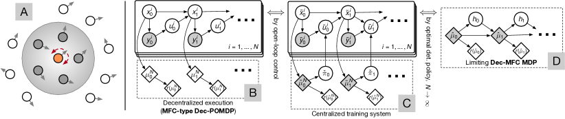
Figure 1: A: Partially-observable Vicsek problem: agents must align headings (arrows), but observe only partial information (e.g. heading distribution in grey circle for orange agent). B: The decentralized model as a graphical model (grey: observed variables). C: In centralized training, we also observe the mean field, guiding the learning of upper-level actions $\check{\pi}$. D: The solved limiting MDP.

Scalable and partially observable MARL.

Despite its many applications, decentralized cooperative control remains a difficult problem even in MARL [78], especially if coupled with the simultaneous requirement of scalability. Recent scalable state-of-the-art approaches include graphical decompositions [56, 77] and mean field control limits [12, 24, 42], amongst others [78]. However, a majority of approaches remains limited to full observability [77]. One recent line of scalable algorithms applies pairwise mean field approximations over neighbors on the value function [72], which has yielded some decentralized and partially observable extensions [21, 65]. In contrast, MARL algorithms based on mean field games (MFG, non-cooperative) and mean field control (MFC, cooperative) focus on a different, broad class of systems with many anonymously-interacting, permutation-invariant agents. While there are some theoretical results for the non-cooperative case in continuous-time [33, 62] and discrete-time [58], or e.g. for cooperative linear-quadratic models [67], to the best of our knowledge, neither MFC-based MARL algorithms nor discrete-time MFC have been proposed under partial information and decentralization. Beyond observability, MFGs (and not MFC) have been useful for analyzing emergence and collective behavior [51, 10], but less for "engineering" artificial collective behavior, as the aim of collective behavior is to achieve global objectives, which is contradicted (partially, e.g. [71, 36]) by egoistic agents, as decomposition of global objectives into per-agent rewards is non-trivial. Additionally, beyond scalability in number of agents, existing MFC learning still relies on discretization [12], which is not scalable to high-dimensional state-actions.

Our contribution.

A tractable framework for cooperative control, that can handle decentralized, partially observable systems, is missing. By the preceding motivation, we propose such a framework as illustrated in Figure 1. Our contributions may be summarized as (i) proposing the first discrete-time MFC model with decentralized and partially observable agents; (ii) providing accompanying theoretical foundations, including propagation of chaos, dynamic programming, and rigorous reformulations to a tractable single-agent Markov decision process (MDP); (iii) establishing a MARL algorithm with guarantees by the limiting background MDP; and (iv) presenting kernel-based MFC parametrizations of separate interest, to ensure requisite Lipschitz continuity, finer action control and general high-dimensional MFC. The algorithm is verified on various classical collective swarming behavior models, and compared against standard MARL. Overall, our framework provides tractable RL-based engineering of artificial collective behavior for large-scale multi-agent systems.

2 Decentralized Partially Observable MFC

In this section, we begin with introducing the motivating finite MFC-type decentralized partially observable control problem as a special case of cooperative, general decentralized partially observable Markov decision processes (Dec-POMDPs [6, 45]) to be solved. We then proceed to simplify in three steps of (i) taking the infinite-agent limit, (ii) relaxing partial observability, and (iii) weakening decentralization, in order to arrive at a tractable MDP with optimality guarantees, see also Figures 1 and 2. For readability, all proofs and implementation details are found in Appendices A–S.

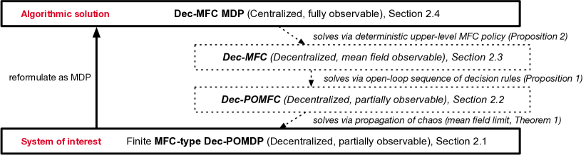
Figure 2: Three steps of approximation (mean field limit, open-loop control, and MDP reformulation) allow us to reformulate the broad class of MFC-type Dec-POMDP to a tractable Dec-MFC MDP.

2.1 MFC-type cooperative multi-agent control

To begin, we define the finite Dec-POMDP of interest, which is assumed of MFC-type. In other words, (i) agents are permutation invariant, i.e. only the overall distribution of agent states matters, and (ii) agents observe only part of the system. We assume agents $i\in[N]\coloneqq\{1,\ldots,N\}$ endowed with random states $x^{i}_{t}$, observations $y^{i}_{t}$ and actions $u^{i}_{t}$ at times $t\in\mathcal{T}\coloneqq\mathbb{N}$ from compact metric state, observation and action spaces $\mathcal{X}$, $\mathcal{Y}$, $\mathcal{U}$ (e.g. finite or continuous). Agent dynamics depend on other agents only via the empirical mean field (MF), i.e. the anonymous state distribution $\mu^{N}_{t}\coloneqq\frac{1}{N}\sum_{i\in[N]}\delta_{x^{i}_{t}}$ (full distribution, not only e.g. averages). Extending the MF to joint state-observation-action distributions is straightforward, but not expository. Policies are memory-less and shared by all agents, archetypal of collective behavior under simple rules [27], and of interest to compute-constrained agents, including e.g. nano-particles or small robots. Our model also allows limited memory by integration in the state, and analogously histories of observation-actions ("infinite" memory, see Appendix E). Agents act according to policy $\pi\in\Pi$ from a class $\Pi\subseteq\mathcal{P}(\mathcal{U})^{\mathcal{Y}\times\mathcal{T}}$ of policies, where $\mathcal{P}$ denotes spaces of probability measures metrized by the $1$-Wasserstein metric $W_{1}$ [70]. Starting with initial distribution $\mu_{0}$ and $x^{i}_{0}\sim\mu_{0}$, the MFC-type Dec-POMDP dynamics are

$$y^{i}_{t}\sim P^{y}(y^{i}_{t}\mid x^{i}_{t},\mu^{N}_{t}),\quad u^{i}_{t}\sim\pi_{t}(u^{i}_{t}\mid y^{i}_{t}),\quad x^{i}_{t+1}\sim P(x^{i}_{t+1}\mid x^{i}_{t},u^{i}_{t},\mu^{N}_{t})$$ (1)

for all $(i,t)\in[N]\times\mathcal{T}$, with transition kernels $P$, $P^{y}$, objective $J^{N}(\pi)=\operatorname{\mathbb{E}}[\sum_{t\in\mathcal{T}}\gamma^{t}r(\mu^{N}_{t})]$ to maximize over $\pi\in\Pi$, reward function $r\colon\mathcal{P}(\mathcal{X})\to\mathbb{R}$ and discount factor $\gamma\in(0,1)$. The theory also generalizes to finite horizons, and average per-agent rewards $r_{\mathrm{per}}\colon\mathcal{X}\to\mathbb{R}$ by $r(\mu^{N}_{t})=\int r_{\mathrm{per}}\mathrm{d}\mu^{N}_{t}$.

Since general Dec-POMDPs are hard [6], our model establishes a tractable special case of high generality. Standard MFC already covers a broad range of applications, e.g. see surveys for finance [9] and engineering [20] applications, which can now be handled under partial information. In addition, as mentioned in the introduction, many classical, inherently partially observable models are covered by MFC-type Dec-POMDPs, e.g. the Kuramoto or Vicsek models in Section 4, where similar ideas of MF limits and their convergence is referred to as propagation of chaos [13].

2.2 Limiting MFC system

In order to achieve tractability for large multi-agent systems, the first step is to take the infinite-agent limit. By a law of large numbers (LLN), this allows us to describe large systems only by the MF $\mu_{t}$. Consider a representative agent as in (1) with states $x_{0}\sim\mu_{0}$, $x_{t+1}\sim P(x_{t+1}\mid x_{t},u_{t},\mu_{t})$, observations $y_{t}\sim P^{y}(y_{t}\mid x_{t},\mu_{t})$ and actions $u_{t}\sim\pi_{t}(u_{t}\mid y_{t})$. Then, its state probability law replaces the empirical state distribution, informally $\mu_{t}=\mathcal{L}(x_{t})\equiv\lim_{N\to\infty}\mu^{N}_{t}$. Looking only at the MF, we obtain the decentralized partially observable MFC (Dec-POMFC) system via the prequel as

$$\mu_{t+1} =\mathcal{L}(x_{t+1})=T(\mu_{t},\pi_{t})\coloneqq\iiint P(x,u,\mu_{t})\pi_{t}(\mathrm{d}u\mid y)P^{y}(\mathrm{d}y\mid x,\mu_{t})\mu_{t}(\mathrm{d}x)$$ (2)

by deterministic transitions $T\colon\mathcal{P}(\mathcal{X})\times\mathcal{P}(\mathcal{U})^{\mathcal{Y}}\to\mathcal{P}(\mathcal{X})$ and objective $J(\pi)=\sum_{t=0}^{\infty}\gamma^{t}r(\mu_{t})$.

Propagation of chaos. Under mild continuity assumptions, the Dec-POMFC model in (2) constitutes a good approximation of large-scale MFC-type Dec-POMDP in (1) with many agents.

Assumption 1a.

The transition kernel $P\colon\mathcal{X}\times\mathcal{U}\times\mathcal{P}(\mathcal{X})\to\mathcal{P}(\mathcal{X})$ is $L_{P}$-Lipschitz continuous.

Assumption 1b.

The transition kernel $P^{y}\colon\mathcal{X}\times\mathcal{P}(\mathcal{X})\to\mathcal{P}(\mathcal{Y})$ is $L_{P^{y}}$-Lipschitz continuous.

Assumption 1c.

The reward function $r\colon\mathcal{P}(\mathcal{X})\to\mathbb{R}$ is $L_{r}$-Lipschitz continuous.

Assumption 1d.

The class of policies $\Pi$ for optimization is equi-Lipschitz, i.e. there exists $L_{\Pi}>0$ such that for all $t\in\mathcal{T}$ and $\pi\in\Pi$, $\pi_{t}\colon\mathcal{Y}\to\mathcal{P}(\mathcal{U})$ is $L_{\Pi}$-Lipschitz continuous.

In particular, Lipschitz continuity assumptions are standard [33, 24, 42] and for policies can result from neural networks (NNs) [50, 42] or appropriate parametrizations (Section 4). We obtain approximation guarantees similar to existing ones [24, 42, 16], but with additional partial observations.

Theorem 1.

Fix an equicontinuous family of functions $\mathcal{F}\subseteq\mathbb{R}^{\mathcal{P}(\mathcal{X})}$. Under Assumptions 1a, 1b, and 1d, the MF converges in the sense of $\sup_{\pi\in\Pi}\sup_{f\in\mathcal{F}}\operatorname{\mathbb{E}}\left[\left|f(\mu^{N}_{t})-f(\mu_{t})\right|\right]\to 0$ at all times $t\in\mathcal{T}$.

The above motivates the model, as it is now sufficient to find optimal $\pi$ not for the hard MFC-type Dec-POMDP, but instead for the possibly easier Dec-POMFC (which we will further simplify).

Corollary 1.

Under 1a–1d, any optimal Dec-POMFC policy $\pi\in\operatorname*{arg\,max}_{\pi^{\prime}\in\Pi}J(\pi^{\prime})$ is $\varepsilon$-optimal in the MFC-type Dec-POMDP, $J^{N}(\pi)\geq\sup_{\pi^{\prime}\in\Pi}J^{N}(\pi^{\prime})-\varepsilon$, with $\varepsilon\to 0$ as $N\to\infty$.

2.3 Mean field observability

Now impose observability of the MF (i.e. $\mu_{t}$ is $\sigma(y)$-measurable), and write policies as functions of both $y_{t}$ and $\mu_{t}$. The result is the decentralized mean field observable MFC (Dec-MFC) dynamics

$$\bar{\mu}_{t+1} =T(\bar{\mu}_{t},\bar{\pi}_{t}(\bar{\mu}_{t}))\coloneqq\iiint P(x,u,\mu_{t})\bar{\pi}_{t}(\mathrm{d}u\mid y,\bar{\mu}_{t})P^{y}(\mathrm{d}y\mid x,\bar{\mu}_{t})\bar{\mu}_{t}(\mathrm{d}x),$$ (3)

with shorthand $\bar{\pi}_{t}(\bar{\mu}_{t})=\bar{\pi}_{t}(\cdot\mid\cdot,\bar{\mu}_{t})$, initial $\bar{\mu}_{0}=\mu_{0}$ and according objective $\bar{J}(\bar{\pi})=\sum_{t=0}^{\infty}\gamma^{t}r(\bar{\mu}_{t})$ to optimize over (now MF-dependent) policies $\bar{\pi}\in\bar{\Pi}\subseteq\mathcal{P}(\mathcal{U})^{\mathcal{Y}\times\mathcal{P}(\mathcal{X})\times\mathcal{T}}$.

Rationale.

We provide three motivations for MF observability. First, agents may naturally observe the MF. Second, if the MF is unknown, a common approach to partially observable control is separation of filtering and control [3], by estimating the current MF. However, note that for multiple agents, there is no theoretical basis for separation. Therefore, the third, most compelling reason is that deterministic open-loop control transforms optimal Dec-MFC policies $\bar{\pi}\in\operatorname*{arg\,max}_{\bar{\pi}^{\prime}\in\bar{\Pi}}\bar{J}(\bar{\pi}^{\prime})$ into optimal Dec-POMFC policies $\pi\in\operatorname*{arg\,max}_{\pi\in\Pi}J(\pi)$ with decentralized execution, and vice versa: For given $\bar{\pi}$, compute deterministic MFs $(\bar{\mu}_{0},\bar{\mu}_{1},\ldots)$ via (3) and let $\pi=\Phi(\bar{\pi})$ by $\pi_{t}(\mathrm{d}u\mid y)=\bar{\pi}(\mathrm{d}u\mid y,\bar{\mu}_{t})$. Analogously, represent $\pi\in\Pi$ by $\bar{\pi}\in\bar{\Pi}$ with constant $\bar{\pi}_{t}(\nu)=\pi_{t}$ for all $\nu$.

Proposition 1.

For any $\bar{\pi}\in\bar{\Pi}$, define $(\bar{\mu}_{0},\bar{\mu}_{1},\ldots)$ as in (3). Then, for $\pi=\Phi(\bar{\pi})\in\Pi$, we have $\bar{J}(\bar{\pi})=J(\pi)$. Inversely, for any $\pi\in\Pi$, let $\bar{\pi}_{t}(\bar{\nu})=\pi_{t}$ for all $\bar{\nu}$, then again $\bar{J}(\bar{\pi})=J(\pi)$.

Corollary 2.

Optimal Dec-MFC policies $\bar{\pi}\in\operatorname*{arg\,max}_{\bar{\pi}^{\prime}\in\bar{\Pi}}\bar{J}(\bar{\pi}^{\prime})$ yield optimal Dec-POMFC policies $\Phi(\bar{\pi})$, i.e. $J(\Phi(\bar{\pi}))=\sup_{\pi^{\prime}\in\Pi}J(\pi^{\prime})$.

Hence, we may solve Dec-POMFC optimally by solving Dec-MFC. Knowing the initial distribution $\mu_{0}$ as in open-loop control is often realistic, as control is commonly deployed for a well-defined, given problem. Though even knowing $\mu_{0}$ is not strictly necessary for decentralized execution, see ablations in Section 4. Differences to standard open-loop control are that (i) each agent may have stochastic dynamics and observations, and (ii) agents randomize actions instead of precomputing. This is possible, as random agents still lead to quasi-deterministic MFs by the LLN. A last step is to reduce Dec-MFC with MF-dependent policies to an MDP with more tractable theory and algorithms.

2.4 Reduction to Dec-MFC MDP

The recent MFC MDP (or MFMDP, e.g. [54, 12, 23]) reformulates fully observable MFC as MDPs with higher-dimensional state-actions. Similarly, we find a reduction of Dec-MFC to a MDP with joint state-observation-action distributions as new MDP actions. We define the Dec-MFC MDP with states $\hat{\mu}_{t}\in\mathcal{P}(\mathcal{X})$ and actions $h_{t}\in\mathcal{H}(\hat{\mu}_{t})\subseteq\mathcal{P}(\mathcal{X}\times\mathcal{Y}\times\mathcal{U})$ from the set of desired joint distributions $h_{t}=\hat{\mu}_{t}\otimes P^{y}(\hat{\mu}_{t})\otimes\check{\pi}_{t}$ under a $L_{\Pi}$-Lipschitz decision rule $\check{\pi}_{t}\in\mathcal{P}(\mathcal{U})^{\mathcal{Y}}$. Here, $\nu\otimes K$ is the product measure of measure $\nu$ and kernel $K$, and $\nu K$ is the measure $\nu K=\int K(\cdot\mid x)\nu(\mathrm{d}x)$. For $\check{\pi}_{t}\in\mathcal{P}(\mathcal{U})^{\mathcal{Y}}$, $\mu_{xy}\in\mathcal{P}(\mathcal{X}\times\mathcal{Y})$, we write $\mu_{xy}\otimes\check{\pi}_{t}$ by considering $\check{\pi}_{t}$ constant on $\mathcal{X}$. In other words, the desired joint distribution $h_{t}$ results from all agents using lower-level decision rule $\check{\pi}_{t}$, which may be reobtained from $h_{t}$ a.e.-uniquely by disintegration [34]. The resulting dynamics are

$$h_{t}\sim\hat{\pi}(\hat{\mu}_{t}),\quad\hat{\mu}_{t+1}=\hat{T}(\hat{\mu}_{t},h_{t})\coloneqq\iiint P(x,u,\hat{\mu}_{t})h_{t}(\mathrm{d}x,\mathrm{d}y,\mathrm{d}u)$$ (4)

for upper-level MDP policy $\hat{\pi}\in\hat{\Pi}$ and objective $\hat{J}(\hat{\pi})=\operatorname{\mathbb{E}}\left[\sum_{t=0}^{\infty}\gamma^{t}r(\hat{\mu}_{t})\right]$. The MDP policy $\hat{\pi}$ is "upper-level", as we sample $h_{t}$ from $\hat{\pi}$, to then apply a lower-level decision rule $\check{\pi}_{t}$ to all agents.

Guidance by mean field observability.

The MF observation guides potentially hard decentralized problems, and allows reduction into a single-agent MDP where some existing theory can be made compatible. First, we formulate a dynamic programming principle (DPP), i.e. exact solutions by solving Bellman’s equation for the value function $V(\mu)=\sup_{h\in\mathcal{H}(\mu)}r(\mu)+\gamma V(\hat{T}(\mu,h))$ [29]. Simultaneously, we obtain sufficiency of stationary deterministic policies $\hat{\pi}$ for optimality. For technical reasons, only here we assume Hilbertian $\mathcal{Y}$ (e.g. finite, Euclidean & products) and finite $\mathcal{U}$.

Assumption 2.

The observations $\mathcal{Y}$ are a metric subspace of a Hilbert space. Actions $\mathcal{U}$ are finite.

Theorem 2.

Under 1a–1d and 2, there exists an optimal stationary, deterministic policy $\hat{\pi}$ for the Dec-MFC MDP, with $\hat{\pi}(\mu)\in\operatorname*{arg\,max}_{h\in\mathcal{H}(\mu)}r(\mu)+\gamma V(\hat{T}(\mu,h))$.

Decentralized execution without mean field observability.

Importantly, the guidance by the MF is required for training only, and not during decentralized execution. More precisely, an optimal MDP solution $\hat{\pi}\in\operatorname*{arg\,max}_{\hat{\pi}^{\prime}\in\hat{\Pi}}\hat{J}(\hat{\pi})$ yields optimal solutions also for the MFC-type Dec-POMDP with many agents, as long as $\hat{\pi}$ is deterministic (an optimal one exists by Theorem 2).

Proposition 2.

For deterministic $\hat{\pi}\in\hat{\Pi}$, let $\hat{\mu}_{t}$ as in (4) and $\bar{\pi}=\Psi(\hat{\pi})$ by $\bar{\pi}_{t}(\nu)=\check{\pi}_{t}$ for all $\nu$, then $\hat{J}(\hat{\pi})=\bar{J}(\bar{\pi})$. Inversely, for $\bar{\pi}\in\bar{\Pi}$, let $\hat{\pi}_{t}(\nu)=\nu\otimes P^{y}(\nu)\otimes\bar{\pi}_{t}(\nu)$ for all $\nu$, then $\hat{J}(\hat{\pi})=\bar{J}(\bar{\pi})$.

Note that the determinism of the upper-level policy is strictly necessary here. A simple counterexample is a problem where agents should choose to aggregate to one state. If the upper-level policy randomly chooses between moving all agents to either $A$ or $B$, then a random agent policy splits agents and fails to aggregate. At the same time, randomization of agent actions remains necessary for optimality, as the problem of equally spreading would require uniformly random agent actions.

Complexity of partially observable control.

Tractability of multi-agent control heavily depends on information structure [40]. General Dec-POMDPs have doubly-exponential complexity (NEXP) [6], and hence are significantly more complex than fully observable control (PSPACE, [47]). In contrast, Dec-POMFC surprisingly imposes little additional complexity over standard MFC, as the limiting model remains a deterministic MDP in the absence of common noise correlating agent states [11]. An extension to common noise is out of scope, as the key to our MDP reformulation is quasi-determinism by LLN, which is not given under (unknown, unpredictable) common noise.

3 Dec-POMFC Policy Gradient Methods

All that remains is to solve Dec-MFC MDPs. As we obtain continuous Dec-MFC MDP states and actions even for finite $\mathcal{X}$, $\mathcal{Y}$, $\mathcal{U}$, and infinite-dimensional ones for continuous $\mathcal{X}$, $\mathcal{Y}$, $\mathcal{U}$, a value-based approach can be hard, and we apply general policy-based RL. Our approach will allow finding simple decision rules for collective behavior, with emergence of global intelligent behavior described by rewards $r$, under arbitrary (Lipschitz) policies. For generality, we consider NN upper-level policies, with kernel representations for lower-level decision rules. While decision rules could also be parametrized by Lipschitz NNs [2] akin to hypernetworks [26], this yields distributions over NN parameters as MDP actions, which is too high-dimensional and failed in our experiments. Our MARL algorithm directly solves finite-agent MFC-type Dec-POMDPs by solving the Dec-MFC MDP in the background. Indeed, the theoretical optimality of Dec-MFC MDP solutions is guaranteed over Lipschitz policy classes $\Pi$ (and fulfilled by our novel kernel parametrizations in the following).

Corollary 3.

Under 1a–1d, a deterministic Dec-MFC solution $\hat{\pi}\in\operatorname*{arg\,max}_{\hat{\pi}^{\prime}}\hat{J}(\hat{\pi}^{\prime})$ is $\epsilon$-optimal in the Dec-POMDP with $\epsilon\to 0$ as $N\to\infty$, $J^{N}(\Phi(\Psi(\hat{\pi})))\geq\sup_{\pi^{\prime}\in\Pi}J^{N}(\pi^{\prime})-\epsilon$.

Histogram vs. kernel parametrizations.

To the best of our knowledge, the only existing approach to learning MFC in continuous spaces $\mathcal{X}\subseteq\mathbb{R}^{n}$, $n\in\mathbb{N}$ (and $\mathcal{Y}$ in our case) is by partitioning and "discretizing" [12]. Unfortunately, partitions fail Assumption 1d and therefore disallow optimality guarantees even for standard MFC. Instead, we propose kernel representations for both policy inputs (the MFs, for later gradient analysis), and Lipschitz lower-level decision rules $\check{\pi}_{t}$ for Assumption 1d.

In policy gradient methods with NNs, the MF state must be parametrized as input logits, while output logits constitute mean and log-standard deviation of a diagonal Gaussian over Lipschitz parameter representations $\xi\in\Xi$ of $\check{\pi}_{t}$. Specifically, as NN input, we let $\mathcal{P}(\mathcal{X})$-valued $\mu^{N}_{t}$ be represented not by the count of agents in each bin, but instead mollify around each center $x_{b}\in\mathcal{X}$ of $M_{\mathcal{X}}$ bins $b\in[M_{\mathcal{X}}]$ using kernels. The result is both Lipschitz and can approximate histograms well by Lipschitz partitions of unity [41, Theorem 1] over increasingly fine covers of the compact space $\mathcal{X}$. Hence, we obtain input logits $I_{b}=\int\kappa(x_{b},\cdot)\mathrm{d}\mu^{N}_{t}=\frac{1}{N}\sum_{i\in[N]}\kappa(x_{b},x^{i}_{t})$ for some kernel $\kappa\colon\mathcal{X}\times\mathcal{X}\to\mathbb{R}$ and $b\in[M_{\mathcal{X}}]$. Similarly, we obtain Lipschitz $\check{\pi}_{t}$ by representing $\check{\pi}_{t}$ via $M_{\mathcal{Y}}$ points $y_{b}\in\mathcal{Y}$ such that $\check{\pi}_{t}(u\mid y)=\sum_{b\in[M_{\mathcal{Y}}]}\kappa(y_{b},y)p_{b}(u)/\sum_{b\in[M_{\mathcal{Y}}]}\kappa(y_{b},y)$. Here, we consider $L_{\lambda}$-Lipschitz maps $\lambda$ from parameters $\xi\in\Xi$ to distributions $p_{b}=\lambda_{b}(\xi)\in\mathcal{P}(\mathcal{U})$ with compact parameter space $\Xi$, and for kernels choose RBF kernels $\kappa(x,y)=\exp(-\lVert x-y\rVert^{2}/(2\sigma^{2}))$ with some bandwidth $\sigma^{2}>0$.

Proposition 3.

Under RBF kernels $\kappa$, for any $\xi$ and continuous $\mathcal{Y}$, the decision rules $\Lambda(\xi)(\cdot\mid y)\coloneqq\sum_{b\in[M_{\mathcal{Y}}]}\kappa(y_{b},y)\lambda_{b}(\xi)/\sum_{b\in[M_{\mathcal{Y}}]}\kappa(y_{b},y)$ are $L_{\Pi}$-Lipschitz in $y$, as in Assumption 1d, if $\sigma^{2}\exp^{2}\left(-\frac{1}{2\sigma^{2}}\operatorname{diam}(\mathcal{Y})^{2}\right)\geq\frac{1}{L_{\Pi}}\operatorname{diam}(\mathcal{Y})\operatorname{diam}(\mathcal{U})\max_{y\in\mathcal{Y}}\lVert y\rVert$, and such $\sigma^{2}>0$ exists.

Proposition 3 ensures that Assumption 1d is fulfilled, and allows optimality guarantees by Corollary 3. In particular, deterministic policies are commonly achieved at convergence of stochastic policy gradients by taking action means, or can be guaranteed using deterministic policy gradients [63, 39].

Advantages of kernel representations for MFC.

Beyond their importance for (i) theoretical guarantees, and (ii) finer control over action distributions, another advantage is (iii) the improved complexity of kernel representations over histograms. Even a histogram with only $2$ bins per dimension needs $2^{d}$ bins in $d$-dimensional spaces, while kernel representations may place e.g. $2$ points per dimension, fixing the exponential complexity, as shown experimentally in Appendix A.

Direct multi-agent reinforcement learning algorithm.

Applying RL to the Dec-MFC MDP is satisfactory for solutions only under known MFC models. Our alternative direct MARL approach trains on a finite system of interest in a model-free manner. Importantly, we do not always have access to the model, and even if we do, it can be hard to parametrize MFs for arbitrary compact $\mathcal{X}$. Instead, it is both more practical and tractable to train on an $N$-agent MFC-type Dec-POMDP system. In order to exploit the underlying MDP, our algorithm must during training assume that (i) the MF is known, and (ii) agents can coordinate centrally. Therefore, the finite system (1) is adjusted for training by "correlating" agent actions on a single centrally sampled lower-level decision rule $\check{\pi}_{t}$. Now write $\hat{\pi}^{\theta}(\xi_{t}\mid\tilde{\mu}^{N}_{t})$ as density over parameters $\xi_{t}\in\Xi$ under a base measure (e.g. discrete, Lebesgue). Substituting $\xi_{t}$ as actions parametrizing $h_{t}$ in the MDP (4), e.g. by using RBF kernels, yields the centralized training system as seen in Figure 1 for stationary policy $\hat{\pi}^{\theta}$ parametrized by $\theta$,

$$\begin{split}\check{\pi}_{t}&=\Lambda(\tilde{\xi}_{t}),\quad\tilde{\xi}_{t}\sim\hat{\pi}^{\theta}(\tilde{\mu}^{N}_{t}),\\ \tilde{y}^{i}_{t}\sim P^{y}(\tilde{y}^{i}_{t}\mid\tilde{x}^{i}_{t},\tilde{\mu}^{N}_{t}),\quad\tilde{u}^{i}_{t}&\sim\check{\pi}_{t}(\tilde{u}^{i}_{t}\mid\tilde{y}^{i}_{t}),\quad\tilde{x}^{i}_{t+1}\sim P(\tilde{x}^{i}_{t+1}\mid\tilde{x}^{i}_{t},\tilde{u}^{i}_{t},\tilde{\mu}^{N}_{t}),\quad\forall i\in[N].\end{split}$$ (5)

Policy gradient approximation.

Since we train on a finite system, it is not immediately clear whether centralized training really yields the policy gradient for the underlying Dec-MFC MDP. We will show this fact up to an approximation. The general policy gradient for stationary $\hat{\pi}^{\theta}$ [66, 53] is

$$\nabla_{\theta}J(\hat{\pi}^{\theta})=(1-\gamma)^{-1}\operatorname{\mathbb{E}}_{\mu\sim d_{\hat{\pi}^{\theta}},\xi\sim\hat{\pi}^{\theta}(\mu)}\left[Q^{\theta}(\mu,\xi)\nabla_{\theta}\log\hat{\pi}^{\theta}(\xi\mid\mu)\right]$$

with $Q^{\theta}(\hat{\mu},\xi)=\operatorname{\mathbb{E}}[\sum_{t=0}^{\infty}\gamma^{t}r(\hat{\mu}_{t})\mid\hat{\mu}_{0}=\mu,\xi_{0}=\xi]$ in Dec-MFC MDP (4) using parametrized actions $\xi_{t}$, and the discounted sum $d_{\hat{\pi}^{\theta}}=(1-\gamma)\sum_{t\in\mathcal{T}}\gamma^{t}\mathcal{L}_{\hat{\pi}^{\theta}}(\hat{\mu}_{t})$ of laws of $\hat{\mu}_{t}$ under $\hat{\pi}^{\theta}$. Our approximation motivates MFC-based RL for MARL by showing that the underlying background Dec-MFC MDP is approximately solved under suitable Lipschitz parametrizations, e.g. we either normalize parameters $\xi$ to finite selected action’s probabilities, or diagonal Gaussian parameters.

Assumption 3.

The policy $\hat{\pi}^{\theta}(\xi\mid\mu)$ and its log-gradient $\nabla_{\theta}\log\hat{\pi}^{\theta}(\xi\mid\mu)$ are $L_{\hat{\Pi}}$, $L_{\nabla\hat{\Pi}}$-Lipschitz in $\mu$ and $\xi$ (or alternatively in $\mu$ for any $\xi$, and uniformly bounded). The parameter-to-distribution map is $\Lambda(\xi)(\cdot\mid y)\coloneqq\sum_{b}\kappa(y_{b},y)\lambda_{b}(\xi)(\cdot)/\sum_{b}\kappa(y_{b},y)$, with kernels $\kappa$ and $L_{\lambda}$-Lipschitz $\lambda_{b}\colon\Xi\to\mathcal{P}(\mathcal{U})$.

Theorem 3.

Centralized training on system (5) approximates the true gradient of the underlying Dec-MFC MDP, i.e. under RBF kernels $\kappa$ as in Proposition 3, 1a–1d and 3, as $N\to\infty$,

$$\left\|(1-\gamma)^{-1}\operatorname{\mathbb{E}}_{\mu\sim d^{N}_{\hat{\pi}^{\theta}},\xi\sim\hat{\pi}^{\theta}(\mu)}\left[\tilde{Q}^{\theta}(\mu,\xi)\nabla_{\theta}\log\hat{\pi}^{\theta}(\xi\mid\mu)\right]-\nabla_{\theta}J(\hat{\pi}^{\theta})\right\|\to 0$$

with $d^{N}_{\hat{\pi}^{\theta}}=(1-\gamma)\sum_{t\in\mathcal{T}}\gamma^{t}\mathcal{L}_{\hat{\pi}^{\theta}}(\tilde{\mu}^{N}_{t})$ and $\tilde{Q}^{\theta}(\mu,\xi)=\operatorname{\mathbb{E}}\left[\sum_{t=0}^{\infty}\gamma^{t}r(\tilde{\mu}^{N}_{t})\;\middle\lvert\;\mu_{0}=\mu,\xi_{0}=\xi\right]$.

The value function $\tilde{Q}^{\theta}$ in the finite system is then replaced in RL manner by on-policy and critic estimates. The Lipschitz conditions of $\hat{\pi}^{\theta}$ in Assumption 3 are fulfilled by Lipschitz NNs [50, 42, 2] and our aforementioned input parametrization. The approximation is novel, building a foundation for MARL via MFC directly on a finite system. Our results also apply to standard MFC by letting $y_{t}=x_{t}$. Though gradient estimates allow convergence guarantees in finite MDPs (e.g. [56, Theorem 5]), Dec-MFC MDP state-actions are always at least continuous, and theoretical analysis via discretization is out of scope. In practice, we use more efficient proximal policy optimization (PPO) [61] to obtain the decentralized partially observable mean field PPO algorithm (Dec-POMFPPO, Algorithm 1).

Algorithm 1 Dec-POMFPPO (during centralized training)

1:  for iteration $n=1,2,\ldots$ do

2:     for time $t=0,\ldots,B_{\mathrm{len}}-1$ do

3:        Sample central Dec-MFC MDP action $\check{\pi}_{t}=\Lambda(\xi_{t})$, $\xi_{t}\sim\hat{\pi}^{\theta}(\tilde{\mu}^{N}_{t})$.

4:        for agent $i=1,\ldots,N$ do

5:           Sample per-agent action $\tilde{u}^{i}_{t}\sim\check{\pi}_{t}(\tilde{u}^{i}_{t}\mid\tilde{y}^{i}_{t})$ for observation $\tilde{y}^{i}_{t}$.

6:        Perform actions, observe reward $r(\tilde{\mu}^{N}_{t})$, next MF $\tilde{\mu}^{N}_{t+1}$, termination flag $d_{t+1}\in\{0,1\}$.

7:     for updates $i=1,\ldots,N_{\mathrm{PPO}}$ do

8:        Sample mini-batch $b$, $|b|=b_{\mathrm{len}}$ from data $B\coloneqq((\tilde{\mu}^{N}_{t},\xi_{t},r^{N}_{t},d_{t+1},\tilde{\mu}^{N}_{t+1}))_{t\geq 0}$.

9:        Update policy $\hat{\pi}^{\theta}$ via the empirical PPO loss gradient $\nabla_{\theta}L_{\theta}$ on $b$, using GAE [60].

10:        Update critic $V^{\theta^{\prime}}$ via the empirical critic $L_{2}$-loss gradient $\nabla_{\theta^{\prime}}L_{\theta^{\prime}}$ on $b$.

Centralized training, decentralized execution.

Knowledge of the MF during training aligns our framework with the popular centralized training, decentralized execution (CTDE) paradigm. During training, the algorithm (i) assumes to observe the MF, and (ii) samples only one centralized $h_{t}$. By Theorem 3, we may learn directly on the MFC-type Dec-POMDP system (1). During execution, it suffices to execute decentralized policies for all agents without knowing the MF or coordinating centrally – as we have shown in Proposition 2 – with sufficiency for optimality by Corollary 3.

4 Numerical Evaluation

In this section, we present a numerical examination of our algorithm, comparing against independent PPO (IPPO), a MARL algorithm with consistent state-of-the-art performance [74, 48]. For comparison, we use the same implementation and hyperparameters for both IPPO and Dec-POMFPPO. For brevity, details of implementations, parameters, and more experiments are in Appendices A–C.

Problems.

In the simple Aggregation problem we consider a typical continuous single integrator model, commonly used in the study of swarm robotics [64, 4]. In the experiments, agents live in a box, observe their own position noisily and should aggregate. The classical Kuramoto model is used to study synchronization of coupled oscillators, finding application not only in physics, including quantum computation and laser arrays [1], but also in diverse biological systems, such as neuroscience and pattern formation in self-organizing systems [8, 35]. Its interdisciplinary reach highlights the model’s significance in understanding collective behavior in natural and artificial systems. Here, via partial observability, we consider a version where each oscillator can see the distribution of relative phases of its neighbors on a random geometric graph (e.g. [19]). In this work, we implement the Kuramoto model via omitting positions in its generalization, i.e. the well-known Vicsek model [68, 69]. Here, agents $i$ are described by their two-dimensional $[-1,1]^{2}$-valued position $p^{i}_{t}$ and current heading direction $\phi^{i}_{t}$, and may control their current heading by actions $u^{i}_{t}\in[u_{\mathrm{min}},u_{\mathrm{max}}]$, giving $p^{i}_{t+1}=p^{i}_{t}+v(\cos(\phi^{i}_{t}),\sin(\phi^{i}_{t}))$, $\phi^{i}_{t+1}=\phi^{i}_{t}+u^{i}_{t}+\epsilon^{i}_{t}$ for some Gaussian noise $\epsilon^{i}_{t}$ and velocity $v$. The key metric of interest for both the Kuramoto and Vicsek model is polarization, e.g. via the polar order parameter $R=\left|\frac{1}{N}\sum_{i}\exp\left(i\phi^{i}_{t}\right)\right|$ with the $i$-th agent’s phase $\phi^{i}_{t}$. The range of $R$ reaches from $0$, corresponding to a fully unsynchronized system, to $1$, resembling perfect alignment of all agents. Therefore, it is natural to use polarization-based objectives (with action costs) for the latter two models. Experimentally, we consider various environments via identifying $[-1,1]^{2}$ with 2D manifolds (including the regular torus, Möbius strip, projective plane and Klein bottle). In Vicsek, we allow control either via angular velocity, or also via additional forward velocity. Importantly, agents do not observe their own position or heading, but only relative headings of neighboring agents.

Training results.

In Figure 3 it is evident that the training process of MFC for many agents is relatively stable by guidance via MF and reduction to single-agent RL. In Appendix A, we also see similar results for training with significantly fewer agents. Surprisingly, even with a relatively small number of agents, the performance after training is already stable and comparable to the results obtained with a larger number of agents. This observation highlights that the training procedure yields satisfactory outcomes, even in scenarios where the mean field approximation may not yet be perfectly exact. These findings underscore the universality of the proposed approach and its ability to adapt across different regimes. On the same note, we see by comparison with Figure 4, that our method is usually on par with state-of-the-art IPPO MARL (comparing for many agents, $N=200$).

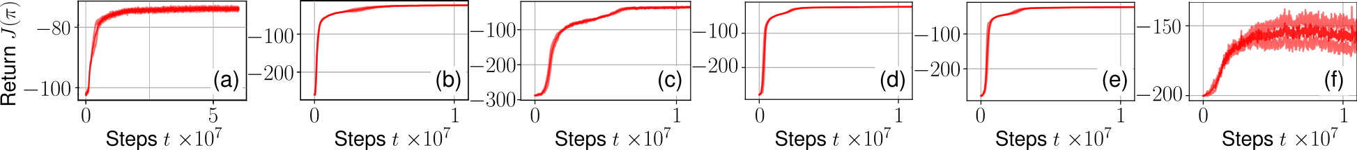
Figure 3: MFC training curves (episode return) with shaded standard deviation over $3$ seeds for $N=200$ in (a) Aggregation; Vicsek on a (b): torus; (c): Möbius strip; (d): projective plane; (e): Klein bottle; and (f) Kuramoto on a torus.

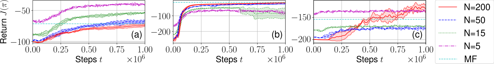
Figure 4: IPPO training curves (episode return) with shaded standard deviation over $3$ seeds and various $N$, in (a) Aggregation (box), (b) Vicsek (torus), (c) Kuramoto (torus). For comparison, we also plot the highest return averaged over $3$ seeds for Dec-POMFPPO in Figure 3 (MF, $N=200$).

Verification of theory.

Furthermore, we can see in Figure 5 that as the number of agents rises, the performance quickly tends to the limiting performance. In particular, the objective converges as the number of agents rises, supporting Theorem 1 and Corollary 1, as well as applicability to arbitrarily many agents. Analogously, conducting open-loop experiments on our closed-loop trained system as in Figure 6 demonstrates the robust generality and stability of the learned collective behavior with respect to the randomly sampled initial agent states, supporting Theorem 3 and Corollary 2.

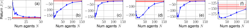
Figure 5: The performance of the best of $3$ final MFC policies transferred to $N$-agent systems (in blue), with error bars for $95\%$ confidence interval, averaged over $50$ episodes, and compared against the performance in the training system (in red). Problems (a)-(f) and training are as in Figure 3.

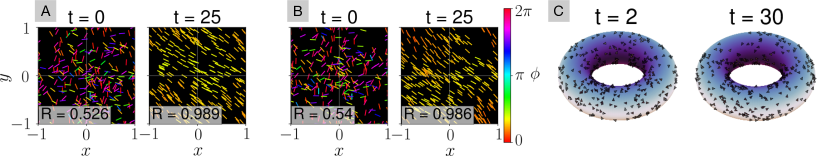
Figure 6: A, B: For the Vicsek (torus) problem with forward velocity control, the open-loop behavior (B) shows little difference in performance of agents (rods, color indicating heading) over the closed-loop behavior (A). C: Visualization of agents (triangles) under the Vicsek model on the torus.

Qualitative analysis.

In the Vicsek model, as seen exemplarily in Figure 6 and Appendix A, the algorithm learns to align in various topological spaces. In all considered topologies, the polar order parameter surpasses $0.9$, with the torus system even reaching a value close to $0.99$. As for the angles at different iterations of the training process, as depicted in Figure 7, the algorithm gradually learns to form a concentrated cluster of angles. Note that the cluster center angle is not fixed, but rather changes over time. This behavior can not be observed in the classical Vicsek model, though extensions using more sophisticated equations of motion for angles have reported similar results [35]. For more details and further experiments or visualizations, we refer the reader to Appendices A–C.

Figure 7 and additional figures, with similar results for other topologies in Appendix A, illustrate the qualitative behavior observed across the different manifolds. Agents on the continuous torus demonstrate no preference for a specific direction across consecutive training runs. Conversely, agents trained on other manifolds exhibit a tendency to avoid the direction that leads to an angle flip when crossing the corresponding boundary. Especially for the projective plane topology, the agents tend to aggregate more while aligning, even without adding another reward for aggregation. Another potential objective is misalignment in Figure 8, which can analogously be achieved, resulting in polar order parameters on the order of magnitude of $10^{-2}$, and showing the generality of the algorithm. In practice, one may set an arbitrary objective of interest. We analogously visualize the Aggregation problem in Figure 8, where we find successful aggregation of agents in the middle.

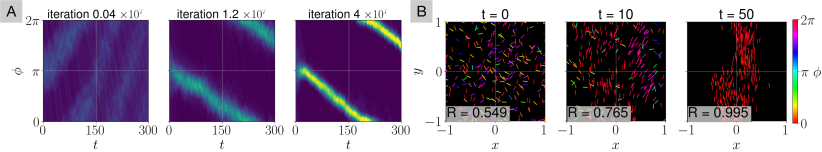
Figure 7: A: Agent angle alignment in the Vicsek model on the torus, plotted as density over time; B: Alignment of agents in the Vicsek model on the projective plane, as in Figure 6.

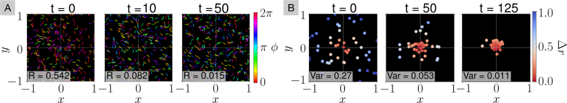
Figure 8: A: Qualitative behavior for misalignment of agents in the Vicsek (torus) problem. B: The two-dimensional Aggregation problem, with agent distances to mean as colors.

Additional experiments

Some other experiments are discussed in Appendix A, including the generalization of our learned policies to different starting conditions, a comparison of the Vicsek model trained or transferred to different numbers of agents, additional interpretative visualizations, also for the Kuramoto model, and a comparison between RBF and histogram parametrization, amongst other minor details, showing the generality of the approach or supporting theoretical claims.

5 Conclusion

Our framework provides a novel methodology for engineering artificial collective behavior in a mathematically founded and algorithmically tractable manner, whereas existing scalable learning frameworks often focus on competitive or fully observable models [25, 79]. We hope our work opens up new applications of partially-observable swarm systems. The current theory remains limited to non-stochastic MFs, which in the future could be analyzed for stochastic MFs via common noise [52, 16, 17]. Further, sample efficiency could be improved [32], and parametrizations for history-dependent decision rules using more general NNs could be considered, e.g. via hypernetworks [26, 37]. Lastly, extending the framework to consider additional practical constraints and sparser interactions, such as physical collisions or via graphical decompositions, may be fruitful.

Appendix A Additional Experiments

In this section, we give additional details on experiments. The mathematical description of problems can be found in Appendix C.

We use the manifolds as depicted in Figure 9 and as described in the following. Here, we visualize the qualitative results as in the main text for the remaining topologies. Due to technical limitations, all agents are drawn, including the ones behind a surface. To indicate where an agent belongs, we colorize the inside of the agent with the color of its corresponding surface.

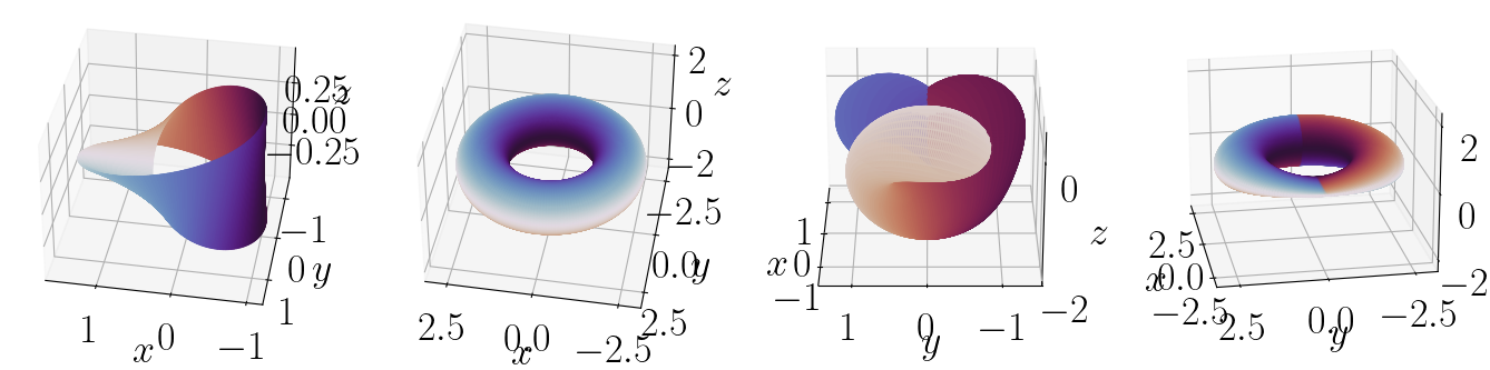
Figure 9: Two-dimensional manifolds visualized in three-dimensional space. In order from left to right: Möbius strip, torus, projective plane (Boy’s surface), and Klein bottle (pinched torus).

Torus manifold.

The (flat) torus manifold is obtained from the square $[-1,1]^{2}$ by identifying $(x,-1)\sim(x,1)$ and $(-1,y)\sim(1,y)$ for all $x,y\in[-1,1]$. For the metric, we use the toroidal distance inherited from the Euclidean distance $d_{2}$, which can be computed as

$$d(x,y)=\min_{t_{1},t_{2}\in\{-1,0,1\}}d_{2}(x,y+2t_{1}e_{1}+2t_{2}e_{2})$$

where $e_{1},e_{2}$ denote unit vectors. In Figure 9, we visualize the torus by mapping each point $(x,y)\in[-1,1]^{2}$ to a point $(X,Y,Z)$ in 3D space, given by

$$X =\left(2+0.75\cos\left(\pi(x+1)\right)\right)\cos\left(\pi(y+1)\right),$$

$$Y =\left(2+0.75\cos\left(\pi(x+1)\right)\right)\sin\left(\pi(y+1)\right),$$

$$Z =0.75\sin\left(\pi(x+1)\right).$$

The results have been described in the main text in Figure 7. Here, also note that the torus – by periodicity and periodic boundary conditions – can essentially be understood as the case of an infinite plane, consisting of infinitely many copies of the square $[-1,1]^{2}$ laid next to each other.

Möbius strip.

The Möbius strip is obtained from the square $[-1,1]^{2}$ by instead only identifying $(-1,-y)\sim(1,y)$ for all $y\in[-1,1]$, i.e. only the top and bottom side of the square, where directions are flipped. We then use the inherited distance

$$d(x,y)=\min_{t_{2}\in\{-1,0,1\}}d_{2}(x,(1-2\cdot\mathbf{1}_{t_{2}\neq 0},1)^{T}\odot y+2t_{2}e_{2})$$

where $\odot$ denotes the elementwise (Hadamard) product.

We visualize the Möbius strip in Figure 9 by mapping each point $(x,y)\in[-1,1]^{2}$ to

$$X =\left(1+\frac{x}{2}\cos\left(\frac{\pi}{2}(y+1)\right)\right)\cos\left(\pi(y+1)\right),$$

$$Y =\left(1+\frac{x}{2}\cos\left(\frac{\pi}{2}(y+1)\right)\right)\sin\left(\pi(y+1)\right),$$

$$Z =\frac{x}{2}\sin\left(\frac{\pi}{2}(y+1)\right).$$

As we can see in Figure 10, the behavior of agents is learned as expected: Agents learn to align along one direction on the Möbius strip.

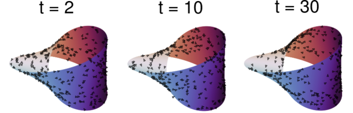
Figure 10: Qualitative visualization of Vicsek behavior on the Möbius strip manifold for uniform initialization. The $300$ agents (triangles) align into one direction on the Möbius strip.

Projective plane.

Analogously, the projective plane is obtained by identifying and flipping both sides of the square $[-1,1]^{2}$, i.e. $(-x,-1)\sim(x,1)$ and $(-1,-y)\sim(1,y)$ for all $x,y\in[-1,1]$. We use the inherited distance

$$d(x,y)=\min_{t_{1},t_{2}\in\{-1,0,1\}}d_{2}(x,(1-2\cdot\mathbf{1}_{t_{2}\neq 0},1-2\cdot\mathbf{1}_{t_{1}\neq 0})^{T}\odot y+2t_{1}e_{1}+2t_{2}e_{2})$$

and though an accurate visualization in less than four dimensions is difficult, we visualize in Figure 11 by mapping each point $(x,y)\in[-1,1]^{2}$ to a point $(X,Y,Z)$ on the so-called Boy’s surface, with

$$z =\frac{x+1}{2}\exp\left(i\pi(y+1)\right),$$

$$g_{1} =-\frac{3}{2}\operatorname{Im}\left(\frac{z(1-z^{4})}{z^{6}+\sqrt{5}z^{3}-1}\right),$$

$$g_{2} =-\frac{3}{2}\operatorname{Re}\left(\frac{z(1-z^{4})}{z^{6}+\sqrt{5}z^{3}-1}\right),$$

$$g_{3} =\operatorname{Im}\left(\frac{1+z^{6}}{z^{6}+\sqrt{5}z^{3}-1}\right)-\frac{1}{2},$$

$$X =\frac{g_{1}}{g_{1}^{2}+g_{2}^{2}+g_{3}^{2}},$$

$$Y =\frac{g_{2}}{g_{1}^{2}+g_{2}^{2}+g_{3}^{2}},$$

$$Z =\frac{g_{2}}{g_{1}^{2}+g_{2}^{2}+g_{3}^{2}}.$$

As we can see in Figure 11, under the inherited metric and radial parametrization, agents tend to gather at the bottom of the surface.

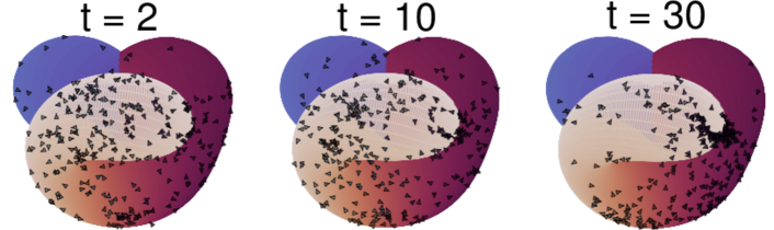
Figure 11: Qualitative visualization of Vicsek behavior on the projective plane manifold for uniform initialization. The $300$ agents (triangles) align over time by gathering at the bottom right.

Klein bottle.

Similarly, the Klein bottle is obtained by identifying both sides of the square $[-1,1]^{2}$ and flipping one side, i.e. $(x,-1)\sim(x,1)$ and $(-1,-y)\sim(1,y)$ for all $x,y\in[-1,1]$. We use the inherited distance

$$d(x,y)=\min_{t_{1},t_{2}\in\{-1,0,1\}}d_{2}(x,(1-2\cdot\mathbf{1}_{t_{2}\neq 0},1)^{T}\odot y+2t_{1}e_{1}+2t_{2}e_{2})$$

and visualize in Figure 12 by the pinched torus, i.e. mapping each $(x,y)\in[-1,1]^{2}$ to a point $(X,Y,Z)$ with

$$X =\left(2+0.75\cos\left(\pi(x+1)\right)\right)\cos\left(\pi(y+1)\right),$$

$$Y =\left(2+0.75\cos\left(\pi(x+1)\right)\right)\sin\left(\pi(y+1)\right),$$

$$Z =0.75\sin\left(\pi(x+1)\right))\cos\left(\frac{\pi}{2}(y+1)\right).$$

As we can see in Figure 12, agents may align by aggregating on the inner and outer ring, such that they may avoid switching sides at the pinch.

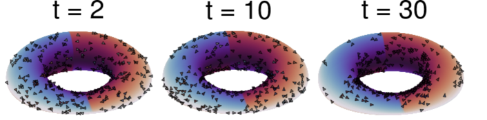
Figure 12: Qualitative visualization of behavior on Klein bottle topology for uniform initialization: The visualization in 3D is limited. Here, we use a pinched torus visualization that inverts itself at the flat pinch (i.e. there is no "connection" between blue and red surfaces at the bottom). Over time, $300$ agents (triangles) sometimes align by aggregating on the inner, avoiding side switches at the pinch.

Box.

Lastly, the box manifold is the square $[-1,1]^{2}$ equipped with the standard Euclidean topology, i.e. distances between two points $x,y\in[-1,1]^{2}$ are given by

$$d(x,y)=\sqrt{(x_{1}-y_{1})^{2}+(x_{2}-y_{2})^{2}},$$

while the sides of the square are not connected to anything else. We use the box manifold for the following experiments in Aggregation, and mention it here for sake of completeness.

Ablation on number of agents.

As seen in Figures 13 and  14, we can successfully train on various numbers of agents, despite the inaccuracy of the mean field approximation for fewer agents as inferred from Figure 5. This indicates that our algorithm is general and – at least in the considered problems – scales to arbitrary numbers of agents.

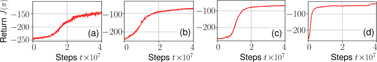
Figure 13: Training curves for Vicsek (torus), using RBF-based or discretization-based solutions. (a): RBF, $N=25$; (b): Discretization, $N=25$; (c): RBF, $N=50$; (d) : Discretization, $N=50$.

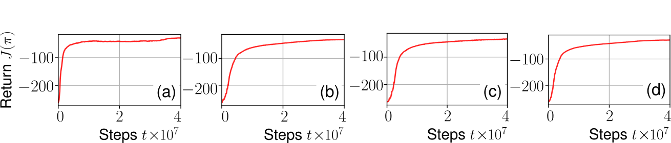
Figure 14: Training curves for Vicsek (torus), using RBF-based or discretization-based solutions. (a): RBF, $N=100$; (b): Discretization, $N=100$; (c): RBF, $N=150$; (d) : Discretization, $N=150$.

Qualitative results for Kuramoto.

The Kuramoto model, see Figure 15, demonstrates increased instability during training and subsequent lower-grade qualitative behavior compared to the Vicsek model. This disparity persists even when considering more intricate topologies, despite being a specialization of the Vicsek model. One explanation is that the added movement makes it easier to align agents over time. Another general explanation of non-alignment could be that, despite initially distributing agents uniformly across the region of interest, the learned policy causes the agents to aggregate into a few or even a single cluster (though we do not observe such behavior in Figure 15). The closer particles are to each other, the greater the likelihood that they perceive a similar or identical mean field, prompting alignment only in local clusters. A similar behavior is observed in the classical Vicsek model, where agents tend to move in the same direction after interaction. Consequently, they remain within each other’s interaction region and have the potential to form compounds provided there are no major disturbances. These can come from either other particles or excessively high levels of noise [5]. Although agents are able to align slightly, the desired alignment remains to be improved, either via more parameter tuning or improved algorithms.

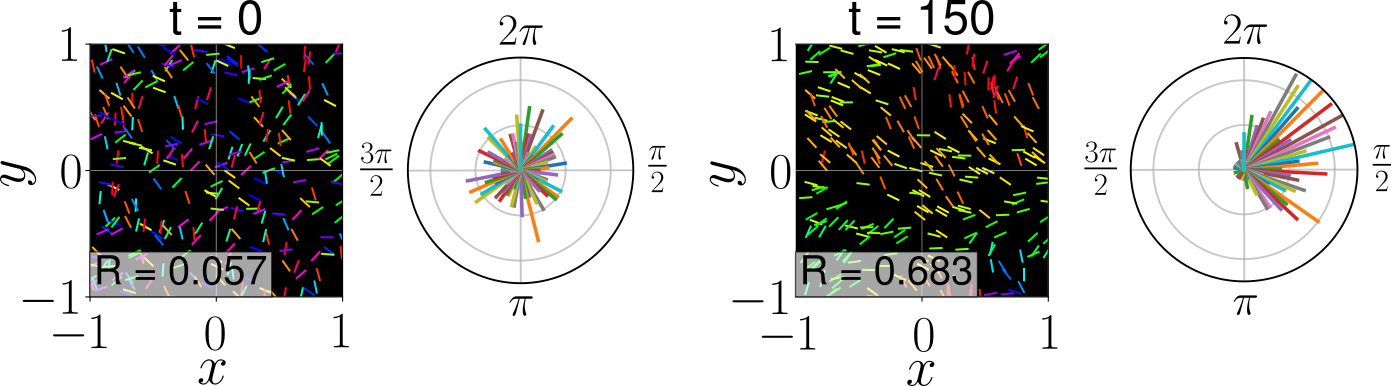
Figure 15: Qualitative behavior of the learned behavior in the Kuramoto model with histogram over angles, where in contrast to Vicsek, agents remain fixed in their initial position.

Effect of kernel method.

While for low dimensions, the effect of kernel methods is not as pronounced and mostly ensure theoretical guarantees, in Figures 16 and 17 we can see that training via our RBF-based methods outperforms discretization-based methods for dimensions higher than $3$ as compared to a simple gridding of the probability simplex with associated histogram representation of the mean field. Here, for the RBF method in Aggregation, we place $5$ equidistant points $y_{b}$ on the axis of each dimension. This is also the reason for why the discretization-based approach is better for low dimensions $d=2$ or $d=3$, as more points will have more control over actions of agents, and can therefore achieve better results, in exchange for tractability in high dimensions. This shows the advantage of RBF-based methods in more complex, high-dimensional problems. While the RBF-based method continues to learn even for higher dimensions up to $d=5$, the discretization-based solution eventually stops learning due to very large action spaces leading to increased noise on the gradient. The advantage is not just in terms of sample complexity, but also in terms of wall clock time, as the computation over exponentially many bins also takes more CPU time as shown in Table 1.

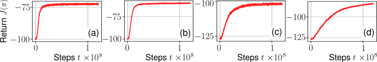
Figure 16: Training curves for $d$-dimensional Aggregation, using RBF-based or discretization-based solutions. (a): RBF, $d=2$; (b): Discretization, $d=2$; (c): RBF, $d=3$; (d) : Discretization, $d=3$.

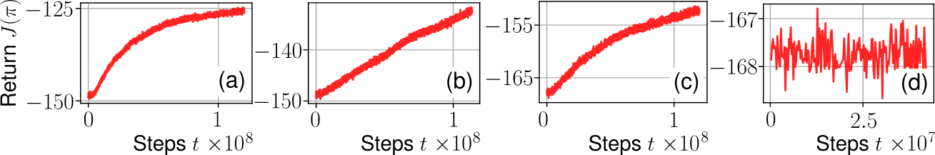
Figure 17: Training curves for $d$-dimensional Aggregation, using RBF-based or discretization-based solutions. (a): RBF, $d=4$; (b): Discretization, $d=4$; (c): RBF, $d=5$; (d) : Discretization, $d=5$.

Table 1: Wall clock time for one training step averaged over 3000 time steps in $d$-dimensional Aggregation.

Dimensionality $d$	RBF training time [s]	Discretization training time [s]
$2$	5.36	5.51
$3$	6.14	7.78
$4$	7.00	18.20
$5$	8.13	76.00

Ablations on time dependency and starting conditions.

As discussed in the main text, we also verify the effect of using a non-time-dependent open-loop sequence of lower-level policies, and also an ablation over different starting conditions. In particular, for starting conditions, to begin we will consider the uniform initialization as well as the beta-1, beta-2 and beta-3 initializations with a beta distribution over each dimension of the states, using $\alpha=\beta=0.5$, $\alpha=\beta=0.25$ and $\alpha=\beta=0.75$ respectively.

As we can see in Figure 18, the behavior learned for the Vicsek problem on the torus with $N=200$ agents allows for using the first lower-level policy $\check{\pi}_{0}$ at all times $t$ under the Gaussian initialization used in training to nonetheless achieve alignment. This validates the fact that a time-variant open-loop sequence of lower-level policies is not always needed, and the results even hold for slightly different initial conditions from the ones used in training.

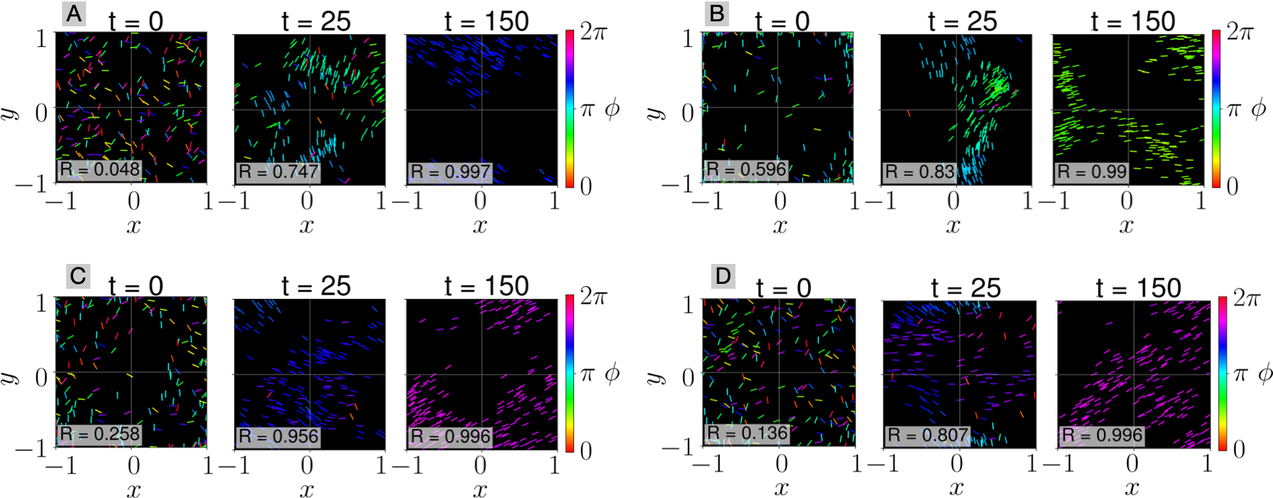
Figure 18: Open-loop behavior by using the lower-level decision policy at time $t=0$ for all times, on Vicsek (torus) with $N=200$ agents and various initializations. A: uniform initialization; B: beta-2 initialization; C: beta-1 initialization; D: beta-3 initialization.

Analogously, we consider some more strongly concentrated and heterogeneous initializations: The peak-normal initialization is given by a more concentrated zero-centered diagonal Gaussian with covariance $\sigma^{2}=0.1$. The squeezed-normal is the same initialization as in training, except for dividing the variance in the $y$-axis by $10$. The multiheaded-normal initialization is a mixture of two equisized Gaussian distributions in the upper-right and lower-left quadrant, where in comparison to the training initialization, position variances are halved. Finally, the bernoulli-multiheaded-normal additionally changes the weights of two Gaussians to $0.75$ and $0.25$ respectively.

As seen in Figure 19, the lower-level policy $\check{\pi}_{0}$ for Gaussian initialization from training easily transfers and generalizes to more complex initializations. However, the behavior may naturally be more suboptimal due to the training process likely never seeing more strongly concentrated and heterogeneous distributions of agents. For example, in the peak-normal initialization in Figure 19, we see that the agents begin relatively aligned, but will first misalign in order to align again, as the learned policy was trained to handle only the wider Gaussian initialization.

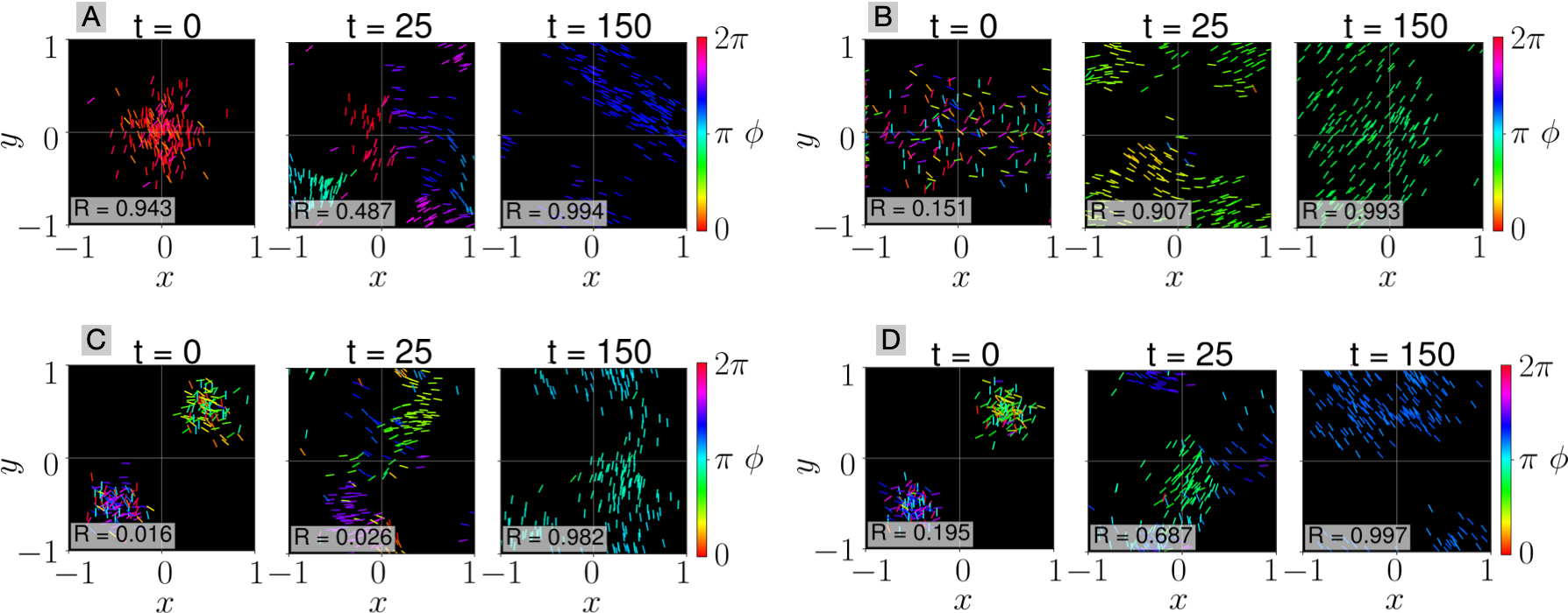
Figure 19: Open-loop behavior by using the lower-level decision policy at time $t=0$ for all times, on Vicsek (torus) with $N=200$ agents and various initializations. A: peak-normal initialization; B: squeezed-normal initialization; C: multiheaded-normal initialization; D: bernoulli-multiheaded-normal initialization.

No observations.

As an additional verification of the positive effect of mean field guidance on policy gradient training, we also perform experiments for training PPO without any RL observations, as in the previous paragraph we verified the applicability of learned behavior even without observing the MF that is observed by RL during training. In Figure 20 we see that PPO is unable to learn useful behavior, despite the existence of such a time-invariant lower-level policy from the preceding paragraph, underlining the empirical importance of mean field guidance that we derived.

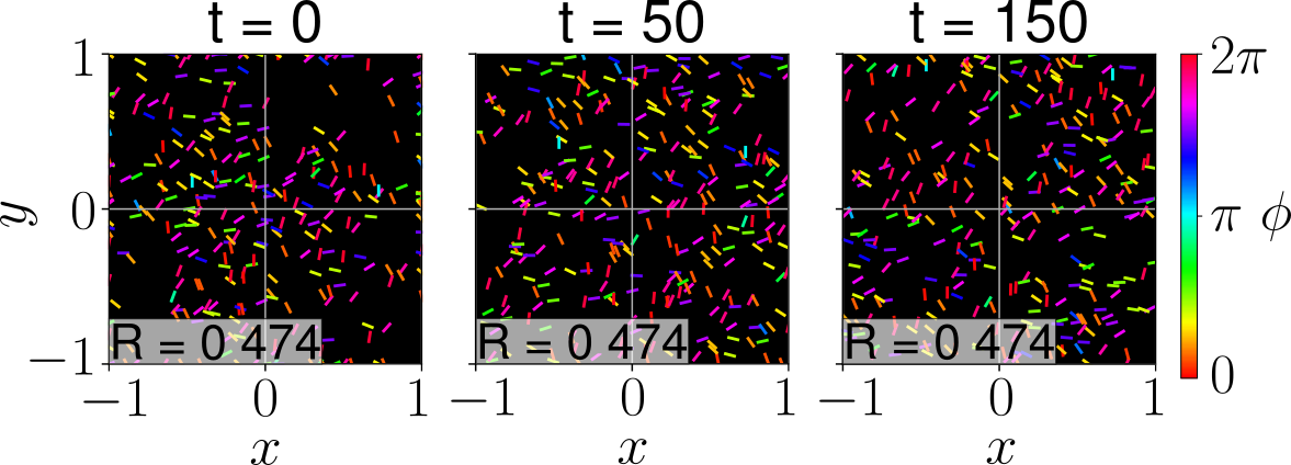
Figure 20: Qualitative behavior after training without observations for Vicsek (torus).

Transfer to differing agent counts.

In Figure 21, we see qualitatively that the behavior learned for $N=200$ agents transfers to different, lower numbers of agents as well. The result is congruent with the results shown in the main text, such as in Figure 5, and further supports the fact that our method scales to nearly arbitrary numbers of agents.

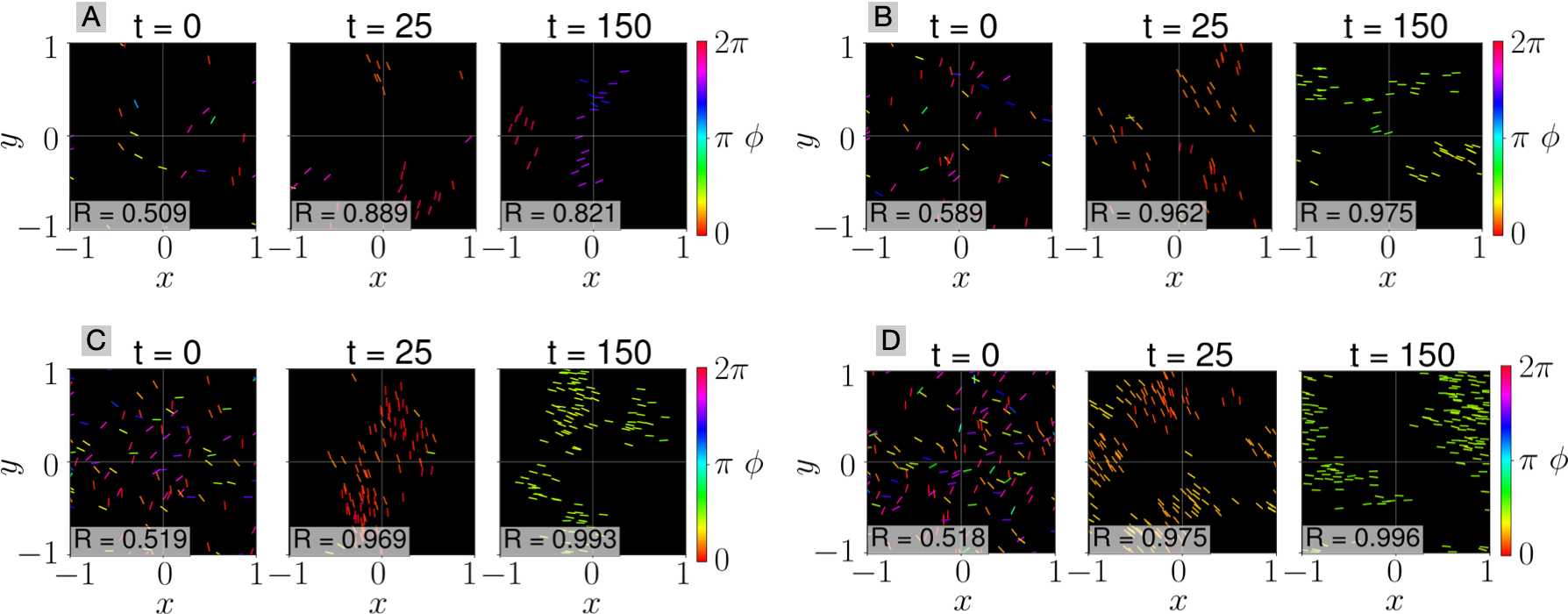
Figure 21: Qualitative behavior of the policy learned for $N=200$ on Vicsek (torus), transferred to different numbers of agents $N$. A: $N=25$; B: $N=50$; C: $N=100$; D: $N=150$.

Forward velocity control.

Lastly, we also allow agents to alternatively control their maximum velocity in the range $[0,v_{0}]$. Forward velocity can similarly be controlled, and allows for more uniform spreading of agents in contrast to the case where velocity cannot be controlled. This shows some additional generalization of our algorithm to variants of collective behavior problems. The corresponding final qualitative behavior is depicted in Figure 22.

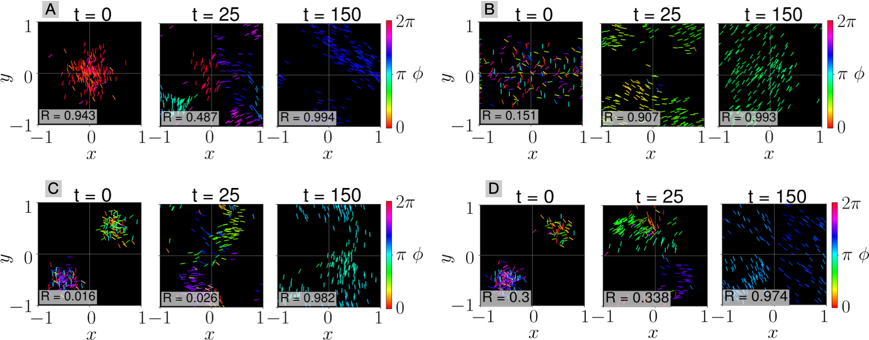
Figure 22: Qualitative behavior on Vicsek (torus) with $N=200$ agents, additional forward velocity control, and various initializations. A: peak-normal initialization; B: squeezed-normal initialization; C: multiheaded-normal initialization; D: bernoulli-multiheaded-normal initialization.

Appendix B Experimental Details

We use the RLlib $2.0.1$ (Apache-2.0 license) [38] implementation of PPO [61] for both MARL via IPPO, and our Dec-POMFPPO. For our experiments, we used no GPUs and around $60\,000$ Intel Xeon Platinum 9242 CPU core hours, and each training run usually took at most three days by training on at most $32$ CPU cores. Implementation-wise, for the upper-level policy NNs learned by PPO, we use two hidden layers with $256$ nodes and $\tanh$ activations, parametrizing diagonal Gaussians over the MDP actions $\xi\in\Xi$ (parametrizations of lower-level policies).

In Aggregation, we define the parameters $\xi\in\Xi$ for continuous spaces $\mathcal{X},\mathcal{Y},\mathcal{U}\subseteq\mathbb{R}^{d}$ by values in $\Xi\coloneqq[-1,1]^{2d}$. Each component of $\xi$ is then mapped affinely to mean in $\mathcal{U}$ or diagonal covariance in $[\epsilon,0.5+\epsilon]$ with $\epsilon=10^{-10}/4$, of each dimension. Meanwhile, in Vicsek and Kuramoto, we pursue a "discrete action space" approach, letting $\Xi\coloneqq[-1,1]^{3}$. We then affinely map components of $\xi\in\Xi$ to $[\epsilon,0.5+\epsilon]$, which are normalized to constitute probabilities of actions in $\{-1,0,1\}\subseteq\mathcal{U}$.

For the kernel-based representation of mean fields in $d$-dimensional state spaces $\mathcal{X}$, we define points $x_{b}$ by the center points of a $d$-dimensional gridding of spaces via equisized ($M_{\mathcal{X}}=5^{d}$ hypercubes) partitions. For the histogram, we similarly use the equisized hypercube partitions. For observation spaces $\mathcal{Y}$ and the kernel-based representation of lower-level policies, unless noted otherwise (e.g. in the high-dimensional experiments below, where we use less than exponentially many points), we do the same but additionally rescale the center points $\tilde{y}_{b}$ around zero, giving $y_{b}=c\tilde{y}_{b}$ for some $c>0$ and $M_{\mathcal{Y}}=5^{d}$. We use $c=0.75$ for Aggregation and $c=0.1$ for Vicsek and Kuramoto. For the (diagonal) bandwidths of RBF kernels, in Aggregation we use $\sigma=0.12/\sqrt{M_{\mathcal{X}}}$ for states and $\sigma=0.12c$ for observations. In Vicsek and Kuramoto, we use $\sigma=0.12/\sqrt{2}$ for state positions, $\sigma=0.12\pi$ for state angles, and $\sigma=0.06c$ or $\sigma=0.12\pi c$ for the first or second component of observations respectively. For IPPO, we observe the observations $y_{t}$ directly. For hyperparameters of PPO, see Table 2.

Table 2: PPO hyperparameter values.

Hyperparameter	Value
Discount factor $\gamma$	$0.99$
GAE lambda	$1$
KL coefficient	$0.03$
Clip parameter	$0.2$
Learning rate	$0.00005$
Training batch size $B_{\mathrm{len}}$	$4000$
Mini-batch size $b_{\mathrm{len}}$	$1000$
Steps per batch $N_{\mathrm{PPO}}$	$5$

Appendix C Problem Details

In this section, we will discuss in more detail the problems considered in our experiments.

Aggregation.

The Aggregation problem is a problem where agents must aggregate into a single point. Here, $\mathcal{X}=\mathcal{Y}=[-1,1]^{d}\subseteq\mathbb{R}^{d}$ for some dimensionality parameter $d\in\mathbb{N}$, and analogously $\mathcal{U}=[-1,1]^{d}$ for per-dimension movement actions. Observations are the own, noisily observed position, and movements are similarly noisy, using Gaussian noise. Overall, the dynamics are given by

$$y_{t} \sim\mathcal{N}\left(x_{t},\mathrm{diag}(\sigma^{2}_{y},\ldots\sigma^{2}_{y})\right),$$

$$x_{t+1} \sim\mathcal{N}\left(x_{t}+v_{0}\frac{u_{t}}{\max(1,\lVert u_{t}\rVert_{2})},\mathrm{diag}(\sigma^{2}_{x},\ldots\sigma^{2}_{x})\right)$$

for some velocity $v_{0}$, where additionally, observations and states that are outside of the box $[-1,1]^{d}$ are projected back to the box.

The reward function for aggregation of agents is defined as

$$r(\mu_{t})=-c_{d}\iint\lVert x-y\rVert_{1}\mu_{t}(\mathrm{d}x)\mu_{t}(\mathrm{d}y)-c_{u}\iint\left\lVert\frac{u}{\max(1,\lVert u\rVert_{2})}\right\rVert_{1}\pi_{t}(\mathrm{d}u\mid x)\mu_{t}(\mathrm{d}x),$$

for some disaggregation cost $c_{d}>0$ and action cost $c_{u}>0$, where we allow the dependence of rewards on actions as well: Note that our framework still applies to the above dependence on actions, as discussed in Section 2, by rewriting the system in the following way. At any even time $2t$, the agents transition from state $x\in\mathcal{X}$ to state-actions $(x,u)\in\mathcal{X}\times\mathcal{U}$, which will constitute the states of the new system. At the following odd times $2t+1$, the transition is sampled for the given state-actions. In this way, the mean field is over $\mathcal{X}\cup(\mathcal{X}\times\mathcal{U})$ and allows description of dependencies on the state-action distributions instead of only the state distribution.

For the experiments, we use $\sigma^{2}_{x}=0.04$, $\sigma^{2}_{y}=0.04$ and $v_{0}=0.1$. The initial distribution of agent positions is a Gaussian centered around zero, with variance $0.4$. The cost coefficients are $c_{d}=1$ and $c_{u}=0.1$. For simulation purposes, we consider episodes with length $T=100$.

Vicsek

In classical Vicsek models, each agent is coupled to every other agent within a predefined interaction region. The agents have a fixed maximum velocity $v_{0}>0$, and attempt to align themselves with the neighboring particles within their interaction range $D>0$. The equations governing the dynamics of the $i$-th agent in the classical Vicsek model are given in continuous time by

$$\mathrm{d}p^{i} =(v_{0}\sin(\phi^{i}),v_{0}\cos(\phi^{i}))^{T}\mathrm{d}t$$

$$\mathrm{d}\phi^{i} =\frac{1}{|N_{i}|}\sum_{j\in N_{i}}\sin\left(\phi^{j}-\phi^{i}\right)\mathrm{d}t+\sigma\mathrm{d}W$$

for all agents $i$, where $N_{i}$ denotes the set of agents within the interaction region, $N_{i}\coloneqq\{j\in[N]\mid d(x^{i},x^{j})\leq D\}$, and $W$ denotes Brownian motion.

We consider a discrete-time variant where agents may control independently how to adjust their angles in order to achieve a global objective (e.g. alignment, misalignment, aggregation). For states $x_{t}\equiv(p_{t},\phi_{t})$, actions $u_{t}$ and observations $y_{t}$, we have

$$(\bar{x},\bar{y})^{T} =\left(\iint\sin(\phi-\phi_{t})\mathbf{1}_{d(p_{t},p)\leq D}\mu_{t}(\mathrm{d}p,\mathrm{d}\phi),\iint\cos(\phi-\phi_{t})\mathbf{1}_{d(p_{t},p)\leq D}\mu_{t}(\mathrm{d}p,\mathrm{d}\phi)\right)^{T},$$

$$y_{t} =\left(\lVert(\bar{x},\bar{y})^{T}\rVert_{2},\operatorname{atan2}\left(\bar{x},\bar{y}\right)\right)^{T},$$

$$p_{t+1} =(p_{t,1}+v_{0}\sin(\phi_{t}),p_{t,2}+v_{0}\cos(\phi_{t}))^{T},$$

$$\phi_{t+1} \sim\mathcal{N}(\phi_{t}+\omega_{0}u_{t},\sigma_{\phi}^{2})$$

for some maximum angular velocity $\omega_{0}>0$ and noise covariance $\sigma_{\phi}^{2}>0$, where $\operatorname{atan2}(x,y)$ is the angle from the positive $x$-axis to the vector $(x,y)^{T}$. Therefore, we have $\mathcal{X}=[-1,1]^{2}\times[0,2\pi)$, where positions are equipped with the corresponding topologies discussed in Appendix A, and standard Euclidean spaces $\mathcal{Y}=[-1,1]^{2}$ and $\mathcal{U}=[-1,1]$. Importantly, agents only observe the relative headings of other agents within the interaction region. As a result, it is impossible to model such a system using standard MFC techniques.

As cost functions, we consider rewards via the polarization, plus action cost as in Aggregation. Defining polarization similarly to e.g. [75],

$$\mathrm{pol}_{t} \coloneqq\iint\angle(x,\bar{x}_{t})\mu_{t}(\mathrm{d}p,\mathrm{d}\phi),$$

$$\angle(x,y) \coloneqq\arccos\left((\cos(\phi),\sin(\phi))^{T}\cdot\frac{y}{\lVert y\rVert_{2}}\right),$$

$$\bar{x}_{t} \coloneqq\iint(\cos(\phi),\sin(\phi))^{T}\mu_{t}(\mathrm{d}p,\mathrm{d}\phi)$$

where high values of $\mathrm{pol}_{t}$ indicate misalignment, we define the rewards for alignment

$$r(\mu_{t})=-c_{a}\mathrm{pol}_{t}-c_{u}\iint|u|\pi_{t}(\mathrm{d}u\mid x)\mu_{t}(\mathrm{d}x),$$

and analogously for misalignment

$$r(\mu_{t})=+c_{a}\mathrm{pol}_{t}-c_{u}\iint|u|\pi_{t}(\mathrm{d}u\mid x)\mu_{t}(\mathrm{d}x).$$

For our training, unless noted otherwise, we let $D=0.25$, $v_{0}=0.075$, $\omega_{0}=0.2$, $\sigma_{\phi}=0.02$ and $\mu_{0}$ as a zero-centered (clipped) diagonal Gaussian with variance $0.4$. The cost coefficients are $c_{a}=1$ and $c_{u}=0.1$. For simulation purposes, we consider episodes with length $T=200$.

Kuramoto.

The Kuramoto model can be obtained from the Vicsek model by setting the maximal velocity $v_{0}$ of the above equations to zero. Hence, we obtain a random geometric graph, where agents see only their neighbor’s state distribution within the interaction region, and the neighbors are static per episode. For parameters, we let $D=0.25$, $v_{0}=0$, $\omega_{0}=0.2$, $\sigma_{\phi}=0$ and $\mu_{0}$ as a zero-centered (clipped) Gaussian with variance $0.4$. The cost coefficients are $c_{a}=1$ and $c_{u}=0.1$. For simulation purposes, we consider episodes with length $T=200$.

Appendix D Propagation of Chaos

Proof of Theorem 1.

As in the main text, we usually equip $\mathcal{P}(\mathcal{X})$ with the $1$-Wasserstein distance. In the proof, however, it is useful to also consider the uniformly equivalent metric $d_{\Sigma}(\mu,\mu^{\prime})\coloneqq\sum_{m=1}^{\infty}2^{-m}|\int f_{m}\,\mathrm{d}(\mu-\mu^{\prime})|$ instead. Here, $(f_{m})_{m\geq 1}$ is a fixed sequence of continuous functions $f_{m}\colon\mathcal{X}\to[-1,1]$, see e.g. [49, Theorem 6.6] for details.

First, let us define the measure $\zeta^{\pi,\mu}_{t}$ on $\mathcal{X}\times\mathcal{U}$, defined for any measurable set $A\times B\subseteq\mathcal{X}\times\mathcal{U}$ by $\zeta^{\pi,\mu}_{t}(A\times B)\coloneqq\int_{A}\int_{\mathcal{Y}}\int_{B}\pi_{t}(\mathrm{d}u\mid y)P^{y}(\mathrm{d}y\mid x,\mu_{t})\mu_{t}(\mathrm{d}x)$. For notational convenience we define the MF transition operator $\tilde{T}$ such that

$$\tilde{T}(\mu_{t},\zeta^{\pi,\mu}_{t}) \coloneqq\iint P(\cdot\mid x,u,\mu_{t})\zeta^{\pi,\mu}_{t}(\mathrm{d}x,\mathrm{d}u)=\mu_{t+1}.$$ (6)

Continuity of $\tilde{T}$ follows immediately from Assumption 1a and [16, Lemma 2.5] which we recall here for convenience.

Proposition 4 ([16], Lemma 2.5).

Under Assumption 1a, $(\mu_{n},\zeta_{n})\to(\mu,\zeta)$ implies $\tilde{T}(\mu_{n},\zeta_{n})\to\tilde{T}(\mu,\zeta)$.

The rest of the proof is similar to [16, Theorem 2.7] – though we remark that we strengthen the convergence statement from weak convergence to convergence in $L_{1}$ uniformly over $f\in\mathcal{F}$ – by showing via induction over $t$ that

$$\sup_{\pi\in\Pi}\sup_{f\in\mathcal{F}}\operatorname{\mathbb{E}}\left[\left|f(\mu^{N}_{t})-f(\mu_{t})\right|\right]\to 0.$$ (7)

Note that the induction start can be verified by a weak LLN argument which is also leveraged in the subsequent induction step. For the induction step we assume that (7) holds at time $t$. At time $t+1$ we have

$$\sup_{\pi\in\Pi}\sup_{f\in\mathcal{F}}\operatorname{\mathbb{E}}\left[\left|f(\mu^{N}_{t+1})-f(\mu_{t+1})\right|\right]$$

$$\quad\leq\sup_{\pi\in\Pi}\sup_{f\in\mathcal{F}}\operatorname{\mathbb{E}}\left[\left|f(\mu^{N}_{t+1})-f\left(\tilde{T}\left(\mu^{N}_{t},\zeta^{\pi,\mu^{N}}_{t}\right)\right)\right|\right]$$ (8)

$$\qquad+\sup_{\pi\in\Pi}\sup_{f\in\mathcal{F}}\operatorname{\mathbb{E}}\left[\left|f\left(\tilde{T}\left(\mu^{N}_{t},\zeta^{\pi,\mu^{N}}_{t}\right)\right)-f(\mu_{t+1})\right|\right].$$ (9)

We start by analyzing the first term and recall that a modulus of continuity $\omega_{\mathcal{F}}$ of $\mathcal{F}$ is defined as a function $\omega_{\mathcal{F}}\colon[0,\infty)\to[0,\infty)$ with both $\lim_{x\to 0}\omega_{\mathcal{F}}(x)=0$ and $|f(\mu)-f(\nu)|\leq\omega_{\mathcal{F}}(W_{1}(\mu,\nu)),\forall f\in\mathcal{F}$. By [18, Lemma 6.1], such a non-concave and decreasing modulus $\omega_{\mathcal{F}}$ exists for $\mathcal{F}$ because it is uniformly equicontinuous due to the compactness of $\mathcal{P}(\mathcal{X})$. Analogously, we have that $\mathcal{F}$ is uniformly equicontinuous in the space $(\mathcal{P}(\mathcal{X}),d_{\Sigma})$ as well. Recalling that $\mathcal{P}(\mathcal{X})$ is compact and the topology of weak convergence is metrized by both $d_{\Sigma}$ and $W_{1}$, we know that the identity map $\mathrm{id}\colon(\mathcal{P}(\mathcal{X}),d_{\Sigma})\to(\mathcal{P}(\mathcal{X}),W_{1})$ is uniformly continuous. Leveraging the above findings, we have that for the identity map there exists a modulus of continuity $\tilde{\omega}$ such that

$$|f(\mu)-f(\nu)|\leq\omega_{\mathcal{F}}(W_{1}(\mathrm{id}\,\mu,\mathrm{id}\,\nu))\leq\omega_{\mathcal{F}}(\tilde{\omega}(d_{\Sigma}(\mu,\nu)))$$

holds for all $\mu,\nu\in(\mathcal{P}(\mathcal{X}),d_{\Sigma})$. By [18, Lemma 6.1], we can use the least concave majorant of $\tilde{\omega}_{\mathcal{F}}\coloneqq\omega_{\mathcal{F}}\circ\tilde{\omega}$ instead of $\tilde{\omega}_{\mathcal{F}}$ itself. Then, (8) can be bounded by

$$\operatorname{\mathbb{E}}\left[\left|f(\mu^{N}_{t+1})-f\left(\tilde{T}\left(\mu^{N}_{t},\zeta^{\pi,\mu^{N}}_{t}\right)\right)\right|\right] \leq\operatorname{\mathbb{E}}\left[\tilde{\omega}_{\mathcal{F}}\left(d_{\Sigma}\left(\mu^{N}_{t+1},\tilde{T}\left(\mu^{N}_{t},\zeta^{\pi,\mu^{N}}_{t}\right)\right)\right)\right]$$

$$\leq\tilde{\omega}_{\mathcal{F}}\left(\operatorname{\mathbb{E}}\left[d_{\Sigma}\left(\mu^{N}_{t+1},\tilde{T}\left(\mu^{N}_{t},\zeta^{\pi,\mu^{N}}_{t}\right)\right)\right]\right)$$

irrespective of both $\pi$ and $f$ by the concavity of $\tilde{\omega}_{\mathcal{F}}$ and Jensen’s inequality. For notational convenience, we define $x^{N}_{t}\coloneqq(x^{i,N}_{t})_{i\in[N]}$, and arrive at

$$\operatorname{\mathbb{E}}\left[d_{\Sigma}\left(\mu^{N}_{t+1},\tilde{T}\left(\mu^{N}_{t},\zeta^{\pi,\mu^{N}}_{t}\right)\right)\right] =\sum_{m=1}^{\infty}2^{-m}\operatorname{\mathbb{E}}\left[\left|\int f_{m}\,\mathrm{d}\left(\mu^{N}_{t+1}-\tilde{T}\left(\mu^{N}_{t},\zeta^{\pi,\mu^{N}}_{t}\right)\right)\right|\right]$$

$$\leq\sup_{m\geq 1}\operatorname{\mathbb{E}}\left[\operatorname{\mathbb{E}}\left[\left|\int f_{m}\,\mathrm{d}\left(\mu^{N}_{t+1}-\tilde{T}\left(\mu^{N}_{t},\zeta^{\pi,\mu^{N}}_{t}\right)\right)\right|\;\middle\lvert\;x^{N}_{t}\right]\right].$$

Finally, we require the aforementioned weak LLN argument which goes as follows

$$\operatorname{\mathbb{E}}\left[\left|\int f_{m}\,\mathrm{d}\left(\mu^{N}_{t+1}-\tilde{T}\left(\mu^{N}_{t},\zeta^{\pi,\mu^{N}}_{t}\right)\right)\right|\;\middle\lvert\;x^{N}_{t}\right]^{2}$$

$$\quad=\operatorname{\mathbb{E}}\left[\left|\frac{1}{N}\sum_{i\in[N]}\left(f_{m}(x^{i}_{t+1})-\operatorname{\mathbb{E}}\left[f_{m}(x^{i}_{t+1})\;\middle\lvert\;x^{N}_{t}\right]\right)\right|\;\middle\lvert\;x^{N}_{t}\right]^{2}$$

$$\quad\leq\operatorname{\mathbb{E}}\left[\left|\frac{1}{N}\sum_{i\in[N]}\left(f_{m}(x^{i}_{t+1})-\operatorname{\mathbb{E}}\left[f_{m}(x^{i}_{t+1})\;\middle\lvert\;x^{N}_{t}\right]\right)\right|^{2}\;\middle\lvert\;x^{N}_{t}\right]$$

$$\quad=\frac{1}{N^{2}}\sum_{i\in[N]}\operatorname{\mathbb{E}}\left[\left(f_{m}(x^{i}_{t+1})-\operatorname{\mathbb{E}}\left[f_{m}(x^{i}_{t+1})\;\middle\lvert\;x^{N}_{t}\right]\right)^{2}\;\middle\lvert\;x^{N}_{t}\right]\leq\frac{4}{N}\to 0.$$

Here, we have used that $|f_{m}|\leq 1$, as well as the conditional independence of $x^{i}_{t+1}$ given $x^{N}_{t}$. In combination with the above results, the term (8) thus converges to zero. Moving on to the remaining second term (9), we note that the induction assumption implies that

$$\sup_{\pi\in\Pi}\sup_{f\in\mathcal{F}}\operatorname{\mathbb{E}}\left[\left|f\left(\tilde{T}\left(\mu^{N}_{t},\zeta^{\pi,\mu^{N}}_{t}\right)\right)-f(\mu_{t+1})\right|\right]$$

$$\quad=\sup_{\pi\in\Pi}\sup_{f\in\mathcal{F}}\operatorname{\mathbb{E}}\left[\left|f\left(\tilde{T}\left(\mu^{N}_{t},\zeta^{\pi,\mu^{N}}_{t}\right)\right)-f\left(\tilde{T}\left(\mu_{t},\zeta^{\pi,\mu}_{t}\right)\right)\right|\right]$$

$$\quad\leq\sup_{\pi\in\Pi}\sup_{g\in\mathcal{G}}\operatorname{\mathbb{E}}\left[\left|g(\mu^{N}_{t})-g(\mu_{t})\right|\right]\to 0$$

using the function $g\coloneqq f\circ\tilde{T}^{\pi_{t}}_{*}$ which belongs to the class $\mathcal{G}$ of equicontinuous functions with modulus of continuity $\omega_{\mathcal{G}}\coloneqq\omega_{\mathcal{F}}\circ\omega_{\tilde{T}}$. Here, $\omega_{\tilde{T}}$ is the uniform modulus of continuity over all policies $\pi$ of $\mu_{t}\mapsto\tilde{T}^{\pi_{t}}_{*}(\mu_{t})\coloneqq\tilde{T}(\mu_{t},\zeta^{\pi,\mu}_{t})$. The equicontinuity of $\{\tilde{T}^{\pi_{t}}_{*}\}_{\pi\in\Pi}$ is a consequence of Lemma 4 as well as the equicontinuity of functions $\mu_{t}\mapsto\zeta^{\pi,\mu}_{t}$ which in turn follows from the uniform Lipschitzness of $\Pi$. The validation of this claim is provided in the next lines. Note that this also completes the induction and thereby the proof. For a sequence of $\mu_{n}\to\mu\in\mathcal{P}(\mathcal{X})$ we can write

$$\sup_{\pi\in\Pi}W_{1}(\zeta^{\pi,\mu_{n}}_{t},\zeta^{\pi,\mu}_{t})$$

$$\qquad\leq\sup_{\pi\in\Pi}\sup_{\lVert f^{\prime}\rVert_{\mathrm{Lip}}\leq 1}\left|\iiint f^{\prime}(x,u)\pi_{t}(\mathrm{d}u\mid y)(P^{y}(\mathrm{d}y\mid x,\mu_{n})-P^{y}(\mathrm{d}y\mid x,\mu))\mu_{n}(\mathrm{d}x)\right|$$

$$\qquad\quad+\sup_{\pi\in\Pi}\sup_{\lVert f^{\prime}\rVert_{\mathrm{Lip}}\leq 1}\left|\iiint f^{\prime}(x,u)\pi_{t}(\mathrm{d}u\mid y)P^{y}(\mathrm{d}y\mid x,\mu)(\mu_{n}(\mathrm{d}x)-\mu(\mathrm{d}x))\right|.$$

Starting with the first term, we apply Assumptions 1b and 1d to arrive at

$$\sup_{\pi\in\Pi}\sup_{\lVert f^{\prime}\rVert_{\mathrm{Lip}}\leq 1}\left|\iiint f^{\prime}(x,u)\pi_{t}(\mathrm{d}u\mid y)(P^{y}(\mathrm{d}y\mid x,\mu_{n})-P^{y}(\mathrm{d}y\mid x,\mu))\mu_{n}(\mathrm{d}x)\right|$$

$$\quad\leq\sup_{\pi\in\Pi}\sup_{\lVert f^{\prime}\rVert_{\mathrm{Lip}}\leq 1}\int\left|\iint f^{\prime}(x,u)\pi_{t}(\mathrm{d}u\mid y)(P^{y}(\mathrm{d}y\mid x,\mu_{n})-P^{y}(\mathrm{d}y\mid x,\mu))\right|\mu_{n}(\mathrm{d}x)$$

$$\quad\leq\sup_{\pi\in\Pi}\sup_{\lVert f^{\prime}\rVert_{\mathrm{Lip}}\leq 1}\sup_{x\in\mathcal{X}}\left|\iint f^{\prime}(x,u)\pi_{t}(\mathrm{d}u\mid y)(P^{y}(\mathrm{d}y\mid x,\mu_{n})-P^{y}(\mathrm{d}y\mid x,\mu))\right|$$

$$\quad\leq L_{\Pi}\sup_{x\in\mathcal{X}}W_{1}(P^{y}(\cdot\mid x,\mu_{n}),P^{y}(\cdot\mid x,\mu))$$

$$\quad\leq L_{\Pi}L_{P^{y}}W_{1}(\mu_{n},\mu)\to 0$$

with Lipschitz constant $L_{\Pi}$ corresponding to the Lipschitz function $y\mapsto\int f^{\prime}(x,u)\pi_{t}(\mathrm{d}u\mid y)$. In a similar fashion, we point out the $1$-Lipschitzness of $x\mapsto\iint\frac{f^{\prime}(x,u)}{L_{\Pi}L_{P^{y}}+1}\pi_{t}(\mathrm{d}u\mid y)P^{y}(\mathrm{d}y\mid x,\mu)$, as

$$\left|\iint\frac{f^{\prime}(z,u)}{L_{\Pi}L_{P^{y}}+1}\pi_{t}(\mathrm{d}u\mid y)P^{y}(\mathrm{d}y\mid z,\mu)-\iint\frac{f^{\prime}(x,u)}{L_{\Pi}L_{P^{y}}+1}\pi_{t}(\mathrm{d}u\mid y)P^{y}(\mathrm{d}y\mid x,\mu)\right|$$

$$\quad\leq\left|\iint\frac{f^{\prime}(z,u)-f^{\prime}(x,u)}{L_{\Pi}L_{P^{y}}+1}\pi_{t}(\mathrm{d}u\mid y)P^{y}(\mathrm{d}y\mid z,\mu)\right|$$

$$\qquad+\left|\iint\frac{f^{\prime}(x,u)}{L_{\Pi}L_{P^{y}}+1}\pi_{t}(\mathrm{d}u\mid y)(P^{y}(\mathrm{d}y\mid z,\mu)-P^{y}(\mathrm{d}y\mid x,\mu))\right|$$

$$\quad\leq\frac{1}{L_{\Pi}L_{P^{y}}+1}d(z,x)+\frac{L_{\Pi}}{L_{\Pi}L_{P^{y}}+1}W_{1}(P^{y}(\mathrm{d}y\mid z,\mu),P^{y}(\mathrm{d}y\mid x,\mu))$$

$$\quad\leq\left(\frac{1}{L_{\Pi}L_{P^{y}}+1}+\frac{L_{\Pi}L_{P^{y}}}{L_{\Pi}L_{P^{y}}+1}\right)d(x,y)=d(x,y)$$

for $z\neq x$. This eventually yields the convergence of the second term, i.e.

$$\sup_{\pi\in\Pi}\sup_{\lVert f^{\prime}\rVert_{\mathrm{Lip}}\leq 1}\left|\iiint f^{\prime}(x,u)\pi_{t}(\mathrm{d}u\mid y)P^{y}(\mathrm{d}y\mid x,\mu)(\mu_{n}(\mathrm{d}x)-\mu(\mathrm{d}x))\right|$$

$$\quad=\sup_{\pi\in\Pi}\sup_{\lVert f^{\prime}\rVert_{\mathrm{Lip}}\leq 1}(L_{P^{y}}L_{\Pi}+1)\left|\iint\frac{f^{\prime}(x,u)}{L_{P^{y}}L_{\Pi}+1}\pi_{t}(\mathrm{d}u\mid y)P^{y}(\mathrm{d}y\mid x,\mu)(\mu_{n}(\mathrm{d}x)-\mu(\mathrm{d}x))\right|$$

$$\quad\leq(L_{P^{y}}L_{\Pi}+1)W_{1}(\mu_{n},\mu)\to 0$$

and thus completes the proof. ∎

Appendix E Agents with Memory and History-Dependence

For agents with bounded memory, we note that such memory can be analyzed by our model by adding the memory state to the usual agent state, and manipulations on the memory either to the actions or transition dynamics.

For example, let $z^{i}_{t}\in\mathcal{Q}\coloneqq\{0,1\}^{Q}$ be the $Q$-bit memory of an agent at any time. Then, we may consider the new $\mathcal{X}\times\mathcal{Q}$-valued state $(x^{i}_{t},z^{i}_{t})$, which remains compact, and the new $\mathcal{U}\times\mathcal{Q}$-valued actions $(u^{i}_{t},w^{i}_{t})$, where $w^{i}_{t}$ is a write action that can arbitrarily rewrite the memory, $z^{i}_{t+1}=w^{i}_{t}$. Theoretical properties are preserved by discreteness of added states and actions.

Analogously, extending transition dynamics to include observations $y$ also allows for description of history-dependent policies. This approach extends to infinite-memory states, by adding observations $y$ also to the transition dynamics, and considering histories for states and observations. Define the observation space of histories $\mathcal{Y}^{\prime}\coloneqq\bigcup_{i=0}^{\infty}\mathcal{Y}\times(\mathcal{Y}\times\mathcal{U})^{i}$, and the according state space $\mathcal{X}^{\prime}\coloneqq\bigcup_{i=0}^{\infty}\mathcal{X}\times(\mathcal{Y}\times\mathcal{U})^{i}$. The new mean fields $\mu^{N}_{t},\mu_{t}$ are thus $\mathcal{P}(\mathcal{X}^{\prime})$-valued. The new observation-dependent dynamics are then defined by

$$P^{\prime}(\cdot\mid x,y,u,\mu)=P(\cdot\mid x_{1},u,\operatorname{marg_{1}}\mu)\otimes\delta_{(\mathbf{x}_{2},y,u)}$$

where $\operatorname{marg_{1}}$ maps $\mu$ to its first marginal, $x_{1}$ is the first component of $x$, and $\mathbf{x}_{2}$ is the $(\mathcal{Y}\times\mathcal{U})^{t}$-valued past history. Here, $(\mathbf{x}_{2},y,u)$ defines the new history of an agent, which is observed by

$$P^{y\prime}(\cdot\mid x,\mu)=P^{y}(\cdot\mid x_{1},\operatorname{marg_{1}}\mu)\otimes\delta_{\mathbf{x}_{2}}.$$

Clearly, Lipschitz continuity is preserved. Further, we obtain the mean field transition operator

$$T^{\prime}(\mu_{t},h_{t}^{\prime})\coloneqq\iiint P^{\prime}(\cdot\mid x,y,u,\mu_{t})h_{t}^{\prime}(\mathrm{d}x,\mathrm{d}y,\mathrm{d}u).$$

using $\mathcal{X}^{\prime}\times\mathcal{Y}^{\prime}\times\mathcal{U}$-valued actions $h_{t}^{\prime}=\mu_{t}\otimes P^{y}(\mu_{t})\otimes\check{\pi}[h_{t}^{\prime}]$ for some Lipschitz $\check{\pi}[h_{t}^{\prime}]\colon\mathcal{Y}^{\prime}\to\mathcal{P}(\mathcal{U})$. And in particular, the proof of e.g. Theorem 7 extends to this new case. For example, the weak LLN argument still holds by

$$\operatorname{\mathbb{E}}\left[d_{\Sigma}\left(\mu^{N}_{t+1},T^{\prime}\left(\mu^{N}_{t},h_{t}^{\prime}\right)\right)\right]$$

$$\quad\leq\sup_{m\geq 1}\operatorname{\mathbb{E}}\left[\operatorname{\mathbb{E}}\left[\left|\int f_{m}\,\mathrm{d}\left(\mu^{N}_{t+1}-T^{\prime}\left(\mu^{N}_{t},h_{t}^{\prime}\right)\right)\right|\;\middle\lvert\;x^{N}_{t}\right]\right]$$

$$\quad\leq\sup_{m\geq 1}\operatorname{\mathbb{E}}\left[\left|\frac{1}{N}\sum_{i\in[N]}\left(f_{m}(x^{i}_{t+1},y^{i}_{0},u^{i}_{0},\ldots,y^{i}_{t},u^{i}_{t})\right.\right.\right.$$

$$\hskip 85.35826pt\left.\left.\left.-\operatorname{\mathbb{E}}\left[f_{m}(x^{i}_{t+1},y^{i}_{0},u^{i}_{0},\ldots,y^{i}_{t},u^{i}_{t})\;\middle\lvert\;x^{N}_{t}\right]\right)\right|^{2}\;\middle\lvert\;x^{N}_{t}\right]^{\frac{1}{2}}\leq\frac{4}{N}\to 0.$$

for appropriate sequences of functions $(f_{m})_{m\geq 1}$, $f_{m}\colon\mathcal{X}\times(\mathcal{Y}\times\mathcal{U})^{t+1}\to[-1,1]$ ([49]) and

$$\int f_{m}\,\mathrm{d}T^{\prime}\left(\mu^{N}_{t},h_{t}^{\prime}\right)=\int f_{m}(x_{t+1},y_{0},u_{0},\ldots,y_{t},u_{t})P^{\prime}(\mathrm{d}x_{t+1}\mid x_{t},y_{t},u_{t},\mu^{N}_{t})\\ \check{\pi}[h_{t}^{\prime}](\mathrm{d}u_{t}\mid y_{t})P^{y\prime}(\mathrm{d}y_{t}\mid x_{t},\mu^{N}_{t})\mu^{N}_{t}(\mathrm{d}x_{t},\mathrm{d}y_{0},\mathrm{d}u_{0},\ldots,\mathrm{d}y_{t-1},\mathrm{d}u_{t-1}).$$

Analogously, we can see that the above is part of a set of equicontinuous functions, and again allows application of the induction assumption, completing the extension.

Appendix F Approximate MFC-type Dec-POMDP Optimality

Proof of Corollary 1.

The finite-agent discounted objective converges uniformly over policies to the MFC objective

$$\sup_{\pi\in\Pi}\left|J^{N}(\pi)-J(\pi)\right|\to 0\quad\text{as $N\to\infty$,}$$ (10)

since for any $\varepsilon>0$, let $T\in\mathcal{T}$ such that $\sum_{t=T}^{\infty}\gamma^{t}\operatorname{\mathbb{E}}\left|\left[r(\mu^{N}_{t})-r(\mu_{t})\right]\right|\leq\frac{\gamma^{T}}{1-\gamma}\max_{\mu}2|r(\mu)|<\frac{\varepsilon}{2}$, and further let $\sum_{t=0}^{T-1}\gamma^{t}\operatorname{\mathbb{E}}\left|\left[r(\mu^{N}_{t})-r(\mu_{t})\right]\right|<\frac{\varepsilon}{2}$ by Theorem 1 for sufficiently large $N$.

Therefore, approximate optimality is obtained by

$$J^{N}(\pi)-\sup_{\pi^{\prime}\in\Pi}J^{N}(\pi^{\prime}) =\inf_{\pi^{\prime}\in\Pi}(J^{N}(\pi)-J^{N}(\pi^{\prime}))$$

$$\geq\inf_{\pi^{\prime}\in\Pi}(J^{N}(\pi)-J(\pi))+\inf_{\pi^{\prime}\in\Pi}(J(\pi)-J(\pi^{\prime}))+\inf_{\pi^{\prime}\in\Pi}(J(\pi^{\prime})-J^{N}(\pi^{\prime}))$$

$$\geq-\frac{\varepsilon}{2}+0-\frac{\varepsilon}{2}=-\varepsilon$$

by the optimality of $\pi\in\operatorname*{arg\,max}_{\pi^{\prime}\in\Pi}J(\pi^{\prime})$ and (10) for sufficiently large $N$. ∎

Appendix G Equivalence of Dec-POMFC and Dec-MFC

Proof of Proposition 1.

We begin by showing the first statement. The proof is by showing $\bar{\mu}_{t}=\mu_{t}$ at all times $t\in\mathcal{T}$, as it then follows that $\bar{J}(\bar{\pi})=\sum_{t=0}^{\infty}\gamma^{t}r(\bar{\mu}_{t})=\sum_{t=0}^{\infty}\gamma^{t}r(\mu_{t})=J(\pi)$. At time $t=0$, we have by definition $\bar{\mu}_{0}=\mu_{0}$. Assume $\bar{\mu}_{t}=\mu_{t}$ at time $t$, then at time $t+1$, by (2) and (3), we have

$$\bar{\mu}_{t+1} =\iiint P(x,u,\mu_{t})\bar{\pi}_{t}(\mathrm{d}u\mid y,\bar{\mu}_{t})P^{y}(\mathrm{d}y\mid x,\bar{\mu}_{t})\bar{\mu}_{t}(\mathrm{d}x)$$ (11)

$$=\iiint P(x,u,\mu_{t})\pi_{t}(\mathrm{d}u\mid y)P^{y}(\mathrm{d}y\mid x,\mu_{t})\mu_{t}(\mathrm{d}x)=\mu_{t+1}$$ (12)

which is the desired statement. An analogous proof for the second statement completes the proof. ∎

Appendix H Optimality of Dec-MFC Solutions

Proof of Corollary 2.

Assume $J(\Phi(\bar{\pi}))<\sup_{\pi^{\prime}\in\Pi}J(\pi^{\prime})$. Then there exists $\pi^{\prime}\in\Pi$ such that $J(\Phi(\bar{\pi}))<J(\pi^{\prime})$. But by Proposition 1, there exists $\bar{\pi}^{\prime}\in\bar{\Pi}$ such that $\bar{J}(\bar{\pi}^{\prime})=J(\pi^{\prime})$ and hence $\bar{J}(\bar{\pi})=J(\Phi(\bar{\pi}))<J(\pi^{\prime})=\bar{J}(\bar{\pi}^{\prime})$, which contradicts $\bar{\pi}\in\operatorname*{arg\,max}_{\bar{\pi}^{\prime}\in\bar{\Pi}}\bar{J}(\bar{\pi}^{\prime})$. Therefore, $\Phi(\bar{\pi})\in\operatorname*{arg\,max}_{\pi^{\prime}\in\Pi}J(\pi^{\prime})$. ∎

Appendix I Dynamic Programming Principle

Proof of Theorem 2.

We verify the assumptions in [30]. First, note the (weak) continuity of transition dynamics $\hat{T}$.

Proposition 5.

Under Assumption 1a, $\hat{T}(\mu_{n},h_{n})\to\hat{T}(\mu,h)$ for any sequence $(\mu_{n},h_{n})\to(\mu,h)$ of MFs $\mu_{n},\mu\in\mathcal{P}(\mathcal{X})$ and joint distributions $h_{n}\in\mathcal{H}(\mu_{n})$, $h\in\mathcal{H}(\mu)$.

Proof.

The convergence $h_{n}\to h$ also implies the convergence of its marginal $\int_{\mathcal{Y}}h_{n}(\cdot,\mathrm{d}y,\cdot)\to\int_{\mathcal{Y}}h(\cdot,\mathrm{d}y,\cdot)$. The proposition then follows immediately from Proposition 4. ∎

Furthermore, the reward is continuous and hence bounded by Assumption 1c. It is inf-compact by

$$\{h\in\mathcal{H}(\mu)\mid-r(\mu)\leq c\}=\begin{cases}\mathcal{H}(\mu)\quad\text{if $-r(\mu)\leq c$,}\\ \emptyset\quad\text{else,}\end{cases}$$

where $\mathcal{H}(\mu)$ is closed by Lemma 2.

Further, By compactness of $\mathcal{P}(\mathcal{X}\times\mathcal{Y}\times\mathcal{U})$, $\mathcal{H}(\mu)$ is compact as a closed subset of a compact set.

Lastly, lower semicontinuity of $\mu\mapsto\mathcal{H}(\mu)$ is given, since for any $\mu_{n}\to\mu$ and $h=\mu\otimes P^{y}(\mu)\otimes\check{\pi}\in\mathcal{H}(\mu)$, we can find $h_{n}\in\mathcal{H}(\mu_{n})$: Let $h_{n}=\mu_{n}\otimes P^{y}(\mu_{n})\otimes\check{\pi}$, then

$$W_{1}(h_{n},h) =\sup_{f\in\mathrm{Lip}(1)}\iiint f(x,y,u)\check{\pi}(\mathrm{d}u\mid y)\left(P^{y}(\mathrm{d}y\mid x,\mu_{n})\mu_{n}(\mathrm{d}x)-P^{y}(\mathrm{d}y\mid x,\mu)\mu(\mathrm{d}x)\right)$$

$$\quad\leq\sup_{f\in\mathrm{Lip}(1)}\iiint f(x,y,u)\check{\pi}(\mathrm{d}u\mid y)\left(P^{y}(\mathrm{d}y\mid x,\mu_{n})-P^{y}(\mathrm{d}y\mid x,\mu)\right)\mu_{n}(\mathrm{d}x)$$

$$\qquad+\sup_{f\in\mathrm{Lip}(1)}\iiint f(x,y,u)\check{\pi}(\mathrm{d}u\mid y)P^{y}(\mathrm{d}y\mid x,\mu)\left(\mu_{n}(\mathrm{d}x)-\mu(\mathrm{d}x)\right)$$

$$\quad\leq\sup_{f\in\mathrm{Lip}(1)}\int\left|\iint f(x,y,u)\check{\pi}(\mathrm{d}u\mid y)\left(P^{y}(\mathrm{d}y\mid x,\mu_{n})-P^{y}(\mathrm{d}y\mid x,\mu)\right)\right|\mu_{n}(\mathrm{d}x)$$

$$\qquad+\sup_{f\in\mathrm{Lip}(1)}\iiint f(x,y,u)\check{\pi}(\mathrm{d}u\mid y)P^{y}(\mathrm{d}y\mid x,\mu)\left(\mu_{n}(\mathrm{d}x)-\mu(\mathrm{d}x)\right)\to 0$$

since the integrands are Lipschitz by Assumption 1b and analyzed as in the proof of Theorem 1.

The proof concludes by [30, Theorem 4.2]. ∎

Appendix J Convergence Lemma

Lemma 1.

Assume that $(X,d)$ is a complete metric space and that $(x_{n})_{n\in\mathbb{N}}$ is a sequence of elements of $X$. Then, the convergence condition of the sequence $(x_{n})_{n\in\mathbb{N}}$, i.e. that

$$\exists x\in X:\forall\varepsilon>0:\exists N\in\mathbb{N}:\forall n\geq N:d(x,x_{n})<\varepsilon$$ (13)

holds, is equivalent to the statement

$$\forall\varepsilon>0:\exists x\in X:\exists N\in\mathbb{N}:\forall n\geq N:d(x,x_{n})<\varepsilon.$$ (14)

Proof.

(13) $\Rightarrow$ (14): follows immediately.

(14) $\Rightarrow$ (13): Choose some strictly monotonically decreasing, positive sequence of $(\varepsilon_{i})_{i\in\mathbb{N}}$ with $\lim_{i\to\infty}\varepsilon_{i}=0$. Then, by statement (14) we can define corresponding sequences $(x_{i})_{i\in\mathbb{N}}$ and $(N_{i})_{i\in\mathbb{N}}$ such that

$$\forall n\geq N_{i}:d(x_{i},x_{n})<\varepsilon_{i}.$$ (15)

Consider $i,i^{\prime}\in\mathbb{N}$ and assume w.l.o.g. $i<i^{\prime}$. We know by the triangle inequality

$$\forall n\geq\max\{N_{i},N_{i^{\prime}}\}:d(x_{i},x_{i^{\prime}})\leq d(x_{i},x_{n})+d(x_{n},x_{i^{\prime}})\leq 2\varepsilon_{i}.$$ (16)

Thus, the sequence $(x_{i})_{i\in\mathbb{N}}$ is Cauchy and therefore converges to some $x\in X$ because $(X,d)$ is a complete metric space by assumption. Specifically, this is equivalent to

$$\exists x\in X:\forall\varepsilon>0:\exists I\in\mathbb{N}:\forall i\geq I:d(x,x_{i})<\varepsilon.$$ (17)

Finally, statements (16), (17), and the triangle inequality yield

$$\exists x\in X:\forall 2\varepsilon>0:\exists N\in\mathbb{N}:\forall n\geq N:d(x,x_{n})\leq d(x,x_{i})+d(x_{i},x_{n})<2\varepsilon$$

which implies the desired statement (13) and concludes the proof. ∎

Appendix K Closedness of Joint Measures under Equi-Lipschitz Kernels

Lemma 2.

Let $\mu_{xy}\in\mathcal{P}(\mathcal{X}\times\mathcal{Y})$ be arbitrary. For any $h_{n}=\mu_{xy}\otimes\check{\pi}_{n}\to h\in\mathcal{P}(\mathcal{X}\times\mathcal{Y}\times\mathcal{U})$ with $L_{\Pi}$-Lipschitz $\check{\pi}_{n}\in\mathcal{P}(\mathcal{U})^{\mathcal{Y}}$, there exists $L_{\Pi}$-Lipschitz $\check{\pi}\in\mathcal{P}(\mathcal{U})^{\mathcal{Y}}$ such that $h=\mu_{xy}\otimes\check{\pi}$.

Proof.

For readability, we write $\mu_{y}\in\mathcal{P}(\mathcal{Y})$ for the second marginal of $\mu_{xy}$. The required $\check{\pi}$ is constructed as the $\mu_{y}$-a.e. pointwise limit of $y\mapsto\check{\pi}_{n}(y)\in\mathcal{P}(\mathcal{U})$, as $\mathcal{P}(\mathcal{U})$ is sequentially compact under the topology of weak convergence by Prokhorov’s theorem [7]. For the proof, we assume Hilbert $\mathcal{Y}$ and finite actions $\mathcal{U}$, making $\mathcal{P}(\mathcal{U})$ Euclidean.

First, (i) we show that $\check{\pi}_{n}(y)$ must converge for $\mu_{y}$-a.e. $y\in\mathcal{Y}$ to some arbitrary limit, which we define as $\check{\pi}(y)$. It then follows by Egorov’s theorem (e.g. [34, Lemma 1.38]) that for any $\epsilon>0$, there exists a measurable set $A\in\mathcal{Y}$ such that $\mu_{y}(A)<\epsilon$ and $\check{\pi}_{n}(y)$ converges uniformly on $\mathcal{Y}\setminus A$. Therefore, we obtain that $\check{\pi}$ restricted to $\mathcal{Y}\setminus A$ is $L_{\Pi}$-Lipschitz as a uniform limit of $L_{\Pi}$-Lipschitz functions, hence $\mu_{y}$-a.e. $L_{\Pi}$-Lipschitz. (ii) We then extend $\check{\pi}$ on the entire space $\mathcal{Y}$ to be $L_{\Pi}$-Lipschitz. (iii) All that remains is to show that indeed, the extended $\check{\pi}$ fulfills $h=\mu_{y}\otimes\check{\pi}$, which is the desired closedness.

(i) Almost-everywhere convergence.

To prove the $\mu_{y}$-a.e. convergence, we perform a proof by contradiction and assume the statement is not true. Then there exists a measurable set $A\subseteq\mathcal{Y}$ with positive measure $\mu_{y}(A)>0$ such that for all $y\in A$ the sequence $\check{\pi}_{n}(y)\in\mathcal{P}(\mathcal{U})$ does not converge as $n\to\infty$. We show that then, $\mu_{y}\otimes\check{\pi}_{n}$ does not converge to any limiting $\tilde{h}\in\mathcal{P}(\mathcal{Y}\times\mathcal{U})$, which is a contradiction with the premise and completes the proof.

Lemma 3.

There exists $y^{*}\in A$ such that for any $r>0$, the set $B_{r}(y^{*})\cap A$ has positive measure.

Proof of Lemma 3.

Consider an open cover $\bigcup_{y\in A}B_{r}(y)$ of $A$ using balls $B_{r}$ with radius $r$, and choose a finite subcover $\{B_{r}(y_{i})\}_{i=1,\ldots,K}$ of $\mathcal{A}$ by compactness of $\mathcal{Y}$. Then, there exists a ball $B_{r}(y^{*})$ from the finite subcover around a point $y^{*}\in\mathcal{Y}$ such that $\mu_{y}(B_{r}(y^{*})\cap A)>0$, as otherwise $\mu_{y}(A)=\mu_{y}(\bigcup_{i=1}^{K}B_{r}(y_{i})\cap A)\leq\sum_{i=1}^{K}\mu_{y}(B_{r}(y_{i})\cap A)=0$ contradicts $\mu_{y}(A)>0$.

By repeating the argument, there must exist $y^{*}\in A$ for which we have for any $r>0$ that the ball $B_{r}(y^{*})\cap A$ has positive measure. More precisely, consider a sequence of radii $r_{k}=1/k$, $k\geq 1$, and repeatedly choose balls $B_{r_{k+1}}\subseteq B_{r_{k}}$ from an open cover of $B_{r_{k}}\cap A$ such that $\mu(B_{r_{k+1}}\cap B_{r_{k}}\cap A)>0$, starting with $B_{r_{1}}\subseteq\mathcal{Y}$ such that $\mu(B_{r_{1}}\cap A)>0$. By induction, we thus have for any $k$ that $\mu(B_{r_{k}}\cap A)>0$. The sequence $(B_{r_{k}})_{k\in\mathbb{N}}$ produces a decreasing sequence of compact sets by taking the closure of the balls $\bar{B}_{r_{k}}$. By Cantor’s intersection theorem [57, Theorem 2.36], the intersection is non-empty, $\bigcap_{k\in\mathbb{N}}\bar{B}_{r_{k}}\neq\emptyset$. Choose arbitrary $y^{*}\in\bigcap_{k\in\mathbb{N}}\bar{B}_{r_{k}}$, then for any $r>0$ we have that $B_{r_{k}}\subseteq B_{r}(y^{*})$ for some $k$ by $r_{k}\to 0$. Therefore, $\mu(B_{r}(y^{*})\cap A)\geq\mu(B_{r_{k}}\cap A)>0$. ∎

Bounding difference to assumed limit from below.

Choose $y^{*}$ according to Lemma 3. By (14) in Lemma 1, since $\check{\pi}_{n}(y^{*})\in\mathcal{P}(\mathcal{U})$ does not converge, there exists $\epsilon>0$ such that for all $r>0$, infinitely often (i.o.) in $n$,

$$W_{1}\left(\check{\pi}_{n}(\cdot\mid y^{*}),\frac{1}{\mu_{y}(B_{r}(y^{*}))}\int_{B_{r}(y^{*})}\tilde{\pi}(\cdot\mid y)\mu_{y}(\mathrm{d}y)\right)$$

$$\quad=\frac{1}{2}\sum_{u\in\mathcal{U}}\left|\check{\pi}_{n}(u\mid y^{*})-\frac{1}{\mu_{y}(B_{r}(y^{*}))}\int_{B_{r}(y^{*})}\tilde{\pi}(u\mid y)\mu_{y}(\mathrm{d}y)\right|>\epsilon$$

where for finite $\mathcal{U}$, $W_{1}$ is equivalent to the total variation norm [22, Theorem 4], which is half the $L_{1}$ norm, and $\tilde{\pi}$ is not necessarily Lipschitz and results from disintegration of $h$ into $h=\mu_{y}\otimes\tilde{\pi}$ [34].

Now fix arbitrary $\epsilon^{\prime}\in(\frac{\epsilon}{2},\epsilon)$. Then, by the prequel, we define the non-empty set $\mathcal{\bar{U}}(r)\subseteq\mathcal{U}$ by excluding all actions where the absolute value is less than $\frac{\epsilon-\epsilon^{\prime}}{|\mathcal{U}|}$, i.e.

$$\mathcal{\bar{U}}(r)\coloneqq\left\{u\in\mathcal{U}\;\middle\lvert\;\left|\check{\pi}_{n}(u\mid y^{*})-\frac{1}{\mu_{y}(B_{r}(y^{*}))}\int_{B_{r}(y^{*})}\tilde{\pi}(u\mid y)\mu_{y}(\mathrm{d}y)\right|\geq\frac{\epsilon-\epsilon^{\prime}}{|\mathcal{U}|}\right\},$$

such that

$$\frac{1}{2}\sum_{u\in\mathcal{\bar{U}}(r)}\left|\check{\pi}_{n}(u\mid y^{*})-\frac{1}{\mu_{y}(B_{r}(y^{*}))}\int_{B_{r}(y^{*})}\tilde{\pi}(u\mid y)\mu_{y}(\mathrm{d}y)\right|>\epsilon^{\prime}$$ (18)

since we have the bound on the value contributed by excluded actions $u\centernot\in\mathcal{\bar{U}}(r)$

$$\frac{1}{2}\sum_{u\centernot\in\mathcal{\bar{U}}(r)}\left|\check{\pi}_{n}(u\mid y^{*})-\frac{1}{\mu_{y}(B_{r}(y^{*}))}\int_{B_{r}(y^{*})}\tilde{\pi}(u\mid y)\mu_{y}(\mathrm{d}y)\right|\leq\frac{\epsilon-\epsilon^{\prime}}{2}<\epsilon-\epsilon^{\prime}.$$ (19)

By $L_{\Pi}$-Lipschitz $\check{\pi}_{n}$, we also have for all $y\in B_{r}(y^{*})$ that $W_{1}(\check{\pi}_{n}(y),\check{\pi}_{n}(y^{*}))<L_{\Pi}r$. Hence, in particular if we choose $r=\frac{1}{L_{\Pi}}\min\left(\epsilon^{\prime}-\frac{\epsilon}{2},\frac{\epsilon^{\prime}}{2},\frac{\epsilon-\epsilon^{\prime}}{4|\mathcal{U}|}\right)$, then for all $y\in B_{r}(y^{*})$

$$\frac{1}{2}\sum_{u\in\mathcal{U}}\left|\check{\pi}_{n}(u\mid y)-\check{\pi}_{n}(u\mid y^{*})\right|<\min\left(\epsilon^{\prime}-\frac{\epsilon}{2},\frac{\epsilon^{\prime}}{2},\frac{\epsilon-\epsilon^{\prime}}{4|\mathcal{U}|}\right)$$ (20)

and in particular also

$$\left|\check{\pi}_{n}(u\mid y)-\check{\pi}_{n}(u\mid y^{*})\right|<\frac{\epsilon-\epsilon^{\prime}}{2|\mathcal{U}|}$$

for all actions $u\in\mathcal{\bar{U}}(r)$, such that by definition of $\mathcal{\bar{U}}(r)$, we find that the sign of the value inside the absolute value must not change on the entirety of $y\in B_{r}(y^{*})$, i.e.

$$\operatorname{sgn}\left(\check{\pi}_{n}(u\mid y)-\frac{1}{\mu_{y}(B_{r}(y^{*}))}\int_{B_{r}(y^{*})}\tilde{\pi}(u\mid y^{\prime})\mu_{y}(\mathrm{d}y^{\prime})\right)$$

$$\quad=\operatorname{sgn}\left(\check{\pi}_{n}(u\mid y^{*})-\frac{1}{\mu_{y}(B_{r}(y^{*}))}\int_{B_{r}(y^{*})}\tilde{\pi}(u\mid y^{\prime})\mu_{y}(\mathrm{d}y^{\prime})\right)$$

which implies, since the signs must match for all $y$ with the term for $y^{*}$, by integrating over $y$

$$\operatorname{sgn}\left(\int_{B_{r}(y^{*})}\check{\pi}_{n}(u\mid y^{\prime})\mu_{y}(\mathrm{d}y^{\prime})-\int_{B_{r}(y^{*})}\tilde{\pi}(u\mid y^{\prime})\mu_{y}(\mathrm{d}y^{\prime})\right)$$

$$\quad=\operatorname{sgn}\left(\int_{B_{r}(y^{*})}\left(\check{\pi}_{n}(u\mid y^{*})-\tilde{\pi}(u\mid y^{\prime})\right)\mu_{y}(\mathrm{d}y^{\prime})\right).$$ (21)

From the triangle inequality,

$$\frac{1}{2}\sum_{u\in\mathcal{\bar{U}}(r)}\left|\int_{B_{r}(y^{*})}\left(\check{\pi}_{n}(u\mid y^{*})-\tilde{\pi}(u\mid y)\right)\mu_{y}(\mathrm{d}y)\right|$$

$$\quad\leq\frac{1}{2}\sum_{u\in\mathcal{\bar{U}}(r)}\left|\int_{B_{r}(y^{*})}\left(\check{\pi}_{n}(u\mid y^{*})-\check{\pi}_{n}(u\mid y)\right)\mu_{y}(\mathrm{d}y)\right|$$

$$\qquad+\frac{1}{2}\sum_{u\in\mathcal{\bar{U}}(r)}\left|\int_{B_{r}(y^{*})}\left(\check{\pi}_{n}(u\mid y)-\tilde{\pi}(u\mid y)\right)\mu_{y}(\mathrm{d}y)\right|,$$

it follows then that for all $y\in B_{r}(y^{*})$ by (18) and (20), i.o. in $n$

$$\frac{1}{2}\sum_{u\in\mathcal{\bar{U}}(r)}\left|\int_{B_{r}(y^{*})}\left(\check{\pi}_{n}(u\mid y)-\tilde{\pi}(u\mid y)\right)\mu_{y}(\mathrm{d}y)\right|$$

$$\quad\geq\frac{1}{2}\sum_{u\in\mathcal{\bar{U}}(r)}\left|\int_{B_{r}(y^{*})}\left(\check{\pi}_{n}(u\mid y^{*})-\tilde{\pi}(u\mid y)\right)\mu_{y}(\mathrm{d}y)\right|$$

$$\qquad-\frac{1}{2}\sum_{u\in\mathcal{\bar{U}}(r)}\left|\int_{B_{r}(y^{*})}\left(\check{\pi}_{n}(u\mid y^{*})-\check{\pi}_{n}(u\mid y)\right)\mu_{y}(\mathrm{d}y)\right|$$

$$\quad>\epsilon^{\prime}-\frac{\epsilon^{\prime}}{2}=\frac{\epsilon^{\prime}}{2}.$$ (22)

Pass to limit of Lipschitz functions.

Now consider the sequence of $m$-Lipschitz functions $f_{m}\colon\mathcal{Y}\times\mathcal{U}\to[0,1]$,

$$f_{m}(y,u)=\min\left\{1,\left(1-\left(md(y,y^{*})-mr+1\right)^{+}\right)^{+}\right\}\\ \cdot\operatorname{sgn}\left(\int_{B_{r}(y^{*})}\left(\check{\pi}_{n}(u\mid y^{*})-\tilde{\pi}(u\mid y^{\prime})\right)\mu_{y}(\mathrm{d}y^{\prime})\right),$$

where $(\cdot)^{+}=\max(\cdot,0)$ and $\operatorname{sgn}$ is the sign function. Note that $f_{m}=0$ for all $y\centernot\in B_{r}(y^{*})$. Further, as $m\to\infty$,

$$f_{m}(y,u)\uparrow\mathbf{1}_{B_{r}(y^{*})}(y)\operatorname{sgn}\left(\int_{B_{r}(y^{*})}\left(\check{\pi}_{n}(u\mid y^{*})-\tilde{\pi}(u\mid y^{\prime})\right)\mu_{y}(\mathrm{d}y^{\prime})\right).$$

Then, by the prequel, we have by monotone convergence, as $m\to\infty$,

$$\iint f_{m}(y,u)(\check{\pi}_{n}(\mathrm{d}u\mid y)-\tilde{\pi}(\mathrm{d}u\mid y))\mu_{y}(\mathrm{d}y)$$

$$\quad=\int_{B_{r}(y^{*})}\sum_{u\in\mathcal{U}}f_{m}(y,u)(\check{\pi}_{n}(u\mid y)-\tilde{\pi}(u\mid y))\mu_{y}(\mathrm{d}y)$$

$$\quad\to\int_{B_{r}(y^{*})}\sum_{u\in\mathcal{U}}\operatorname{sgn}\left(\int_{B_{r}(y^{*})}\left(\check{\pi}_{n}(u\mid y^{*})-\tilde{\pi}(u\mid y^{\prime})\right)\mu_{y}(\mathrm{d}y^{\prime})\right)(\check{\pi}_{n}(u\mid y)-\tilde{\pi}(u\mid y))\mu_{y}(\mathrm{d}y)$$

$$\quad=\sum_{u\in\mathcal{\bar{U}}(r)}\left|\int_{B_{r}(y^{*})}\left(\check{\pi}_{n}(u\mid y)-\tilde{\pi}(u\mid y)\right)\mu_{y}(\mathrm{d}y)\right|$$

$$+\sum_{u\centernot\in\mathcal{\bar{U}}(r)}\operatorname{sgn}\left(\int_{B_{r}(y^{*})}\left(\check{\pi}_{n}(u\mid y^{*})-\tilde{\pi}(u\mid y^{\prime})\right)\mu_{y}(\mathrm{d}y^{\prime})\right)\int_{B_{r}(y^{*})}(\check{\pi}_{n}(u\mid y)-\tilde{\pi}(u\mid y))\mu_{y}(\mathrm{d}y)$$

$$\quad\geq\sum_{u\in\mathcal{\bar{U}}(r)}\left|\int_{B_{r}(y^{*})}\left(\check{\pi}_{n}(u\mid y)-\tilde{\pi}(u\mid y)\right)\mu_{y}(\mathrm{d}y)\right|$$

$$\qquad-\sum_{u\centernot\in\mathcal{\bar{U}}(r)}\left|\int_{B_{r}(y^{*})}(\check{\pi}_{n}(u\mid y)-\check{\pi}_{n}(u\mid y^{*}))\mu_{y}(\mathrm{d}y)\right|$$

$$\qquad-\sum_{u\centernot\in\mathcal{\bar{U}}(r)}\left|\int_{B_{r}(y^{*})}(\check{\pi}_{n}(u\mid y^{*})-\tilde{\pi}(u\mid y))\mu_{y}(\mathrm{d}y)\right|$$

$$\quad>\frac{\epsilon^{\prime}}{2}\cdot 2\mu_{y}(B_{r}(y^{*}))-\frac{2\epsilon^{\prime}-\epsilon}{4}\cdot 2\mu_{y}(B_{r}(y^{*}))-\frac{\epsilon-\epsilon^{\prime}}{2}\cdot 2\mu_{y}(B_{r}(y^{*}))$$

$$\quad=\frac{1}{2}\left(\epsilon^{\prime}-\frac{\epsilon}{2}\right)\mu_{y}(B_{r}(y^{*}))>0$$

i.o. in $n$, for the first term by (21) and (22), second by (20) and third by (19), noting that $\epsilon^{\prime}>\frac{\epsilon}{2}$.

Hence, we may choose $m^{*}$ such that e.g.

$$\iint f_{m^{*}}(y,u)(\check{\pi}_{n}(\mathrm{d}u\mid y)-\tilde{\pi}(\mathrm{d}u\mid y))\mu_{y}(\mathrm{d}y)>\frac{1}{4}\left(\epsilon^{\prime}-\frac{\epsilon}{2}\right)\mu_{y}(B_{r}(y^{*})).$$

Lower bound.

Finally, by noting that $\frac{1}{m^{*}}f_{m^{*}}\in\mathrm{Lip}(1)$ and applying the Kantorovich-Rubinstein duality, we have

$$W_{1}(\mu_{y}\otimes\check{\pi}_{n},\mu_{y}\otimes\tilde{\pi}) =\sup_{f\in\mathrm{Lip}(1)}\iint f(y,u)(\check{\pi}_{n}(\mathrm{d}u\mid y)-\tilde{\pi}(\mathrm{d}u\mid y))\mu_{y}(\mathrm{d}y)$$

$$\geq\iint\frac{1}{m^{*}}f_{m^{*}}(y,u)(\check{\pi}_{n}(\mathrm{d}u\mid y)-\tilde{\pi}(\mathrm{d}u\mid y))\mu_{y}(\mathrm{d}y)$$

$$>\frac{1}{m^{*}}\frac{1}{4}\left(\epsilon^{\prime}-\frac{\epsilon}{2}\right)\mu_{y}(B_{r}(y^{*}))>0$$

i.o. in $n$, and therefore $\mu_{y}\otimes\check{\pi}_{n}\centernot\to\mu_{y}\otimes\tilde{\pi}$. But $\tilde{h}=\mu_{y}\otimes\tilde{\pi}$ was assumed to be the limit of $\mu_{y}\otimes\check{\pi}_{n}$, leading to a contradiction. Hence, $\mu_{y}$-a.e. convergence must hold.

(ii) Lipschitz extension of decision rule.

For finite actions, note that $\mathcal{P}(\mathcal{U})$ is (Lipschitz) equivalent to a subset of the Hilbert space $\mathbb{R}^{|\mathcal{U}|}$. Therefore, by the Kirszbraun-Valentine theorem (see e.g. [15, Theorem 4.2.3]), we can modify $\check{\pi}$ to be $L_{\Pi}$-Lipschitz not only $\mu_{y}$-a.e., but on full $\mathcal{Y}$.

(iii) Equality of limits.

We show that for any $\epsilon>0$, $W_{1}(h,\mu_{y}\otimes\check{\pi})<\epsilon$, which implies $W_{1}(h,\mu_{y}\otimes\check{\pi})=0$ and therefore $h=\mu_{y}\otimes\check{\pi}$. First, note that by the triangle inequality, we have

$$W_{1}(h,\mu_{y}\otimes\check{\pi})\leq W_{1}(h,\mu_{y}\otimes\check{\pi}_{n})+W_{1}(\mu_{y}\otimes\check{\pi}_{n},\mu_{y}\otimes\check{\pi})$$

and thus by $\mu_{y}\otimes\check{\pi}_{n}\to h$ for sufficiently large $n$, it suffices to show $W_{1}(\mu_{y}\otimes\check{\pi}_{n},\mu_{y}\otimes\check{\pi})<\epsilon$.

By the prequel, we choose a measurable set $A\subseteq\mathcal{Y}$ such that $\mu_{y}(A)<\frac{\epsilon}{2\operatorname{diam}(\mathcal{U})}$ and $\check{\pi}_{n}(y)$ converges uniformly on $\mathcal{Y}\setminus A$. Now by uniform convergence, we choose $n$ sufficiently large such that $W_{1}(\check{\pi}_{n}(y),\check{\pi}(y))<\frac{\epsilon}{2}$ on $\mathcal{Y}\setminus A$. By Kantorovich-Rubinstein duality, we have

$$W_{1}(\mu_{y}\otimes\check{\pi}_{n},\mu_{y}\otimes\check{\pi}) =\sup_{f\in\mathrm{Lip}(1)}\iint f(y,u)(\check{\pi}_{n}(\mathrm{d}u\mid y)-\check{\pi}(\mathrm{d}u\mid y))\mu_{y}(\mathrm{d}y)$$

$$\leq\int\left(\sup_{f\in\mathrm{Lip}(1)}\int f(y,u)(\check{\pi}_{n}(\mathrm{d}u\mid y)-\check{\pi}(\mathrm{d}u\mid y))\right)\mu_{y}(\mathrm{d}y)$$

$$=\int W_{1}(\check{\pi}_{n}(y),\check{\pi}(y))\mu_{y}(\mathrm{d}y)$$

$$=\int_{A}W_{1}(\check{\pi}_{n}(y),\check{\pi}(y))\mu_{y}(\mathrm{d}y)+\int_{\mathcal{Y}\setminus A}W_{1}(\check{\pi}_{n}(y),\check{\pi}(y))\mu_{y}(\mathrm{d}y)$$

$$<\frac{\epsilon}{2\operatorname{diam}(\mathcal{U})}\operatorname{diam}(\mathcal{U})+\left(1-\frac{\epsilon}{2\operatorname{diam}(\mathcal{U})}\right)\frac{\epsilon}{2}<\epsilon.$$

This completes the proof. ∎

Appendix L Equivalence of Dec-MFC and Dec-MFC MDP

Proof of Proposition 2.

The proof is similar to the proof of Proposition 1 by induction. We begin by showing the first statement. We show $\bar{\mu}_{t}=\hat{\mu}_{t}$ at all times $t\in\mathcal{T}$, as it then follows that $\bar{J}(\bar{\pi})=\sum_{t=0}^{\infty}\gamma^{t}r(\bar{\mu}_{t})=\sum_{t=0}^{\infty}\gamma^{t}r(\hat{\mu}_{t})=\hat{J}(\hat{\pi})$ under deterministic $\hat{\pi}\in\hat{\Pi}$. At time $t=0$, we have by definition $\bar{\mu}_{0}=\mu_{0}=\hat{\mu}_{0}$. Assume $\bar{\mu}_{t}=\hat{\mu}_{t}$ at time $t$, then at time $t+1$, we have

$$\hat{\mu}_{t+1}=\hat{T}(\hat{\mu}_{t},h_{t}) =\iiint P(x,u,\hat{\mu}_{t})\check{\pi}[h_{t}](\mathrm{d}u\mid y)P^{y}(\mathrm{d}y\mid x,\hat{\mu}_{t})\hat{\mu}_{t}(\mathrm{d}x)$$ (23)

$$=\iiint P(x,u,\mu_{t})\bar{\pi}_{t}(\mathrm{d}u\mid y,\bar{\mu}_{t})P^{y}(\mathrm{d}y\mid x,\bar{\mu}_{t})\bar{\mu}_{t}(\mathrm{d}x)=\bar{\mu}_{t+1}$$ (24)

by definition of $\bar{\pi}_{t}(\nu)=\check{\pi}[h_{t}]$, which is the desired statement. An analogous proof for the second statement in the opposite direction completes the proof. ∎

Appendix M Optimality of Dec-MFC MDP Solutions

Proof of Corollary 3.

As in the proof of Corollary 2, we first show Dec-POMFC optimality of $\Phi(\Psi(\hat{\pi}))$. Assume $J(\Phi(\Psi(\hat{\pi})))<\sup_{\pi^{\prime}\in\Pi}J(\pi^{\prime})$. Then there exists $\pi^{\prime}\in\Pi$ such that $J(\Phi(\Psi(\hat{\pi})))<J(\pi^{\prime})$. But by Proposition 1, there exists $\bar{\pi}^{\prime}\in\bar{\Pi}$ such that $\bar{J}(\bar{\pi}^{\prime})=J(\pi^{\prime})$. Further, by Proposition 2, there exists $\hat{\pi}^{\prime}\in\bar{\Pi}$ such that $\bar{J}(\bar{\pi}^{\prime})=\hat{J}(\hat{\pi}^{\prime})$. Thus, $\hat{J}(\hat{\pi})=\bar{J}(\bar{\pi})=J(\Phi(\Psi(\hat{\pi})))<J(\pi^{\prime})=\bar{J}(\bar{\pi}^{\prime})=\hat{J}(\hat{\pi}^{\prime})$, which contradicts $\hat{\pi}\in\operatorname*{arg\,max}_{\hat{\pi}^{\prime}}\hat{J}(\hat{\pi}^{\prime})$. Therefore, $\Phi(\Psi(\hat{\pi}))\in\operatorname*{arg\,max}_{\pi^{\prime}\in\Pi}J(\pi^{\prime})$. Hence, $\Phi(\Psi(\hat{\pi}))$ fulfills the conditions of Corollary 1, completing the proof. ∎

Appendix N Lipschitz Continuity of RBF Kernels

Proof of Proposition 3.

First, note that

$$\left|\nabla_{y}\kappa(y_{b},y)\right| =\exp\left(\frac{-\lVert y_{b}-y\rVert^{2}}{2\sigma^{2}}\right)\frac{\left|\langle y_{b}-y,y\rangle\right|}{2\sigma^{2}}$$

$$\leq\frac{1}{2\sigma^{2}}\operatorname{diam}(\mathcal{Y})\max_{y\in\mathcal{Y}}\lVert y\rVert$$

for diameter $\operatorname{diam}(\mathcal{Y})<\infty$ by compactness of $\mathcal{Y}$, and equal one for discrete $\mathcal{Y}$. Further,

$$\left|\sum_{b^{\prime}\in[M_{\mathcal{Y}}]}\kappa(y_{b^{\prime}},y)\right|=\sum_{b^{\prime}\in[M_{\mathcal{Y}}]}\kappa(y_{b^{\prime}},y)\geq M_{\mathcal{Y}}\exp\left(-\frac{\operatorname{diam}(\mathcal{Y})^{2}}{2\sigma^{2}}\right)$$

and $\left|\kappa(y_{b},y)\right|\leq 1$.

Hence, the RBF kernel $y\mapsto\kappa(y_{b},y)p_{b}=\exp(\frac{-\lVert y_{b}-y\rVert^{2}}{2\sigma^{2}})$ with parameter $\sigma^{2}>0$ on $\mathcal{Y}$ is Lipschitz for any $b\in[M_{\mathcal{Y}}]$, since for any $y,y^{\prime}\in\mathcal{Y}$,

$$\left|\nabla_{y}\left(Z^{-1}(y)\kappa(y_{b},y)\right)\right|$$

$$\quad=\left|\frac{\nabla_{y}\kappa(y_{b},y)\sum_{b^{\prime}\in[M_{\mathcal{Y}}]}\kappa(y_{b^{\prime}},y)+\sum_{b^{\prime}\in[M_{\mathcal{Y}}]}\nabla_{y}\kappa(y_{b^{\prime}},y)\kappa(y_{b},y)}{\left(\sum_{b^{\prime}\in[M_{\mathcal{Y}}]}\kappa(y_{b^{\prime}},y)\right)^{2}}\right|$$

$$\quad\leq\frac{1}{M^{2}_{\mathcal{Y}}\exp^{2}\left(-\frac{\operatorname{diam}(\mathcal{Y})^{2}}{2\sigma^{2}}\right)}\left(\frac{1}{2\sigma^{2}}\operatorname{diam}(\mathcal{Y})\max_{y\in\mathcal{Y}}\lVert y\rVert M_{\mathcal{Y}}+M_{\mathcal{Y}}\frac{1}{2\sigma^{2}}\operatorname{diam}(\mathcal{Y})\max_{y\in\mathcal{Y}}\lVert y\rVert\right)$$

$$\quad=\frac{\operatorname{diam}(\mathcal{Y})\max_{y\in\mathcal{Y}}\lVert y\rVert}{\sigma^{2}M_{\mathcal{Y}}\exp^{2}\left(-\frac{\operatorname{diam}(\mathcal{Y})^{2}}{2\sigma^{2}}\right)}$$

for any $b\in[M_{\mathcal{Y}}]$. Hence, by noting that the following supremum is invariant to addition of constants,

$$W_{1}\left(Z^{-1}(y)\sum_{b\in[M_{\mathcal{Y}}]}\kappa(y_{b},y)p_{b},Z^{-1}(y^{\prime})\sum_{b\in[M_{\mathcal{Y}}]}\kappa(y_{b},y^{\prime})p_{b}\right)$$

$$\quad=\sup_{f\in\mathrm{Lip}(1)}\int f\left(Z^{-1}(y)\sum_{b\in[M_{\mathcal{Y}}]}\kappa(y_{b},y)\mathrm{d}p_{b}-Z^{-1}(y^{\prime})\sum_{b\in[M_{\mathcal{Y}}]}\kappa(y_{b},y^{\prime})\mathrm{d}p_{b}\right)$$

$$\quad=\sup_{f\in\mathrm{Lip}(1),|f|\leq\frac{1}{2}\operatorname{diam}(\mathcal{U})}\int f\left(Z^{-1}(y)\sum_{b\in[M_{\mathcal{Y}}]}\kappa(y_{b},y)-Z^{-1}(y^{\prime})\sum_{b\in[M_{\mathcal{Y}}]}\kappa(y_{b},y^{\prime})\right)\mathrm{d}p_{b}$$

$$\quad\leq\sum_{b\in[M_{\mathcal{Y}}]}\left|Z^{-1}(y)\kappa(y_{b},y)-Z^{-1}(y^{\prime})\kappa(y_{b},y^{\prime})\right|\sup_{f\in\mathrm{Lip}(1),|f|\leq\frac{1}{2}\operatorname{diam}(\mathcal{U})}\int f\mathrm{d}p_{b}$$

$$\quad\leq M_{\mathcal{Y}}\frac{\operatorname{diam}(\mathcal{Y})\max_{y\in\mathcal{Y}}\lVert y\rVert}{\sigma^{2}M_{\mathcal{Y}}\exp^{2}\left(-\frac{1}{2\sigma^{2}}\operatorname{diam}(\mathcal{Y})^{2}\right)}\lVert y-y^{\prime}\rVert\cdot\frac{1}{2}\operatorname{diam}(\mathcal{U}).$$

which is $L_{\Pi}$-Lipschitz if

$$\frac{\operatorname{diam}(\mathcal{Y})\operatorname{diam}(\mathcal{U})\max_{y\in\mathcal{Y}}\lVert y\rVert}{2\sigma^{2}\exp^{2}\left(-\frac{1}{2\sigma^{2}}\operatorname{diam}(\mathcal{Y})^{2}\right)}\leq L_{\Pi}$$

$$\quad\iff\sigma^{2}\exp^{2}\left(-\frac{1}{2\sigma^{2}}\operatorname{diam}(\mathcal{Y})^{2}\right)\geq\frac{1}{L_{\Pi}}\operatorname{diam}(\mathcal{Y})\operatorname{diam}(\mathcal{U})\max_{y\in\mathcal{Y}}\lVert y\rVert.$$

Note that such $\sigma^{2}>0$ exists, as $\sigma^{2}\exp^{2}\left(-\frac{1}{2\sigma^{2}}\operatorname{diam}(\mathcal{Y})^{2}\right)\to+\infty$ as $\sigma^{2}\to+\infty$. ∎

Appendix O Policy Gradient Approximation

Proof of Theorem 3.

Keeping in mind that we have the centralized training system for stationary policy $\hat{\pi}^{\theta}$ parametrized by $\theta$,

$$\begin{split}\tilde{\xi}_{t}&\sim\hat{\pi}^{\theta}(\tilde{\mu}^{N}_{t}),\quad\check{\pi}_{t}=\Lambda(\tilde{\xi}_{t})\\ \tilde{y}^{i}_{t}\sim P^{y}(\tilde{y}^{i}_{t}\mid\tilde{x}^{i}_{t},\tilde{\mu}^{N}_{t}),\quad\tilde{u}^{i}_{t}&\sim\check{\pi}_{t}(\tilde{u}^{i}_{t}\mid\tilde{y}^{i}_{t}),\quad\tilde{x}^{i}_{t+1}\sim P(\tilde{x}^{i}_{t+1}\mid\tilde{x}^{i}_{t},\tilde{u}^{i}_{t},\tilde{\mu}^{N}_{t}),\quad\forall i\in[N],\end{split}$$

which we obtained by parametrizing the MDP actions via parametrizations $\xi\in\Xi$, the equivalent Dec-MFC MDP system concomitant with (4) under parametrization $\Lambda(\xi)$ for decision rules is

$$\xi_{t}\sim\hat{\pi}^{\theta}(\hat{\mu}_{t}),\quad\hat{\mu}_{t+1}=\hat{T}(\hat{\mu}_{t},\xi_{t})\coloneqq\iiint P(x,u,\hat{\mu}_{t})\Lambda(\xi_{t})(\mathrm{d}u\mid y)P^{y}(\mathrm{d}y\mid x,\hat{\mu}_{t})\hat{\mu}_{t}(\mathrm{d}x)$$ (25)

where we now sample $\xi_{t}$ instead of $h_{t}$. Note that for kernel representations, this new $\hat{T}$ is indeed Lipschitz, which follows from Lipschitzness of $\hat{\mu}_{t}\otimes P^{y}(\hat{\mu}_{t})\otimes\Lambda(\xi_{t})$ in $(\hat{\mu}_{t},\xi_{t})$.

Lemma 4.

Under Assumptions 1a, 1b and 3, the transitions $\hat{T}$ of the system with parametrized actions are $L_{\hat{T}}$-Lipschitz with $L_{\hat{T}}\coloneqq 2L_{P}+L_{P}L_{\lambda}+2L^{\prime}L_{P^{y}}$.

Proofs for lemmas are found in their respective following sections.

First, we prove $d^{N}_{\hat{\pi}^{\theta}}\to d_{\hat{\pi}^{\theta}}$ in $\mathcal{P}(\mathcal{P}(\mathcal{X}))$ by showing at any time $t$ that under $\hat{\pi}^{\theta}$, the centralized training system MF $\tilde{\mu}^{N}_{t}$ converges to the limiting Dec-MFC MF $\hat{\mu}_{t}$ in (25). The convergence is in the same sense as in Theorem 1.

Lemma 5.

For any equicontinuous family of functions $\mathcal{F}\subseteq\mathbb{R}^{\mathcal{P}(\mathcal{X})}$, under Assumptions 1a, 1b, and 1d, at all times $t$ we have

$$\sup_{f\in\mathcal{F}}\left|\operatorname{\mathbb{E}}\left[f(\tilde{\mu}^{N}_{t})-f(\hat{\mu}_{t})\right]\right|\to 0.$$ (26)

We also show that $\tilde{Q}^{\theta}(\mu,\xi)\to Q^{\theta}(\mu,\xi)$, since we can show the same convergence as in (26) for new conditional systems, where for any $\mu,\xi$ we let $\tilde{\mu}_{0}=\mu=\mu_{0}$ and $\tilde{\xi}_{0}=\xi=\xi_{0}$ at time zero, where $\tilde{\mu}_{0}$ is the initial state distribution of the centralized training system.

Lemma 6.

Under Assumptions 1a, 1b and 3, as $N\to\infty$, we have for any $\mu\in\mathcal{P}(\mathcal{X})$, $\xi\in\Xi$ that

$$\left|\tilde{Q}^{\theta}(\mu,\xi)-Q^{\theta}(\mu,\xi)\right|\to 0.$$

Furthermore, $Q^{\theta}(\mu,\xi)$ is also continuous by a similar argument.

Lemma 7.

For any equicontinuous family of functions $\mathcal{F}\subseteq\mathbb{R}^{\mathcal{P}(\mathcal{X})}$, under Assumptions 1a, 1c and 3, at all times $t\in\mathcal{T}$, the conditional expectations version of the MF is continuous in the starting conditions, in the sense that for any $(\mu_{n},\xi_{n})\to(\mu,\xi)$,

$$\sup_{f\in\mathcal{F}}\left|\operatorname{\mathbb{E}}\left[f(\hat{\mu}_{t})\;\middle\lvert\;\hat{\mu}_{0}=\mu_{n},\xi_{0}=\xi_{n}\right]-\operatorname{\mathbb{E}}\left[f(\hat{\mu}_{t})\;\middle\lvert\;\hat{\mu}_{0}=\mu,\xi_{0}=\xi\right]\right|\to 0.$$

Lastly, keeping in mind $d^{N}_{\hat{\pi}^{\theta}}=(1-\gamma)\sum_{t\in\mathcal{T}}\gamma^{t}\mathcal{L}_{\hat{\pi}^{\theta}}(\tilde{\mu}^{N}_{t})$, we have the desired statement

$$\left\|(1-\gamma)^{-1}\operatorname{\mathbb{E}}_{\mu\sim d^{N}_{\hat{\pi}^{\theta}},\xi\sim\hat{\pi}^{\theta}(\mu)}\left[\tilde{Q}^{\theta}(\mu,\xi)\nabla_{\theta}\log\hat{\pi}^{\theta}(\xi\mid\mu)\right]-\nabla_{\theta}J(\hat{\pi}^{\theta})\right\|$$

$$\quad\leq(1-\gamma)^{-1}\left\|\operatorname{\mathbb{E}}_{\mu\sim d^{N}_{\hat{\pi}^{\theta}},\xi\sim\hat{\pi}^{\theta}(\mu)}\left[\left(\tilde{Q}^{\theta}(\mu,\xi)-Q^{\theta}(\mu,\xi)\right)\nabla_{\theta}\log\hat{\pi}^{\theta}(\xi\mid\mu)\right]\right\|$$

$$\qquad+\left\|(1-\gamma)^{-1}\operatorname{\mathbb{E}}_{\mu\sim d^{N}_{\hat{\pi}^{\theta}},\xi\sim\hat{\pi}^{\theta}(\mu)}\left[Q^{\theta}(\mu,\xi)\nabla_{\theta}\log\hat{\pi}^{\theta}(\xi\mid\mu)\right]-\nabla_{\theta}J(\hat{\pi}^{\theta})\right\|$$

$$\quad\leq(1-\gamma)^{-1}\left\|\operatorname{\mathbb{E}}_{\mu\sim d^{N}_{\hat{\pi}^{\theta}},\xi\sim\hat{\pi}^{\theta}(\mu)}\left[\left(\tilde{Q}^{\theta}(\mu,\xi)-Q^{\theta}(\mu,\xi)\right)\nabla_{\theta}\log\hat{\pi}^{\theta}(\xi\mid\mu)\right]\right\|$$

$$\qquad+\left\|\sum_{t=T}^{\infty}\gamma^{t}\operatorname{\mathbb{E}}_{\xi\sim\hat{\pi}^{\theta}(\tilde{\mu}^{N}_{t})}\left[Q^{\theta}(\tilde{\mu}^{N}_{t},\xi)\nabla_{\theta}\log\hat{\pi}^{\theta}(\xi\mid\tilde{\mu}^{N}_{t})-Q^{\theta}(\hat{\mu}_{t},\xi)\nabla_{\theta}\log\hat{\pi}^{\theta}(\xi\mid\hat{\mu}_{t})\right]\right\|$$

$$\qquad+\left\|\sum_{t=0}^{T-1}\gamma^{t}\operatorname{\mathbb{E}}_{\xi\sim\hat{\pi}^{\theta}(\tilde{\mu}^{N}_{t})}\left[Q^{\theta}(\tilde{\mu}^{N}_{t},\xi)\nabla_{\theta}\log\hat{\pi}^{\theta}(\xi\mid\tilde{\mu}^{N}_{t})-Q^{\theta}(\hat{\mu}_{t},\xi)\nabla_{\theta}\log\hat{\pi}^{\theta}(\xi\mid\hat{\mu}_{t})\right]\right\|$$

$$\quad\to 0$$

for the first term from $\tilde{Q}^{\theta}(\mu,\xi)\to Q^{\theta}(\mu,\xi)$ uniformly by Lemma 6 and compactness of the domain, for the second by Assumption 3 and 1c uniformly bounding $\nabla_{\theta}\log\pi^{\theta}$, $Q^{\theta}$ and choosing sufficiently large $T$, and for the third by repeating the argument for $Q$: Notice that

$$\left\|\sum_{t=0}^{T-1}\gamma^{t}\operatorname{\mathbb{E}}_{\xi\sim\hat{\pi}^{\theta}(\tilde{\mu}^{N}_{t})}\left[Q^{\theta}(\tilde{\mu}^{N}_{t},\xi)\nabla_{\theta}\log\hat{\pi}^{\theta}(\xi\mid\tilde{\mu}^{N}_{t})-Q^{\theta}(\hat{\mu}_{t},\xi)\nabla_{\theta}\log\hat{\pi}^{\theta}(\xi\mid\hat{\mu}_{t})\right]\right\|$$

$$\leq\left\|\sum_{t=0}^{T-1}\gamma^{t}\operatorname{\mathbb{E}}_{\xi\sim\hat{\pi}^{\theta}(\tilde{\mu}^{N}_{t})}\left[\sum_{t^{\prime}=T^{\prime}}^{\infty}\gamma^{t^{\prime}}\left(\operatorname{\mathbb{E}}\left[r(\hat{\mu}_{t^{\prime}})\;\middle\lvert\;\hat{\mu}_{0}=\tilde{\mu}^{N}_{t},\xi_{0}=\xi\right]\nabla_{\theta}\log\hat{\pi}^{\theta}(\xi\mid\tilde{\mu}^{N}_{t})\right.\right.\right.$$

$$\hskip 142.26378pt\left.\left.\left.-\operatorname{\mathbb{E}}\left[r(\hat{\mu}_{t^{\prime}})\;\middle\lvert\;\hat{\mu}_{0}=\hat{\mu}_{t},\xi_{0}=\xi\right]\nabla_{\theta}\log\hat{\pi}^{\theta}(\xi\mid\hat{\mu}_{t})\right)\right]\right\|$$

$$\quad+\left\|\sum_{t=0}^{T-1}\gamma^{t}\operatorname{\mathbb{E}}_{\xi\sim\hat{\pi}^{\theta}(\tilde{\mu}^{N}_{t})}\left[\sum_{t^{\prime}=0}^{T^{\prime}-1}\gamma^{t^{\prime}}\left(\operatorname{\mathbb{E}}\left[r(\hat{\mu}_{t^{\prime}})\;\middle\lvert\;\hat{\mu}_{0}=\tilde{\mu}^{N}_{t},\xi_{0}=\xi\right]\nabla_{\theta}\log\hat{\pi}^{\theta}(\xi\mid\tilde{\mu}^{N}_{t})\right.\right.\right.$$

$$\hskip 142.26378pt\left.\left.\left.-\operatorname{\mathbb{E}}\left[r(\hat{\mu}_{t^{\prime}})\;\middle\lvert\;\hat{\mu}_{0}=\hat{\mu}_{t},\xi_{0}=\xi\right]\nabla_{\theta}\log\hat{\pi}^{\theta}(\xi\mid\hat{\mu}_{t})\right)\right]\right\|,$$

where the inner expectations are on the conditional system. Letting $T^{\prime}$ sufficiently large bounds the former term by uniform bounds on the summands from Assumption 3. Then, for the latter term, apply Lemma 5 at times $t^{\prime}<T^{\prime}$ to the functions $f(\mu)=\int\operatorname{\mathbb{E}}\left[r(\hat{\mu}_{t^{\prime}})\;\middle\lvert\;\hat{\mu}_{0}=\mu,\xi_{0}=\xi\right]\nabla_{\theta}\log\hat{\pi}^{\theta}(\xi\mid\mu)\hat{\pi}^{\theta}(\mathrm{d}\xi\mid\mu)\mathrm{d}\xi$, which are continuous up to any finite time $t^{\prime}$ by Lemma 7 and Assumption 3. ∎

Appendix P Lipschitz Continuity of Transitions under Parametrized Actions

Proof of Lemma 4.

We have by definition

$$\iiint P(x,u,\hat{\mu})\Lambda(\xi)(\mathrm{d}u\mid y)P^{y}(\mathrm{d}y\mid x,\hat{\mu})\hat{\mu}(\mathrm{d}x)$$

$$\quad=\iiint P(x,u,\hat{\mu})\frac{\sum_{b\in[M_{\mathcal{Y}}]}\kappa(y_{b},y)\lambda_{b}(\xi)(\mathrm{d}u)}{\sum_{b\in[M_{\mathcal{Y}}]}\kappa(y_{b},y)}P^{y}(\mathrm{d}y\mid x,\hat{\mu})\hat{\mu}(\mathrm{d}x).$$

Consider any $\xi,\xi^{\prime}\in\Xi$, $\hat{\mu},\hat{\mu}^{\prime}\in\mathcal{P}(\mathcal{X})$. Then, for readability, write

$$\hat{\mu}_{xy}\coloneqq\hat{\mu}\otimes P^{y}(\hat{\mu}),\quad\hat{\mu}_{xyu}\coloneqq\hat{\mu}_{xy}\otimes\Lambda(\xi),\quad\hat{\mu}_{xyux^{\prime}}\coloneqq\hat{\mu}_{xyu}\otimes P(\hat{\mu}),$$

$$\hat{\mu}_{xy}^{\prime}\coloneqq\hat{\mu}^{\prime}\otimes P^{y}(\hat{\mu}^{\prime}),\quad\hat{\mu}_{xyu}^{\prime}\coloneqq\hat{\mu}_{xy}^{\prime}\otimes\Lambda(\xi^{\prime}),\quad\hat{\mu}_{xyux^{\prime}}^{\prime}\coloneqq\hat{\mu}_{xyu}^{\prime}\otimes P(\hat{\mu}^{\prime}),$$

$$\Delta P(\cdot\mid x,u)\coloneqq P(\cdot\mid x,u,\hat{\mu})-P(\cdot\mid x,u,\hat{\mu}^{\prime}),$$

$$\Delta\Lambda(\cdot\mid y)\coloneqq\frac{\sum_{b}\kappa(y_{b},y)\left(\lambda_{b}(\xi)(\cdot)-\lambda_{b}(\xi^{\prime})(\cdot)\right)}{\sum_{b}\kappa(y_{b},y)},$$

$$\Delta P^{y}(\cdot\mid x)\coloneqq P^{y}(\cdot\mid x,\hat{\mu})-P^{y}(\cdot\mid x,\hat{\mu}^{\prime}),\quad\Delta\mu\coloneqq\hat{\mu}-\hat{\mu}^{\prime}$$

to obtain

$$W_{1}\left(\iiint P(x,u,\hat{\mu})\frac{\sum_{b}\kappa(y_{b},y)\lambda_{b}(\xi)(\mathrm{d}u)}{\sum_{b}\kappa(y_{b},y)}P^{y}(\mathrm{d}y\mid x,\hat{\mu})\hat{\mu}(\mathrm{d}x),\right.$$

$$\qquad\qquad\left.\iiint P(x,u,\hat{\mu}^{\prime})\frac{\sum_{b}\kappa(y_{b},y)\lambda_{b}(\xi^{\prime})(\mathrm{d}u)}{\sum_{b}\kappa(y_{b},y)}P^{y}(\mathrm{d}y\mid x,\hat{\mu}^{\prime})\hat{\mu}^{\prime}(\mathrm{d}x)\right)$$

$$\quad=\sup_{f\in\mathrm{Lip}(1)}\iiiint f(x^{\prime})\left(\hat{\mu}_{xyux^{\prime}}(\mathrm{d}x,\mathrm{d}y,\mathrm{d}u,\mathrm{d}x^{\prime})-\hat{\mu}_{xyux^{\prime}}^{\prime}(\mathrm{d}x,\mathrm{d}y,\mathrm{d}u,\mathrm{d}x^{\prime})\right)$$

$$\quad\leq\sup_{f\in\mathrm{Lip}(1)}\iiiint f(x^{\prime})\Delta P(\mathrm{d}x^{\prime}\mid x,u)\hat{\mu}_{xyu}(\mathrm{d}x,\mathrm{d}y,\mathrm{d}u)$$

$$\qquad+\sup_{f\in\mathrm{Lip}(1)}\iiiint f(x^{\prime})P(\mathrm{d}x^{\prime}\mid x,u,\hat{\mu}^{\prime})\Delta\Lambda(\mathrm{d}u\mid y)\hat{\mu}_{xy}(\mathrm{d}x,\mathrm{d}y))$$

$$\qquad+\sup_{f\in\mathrm{Lip}(1)}\iiiint f(x^{\prime})P(\mathrm{d}x^{\prime}\mid x,u,\hat{\mu}^{\prime})\frac{\sum_{b}\kappa(y_{b},y)\lambda_{b}(\xi^{\prime})(\mathrm{d}u)}{\sum_{b}\kappa(y_{b},y)}\Delta P^{y}(\mathrm{d}y\mid x)\hat{\mu}(\mathrm{d}x)$$

$$\qquad+\sup_{f\in\mathrm{Lip}(1)}\iiiint f(x^{\prime})P(\mathrm{d}x^{\prime}\mid x,u,\hat{\mu}^{\prime})\frac{\sum_{b}\kappa(y_{b},y)\lambda_{b}(\xi^{\prime})(\mathrm{d}u)}{\sum_{b}\kappa(y_{b},y)}P^{y}(\mathrm{d}y\mid x,\hat{\mu}^{\prime})\Delta\mu(\mathrm{d}x)$$

$$\quad\leq\sup_{f\in\mathrm{Lip}(1)}\sup_{(x,y,u)\in\mathcal{X}\times\mathcal{Y}\times\mathcal{U}}\left|\int f(x^{\prime})\Delta P(\mathrm{d}x^{\prime}\mid x,u)\right|$$

$$\qquad+\sup_{f\in\mathrm{Lip}(1)}\sup_{(x,y)\in\mathcal{X}\times\mathcal{Y}}\left|\iint f(x^{\prime})P(\mathrm{d}x^{\prime}\mid x,u,\hat{\mu}^{\prime})\Delta\Lambda(\mathrm{d}u\mid y)\right|$$

$$\qquad+\sup_{f\in\mathrm{Lip}(1)}\sup_{x\in\mathcal{X}}\left|\iiint f(x^{\prime})P(\mathrm{d}x^{\prime}\mid x,u,\hat{\mu}^{\prime})\frac{\sum_{b}\kappa(y_{b},y)\lambda_{b}(\xi^{\prime})(\mathrm{d}u)}{\sum_{b}\kappa(y_{b},y)}\Delta P^{y}(\mathrm{d}y\mid x)\right|$$

$$\qquad+\sup_{f\in\mathrm{Lip}(1)}\left|\iiiint f(x^{\prime})P(\mathrm{d}x^{\prime}\mid x,u,\hat{\mu}^{\prime})\frac{\sum_{b}\kappa(y_{b},y)\lambda_{b}(\xi^{\prime})(\mathrm{d}u)}{\sum_{b}\kappa(y_{b},y)}P^{y}(\mathrm{d}y\mid x,\hat{\mu}^{\prime})\Delta\mu(\mathrm{d}x)\right|$$

bounded by the same arguments as in Theorem 1:

For the first term, we have that the function $x^{\prime}\mapsto f(x^{\prime})$ is $1$-Lipschitz, and therefore

$$\sup_{f\in\mathrm{Lip}(1)}\sup_{(x,y,u)\in\mathcal{X}\times\mathcal{Y}\times\mathcal{U}}\left|\int f(x^{\prime})\left(P(\mathrm{d}x^{\prime}\mid x,u,\hat{\mu})-P(\mathrm{d}x^{\prime}\mid x,u,\hat{\mu}^{\prime})\right)\right|\leq L_{P}W_{1}(\hat{\mu},\hat{\mu}^{\prime})$$

by Assumption 1a.

For the second term, we have $L_{P}$-Lipschitz $u\mapsto\int f(x^{\prime})P(\mathrm{d}x^{\prime}\mid x,u,\hat{\mu}^{\prime})$, since for any $f\in\mathrm{Lip}(1)$ and $(x,y)\in\mathcal{X}\times\mathcal{Y}$, we obtain

$$\left|\int f(x^{\prime})P(\mathrm{d}x^{\prime}\mid x,u,\hat{\mu}^{\prime})-\int f(x^{\prime})P(\mathrm{d}x^{\prime}\mid x,u^{\prime},\hat{\mu}^{\prime})\right|$$

$$\quad\leq W_{1}(P(x,u,\hat{\mu}^{\prime}),P(x,u^{\prime},\hat{\mu}^{\prime}))\leq L_{P}d(u,u^{\prime})$$

for any $u,u^{\prime}\in\mathcal{U}$ by Assumption 1a, and therefore

$$\sup_{f\in\mathrm{Lip}(1)}\sup_{(x,y)\in\mathcal{X}\times\mathcal{Y}}\left|\iint f(x^{\prime})P(\mathrm{d}x^{\prime}\mid x,u,\hat{\mu}^{\prime})\frac{\sum_{b}\kappa(y_{b},y)\left(\lambda_{b}(\xi)(\mathrm{d}u)-\lambda_{b}(\xi^{\prime})(\mathrm{d}u)\right)}{\sum_{b}\kappa(y_{b},y)}\right|$$

$$\quad\leq\frac{\sum_{b}\kappa(y_{b},y)L_{P}W_{1}\left(\lambda_{b}(\xi),\lambda_{b}(\xi^{\prime})\right)}{\sum_{b}\kappa(y_{b},y)}\leq L_{P}L_{\lambda}d(\xi,\xi^{\prime})$$

by Assumption 3.

For the third term, we have $L^{\prime}$-Lipschitz $y\mapsto\iint f(x^{\prime})P(\mathrm{d}x^{\prime}\mid x,u,\hat{\mu}^{\prime})\frac{\sum_{b}\kappa(y_{b},y)\lambda_{b}(\xi^{\prime})(\mathrm{d}u)}{\sum_{b}\kappa(y_{b},y)}$ where we define $L^{\prime}\coloneqq L_{P}\frac{\operatorname{diam}(\mathcal{Y})\operatorname{diam}(\mathcal{U})\max_{y\in\mathcal{Y}}\lVert y\rVert}{2\sigma^{2}\exp^{2}\left(-\frac{1}{2\sigma^{2}}\operatorname{diam}(\mathcal{Y})^{2}\right)}$, since for any $f\in\mathrm{Lip}(1)$ and $x\in\mathcal{X}$, we obtain

$$\left|\iint f(x^{\prime})P(\mathrm{d}x^{\prime}\mid x,u,\hat{\mu}^{\prime})\left(\frac{\sum_{b}\kappa(y_{b},y)\lambda_{b}(\xi^{\prime})(\mathrm{d}u)}{\sum_{b}\kappa(y_{b},y)}-\frac{\sum_{b}\kappa(y_{b},y^{\prime})\lambda_{b}(\xi^{\prime})(\mathrm{d}u)}{\sum_{b}\kappa(y_{b},y^{\prime})}\right)\right|$$

$$\quad\leq L_{P}\cdot\frac{\operatorname{diam}(\mathcal{Y})\operatorname{diam}(\mathcal{U})\max_{y\in\mathcal{Y}}\lVert y\rVert}{2\sigma^{2}\exp^{2}\left(-\frac{1}{2\sigma^{2}}\operatorname{diam}(\mathcal{Y})^{2}\right)}d(y,y^{\prime})$$

for any $y,y^{\prime}\in\mathcal{Y}$ by Proposition 3 and the prequel, and therefore

$$\sup_{f\in\mathrm{Lip}(1),x}\left|\iiint f(x^{\prime})P(\mathrm{d}x^{\prime}\mid x,u,\hat{\mu}^{\prime})\frac{\sum_{b}\kappa(y_{b},y)\lambda_{b}(\xi^{\prime})(\mathrm{d}u)}{\sum_{b}\kappa(y_{b},y)}\left(P^{y}(\mathrm{d}y\mid x,\hat{\mu})-P^{y}(\mathrm{d}y\mid x,\hat{\mu}^{\prime})\right)\right|$$

$$\quad\leq L^{\prime}L_{P^{y}}W_{1}(\hat{\mu},\hat{\mu}^{\prime})$$

by Assumption 1b.

Lastly, for the fourth term, $x\mapsto\iiint f(x^{\prime})P(\mathrm{d}x^{\prime}\mid x,u,\hat{\mu}^{\prime})\frac{\sum_{b}\kappa(y_{b},y)\lambda_{b}(\xi^{\prime})(\mathrm{d}u)}{\sum_{b}\kappa(y_{b},y)}P^{y}(\mathrm{d}y\mid x,\hat{\mu}^{\prime})$ is similarly $(L_{P}+L^{\prime}L_{P^{y}})$-Lipschitz, since for any $f\in\mathrm{Lip}(1)$, we obtain

$$\left|\iiint f(x^{\prime})P(\mathrm{d}x^{\prime}\mid x,u,\hat{\mu}^{\prime})\frac{\sum_{b}\kappa(y_{b},y)\lambda_{b}(\xi^{\prime})(\mathrm{d}u)}{\sum_{b}\kappa(y_{b},y)}P^{y}(\mathrm{d}y\mid x,\hat{\mu}^{\prime})\right.$$

$$\qquad\qquad\left.-\iiint f(x^{\prime})P(\mathrm{d}x^{\prime}\mid x^{\prime\prime},u,\hat{\mu}^{\prime})\frac{\sum_{b}\kappa(y_{b},y)\lambda_{b}(\xi^{\prime})(\mathrm{d}u)}{\sum_{b}\kappa(y_{b},y)}P^{y}(\mathrm{d}y\mid x^{\prime\prime},\hat{\mu}^{\prime})\right|$$

$$\quad\leq\left|\iiint f(x^{\prime})\left(P(\mathrm{d}x^{\prime}\mid x,u,\hat{\mu}^{\prime})-P(\mathrm{d}x^{\prime}\mid x^{\prime\prime},u,\hat{\mu}^{\prime})\right)\frac{\sum_{b}\kappa(y_{b},y)\lambda_{b}(\xi^{\prime})(\mathrm{d}u)}{\sum_{b}\kappa(y_{b},y)}P^{y}(\mathrm{d}y\mid x,\hat{\mu}^{\prime})\right|$$

$$\qquad+\left|\iiint f(x^{\prime})P(\mathrm{d}x^{\prime}\mid x^{\prime\prime},u,\hat{\mu}^{\prime})\frac{\sum_{b}\kappa(y_{b},y)\lambda_{b}(\xi^{\prime})(\mathrm{d}u)}{\sum_{b}\kappa(y_{b},y)}\left(P^{y}(\mathrm{d}y\mid x,\hat{\mu}^{\prime})-P^{y}(\mathrm{d}y\mid x^{\prime\prime},\hat{\mu}^{\prime})\right)\right|$$

$$\quad\leq L_{P}d(x,x^{\prime\prime})+L^{\prime}L_{P^{y}}d(x,x^{\prime\prime})=(L_{P}+L^{\prime}L_{P^{y}})d(x,x^{\prime\prime})$$

for any $x,x^{\prime\prime}\in\mathcal{X}$ by the prequel, which implies

$$\sup_{f\in\mathrm{Lip}(1)}\left|\iiiint f(x^{\prime})P(\mathrm{d}x^{\prime}\mid x,u,\hat{\mu}^{\prime})\frac{\sum_{b}\kappa(y_{b},y)\lambda_{b}(\xi^{\prime})(\mathrm{d}u)}{\sum_{b}\kappa(y_{b},y)}P^{y}(\mathrm{d}y\mid x,\hat{\mu}^{\prime})\left(\hat{\mu}(\mathrm{d}x)-\hat{\mu}^{\prime}(\mathrm{d}x)\right)\right|$$

$$\quad\leq(L_{P}+L^{\prime}L_{P^{y}})W_{1}(\hat{\mu},\hat{\mu}^{\prime}).$$

Overall, the map $\hat{T}$ is therefore Lipschitz with constant $L_{\hat{T}}=2L_{P}+L_{P}L_{\lambda}+2L^{\prime}L_{P^{y}}$. ∎

Appendix Q (Centralized) Propagation of Chaos

Proof of Lemma 5.

The proof is the same as the proof of Theorem 1. The only difference is that for the weak LLN argument, we condition not only on $\tilde{x}^{N}_{t}$, but also on $\tilde{h}_{t}$, while for the induction assumption, we still apply to equicontinuous functions by Assumption 3 and Lemma 4.

In other words, for the weak LLN we use

$$\operatorname{\mathbb{E}}\left[d_{\Sigma}\left(\tilde{\mu}^{N}_{t+1},\tilde{T}\left(\tilde{\mu}^{N}_{t},\tilde{\xi}_{t}\right)\right)\right] =\sum_{m=1}^{\infty}2^{-m}\operatorname{\mathbb{E}}\left[\left|\int f_{m}\,\mathrm{d}\left(\tilde{\mu}^{N}_{t+1}-\tilde{T}\left(\tilde{\mu}^{N}_{t},\tilde{\xi}_{t}\right)\right)\right|\right]$$

$$\leq\sup_{m\geq 1}\operatorname{\mathbb{E}}\left[\operatorname{\mathbb{E}}\left[\left|\int f_{m}\,\mathrm{d}\left(\tilde{\mu}^{N}_{t+1}-\tilde{T}\left(\tilde{\mu}^{N}_{t},\tilde{\xi}_{t}\right)\right)\right|\;\middle\lvert\;\tilde{x}^{N}_{t},\tilde{\xi}_{t}\right]\right].$$

and obtain

$$\operatorname{\mathbb{E}}\left[\left|\int f_{m}\,\mathrm{d}\left(\tilde{\mu}^{N}_{t+1}-\tilde{T}\left(\tilde{\mu}^{N}_{t},\tilde{\xi}_{t}\right)\right)\right|\;\middle\lvert\;\tilde{x}^{N}_{t},\tilde{\xi}_{t}\right]^{2}$$

$$\quad=\operatorname{\mathbb{E}}\left[\left|\frac{1}{N}\sum_{i\in[N]}\left(f_{m}(x^{i}_{t+1})-\operatorname{\mathbb{E}}\left[f_{m}(x^{i}_{t+1})\;\middle\lvert\;\tilde{x}^{N}_{t},\tilde{\xi}_{t}\right]\right)\right|\;\middle\lvert\;\tilde{x}^{N}_{t},\tilde{\xi}_{t}\right]^{2}\leq\frac{4}{N}\to 0,$$

while for the induction assumption we use the equicontinuous functions $\mu\mapsto\int f(\hat{T}(\mu,\xi))\hat{\pi}^{\theta}(\xi\mid\mu)\mathrm{d}\xi$ by Assumption 3 and Lemma 4. ∎

Appendix R Convergence of Value Function

Proof of Lemma 6.

We show the required statement by first showing at all times $t$ that

$$\sup_{f\in\mathcal{F}}\left|\operatorname{\mathbb{E}}\left[f(\tilde{\mu}^{N}_{t})-f(\hat{\mu}_{t})\;\middle\lvert\;\tilde{\mu}_{0}=\mu=\hat{\mu}_{0},\tilde{\xi}_{0}=\xi=\xi_{0}\right]\right|\to 0.$$ (27)

This is clear at time $t=0$ by $\tilde{\mu}_{0}=\mu=\hat{\mu}_{0}$, $\tilde{\xi}_{0}=\xi=\xi_{0}$ and the weak LLN argument as in the proof of Lemma 5. At time $t=1$, we analogously have

$$\sup_{f\in\mathcal{F}}\left|\operatorname{\mathbb{E}}\left[f(\tilde{\mu}^{N}_{1})-f(\hat{\mu}_{1})\;\middle\lvert\;\tilde{\mu}_{0}=\mu=\hat{\mu}_{0},\tilde{\xi}_{0}=\xi=\xi_{0}\right]\right|$$

$$\quad\leq\sup_{f\in\mathcal{F}}\left|\operatorname{\mathbb{E}}\left[f(\tilde{\mu}^{N}_{1})-f(\hat{T}(\tilde{\mu}^{N}_{0},\tilde{\xi}_{0}))\;\middle\lvert\;\tilde{\mu}_{0}=\mu,\tilde{\xi}_{0}=\xi\right]\right|$$

$$\qquad+\sup_{f\in\mathcal{F}}\left|\operatorname{\mathbb{E}}\left[f(\hat{T}(\tilde{\mu}^{N}_{0},\tilde{\xi}_{0}))-f(\hat{\mu}_{1})\;\middle\lvert\;\tilde{\mu}_{0}=\mu=\hat{\mu}_{0},\tilde{\xi}_{0}=\xi=\xi_{0}\right]\right|,$$

and

$$\sup_{f\in\mathcal{F}}\left|\operatorname{\mathbb{E}}\left[f(\tilde{\mu}^{N}_{t+1})-f(\hat{\mu}_{t+1})\;\middle\lvert\;\tilde{\mu}_{0}=\mu=\hat{\mu}_{0},\tilde{\xi}_{0}=\xi=\xi_{0}\right]\right|$$

$$\quad\leq\sup_{f\in\mathcal{F}}\left|\operatorname{\mathbb{E}}\left[f(\tilde{\mu}^{N}_{t+1})-\int f(\hat{T}(\tilde{\mu}^{N}_{t},\xi^{\prime}))\hat{\pi}^{\theta}(\xi^{\prime}\mid\tilde{\mu}^{N}_{t})\mathrm{d}\xi^{\prime}\;\middle\lvert\;\tilde{\mu}_{0}=\mu,\tilde{\xi}_{0}=\xi\right]\right|$$

$$\qquad+\sup_{f\in\mathcal{F}}\left|\operatorname{\mathbb{E}}\left[\int f(\hat{T}(\tilde{\mu}^{N}_{t},\xi^{\prime}))\hat{\pi}^{\theta}(\xi^{\prime}\mid\tilde{\mu}^{N}_{t})\mathrm{d}\xi^{\prime}-f(\hat{\mu}_{t+1})\;\middle\lvert\;\tilde{\mu}_{0}=\mu=\hat{\mu}_{0},\tilde{\xi}_{0}=\xi=\xi_{0}\right]\right|,$$

for times $t+1\geq 1$, each with the weak LLN arguments applied to the former terms (conditioning not only on $\tilde{x}^{N}_{t}$, but also $\tilde{h}_{t}$), and the induction assumption applied to the latter terms, using the equicontinuous functions $\mu\mapsto\int f(\hat{T}(\mu,\xi))\hat{\pi}^{\theta}(\xi\mid\mu)\mathrm{d}\xi$ by Assumption 3 and Lemma 4. ∎

Appendix S Continuity of Value Function

Proof of Lemma 7.

For any $(\mu_{n},\xi_{n})\to(\mu,\xi)$, we show again by induction over all times $t$ that for any equicontinuous family $\mathcal{F}$,

$$\sup_{f\in\mathcal{F}}\left|\operatorname{\mathbb{E}}\left[f(\hat{\mu}_{t})\;\middle\lvert\;\hat{\mu}_{0}=\mu_{n},\xi_{0}=\xi_{n}\right]-\operatorname{\mathbb{E}}\left[f(\hat{\mu}_{t})\;\middle\lvert\;\hat{\mu}_{0}=\mu,\xi_{0}=\xi\right]\right|\to 0$$ (28)

as $N\to\infty$, from which the result follows. At time $t=0$, we have by definition

$$\sup_{f\in\mathcal{F}}\left|\operatorname{\mathbb{E}}\left[f(\hat{\mu}_{0})\;\middle\lvert\;\hat{\mu}_{0}=\mu_{n},\xi_{0}=\xi_{n}\right]-\operatorname{\mathbb{E}}\left[f(\hat{\mu}_{0})\;\middle\lvert\;\hat{\mu}_{0}=\mu,\xi_{0}=\xi\right]\right|=0.$$

Analogously, at time $t=1$ we have

$$\sup_{f\in\mathcal{F}}\left|\operatorname{\mathbb{E}}\left[f(\hat{\mu}_{1})\;\middle\lvert\;\hat{\mu}_{0}=\mu_{n},\xi_{0}=\xi_{n}\right]-\operatorname{\mathbb{E}}\left[f(\hat{\mu}_{1})\;\middle\lvert\;\hat{\mu}_{0}=\mu,\xi_{0}=\xi\right]\right|$$

$$\quad=\sup_{f\in\mathcal{F}}\left|\operatorname{\mathbb{E}}\left[f(\hat{T}(\hat{\mu}_{0},\xi_{0}))\;\middle\lvert\;\hat{\mu}_{0}=\mu_{n},\xi_{0}=\xi_{n}\right]-\operatorname{\mathbb{E}}\left[f(\hat{T}(\hat{\mu}_{0},\xi_{0}))\;\middle\lvert\;\hat{\mu}_{0}=\mu,\xi_{0}=\xi\right]\right|$$

$$\quad=\sup_{f\in\mathcal{F}}\left|f(\hat{T}(\hat{\mu}_{n},\xi_{n}))-f(\hat{T}(\hat{\mu},\xi))\right|\to 0$$

by equicontinuous $f$ and continuous $\hat{T}$ from Lemma 4.

Now assuming that (28) holds at time $t\geq 1$, then at time $t+1$ we have

$$\sup_{f\in\mathcal{F}}\left|\operatorname{\mathbb{E}}\left[f(\hat{\mu}_{t+1})\;\middle\lvert\;\hat{\mu}_{0}=\mu_{n},\xi_{0}=\xi_{n}\right]-\operatorname{\mathbb{E}}\left[f(\hat{\mu}_{t+1})\;\middle\lvert\;\hat{\mu}_{0}=\mu,\xi_{0}=\xi\right]\right|$$

$$\quad=\sup_{f\in\mathcal{F}}\left|\operatorname{\mathbb{E}}\left[\int f(\hat{T}(\hat{\mu}_{t},\xi^{\prime}))\hat{\pi}^{\theta}(\xi^{\prime}\mid\hat{\mu}_{t})\mathrm{d}\xi^{\prime}\;\middle\lvert\;\hat{\mu}_{0}=\mu_{n},\xi_{0}=\xi_{n}\right]\right.$$

$$\hskip 71.13188pt\left.-\operatorname{\mathbb{E}}\left[\int f(\hat{T}(\hat{\mu}_{t},\xi^{\prime}))\hat{\pi}^{\theta}(\xi^{\prime}\mid\hat{\mu}_{t})\mathrm{d}\xi^{\prime}\;\middle\lvert\;\hat{\mu}_{0}=\mu,\xi_{0}=\xi\right]\right|$$

$$\quad=\sup_{g\in\mathcal{G}}\left|\operatorname{\mathbb{E}}\left[g(\hat{\mu}_{t})\;\middle\lvert\;\hat{\mu}_{0}=\mu_{n},\xi_{0}=\xi_{n}\right]-\operatorname{\mathbb{E}}\left[g(\hat{\mu}_{t})\;\middle\lvert\;\hat{\mu}_{0}=\mu,\xi_{0}=\xi\right]\right|\to 0$$

by induction assumption on equicontinuous functions $g\in\mathcal{G}$ by Assumptions 1a and 3, Lemma 4, and equicontinuous $f\in\mathcal{F}$, as in Theorem 7.

The convergence of $\left|Q^{\theta}(\mu_{n},\xi_{n})-Q^{\theta}(\mu,\xi)\right|\to 0$ thus follows by Assumption 1c. ∎

References

- [1] Juan A. Acebrón, L. L. Bonilla, Conrad J. Pérez, Félix Ritort, and Renato Spigler. The Kuramoto model: A simple paradigm for synchronization phenomena. Rev. Mod. Phys., 77(1):137–185, 2005.
- [2] Alexandre Araujo, Aaron J Havens, Blaise Delattre, Alexandre Allauzen, and Bin Hu. A unified algebraic perspective on Lipschitz neural networks. In Proc. ICLR, pages 1–15, 2023.
- [3] Karl Johan Åström. Optimal control of Markov processes with incomplete state information. J. Math. Anal. Appl., 10(1):174–205, 1965.
- [4] Erkin Bahgeçi and Erol Sahin. Evolving aggregation behaviors for swarm robotic systems: A systematic case study. In IEEE Swarm Intell. Symp., pages 333–340, 2005.
- [5] Lucas Barberis. Emergence of a single cluster in Vicsek’s model at very low noise. Phys. Rev. E, 98(3), 2017.
- [6] Daniel S Bernstein, Robert Givan, Neil Immerman, and Shlomo Zilberstein. The complexity of decentralized control of Markov decision processes. Math. Oper. Res., 27(4):819–840, 2002.
- [7] Patrick Billingsley. Convergence of probability measures. John Wiley & Sons, 2013.
- [8] Michael Breakspear, Stewart Heitmann, and Andreas Daffertshofer. Generative models of cortical oscillations: neurobiological implications of the Kuramoto model. Front. Hum. Neurosci., 4:190, 2010.
- [9] Rene Carmona. Applications of mean field games in financial engineering and economic theory. arXiv:2012.05237, 2020.
- [10] Rene Carmona, Quentin Cormier, and H Mete Soner. Synchronization in a Kuramoto mean field game. arXiv:2210.12912, 2022.
- [11] René Carmona, François Delarue, and Daniel Lacker. Mean field games with common noise. The Annals of Probability, 44(6):3740–3803, 2016.
- [12] René Carmona, Mathieu Laurière, and Zongjun Tan. Model-free mean-field reinforcement learning: mean-field MDP and mean-field Q-learning. arXiv:1910.12802, 2019.
- [13] Louis-Pierre Chaintron and Antoine Diez. Propagation of chaos: A review of models, methods and applications. I. models and methods. Kinet. Relat. Models, 15(6):895–1015, 2022.
- [14] Frank Cichos, Kristian Gustavsson, Bernhard Mehlig, and Giovanni Volpe. Machine learning for active matter. Nat. Mach. Intell., 2(2):94–103, 2020.
- [15] Ştefan Cobzaş, Radu Miculescu, and Adriana Nicolae. Lipschitz functions. Springer, 2019.
- [16] Kai Cui, Christian Fabian, and Heinz Koeppl. Multi-agent reinforcement learning via mean field control: Common noise, major agents and approximation properties. arXiv:2303.10665, 2023.
- [17] Gokce Dayanikli, Mathieu Lauriere, and Jiacheng Zhang. Deep learning for population-dependent controls in mean field control problems. arXiv:2306.04788, 2023.
- [18] Ronald A DeVore and George G Lorentz. Constructive approximation, volume 303. Springer Science & Business Media, 1993.
- [19] Albert Diaz-Guilera, Jesús Gómez-Gardenes, Yamir Moreno, and Maziar Nekovee. Synchronization in random geometric graphs. Int. J. Bifurcation Chaos, 19(02):687–693, 2009.
- [20] Boualem Djehiche, Alain Tcheukam, and Hamidou Tembine. Mean-field-type games in engineering. AIMS Electronics and Electrical Engineering, 1(1):18–73, 2017.
- [21] Sriram Ganapathi Subramanian, Matthew E Taylor, Mark Crowley, and Pascal Poupart. Partially observable mean field reinforcement learning. In Proc. AAMAS, volume 20, pages 537–545, 2021.
- [22] Alison L Gibbs and Francis Edward Su. On choosing and bounding probability metrics. Int. Stat. Rev., 70(3):419–435, 2002.
- [23] Haotian Gu, Xin Guo, Xiaoli Wei, and Renyuan Xu. Dynamic programming principles for mean-field controls with learning. arXiv:1911.07314, 2019.
- [24] Haotian Gu, Xin Guo, Xiaoli Wei, and Renyuan Xu. Mean-field controls with Q-learning for cooperative MARL: convergence and complexity analysis. SIAM J. Math. Data Sci., 3(4):1168–1196, 2021.
- [25] Xin Guo, Anran Hu, Matteo Santamaria, Mahan Tajrobehkar, and Junzi Zhang. MFGLib: A library for mean-field games. arXiv:2304.08630, 2023.
- [26] David Ha, Andrew Dai, and Quoc V Le. Hypernetworks. arXiv:1609.09106, 2016.
- [27] Heiko Hamann. Swarm Robotics: A Formal Approach. Springer, 2018.
- [28] Ammar Haydari and Yasin Yılmaz. Deep reinforcement learning for intelligent transportation systems: A survey. IEEE Transactions on Intelligent Transportation Systems, 23(1):11–32, 2020.
- [29] Onésimo Hernández-Lerma and Jean B Lasserre. Discrete-time Markov control processes: basic optimality criteria, volume 30. Springer Science & Business Media, 2012.
- [30] Onésimo Hernández-Lerma and Myriam Muñoz de Ozak. Discrete-time Markov control processes with discounted unbounded costs: optimality criteria. Kybernetika, 28(3):191–212, 1992.
- [31] Christopher-Eyk Hrabia, Marco Lützenberger, and Sahin Albayrak. Towards adaptive multi-robot systems: Self-organization and self-adaptation. Knowl. Eng. Rev., 33:e16, 2018.
- [32] Jiawei Huang, Batuhan Yardim, and Niao He. On the statistical efficiency of mean field reinforcement learning with general function approximation. arXiv:2305.11283, 2023.
- [33] Minyi Huang, Peter E Caines, Roland P Malhamé, et al. Distributed multi-agent decision-making with partial observations: asymptotic Nash equilibria. In Proc. 17th Internat. Symp. MTNS, pages 2725–2730, 2006.
- [34] Olav Kallenberg. Foundations of Modern Probability. Springer, 2021.
- [35] Nikita Kruk, José A Carrillo, and Heinz Koeppl. Traveling bands, clouds, and vortices of chiral active matter. Phys. Rev. E, 102(2):022604, 2020.
- [36] Minae Kwon, John Agapiou, Edgar Duéñez-Guzmán, Romuald Elie, Georgios Piliouras, Kalesha Bullard, and Ian Gemp. Auto-aligning multiagent incentives with global objectives. In ALA Workshop, AAMAS, pages 1–9, 2023.
- [37] Pengdeng Li, Xinrun Wang, Shuxin Li, Hau Chan, and Bo An. Population-size-aware policy optimization for mean-field games. In Proc. ICLR, pages 1–32, 2023.
- [38] Eric Liang, Richard Liaw, Robert Nishihara, Philipp Moritz, Roy Fox, Ken Goldberg, Joseph Gonzalez, Michael Jordan, and Ion Stoica. RLlib: Abstractions for distributed reinforcement learning. In Proc. ICML, pages 3053–3062, 2018.
- [39] Timothy P Lillicrap, Jonathan J Hunt, Alexander Pritzel, Nicolas Heess, Tom Erez, Yuval Tassa, David Silver, and Daan Wierstra. Continuous control with deep reinforcement learning. In Proc. ICLR, pages 1–14, 2016.
- [40] Aditya Mahajan, Nuno C Martins, Michael C Rotkowitz, and Serdar Yüksel. Information structures in optimal decentralized control. In Proc. IEEE CDC, pages 1291–1306, 2012.
- [41] Radu Miculescu. Approximation of continuous functions by Lipschitz functions. Real Analysis Exchange, pages 449–452, 2000.
- [42] Washim Uddin Mondal, Mridul Agarwal, Vaneet Aggarwal, and Satish V Ukkusuri. On the approximation of cooperative heterogeneous multi-agent reinforcement learning (MARL) using mean field control (MFC). J. Mach. Learn. Res., 23(129):1–46, 2022.
- [43] Narinder Narinder, Clemens Bechinger, and Juan Ruben Gomez-Solano. Memory-induced transition from a persistent random walk to circular motion for achiral microswimmers. Phys. Rev. Lett., 121(7):078003, 2018.
- [44] Mahdi Nasiri and Benno Liebchen. Reinforcement learning of optimal active particle navigation. New Journal of Physics, 24(7):073042, 2022.
- [45] Frans A Oliehoek and Christopher Amato. A Concise Introduction to Decentralized POMDPs. Springer, 2016.
- [46] Long Ouyang, Jeff Wu, Xu Jiang, Diogo Almeida, Carroll L Wainwright, Pamela Mishkin, Chong Zhang, Sandhini Agarwal, Katarina Slama, Alex Ray, et al. Training language models to follow instructions with human feedback. arXiv:2203.02155, 2022.
- [47] Christos H Papadimitriou and John N Tsitsiklis. The complexity of Markov decision processes. Math. Oper. Res., 12(3):441–450, 1987.
- [48] Georgios Papoudakis, Filippos Christianos, Lukas Schäfer, and Stefano V Albrecht. Benchmarking multi-agent deep reinforcement learning algorithms in cooperative tasks. In Proc. NeurIPS Track Datasets Benchmarks, 2021.
- [49] Kalyanapuram Rangachari Parthasarathy. Probability measures on metric spaces, volume 352. American Mathematical Soc., 2005.
- [50] Barna Pasztor, Ilija Bogunovic, and Andreas Krause. Efficient model-based multi-agent mean-field reinforcement learning. arXiv:2107.04050, 2021.
- [51] Sarah Perrin, Mathieu Laurière, Julien Pérolat, Matthieu Geist, Romuald Élie, and Olivier Pietquin. Mean field games flock! The reinforcement learning way. In Proc. IJCAI, pages 356–362, 2021.
- [52] Sarah Perrin, Julien Pérolat, Mathieu Laurière, Matthieu Geist, Romuald Elie, and Olivier Pietquin. Fictitious play for mean field games: Continuous time analysis and applications. In Proc. NeurIPS, volume 33, pages 13199–13213, 2020.
- [53] Jan Peters and Stefan Schaal. Natural actor-critic. Neurocomputing, 71(7-9):1180–1190, 2008.
- [54] Huyên Pham and Xiaoli Wei. Bellman equation and viscosity solutions for mean-field stochastic control problem. ESAIM Contr. Optim. Calc. Var., 24(1):437–461, 2018.
- [55] Athanasios S Polydoros and Lazaros Nalpantidis. Survey of model-based reinforcement learning: Applications on robotics. J. Intell. Robot. Syst., 86(2):153–173, 2017.
- [56] Guannan Qu, Adam Wierman, and Na Li. Scalable reinforcement learning of localized policies for multi-agent networked systems. In Proc. Learn. Dyn. Contr., pages 256–266, 2020.
- [57] Walter Rudin. Principles of Mathematical Analysis, volume 3. McGraw-hill New York, 1976.
- [58] Naci Saldi, Tamer Başar, and Maxim Raginsky. Partially-observed discrete-time risk-sensitive mean-field games. In Proc. IEEE CDC, pages 317–322, 2019.
- [59] Melanie Schranz, Gianni A Di Caro, Thomas Schmickl, Wilfried Elmenreich, Farshad Arvin, Ahmet Şekercioğlu, and Micha Sende. Swarm intelligence and cyber-physical systems: Concepts, challenges and future trends. Swarm Evol. Comput., 60:100762, 2021.
- [60] John Schulman, Philipp Moritz, Sergey Levine, Michael I. Jordan, and Pieter Abbeel. High-dimensional continuous control using generalized advantage estimation. In Proc. ICLR, pages 1–14, 2016.
- [61] John Schulman, Filip Wolski, Prafulla Dhariwal, Alec Radford, and Oleg Klimov. Proximal policy optimization algorithms. arXiv:1707.06347, 2017.
- [62] Nevroz Şen and Peter E Caines. Mean field games with partial observation. SIAM J. Contr. Optim., 57(3):2064–2091, 2019.
- [63] David Silver, Guy Lever, Nicolas Heess, Thomas Degris, Daan Wierstra, and Martin Riedmiller. Deterministic policy gradient algorithms. In Proc. ICML, pages 387–395, 2014.
- [64] Onur Soysal and Erol Sahin. Probabilistic aggregation strategies in swarm robotic systems. In IEEE Swarm Intell. Symp., pages 325–332, 2005.
- [65] Sriram Ganapathi Subramanian, Matthew E Taylor, Mark Crowley, and Pascal Poupart. Decentralized mean field games. In Proc. AAAI, volume 36, pages 9439–9447, 2022.
- [66] Richard S Sutton, David McAllester, Satinder Singh, and Yishay Mansour. Policy gradient methods for reinforcement learning with function approximation. In Proc. NIPS, pages 1057–1063, 1999.
- [67] Takehiro Tottori and Tetsuya J Kobayashi. Memory-limited partially observable stochastic control and its mean-field control approach. Entropy, 24(11):1599, 2022.
- [68] Tamás Vicsek, András Czirók, Eshel Ben-Jacob, Inon Cohen, and Ofer Shochet. Novel type of phase transition in a system of self-driven particles. Phys. Rev. Lett., 75(6):1226, 1995.
- [69] Tamás Vicsek and Anna Zafeiris. Collective motion. Physics reports, 517(3-4):71–140, 2012.
- [70] Cédric Villani. Optimal transport: old and new, volume 338. Springer, 2009.
- [71] Daniel Waelchli, Pascal Weber, and Petros Koumoutsakos. Discovering individual rewards in collective behavior through inverse multi-agent reinforcement learning. arXiv:2305.10548, 2023.
- [72] Yaodong Yang, Rui Luo, Minne Li, Ming Zhou, Weinan Zhang, and Jun Wang. Mean field multi-agent reinforcement learning. In Proc. ICML, pages 5571–5580, 2018.
- [73] Peng Yin, Harry MT Choi, Colby R Calvert, and Niles A Pierce. Programming biomolecular self-assembly pathways. Nature, 451(7176):318–322, 2008.
- [74] Chao Yu, Akash Velu, Eugene Vinitsky, Jiaxuan Gao, Yu Wang, Alexandre Bayen, and Yi Wu. The surprising effectiveness of PPO in cooperative multi-agent games. In Proc. NeurIPS Datasets and Benchmarks, 2022.
- [75] Jorge L Zapotecatl, Angélica Munoz-Meléndez, and Carlos Gershenson. Performance metrics of collective coordinated motion in flocks. In Proc. ALIFE XV, pages 322–329. MIT Press, 2016.
- [76] Quanbo Zha, Gang Kou, Hengjie Zhang, Haiming Liang, Xia Chen, Cong-Cong Li, and Yucheng Dong. Opinion dynamics in finance and business: a literature review and research opportunities. Financial Innovation, 6:1–22, 2020.
- [77] Kaiqing Zhang, Zhuoran Yang, and Tamer Başar. Decentralized multi-agent reinforcement learning with networked agents: Recent advances. Frontiers of Information Technology & Electronic Engineering, 22(6):802–814, 2021.
- [78] Kaiqing Zhang, Zhuoran Yang, and Tamer Başar. Multi-agent reinforcement learning: A selective overview of theories and algorithms. In Kyriakos G. Vamvoudakis, Yan Wan, Frank L. Lewis, and Derya Cansever, editors, Handbook of Reinforcement Learning and Control, pages 321–384. Springer International Publishing, Cham, 2021.
- [79] Lianmin Zheng, Jiacheng Yang, Han Cai, Weinan Zhang, Jun Wang, and Yong Yu. Magent: a many-agent reinforcement learning platform for artificial collective intelligence. In Proc. AAAI, pages 8222–8223, 2018.