Scaled Tight-Binding Crystal

Abstract

The concept of local symmetry dynamics has recently been used to demonstrate the evolution of discrete symmetries in one-dimensional chains leading to emergent periodicity. Here we go one step further and show that the unboundedness of this dynamics can lead to chains that consist of subunits of ever increasing lengths which results in a scaled chain. Mapping this scaled chain onto a corresponding tight-binding Hamiltonian we investigate its spectral and transmission properties. Varying the off-diagonal coupling the eigenvalue spectrum shows different branches with characteristic transitions and peaks in the corresponding density of states. The fluctuations of the energy levels exhibit a hierarchy of minigaps each one accompanied by a characteristic sequence of energy spacings. We develop a local resonator model to describe the spectral properties and gain a deeper understanding of it in the weak to intermediate coupling regime. Eigenstate maps together with the inverse participation ratio are used to unravel the characteristic (de-)localization properties of the scaled chain with varying coupling strength. Finally we probe the energy-dependent transmission profile of the scaled chain.

I Introduction

The structure, design and applications of materials that follow a certain order principle represents a central theme in modern quantum physics Sethna03 ; EdNatPhys ; Gross96 . Symmetries play in this context a pivotal role since they provide an important characteristic for the classification and description of the systems under investigation. A prime example are periodic crystals based on the existence of a discrete translation symmetry that provides us with the Bloch theorem and the celebrated concept of band structure analysis Ashcroft76 ; Singleton01 with vast applications in modern material science. Quasicrystals Shechtman84 ; Suck02 ; Macia09 ; Macia21 , on the other hand side, fall into the gap between perfectly periodic crystals and disordered structures. Quasiperiodic order adds new categories to the spectral classification chart, such as singular continuous energy spectra and lattice Fourier transforms, and lead to novel physical properties emerging from the fractal nature of their energy spectra. Opposite to periodic crystals quasicrystals are not based on global symmetries, such as a discrete translation group, but typically exhibit a plethora of local symmetries Morfonios14 embedded into their self-similar structure.

Structures built on basis of the concept of local symmetries, i.e. symmetries that hold only in a limited domain of space, are very well-suited to further fill the above-mentioned gap between global order and disorder. Indeed, several recent works Kalozoumis14a ; Kalozoumis14b ; Morfonios17 ; Schmelcher17 ; Zambetakis16 have been focusing on the development of a theoretical framework of the impact of local symmetries for both continuous and discrete systems. Among others, it has been demonstrated that local symmetries lead to invariant non-local currents which allow for a generalization of the Bloch theorem Kalozoumis14a . Sum rules imposed on these invariants can serve as a tool to classify resonances in wave scattering Kalozoumis14b . These invariants and the corresponding control of local symmetries have been detected in lossy acoustic waveguides Kalozoumis15 and were observed in coupled photonic wave guide lattices Schmitt20 . Systematically introducing more and more of local symmetries into one-dimensional disordered finite chains has been demonstrated to enhance the corresponding transfer efficiency across the chain Morfonios20 . An important aspect of the presence of local symmetries in the strong coupling regime is the ’formation’ of so-called local resonators on which the localization of eigenstates take place. This characteristic was developed and used in ref.Roentgen19 to analyze the eigenstate properties and edge state appearance for quasiperiodic chains of different spectral category.

Inspired by the substitution rules used to generate quasiperiodic chains very recently the concept of local symmetry dynamics (LSD) has been put forward Schmelcher23 (see also Morfonios14 ) to obtain one-dimensional lattices with a plethora of local symmetries that do not belong to the periodic or quasiperiodic case. The idea here is to generate a lattice by applying successive reflection operations on an initial seed of the lattice consisting of a finite number of sites. The rules generating the LSD can be manifold, but the first case explored in ref.Schmelcher23 are the so-called $n:m$ rules. $n$ and $m$ indicate the number of sites of the lattice involved in the reflection operations and are applied alternatingly in the course of the LSD. It has been shown that the such created one-dimensional lattice shows emergent periodic behavior, i.e. it consists of a transient whose length depends on the concrete values of $n,m$ followed by a subsequent periodic behavior. By construction, the local symmetries of this lattice are strongly overlapping. A spectral analysis of the tight-binding (TB) realization of the $n:m$ LSD chains demonstrated the control possibilities of the localization properties of the eigenstates by the nested local symmetries.

In the present work we go one step further and establish a type of rule which does not possess emergent periodicity but leads to a scaling behavior of the chain. As a consequence we have similar repeating units along the lattice but, in each step, they are stretched with respect to their lengths i.e. the number of sites is correspondingly increased. We perform a detailed spectral analysis of a TB implementation of the scaled chain. The eigenvalue spectrum shows a distinct transition from two to three branches and finally to a single branch with increasing off-diagonal coupling strength. The fluctuations of the energy level spacings cover several orders of magnitude and exhibit minigaps. A density of state analysis shows a strongly peaked behavior at the crossover points of the branches. We develop a local resonator model which allows us to interpret and understand this spectral behavior. Our eigenstate analysis demonstrates the unique localization properties of this scaled chain and in particular their variation with changing coupling strength. Finally we investigate the energy-dependent transmission profile by attaching leads to the scaled chain. It shows a transition from few to many isolated complete transmission peaks and finally, for smaller values of the coupling, we observe a decreasing spectral transmission window with an irregular fluctuating behavior.

This work is structured as follows. In section II we introduce our LSD rule and the resulting scaled chain and map it onto a TB Hamiltonian. Section III presents an analysis of the energy eigenvalue spectrum of scaled chains including the energy spacing distributions and density of states. In section IV we develop the local resonator model which offers a deeper understanding of the spectral properties and we compare it to the TB results. Section V provides an analysis of the eigenstates including their localization behavior. The transmission properties of our scaled chain are explored in section VI with varying coupling strength. Finally, in section VII we present our conclusions.

II The scaled LSD chain: setup and Hamiltonian

The local symmetry dynamics (LSD) represents a concept which allows us to generate lattices with local symmetries starting from a given initial condition, i.e. from an initial finite segment of a lattice. One important way to achieve this is to perform reflection operations of a certain domain size at the end of a given finite lattice. In ref.Schmelcher23 the special case of the $n:m$ rules, where $n,m$ stand for the number of sites to be reflected alternatingly, has been investigated: it provides us with emergent periodicity in the sense that a spatially evolving transient is followed by a periodic behavior of the lattice. By construction, the resulting lattice exhibits a plethora of local overlapping symmetries.

Employing a symbolic code we focus here on the rule $n,(n+1),(n+2),(n+3),...$ which represents an LSD with monotonically increasing sizes of the reflection domains. The initial seed has to be $n$ elements and we use here $n=2$ i.e. the seed $AB$. As an example, we provide the tenth generation of the application of this rule which reads as follows

$$AB|_{2}BA|_{3}ABB|_{4}BBAA|_{5}AABBB|_{6}BBBAAA$$

$$|_{7}AAABBBB|_{8}BBBBAAAA|_{9}AAAABBBBB$$

$$|_{10}BBBBBAAAAA|_{11}AAAAABBBBBB$$

$$|_{12}BBBBBBAAAAAA|_{13}AAAAAABBBBBBB$$

where $|_{k}$ stands for the reflection operation exerted on $k$ sites to the left of its position. Obviously, our rule leads to a scaling behavior in the sense that we have alternating sequences of $A$ and $B$ sites whose lengths increase with increasing generation of the chain. Alternatively, this can be noted as $1A,2B,2A,4B,4A,6B,6A,....2nB,2nA$ which amounts to a total length of $N=1+2n(n+1)$. We therefore call this chain a scaled chain (SC).

In order to explore the spectral and transmission properties of the SC we map it onto a corresponding TB Hamiltonian Goringe97 . We hereby assume a constant off-diagonal coupling $t$ between nearest neighbors $\langle i,j\rangle$ of a discrete chain of length $N$ with sites $\{i|i=1,...,N\}$. The corresponding on-site energies $\epsilon_{i}$ follow the LSD of the SC. Specifically we will use in the following the values $\epsilon_{A}=1.0,\epsilon_{B}=2.0$ for the sites of type $A,B$, respectively. Our TB Hamiltonian reads therefore as follows

$${\cal{H}}=\sum_{i=1}^{N}\epsilon_{i}|i\rangle\langle i|+\sum_{\langle i,j\rangle}t|i\rangle\langle j|$$ (1)

Note that we are using open boundary conditions for the SC allover this work.

III Energy eigenvalue spectra

Let us analyze in this section the energy eigenvalue spectra of the SC for varying off-diagonal $t$ from weak to strong couplings. First we inspect the global spectral behavior and subsequently the fluctuations in terms of the energy level spacing will be discussed. We hereby focus on a SC of length $1861$ which corresponds to subchains of purely $A$ or $B$ sites of maximal lengths $30$. For $t=0$ we have only the two highly degenerate eigenvalues $\epsilon_{A}=1.0$ and $\epsilon_{B}=2.0$. Switching on the coupling we observe in Fig.1(a) for $t=0.1$ an energetically lower and upper branch of the spectrum (we refrain from using the terminology of a band, due to the non-periodic structure of our chain) which are separated by an energetical gap. Increasing the value of $t$ the size of this gap decreases until at $t\approx 0.25$ the gap closes, which can be observed in Fig.1(b). Then, the low and high energy branch are connected while possessing a similar behavior of their slopes with varying energy. With further increasing coupling strenght $t$ a third branch appears and persists for a broad range of values of $t$. The crossovers between the branches is characterized by a cusp. This can be observed in Fig.1(c) for $t=0.5$ where the intermediate energy branch occupies, like the low and high energy branch, a substantial part of the spectrum. With increasing value of the coupling the intermediate energy branch widens until at $t\approx 30$ (not shown here) it has taken over almost all of the spectrum. Fig.1(d) shows the spectrum for $t=50$ where only a single branch has survived. In this case we are close to the limit of a negligible on-site energy compared to the large coupling value, which yields a single branch ($t\rightarrow\infty$) with the spectrum given by $E_{m}=2t\cos(\frac{m\pi}{N+1})$ with $1\leq m\leq N$ Kouachi06 ; Kulkarni99 ; Willms08 .

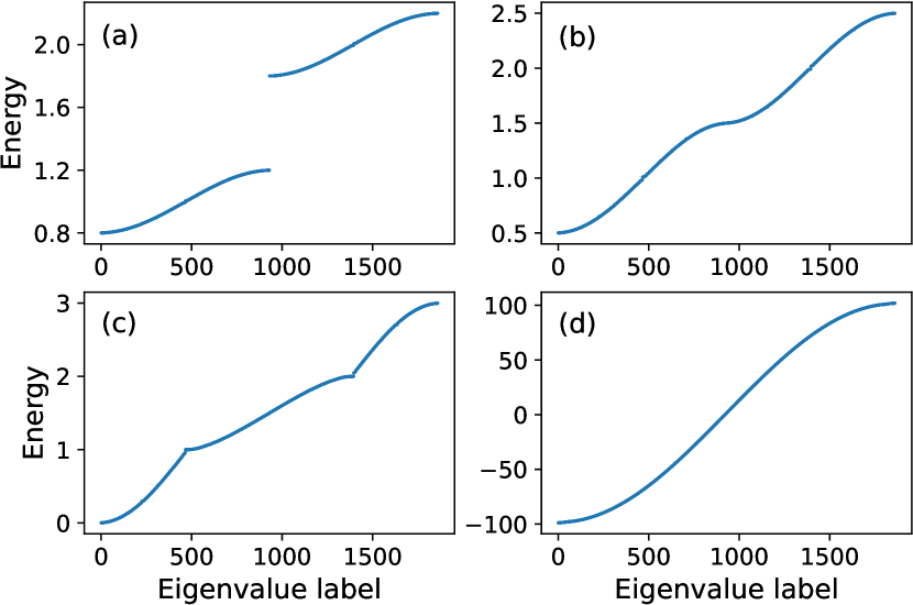
Figure 1: Spectrum of the energy eigenvalues for a SC. The onsite values used are $\epsilon_{A}=1,\epsilon_{B}=2$ and the off-diagonal coupling is varied according to $0.1,0.25,0.5,50.0$ from (a) to (d), respectively. Open boundary conditions and the length of the chain is $1861$.

The above discussion relates exclusively to the envelope or mean behavior of the spectrum. Let us now address the fluctuations of the energy levels which are well-characterized by the spacing of the energy levels. Fig.2 shows the spacing of the energy levels in a window of the spectrum between the energy levels $1570$ to $1730$. Notably we observe that the energy spacing covers several orders of magnitude. Interdispersed into seemingly irregular oscillations there is two types of prominent features. First we encounter minigaps in the spectrum corresponding to well-isolated distinguished peaks in Fig.2. Second, before and after those peaks we observe sequences of very small energy spacings lying on arcs. Examples for both features are indicated by arrows in Fig.2. Their origin will become clear in the context of the local resonator model to be developed in the next section.

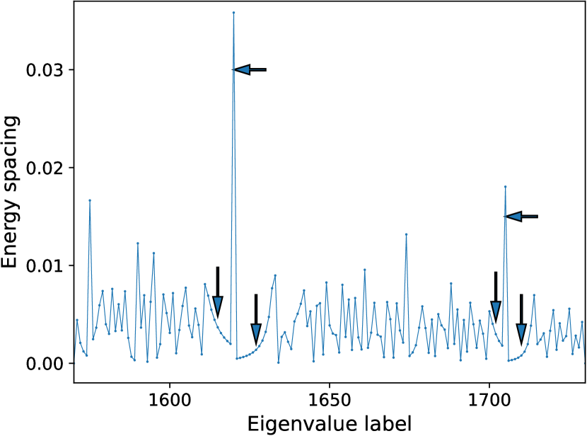
Figure 2: A finite spacing sequence (levels 1570 to 1730) of the energy eigenvalue spectrum for a SC. Arrows indicate two of the positions of the minigaps and four of the small spacing sequences located on corresponding arcs. The onsite values are $\epsilon_{A}=1,\epsilon_{B}=2$ and the off-diagonal coupling is $1.0$. Open boundary conditions and the length of the chain is $1861$.

In Fig.3 the energy spacing is shown for the complete eigenvalue spectrum for four different values of the coupling i.e. for $t=0.2,0.5,5.0,50.0$ in subfigures (a-d), respectively. For $t=0.2$ the eigenvalue spectrum is still gapped which reflects itself in a dominant peak of the spacing distribution at the position $930$, whose value is out of the scale provided in Fig.3(a). Left and right to this central peak there are two broad subdistributions with strongly fluctuating values for the spacings. On top of these subdistributions there is a central dominant peak as well as a number of additional prominent peaks which correspond to the above-mentioned minigaps in the spectrum. Those two branches of the spacing distributions are single humped and show monotonically decreasing spacings towards their edges.

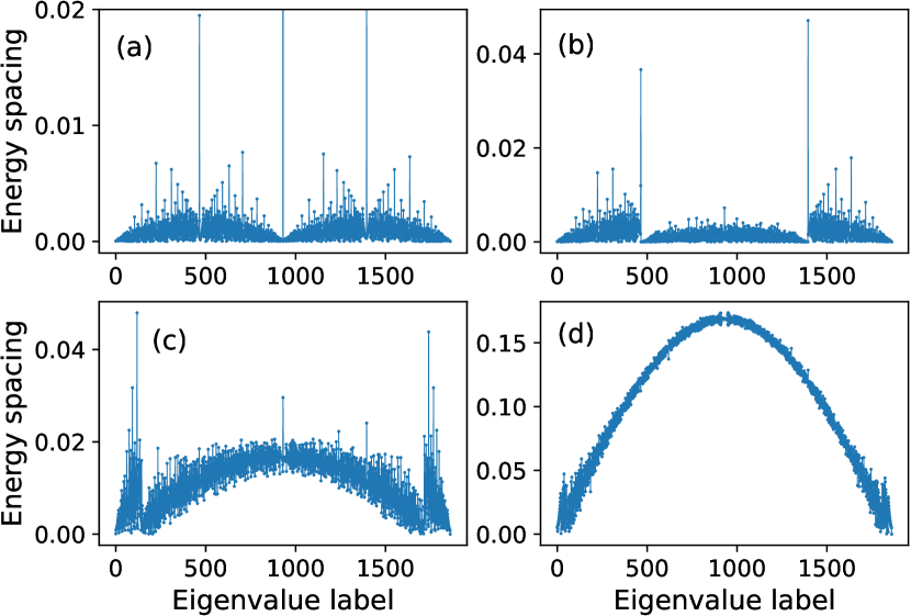
Figure 3: Spacing of the energy eigenvalue spectrum for a SC. The onsite values are $\epsilon_{A}=1,\epsilon_{B}=2$ and the off-diagonal coupling is varied according to $0.2,0.5,5.0,50.0$ from (a) to (d), respectively. Open boundary conditions and the length of the chain is $1861$.

Fig.3(b) corresponds to the case $t=0.5$ for which the eigenvalue spectrum possesses three branches (see Fig. 1(c)). Here the energy spacing distribution possesses also three distinct regions with abrupt transitions between them: the position of the transition points correspond to the positions of the cusps of the energy spectrum. At these positions of the cusps dominant peaks of the energy spacing occur followed by a collapse of the spacing behavior with further increasing degree of excitation in the spectrum. Overall the three branches encountered consist of two narrow semi-humps connected to the edges of the distribution and a complete broad hump in the center of the spacing distribution. With increasing coupling strength $t$ the central single-humped branch of the spacing distribution expands and finally represents the complete distributions. On this pathway the central branch bends upwards as is clearly visible in Fig.4(c,d) for $t=1.0,50.0$ implying that the spectrum of the spacing values possesses an increasing lower bound with increasing coupling strength. Finally, for $t=50.0$ in Fig.4(d) the spacing distribution is already rather similar to the one expected from the off-diagonal only case: it possesses a narrow width and only small fluctuations around the spacing values belonging to the spectrum $E_{m}=2t\cos(\frac{m\pi}{N+1})$ with $1\leq m\leq N$.

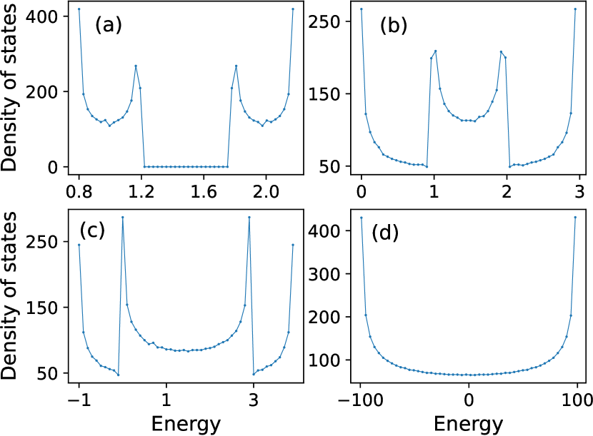
Figure 4: Density of states for a SC. The onsite values are $\epsilon_{A}=1,\epsilon_{B}=2$ and the off-diagonal coupling is varied according to $0.1,0.5,1.0,50.0$ from (a) to (d), respectively. Open boundary conditions and the length of the chain is $5101$.

Let us conclude this section by analyzing the energetical density of states (DOS) belonging to the SC for varying coupling strength $t$. For a periodic crystal of monomers the DOS can be obtained analytically to ${\cal{N}}(E)\propto\frac{1}{\sqrt{1-(\frac{E}{2t})^{2}}}$ possessing two singularities at the band edges and in between a smooth decrease followed by a corresponding increase. Fig.4(a) shows the case $t=0.1$ for which a sizeable gap between a low and high energy branch of the eigenvalue spectrum exists (see discussion of Fig.1). Correspondingly we observe four pronounced peaks for ${\cal{N}}(E)$ at the edge points of those two branches. In between the first two and the second two peaks a smooth decrease followed by a corresponding increase is encountered. The gap in the corresponding spectrum shows here up, of course, as a region of zero valued ${\cal{N}}(E)$. Fig.4(b) presents the DOS for $t=0.5$. Here the eigenvalue spectrum consists of three branches (see Fig.1(c)) and we observe two edge localized peaks and two peaks localized around the center of the DOS. The latter correspond to the positions of the cusps in the eigenvalue spectrum. Note that abrupt transitions occuring for the left and right side of the second and third peak of the DOS, respectively. For $t=1.0$ (Fig.4(c)) the central branch of the DOS has widened i.e. the corresponding central peaks have been moving towards the edges of the DOS thereby maintaining their narrow character. Finally, for $t=50.0$ only two peaks remain and are edge localized, as to be expected from the single branch case of an (approximately) off-diagonal only TB Hamiltonian.

IV Local resonator model

In order to develop a profound understanding of the above-discussed features of the eigenvalue spectrum, we develop a so-called local resonator model (LRM) for our SC. This model is inspired by the local symmetry theory of resonator structures developed in ref.Roentgen19 . In the latter work a quantitative analysis of the localization behavior of the eigenstates for strong and intermediate contrast has been provided for aperiodic binary chains based on substitution rules thereby focusing on the quasiperiodic case.

Our SC $1A,2B,2A,4B,4A,6B,6A,....2nB,2nA$ consists of a sequence of purely $A$ and $B$ subchains of increasing length with increasing size of the SC. We will call these subchains local resonators. Starting out with small values for the off-diagonal coupling $t$ we model the SC as a superposition of the spectra of these local $A$ and $B$ resonators. This is motivated by the fact that for zero coupling the resonators exhibit a degenerate spectrum which is splitted for small but finite coupling whereas the coupling between two different resonators is suppressed due to the substantial difference of their on-site energies $\epsilon_{A}=1.0$ and $\epsilon_{B}=2.0$. Employing open boundary conditions we therefore have the sequence of spectra for the local resonators as follows

$$E^{1}_{A}=E_{A}$$ (2)

$$E^{2}_{m}(A)=E_{A}+2t\cos\left(\frac{m\pi}{3}\right)\hskip 14.22636ptm=1,2$$

$$E^{2}_{m}(B)=E_{B}+2t\cos\left(\frac{m\pi}{3}\right)\hskip 14.22636ptm=1,2$$

$$E^{4}_{m}(A)=E_{A}+2t\cos\left(\frac{m\pi}{5}\right)\hskip 14.22636ptm=1,...,4$$

$$E^{4}_{m}(B)=E_{B}+2t\cos\left(\frac{m\pi}{5}\right)\hskip 14.22636ptm=1,...,4$$

$$...................................$$

$$E^{n}_{m}(A)=E_{A}+2t\cos\left(\frac{m\pi}{(n+1)}\right)\hskip 14.22636ptm=1,...,n$$

$$E^{n}_{m}(B)=E_{B}+2t\cos\left(\frac{m\pi}{(n+1)}\right)\hskip 14.22636ptm=1,...,n$$

The corresponding eigenstates are therefore localized resonator eigenstates. Note that their superposition is in general not an (even approximate) eigenstate of the SC, since the resonators possess different lengths. The total spectrum of the SC within this local resonator picture is given by

$$\Bigl{\{}E_{A},\Bigl{\{}E_{A}+2t\cos\left(\frac{m\pi}{(n+1)}\right)|n=2k,k\in[1,l],$$ (3)

$$m\in[1,n]\Bigr{\}}\Bigr{\}},\Bigl{\{}E_{B}+2t\cos\left(\frac{m\pi}{(n+1)}\right)|n=2k,$$

$$k\in[1,l],m\in[1,n]\Bigr{\}}\Bigr{\}}$$

where the length of the SC, i.e. the number of sites, is given by $N=1+2l(l+1)$ and the number of resonators in the SC is $2l+1$. The largest resonator consists of $2l$ sites. The envelope or mean behavior of the spectrum provided by our LRM agrees with many of the envelope features of the exact SC spectrum. E.g. it can describe the weak coupling broadening of the two bands, the subsequent closing of the energy gap as well as the emergence and widening of the third branch with increasing coupling. Even in the $t\rightarrow\infty$ limit which corresponds to a single branch case the spectral envelope behavior can qualitatively be reproduced. From the LRM we can draw some general conclusions. The size of the energy gap for not too strong coupling $t$ amounts to approximately $1-4t$ which means that the closing of the gap occurs for $t\approx 0.25$. The width of the central third branch for $t>0.25$ amounts to $4t-1$. Fig.5(a) shows a comparison of the LRM and the exact TB spectrum for a SC of length $221$ and for $t=1.0$: while the overall qualitative behavior is very similar one realizes significant deviations on smaller energy scales.

For this reason let us now analyze the energy eigenvalue spacing distribution of the LRM which provides us with the fluctuations of the energy levels. Fig.5(b) shows the spacing distribution for both the LRM and the exact TB spectrum for $t=0.1$. While the overall rough behavior is certainly similar, a closer look reveals remarkable deviations. The fluctuations are much stronger for the LRM compared to the TB results even for these small values of the coupling. A substantial number of the peak spacings agree within the two approaches and in particular the ’arc-like’ accumulation of small spacings around the main peaks is reproduced well. However, an eye-catching difference is the fact that the LRM shows zero spacings, corresponding to degeneracies in the LRM, whereas this is not the case for the TB spectrum. Considering the spectrum of the LRM in eq.(3) these degeneracies can be shown to occur for the set of 2-tuples satisfying for a given $m$ and $k$ and for varying $\alpha$

$$\begin{pmatrix}\alpha m\\ \alpha(2k+1)\\ \end{pmatrix}\hskip 14.22636pt\alpha\hskip 5.69046pt\hskip 5.69046pt\text{odd},\alpha\in\mathbb{N},m\leq 2k,k\leq l$$ (4)

Note that the eigenstates belonging to these degenerate eigenvalues belong in general to different local resonators. The lifting of these degeneracies in the TB spectrum is, of course, due to the interresonator coupling which is neglected within the LRM. An important remark is in order concerning the regime of stronger couplings $t>1$. In section III it has been shown that the center branch of the eigenvalue spacings exhibits an increasing upward bending with increasing coupling $t$ (see Fig.3(c,d)), meaning that the energy spacings systematically ’avoid small values’. This behavior cannot be described by the LRM, which shows its inadequacy in the strong coupling regime.

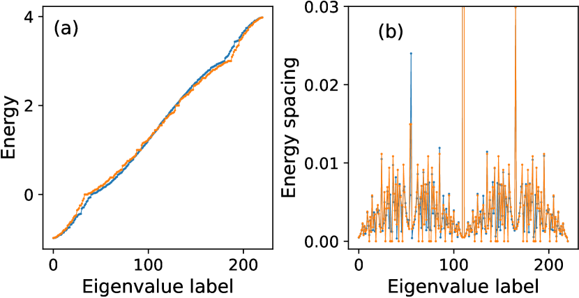
Figure 5: (a) Comparison of the eigenvalue spectrum and (b) of the energy spacing of the TB chain (blue) and its corresponding local resonator model (orange). The onsite values are $\epsilon_{A}=1,\epsilon_{B}=2$ and the off-diagonal coupling is $1.0$. Open boundary conditions and the length of the chain is $221$.

V Localization versus delocalization of eigenstates

Let us now focus on the analysis of the eigenstate properties of the SC for varying coupling strength $t$ with a particular emphasis on their localization properties. As described above in the framework of the LRM we expect for weak coupling strengths that the local resonator picture represents a good approximation and therefore the eigenstates should be localized within these resonators whose lengths increase monotonically along the SC. Fig.6(a) shows the eigenstate map, i.e. a greyscale image of the magnitudes of the components of the eigenstates with varying degree of excitation for the complete spectrum of a SC of length $221$ for $t=0.1$.

The ground state of the SC is localized on the largest $A$ local resonator of length $20$ appearing at the right end of the SC. The first excited state of the SC is localized on the second largest $A$ local resonator to the left of the ground state. This sequence continues (see Fig.6(a)) such that with increasing degree of excitation the corresponding eigenstates localize on local $A$ resonators with decreasing size, thereby moving from the right end towards the left end of the SC. This series of localized states are then intermingled with excited states of the local resonators which adds to the localization patterns observed in Fig.6(a). On the o.h.s. the spectrum can alternatively be described as follows. It consists of vertical series of localized resonator eigenstates whose energy spacings decrease with increasing size of the corresponding resonator. Series of localized resonator eigenstates of $A$ character belong to the low energy part of the spectrum whereas those of $B$ character belong to the high energy part. According to their occurence in the SC they are spatially shifted w.r.t. each other.

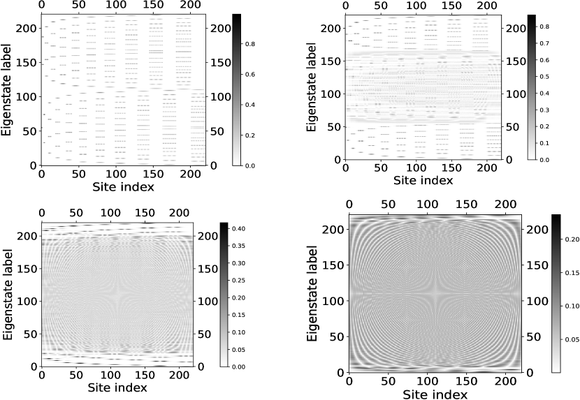
Figure 6: Eigenstate maps showing the absolute values of the eigenvector components of the scaled TB chain. The onsite values are $\epsilon_{A}=1,\epsilon_{B}=2$. The off-diagonal coupling is $0.1$ (upper left), $0.5$ (upper right), $5.0$ (lower left) and $50.0$ (lower right). Open boundary conditions and the length of the chain is $221$.

Inspecting the case $t=0.5$ in Fig.6(b) a branch of delocalized states can be observed for intermediate energies. This branch intensifies and broadens in energy with increasing coupling strength $t$. Indeed, for Figs.6(c,d) corresponding to $t=5.0,50.0$ the majority of eigenstates are delocalized over the complete SC. In conclusion, we obtain a distinct transition from series of localized resonator states for weak couplings to delocalized SC states for strong couplings which is controlled by the interresonator coupling of $A$ (low energy) and $B$ (high energy) character.

To quantify the above observations let us determine the inverse participation ratio (IPR) for the eigenstates on an SC with $N$ sites, which is defined as $r=\sum_{i=1}^{N}|\psi_{i}|^{4}\in[N^{-1},1]$ for a normalized eigenvector $\sum_{i=1}^{N}|\psi|^{2}=1$. The maximal value for the IPR is one for an eigenvector localized on a single site of the chain and the minimal value $\frac{1}{N}$ is encountered for a state which is uniformly extended over the chain. The IPR neither depends on the position at which a state is localized nor is it very sensitive to the details of its distribution.

Fig.7(a-d) shows the IPR for all eigenstates of the SC with length $221$ for four different values of the coupling strength $t=0.1,0.5,1.0,5.0$. For $t=0.1$ in Fig.7(a) the IPR has a lower bound of approximately $7\cdot 10^{-2}$ compared to the principally possible minimum of approximately $4.5\cdot 10^{-3}$. Most values are in the interval $[0.07,0.5]$ which indicates that the eigenstates are very localized. The sequence of local resonator localized states with increasing energy which have been analyzed in the context of the discussion of Fig.6 for $t=0.1$ can be seen here as a sequence of subsequent monotonically increasing IPR values. One can also observe sequences of almost constant values of the IPR which correspond to energetically non-neighboring eigenstates, i.e. among others involving the vertical series of localized states seen in Fig.6.

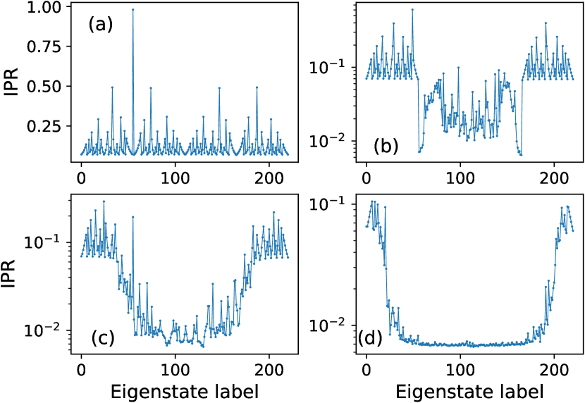
Figure 7: Inverse participation ratio (IPR) for all eigenstates of the SC. The onsite values are $\epsilon_{A}=1,\epsilon_{B}=2$. The off-diagonal coupling is $0.1,0.5,1.0,5.0$ for the subfigures (a)-(d), respectively. Open boundary conditions and the length of the chain is $221$.

For $t=0.5$ we observe a rather sharp decrease and a regime of low-values of the IPR in the central part of the spectrum. The latter branch of eigenstates corresponds to the delocalized states observed in the corresponding eigenstate maps of Fig.6. With further increasing values of $t$ (see Fig.7(c,d)) the IPR value of that average central plateau decreases monotonically and the fluctuations on top of it systematically decrease. Finally, at $t=50.0$, apart from a small window of states for very low and high energies, the IPR value is to a very good approximation constant and its value is close to the minimum possible value, i.e. it is approximately $6.5\cdot 10^{-3}$.

VI Transmission properties of the scaled TB chain

In this section we explore the energy-dependent transmission through our scaled tight-binding chain. To this end we attach two leads in the form of semi-infinite discrete chains to the left and right of our SC. Determining the transmission follows then the standard formalism of wave function matching Zwierzycki08 which folds the infinite leads into the SC and extends it by a single site to the left and to the right. In the language of Greens functions this corresponds to the inclusion of the corresponding self-energy into the Hamiltonian matrix problem: we map the closed system eigenvalue problem to a linear system of equations with an inhomogeneity Zwierzycki08 ; Datta95 ; Ferry97 . Note that the transmission is obtained as the absolute value squared of the $n+1$-st element of the vector obtained from the resulting linear equations.

As a result of the above procedure we have now the parameters $\epsilon_{L},t_{L},\epsilon_{R},t_{R},t_{LD},t_{DR}$ and $t,\epsilon_{A},\epsilon_{B}$. Here, $L,R$ stand for the corresponding quantities in the left and right lead: $\epsilon$ being the on-site energies and $t$ refering to the off-diagonal couplings, respectively. $t_{LD}$ is the coupling of the left lead to the scattering chain and $t_{DR}$ is the coupling of the scattering chain to the right lead, respectively. As done before we will use $\epsilon_{A}=1.0,\epsilon_{B}=2.0$.

The leads possess due to their semi-infinite structure a continuum of $k$-values. We focus on the case $t_{L/R}=1.0,\epsilon_{L/R}=1.0,t_{LD}=1.0,t_{DR}=1.0$. As a consequence the energy accessible in the left and right leads correspond to $E=\epsilon_{L/R}+2t_{L/R}\text{cos}(k_{L/R})$. Therefore we have $k\in[0,2\pi]$ and the lead energy window is $E\in[-1.0,3.0]$. We will then vary the coupling $t$ of the SC in the range $[0.1,50.0]$ and analyze the resulting transmission $T(E)$. For large values of $t$ the lead energy width will be small compared to the energetical width of the SC, whereas for small values of $t$ the opposite holds true.

In Fig.8(a-d) we show transmission spectra for the values $t=50.0,10.0,3.0,1.0$. For $t=50.0$ in Fig.8(a) the energy interval of the SC is approximately $[-99.0,102.0]$ and, as mentioned above, the lead energy interval is $[-1.0,3.0]$. Within this energy window the eigenstates of the isolated SC are all completely delocalized, see Fig.6. In this case the transmission spectrum shows three sharp peaks which are located approximately at the energies $E=0.0,1.5,3.0$. In between those peaks the transmission reaches approximately zero, i.e. the three peaks are well-isolated. This can be explained by projecting the energy window of the lead onto the stationary energy eigenvalue spectrum of the SC without leads only for the above parameters: Only three eigenstates located at the energies of the transmission peaks are encountered.

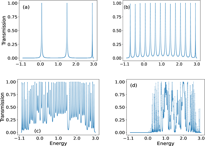
Figure 8: Transmission as a function of energy for the parameters $t_{L(R)}=\epsilon_{L(R)}=t_{LD}=t_{DR}=1.0$ and for $\epsilon_{A}=1.0,\epsilon_{B}=2.0$ for the scaled TB chain. The off-diagonal coupling is $50.0,10.0,3.0,1.0$ for the subfigures (a)-(d), respectively. Open boundary conditions and the length of the chain is $221$.

If we now decrease the value of the coupling to $t=10.0$ (see Fig.8(b)), we have an energy window of approximately $[-19.0,22.0]$ for the SC, and we observe $14$ distinct peaks. In between this dense sequence of well-isolated peaks the transmission does not completely decrease to the value zero due to the finite overlap of the resonances. As a result the transmission peaks ’live’ on a background of low transmission. Again, this series of transmission peaks can be understood by projecting the energy window of the lead $E\in[-1.0,3.0]$ onto the energy eigenvalue spectrum of the SC for $t=10.0$. The corresponding eigenstates of the SC without leads are assignable to the transmission one peaks and are of completely delocalized character. The above trend continues with e.g. for $t=5.0$ 28 peaks (not shown) being present in the transmission spectrum. The background transmission increases consequently. Also for $t=3.0$ (see Fig.8(c)) we address with the lead energy window only delocalized states. The transmission spectrum shows still a series of distinct peaks, but with a larger more irregular appearing background formed by the overlaping resonances.

For $t=1.0$ (see Fig.8(d)) the transmission profile has changed qualitatively. Now, the lead energy window $[-1.0,3.0]$ covers a large part of the energy eigenvalue spectrum and the corresponding states are for low energy purely localized whereas for $E\gtrsim 0.2$ they become delocalized and contribute to the highly irregular transmission profile. The delocalized part of the eigenstates ends at $E\approx 3.0$ which is also the end of the transmission energy window. While the transmission spectrum is irregular, there is, in many cases, a clear assignment to the behavior of the inverse participation ratio: low values of the IPR correspond to delocalization which leads to high transmission values. For $t=0.5$ (not shown here) the transmission profile is even more fragmented into irregular series of narrow peaks and finally, for $t=0.3$, the transmission is essentially zero in the complete spectral window.

VII Summary and conclusions

The concept of local symmetry dynamics provides a systematic pathway of generating lattices covered with overlapping local symmetries. While this pathway has very recently been pursued to show that the class of so-called $n:m$ rules provide us with emergent periodic behavior Schmelcher23 , we show here that the local symmetry dynamics according to the rule $n,(n+1),(n+2),(n+3),...$ leads (for $n=2$) to a scaling behavior. The resulting chain consists therefore of the concatenation of alternating subchains of increasing lengths.

Mapping the scaled chain onto a tight binding Hamiltonian the focus of the present work has been on the analysis of the spectral and transmission properties of this Hamiltonian. The energy eigenvalue spectrum shows with increasing strength of the off-diagonal coupling a transition from two to three and finally to a single branch. A closer look at the spectrum reveals minigaps accompanied by a characteristic accumulation of eigenvalues in their neighborhood. The eigenvalue spacings exhibit a crossover from the case of a two to a three and finally a single humped distribution. The cusps connecting the different branches go along with sharp peaks in the corresponding density of states. Many of the features occuring for the eigenvalue spectrum could be explained and understood via a local resonator model which applies for weak to intermediate values of the coupling and which treats the subchains possessing the same on-site energies as independent resonators. The spectrum and eigenstates of the complete chain are then composed of the independent resonator spectra and eigenstates. Indeed, an eigenstate analysis via so-called eigenstate maps demonstrates the localization of the eigenstates in terms of resonator eigenmodes for weak couplings. The transition to delocalization with increasing coupling strengths occurs in an expanding manner starting from the center of the spectrum and has been analyzed via the corresponding behavior of the inverse participation ratio. Finally, we have investigated the transmission properties of the scaled chain and found, with decreasing coupling, a transition from the case of a few regularly arranged isolated transmission one peaks to the case of many such peaks on an enhanced background. Finally, for sufficiently small coupling strengths, the transmission profile becomes highly irregular and probes the complete delocalized eigenstate portion of the scaled chain.

The presently investigated case of a scaled chain is certainly only a specific case out of many possible local symmetry dynamics generated chains which are asymptotically non-periodic. Indeed, one can think of many different ways of modifying the applied rule such that a rich interplay of scaled subchains with intermediate ones appear. The common feature of all of those chains is the presence of the extensive local reflection symmetries of overlapping character. It is left to future investigations to possibly arrive at a classification of those local symmetry dynamics generated lattices and the physical properties of their resulting tight binding realizations.

Finally let us briefly address the possibility of an experimental realization of the scaled tight-binding chain. A promising optics-based platform are evanescently coupled waveguides (see ref.Szameit10 and in particular the references therein). Due to the extended control of the underlying optical materials the propagation of light and the coupling among the waveguides can be varied in a wide range and the dynamical evolution has many commons with the corresponding time evolution for a single particle quantum system. The coupling among the waveguides can be encoded into the bulk material using femtosecond laser pulses. A limiting factor for the current application to the scaled chain is certainly the number of waveguides accessible which would correspondingy limit the largest possible resonator in the chain.

VIII Acknowledgments

This work has been supported by the Cluster of Excellence “Advanced Imaging of Matter” of the Deutsche Forschungsgemeinschaft (DFG)-EXC 2056, Project ID No. 390715994.

References

- (1) J.P. Sethna, 1991 Lectures in Complex Systems, Eds. L. Nagel and D. Stein, Santa Fe Institute Studies in the Sciences of Complexity, Proc. Vol. XV, Addison-Wesley 1992.
- (2) The rise of quantum materials, Editorial, Nature Physics 12, 105 (2016).
- (3) D.J. Gross, The role of symmetry in fundamental physics, Proc.Nat.Acad.Sc. 93, 14256 (1996).
- (4) N.W. Ashcroft and N.D. Mermin, Solid State Physics, Holt-Saunders, 1976.
- (5) J. Singleton, Band Theory and Electronic Properties of Solids, Oxford Master Series in Condensed Matter Physics, Oxford University Press 2001.
- (6) E. Maciá Barber, Aperiodic Structures in Condensed Matter, Fundamentals and Applications, Series in Condensed Matter Physics, CRC Press 2009.
- (7) E. Maciá-Barber, Quasicrystals, Fundamentals and Applications, CRC Press 2021.
- (8) D. Shechtman, I. Blech, D. Gratias, and J. W. Cahn, Metallic phase with long-range orientational order and no translational symmetry, Phys.Rev.Lett. 53, 1951 (1984).
- (9) J.B. Suck, M. Schreiber, P. Häussler, Quasicrystals: An Introduction to Structure, Physical Properties and Applications, Springer Science & Business Media 2002.
- (10) C. Morfonios, P. Schmelcher, P.A. Kalozoumis and F.K. Diakonos, Local symmetry dynamics in one-dimensional aperiodic lattices: a numerical study, Nonl.Dyn. 78, 71 (2014).
- (11) P.A. Kalozoumis, C. Morfonios, F.K. Diakonos and P. Schmelcher, Invariant of broken discrete symmetries, Phys.Rev.Lett. 113, 050403 (2014).
- (12) P.A. Kalozoumis, C. Morfonios, F.K. Diakonos and P. Schmelcher, Local symmetries in one-dimensional quantum scattering, Phys.Rev.A 87, 032113 (2013); P.A. Kalozoumis, C. Morfonios, N. Palaiodimopoulos, F.K. Diakonos and P. Schmelcher, Local symmetries and perfect transmission in aperiodic photonic multilayers, Phys.Rev.A 88, 033857 (2013).
- (13) C. Morfonios, P.A. Kalozoumis, F.K. Diakonos and P. Schmelcher, Nonlocal discrete continuity and invariant currents in locally symmetric effective Schrödinger arrays, Ann.Phys. 385, 623 (2017).
- (14) P. Schmelcher, S. Krönke and F.K. Diakonos, Dynamics of local symmetry correlators for interacting many-particle systems, J.Chem.Phys. 146, 044116 (2017).
- (15) V.E. Zambetakis, M.K. Diakonou, P.A. Kalozoumis, F.K. Diakonos, C.V. Morfonios, P. Schmelcher, Invariant current approach to wave propagation in locally symmetric structures, J.Phys.A 49, 195304 (2016).
- (16) P.A. Kalozoumis, O. Richoux, F. K. Diakonos, G. Theocharis, and P. Schmelcher, Invariant currents in lossy acoustic waveguides with complete local symmetry, Phys.Rev.B 92, 014303 (2015).
- (17) N. Schmitt, S. Weimann, C.V. Morfonios, M. Röntgen, M. Heinrich, P. Schmelcher and A. Szameit, Observation of Local Symmetry in Photonic Systems, Las.Phot.Rev. 14, 1900222 (2020).
- (18) C.V. Morfonios, M. Röntgen, F.K. Diakonos and P. Schmelcher, Transfer efficiency enhancement and eigenstate properties in locally symmetric disordered finite chains, Ann.Phys. 418, 168163 (2020).
- (19) M. Röntgen, C.V. Morfonios, R. Wang, L. Dal Negro and P. Schmelcher, Local symmetry theory of resonator structures for the real-space control of edge states in binary aperiodic chains, Phys.Rev. B 99, 214201 (2019).
- (20) P. Schmelcher, Evolution of discrete symmetries, arXiv:2303.14150v1.
- (21) C.M. Goringe, D.R. Bowler and E. Hernández, Tight-binding modelling of materials, Rep.Progr.Phys. 60, 1447 (1997).
- (22) S. Kouachi, Eigenvalues and eigenvectors of tridiagonal matrices, El.J.Lin.Alg. 15, 115 (2006).
- (23) D. Kulkarni, D. Schmidt and S.-K. Tsui, Eigenvalues of tridiagonal pseudo-Toeplitz matrices, Lin.Alg.Appl. 297, 63 (1999).
- (24) A.R. Willms, Analytic results for the eigenvalues of certain tridiagonal matrices, Siam J.Matrix Anal.Appl. 30, 639 (2008).
- (25) M. Zwierzycki et al, Phys.Stat.Sol. 245, 623 (2008).
- (26) S. Datta, Electronic Transport in Mesoscopic Systems, Cambridge University Press 1995.
- (27) D.K. Ferry and S.M. Goodnick, Transport in Nanostructures, Cambridge University Press 1997.
- (28) A. Szameit and S. Nolte, Discrete optics in femtosecond-laser-written photonic structures, J. Phys. B 43, 163001 (2019).