SparqLog: A System for Efficient Evaluation of SPARQL 1.1 Queries via Datalog [Experiment, Analysis & Benchmark]

Abstract.

Over the past decade, Knowledge Graphs have received enormous interest both from industry and from academia. Research in this area has been driven, above all, by the Database (DB) community and the Semantic Web (SW) community. However, there still remains a certain divide between approaches coming from these two communities. For instance, while languages such as SQL or Datalog are widely used in the DB area, a different set of languages such as SPARQL and OWL is used in the SW area. Interoperability between such technologies is still a challenge. The goal of this work is to present a uniform and consistent framework meeting important requirements from both, the SW and DB field.

PVLDB Reference Format:
PVLDB, 14(1): XXX-XXX, 2022.
doi:XX.XX/XXX.XX

PVLDB Artifact Availability:
The source code, data, and/or other artifacts have been made available at URL_TO_YOUR_ARTIFACTS.

1. Introduction

Since Google launched its Knowledge Graph (KG) roughly a decade ago, we have seen intensive work on this topic both in industry and in academia. However, there are two research communities working mostly isolated from each other on the development of KG management systems, namely the Database and the Semantic Web community. Both of them come with their specific key requirements and they have introduced their own approaches.

Of major importance to the Semantic Web (SW) community is the compliance with the relevant W3C standards:

[RQ1] SPARQL Feature Coverage. The query language SPARQL is one of the major Semantic Web standards. Therefore, we require the support of the most commonly used SPARQL features.
[RQ2] Bag Semantics. SPARQL employs per default bag semantics (also referred to as multiset semantics) unless specified otherwise in a query. We therefore require the support of this.

[RQ3] Ontological Reasoning. OWL 2 QL to support ontological reasoning is a major Semantic Web standard. Technically, for rule-based languages, this means that existential quantification (i.e., “object invention”) in the rule heads is required.

The Database (DB) community puts particular emphasis on the expressive power and efficient evaluation of query languages. This leads us to the following additional requirement:

[RQ4] Full Recursion. Full recursion is vital to provide the expressive power needed to support complex querying in business applications and sciences (see e.g., (Przymus et al., 2010)) and it is the main feature of the relational query language Datalog (Vianu, 2021). Starting with SQL-99, recursion has also been integrated into the SQL standard and most relational database management systems have meanwhile incorporated recursion capabilities to increase their expressive power.

Finally, for an approach to be accepted and used in practice, we formulate the following requirement for both communities:

[RQ5] Implemented System. Both communities require an implemented system. This makes it possible to verify if the theoretic results are applicable in practice and to evaluate the usefulness of the approach under real-world settings.

The above listed requirements explain why there exists a certain gap between the SW and DB communities. There have been several attempts to close this gap. However, as will be detailed in Section 2, no approach has managed to fulfil the requirements of both sides so far. Indeed, while existing solutions individually satisfy some of the requirements listed above, all of them fail to satisfy central other requirements. The goal of this work is to develop one uniform and consistent framework that satisfies the requirements of both communities. More specifically, our contributions are as follows:

Theoretical Translation. We provide a uniform and complete framework to integrate SPARQL support into a KG language that meets all of the above listed requirements RQ1–RQ5. We have thus extended, simplified and – in some cases – corrected previous approaches of translating SPARQL queries (under both set and bag semantics) to various Datalog dialects (Polleres, 2007; Polleres and Wallner, 2013; Angles and Gutiérrez, 2016a). For instance, to the best of our knowledge, all previous translations have missed or did not consider correctly certain aspects of the SPARQL standard of the zero-or-one and zero-or-more property paths.

Translation Engine. We have developed the translation engine SparqLog on top of the Vadalog system that covers most of the considered SPARQL 1.1 functionality. We thus had to fill several gaps between the abstract theory and the practical development of the translation engine. For instance, to support bag semantics, we have designed specific Skolem functions to generate a universal duplicate preservation process. On the other hand, the use of the Vadalog system as the basis of our engine made significant simplifications possible (such as letting Vadalog take care of complex filter constraints) and we also get ontological reasoning “for free”. SparqLog therefore supports both query answering and ontological reasoning in a single uniform and consistent system.

Experimental Evaluation. We carry out an extensive empirical evaluation on multiple benchmarks with two main goals in mind: to verify the compliance of SparqLog with the SPARQL standard as well as to compare the performance of our system with comparable ones. It turns out that, while SparqLog covers a great part of the selected SPARQL 1.1 functionality in the correct way, some other systems (specifically Virtuoso) employ a non-standard behaviour on queries containing property paths. As far as query-execution times are concerned, the performance of SparqLog is, in general, comparable to other systems such as the SPARQL system Fuseki or the querying and reasoning system Stardog and it significantly outperforms these systems on complex queries containing recursive property paths and/or involving ontologies.

Structure of the paper. After a review of existing approaches in Section 2, and the preliminaries in Section 3, we present our main results: the general principles of our SparqLog system in Section 4, a more detailed look into the translation engine in Section 5, and an experimental evaluation in Section 6. We conclude with Section 7. Further details on our theoretical translation, implementation, and experimental results are provided in the appendix.

2. Related Approaches

We review several approaches – both from the Semantic Web and the Database community. This discussion of related approaches is divided into theoretical and practical aspects of our work.

2.1. Theoretical Approaches

Several theoretical research efforts have aimed at bridging the gap between the DB and SW communities.

Translations of SPARQL to Answer Set Programming. In a series of papers, Polleres et al. presented translations of SPARQL and SPARQL 1.1 to various extensions of Datalog. The first translation from SPARQL to Datalog (Polleres, 2007) converted SPARQL queries into Datalog programs by employing negation as failure. This translation was later extended by the addition of new features of SPARQL 1.1 and by considering its bag semantics in (Polleres and Wallner, 2013). Thereby, Polleres and Wallner created a nearly complete translation of SPARQL 1.1 queries to Datalog with disjunction (DLV) programs. However, the translation had two major drawbacks: On the one hand, the chosen target language DLV does not support ontological reasoning as it does not contain existential quantification, thereby missing a key requirement (RQ3) of the Semantic Web community. On the other hand, the requirement of an implemented system (RQ5) is only partially fulfilled, since the prototype implementation DLVhex-SPARQL Plugin (Polleres and Schindlauer, 2007) of the SPARQL to Datalog translation of (Polleres, 2007) has not been extended to cover also SPARQL 1.1 and bag semantics.
Alternative Translations of SPARQL to Datalog. An alternative approach of relating SPARQL to non-recursive Datalog with stratified negation (or, equivalently, to Relational Algebra) was presented by Angles and Gutierrez in (Angles and Gutiérrez, 2008). The peculiarities of negation in SPARQL were treated in a separate paper (Angles and Gutiérrez, 2016b). The authors later extended this line of research to an exploration of the bag semantics of SPARQL and a characterization of the structure of its algebra and logic in (Angles and Gutiérrez, 2016a). They translated a few SPARQL features into a Datalog dialect with bag semantics (multiset non-recursive Datalog with safe negation). This work considered only a small set of SPARQL functionality on a very abstract level and used again a target language that does not support ontological reasoning, failing to meet important requirements (RQ1, RQ3) of the SW community. Most importantly, no implementation exists of the translations provided by Angles and Gutierrez, thus failing to fulfil RQ5.
Supporting Ontological Reasoning via Existential Rules. In (Calì et al., 2009), Datalog^± was presented as a family of languages that are particularly well suited for capturing ontological reasoning. The “$+$” in Datalog^± refers to the crucial extension compared with Datalog by existential rules, that is, allowing existentially quantified variables in the rule heads. However, without restrictions, basic reasoning tasks such as answering Conjunctive Queries w.r.t. an ontology given by a set of existential rules become undecidable (Johnson and Klug, 1984). Hence, numerous restrictions have been proposed (Fagin et al., 2005; Calì et al., 2013, 2010, 2010; Baget et al., 2009; Baget et al., 2011) to ensure decidability of such tasks, which led to the “$-$“ in Datalog^±. Of all variants of Datalog^±, Warded Datalog^± (Arenas et al., 2018) ultimately turned out to constitute the best compromise between complexity and expressiveness and it has been implemented in an industrial-strength system – the Vadalog system (Bellomarini et al., 2018), thus fulfilling requirement RQ5. However, the requirement of supporting SPARQL (RQ1) with or without bag semantics (RQ2) have not been fulfilled up to now.
Warded Datalog^± with Bag Semantics. In (Bertossi et al., 2019), it was shown that Warded Datalog^± using set semantics can be used to represent Datalog using bag semantics by using existential quantification to introduce new tuple IDs. It was assumed that these results could be leveraged for future translations from SPARQL with bag semantics to Warded Datalog^± with set semantics. However, the theoretical translation of SPARQL to Vadalog (RQ1) using these results and also implementation (RQ5) by extending Vadalog were left open in (Bertossi et al., 2019) and considered of primary importance for future work.

2.2. Practical Approaches

Several systems have aimed at bridging the gap between DB and SW technologies. The World Wide Web Consortium (W3C) lists StrixDB, DLVhex SPARQL-engine and RDFox as systems that support SPARQL in combination with Datalog. Furthermore, we also have a look at ontological reasoning systems Vadalog, Graal and VLog, which either understand SPARQL to some extent or, at least in principle, could be extended in order to do so.
DLVhex-SPARQL Plugin. As mentioned above, the DLVhex-SPARQL Plugin (Polleres and Schindlauer, 2007) is a prototype implementation of the SPARQL to Datalog translation in (Polleres, 2007). According to the repository’s ReadMe file, it supports basic graph patterns, simple conjunctive FILTER expressions (such as ISBOUND, ISBLANK, and arithmetic comparisons), the UNION, OPTIONAL, and JOIN operation. Other operations, language tags, etc. are not supported and query results do not conform to the SPARQL protocol, according to the ReadMe file. Moreover, the underlying logic programming language DLV provides only domain specific existential quantification (described in (Eiter et al., 2013)), produced e.g. by hash-functions. Hence, it only provides very limited support of existential quantification, which does not suffice for ontological reasoning as required by the OWL 2 QL standard (RQ3). Also the support of bag semantics is missing (RQ2).
RDFox. RDFox is an RDF store developed and maintained at the University of Oxford (Nenov et al., 2015). It reasons over OWL 2 RL ontologies in Datalog and computes/stores materialisations of the inferred consequences for efficient query answering (Nenov et al., 2015). The answering process of SPARQL queries is not explained in great detail, except stating that queries are evaluated on top of these materialisations, by employing different scanning algorithms (Nenov et al., 2015). However, translating SPARQL to Datalog – one of the main goals of this paper – is not supported. Moreover, RDFox does currently not support property paths and some other SPARQL 1.1 features.

StrixDB. StrixDB is an RDF store developed as a simple tool for working with middle-sized RDF graphs, supporting SPARQL 1.0 and Datalog reasoning capabilities. To the best of our knowledge, there is no academic paper or technical report that explains the capabilities of the system in greater detail – leaving us with the web page as the only source of information on StrixDB. The StrixStore documentation page lists examples of how to integrate Datalog rules into SPARQL queries, to query graphs enhanced by Datalog ontologies. However, translating SPARQL to Datalog – one of the main goals of this paper – is not supported. Moreover, important SPARQL 1.1 features such as aggregation and property paths are not supported by StrixDB.
Graal. Graal was developed as a toolkit for querying ontologies with existential rules (Baget et al., 2015). The system does not focus on a specific storage system, however specializes in algorithms that can answer queries regardless of the underlying database type (Baget et al., 2015). It reaches this flexibility, by translating queries from their host system language into Datalog^±. However, it pays the trade-off of restricting itself to answering conjunctive queries only (Baget et al., 2015) and therefore supports merely a small subset of SPARQL features — e.g. not even being able to express basic features such as UNION or MINUS. Clearly, the goal of developing a uniform and consistent framework for both, the Semantic Web and Database communities, cannot be achieved without supporting at least the most vital features of SPARQL (RQ1).

VLog. VLog is a rule engine, developed at the TU Dresden (Carral et al., 2019). The system transfers incoming SPARQL queries to specified external SPARQL endpoints such as Wikidata and DBpedia and incorporates the received query results into their knowledge base (Carral et al., 2019). Therefore, the responsibility of query answering is handed over to RDF triple stores that provide a SPARQL query answering endpoint, thus failing to provide a uniform, integrated framework for combining query answering with ontological reasoning (RQ5).

The Vadalog system (Bellomarini et al., 2018) is a KG management system implementing the logic-based language Warded Datalog^±. It extends Datalog by including existential quantification necessary for ontological reasoning, while maintaining reasonable complexity. As an extension of Datalog, it supports full recursion. Although Warded Datalog^± has the capabilities to support SPARQL 1.1 under the OWL 2 QL entailment regime (Arenas et al., 2018) (considering set semantics though!), no complete theoretical nor any practical translation from SPARQL 1.1 to Warded Datalog^± exists. Therefore, the bag semantics (RQ2) and SPARQL feature coverage (RQ1) requirements are not met.

3. Preliminaries

3.1. RDF and SPARQL

RDF (Cyganiak et al., 2014) is a W3C standard that defines a graph data model for describing Web resources. The RDF data model assumes three data domains: IRIs that identify Web resources, literals that represent simple values, and blank nodes that identify anonymous resources. An RDF triple is a tuple $(s,p,o)$, where $s$ is the subject, $p$ is the predicate, $o$ is the object, all the components can be IRIs, the subject and the object can alternatively be a blank node, and the object can also be a literal. An RDF graph is a set of RDF triples. A named graph is an RDF graph identified by an IRI. An RDF dataset is a structure formed by a default graph and zero or more named graphs.

For example, consider that <http://example.org/graph.rdf> is an IRI that identifies an RDF graph with the following RDF triples:

<http://ex.org/glucas> <http://ex.org/name> "George"
<http://ex.org/glucas> <http://ex.org/lastname> "Lucas"
_:b1 <http://ex.org/name> "Steven"

This graph describes information about film directors. Each line is an RDF triple, <http://ex.org/glucas> is an IRI, "George" is a literal, and _:b1 is a blank node.

SPARQL (Prud’hommeaux and Seaborne, 2008; Harris and Seaborne, 2013) is the standard query language for RDF. The general structure of a SPARQL query is shown in Figure 1, where: the SELECT clause defines the output of the query, the FROM clause defines the input of the query (i.e. an RDF dataset), and the WHERE clause defines a graph pattern.

1SELECT ?N ?L2FROM <http://example.org/graph.rdf>3WHERE { ?X <http://ex.org/name> ?N4         . OPTIONAL { ?X <http://ex.org/lastname> ?L }}5ORDER BY ?N

Figure 1. Example of SPARQL query.

The evaluation of a query begins with the construction of the RDF dataset to be queried, whose graphs are defined by one or more dataset clauses. A dataset clause is either an expression $\operatorname{FROM}$ $u$ or $\operatorname{FROM~{}NAMED}$ $u$, where $u$ is an IRI that refers to an RDF graph. The former clause merges a graph into the default graph of the dataset, and the latter adds a named graph to the dataset.

The $\operatorname{WHERE}$ clause defines a graph pattern (GP). There are many types of GPs: triple patterns (RDF triples extended with variables), basic GPs (a set of GPs), optional GPs, alternative GPs (UNION), GPs on named graphs (GRAPH), negation of GPs (NOT EXISTS and MINUS), GPs with constraints (FILTER), existential GPs (EXISTS), and nesting of GPs (SubQueries). A property path is a special GP which allows to express different types of reachability queries.

The result of evaluating a graph pattern is a multiset of solution mappings. A solution mapping is a set of variable-value assignments. E.g., the evaluation of the query in Figure 1 over the above RDF graph returns two mappings $\{\mu_{1},\mu 2\}$ with $\mu_{1}$(?N) $=$ "George", $\mu_{1}$(?L) $=$ "Lucas" and $\mu_{1}$(?N) $=$ "Steven".

The graph pattern matching step returns a multiset whose solution mappings are treated as a sequence without specific order. Such a sequence can be arranged by using solution modifiers: $\operatorname{ORDER~{}BY}$ allows to sort the solutions; $\operatorname{DISTINCT}$ eliminates duplicate solutions; $\operatorname{OFFSET}$ allows to skip a given number of solutions; and $\operatorname{LIMIT}$ restricts the number of output solutions.

Given the multiset of solution mappings, the final output is defined by a query form: $\operatorname{SELECT}$ projects the variables of the solutions; $\operatorname{ASK}$ returns $\operatorname{\emph{true}}$ if the multiset of solutions is non-empty and $\operatorname{\emph{false}}$ otherwise; $\operatorname{CONSTRUCT}$ returns an RDF graph whose content is determined by a set of triple templates; and $\operatorname{DESCRIBE}$ returns an RDF graph that describes the resources found.

3.2. Warded Datalog^± and the Vadalog System

In (Calì et al., 2009), Datalog^± was presented as a family of languages that extend Datalog (whence the $+$) to increase its expressive power but also impose restrictions (whence the $-$) to ensure decidability of answering Conjunctive Queries (CQs). The extension most relevant for our purposes is allowing existential rules of the form

$\exists\bar{z}P(\bar{x}^{\prime},\bar{z})\ \leftarrow\ P_{1}(\bar{x}_{1}),\ldots,P_{n}(\bar{x}_{n})$,

with $\bar{x}^{\prime}\subseteq\bigcup_{i}\bar{x}_{i}$, and $\bar{z}\cap\bigcup_{i}\bar{x}_{i}=\emptyset$. Datalog^± is thus well suited to capture ontological reasoning. Ontology-mediated query answering is defined by considering a given database $D$ and program $\Pi$ as logical theories. The answers to a CQ $Q(\vec{z})$ with free variables $\vec{z}$ over database $D$ under the ontology expressed by Datalog^± program $\Pi$ are defined as $\{\vec{a}\mid\Pi\cup D\models Q(\vec{a})\}$, where $\vec{a}$ is a tuple of the same arity as $\vec{z}$ with values from the domain of $D$.

Several subclasses of Datalog^± have been presented (Fagin et al., 2005; Calì et al., 2013, 2010, 2010; Baget et al., 2009; Baget et al., 2011; Arenas et al., 2018) that ensure decidability of CQ answering (see (Calì et al., 2013) for an overview). One such subclass is Warded Datalog^± (Arenas et al., 2018), which makes CQ answering even tractable (data complexity). For a formal definition of Warded Datalog^±, see (Arenas et al., 2018). We give the intuition of Warded Datalog^± here. First, for all positions in rules of a program $\Pi$, distinguish if they are affected or not: a position is affected, if the chase may introduce a labelled null here, i.e., a position in a head atom either with an existential variable or with a variable that occurs only in affected positions in the body. Then, for variables occurring in a rule $\rho$ of $\Pi$, we identify the dangerous ones: a variable is dangerous in $\rho$, if it may propagate a null in the chase, i.e., it appears in the head and all its occurrences in the body of $\rho$ are at affected positions. A Datalog^± program $\Pi$ is warded if all rules $\rho\in\Pi$ satisfy: either $\rho$ contains no dangerous variable or all dangerous variables of $\rho$ occur in a single body atom $A$ (= the “ward”) such that the variables shared by $A$ and the remaining body occur in at least one non-affected position (i.e., they cannot propagate nulls).

Apart from the favourable computational properties, another important aspect of Warded Datalog^± is that a full-fledged engine (even with further extensions) exists: the Vadalog system (Bellomarini et al., 2018). It combines full support of Warded Datalog^± plus a number of extensions needed for practical use, including (decidable) arithmetics, aggregation, and other features. It has been deployed in numerous industrial scenarios, including the finance sector as well as the supply chain and logistics sector.

4. The SparqLog System

This section introduces SparqLog, a system that allows to evaluate SPARQL 1.1 queries on top of the Vadalog system. To the best of our knowledge, SparqLog is the first system that provides a complete translation engine from SPARQL 1.1 with bag semantics to Datalog. In order to obtain a functional and efficient system, we combined the knowledge provided by the theoretical work with database implementation techniques.

SparqLog implements three translation methods: (i) a data translation method $T_{D}$ which generates Datalog^± rules from an RDF Dataset; (ii) a query translation method $T_{Q}$ which generates Datalog^± rules from a SPARQL query; and (iii) a solution translation method $T_{S}$ which generates a SPARQL solution from a Datalog^± solution. Hence, given an RDF dataset $D$ and a SPARQL query $Q$, SparqLog generates a Datalog^± program $\Pi$ as the union of the rules returned by $T_{D}$ and $T_{Q}$, then evaluates the program $\Pi$, and uses $T_{S}$ to transform the resulting Datalog^± solution into a SPARQL solution.

4.1. Example of Graph Pattern Translation

In order to give a general idea of the translation, we will sketch the translation of the RDF graph and the SPARQL query presented in Section 3.1. To facilitate the notation, we will abbreviate the IRIs by using their prefix-based representation. For example, the IRI http://ex.org/name will be represented as ex:name, where ex is a prefix bound to the namespace http://ex.org/. Additionally, we will use graph.rdf instead of http://example.org/graph.rdf.

4.1.1. Data translation

Consider the RDF graph $G$ presented in Section 3.1. First, the data translation method $T_{D}$ generates a special fact for every RDF term (i.e., IRI, literal, and blank node) in $G$:

iri("ex:glucas"). iri("ex:name"). iri("ex:lastname").
literal("George"). literal("Lucas"). literal("Steven").
bnode("b1").

These facts are complemented by the following rules, which represent the domain of RDF terms:

term(X) :- iri(X).
term(X) :- literal(X).
term(X) :- bnode(X).

For each RDF triple (s,p,o) in graph $G$ with IRI g, $T_{D}$ generates a fact triple(s,p,o,g). Hence, in our example, $T_{D}$ produces:

triple("ex:glucas", "ex:name", "George", "graph.rdf").
triple("ex:glucas", "ex:lastname", "Lucas", "graph.rdf").
triple("b1", "ex:name", "Steven", "graph.rdf").

4.1.2. Query translation

Assume that $Q$ is the SPARQL query presented in Figure 1. The application of the query translation method $T_{Q}$ over $Q$ returns the Datalog^± rules shown in Figure 2. The general principles of the translation will be discussed in Section 5.1. In the interest of readability, we slightly simplify the presentation, e.g., by omitting language tags and type definitions and using simple (intuitive) variable names (rather than more complex ones as would be generated by SparqLog to rule out name clashes).

1// SELECT ?N ?L2ans(ID, L, N, D) :- ans1(ID1, L, N, X, D),3  ID = ["f", L, N, X, ID1].4// P3 = { P1 . OPTIONAL { P2 } }5ans1(ID1, V2_L, N, X, D) :- ans2(ID2, N, X, D),6   ans3(ID3, V2_L, V2_X, D), comp(X, V2_X, X),7   ID1 = ["f1a", X, N, V2_X, V2_L, ID2, ID3].8ans1(ID1, L, N, X, D) :- ans2(ID2, N, X, D),9   not ans_opt1(N, X, D), null(L),10   ID1 = ["f1b", L, N, X, ID2].11ans_opt1(N, X, D) :- ans2(ID2, N, X, D),12   ans3(ID3, V2_L, V2_X, D), comp(X, V2_X, X).13// P2 = ?X ex:name ?N14ans2(ID2, N, X, D) :-15   triple(X, "ex:name",  N, D),16   D = "default",17   ID2 = ["f2", X, "ex:name",  N, D].18// P3 = ?X ex:lastname ?L19ans3(ID3, L, X, D) :-20   triple(X, "ex:lastname",  L, D),21   D = "default",22   ID3 = ["f3", X, "ex:lastname",  L, D].23@post("ans", "orderby(2)").24@output("ans").

Figure 2. Datalog^± rules for SPARQL query $Q$ in Figure 1.

The query translation method $T_{Q}$ produces rules for each language construct of SPARQL 1.1 plus rules defining several auxiliary predicates. In addition, also system instructions (e.g., to indicate the answer predicate or ordering requirements) are generated. The translation begins with the WHERE clause, then continues with the SELECT clause, and finalizes with the ORDER BY clause.

The most complex part of $T_{Q}$ is the translation of the graph pattern defined in the WHERE clause. In our example, the graph pattern defined by the WHERE clause is of the form $P_{1}=P_{2}$ OPTIONAL $P_{3}$ with triple patterns $P_{2}=$ ?X ex:name ?N and $P_{3}=$ ?X ex:lastname ?L. The instruction @output (line 24) is used to define the literal of the goal rule ans. It realises the projection defined by the SELECT clause. The instruction @post("ans","orderby(2)") (line 23) realises the ORDER BY clause; it indicates a sort operation over the elements in the second position of the goal rule ans(ID,L,N,D), i.e. sorting by N (note that ID is at position 0). The ans predicate is defined (lines 2–3) by projecting out the X variable from the ans1 relation, which contains the result of evaluating pattern $P_{1}$. The tuple IDs are generated as Skolem terms (line 3 for ans; likewise lines 7, 10, 17, 22). In this example, we assume that the pattern $P_{1}$ and its subpatterns $P_{2}$ and $P_{3}$ are evaluated over the default graph. This is explicitly defined for the basic graph patterns (lines 15, 20) and propagated by the last argument D of the answer predicates.

The OPTIONAL pattern $P_{1}$ gives rise to 3 rules defining the predicate ans1: a rule (lines 11–12) to define the predicate ans_opt1, which computes those mappings for pattern $P_{2}$ that can be extended to mappings of $P_{3}$; a rule (lines 5–7) to compute those tuples of ans1 that are obtained by extending mappings of $P_{2}$ to mappings of $P_{3}$; and finally a rule (lines 8–10) to compute those tuples of ans1 that are obtained from mappings of $P_{2}$ that have no extension to mappings of $P_{3}$. In the latter case, the additional variables of $P_{3}$ (here: only variable L) are set to null (line 9). The two basic graph patterns $P_{2}$ and $P_{3}$ are translated to rules for the predicates ans2 (lines 14–17) and ans3 (lines 19–22) in the obvious way.

4.1.3. Solution translation

The evaluation of the program $\Pi$ produced by the data translation and query translation methods yields a set of ground atoms for the goal predicate $p$. In our example, we thus get two ground atoms: ans(id1, "George","Lucas", "graph.rdf") and ans(id2, "Steven","null","graph.rdf"). Note that the ground atoms are guaranteed to have pairwise distinct tuple IDs. These ground atoms can be easily translated to the multiset of solution mappings by projecting out the tuple ID. Due to the simplicity of our example, we only get a set $\{\mu_{1},\mu 2\}$ of solution mappings with $\mu_{1}$(?N) $=$ "George", $\mu_{1}$(?L) $=$ "Lucas" and $\mu_{1}$(?N) $=$ "Steven".

4.2. Example of Property Path Translation

A property path is a feature of the SPARQL query language that allows the user to query for complex paths between nodes, instead of being limited to graph patterns with a fixed structure. SPARQL defines different types of property path, named: PredicatePath, InversePath, SequencePath, AlternativePath, ZeroOrMorePath, OneOrMorePath, ZeroOrOnePath and NegatedPropertySet. Next we present an example to show the translation of property paths.

Assume that <http://example.org/countries.rdf> identifies an RDF graph with the following prefixed RDF triples:

@prefix ex: <http://ex.org/> .
ex:spain ex:borders ex:france .
ex:france ex:borders ex:belgium .
ex:france ex:borders ex:germany .
ex:belgium ex:borders ex:germany .
ex:germany ex:borders ex:austria .

Note that each triple describes two bordered countries in Europe. Recall that ex is a prefix for the namespace http://ex.org/, meaning, e.g., that ex:spain is the abbreviation of http://ex.org/spain.

A natural query could be asking for the countries than can be visited by starting a trip in $Spain$. In other terms, we would like the get the nodes (countries) reachable from the node representing $Spain$. Although the above query could be expressed by computing the union of different fixed patterns (i.e. one-country trip, two-country trip, etc.), the appropriate way is to use the SPARQL query shown in Figure 3. The result of this query is the set $\{\mu_{1},\mu_{2},\mu_{3},\mu_{4}\}$ of mappings with $\mu_{1}(?B)$ = ex:france, $\mu_{2}(?B)$ = ex:germany, $\mu_{3}(?B)$ = ex:austria, and $\mu_{4}(?B)$ = ex:belgium.

1PREFIX ex: <http://ex.org/>2SELECT ?B3FROM <http://example.org/countries.rdf>4WHERE { ?A ex:borders+ ?B . FILTER (?A = ex:spain) }

Figure 3. Example of SPARQL property path query.

A property path pattern is a generalization of a triple pattern $(s,p,o)$ where the predicate $p$ is extended to be a regular expression called a property path expression. Hence, the expression ?A ex:borders+ ?B shown in Figure 3 is a property path pattern, where the property path expression ex:borders+ allows to return all the nodes ?B reachable from node ?A by following one or more matches of edges with ex:borders label. The FILTER condition restricts the solution mappings to those where variable $?A$ is bound to ex:spain, i.e. pairs of nodes where the source node is $spain$. Finally, the SELECT clause projects the result to variable ?B, i.e., the target nodes.

1// P1 = "{?A ex:borders+ ?B . FILTER (?A = ex:spain)}"2ans1(ID1,A,B,D) :- ans2(ID2,A,B,D),3                   X = "ex:spain", ID1 = [...].4// P2 = "?A ex:borders+ ?B"5ans2(ID2,X,Y,D) :- ans3(ID3,X,Y,D), ID2 = [...].6// PP3 = "ex:borders+"7ans3(ID3,X,Y,D) :- ans4(ID4,X,Y,D), ID4 = [].8ans3(ID3,X,Z,D) :- ans4(ID4,X,Y,D),9                   ans3(ID31,Y,Z,D), ID4 = [].10// PP4 = "ex:borders"11ans4(ID4,X,Y,D) :- triple(X,"ex:borders",Y,D),12                   D = "default", ID4 = [...].13@output("ans1").

Figure 4. Datalog^± rules obtained after translating the SPARQL property path pattern shown in Figure 3.

In Figure 4, we show the Datalog^± rules obtained by translating the graph pattern shown in Figure 3. The rule in line 2 corresponds to the translation of the filter graph pattern. The rule in line 5 is the translation of the property path pattern ?A ex:borders+ ?B. The rules shown in lines 8 and 9 demonstrate the use of recursion to emulate the property path expression ex:borders+. The rule in line 11 is the translation of ex:borders which is called a link property path expression. The general principles of the translation of property paths will be discussed in Section 5.2.

4.3. Coverage of SPARQL 1.1 features

In order to develop a realistic integration framework between SPARQL and Vadalog, we conduct a prioritisation of SPARQL features. We first lay our focus on basic features, such as terms and graph patterns. Next, we prepare a more detailed prioritisation by considering the results of Bonifati et al. (Bonifati et al., 2019), who examined the real-world adoption of SPARQL features by analysing a massive amount of real-world query-logs from different well-established Semantic Web sources. Additionally, we study further interesting properties of SPARQL, for instance SPARQL’s approach to support partial recursion (through the addition of property paths) or interesting edge cases (such as the combination of Filter and Optional features) for which a “special” treatment is required.

The outcome of our prioritisation step is shown in Table 1. For each feature, we present its real-world usage according to (Bonifati et al., 2019) and its current implementation status in our SparqLog system. The table represents the real-world usage by a percentage value (drawn from (Bonifati et al., 2019)) in the feature usage field, if (Bonifati et al., 2019) covers the feature, “Unknown” if (Bonifati et al., 2019) does not cover it, and “Basic Feature” if we consider the feature as fundamental to SPARQL. Note that some features are supported by SparqLog with minor restrictions, such as ORDER BY for which we did not re-implement the sorting strategy defined by the SPARQL standard, but directly use the sorting strategy employed by the Vadalog system. Table 1 reveals that our SparqLog engine covers all features that are used in more than 5% of the queries in practice and are deemed therefore to be of highest relevance to SPARQL users. Some of these features have a rather low usage in practice ($<1\%$), however are still supported by our engine. These features include property paths and $\operatorname{GROUP~{}BY}$. We have chosen to add property paths to our engine, as they are not only interesting for being SPARQL’s approach to support partial recursion but, according to (Bonifati et al., 2019), there are datasets that make extensive use of them. Moreover, we have chosen to add $\operatorname{GROUP~{}BY}$ and some aggregates (e.g. $\operatorname{COUNT}$), as they are very important in traditional database settings, and thus are important to establish a bridge between the Semantic Web and Database communities.

In addition to these most widely used features, we have covered all features occurring in critical benchmarks (see Section 6.1 for a detailed discussion). Specifically, as used in the FEASIBLE benchmark, we cover the following features: ORDER BY with complex arguments (such as ORDER BY with BOUND conditions), functions on strings such as UCASE, the DATATYPE function, LIMIT, and OFFSET. For the gMark benchmark, we cover the “exactly n occurrences” property path, “n or more occurrences” property path, and the “between 0 and n occurrences” property path.

Among our contributions, concerning the translation of SPARQL to Datalog, are: the available translation methods have been combined into a uniform and practical framework for translating RDF datasets and SPARQL queries to Warded Datalog$\pm$ programs; we have developed simpler translations for $\operatorname{MINUS}$ and $\operatorname{OPT}$, compared with those presented in (Polleres and Wallner, 2013); we provide translations for both bag and set semantics, thus covering queries with and without the DISTINCT keyword; we have enhanced current translations by adding partial support for data types and language tags; we have developed a novel duplicate preservation model based on the abstract theories of ID generation (this was required because plain existential ID generation turned out to be problematic due to its dependence on a very specific chase algorithm of the Vadalog system); and we propose a complete method for translating property paths, including zero-or-one and zero-or-more property paths.

General Feature	Specific Feature	Feature Usage	Status
Terms	IRIs, Literals, Blank nodes	Basic Feature	✓
Semantics	Sets, Bags	Basic Feature	✓
Graph patterns	Triple pattern	Basic Feature	✓
	AND / JOIN	28.25%	✓
	OPTIONAL	16.21%	✓
	UNION	18.63%	✓
	GROUP Graph Pattern	¡ 1%	✗
Filter constraints	Equality / Inequality	All Constraints 40.15%	✓
	Arithmetic Comparison		✓
	bound, isIRI, isBlank, isLiteral		✓
	Regex		✓
	AND, OR, NOT		✓
Query forms	SELECT	87.97%	✓
	ASK	4.97%	✓
	CONSTRUCT	4.49%	✗
	DESCRIBE	2.47%	✗
Solution modifiers	ORDER BY	2.06%	✓
	DISTINCT	21.72%	✓
	LIMIT	17.00%	✓
	OFFSET	6.15%	✓
RDF datasets	GRAPH ?x { … }	2.71%	✓
	FROM (NAMED)	Unknown	✗
Negation	MINUS	1.36%	✓
	FILTER NOT EXISTS	1.65%	✗
Property paths	LinkPath (X exp Y)	¡ 1%	✓
	InversePath (^exp)	¡ 1%	✓
	SequencePath (exp1 / exp2)	¡ 1%	✓
	AlternativePath (exp1 — exp2)	¡ 1%	✓
	ZeroOrMorePath (exp*)	¡ 1%	✓
	OneOrMorePath (exp+)	¡ 1%	✓
	ZeroOrOnePath (expr?)	¡ 1%	✓
	NegatedPropertySet (!expr)	¡ 1%	✓
Assignment	BIND	¡ 1%	✗
	VALUES	¡ 1%	✗
Aggregates	GROUP BY	¡ 1%	✓
	HAVING	¡ 1%	✗
Sub-Queries	Sub-Select Graph Pattern	¡ 1%	✗
	FILTER EXISTS	¡ 1%	✗
Filter functions	Coalesce	Unknown	✗
	IN / NOT IN	Unknown	✗

Table 1. Selected SPARQL features, including their real-world usage according to (Bonifati et al., 2019) and the current status in SparqLog.

There are also a few features that have a real-world usage of slightly above one percent and which are currently not supported by SparqLog. Among these features are $\operatorname{CONSTRUCT}$, $\operatorname{DESCRIBE}$, and $\operatorname{FILTER~{}NOT~{}EXISTS}$. We do not support features $\operatorname{CONSTRUCT}$ and $\operatorname{DESCRIBE}$, as these solution modifiers do not yield any interesting theoretical or practical challenges and they did not occur in any of the benchmarks chosen for our experimental evaluation. The features for query federation are out of the considered the scope, as our translation engine demands RDF datasets to be translated to the Vadalog system for query answering. Furthermore, SPARQL query federation is used in less than 1% of SPARQL queries (Bonifati et al., 2019).

5. SPARQL to Datalog^± Translation

In this section, we present some general principles of our translation from SPARQL queries into Datalog^± programs. We thus first discuss the translation of graph patterns (Section 5.1), and then treat the translation of a property paths separately (Section 5.2). We conclude this section with a discussion of the correctness of our translation (Section 5.3). Full details of the translation and its correctness proof are given in Appendix A.

5.1. Translation of Graph Patterns

Let $P$ be a SPARQL graph pattern and a $D$ be an RDF dataset $D=\langle G,G_{named}\rangle$ where $G$ is the default graph and $G_{named}$ is the set of named graphs. The translation of graph patterns is realised by the translation function $\tau(P,dst,D,\textit{NodeIndex})$ where: $P$ is the graph pattern that should be translated next; $dst$ (short for “distinct”) is a Boolean value that describes whether the result should have set semantics ($dst=true$) or bag semantics ($dst=false$); $D$ is the graph on which the pattern should be evaluated; NodeIndex is the index of the pattern $P$ to be translated; and the output of function $\tau$ is a set of Datalog^± rules.

Triple pattern. Let $P_{i}$ be the i-th subpattern of P and let $P_{i}$ be a triple pattern $(s,p,o)$. Then $\tau(P_{i},\mathit{false},D,i)$ is defined as:

$ans_{i}(Id,\overline{var}(P_{i}),D)$ :- $triple(s,p,o,D)$.

$ans_{i}(Id,\overline{var}(P_{i}),g)$ :- $ans_{2i}(Id_{1},\overline{var}(P_{1}),g),named(g).$

$\tau(P_{1},\mathit{false},g,2i)$

Join. Let $P_{i}$ be the i-th subpattern of P and let $P_{i}$ be of the form $(P_{1}\operatorname{{.}}P_{2})$. Then $\tau(P_{i},\mathit{false},D,i)$ is defined as:

$ans_{i}(Id,\overline{var}(P_{i}),D)$ :- $ans_{2i}(Id_{1},v_{1}(\overline{var}(P_{1})),D)$,

$ans_{2i+1}(Id_{2},v_{2}(\overline{var}(P_{2})),D)$,

$comp(v_{1}(x_{1}),v_{2}(x_{1}),x_{1})$, …, $comp(v_{1}(x_{n}),v_{2}(x_{n}),x_{n})$.

$\tau(P_{1},\mathit{false},D,2i)$.

$\tau(P_{2},\mathit{false},D,2i+1)$.

Here we are using the following notation:

• $\overline{var}(P_{i})=\overline{var(P_{1})\cup var(P_{2})}$

• $\{x_{1},\dots,x_{n}\}=var(P_{1})\cap var(P_{2})$

• $v_{1},v_{2}:var(P_{1})\cap var(P_{2})\rightarrow V$, such that
  $Image(v_{1})\cap Image(v_{2})=\emptyset$

Filter. Let $P_{i}$ be the i-th subpattern of P and let $P_{i}$ be of the form $(P_{1}\operatorname{FILTER}C)$. Then $\tau(P_{i},\mathit{false},D,i)$ is defined as:

$ans_{i}(id,\overline{var}(P_{i}),D)$ :- $ans_{2i}(id_{1},\overline{var}(P_{1}),D),C$.

$\tau(P_{1},\mathit{false},D,2i)$

Optional. Let $P_{i}$ be the i-th subpattern of $P$ and furthermore let $P_{i}$ be $(P_{1}\operatorname{OPT}P_{2})$, then $\tau(P_{i},\mathit{false},D,i)$ is defined as:

$ans_{opt-i}(\overline{var}(P_{1}),D)$ :- $ans_{2i}(Id_{1},\overline{var}(P_{1}),D)$,

$ans_{2i+1}(Id_{2},v_{2}(\overline{var}(P_{2})),D)$,

$comp(x_{1},v_{2}(x_{1}),z_{1})$, …, $comp(x_{n},v_{2}(x_{n}),z_{n})$.

$ans_{i}(Id,\overline{var}(P_{i}),D)$ :- $ans_{2i}(Id_{1},v_{1}(\overline{var}(P_{1})),D)$,

$ans_{2i+1}(Id_{2},v_{2}(\overline{var}(P_{2})),D)$,

$comp(v_{1}(x_{1}),v_{2}(x_{1}),x_{1})$, …, $comp(v_{1}(x_{n}),v_{2}(x_{n}),x_{n})$.

$ans_{i}(Id,\overline{var}(P_{i}),D)$ :- $ans_{2i}(Id_{1},\overline{var}(P_{1}),D)$,

$\mathit{not}\ ans_{opt-i}(\overline{var}(P_{1}),D)$,

$\mathit{null}(y_{1}),\dots,\mathit{null}(y_{m})$.

$\tau(P_{1},\mathit{false},D,2i)$.

$\tau(P_{2},\mathit{false},D,2i+1)$.

Union. Let $P_{i}$ be the i-th subpattern of P and let $P_{i}$ be of the form $(P_{1}\operatorname{UNION}P_{2})$. Then $\tau(P_{i},\mathit{false},D,i)$ is defined as:

$ans_{i}(Id,\overline{var}(P_{i}),D)$ :- $ans_{2i}(Id_{1},\overline{var}(P_{1}),D)$,

$\mathit{null}(x_{1}),\dots\mathit{null}(x_{n})$.

$ans_{i}(Id,\overline{var}(P_{i}),D)$ :- $ans_{2i+1}(Id_{2},\overline{var}(P_{2}),D)$,

$\mathit{null}(y_{1}),\dots\mathit{null}(y_{m})$.

$\tau(P_{1},\mathit{false},D,2i)$

$\tau(P_{2},\mathit{false},D,2i+1)$

Figure 5. Translation rules for SPARQL graph patterns.

The function $\tau$ for different types of graph patterns is presented in Figure 5. In the sequel, we concentrate on bag semantics (i.e., dst = false), since this is the more complex case. To improve readability, we apply the simplified notation used in Figure 2 now also to Figure 5. Additionally, we omit the explicit generation of IDs via Skolem functions and simply put a fresh ID-variable in the first position of the head atoms of the rules.

General strategy of the translation. Analogously to (Polleres, 2007; Polleres and Wallner, 2013), our translation proceeds by recursively traversing the parse tree of a SPARQL 1.1 query and translating each subpattern into its respective Datalog^± rules. Subpatterns of the parse tree are indexed. The root has index 1, the left child of the $i$-th node has index $2*i$, the right child has index $2*i+1$. During the translation, bindings of the $i$-th subpattern are represented by the predicate $ans_{i}$. In all answer predicates $ans_{i}$, we have the current graph as last component. It can be changed by the GRAPH construct; for all other SPARQL constructs, it is transparently passed on from the children to the parent in the parse tree. Since the order of variables in predicates is relevant, some variable sets will need to be lexicographically ordered, which we denote by $\overline{x}$ as in (Polleres and Wallner, 2013). We write $\overline{var}(P)$ to denote the lexicographically ordered tuple of variables of $P$. Moreover a variable renaming function $v_{j}:V\rightarrow V$ is defined.

Auxiliary Predicates. The translation generates several auxiliary predicates. Above all, we need a predicate comp for testing if two mappings are compatible. The notion of compatible mappings is fundamental for the evaluation of SPARQL graph patterns. Two mappings $\mu_{1}$ and $\mu_{2}$ are compatible, denoted $\mu_{1}\sim\mu_{2}$, if for all $?X\in\operatorname{dom}(\mu_{1})\cap\operatorname{dom}(\mu_{2})$ it is satisfied that $\mu_{1}(?X)=\mu_{2}(?X)$. The auxiliary predicate $comp(X_{1},X_{2},X_{3})$ checks if two values $X_{1}$ and $X_{2}$ are compatible. The third position $X_{3}$ represents the value that is used in the result tuple when joining over $X_{1}$ and $X_{2}$:

null("null").
comp(X,X,X) :- term(X).
comp(X,Z,X) :- term(X), null(Z).
comp(Z,X,X) :- term(X), null(Z).
comp(Z,Z,Z) :- null(Z).

Bag semantics. For bag semantics, (i.e., $dst=false$) all answer predicates contain a fresh existential variable when they occur in the head of a rule. In this way, whenever such a rule fires, a fresh tuple ID is generated. This is particularly important for the translation of the UNION construct. In contrast to (Polleres and Wallner, 2013), we can thus distinguish duplicates without the need to increase the arity of the answer predicate. We have developed a novel duplicate preservation model based on the abstract theories of ID generation of (Bertossi et al., 2019). As mentioned above, plain existential ID generation turned out to be problematic due to peculiarities of the Vadalog system. Therefore, our ID generation process is abstracted away by using a Skolem function generator and representing nulls (that correspond to tuple IDs) as specific Skolem terms.

Filter constraints. Note how we treat filter conditions in FILTER constructs: building our translation engine on top of the Vadalog system allows us to literally copy (possibly complex) filter conditions into the rule body and let the Vadalog system evaluate them. For instance, the regex functionality uses the corresponding Vadalog function, which makes direct use of the Java regex library. For evaluating filter functions isIRI, isURI, isBlank, isLiteral, isNumeric, and bound expressions, our translation engine uses the corresponding auxiliary predicates generated in our data translation method.

5.2. Translation of Property Paths

Property paths are an important feature, introduced in SPARQL 1.1. A translation of property paths to Datalog was presented in (Polleres and Wallner, 2013) – but not fully compliant with the SPARQL 1.1 standard: the main problem in (Polleres and Wallner, 2013) was the way how zero-or-one and zero-or-more property paths were handled. In particular, the case that a path of zero length from $t$ to $t$ also exists for those terms $t$ which occur in the query but not in the current graph, was omitted in (Polleres and Wallner, 2013). A property path pattern is given in the form $s,p,o$, where $s,o$ are the usual subject and object and $p$ is a property path expression. That is, $p$ is either an IRI (the base case) or composed from one or two other property path expressions $p_{1},p_{2}$ as: $^p_{1}$ (inverse path expression), $p_{1}\mid p_{2}$ (alternative path expression), $p_{1}/p_{2}$ (sequence path expression), $p_{1}?$ (zero-or-one path expression), $p_{1}+$ (one-or-more path expression), $p_{1}*$ (zero-or-more path expression), or $!p_{1}$ (negated path expression). A property path pattern $s,p,o$ is translated by first translating the property path expression $p$ into rules for each subexpression of $p$. The endpoints $s$ and $o$ of the overall path are only applied to the top-level expression $p$. Analogously to our translation function $\tau(P,dst,D,\textit{NodeIndex})$ for graph patterns, we now also introduce a translation function $\tau_{PP}(PP,dst,S,O,D,\textit{NodeIndex})$ for property path expressions $PP$, where $S,O$, are the subject and object of the top-level property path expression that have to be kept track of during the entire evaluation as will become clear when we highlight our translation in Figure 6.

Property path. Let $P_{i}$ be the i-th subpattern of P and let $P_{i}$ be a property path pattern of the form $(S,P_{1},O)$ where $P_{1}$ is a property path expression. Then $\tau(P_{i},\mathit{false},D,i)$ is defined as:

$ans_{i}(Id,\overline{var}(P_{i}),D)$ :- $ans_{2i}(Id_{1},S,O,D)$.

$\tau_{PP}(P_{1},\mathit{false},S,O,D,2i)$.

Link property path. Let $PP_{i}$ be the $i$-th subexpression of a property path expression $PP$ and let $PP_{i}=p_{1}$ be a link property path expression. Then $\tau_{PP}(PP_{i},\mathit{false},S,O,D,i)$ is defined as:

$ans_{i}(Id,X,Y,D)$ :- $triple(X,p1,Y,D)$.

One-or-more path. Let $PP_{i}$ be the $i$-th subexpression of a property path $PP$ and let $PP_{i}=PP_{1}+$ be a one-or-more property path expression. Then $\tau_{PP}(PP_{i},\mathit{false},S,O,D,i)$ is defined as:

Zero-or-one path. Let $PP_{i}$ be the $i$-th subexpression of a property path expression $PP$ and let $PP_{i}=PP_{1}?$ be a zero-or-one property path expression. Then $\tau_{PP}(PP_{i},\mathit{false},S,O,D,i)$ is defined as:

$ans_{i}(Id,X,X,D)$ :- $subjectOrObject(X)$, $Id=[]$.

$ans_{i}(Id,X,Y,D)$ :- $ans_{2i}(Id_{1},X,Y,D)$, $Id=[]$.

$\tau_{PP}(PP_{1},\mathit{false},S,O,D,2i)$

Figure 6. Translation rules for SPARQL property paths.

Again we restrict ourselves to the more interesting case of bag semantics. The translation of a property path pattern $S,P_{1},O$ for some property path expression $P_{1}$ consists of two parts: the translation of $P_{1}$ by the translation function $\tau_{PP}$ and the translation $\tau$ of $S,P_{1},O$ – now applying the endpoints $S$ and $O$ to the top-level property path expression $P_{1}$. The base case of $\tau_{PP}$ is a link property path $PP_{i}=p_{1}$ (i.e., simply an IRI), which returns all pairs $(X,Y)$ that occur as subject and object in a triple with predicate $p_{1}$. Equally simple translations apply to inverse paths (which swap start point and end point), alternative paths (which are treated similarly to UNION in Figure 5), and sequence paths (which combine two paths by identifying the end point of the first path with the start point of the second path).

For zero-or-one paths (and likewise for zero-or-more paths), we need to collect all terms that occur as subjects or objects in the current graph by an auxiliary predicate subjectOrObject:

$subjectOrObject(X)$ :- $triple(X,P,Y,D)$.
   $subjectOrObject(Y)$ :- $triple(X,P,Y,D)$.

This is needed to produce paths of length zero (i.e., from $X$ to $X$) for all these terms occurring in the current graph. Moreover, if exactly one of $S$ and $O$ is not a variable or if both are the same non-variable, then also for these nodes we have to produce paths of zero length. It is because of this special treatment of zero-length paths that subject $S$ and object $O$ from the top-level property path expression have to be propagated through all recursive calls of the translation function $\tau_{PP}$. In addition to the zero-length paths, of course, also paths of length one have to be produced by recursively applying the translation $\tau_{PP}$ to $PP_{1}$ if $PP_{i}$ is of the form $PP_{i}=PP_{1}?$. Finally, one-or-more paths are realised in the usual style of transitive closure programs in Datalog.

It should be noted that, according to the SPARQL semantics of property paths, zero-or-one, zero-or-more, and one-or-more property paths always have set semantics. This is why the Datalog^± rules for these three path expressions contain a body literal $Id=[]$. By forcing the tuple ID to the same value whenever one of these rules fires, multiply derived tuples are indistinguishable for our system and will, therefore, never give rise to duplicates.

5.3. Correctness of our Translation

To ensure the correctness of our translation, we have applied a two-way strategy – consisting of an extensive empirical evaluation and a formal analysis. For the empirical evaluation, we have run SparqLog as well as Fuseki and Virtuoso on several benchmarks, which provide a good coverage of SPARQL 1.1. The results are summarized in Section 6.2. In a nutshell, SparqLog and Fuseki turn out to fully comply with the SPARQL 1.1 standard, while Virtuoso shows deviations from the standard on quite some queries.

For the formal analysis, we juxtapose our translation with the formal semantics of the various language constructs of SPARQL 1.1. Below we briefly outline our proof strategy: Following (Angles and Gutiérrez, 2008; Arenas et al., 2009; Polleres and Wallner, 2013) for SPARQL graph patterns and (Kostylev et al., 2015; Polleres and Wallner, 2013) for property path expressions, we first of all provide a formal definition of the semantics of the various SPARQL 1.1 features.Given a SPARQL graph pattern $P$ and a graph $D$, we write $\llbracket P\rrbracket_{D}$ to denote the result of evaluating $P$ over $D$. The semantics $\llbracket PP\rrbracket_{D,s,o}$ of property path expressions $PP$ is defined in a similar way, but now also taking the top level start and end points $s,o$ of the property path into account.

Both $\llbracket P\rrbracket_{D}$ and $\llbracket PP\rrbracket_{D,s,o}$ are defined inductively on the structure of the expression $P$ or $PP$, respectively, with triple patterns $P=(s,p,o)$ and link property paths $PP=p_{1}$ as base cases. For instance, for a join pattern $P_{i}=(P_{1}\operatorname{{.}}P_{2})$ and optional pattern $P_{j}=(P_{1}\operatorname{OPT}P_{2})$, the semantics is defined as follows:

$\llbracket P_{i}\rrbracket_{D}$	$=$	$\{\hskip-2.0pt\{\mu_{1}\cup\mu_{2}\mid\mu_{1}\in\llbracket P_{1}\rrbracket_{D}\text{ and }\mu_{2}\in\llbracket P_{2}\rrbracket_{D}\text{ and }\mu_{1}\sim\mu_{2}\}\hskip-2.0pt\}$
$\llbracket P_{j}\rrbracket_{D}$	$=$	$\{\hskip-2.0pt\{\mu\mid\mu\in\llbracket P_{1}\operatorname{{.}}P_{2}\rrbracket_{D}\text{ and }\mu\models C\}\hskip-2.0pt\}\cup\mbox{}$
		$\{\hskip-2.0pt\{\mu_{1}\mid\mu_{1}\in\llbracket P_{1}\rrbracket_{D}\text{ and for all }\mu_{2}\in\llbracket P_{2}\rrbracket_{D}$: $\mu_{1}\not\sim\mu_{2}\}\hskip-2.0pt\}$

Now consider the Datalog^± rules generated by our translation. For a join pattern, the two body atoms $ans_{2i}(Id_{1},v_{1}(\overline{var}(P_{1})),D)$ and $ans_{2i+1}(Id_{2},v_{2}(\overline{var}(P_{2})),D)$ yield, by induction, the sets of mappings $\llbracket P_{1}\rrbracket_{D}$ and $\llbracket P_{2}\rrbracket_{D}$. The variable renamings $v_{1}$ and $v_{2}$ make sure that there is no interference between the evaluation of $\llbracket P_{1}\rrbracket_{D}$ (by the first body atom) and the evaluation of $\llbracket P_{2}\rrbracket_{D}$ (by the second body atom). The $comp$-atoms in the body of the rule make sure that $\mu_{1}$ and $\mu_{2}$ are compatible on all common variables. Moreover, they bind the common variables $\{x_{1},\dots,x_{n}\}$ to the correct value according to the definition of the $comp$-predicate.

The result of evaluating an optional pattern consists of two kinds of mappings: (1) the mappings $\mu$ in $\llbracket(P_{1}\operatorname{{.}}P_{2})\rrbracket_{D}$ and (2) the mappings $\mu_{1}$ in $\llbracket P_{1}\rrbracket_{D}$ which are not compatible with any mapping $\mu_{2}$ in $\llbracket P_{2}\rrbracket_{D}$. Analogously to join patterns, the second rule generated by our translation produces the mappings of type (1). The first rule generated by our translation computes those mappings in $\llbracket P_{1}\rrbracket_{D}$ which are compatible with some mapping in $\llbracket P_{2}\rrbracket_{D}$. Hence, the third rule produces the mappings of type (2). Here the negated second body literal removes all those mappings from $\llbracket P_{1}\rrbracket_{D}$ which are compatible with some mapping in $\llbracket P_{2}\rrbracket_{D}$.

Full details of the semantics definitions $\llbracket P\rrbracket_{D}$ and $\llbracket PP\rrbracket_{D,s,o}$ and of the juxtaposition with the rules generated by our translation are provided in Appendix B.

6. Experimental Evaluation

In this section, we report on the experimental evaluation of the SparqLog system. We want to give a general understanding of the behaviour of SparqLog in the following three areas: (1) we first analyse various benchmarks available in the area to identify coverage of SPARQL features and which benchmarks to use subsequently in our evaluation, (2) we analyse the compliance of our system with the SPARQL standard using the identified benchmarks, and set this in context with the two state-of-the-art systems Virtuoso and Fuseki, and, finally, (3) we evaluate the performance of query execution of SparqLog and compare it with state-of-the-art systems for SPARQL query answering and reasoning over ontologies, respectively. We thus put particular emphasis on property paths and their combination with ontological reasoning. Further details on our experimental evaluation – in particular, how we set up the analysis of different benchmarks and of the standard-compliance of various systems – are provided in Appendix D.

6.1. Benchmark Analysis

In this subsection, we analyse current state-of-the-art benchmarks for SPARQL engines. Table 2 is based on the analysis of (Saleem et al., 2019) and represents the result of our exploration of the SPARQL feature coverage of the considered benchmarks. Furthermore, it was adjusted and extended with additional features by us. Particularly heavily used SPARQL features are marked in blue, while missing SPARQL features are marked in orange. The abbreviations of the columns represent the following SPARQL features: DIST[INCT], FILT[ER], REG[EX], OPT[IONAL], UN[ION], GRA[PH], P[roperty Path] Seq[uential], P[roperty Path] Alt[ernative], GRO[UP BY]. Note that, in Table 2, we do not display explicitly basic features, such as Join, Basic Graph pattern, etc., since these are of course covered by every benchmark considered here. Morerover, we have not included the SPARQL features MINUS and the inverted, zero-or-one, zero-or-more, one-or-more, and negated property path in Table 2, as none of the selected benchmarks covers any of these SPARQL features. More details on the setup of our benchmark analysis can be found in Appendix D.1.

	Benchmark	DIST	FILT	REG	OPT	UN	GRA	PSeq	PAlt	GRO
Synthetic	Bowlogna	5.9	41.2	11.8	0.0	0.0	0.0	0.0	0.0	76.5
	TrainBench	0.0	41.7	0.0	0.0	0.0	0.0	0.0	0.0	0.0
	BSBM	25.0	37.5	0.0	54.2	8.3	0.0	0.0	0.0	0.0
	SP2Bench	35.3	58.8	0.0	17.6	17.6	0.0	0.0	0.0	0.0
	WatDiv	0.0	0.0	0.0	0.0	0.0	0.0	0.0	0.0	0.0
	SNB-BI	0.0	66.7	0.0	45.8	20.8	0.0	16.7	0.0	100.0
	SNB-INT	0.0	47.4	0.0	31.6	15.8	0.0	5.3	10.5	42.1
Real	FEASIBLE (D)	56.0	58.0	14.0	28.0	40.0	0.0	0.0	0.0	0.0
	FEASIBLE (S)	56.0	27.0	9.0	32.0	34.0	10.0	0.0	0.0	25.0
	Fishmark	0.0	0.0	0.0	9.1	0.0	0.0	0.0	0.0	0.0
	DBPSB	100.0	44.0	4.0	32.0	36.0	0.0	0.0	0.0	0.0
	BioBench	39.3	32.1	14.3	10.7	17.9	0.0	0.0	0.0	10.7

Table 2. Feature Coverage of SPARQL Benchmarks (Saleem et al., 2019)

Table 2 reveals that no benchmark covers all SPARQL features. Even more, SNB-BI and SNB-INT are the only benchmarks that contain property paths. Yet, they cover merely the sequential (PSeq) and alternative property path (PAlt), which in principle correspond to the JOIN and UNION operator. This means that no existing benchmark covers recursive property paths (though we will talk about the benchmark generator gMark (Bagan et al., 2017) later), which are one of the most significant extensions provided by SPARQL 1.1. Our analysis of SPARQL benchmarks leads us to the following conclusions for testing the compliance with the SPARQL standard and for planning the performance tests with SparqLog and state-of-the-art systems.

Evaluating compliance with the SPARQL standard

Based on the results of Table 2, we have chosen the following three benchmarks to evaluate the compliance of our SparqLog system with the SPARQL standard: (1) We have identified FEASIBLE (S) (Saleem et al., 2015) as the real-world benchmark of choice, as it produces the most diverse test cases (Saleem et al., 2019) and covers the highest amount of features; (2) SP2Bench (Schmidt et al., 2009) is identified as the synthetic benchmark of choice, since it produces synthetic datasets with the most realistic characteristics (Saleem et al., 2019); (3) finally, since no benchmark that employs real-world settings provides satisfactory coverage of property paths, we have additionally chosen BeSEPPI (Skubella et al., 2019) – a simplistic, yet very extensive benchmark specifically designed for testing the correct and complete processing of property paths. We report on the results of testing the compliance of our SparqLog system as well as Fuseki and Virtuoso in Section 6.2.

Performance benchmarking.

For the empirical evaluation of query execution times reported in Section 6.3, we have identified SP2Bench as the most suitable benchmark, as it contains hand-crafted queries that were specifically designed to target query optimization. Since none of the existing benchmarks for SPARQL performance measurements contains recursive property paths, we have included instances generated by the benchmark generator gMark (Bagan et al., 2017), and report extensive results of this important aspect. In order to include in our tests also the performance measurements for the combination of property paths with ontologies, we have further extended the SP2Bench with an ontology containing subPropertyOf and subClassOf statements.

6.2. SPARQL Compliance

As discussed in the previous section, we have identified three benchmarks (FEASIBLE(S), SP2Bench, BeSEPPI) for the evaluation of the standard compliance of our SparqLog system and two state-of-the-art SPARQL engines. More details on the compliance evaluation as well as some challenges encountered by this evaluation (such as the comparison of results in the presence of null nodes) are discussed in Appendix D. Below, we summarize the results:

The FEASIBLE(S) benchmark contains 77 queries that we used for testing the standard-conformant behaviour. It turned out that both SparqLog and Fuseki fully comply to the standard on each of the 77 queries, whereas Virtuoso does not. More specifically, for 14 queries, Virtuoso returned an erroneous result by either wrongly outputting duplicates (e.g., ignoring DISTINCTs) or omitting duplicates (e.g., by handling UNIONs incorrectly). Moreover, in 18 cases, Virtuoso was unable to evaluate the query and produced an error.

The SP2Bench benchmark contains 17 queries, specifically designed to test the scalability of SPARQL engines. All 3 considered systems produce the correct result for all 17 queries.

The BeSEPPI benchmark contains 236 queries, specifically designed to evaluate the correct and complete support of property path features. Table 3 shows the detailed results of the experimental evaluation of the 3 considered systems on this benchmark. We distinguish 4 types of erroneous behaviour: correct but incomplete results (i.e., the mappings returned are correct but there are further correct mappings missing), complete but incorrect (i.e., no correct mapping is missing but the answer falsely contains additional mappings), incomplete and incorrect, or failing to evaluate the query and returning an error instead. The entries in the table indicate the number of cases for each of the error types. We see that Fuseki and SparqLog produce the correct result in all 236 cases. Virtuoso only handles the queries with inverse, sequence and negated path expressions 100% correctly. For queries containing alternative, zero-or-one, one-or-more, or zero-or-more path expressions, Virtuoso is not guaranteed to produce the correct result. The precise number of queries handled erroneously is shown in the cells marked red.

Stores	Virtuoso				Jena Fuseki				Our Solution				Total #Queries
Expressions	Incomp. & Correct	Complete & Incor.	Incomp. & Incor.	Error	Incomp. & Correct	Complete & Incor.	Incomp. & Incor.	Error	Incomp. & Correct	Complete & Incor.	Incomp. & Incor.	Error
Inverse	0	0	0	0	0	0	0	0	0	0	0	0	20
Sequence	0	0	0	0	0	0	0	0	0	0	0	0	24
Alternative	3	0	0	0	0	0	0	0	0	0	0	0	23
Zero or One	0	0	0	3	0	0	0	0	0	0	0	0	24
One or More	10	0	0	8	0	0	0	0	0	0	0	0	34
Zero or More	0	0	0	7	0	0	0	0	0	0	0	0	38
Negated	0	0	0	0	0	0	0	0	0	0	0	0	73
Total	13	0	0	18	0	0	0	0	0	0	0	0	236

Table 3. Compliance Test Results with BeSEPPI

To conclude, while SparqLog and Fuseki handle all considered queries from the 3 chosen benchmarks correctly, Virtuoso produces a significant number of errors.

6.3. Performance Measurements

Experimental Setup

Our benchmarks were executed on a system running openSUSE Leap 15.2 with dual Intel(R) Xeon(R) Silver 4314 16 core CPUs, clocked at 3.4 GHz, with 512GB RAM of which 256GB reserved for the system under test, and 256GB for the operating system. For each system under test, we set a time-out of 900s. We start each benchmark by repeating the same warm-up queries $5$ times and by $5$ times loading and deleting the graph instance. Furthermore, we did $5$ repetitions of each query (each time deleting and reloading the dataset). For our experiments we use Apache Jena Fuseki 3.15.0, Virtuoso Open Source Edition 7.2.5, and Stardog 7.7.1. Vadalog loads and queries the database simultaneously. Hence, to perform a fair comparison with competing systems, we compare their total loading and querying time to the total time that SparqLog needs to answer the query. Since, loading includes index building and many more activities, we delete and reload the database each time, when we run a query (independent of warm-up or benchmark queries).

Performance on general SPARQL queries

SP2Bench is a benchmark that particularly targets query optimization and computation-intensive queries. We have visualized the result in Figure 7 and found that SparqLog reaches highly competitive performance with Virtuoso and significantly outperforms Fuseki on most queries.

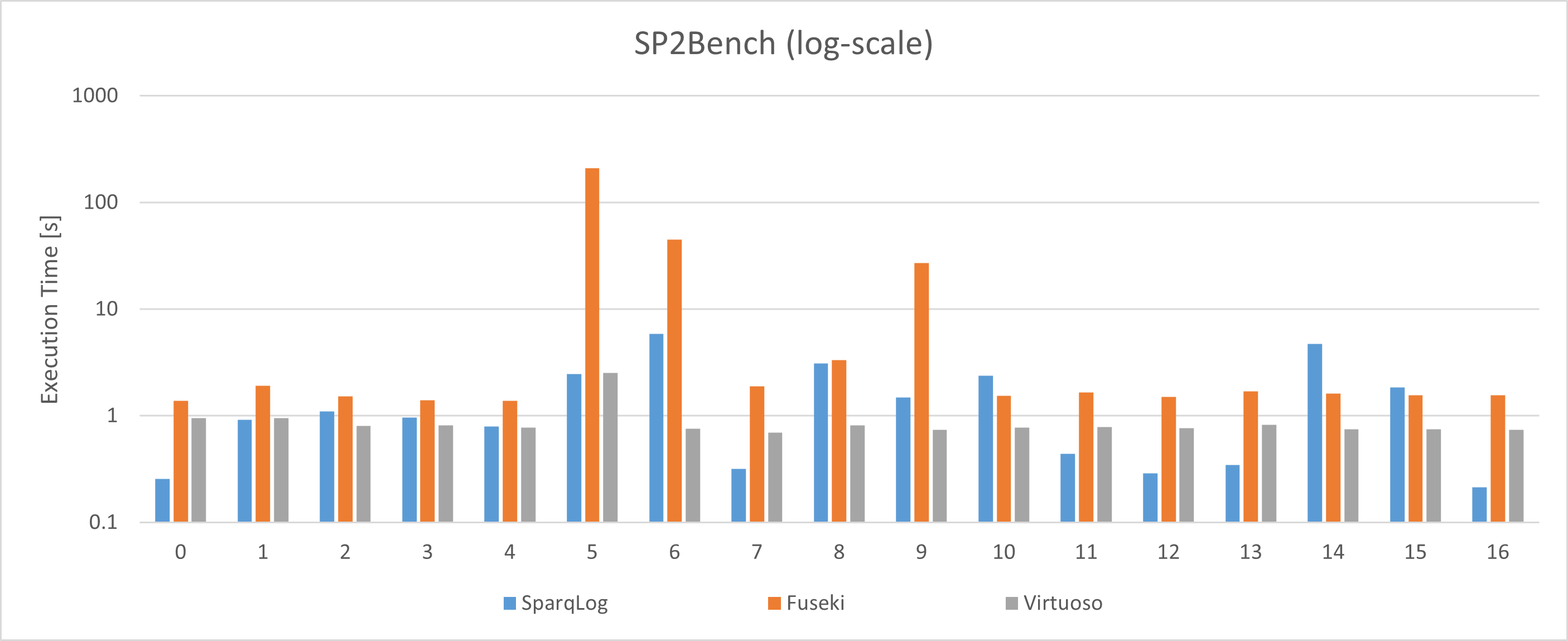
Figure 7. SP2Bench Benchmark (Log Scale)

gMark. Since current SPARQL benchmarks provide only rudimentary coverage of property path expressions, we have evaluated SparqLog, Fuseki, and Virtuoso using the gMark benchmark generator (Bagan et al., 2017), a domain- and language-independent graph instance and query workload generator which specifically focuses on path queries, i.e., queries over property paths. We have evaluated SparqLog’s, Fuseki’s, and Virtuoso’s path query performance on the test and social demo scenarios. Each of these two demo scenarios provides 50 SPARQL queries and a graph instance. Appendix D.3 provides further details on the benchmarks that we used for evaluating a system’s query execution time. Full details on the results can be found in Section D.3 In the following, we compare the results of the three systems on gMark:

Virtuoso could not (correctly) answer $48$ of the in total $100$ queries of the gMark Social and Test benchmark. Thus, it could not correctly answer almost half of the queries provided by both gMark benchmarks, which empirically reveals its dramatic limitations in answering complex property path queries. In $20$ of these $48$ cases, Virtuoso returned an incomplete result. While in solely $3$ incomplete result cases Virtuoso missed solely one tuple in the returned result multi-set, in the remaining $17$ incomplete result cases; Virtuoso produces either the result tuple null or an empty result multi-set instead of the correct non-null/non-empty result multi-set. In the other $28$ cases Virtuoso failed either due to a time-, mem-out or due to not supporting a property path with two variables. This exemplifies severe problems with handling property path queries.

Fuseki suffered on $37$ of the in total $100$ queries of the gMark Social and Test benchmark a time-out (i.e., took longer than $900s$ for answering the queries). Thus, it timed-out on more than a third of gMark queries, which empirically reveals its significant limitations in answering complex property path queries.

SparqLog managed to answer $98$ of gMark’s (in total $100$) queries within less than $200s$ and timed out on solely $2$ queries. The results on the gMark Social benchmark are shown in Figures 8; the results on the gMark Test benchmark are given in Figure 9 in the appendix. These results reveal the strong ability of our system in answering queries that contain complex property paths. Furthermore, each time when both Fuseki and SparqLog returned a result, the results were equal, even further empirically confirming the correctness of our system (i.e., that our system follows the SPARQL standard).

In conclusion, these three benchmarks show that SparqLog (1) is highly competitive with Virtuoso on regular queries with respect to query execution time, (2) follows the SPARQL standard much more accurately than Virtuoso and supports more property path queries than Virtuoso, and (3) dramatically outperforms Fuseki on query execution, while keeping its ability to follow the SPARQL standard accurately.

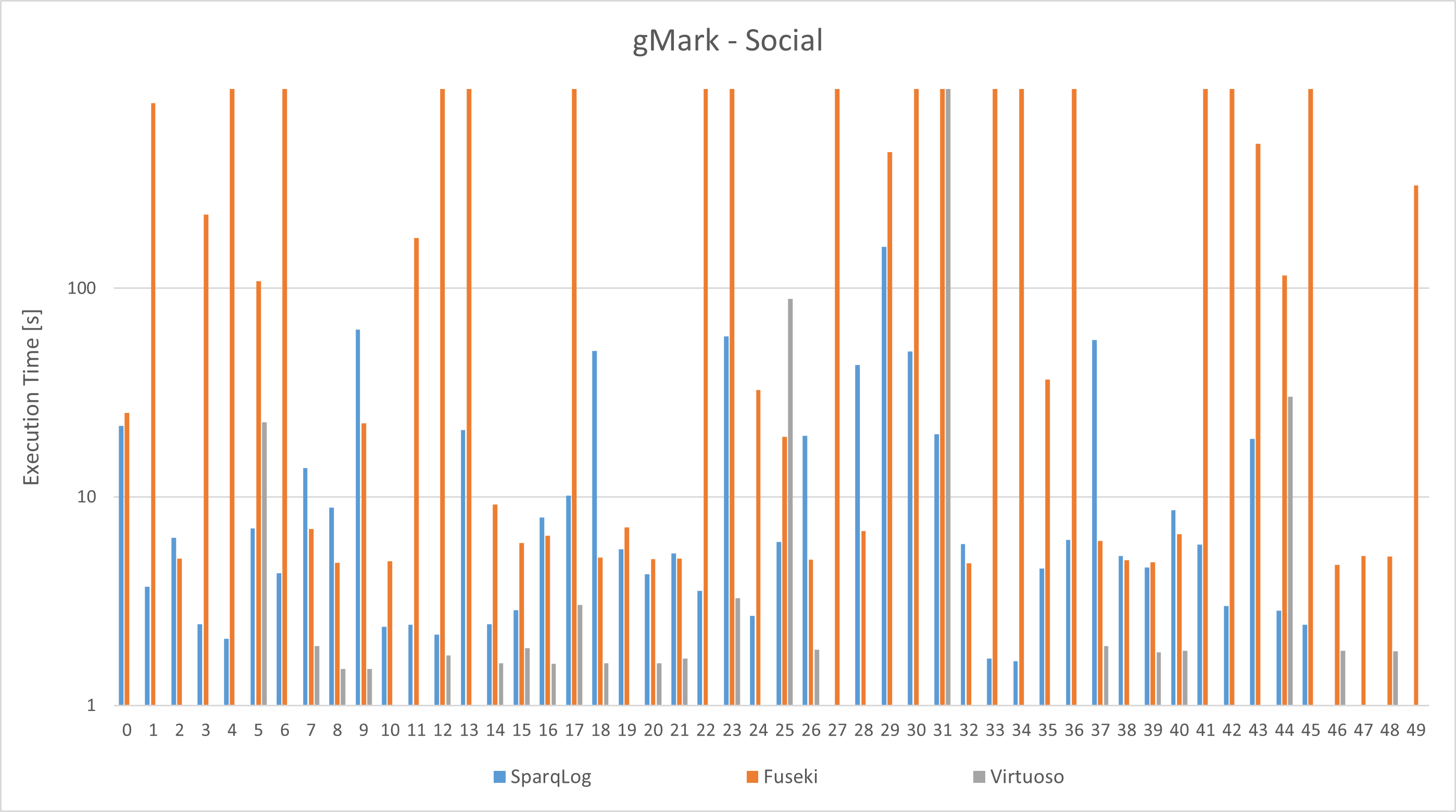
Figure 8. gMark Social Benchmark (Log Scale)

Ontological reasoning

One of the main advantages of our SparqLog system is that it provides a uniform and consistent framework for reasoning and querying Knowledge Graphs. We therefore wanted to measure the performance of query answering in the presence of an ontology. Since Fuseki and Virtuoso do not provide such support, we compare SparqLog with Stardog, which is a commonly accepted state-of-the-art system for reasoning and querying within the Semantic Web. Furthermore, we have created a benchmark based on SP2Bench’s dataset that contains property path queries and ontological concepts such as subPropertyOf and subClassOf and provide this benchmark in the supplementary material.

Figure 10 in Appendix D.8 shows the outcome of these experiments. In summary, we note that SparqLog is faster than Stardog on most queries. Particularly interesting are queries 4 and 5, which contain recursive property path queries with two variables. Our engine needs on query 4 only about a fifth of the execution time of Stardog and it can even answer query 5, on which Stardog times outs (using a timeout of $900s$). On the other queries, Stardog and SparqLog perform similarly.

To conclude, our new SparqLog system does not only follow the SPARQL standard, but it also shows good performance. Even though SparqLog is a full-fledged, general-purpose Knowledge Graph management system and neither a specialized SPARQL engine nor a specialized ontological reasoner, it is highly competitive to state-of-the-art SPARQL engines and reasoners and even outperforms them on answering property path queries and particularly hard cases.

7. Conclusion

In this work we have taken a step towards bringing SPARQL-based systems and Datalog^±-based systems closer together. In particular, we have provided (i) a uniform and fairly complete theoretical translation of SPARQL into Warded Datalog^±, (ii) a practical translation engine that covers most of the SPARQL 1.1 functionality, and (iii) an extensive experimental evaluation.

We note that the contribution of the engine SparqLog we provided in this paper can be seen in two ways: (1) as a stand-alone translation engine for SPARQL into Warded Datalog^±, and (2) as a full Knowledge Graph engine by using our translation engine together with the Vadalog system.

However, our work does not stop here. As next steps, we envisage of course 100% or close to 100% SPARQL coverage. Possibly more (scientifically) interestingly, we plan to expand on the finding that query plan optimization provides a huge effect on performance, and investigate SPARQL-specific query plan optimization in a unified SPARQL-Datalog^± system. Finally, we note that work on a unified benchmark covering all or close to all of the SPARQL 1.1 features would be desirable. As observed in Section 6.1, no such benchmark currently exists.

Appendix

Appendix A Translating SPARQL 1.1 to Warded Datalog^±

In this section, we provide a detailed description of our translation from SPARQL 1.1 to Warded Datalog^±. Note that many of the rules thus generated are simple Datalog rules, i.e., they do not have existentially quantified variables in the head. In such cases, we shall interchangeably refer to these rules as “‘Datalog rules” or “Datalog^± rules”. Of course, if existentially quantified variables are indeed used in the head, we shall always speak of “Datalog^± rules”.

We start with the translation of RDF graphs to Datalog rules in Section A.1. We then detail our translation of graph patterns and the specific translation rules for property path expressions in Sections A.2 and A.3. Finally, in Section A.4, we consider query forms.

A.1. Translation of RDF Graphs

Assume that $I$, $L$ and $B$ are disjoint infinite sets corresponding to IRIs, literals and blank nodes. An RDF term is an element in the set $T=I\cup L\cup B$. An RDF triple is a tuple $(s,p,o)\in T\times I\times T$ where $s$ is called the subject, $p$ is the predicate and $o$ is the object. An RDF graph $G$ is a set of RDF triples. An RDF dataset $D$ is a collection of graphs including a default graph $G_{0}$ and zero or more named graphs, such that a named graph is a pair $(u,G)$ where $u$ is an IRI which identifies the RDF graph $G$.

Let $G$ be a given RDF graph, the translation of the graph to Datalog facts is defined as follows:

1. For each IRI, constant and blank node in $G$ the corresponding facts $iri(X)$, $literal(X)$ and $bnode(X)$ are generated.

2. For each named graph $g$ a tuple $named(g)$ and for each triple $(s,p,o)$ of graph $g$ a fact $triple(s,p,o,g)$ where $g$ is either ”default” for the default graph or the IRI of a named graph is created.

3. A term is either an IRI, a literal or a blank node: The set of terms is represented by the predicate $term$.

Definition A.1 (Terms).

The predicate $terms$ is defined as follows:

$$term(X):- \hskip 4.0ptiri(X).$$

$$term(X):- \hskip 4.0ptliteral(X).$$

$$term(X):- \hskip 4.0ptbnode(X).$$

A.2. Translation of SPARQL Graph Patterns

Assume the existence of an infinite set $V$ of variables disjoint from $T$. We will use $\operatorname{var}(\alpha)$ to denote the set of variables occurring in any structure $\alpha$. A graph pattern is defined recursively as follows: a tuple from $(T\cup V)\times(I\cup V)\times(T\cup V)$ is a triple pattern; if $P_{1}$ and $P_{2}$ are graph patterns, $C$ is a filter constraint, and $g\in I$ then $\{P_{1}\operatorname{{.}}P_{2}\}$, $\{P_{1}\operatorname{UNION}P_{2}\}$, $\{P_{1}\operatorname{OPT}P_{2}\}$, $\{P_{1}\operatorname{MINUS}P_{2}\}$, $\{P_{1}\operatorname{FILTER}C\}$, and; $\{\operatorname{GRAPH}~{}g~{}P_{1}\}$ are graph patterns. A filter constraint is defined recursively as follows: (i) If $?X,?Y\in V$, $c\in I\cup L$ and $r$ is a regular expression then $\operatorname{\emph{true}}$, $\operatorname{\emph{false}}$, $?X=c$, $?X=?Y$, $\operatorname{bound}(?X)$, $\operatorname{isIRI}(?X)$, $\operatorname{isBlank}(?X)$, $\operatorname{isLiteral}(?X)$ and $\operatorname{regex}(?X,r)$ are atomic filter constraints; (ii) If $C_{1}$ and $C_{2}$ are filter constraints then $(!C_{1})$, $(C_{1}~{}\&\&~{}C_{2})$ and $(C_{1}~{}||~{}C_{2})$ are Boolean filter constraints.

A subpattern $P^{\prime}$ of a graph pattern $P$ is defined to be any substring of P that is also a graph pattern. Furthermore $P^{\prime}$ is defined to be an immediate subpattern of $P$ if it is a subpattern of $P$ and if there is no other subpattern of $P$, different from $P$, that contains $P^{\prime}$. A parse tree is specified as a tree $<V,E>$ with the set of nodes $V$ being the subpatterns of a graph pattern $P$ and the set of edges $E$ containing an edge $(P_{1},P_{2})$ if $P_{2}$ is an immediate subpattern of $P_{1}$.

The evaluation of a graph pattern results in a multiset of solution mappings. A solution mapping is a partial function $\mu:V\to T$, i.e. an assignment of variables to RDF terms. The domain of $\mu$, denoted $\operatorname{dom}(\mu)$, is the subset of $V$ where $\mu$ is defined. The empty mapping, denoted $\mu_{0}$, is the mapping satisfying that $\operatorname{dom}(\mu_{0})=\emptyset$. A multiset of solution mappings $\Omega$ is an unsorted list of solution mappings where duplicates are allowed. The domain of $\Omega$ is the set of variables occurring in the solution mappings of $\Omega$.

The notion of compatible mappings is fundamental to evaluating SPARQL graphs patterns. Two mappings $\mu_{1}$ and $\mu_{2}$, are compatible, denoted $\mu_{1}\sim\mu_{2}$, when for all $?X\in\operatorname{dom}(\mu_{1})\cap\operatorname{dom}(\mu_{2})$ it satisfies that $\mu_{1}(?X)=\mu_{2}(?X)$. Note that two mappings with disjoint domains are always compatible, and the empty mapping $\mu_{0}$ is compatible with any other mapping.

Definition A.2 (Compatibility).

The notion of compatible mappings is simulated in Datalog by using the following rules:

$$\mathit{null}("\mathit{null}").$$

$$comp(X,X,X):- \hskip 4.0ptterm(X).$$

$$comp(X,\mathit{Z},X):- \hskip 4.0ptterm(X),\mathit{null}(\mathit{Z}).$$

$$comp(\mathit{Z},X,X):- \hskip 4.0ptterm(X),\mathit{null}(\mathit{Z}).$$

$$comp(\mathit{Z},\mathit{Z},\mathit{Z}):- \hskip 4.0pt\mathit{null}(\mathit{Z}).$$

The predicate $comp(X_{1},X_{2},X_{3})$ describes the compatibility of the values $X_{1}$ and $X_{2}$. The third position $X_{3}$ represents the value, that would be used in the result tuple of a join operation.

A given SPARQL graph pattern is translated into Warded Datalog^± by recursively walking through the parse tree of the query and translating each subpattern into its respective Datalog^± rules (as outlined in (Polleres and Wallner, 2013)). Subpatterns of the parse tree are indexed. The root has index 1, the left child of the $i$-th node has index $2*i$, the right child has index $2*i+1$. During the translation, bindings of the $i$-th subpattern are represented by the predicate $ans_{i}$. Since the order of variables in predicates is relevant, some variable sets will need to be lexicographically ordered, which is denoted by $\overline{x}$ following the notation of (Polleres and Wallner, 2013). $\overline{var}(P)$ shall represent the lexicographically ordered tuple of variables of $P$. Moreover a renaming function $v_{j}:V\rightarrow V$ is defined.

For a given graph pattern $P$ and a given dataset $D=\langle G,G_{named}\rangle$ (where $G$ is the default graph and $G_{named}$ is the set of named graphs) the core translation function $\tau(P,dst,D,\textit{NodeIndex})$ is defined as follows:

1. $P$ is the graph pattern that should be translated next.

2. $dst$ is a Boolean value that describes whether the results should have set semantics ($dst=True$) or bag semantics ($dst=False$).

3. $D$ is the graph on which the query should be evaluated.

4. NodeIndex is the index of the pattern $P$ that should be translated.

In Definitions A.3 to A.11 below, we present the translation function $\tau$ for the various language constructs of graph patterns in SPARQL 1.1.

Definition A.3 (Triple).

Let $P_{i}$ be the i-th subpattern of P and furthermore let $P_{i}$ be a triple pattern $(s,p,o)$, then $\tau(P_{i},\mathit{true},D,i)$ is defined as:

$$ans_{i}(\overline{var}(P_{i}),D):-\hskip 4.0pttriple(s,p,o,D).$$

And $\tau(P_{i},\mathit{false},D,i)$ is defined as:

$$ans_{i}(Id,\overline{var}(P_{i}),D):-\hskip 4.0pttriple(s,p,o,D).$$

Definition A.4 (Graph).

Let $P_{i}$ be the i-th subpattern of P and furthermore let $P_{i}$ be $(\operatorname{GRAPH}$ $g$ $P_{1})$, then $\tau(P_{i},\mathit{true},D,i)$ is defined as:

$$ans_{i}(\overline{var}(P_{i}),D):-\hskip 4.0pt ans_{2i}(\overline{var}(P_{1}),g),$$

$$named(g).$$

$$\tau(P_{1},\mathit{true},g,2i).$$

And $\tau(P_{i},\mathit{false},D,i)$ is defined as:

$$ans_{i}(Id,\overline{var}(P_{i}),D):-\hskip 4.0pt ans_{2i}(Id_{1},\overline{var}(P_{1}),g),$$

$$named(g).$$

$$\tau(P_{1},\mathit{false},g,2i)$$

Definition A.5 (Join).

Let $P_{i}$ be the i-th subpattern of P and furthermore let $P_{i}$ be $(P_{1}\operatorname{{.}}P_{2})$, then $\tau(P_{i},\mathit{true},D,i)$ is defined as:

$$ans_{i}(\overline{x},D):-\hskip 4.0pt ans_{2i}(v_{1}(\overline{var}(P_{1})),D),$$

$$ans_{2i+1}(v_{2}(\overline{var}(P_{2})),D),$$

$$comp(v_{1}(x_{1}),v_{2}(x_{1}),x_{1}),$$

$$\dots,comp(v_{1}(x_{n}),v_{2}(x_{n}),x_{n}).$$

$$\tau(P_{1},\mathit{true},D,2i)$$

$$\tau(P_{2},\mathit{true},D,2i+1)$$

And $\tau(P_{i},\mathit{false},D,i)$ is defined as:

$$ans_{i}(Id,\overline{x},D):-\hskip 4.0pt ans_{2i}(Id_{1},v_{1}(\overline{var}(P_{1})),D),$$

$$ans_{2i+1}(Id_{2},v_{2}(\overline{var}(P_{2})),D),$$

$$comp(v_{1}(x_{1}),v_{2}(x_{1}),x_{1}),$$

$$\dots,comp(v_{1}(x_{n}),v_{2}(x_{n}),x_{n}).$$

$$\tau(P_{1},\mathit{false},D,2i)$$

$$\tau(P_{2},\mathit{false},D,2i+1)$$

with

• $\overline{x}=\overline{var(P_{1})\cup var(P_{2})}$

• $\{x_{1},\dots,x_{n}\}=var(P_{1})\cap var(P_{2})$

• $v_{1},v_{2}:var(P_{1})\cap var(P_{2})\rightarrow V$, such that
  $Image(v_{1})\cap Image(v_{2})=\{\}$

Definition A.6 (Union).

Let $P_{i}$ be the i-th subpattern of P and furthermore let $P_{i}$ be $(P_{1}\operatorname{UNION}P_{2})$, then $\tau(P_{i},\mathit{true},D,i)$ is defined as:

$$ans_{i}(\overline{var}(P_{i}),D):-\hskip 4.0pt ans_{2i}(\overline{var}(P_{1}),D),$$

$$\mathit{null}(x_{1}),\dots\mathit{null}(x_{n}).$$

$$ans_{i}(\overline{var}(P_{i}),D):-\hskip 4.0pt ans_{2i+1}(\overline{var}(P_{2}),D),$$

$$\mathit{null}(y_{1}),\dots\mathit{null}(y_{m}).$$

$$\tau(P_{1},\mathit{true},D,2i)$$

$$\tau(P_{2},\mathit{true},D,2i+1)$$

And $\tau(P_{i},\mathit{false},D,i)$ is defined as:

$$ans_{i}(Id,\overline{var}(P_{i}),D):-\hskip 4.0pt ans_{2i}(Id_{1},\overline{var}(P_{1}),D),$$

$$\mathit{null}(x_{1}),\dots\mathit{null}(x_{n}).$$

$$ans_{i}(Id,\overline{var}(P_{i}),D):-\hskip 4.0pt ans_{2i+1}(Id_{2},\overline{var}(P_{2}),D),$$

$$\mathit{null}(y_{1}),\dots\mathit{null}(y_{m}).$$

$$\tau(P_{1},\mathit{false},D,2i)$$

$$\tau(P_{2},\mathit{false},D,2i+1)$$

with

• $\{x_{1},\dots,x_{n}\}=var(P_{2})\setminus var(P_{1})$

• $\{y_{1},\dots,y_{m}\}=var(P_{1})\setminus var(P_{2})$

Definition A.7 (Optional).

Let $P_{i}$ be the i-th subpattern of P and furthermore let $P_{i}$ be $(P_{1}\operatorname{OPT}P_{2})$, then $\tau(P_{i},\mathit{true},D,i)$ is defined as:

$$ans_{opt-i}(\overline{var}(P_{1}),D):-\hskip 4.0pt ans_{2i}(\overline{var}(P_{1}),D),$$

$$ans_{2i+1}(v_{2}(\overline{var}(P_{2})),D),$$

$$comp(x_{1},v_{2}(x_{1}),z_{1}),$$

$$\dots,comp(x_{n},v_{2}(x_{n}),z_{n}).$$

$$ans_{i}(\overline{var}(P_{i}),D):-\hskip 4.0pt ans_{2i}(v_{1}(\overline{var}(P_{1})),D),$$

$$ans_{2i+1}(v_{2}(\overline{var}(P_{2})),D),$$

$$comp(v_{1}(x_{1}),v_{2}(x_{1}),x_{1}),$$

$$\dots,comp(v_{1}(x_{n}),v_{2}(x_{n}),x_{n}).$$

$$ans_{i}(\overline{var}(P_{i}),D):-\hskip 4.0pt ans_{2i}(\overline{var}(P_{1}),D),$$

$$not\hskip 4.0ptans_{opt-i}(\overline{var}(P_{1}),D),$$

$$\mathit{null}(y_{1}),\dots,\mathit{null}(y_{m}).$$

$$\tau(P_{1},\mathit{true},D,2i)$$

$$\tau(P_{2},\mathit{true},D,2i+1)$$

And $\tau(P_{i},\mathit{false},D,i)$ is defined as:

$$ans_{opt-i}(\overline{var}(P_{1}),D):-\hskip 4.0pt ans_{2i}(Id_{1},\overline{var}(P_{1}),D),$$

$$ans_{2i+1}(Id_{2},v_{2}(\overline{var}(P_{2})),D),$$

$$comp(x_{1},v_{2}(x_{1}),z_{1}),$$

$$\dots,comp(x_{n},v_{2}(x_{n}),z_{n}).$$

$$ans_{i}(Id,\overline{var}(P_{i}),D):-\hskip 4.0pt ans_{2i}(Id_{1},v_{1}(\overline{var}(P_{1})),D),$$

$$ans_{2i+1}(Id_{2},v_{2}(\overline{var}(P_{2})),D),$$

$$comp(v_{1}(x_{1}),v_{2}(x_{1}),x_{1}),$$

$$\dots,comp(v_{1}(x_{n}),v_{2}(x_{n}),x_{n}).$$

$$ans_{i}(Id,\overline{var}(P_{i}),D):-\hskip 4.0pt ans_{2i}(Id_{1},\overline{var}(P_{1}),D),$$

$$not\hskip 4.0ptans_{opt-i}(\overline{var}(P_{1}),D),$$

$$\mathit{null}(y_{1}),\dots,\mathit{null}(y_{m}).$$

$$\tau(P_{1},\mathit{false},D,2i)$$

$$\tau(P_{2},\mathit{false},D,2i+1)$$

with

• $\overline{var}(P_{i})=\overline{var(P_{1})\cup var(P_{2})}$

• $\{x_{1},\dots,x_{n}\}=var(P_{1})\cap var(P_{2})$

• $\{y_{1},\dots,y_{m}\}=var(P_{2})\setminus var(P_{1})$

• $v_{1},v_{2}:var(P_{1})\cap var(P_{2})\rightarrow V$, such that
  $Image(v_{1})\cap Image(v_{2})=\{\}$

Definition A.8 (Filter).

Let $P_{i}$ be the i-th subpattern of P and furthermore let $P_{i}$ be $(P_{1}\operatorname{FILTER}C)$, then $\tau(P_{i},\mathit{true},D,i)$ is defined as:

$$ans_{i}(\overline{var}(P_{i}),D):-\hskip 4.0pt ans_{2i}(\overline{var}(P_{1}),D),C.$$

$$\tau(P_{1},\mathit{true},D,2i)$$

And $\tau(P_{i},\mathit{false},D,i)$ is defined as:

$$ans_{i}(Id,\overline{var}(P_{i}),D):-\hskip 4.0pt ans_{2i}(Id_{1},\overline{var}(P_{1}),D),C.$$

$$\tau(P_{1},\mathit{false},D,2i)$$

Definition A.9 (Optional Filter).

Let $P_{i}$ be the i-th subpattern of P and furthermore let $P_{i}$ be $(P_{1}\operatorname{OPT}(P_{2}\operatorname{FILTER}C))$, then $\tau(P_{i},\mathit{true},D,i)$ is defined as:

$$ans_{opt-i}(\overline{var}(P_{1}),D):-\hskip 4.0pt ans_{2i}(\overline{var}(P_{1}),D),$$

$$ans_{2i+1}(v_{2}(\overline{var}(P_{2})),D),$$

$$comp(x_{1},v_{2}(x_{1}),z_{1}),$$

$$\dots,comp(x_{n},v_{2}(x_{n}),z_{n}),C.$$

$$ans_{i}(\overline{var}(P_{i}),D):-\hskip 4.0pt ans_{2i}(v_{1}(\overline{var}(P_{1})),D),$$

$$ans_{2i+1}(v_{2}(\overline{var}(P_{2})),D),$$

$$comp(v_{1}(x_{1}),v_{2}(x_{1}),x_{1}),$$

$$\dots,comp(v_{1}(x_{n}),v_{2}(x_{n}),x_{n}),C.$$

$$ans_{i}(\overline{var}(P_{i}),D):-\hskip 4.0pt ans_{2i}(\overline{var}(P_{1}),D),$$

$$not\hskip 4.0ptans_{opt-i}(\overline{var}(P_{1}),D),$$

$$\mathit{null}(y_{1}),\dots,\mathit{null}(y_{m}).$$

$$\tau(P_{1},\mathit{true},D,2i)$$

$$\tau(P_{2},\mathit{true},D,2i+1)$$

And $\tau(P_{i},\mathit{false},D,i)$ is defined as:

$$ans_{opt-i}(\overline{var}(P_{1}),D):-\hskip 4.0pt ans_{2i}(Id_{1},\overline{var}(P_{1}),D),$$

$$ans_{2i+1}(Id_{2},v_{2}(\overline{var}(P_{2})),D),$$

$$comp(x_{1},v_{2}(x_{1}),z_{1}),$$

$$\dots,comp(x_{n},v_{2}(x_{n}),z_{n}),C.$$

$$ans_{i}(Id,\overline{var}(P_{i}),D):-\hskip 4.0pt ans_{2i}(Id_{1},v_{1}(\overline{var}(P_{1})),D),$$

$$ans_{2i+1}(Id_{2},v_{2}(\overline{var}(P_{2})),D),$$

$$comp(v_{1}(x_{1}),v_{2}(x_{1}),x_{1}),$$

$$\dots,comp(v_{1}(x_{n}),v_{2}(x_{n}),x_{n}),C.$$

$$ans_{i}(Id,\overline{var}(P_{i}),D):-\hskip 4.0pt ans_{2i}(Id_{1},\overline{var}(P_{1}),D),$$

$$not\hskip 4.0ptans_{opt-i}(\overline{var}(P_{1}),D),$$

$$\mathit{null}(y_{1}),\dots,\mathit{null}(y_{m}).$$

$$\tau(P_{1},\mathit{false},D,2i)$$

$$\tau(P_{2},\mathit{false},D,2i+1)$$

with

• $\overline{var}(P_{i})=\overline{var(P_{1})\cup var(P_{2})}$

• $\{x_{1},\dots,x_{n}\}=var(P_{1})\cap var(P_{2})$

• $\{y_{1},\dots,y_{m}\}=var(P_{2})\setminus var(P_{1})$

• $v_{1},v_{2}:var(P_{1})\cap var(P_{2})\rightarrow V$, such that
  $Image(v_{1})\cap Image(v_{2})=\{\}$

Definition A.10 (Minus).

Let $P_{i}$ be the i-th subpattern of P and furthermore let $P_{i}$ be $(P_{1}\operatorname{MINUS}P_{2})$, then $\tau(P_{i},\mathit{true},D,i)$ is defined as:

$$ans_{join-i}(\overline{x},D):-\hskip 4.0pt ans_{2i}(\overline{var}(P_{1}),D),$$

$$ans_{2i+1}(v_{2}(\overline{var}(P_{2})),D),$$

$$comp(x_{1},v_{2}(x_{1}),z_{1}),$$

$$\dots,comp(x_{n},v_{2}(x_{n}),z_{n}).$$

$$ans_{equal-i}(\overline{var}(P_{1}),D):-\hskip 4.0pt ans_{join-i}(\overline{x},D),$$

$$x_{1}=v_{2}(x_{1}),\hskip 3.0ptnot\hskip 4.0ptnull(x_{1}).$$

$$\dots$$

$$ans_{equal-i}(\overline{var}(P_{1}),D):-\hskip 4.0pt ans_{join-i}(\overline{x},D),$$

$$x_{n}=v_{2}(x_{n}),\hskip 3.0ptnot\hskip 4.0ptnull(x_{n}).$$

$$ans_{i}(\overline{var}(P_{1}),D):-\hskip 4.0pt ans_{2i}(\overline{var}(P_{1}),D),$$

$$not\hskip 4.0ptans_{equal-i}(\overline{var}(P_{1}),D).$$

$$\tau(P_{1},\mathit{true},D,2i)$$

$$\tau(P_{2},\mathit{true},D,2i+1)$$

And $\tau(P_{i},\mathit{false},D,i)$ is defined as:

$$ans_{join-i}(\overline{x},D):-\hskip 4.0pt ans_{2i}(Id_{1},\overline{var}(P_{1}),D),$$

$$ans_{2i+1}(Id_{2},v_{2}(\overline{var}(P_{2})),D),$$

$$comp(x_{1},v_{2}(x_{1}),z_{1}),$$

$$\dots,comp(x_{n},v_{2}(x_{n}),z_{n}).$$

$$ans_{equal-i}(\overline{var}(P_{1}),D):-\hskip 4.0pt ans_{join-i}(\overline{x},D),$$

$$x_{1}=v_{2}(x_{1}),\hskip 3.0ptnot\hskip 4.0ptnull(x_{1}).$$

$$\dots$$

$$ans_{equal-i}(\overline{var}(P_{1}),D):-\hskip 4.0pt ans_{join-i}(\overline{x},D),$$

$$x_{n}=v_{2}(x_{n}),\hskip 3.0ptnot\hskip 4.0ptnull(x_{n}).$$

$$ans_{i}(Id,\overline{var}(P_{1}),D):-\hskip 4.0pt ans_{2i}(Id_{1},\overline{var}(P_{1}),D),$$

$$not\hskip 4.0ptans_{equal-i}(\overline{var}(P_{1}),D).$$

$$\tau(P_{1},\mathit{false},D,2i)$$

$$\tau(P_{2},\mathit{false},D,2i+1)$$

with

• $\overline{x}=\overline{var(P_{1})\cup v_{2}(var(P_{2}))}$

• $\{x_{1},\dots,x_{n}\}=var(P_{1})\cap var(P_{2})$

• $v_{2}:var(P_{1})\cap var(P_{2})\rightarrow V\setminus var(P_{1})$

Property path patterns are given in the form $S\hskip 4.0ptP_{1}\hskip 4.0ptO$, where $P_{1}$ is a property path expression. Due to the complex semantics of property paths, we have introduced a separate translation function $\tau_{PP}$ for property path expressions, which we will take a closer look at in Section A.3.

Definition A.11 (Property Path Pattern).

Let $P_{i}$ be the i-th subpattern of $P$ and furthermore let $P_{i}=S\hskip 4.0ptP_{1}\hskip 4.0ptO$ be a property path pattern, then $\tau(P_{i},\mathit{true},D,i)$ is defined as:

$$ans_{i}(\overline{var}(P_{i}),D):-\hskip 4.0pt ans_{2i}(S,O,D).$$

$$\tau_{PP}(P_{1},\mathit{true},S,O,D,2i)$$

And $\tau(P_{i},\mathit{false},D,i)$ is defined as:

$$ans_{i}(Id,\overline{var}(P_{i}),D):-\hskip 4.0pt ans_{2i}(Id_{1},S,O,D).$$

$$\tau_{PP}(P_{1},\mathit{false},S,O,D,2i)$$

with $\tau_{PP}$ being the translation function for property path expressions defined next.

A.3. Translation of Property Path Expressions

A property path expression (or, simply, a path expression) is defined recursively as follows:

• if $a\in I$, then $a$ is a link path expression;

• If $PP_{1}$ and $PP_{2}$ are property path expressions then

  • $^PP_{1}$ is an inverse path expression;

  • $PP_{1}\mid PP_{2}$ is an alternative path expression;

  • $PP_{1}/PP_{2}$ is a sequence path expression;

  • $PP_{1}?$ is a zero-or-one path expression;

  • $PP_{1}+$ is a one-or-more path expression;

  • $PP_{1}*$ is a zero-or-more path expression;

• if $\mathcal{P}$ is a set of link path expressions $p_{i}$ and inverse link path expressions $^p_{j}$, then $!\mathcal{P}$ is a negated path expression.

A property path pattern is a tuple $t$ of the form $(u,p,v)$, where $u,v\in(I\cup V)$ and $p$ is a property path expression. Analogously to our translation function $\tau(P,dst,D,\textit{NodeIndex})$ for SPARQL patterns, we define a translation function $\tau_{PP}(PP,dst,S,O,D,\textit{NodeIndex})$ for property path expressions, where $S,O$, are the subject and object of the top-level property path expression that have to be kept track of during the entire evaluation.

In the following we will only state the translations for property path expressions under bag semantics (i.e. $dst=false$), since for set semantics the IDs are simply left out or set to a constant value (e.g. $Id=[]$).

Definition A.12 (Link Property Path).

Let $PP_{i}$ be the $i$-th subexpression of a property path expression $PP$ and furthermore let $PP_{i}=p_{1}$ be a link property path expression. Then $\tau_{PP}(PP_{i},\mathit{false},S,O,D,i)$ is defined as:

$$ans_{i}(Id,X,Y,D):-\hskip 4.0pt triple(X,p1,Y,D).$$

Definition A.13 (Inverse Property Path).

Let $PP_{i}$ be the $i$-th subexpression of a property path expression $PP$ and furthermore let $PP_{i}=^PP_{1}$ be an inverse property path expression. Then $\tau_{PP}(PP_{i},\mathit{false}$, $S,O,D,i)$ is defined as:

$$ans_{i}(Id,X,Y,D):-\hskip 4.0pt ans_{2i}(Id_{1},Y,X,D).$$

$$\tau_{PP}(PP_{1},\mathit{false},S,O,D,2i)$$

Definition A.14 (Alternative Property Path).

Let $PP_{i}$ be the $i$-th subexpression of a property path expression $PP$ and furthermore let $PP_{i}=PP_{1}|PP_{2}$ be a alternative property path expression. Then $\tau_{PP}(PP_{i},\mathit{false},S,O,D,i)$ is defined as:

$$ans_{i}(Id,X,Y,D):-\hskip 4.0pt ans_{2i}(Id_{1},X,Y,D).$$

$$ans_{i}(Id,X,Y,D):-\hskip 4.0pt ans_{2i+1}(Id_{1},X,Y,D).$$

$$\tau_{PP}(PP_{1},\mathit{false},S,O,D,2i)$$

$$\tau_{PP}(PP_{2},\mathit{false},S,O,D,2i+1)$$

Definition A.15 (Sequence Property Path).

Let $PP_{i}$ be the $i$-th subexpression of a property path expression $PP$ and furthermore let $PP_{i}=PP_{1}/PP_{2}$ be a sequence property path expression. Then $\tau_{PP}(PP_{i}$, $\mathit{false},S,O,D,i)$ is defined as:

$$ans_{i}(Id,X,Z,D):-\hskip 4.0pt ans_{2i}(Id_{1},X,Y,D),$$

$$ans_{2i+1}(Id_{2},Y,Z,D).$$

$$\tau_{PP}(PP_{1},\mathit{false},S,O,D,2i)$$

$$\tau_{PP}(PP_{2},\mathit{false},S,O,D,2i+1)$$

Definition A.16 (One-Or-More Property Path).

Let $PP_{i}$ be the $i$-th subexpression of a property path expression $PP$ and furthermore let $PP_{i}=PP_{1}+$ be a one-or-more property path expression. Then $\tau_{PP}(PP_{i},\mathit{false},S,O,D,i)$ is defined as:

$$ans_{i}(Id,X,Y,D):-\hskip 4.0pt ans_{2i}(Id_{1},X,Y,D),Id=[].$$

$$ans_{i}(Id,X,Z,D):-\hskip 4.0pt ans_{2i}(Id_{1},X,Y,D),$$

$$ans_{i}(Id_{2},Y,Z,D),Id=[].$$

$$\tau_{PP}(PP_{1},\mathit{false},S,O,D,2i)$$

Definition A.17 (SubjectOrObject).

The subjectOrObject predicate defines intuitively the set of all possible subjects and objects occurring in a graph, i.e.:

$$subjectOrObject(X):-\hskip 4.0pt triple(X,P,Y,D).$$

$$subjectOrObject(Y):-\hskip 4.0pt triple(X,P,Y,D).$$

Definition A.18 (Zero-Or-One Property Path).

Let $PP_{i}$ be the $i$-th subexpression of a property path expression $PP$ and furthermore let $PP_{i}=PP_{1}?$ be a zero-or-one property property path expression. Then $\tau_{PP}(PP_{i},\mathit{false},S,O,D,i)$ consists of the following rules:

$$ans_{i}(Id,X,X,D):-\hskip 4.0pt subjectOrObject(X),Id=[].$$

$$ans_{i}(Id,X,Y,D):-\hskip 4.0pt ans_{2i}(Id_{1},X,Y,D),Id=[].$$

$$\tau_{PP}(PP_{1},\mathit{false},S,O,D,2i)$$

Moreover, if either one of $S$ and $O$ is a variable and the other is a non-variable $t$ or both $S$ and $O$ are the same non-variable $t$, then the following rule is added:

$$ans_{i}(Id,X,X,D):-\hskip 4.0pt not\hskip 4.0ptTerm(X),X=t,Id=[].$$

It should be noted that, according to the SPARQL semantics of property paths, zero-or-one, zero-or-more, and one-or-more property paths always have set semantics. This is why the Datalog^± rules for these three path expressions contain a body literal $Id=[]$. By forcing the tuple ID to the same value whenever one of these rules fires, multiply derived tuples are indistinguishable for our system and will, therefore, never give rise to duplicates.

Definition A.19 (Zero-Or-More Property Path).

Let $PP_{i}$ be the $i$-th subexpression of a property path expression $PP$ and furthermore let $PP_{i}=PP_{1}*$ be a zero-or-more property property path expression. Then $\tau_{PP}(PP_{i},\mathit{false},S,O,D,i)$ consists of the following rules:

$$ans_{i}(Id,X,X,D):-\hskip 4.0pt subjectOrObject(X),Id=[].$$

$$ans_{i}(Id,X,Y,D):-\hskip 4.0pt ans_{2i}(Id_{1},X,Y,D),Id=[].$$

$$ans_{i}(Id,X,Z,D):-\hskip 4.0pt ans_{2i}(Id_{1},X,Y,D),$$

$$ans_{i}(Id_{2},Y,Z,D),Id=[].$$

$$\tau_{PP}(PP_{1},\mathit{false},S,O,D,2i)$$

Moreover, if either one of $S$ and $O$ is a variable and the other is a non-variable $t$ or both $S$ and $O$ are the same non-variable $t$, then the following rule is added:

$$ans_{i}(Id,X,X,D):-\hskip 4.0pt not\hskip 4.0ptTerm(X),X=t,Id=[].$$

Essentially, the zero-or-more property path is a combination of the zero-or-one and one-or-more property path.

Definition A.20 (Negated Property Path).

Let $PP_{i}$ be the $i$-th subexpression of a property path expression $PP$ and furthermore let $PP_{i}=!(\mathcal{P})$ be a negated property path expression. Then $\tau_{PP}(PP_{i}$, $\mathit{false},S,O,D,i)$ is defined as:

$$ans_{i}(Id,X,Y,D):-\hskip 4.0pt triple(X,P,Y,D),P!=p_{f_{1}},\dots,P!=p_{f_{n}}.$$

$$ans_{i}(Id,Y,X,D):-\hskip 4.0pt triple(X,P,Y,D),P!=p_{b_{1}},\dots,P!=p_{b_{m}}.$$

with

• $p_{f_{1}},\dots,p_{f_{n}}\in\{p|p\in\mathcal{P}\}$ … i.e. the set of negated forward predicates.

• $p_{b_{1}},\dots,p_{b_{m}}\in\{p|^p\in\mathcal{P}\}$ … i.e. the set of negated backward predicates.

A.4. Translation of Query Forms

Let $P_{1}$ be a graph pattern and $W$ be a set of variables. We consider two types of query forms: $(\operatorname{SELECT}$ $W$ $P_{1})$ and $(\operatorname{ASK}P_{1})$. Their translation is given below.

Definition A.21 (Select).

Let $P_{i}$ be the i-th subpattern of P and furthermore let $P_{i}$ be $(\operatorname{SELECT}$ $W$ $P_{1})$, then $\tau(P_{i},\mathit{true},D,i)$ is defined as:

$$ans_{i}(\overline{var}(W),D):-\hskip 4.0pt ans_{2i}(\overline{var}(P_{1}),D).$$

$$\tau(P_{1},\mathit{true},D,2i)$$

And $\tau(P_{i},\mathit{false},D,i)$ is defined as:

$$ans_{i}(Id,\overline{var}(W),D):-\hskip 4.0pt ans_{2i}(Id_{1},\overline{var}(P_{1}),D).$$

$$\tau(P_{1},\mathit{false},D,2i)$$

Definition A.22 (Ask).

Let $P_{i}$ be the i-th subpattern of P and furthermore let $P_{i}$ be $\operatorname{ASK}P_{1})$, then $\tau(P_{i},\mathit{true},D,i)$ is defined as:

$$ans_{i}(HasResult):-\hskip 4.0pt ans\_ask_{i}(HasResult).$$

$$ans_{i}(HasResult):-\hskip 4.0pt not\hskip 4.0ptans\_ask_{i}(True),HasResult=false.$$

$$ans\_ask_{i}(HasResult):-\hskip 4.0pt ans_{2i}(\overline{var}(P_{1}),D),HasResult=true.$$

$$\tau(P_{1},\mathit{true},D,2i)$$

And $\tau(P_{i},\mathit{false},D,i)$ is defined as:

$$ans_{i}(HasResult):-\hskip 4.0pt ans\_ask_{i}(HasResult).$$

$$ans_{i}(HasResult):-\hskip 4.0pt not\hskip 4.0ptans\_ask_{i}(True),HasResult=false.$$

$$ans\_ask_{i}(HasResult):-\hskip 4.0pt ans_{2i}(Id_{1},\overline{var}(P_{1}),D),HasResult=true.$$

$$\tau(P_{1},\mathit{false},D,2i)$$

Appendix B Correctness of the Translation

As was mentioned in Section 5.3, we have applied a two-way strategy for ensuring the correctness of our translation from SPARQL 1.1 to Warded Datalog^± by carrying out an extensive empirical evaluation and a formal analysis. For the empirical evaluation, we have run our SparqLog system as well as Fuseki and Virtuoso on several benchmarks which provide a good coverage of SPARQL 1.1. The results of our empirical evaluation are summarized in Section 6.2. They give strong evidence for the correctness of the translation applied by SparqLog. To provide yet further evidence, we will now formally examine the Warded Datalog^± rules produced by our translation for the various SPARQL language constructs and compare them with the formal semantics of these language constructs.

As was mentioned in Section 4, SparqLog includes a translation engine with three methods, namely a data translation method, a query translation method, and a solution translation method. The data translation is very straightforward. In particular, the IRIs, literals and blank nodes as well as the triples in an RDF graph are presented as Datalog ground facts in the obvious way. Recall from Table 1 that, as far as query forms are concerned, we currently only support SELECT (which is by far the most common one) and ASK. The former allows one to define a projection to some of the variables in the graph pattern while the latter just asks if at least some mapping satisfying the graph pattern exists. In case of SELECT, the solution modifier can be further extended by a DISTINCT, ORDER BY, LIMIT, or OFFSET clause. The two supported solution modifiers (with the possible extensions) are obvious and they are taken care of by the solution translation method of SparqLog. In the sequel, we therefore restrict our discussion to the query translation method. As in Section 5, we treat the basic translation rules and the translation of property paths in separate subsections.

B.1. Basic Translation Rules

First we recall some basic principles of defining a formal semantics of SPARQL (Angles and Gutiérrez, 2008; Arenas et al., 2009; Polleres and Wallner, 2013). At the heart of evaluating a SPARQL query is the evaluation of the graph pattern (GP) given in the WHERE clause of the query. This evaluation is relative to the active graph $D$, which is initially the default graph (obtained by merging the graphs given in the FROM clause of the query) and which can be switched to some named graph (given by an IRI in a FROM NAMED clause of the query) via the GRAPH construct. We write $\operatorname{gr}(u)$ to denote the graph with name $u$ and we write $\mathit{names}$ to denote all names of named graphs according to the FROM NAMED clauses.

The result of evaluating a graph pattern $P$ relative to some graph $D$, denoted by $\llbracket P\rrbracket_{D}$, is a multiset of partial mappings $\mu\colon V\rightarrow T$ (simply referred to as “mappings” henceforth), where $V$ is the set of variables and $T$ is the set of terms (i.e., the union of IRIs, blank nodes and literals). It is convenient to allow also the constant “null” as function value to indicate by $\mu(?X)=$ “null” that $\mu$ is undefined on variable $?X$. The domain of $\mu$, denoted $\operatorname{dom}(\mu)$, is defined as the set of variables on which $\mu$ is defined. Mappings are applied to triple patterns in the obvious way, i.e., let $t=(s,p,o)$ be a triple pattern and let $\operatorname{var}(t)$ denote the variables in $t$. For a mapping $\mu$ with $\operatorname{var}(t)\subseteq\operatorname{dom}(\mu)$, we write $\mu(t)$ to denote the triple obtained by replacing each variable $?X\in\operatorname{var}(t)$ by $\mu(?X)$.

Compatibility. An important property when combining or comparing two mappings is compatibility. Two mappings $\mu_{1},\mu_{2}$ are compatible, denoted $\mu_{1}\sim\mu_{2}$, if $\mu_{1}(?X)=\mu_{2}(?X)$ holds for all $?X\in\operatorname{dom}(\mu_{1})\cap\operatorname{dom}(\mu_{2})$. In this case, the mapping $\mu=\mu_{1}\cup\mu_{2}$ with $\mu(?X)=\mu_{1}(?X)$ if $?X\in\operatorname{dom}(\mu_{1})$ and $\mu(?X)=\mu_{2}(?X)$ if $?X\in\operatorname{dom}(\mu_{2})$ is well-defined.

In Section A.2, we have also defined the compatibility of two individual terms or nulls $v_{1},v_{2}$, namely: $v_{1}$ and $v_{2}$ are compatible if they are equal (i.e., either the same term or both ‘null”) or if one of them is “null”. Clearly, two partial mappings $\mu_{1},\mu_{2}$ are compatible if and only if $\mu_{1}(?X)$ and $\mu_{2}(?X)$ are compatible for every variable $?X\in\operatorname{var}(\mu_{1})\cap\operatorname{var}(\mu_{2})$. If this is the case, then $\mu=\mu_{1}\cup\mu_{2}$ is obtained as follows: for every variable $?X$, (1) if $\mu_{1}(?X)=\mu_{2}(?X)$ (where $\mu_{1}(?X)$ and $\mu_{2}(?X)$ are either the same term or they are both “null”), then $\mu(?X)=\mu_{1}(?X)=\mu_{2}(?X)$; and (2) if one of $\mu_{1}(?X),\mu_{2}(?X)$ is a term and the other is “null”, then $\mu(?X)$ is set equal to the term.

We observe that the auxiliary predicate $comp(X_{1},X_{2},X_{3})$ defined in Section A.2 realises precisely the compatibility check between two values $\mu_{1}(?X)$ and $\mu_{2}(?X)$ (in the first two components of $comp$) and yields $\mu(?X)$ in the third component.

Operations on multisets of mappings. We consider the following operations between two sets of mappings $\Omega_{1},\Omega_{2}$:

$\Omega_{1}\Join\Omega_{2}=\{\hskip-2.0pt\{\mu_{1}\cup\mu_{2}\mid\mu_{1}\in\Omega_{1},\mu_{2}\in\Omega_{2}\text{ and }\mu_{1}\sim\mu_{2}\}\hskip-2.0pt\}$

$\Omega_{1}\cup\Omega_{2}=\{\hskip-2.0pt\{\mu\mid\mu\in\Omega_{1}\textrm{ or }\mu\in\Omega_{2}\}\hskip-2.0pt\}$

$\Omega_{1}\setminus\Omega_{2}=\{\hskip-2.0pt\{\mu_{1}\in\Omega_{1}\mid\textrm{ for all }\mu_{2}\in\Omega_{2},\mu_{1}\not\sim\mu_{2}\}\hskip-2.0pt\}$

$\Omega_{1}\sqsupset\hskip-1.7pt\Join\Omega_{2}=(\Omega_{1}\Join\Omega_{2})\cup(\Omega_{1}\setminus\Omega_{2})$

Note that, of the above operations, only the union $\cup$ may alter the cardinality of elements in the resulting multiset, namely: if a mapping $\mu$ is contained in both $\Omega_{1}$ and $\Omega_{2}$, then its cardinality in $\Omega$ is the sum of the original cardinalities in $\Omega_{1}$ and $\Omega_{2}$.

Semantics of basic SPARQL constructs. The semantics $\llbracket P\rrbracket_{D}$ of a graph pattern $P$ is defined recursively on the structure of $P$. In the base case, $P$ is a triple pattern $P=(s,p,o)$ and $\llbracket P\rrbracket_{D}$ is defined as $\llbracket P\rrbracket_{D}=\{\mu\mid\operatorname{dom}(\mu)=\operatorname{var}(P)$ and $\mu(P)\in D\}$. For complex graph patterns $P$, the semantics definition $\llbracket P\rrbracket_{D}$ is shown in Table 4.

Table 4. Semantics of basic graph patterns. $P_{1},P_{2}$ are graph patterns, $C$ is a filter constraint, $u\in I$ and $?X\in V$.

Graph pattern $P$	Evaluation $\llbracket P\rrbracket_{D}$
$(\operatorname{GRAPH}\,u\,P_{1})$	$\llbracket P_{1}\rrbracket_{\operatorname{gr}(u)}$ if $u\in\mathit{names}$ and $\emptyset$ otherwise
$(\operatorname{GRAPH}\,?X\,P_{1})$	$\bigcup_{v\in\mathit{names}}(\llbracket P_{1}\rrbracket_{\operatorname{gr}(v)}\Join\{?X\to v\})$
$(P_{1}\operatorname{{.}}P_{2})$	$\llbracket P_{1}\rrbracket_{D}\Join\llbracket P_{2}\rrbracket_{D}$
$(P_{1}\operatorname{FILTER}C)$	$\{\mu\mid\mu\in\llbracket P_{1}\rrbracket_{D}\text{ and }\mu\models C\}$
$(P_{1}\operatorname{OPT}P_{2})$	$\llbracket P_{1}\rrbracket_{D}\sqsupset\hskip-1.7pt\Join\llbracket P_{2}\rrbracket_{D}$
$(P_{1}\operatorname{OPT}$	$\{\hskip-2.0pt\{\mu\mid\mu\in\llbracket P_{1}\rrbracket_{D}\bowtie\llbracket P_{2}\rrbracket_{D}\text{ and }\mu\models C\}\hskip-2.0pt\}$ $\cup$
$(P_{2}\operatorname{FILTER}C))$	$\{\hskip-2.0pt\{\mu_{1}\mid\mu_{1}\in\llbracket P_{1}\rrbracket_{D}\text{ and for all }\mu_{2}\in\llbracket P_{2}\rrbracket_{D}$:
	either $\mu_{1}\not\sim\mu_{2}$
	or $\mu_{1}\sim\mu_{2}$ and $\mu_{1}\cup\mu_{2}\not\models C\}\hskip-2.0pt\}$
$(P_{1}\operatorname{UNION}P_{2})$	$\llbracket P_{1}\rrbracket_{D}\cup\llbracket P_{2}\rrbracket_{D}$
$(P_{1}\operatorname{MINUS}P_{2})$	$\{\hskip-2.0pt\{\mu_{1}\in\llbracket P_{1}\rrbracket_{D}\mid\textrm{ for all }\mu_{2}\in\llbracket P_{2}\rrbracket_{D}$,
	$(\mu_{1}\not\sim\mu_{2}\text{ or }\operatorname{dom}(\mu_{1})\cap\operatorname{dom}(\mu_{2})=\emptyset)\}\hskip-2.0pt\}$

Translation of basic SPARQL constructs. We are now ready to inspect the translations from SPARQL 1.1 to Warded Datalog^± given in Figure 5 and Section A.2. As in Section 5.1, we concentrate on bag semantics as the more complex case.

Triple. First consider the base case of graph patterns, namely a triple pattern $P_{i}=(s,p,o)$, where each of $s,p,o$ can be a term or a variable. Clearly, the single rule produced by our translation $\tau(P_{i},\mathit{false},D,i)$ in Definition A.3 produces all mappings in $\operatorname{var}(P_{i})$ that match $(s,p,o)$ to a triple in the active graph $D$.

Graph. Suppose that $P_{i}$ is of the form $P_{i}=(\operatorname{GRAPH}$ $g$ $P_{1})$. According to the semantics definition in Table 4 we have to distinguish 2 cases depending on whether $g$ is an IRI or a variable. Moreover, in the former case, we have the two subcases depending on whether the IRI $g$ is the name of some named graph (i.e., it occurs in $names$) or not. It is easy to verify that the single rule produced by our translation $\tau(P_{i},\mathit{false},D,i)$ in Definition A.4 covers exactly these 3 cases.

If $g$ is an IRI that occurs in $\mathit{names}$, then the body literal $named(g)$ of the Datalog rule will evaluate to true and the result obtained by the mappings (on the variables $\operatorname{var}(P_{1})$) obtained by the body literal $ans_{2i}(Id_{1},\overline{var}(P_{1}),g)$ are precisely the mappings obtained by evaluating graph pattern $P_{1}$ over the graph with name $g$, i.e., $\operatorname{gr}(g)$. In particular, the head variables $\overline{var}(P_{i})$ coincide with the body variables $\overline{var}(P_{1})$. Note that the variable $Id$ in the head has the effect that every firing of the rule binds $Id$ to a different labelled null. Hence, if $ans_{2i}(Id_{1},\overline{var}(P_{1}),g)$ yields duplicates (i.e., identical mappings with different bindings of $Id_{1}$), then these duplicates are preserved by the corresponding firings of the rule (producing a binding of $Id$ to a different labelled null for each firing of the rule).

The rule also behaves correctly in the other 2 cases: if $g$ is an IRI that does not occur in $\mathit{names}$, then the body literal $named(g)$ of the Datalog rule cannot match and the rule will never fire, thus producing no mapping at all, which is the correct behaviour in this case. Finally, if $g$ is a variable, then the body literal $named(g)$ produces mappings of $g$ to all IRIs in $\mathit{names}$ and, for each such binding, $ans_{2i}(Id_{1},\overline{var}(P_{1}),g)$ produces precisely the mappings obtained by evaluating graph pattern $P_{1}$ over the graph whose name is the current binding of $g$. Note that, in this case, the head variables $\overline{var}(P_{i})$ consist of the variables in $P_{1}$ plus the variable $g$. Again it is the correct behaviour that the rule produces bindings for this increased variable set.

Join. Suppose that $P_{i}$ is of the form $P_{i}=(P_{1}\operatorname{{.}}P_{2})$. By expanding the definition of the $\Join$-operator into the semantics definition in Table 4, we get $\llbracket P_{i}\rrbracket_{D}=\{\hskip-2.0pt\{\mu_{1}\cup\mu_{2}\mid\mu_{1}\in\llbracket P_{1}\rrbracket_{D}$, $\mu_{1}\in\llbracket P_{2}\rrbracket_{D}$, and $\mu_{1}\sim\mu_{2}\}\hskip-2.0pt\}$, that is, the multiset of those mappings which can be obtained as the union of any two compatible mappings $\mu_{1}\in\llbracket P_{1}\rrbracket_{D}$ and $\mu_{2}\in\llbracket P_{2}\rrbracket_{D}$.

The rule produced by our translation $\tau(P_{i},\mathit{false},D,i)$ in Definition A.5 achieves precisely this: the two body atoms $ans_{2i}(Id_{1},v_{1}(\overline{var}(P_{1})),D)$ and $ans_{2i+1}(Id_{2},v_{2}(\overline{var}(P_{2})),D)$ yield the sets of mappings $\llbracket P_{1}\rrbracket_{D}$ and $\llbracket P_{2}\rrbracket_{D}$. Note that the variable renamings $v_{1}$ and $v_{2}$ make sure that there is no interference between the evaluation of $\llbracket P_{1}\rrbracket_{D}$ (by the first body atom) and the evaluation of $\llbracket P_{2}\rrbracket_{D}$ (by the second body atom). The $comp$-atoms in the body of the rule make sure that $\mu_{1}$ and $\mu_{2}$ are compatible on all common variables. Moreover, they bind the common variables $\{x_{1},\dots,x_{n}\}$ to the correct values according to the definition of the $comp$-predicate, i.e., if $v_{1}(x_{j})$ and $v_{2}(x_{j})$ are bound to the same value (i.e., either the same term or they are both set to “null”), then we have $x_{j}=v_{1}(x_{j})=v_{2}(x_{j})$. Otherwise, if one of $v_{1}(x_{j})$, $v_{2}(x_{j})$ is a term and the other is “null”, then $x_{j}$ is set equal to the term. Finally, recall that compatibility of two mappings $\mu_{1},\mu_{2}$ is defined as compatiblity of all common variables of the two mappings. Hence, the $comp$-atoms in the body of the rule produced by our translation $\tau(P_{i},\mathit{false},D,i)$ indeed verify that two mappings $\mu_{1},\mu_{2}$ are compatible.

Filter. Suppose that $P_{i}$ is of the form $P_{i}=(P_{1}\operatorname{FILTER}C)$. By the semantics definition in Table 4, $\llbracket P_{i}\rrbracket_{D}$ contains those mappings $\mu$ of $\llbracket P_{1}\rrbracket_{D}$ which satisfy the filter condition $C$. This is precisely what the single rule resulting from our translation $\tau(P_{i},\mathit{false},D,i)$ in Definition A.8 achieves: the body atom $ans_{2i}(\overline{var}(P_{1}),D)$ yields all those variable bindings that correspond to the mappings in $\llbracket P_{1}\rrbracket_{D}$; and adding the filter condition $C$ to the body of the rule means that the rule only fires for variable bindings (strictly speaking, for the mappings corresponding to these variable bindings) for which condition $C$ evaluates to true.

Optional. Suppose that $P_{i}$ is of the form $P_{i}=(P_{1}\operatorname{OPT}P_{2})$. By expanding the definition of the $\sqsupset\hskip-1.7pt\Join$-operator into the semantics definition in Table 4, we get $\llbracket P_{i}\rrbracket_{D}=(\llbracket P_{1}\rrbracket_{D}\Join\llbracket P_{2}\rrbracket_{D})\cup(\llbracket P_{1}\rrbracket_{D}\setminus\llbracket P_{2}\rrbracket_{D})$. The translation $\tau(P_{i},\mathit{false},D,i)$ in Definition A.7 yields three rules. The second rule is identical to the translation of a Join expression. As was argued above, it computes precisely the variable bindings corresponding to the mappings in $\llbracket P_{1}\rrbracket_{D}\Join\llbracket P_{2}\rrbracket_{D}$.

It remains to show that the first and third rule taken together produce the variable bindings corresponding to the mappings in $\llbracket P_{1}\rrbracket_{D}\setminus\llbracket P_{2}\rrbracket_{D}$. The first rule is almost the same as the second one with the only difference that it projects the join-result to the variables in $\operatorname{var}(P_{1})$. In other words, it determines the variable bindings corresponding to the mappings in $\llbracket P_{1}\rrbracket_{D}$ which are compatible with some mapping in $\llbracket P_{2}\rrbracket_{D}$. Therefore, the first two body literals of the third rule have the following effect: the first literal produces all variable bindings corresponding to mappings in $\llbracket P_{1}\rrbracket_{D}$ while the second (i.e., the negative) body literal selects those variable bindings which correspond to mappings that are not compatible with any mapping in $\llbracket P_{2}\rrbracket_{D}$. By setting all variables in $\operatorname{var}(P_{2})\setminus\operatorname{var}(P_{1})$ to “null” (with the remaining $m$ body atoms), the third rule indeed produces the variable bindings corresponding to the mappings in $\llbracket P_{1}\rrbracket_{D}\setminus\llbracket P_{2}\rrbracket_{D}$.

Optional Filter. Suppose that $P_{i}$ is an optional filter expression of the form $P_{i}=(P_{1}\operatorname{OPT}(P_{2}\operatorname{FILTER}C))$. According to the semantics definition in Table 4, $\llbracket P_{i}\rrbracket_{D}$ is obtained as the union of 2 multisets:

1. the mappings $\mu$ in $\llbracket(P_{1}\operatorname{{.}}P_{2})\rrbracket_{D}$ which satisfy the filter condition $C$;

2. the mappings $\mu_{1}$ in $\llbracket P_{1}\rrbracket_{D}$ for which all mappings $\mu_{2}$ in $\llbracket P_{2}\rrbracket_{D}$ have one of the following two properties: either $\mu_{1}$ and $\mu_{2}$ are not compatible or they are compatible but they combination does not satisfy the filter condition $C$.

The translation $\tau(P_{i},\mathit{false},D,i)$ in Definition A.9 yields three rules, which are very similar to the translation of Optional expressions discussed before. The only difference is that now the first and second rule have filter condition $C$ as additional body literals. Compared with the rules in case of Optional expressions, these additional body literals have the following effect:

• The second rule computes the variable bindings corresponding to those mappings in $\llbracket P_{1}\rrbracket_{D}\Join\llbracket P_{2}\rrbracket_{D}$ which satisfy the filter condition $C$. That is, the mappings according to item 1 above.

• The first rule computes those variables bindings corresponding to the mappings in $\llbracket P_{1}\rrbracket_{D}$ which are compatible with some mapping in $\llbracket P_{2}\rrbracket_{D}$ and which, together with a compatible mapping from $\llbracket P_{2}\rrbracket_{D}$ satisfy the condition $C$.

Therefore, the (negative) second body literal in the third rule has the effect that we eliminate from the multiset of mappings in $\llbracket P_{1}\rrbracket_{D}$ (obtained via the first body atom) precisely those mappings $\mu_{1}$ for which there exists a compatible mapping $\mu_{2}$ in $\llbracket P_{2}\rrbracket_{D}$, such that their combination satisfies the filter condition $C$. In other words, we are left with the mappings from item 2 above. Analogously to Optional patterns, the variables in $\operatorname{var}(P_{2})\setminus\operatorname{var}(P_{1})$ are not part of the domain of these mappings. Hence, with the $null$-atoms in the body of the third rule, we set all these variables to “null”.

Union. Suppose that $P_{i}$ is of the form $P_{i}=(P_{1}\operatorname{UNION}P_{2})$. According to the semantics definition in Table 4, $\llbracket P_{i}\rrbracket_{D}$ is simply obtained as the union of the two multisets $\llbracket P_{1}\rrbracket_{D}$ and $\llbracket P_{2}\rrbracket_{D}$. In principle, the two rules of our translation $\tau(P_{i},\mathit{false},D,i)$ in Definition A.6 compute this union of the variable bindings corresponding to the mappings in $\llbracket P_{1}\rrbracket_{D}$ (via the body atom $ans_{2i}(Id_{1},\overline{var}(P_{1}),D)$ in the first rule) and the variable bindings corresponding to the mappings in $\llbracket P_{2}\rrbracket_{D}$ (via the body atom $ans_{2i+1}(Id_{2},\overline{var}(P_{2}),D)$ in the second rule). However, care has to be taken that all variable bindings obtained for $ans_{i}(Id,\overline{var}(P_{i}),D)$ must be defined on all variables in $\operatorname{var}(P_{i})$. Therefore, variable bindings obtained from $ans_{2i}(Id_{1},\overline{var}(P_{1}),D)$ have to be extended to the variables in $\operatorname{var}(P_{2})\setminus\operatorname{var}(P_{1})$ by setting the latter explicitly to “null”. Likewise, the variable bindings obtained from $ans_{2i+1}(Id_{1},\overline{var}(P_{2}),D)$ have to be extended to the variables in $\operatorname{var}(P_{1})\setminus\operatorname{var}(P_{2})$ by setting the latter explicitly to “null”. This is achieved by the $null$-atoms in the rule bodies of the two rules.

Minus. Suppose that $P_{i}$ is of the form $P_{i}=(P_{1}\operatorname{MINUS}P_{2})$. According to the semantics definition in Table 4, $\llbracket P_{i}\rrbracket_{D}$ consists of those mappings $\mu_{1}$ of $\llbracket P_{1}\rrbracket_{D}$ which, for any mapping $\mu_{2}$ of $\llbracket P_{2}\rrbracket_{D}$ satisfy one of the following two conditions: either $\mu_{1}$ and $\mu_{2}$ are not compatible or $\operatorname{dom}(\mu_{1})$ and $\operatorname{dom}(\mu_{2})$ have no variable in common. In other words, a mapping $\mu_{1}\in\llbracket P_{1}\rrbracket_{D}$ is retained in $\llbracket P_{i}\rrbracket_{D}$ unless there exists a mapping $\mu_{2}\in\llbracket P_{2}\rrbracket_{D}$ such that $\mu_{1}$ and $\mu_{2}$ are compatible and there exists at least one variable $x$ with $\mu_{1}(x)=\mu_{2}(x)\neq$“null”.

Similarly to our translation of Join patterns, the first rule of our translation $\tau(P_{i},\mathit{false},D,i)$ of a Minus pattern in Definition A.10 computes the variable bindings of the variables in $\operatorname{var}(P_{1})$ and of $\operatorname{var}(P_{2})$ which correspond to compatible mappings. The next $n$ rules (all with head predicate $ans_{equal-i}$) restrict the set of compatible mappings to those whose domains have at least one variable in common, i.e., the corresponding variable bindings have at least one variable on which they coincide and they are both not “null”. Note that the signature of $ans_{equal-i}$ is restricted to the variables in $\operatorname{var}(P_{1})$. That is, $ans_{equal-i}$ contains all variable bindings on $\operatorname{var}(P_{1})$, which correspond to “forbidden” mappings. The last rule in our translation $\tau(P_{i},\mathit{false},D,i)$ computes the variable bindings corresponding to the mappings in $\llbracket P_{i}\rrbracket_{D}$ by computing the variable bindings corresponding to the mappings in $\llbracket P_{1}\rrbracket_{D}$ (via the first body literal) and eliminating the “forbidden” ones (via the negative second body literal).

B.2. Translation Rules for Property Paths

Analogously to the previous section, we now also juxtapose the semantics of property path expressions with our translation.

Semantics of property paths. For a property path $PP$, we write $\llbracket PP\rrbracket_{D,s,o}$ to denote the semantics of a property path $PP$ over a graph $D$ with $s,o$ denoting the subject and object of the top-level property path expression. The semantics of a property path $PP$ is a pair $(x,y)$ of terms such that there is a path $PP$ from $x$ to $y$. Here we mainly follow the semantics definition in (Kostylev et al., 2015). The semantics of property paths is defined recursively, with link property paths (i.e., simply an IRI $p$) as the base case.

The definition $\llbracket PP\rrbracket_{D,s,o}$ for arbitrary property paths $PP$ is given in Table 5. There we write $Distinct$ for converting a multiset into a set by deleting duplicates. Moreover, we write $reach(x,PP,D,s,o)$ for the set of terms reachable from some start point $x$ by applying the path $PP$ one or more times, where $s,o$ are again subject and object of the top-level property path expression.

Recall from the previous section, that the semantics $\llbracket P\rrbracket_{D}$ of a graph pattern $P$ over a graph $D$ is defined as a multiset of (partial) mappings. If a graph pattern $P$ is of the form $P=(s\,PP\,o)$, where $PP$ is a property path, then $\llbracket(s\,PP\,o)\rrbracket_{D}$ is the multiset of mappings obtained as follows:

$\llbracket s\,PP\,o\rrbracket_{D}=\{\hskip-2.0pt\{\mu\mid dom(\mu)=\operatorname{var}(\{s,o\})\mbox{ and }$
	$(\mu(s),\mu(o))\in\llbracket PP\rrbracket_{D,s,o}\}\hskip-2.0pt\}$,

where we write $\mu(x)$ with $x\in\{s,o\}$ for both variables and non-variables $x$ with the understanding that $\mu(x)=x$ if $x\not\in V$.

Table 5. Semantics of SPARQL property paths. $PP_{1},PP_{2}$ are property paths, $\mathcal{P}$ a set of link property paths and inverse link property paths, $p\in I$, $s,o$ are subject and object of the top-level property path expression.

Property Path $PP$	Evaluation $\llbracket PP\rrbracket_{D,s,o}$
$p$	$\{\hskip-2.0pt\{(x,y)\mid(x,p,y)\in D\}\hskip-2.0pt\}$
$^PP_{1}$	$\{\hskip-2.0pt\{(x,y)\mid(y,x)\in\llbracket PP\rrbracket_{D,s,o}\}\hskip-2.0pt\}$
$PP_{1}|PP_{2}$	$\llbracket PP_{1}\rrbracket_{D,s,o}\cup\llbracket PP_{2}\rrbracket_{D,s,o}$
$PP_{1}/PP_{2}$	$\{\hskip-2.0pt\{(x,z)\mid\exists y\colon(x,y)\in\llbracket PP_{1}\rrbracket_{D,s,o}$
	$\mbox{}\wedge(y,z)\in\llbracket PP_{2}\rrbracket_{D,s,o}\}\hskip-2.0pt\}$
$PP_{1}+$	$\{(x,y)\mid y\in reach(x,PP_{1},D,s,o)\}$
$PP_{1}?$	$Distinct(\llbracket PP_{1}\rrbracket_{D,s,o})$
	$\mbox{}\cup\{(x,x)\mid(x,y,z)\in D\}$
	$\mbox{}\cup\{(z,z)\mid(x,y,z)\in D\}$
	$\mbox{}\cup\{(s,s)\mid s\not\in V\wedge o\in V\}$
	$\mbox{}\cup\{(o,o)\mid o\not\in V\wedge s\in V\}$
	$\mbox{}\cup\{(s,s)\mid s\not\in V\wedge s=o\})$
$PP_{1}*$	$Distinct(PP_{1}?\cup PP_{1}+)$
$!\mathcal{P}$ with	$\{\hskip-2.0pt\{(x,y)\mid\exists a\colon(x,a,y)\in D$, s.t.
$p_{f_{1}},\dots,p_{f_{n}}\in\{p|p\in\mathcal{P}\}\wedge$	$a\not\in\{p_{f_{1}},\dots,p_{f_{n}}\}\}\hskip-2.0pt\}\cup\mbox{}$
$p_{b_{1}},\dots,p_{b_{m}}\in\{p|^p\in\mathcal{P}\}$	$\{\hskip-2.0pt\{(x,y)\mid\exists a\colon(y,a,x)\in D$, s.t.
	$a\not\in\{p_{b_{1}},\dots,p_{b_{m}}\}\}\hskip-2.0pt\}$

Graph pattern with a property path. Before we inspect the translations of property paths to Warded Datalog^±, we inspect our translation of graph patterns using a property path. That is, consider a graph pattern $P$ of the form $P=s\,PP_{1}\,o$, where $PP_{1}$ is a property path. We have recalled above the definition of $\llbracket s\,PP_{1}\,o\rrbracket_{D}$ as a multiset of pairs of terms. Now suppose that our translation $\tau_{PP}(PP_{1},\mathit{false},S,O,D,2i)$ of property path $PP_{1}$ is correct. (A proof sketch of this fact comes next.) Then the single additional rule of our translation in Definition A.11, with head atom $ans_{2i}(Id_{1},S,O,D)$, indeed produces all mappings $\mu$ on $var(P)$ such that $(\mu(S),\mu(O))$ is in $\llbracket PP_{1}\rrbracket_{D,\mu(S),\mu(O)}$. Note that the multiplicities of the mappings thus obtained are taken care of by different bindings of the variable $Id_{1}$.

Translation of property paths. We are now ready to inspect the translations of property paths to Warded Datalog^± given in Figure 6 and Section A.3. Again, we concentrate on bag semantics as the more complex case. We proceed inductively on the structure of the property paths. In all cases, suppose that we want to evaluate property paths over a graph $D$ and let $s,o$ denote the top-level subject and object, given in a graph pattern of the form $(s\,PP\,o)$. We start with link property paths as the base case and then cover all types of compound property path expressions.

Link property path. Suppose that the property path $PP_{i}$ consists of a single IRI $p$, i.e., $PP_{i}=p$. Then $\llbracket PP\rrbracket_{D,s,o}$ consists of all pairs $(x,y)$, such that $(x,p,y)$ is a triple in $D$. On the other hand, the single rule produced by our translation $\tau_{PP}(PP_{i},false,S,O,D,i)$ in Definition A.12 yields exactly these pairs of terms.

Inverse path. Consider a property path $PP_{i}$ of the form $PP_{i}=^PP_{1}$ for some property path $PP_{1}$. Then $\llbracket PP_{i}\rrbracket_{D,s,o}$ consists of all pairs $(y,x)$ such that $(x,y)$ is contained in $\llbracket PP_{1}\rrbracket_{D,s,o}$. That is, $\llbracket PP_{i}\rrbracket_{D,s,o}$ just swaps first and second component of each pair in $\llbracket PP_{1}\rrbracket_{D,s,o}$. This is exactly what the single rule in our translation $\tau_{PP}(PP_{i},\mathit{true},S,O,D,i)$ in Definition A.13 does.

Alternative path. Consider a property path $PP_{i}$ of the form $PP_{i}=PP_{1}\mid PP_{2}$ for some property paths $PP_{1}$ and $PP_{2}$. Then, according to the semantics definition in Table 5, $\llbracket PP_{i}\rrbracket_{D,s,o}$ consists of the union of $\llbracket PP_{1}\rrbracket_{D,s,o}$ and $\llbracket PP_{2}\rrbracket_{D,s,o}$. The two rules in our translation $\tau_{PP}(PP_{i},\mathit{true},S,O,D,i)$ in Definition A.14 realize exactly this union.

Sequence path. Consider a property path $PP_{i}$ of the form $PP_{i}=PP_{1}/PP_{2}$ for some property paths $PP_{1}$ and $PP_{2}$. Then, according to the semantics definition in Table 5, $\llbracket PP_{i}\rrbracket_{D,s,o}$ consists of pairs $(x,z)$ (i.e., start and end points of paths described by $PP_{i}$) such that there exist pairs $(x,y)\in\llbracket PP_{1}\rrbracket_{D,s,o}$ and $(y,z)\in\llbracket PP_{2}\rrbracket_{D,s,o}$ (i.e., start and end points of paths described by $PP_{1}$ and $PP_{2}$, respectively, such that the end point of a path according to $PP_{1}$ and the start point of a path according to $PP_{2}$ coincide). The single rule in our translation $\tau_{PP}(PP_{i},\mathit{true},S,O,D,i)$ in Definition A.15 realizes precisely these combinations of pairs $(x,y)\in\llbracket PP_{1}\rrbracket_{D,s,o}$ and $(y,z)\in\llbracket PP_{2}\rrbracket_{D,s,o}$.

One-or-more path. Consider a property path $PP_{i}$ of the form $PP_{i}=PP_{1}+$ for some property path $PP_{1}$. The semantics of the one-or-more path expression is essentially that of reachability via hops defined by the property path expression $PP_{1}$. That is, we get all pairs $(x,y)$ that are in the “infinite” union $\llbracket PP_{1}\rrbracket_{D,s,o}\cup\llbracket PP_{1}/PP_{1}\rrbracket_{D,s,o}\cup\llbracket PP_{1}/PP_{1}/PP_{1}\rrbracket_{D,s,o}\cup\llbracket PP_{1}/PP_{1}/PP_{1}/PP_{1}\rrbracket_{D,s,o}\cup\dots$, with one important difference though: according to the SPARQL semantics of property paths, one-or-more property paths (and likewise zero-or-one and zero-or-more property paths) always have set semantics. The two rules in our translation $\tau_{PP}(PP_{i},\mathit{true},S,O,D,i)$ in Definition A.16 realize exactly this kind of reachability relationships. Moreover, neither in the semantics definition nor in the translation, we need to keep track of duplicates. Therefore, in the semantics definition, we define $\llbracket PP_{i}\rrbracket_{D,s,o}$ as a set (rather than a multiset). And in our translation, duplicates are avoided by the $Id=[]$ body atom in both rules. As was already mentioned in Section 5.2, this body atom has the effect that no copies of the same pair $(x,y)$ (but with different binding of $Id$) can ever be produced.

Zero-or-one path. Consider a property path $PP_{i}$ of the form $PP_{i}=PP_{1}?$ for some property path $PP_{1}$. Then, intuitively, $\llbracket PP_{i}\rrbracket_{D,s,o}$ consists of pairs of nodes that are the start and end point of a “one-path” (i.e., traversing $PP_{1}$ once) plus “zero-paths” (i.e., identical start and end point). In the semantics definition in Table 5, the pairs corresponding to “one-paths” are taken care of by the expression $\llbracket PP_{1}\rrbracket_{D,s,o}$. Analogously, in our translation $\tau_{PP}(PP_{i},\mathit{true},S,O,D,i)$ in Definition A.18 these pairs are produced by the second rule.

All remaining expressions in the semantics definition correspond to various ways of getting “zero-paths”, namely: either for every term in the graph (captured by the second and third expression of the semantics definition) or if at least one of $s$ or $o$ is a term (captured by the remaining expressions of the semantics definition). In case both $s$ and $o$ are terms, they must be the same in order to constitute a “zero-path”. In our translation $\tau_{PP}(PP_{i},\mathit{true},S,O,D,i)$ in Definition A.18, the first rule produces the pairs $(x,x)$ for terms $x$ occurring in the active graph. The last rule of the translation produces the remaining pairs $(t,t)$ if $t$ is a term that occurs as top-level subject or object of the entire property path expression. As with one-or-more path expressions, it is important to keep in mind that also zero-or-one paths always have set semantics according to the SPARQL semantics of property paths. The elimination of duplicates is ensured by the $Distinct$ operator in the semantics defintion and by the $Id=[]$ body atom in the rules of our translation.

Zero-or-more path. Consider a property path $PP_{i}$ of the form $PP_{i}=PP_{1}*$ for some property path $PP_{1}$. In our semantics definition in Table 5, we have defined $\llbracket PP_{i}\rrbracket_{D,s,o}$ simply as the set-variant (i.e., deleting any duplicates) of the union of the zero-or-one path and the one-or-more path. Of course, in case of bag semantics this would be problematic since we thus count “one-paths” twice. However, since zero-or-more property paths always have set semantics, the $Distinct$ operator applied to the union eliminates any duplicates anyway. The rules in our translation $\tau_{PP}(PP_{i},\mathit{true},S,O,D,i)$ in Definition A.19 are indeed obtained as the union of the rules that one gets for the translations of the zero-or-one path $PP_{1}?$ and of the one-or-more path $PP_{1}+$. The $Id=[]$ body atom in each of the rules makes sure that we never produce any copies of any pair $(x,y)$.

Negated path. Consider a property path $PP$ of the form $PP=!\mathcal{P}$, where $\mathcal{P}$ is a set of “forward” link property path expressions $\{p_{f_{1}},\dots,p_{f_{n}}\}$ and “backward” link property path expressions $\{^p_{b_{1}}$, $\dots,^p_{b_{m}}\}$. Then, according to our semantics definition in Table 5, $\llbracket PP_{i}\rrbracket_{D,s,o}$ contains those pairs $(x,y)$ for which either there exists a triple $(x,a,y)$ in the active graph such that $a$ is different from all $p_{f_{j}}$ or there exists a triple $(y,a,x)$ in the active graph such that $a$ is different from all $p_{b_{j}}$. Our translation $\tau_{PP}(PP_{i},\mathit{true},S,O,D,i)$ in Definition A.20 generates two rules. Clearly, the first type of pairs in $\llbracket PP_{i}\rrbracket_{D,s,o}$ is produced by the first rule of our translation and the second type of pairs in $\llbracket PP_{i}\rrbracket_{D,s,o}$ is produced by the second rule.

Appendix C Some Implementation Details

Some basic principles

The SPARQL to Warded Datalog^± translator was implemented in Java using the library org.apache.jena to parse SPARQL query strings and handle operations, solution modifiers, basic graph patterns, etc. appropriately. The ARQ algebra query parser of Apache Jena parses SPARQL query strings in a top-down fashion. First query forms are parsed, next solution modifiers and in the end operations starting from the outer-most operation going inward.

In contrast, our developed SPARQL to Warded Datalog^± parser analyses queries bottom-up. Thus, the translation starts at basic graph patterns and continues upwards. This setup is necessary, as the variables inside an expression need to be kept track of, when parsing it, as rules usually modify results of sub-operations. Therefore, it needs to be known which variables occur in the respective subresult predicates.

Datatypes, languages, and compatibility

Our translation engine partially supports datatypes and language tags by adding two additional arguments to each variable, containing the respective information. This has implications on most SPARQL operations such as UNION, JOIN, and FILTER. For example, in the case of JOIN operations, we have extended the existing translation of (Angles and Gutiérrez, 2016a) by developing two additional comparison predicates ($compD$ and $compL$). In (Angles and Gutiérrez, 2016a) the predicate $comp$ is used for computing the compatibility between two variables. The new predicates $compD$ and $compL$ are used to compute the respective compatibility for their datatypes and language tags, which is done in the same way as for variables thus far.

Moreover, Vadalog (and Datalog in general) joins variables of the same rule by name, however the semantics of joins in SPARQL is different to the one of Datalog. It is for that reason (1) that we have to prefix/rename variables in such a way that Vadalog’s internal join strategy is prevented and (2) that we introduce the join predicate $comp$ described in Section A.2 to realise SPARQL join semantics.

Skolem functions (for bag semantics)

The Skolem function generator lies at the heart of how we preserve duplicate results. As in the work of (Bertossi et al., 2019), we introduce IDs to preserve Datalog bag semantics in Warded Datalog^± set semantics. Therefore, each generated result tuple is distinguished from its duplicates by a tuple ID (referred to as TID in (Bertossi et al., 2019)). However, instead of simply generating nulls, our ID generation process is abstracted away by the $\mathit{getSkolF}$ function of the $\mathit{skolFG}$ object. We thus generate IDs as follows. Since the grounding of each positive atom in the rule body is responsible for the generation of a tuple in Datalog^±, we extract a sorted list of all variables occurring in positive atoms of the rule body $\mathit{bodyVars}$. Finally, the tuple ID is generated by assigning it to a list starting with the string “$\mathit{f_{<ruleID>}}$”, followed by the list of positive body variables $\mathit{bodyVars}$ and a string $\mathit{label}$. The strings “$\mathit{f_{<ruleID>}}$” and $\mathit{label}$ were added, as we use “$\mathit{f_{<ruleID>}}$” to identify the translated rules of the processed operator at the current translation step, while $\mathit{label}$ provides additional information when needed.

This setup preserves generated duplicates of SPARQL bag semantics in Warded Datalog^± set semantics by utilizing their provenance information to make them distinguishable. Furthermore, it provides information for debugging/explanation purposes of the reasoning process, as each tuple carries the information which rule and grounding has led to its generation. As an added bonus this layer of abstraction may be used to adapt different duplicate generation semantics/strategies as might be necessary for different applications by simply exchanging the $\mathit{skolFG}$ by any self-implemented solution.

Appendix D Further Details of the Experimental Evaluation

In Section 6.1, we have reported on our analysis of various SPARQL benchmarks. One of the outcomes of this analysis was the selection of three concrete benchmarks, which we then used in Section 6.2 to test the standard-compliance of SparqLog and two state-of-the-art SPARQL engines. In this section, we provide further details on how we have set up the benchmark analysis (Section D.1) and the compliance tests (Section D.2). Following these, the most interesting part of this sections are additional benchmarks requested by reviewers, starting from Section D.3, which provides a further overview of the following sections.

D.1. Setup of the Benchmark Analysis

Before we dive into the benchmark analysis, we briefly introduce its setup in this section. Our analysis employs a similar way of counting SPARQL features as is done in (Saleem et al., 2019). We have counted each feature once per query in which it occurs, with one exception being the DISTINCT feature. As in (Saleem et al., 2019), we count the DISTINCT feature only if it is applied to the entire query. This is also in line with our interest of testing bag and set semantics in combination with different SPARQL features.

In contrast to (Saleem et al., 2019) we do not limit our benchmark analysis to SELECT queries, but rather analyse all queries provided at the GitHub repository of the dice group. Therefore, we analyse also the DESCRIBE queries of e.g. BSBM. Moreover, since the SP2Bench query file does not contain the hand-crafted ASK queries provided on its homepage, we have chosen to add these to the benchmark to be able to analyse the complete query-set of SP2Bench. For these reasons, the results of overlapping SPARQL features and benchmarks from our analysis in Table 2 and the one of (Saleem et al., 2019) differ slightly.

Furthermore, note that we do not display basic features, such as Join, Basic Graph pattern, etc. in Table 2, as these features are, of course, covered by each of the considered benchmarks. Furthermore, we have chosen to omit the SPARQL features ORDER BY, LIMIT and OFFSET from the table since these cannot be evaluated currently by SparqLog due to the limitations of Vadalog and our translation engine, as has already been mentioned in our discussion of the SPARQL feature coverage of SparqLog in Table 1. Also ASK was left out in the table, as ASK is not an especially challenging feature and was therefore removed for space reasons. Moreover, we have chosen to only include the REGEX filter constraint in the feature coverage table and no other specific constraints, as the REGEX function is argued to be of vital importance for SPARQL users in (Saleem et al., 2019). For this reason, we have chosen to cover this feature by our translation engine in addition to the other filter constraints. Finally, we have not included the SPARQL features MINUS and the inverted, zero-or-one, zero-or-more, one-or-more and negated property path, as none of the selected benchmarks covers any of these SPARQL features.

D.2. Setup of the SPARQL Compliance Tests

As detailed in Section 6.1, we have selected three benchmarks (BeSEPPI, SP2Bench and FEASIBLE (S)) for evaluating the standard-compliance of the chosen three systems (SparqLog, Jena Fuseki, and OpenLink Virtuoso). For our experiments, we use Apache Jena Fuseki 3.15.0 and Virtuoso Open Source Edition, version 7.2.5. The experiments are run on a Windows 10 machine with 8GB of main memory. In this section, we explain the setup of the standard-compliance tests that we performed on our SparqLog system and the two state-of-the-art SPARQL engines Fuseki and Virtuoso. Moreover, we mention some challenges with these tests and we provide further details on the outcome of the compliance tests.

D.2.1. Benchmark Generation

In order to carry out our standard-compliance tests, we first have to make the queries and the data provided by the benchmarks accessible to the tested systems. While this turns out to be an easy task for BeSEPPI and SP2Bench, some care is required for the FEASIBLE (S) benchmark.

BeSEPPI and SP2Bench

The BeSEPPI benchmark contains queries and a dataset for the evaluation of property path queries. Its dataset can be directly loaded into the selected systems and its queries can directly be executed. The SP2Bench benchmark contains 17 hand-crafted queries and a benchmark dataset generator. For the purpose of our compliance tests, we have generated a dataset with 50k triples, which was loaded into each of the considered systems.

FEASIBLE

The FEASIBLE benchmark contains a query generator, which generates queries for an arbitrary dataset that provides a query-log. In the case of the FEASIBLE (S) benchmark, we have chosen the Semantic Web Dog Food (SWDF) dataset and we have generated 100 queries using the SWDF query-log. However, some additional work was required before we could use the FEASIBLE (S) benchmarks for our tests.

The first complication arises from the fact that Vadalog uses Java sorting semantics, whereas the SPARQL standard defines its own ordering semantics. We had to remove LIMIT and OFFSET from each query of the FEASIBLE (S) benchmark, as queries with these features can only be reasonably evaluated (comparing the generated query results, rather than only checking if their cardinalities are equal) if the results are sorted and if each considered RDF query and storage system provides the same sorting semantics. Some queries of the generated benchmark only differed from each other in the argument of the LIMIT or OFFSET clause. Thus, after removing all LIMIT and OFFSET clauses, we ended up with duplicate queries. These duplicate queries were eliminated, leaving the FEASIBLE (S) benchmark with a total number of 77 unique queries.

Moreover, Vadalog does currently not support UTF-8 characters. We were therefore faced with the necessity of changing the encoding of the SWDF dataset of the FEASIBLE (S) benchmark. We have made the plausible assumption that dropping non-ASCII characters from RDF strings would not lead to vastly different results and we have therefore simply deleted all non-ASCII characters from the SWDF dataset.

Furthermore, since the FEASIBLE (S) benchmark includes queries with the GRAPH feature (which selects the graph IRI of RDF triples), we have loaded the SWDF dataset both into the default graph of each tested system and into a named graph for the FEASIBLE benchmark to be able to test the GRAPH feature.

D.2.2. Challenges of the Evaluation Process

The evaluation of the standard compliance of the three chosen systems requires the comparison of query results. In case of BeSEPPI, the benchmark also provides the expected result for each query. We therefore have to compare the result produced by each of the three systems with the correct result defined by the benchmark itself. In contrast, FEASIBLE and SP2Bench do not provide the expected results for their queries. We therefore use a majority voting approach to determine the correct answer. That is, we compare the query results produced by the three considered systems and accept a result as the expected query answer if it is equal to the generated query result of at least two of the tested systems.

A major challenge for comparing query results (both, when comparing the result produced by one system with the expected result defined by the benchmark itself and when comparing the results produced by two systems) comes from blank nodes. On the one hand, each system employs its own specific functionality for assigning blank node names. Therefore, to compare blank nodes between the different result multisets, a mapping between the internal system-specific blank node names has to be found. However, finding such a mapping comes down to finding an isomorphism between two arbitrarily sized tables, containing only blank nodes, which requires exponential time in the worst case and which poses a serious problem for large result multisets with many blank nodes. We have therefore tried out a simple heuristic to find a suitable mapping between blank nodes by sorting the query results without considering blank node names first. We then iterate over both results and finally, each time when a new blank node name is encountered, we save the mapping between the system-specific blank node names. Even though this is a very simple heuristic, it has worked quite well in many cases. Nevertheless, there are cases, where this simple procedure infers wrong blank node mappings, even though the results are semantically equivalent. Hence, due to the instability of this efficient blank node checking heuristic, we have chosen to remove the evaluation of blank nodes from our compliance tests. That is, our current evaluation test suite does for this reason not distinguish between different blank node names but, of course, it distinguishes between all other terms.

D.2.3. Outcome of the Compliance Tests

The outcome of our compliance tests is based on the notions of correctness and completeness of query results, which we define in the same way as done in (Skubella et al., 2019):

Correctness defines the ratio of correct tuples generated by the tested system for a query. For a SELECT query $q$ with $R_{expected}(q)$ being the expected result of $q$ and $R_{sys}(q)$ being the response of system $sys$ to the SELECT query, (Skubella et al., 2019) defines correctness as follows:

$$correct(q)=\begin{cases}\frac{|R_{expected}(q)\cap R_{sys}(q)|}{|R_{sys}(q)|},&\text{if }R_{sys}(q)\neq 0\\ 1,&\text{otherwise}\end{cases}$$

It intuitively accepts a result as correct ($correct(q)=1$) if the returned result of the considered system $R_{sys}(q)$ is a subset of the expected answer $R_{expected}(q)$. For ASK queries we consider a result to be correct only if it exactly matches the expected answer, as done in (Skubella et al., 2019).

Completeness defines the ratio of all accepted result-tuples generated by the tested system for a query. For a SELECT query $q$ with $R_{expected}(q)$ being the expected result of $q$ and $R_{sys}(q)$ being the response of system $sys$ to the SELECT query, (Skubella et al., 2019) defines completeness as follows:

$$complete(q)=\begin{cases}\frac{|R_{expected}(q)\cap R_{sys}(q)|}{|R_{expected}(q)|},&\text{if }R_{expected}(q)\neq 0\\ 1,&\text{otherwise}\end{cases}$$

It intuitively accepts a result as complete ($complete(q)=1$) if the expected answer $R_{expected}(q)$ is a subset of the returned result of the considered system $R_{sys}(q)$. For ASK queries we consider a result to be complete only if it exactly matches the expected answer, as done in (Skubella et al., 2019).

FEASIBLE (S)

FEASIBLE (S) contains 77 unique queries. From these 77 queries, a total of 68 are accepted by our translation engine and were thus used for the correctness and completeness evaluation of our system. The remaining 9 queries could not be translated into Datalog^± programs, since they contain features that are currently not supported by our SparqLog system for the following reasons:

Three queries contain a complex expression in an ORDER BY statement and two queries contain complex expressions in COUNT aggregates. Both features are currently supported by SparqLog only for simple expressions consisting of a single variable. Two queries cannot be translated currently due to the missing support of our engine for the functions ucase and contains. However, these SPARQL features do not impose any conceptual hurdle and were only left out from the first version of SparqLog since we considered their priority as low. Similarly, two queries are not accepted by our engine at the moment, as they contain the DATATYPE feature. Again, this is mainly due to the low priority that we gave this feature. Since our translation engine already tracks datatypes and language tags of RDF terms, it should be no problem to integrate it in later versions of SparqLog.

On the remaing 68 queries that are accepted by our system, our translation engine produces for all executed 68 queries the same result as Apache Jena Fuseki. In contrast, OpenLink Virtuoso returned an erroneous result for 14 queries by either wrongly outputting duplicates (e.g., ignoring DISTINCTs) or omitting duplicates (e.g., by handling UNIONs incorrectly). Moreover, in 18 cases, Virtuoso was unable to evaluate the query and produced an error.

SP2Bench

The SP2Bench benchmark contains 17 queries in total and is specifically designed to test the scalability of of SPARQL engines. All three considered systems produce identical results for each of the 17 queries.

BeSEPPI

The BeSEPPI benchmark contains 236 queries, specifically designed to evaluate the correct and complete support of property path features. We have already summarized the outcome of our compliance tests of the 3 considered systems on this benchmark in Table 3 in Section 6.2. In a nutshell, while SparqLog and Fuseki follow the SPARQL standard for the evaluation of property paths, Virtuoso produces errors for 18 queries and returns incomplete results for another 13 queries.

We conclude this section by a more detailed look into the problems Virtuoso is currently facing with property path expressions. As already observed in (Skubella et al., 2019), Virtuoso produces errors for zero-or-one, zero-or-more and one-or-more property paths that contain two variables. Furthermore, the error messages state that the transitive start is not given. Therefore, we come to the same conclusion as (Skubella et al., 2019) that these features were most likely left out on purpose, since Virtuoso is based on relational databases and it would require huge joins to answer such queries. Moreover, we have noticed that the errors for inverse negated property paths (reported in (Skubella et al., 2019)) have been fixed in the current OpenLink Virtuoso release.

Virtuoso produces 10 incomplete results when evaluating one-or-more property path queries. As already discovered in (Skubella et al., 2019), they all cover cases with cycles and miss the start node of the property path, indicating that the one-or-more property path might be implemented by evaluating the zero-or-more property path first and simply removing the start node from the computed result. Finally, in contrast to the results of (Skubella et al., 2019), we have found that the current version of OpenLink Virtuoso generates wrong answers for queries that contain alternative property paths. Virtuoso generates for three alternative property path queries incomplete results, which differ from the results of Fuseki and SparqLog by missing all duplicates, which should have been generated.

D.3. Additional Empirical Results

In this section we provide additional empirical results that were requested by the reviewers. We will start this section by giving an outlook of the results first. Specifically, as requested by the reviewers, we have:

1. conceptualized and implemented the translation of additional SPARQL features to cover any SPARQL feature that occurs in our benchmarks (outlined in Section D.4),

2. rerun the SP2Bench benchmark on a stronger machine (for detailed description of the benchmark setting see Section D.5),

3. compared our SparqLog system to Fuseki and Virtuoso in Section D.6,

4. provided the complete benchmark results (including the loading and execution time) of Virtuoso and Fuseki in Section D.7.

D.4. Full SPARQL Benchmark Coverage

As requested by the reviewer, we have implemented the remaining missing SPARQL features to fully cover any SPARQL features occurring in our selected benchmarks. Specifically, we have implemented the following features: ORDER BY with complex arguments (such as $\textit{ORDER BY}(!\textit{BOUND}(?n))$), functions on Strings such UCASE, the DATATYPE function, LIMIT, and OFFSET. Thereby, we have extend SparqLog to cover the $9$ previously unsupported queries of the FEASIBLE benchmark, reaching our goal of supporting any query of the selected benchmarks.

D.5. Benchmark Setting

gMark. As suggested by the reviewer, we have evaluated SparqLog, Fuseki, and Virtuoso on the gMark benchmark (Bagan et al., 2017), a domain- and language-independent graph instance and query workload generator which specifically focuses on path queries, i.e., queries over property paths. Specifically, we have evaluated SparqLog’s, Fuseki’s, and Virtuoso’s path query performance on the test and social demo scenarios. Each of these two demo scenarios provides 50 SPARQL queries and a graph instance. Since the graph instances consist of triples of entity and relation ids, we had to translate the graph instance to RDF, by replacing any entity id $\alpha$ with $\textit{<http://example.org/gMark/}\alpha\textit{>}$ and any relation id $\beta$ with $\textit{<http://example.org/gMark/p}\beta\textit{>}$. Table 6 provides further details on the benchmarks that we used for evaluating a system’s query execution time.

Benchmark	#Triples	#Predicates	#Queries
Social (gMark)	226,014	27	50
Test (gMark)	78,582	4	50
SP2Bench	50,168	57	17

Table 6. Benchmark Statistics

Experimental Setup. Our benchmarks were executed on a system running openSUSE Leap 15.2 with dual Intel(R) Xeon(R) Silver 4314 16 core CPUs, clocked at 3.40GHz, with 512GB RAM of which 256GB are reserved for the system under test, and 256GB for the operating system. For each SPARQL engine, we set the following limits: We set a time-out of 900s and, in response to the reviewer’s request, we increased the available RAM per system from 8GB to 256GB. Similar to our initial benchmark setup, we started each benchmark by repeating the same warm-up queries $5$ times and by $5$ times loading and deleting the graph instance. Furthermore, we did $5$ repetitions of each query (each time deleting and reloading the dataset), following the setting of our previous benchmark experiments. In the next section, we will discuss the benchmark results.

D.6. Benchmark Results

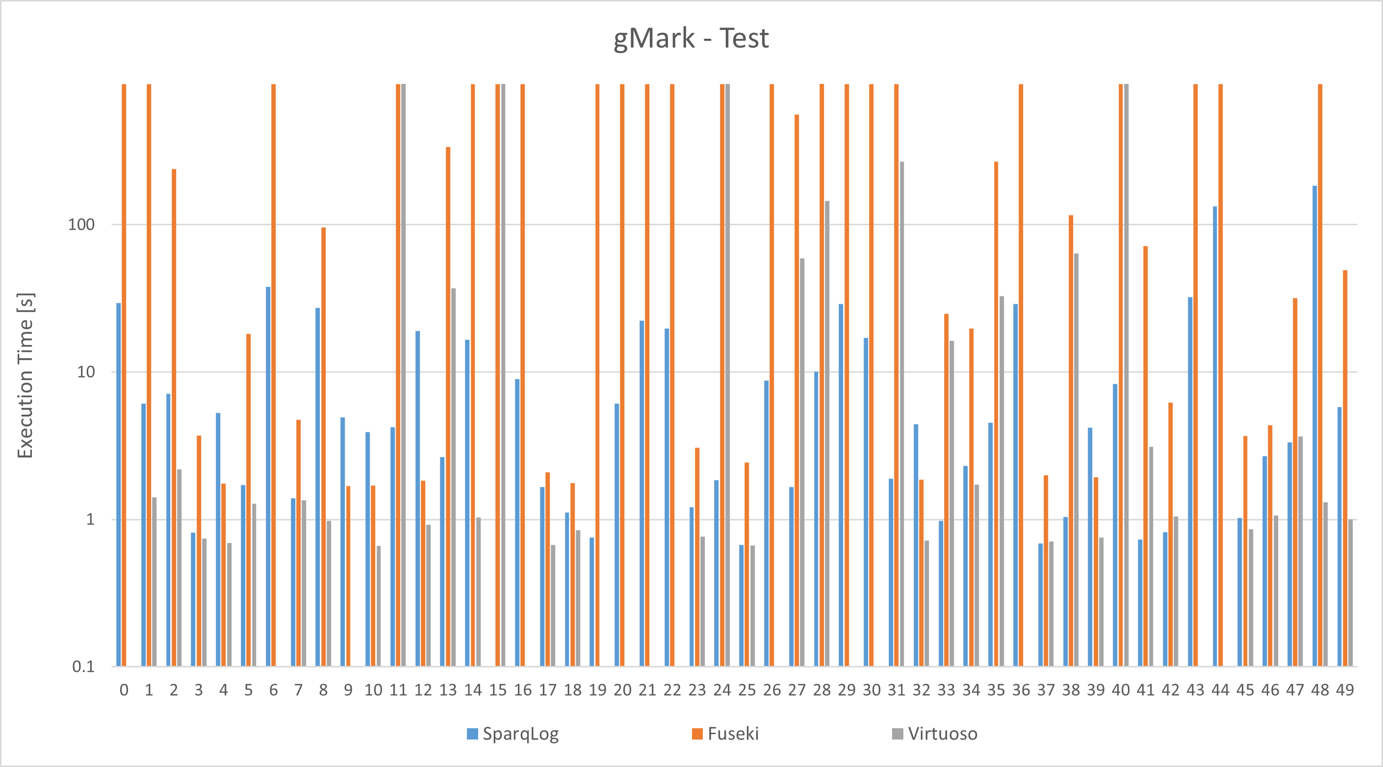
Figure 9. gMark Test Benchmark (Log Scale)

System	SparqLog	Fuseki	Virtuoso
#Not Supported	0	0	12
#Time- and Mem-Outs	1	16	1
#Incomplete Results	0	0	16
Total	1	16	29

Table 7. Benchmark Results on Social (gMark)

System	SparqLog	Fuseki	Virtuoso
#Not Supported	0	0	9
#Time- and Mem-Outs	1	21	5
#Incomplete Results	0	0	4
Total	1	21	18

Table 8. Benchmark Results on Test (gMark)

Table 7 and 8 reveal the results on the additional gMark benchmarks. Specifically, the tables state the number of queries of the respective benchmark that a system (1) does not support, (2) answered with a time- or mem-out (out-of-memory) exception, or (3) answered with an incomplete result. Furthermore, the tables present the total number of queries which could not be (correctly) answered by the systems. Figures 8 and 9 visualize the query execution time of the three systems per benchmarks. A bar reaching 900s represents a time-out. A missing bar represents a mem-out, a faulty result, or that a query was not supported. We have excluded query 31 from the gMark social benchmark and query 15 from the gMark test benchmark, as none of the three systems managed to answer these queries. In the following, we compare the results of the three systems on gMark:

Virtuoso could not (correctly) answer $48$ of the in total $100$ queries of the gMark Social and Test benchmark. Thus, it could not correctly answer almost half of the queries provided by both gMark benchmarks, which empirically reveals its dramatic limitations in answering complex property path queries. In $20$ of these $48$ cases, Virtuoso returned an incomplete result. While in solely $3$ incomplete result cases Virtuoso missed solely one tuple in the returned result multi-set, in the remaining $17$ incomplete result cases; Virtuoso produces either the result tuple null or an empty result multi-set instead of the correct non-null/non-empty result multi-set. In the other $28$ cases Virtuoso failed either due to a time-, mem-out or due to not supporting a property path with two variables. This exemplifies severe problems with handling property path queries.

Fuseki reached on $37$ of the in total $100$ queries of the gMark Social and Test benchmark a time-out (i.e., took longer than $900s$ for answering the queries). Thus, it timed-out on more than a third of gMark queries, which empirically reveals its significant limitations in answering complex property path queries.

SparqLog managed to answer $98$ of gMark’s (in total $100$) queries within less than $200s$ and timed-out on solely $2$ queries (see Figures 8 and 9). This result reveals the strong ability of our system in answering queries that contain complex property paths. Furthermore, each time when both Fuseki and SparqLog returned a result, the results were equal, even further empirically confirming the correctness of our system (i.e., that our system follows the SPARQL standard).

SP2Bench Rerun. We have rerun the SP2Bench benchmark using the same benchmark setting as for gMark. Thus, as requested by the reviewer we have rerun SP2Bench with significantly increased RAM and compared SparqLog not only to Fuseki but additionally to Virtuoso. We have visualized the result in Figure 7 and found that SparqLog reaches highly competitive performance with Virtuoso and significantly outperforms Fuseki on most queries.

In conclusion, these three benchmarks show that SparqLog (1) is highly competitive with Virtuoso on regular queries with respect to query execution time (see Figure 7, (2) even follows the SPARQL standard much more accurately than Virtuoso and supports more property path queries than Virtuoso (see Tables 7 and 8), and (3) dramatically outperforms Fuseki on query execution, while keeping its ability to follow the SPARQL standard accurately.

D.7. Complete Benchmark Results

Tables 9-11 display the complete results of the respective benchmarks. Specifically the tables contain the query id, the system’s loading time, query execution time, and total time which is the sum of the query execution and loading time. Furthermore, the column Res Equal indicates whether the result of Fuseki and Virtuoso is equal to the one from SparqLog and additionally states whether each system encountered a time-out, mem-out, or not supported exception. Note that the result of Fuseki and SparqLog is always the same when Fuseki manages to answer the query, which further exemplifies that both Fuseki and SparqLog follow the SPARQL standard precisely. However, Virtuoso violates the SPARQL standard often (indicated by many false entries in the Res Equal column of the gMark benchmarks).

	SparqLog	Fuseki				Virtuoso
Query ID	Total Time	Loading Time	Execution Time	Res Equal	Total Time	Loading Time	Execution Time	Res Equal	Total Time
0	5.390872	4.874812	20.37528	TRUE	25.25009	—	—	FALSE	Faulty Result
1	3.186824	5.046465	767.9034	TRUE	772.9499	—	—	FALSE	Faulty Result
2	19.10591	5.03212	0.026058	TRUE	5.058179	—	—	FALSE	Faulty Result
3	11.15376	4.996236	221.0903	TRUE	226.0866	—	—	FALSE	Faulty Result
4	21.87769	—	—	Time-Out	—	—	—	FALSE	Faulty Result
5	3.702722	4.737612	103.3389	TRUE	108.0765	1.502375	21.31221	TRUE	22.81458
6	6.358109	—	—	Time-Out	—	—	—	Not Supported	—
7	2.446714	4.789334	2.245069	TRUE	7.034403	1.616492	0.310986	TRUE	1.927478
8	2.087736	4.822063	0.009277	TRUE	4.83134	1.441408	0.056105	TRUE	1.497513
9	7.064603	4.63884	17.86338	TRUE	22.50222	1.496142	0.002103	TRUE	1.498245
10	4.306584	4.889473	0.021995	TRUE	4.911468	—	—	FALSE	Faulty Result
11	13.75338	4.852585	169.7659	TRUE	174.6185	—	—	FALSE	Faulty Result
12	8.887165	—	—	Time-Out	—	1.740651	0.002004	TRUE	1.742655
13	63.50253	—	—	Time-Out	—	—	—	Not Supported	—
14	2.38494	4.97689	4.229519	TRUE	9.206409	1.578675	0.019961	TRUE	1.598636
15	2.439447	4.917312	1.092629	TRUE	6.009942	1.522583	0.364891	TRUE	1.887475
16	2.190046	5.026035	1.49242	TRUE	6.518455	1.566236	0.022168	TRUE	1.588404
17	20.94913	—	—	Time-Out	—	2.796172	0.233188	TRUE	3.02936
18	2.452495	5.109881	0.011308	TRUE	5.121189	1.586266	0.006406	TRUE	1.592672
19	2.872853	5.027172	2.115648	TRUE	7.14282	—	—	FALSE	Faulty Result
20	7.979547	4.969257	0.051209	TRUE	5.020466	1.571463	0.025758	TRUE	1.59722
21	10.15052	5.041602	0.023377	TRUE	5.064978	1.675484	0.002315	TRUE	1.677799
22	50.0754	—	—	Time-Out	—	—	—	Not Supported	—
23	5.611648	—	—	Time-Out	—	3.276078	9.46E-04	TRUE	3.277024
24	4.254013	5.531002	26.98154	TRUE	32.51254	—	—	Not Supported	—
25	5.371955	4.921379	14.473	TRUE	19.39438	1.642452	87.58693	TRUE	89.22938
26	3.551616	4.961935	0.053799	TRUE	5.015734	1.802828	0.049044	TRUE	1.851872
27	58.71541	—	—	Time-Out	—	—	—	Not Supported	—
28	2.696608	5.001502	1.842646	TRUE	6.844148	—	—	FALSE	Faulty Result
29	6.087198	5.166301	444.8778	TRUE	450.0441	—	—	FALSE	Faulty Result
30	19.5853	—	—	Time-Out	—	—	—	Not Supported	—
31	Mem-Out	—	—	Time-Out	—	—	—	Time-Out	—
32	42.91233	4.727888	0.077733	TRUE	4.80562	—	—	Not Supported	—
33	157.9098	—	—	Time-Out	—	—	—	Not Supported	—
34	49.66895	—	—	Time-Out	—	—	—	Not Supported	Faulty Result
35	19.98414	4.777473	31.81758	TRUE	36.59506	—	—	FALSE	Faulty Result
36	5.953144	—	—	Time-Out	—	—	—	FALSE	#REF!
37	1.678499	5.169541	0.980466	TRUE	6.150007	1.800935	0.123026	TRUE	1.923961
38	1.635076	4.917589	0.055344	TRUE	4.972934	—	—	FALSE	Faulty Result
39	4.528049	4.856375	0.01099	TRUE	4.867365	1.785794	0.012408	TRUE	1.798202
40	6.223416	5.106296	1.540247	TRUE	6.646543	1.830541	0.002604	TRUE	1.833145
41	56.67597	—	—	Time-Out	—	—	—	Not Supported	—
42	5.210878	—	—	Time-Out	—	—	—	Not Supported	—
43	4.596554	4.697143	487.1795	TRUE	491.8766	—	—	FALSE	Faulty Result
44	8.64179	4.862944	110.3951	TRUE	115.2581	1.817118	28.31934	TRUE	30.13645
45	5.912908	—	—	Time-Out	—	—	—	Not Supported	—
46	3.006664	4.718116	0.013131	TRUE	4.731248	1.789845	0.038063	TRUE	1.827909
47	18.94113	4.876583	0.332155	TRUE	5.208737	—	—	FALSE	Faulty Result
48	2.847446	4.87816	0.286808	TRUE	5.164968	1.774782	0.042734	TRUE	1.817516
49	2.436214	4.765324	306.4633	TRUE	311.2286	—	—	FALSE	Faulty Result

Table 9. gMark Social Benchmark Results

	SparqLog	Fuseki				Virtuoso
Query ID	Total Time	Loading Time	Execution Time	Res Equal	Total Time	Loading Time	Execution Time	Res Equal	Total Time
0	29.3576	—	—	Time-Out	—	—	—	Not Supported	—
1	6.106013	—	—	Time-Out	—	1.087469	0.322955	TRUE	1.410424
2	7.146815	1.743377	237.1209	TRUE	238.8643	0.66307	1.527345	TRUE	2.190415
3	0.81259	1.745625	1.969295	TRUE	3.71492	0.674981	0.066597	TRUE	0.741577
4	5.301735	1.733303	0.018666	TRUE	1.751969	0.666493	0.026623	TRUE	0.693117
5	1.705723	1.723611	16.47228	TRUE	18.19589	0.671292	0.609226	TRUE	1.280517
6	37.87879	—	—	Time-Out	—	—	—	Not Supported	—
7	1.388953	1.739257	3.015784	TRUE	4.75504	0.674396	0.676409	TRUE	1.350805
8	27.33182	1.693349	93.86912	TRUE	95.56246	0.657102	0.319835	TRUE	0.976937
9	4.950027	1.670561	0.01266	TRUE	1.683221	—	—	FALSE	Faulty Result
10	3.90854	1.684732	0.008307	TRUE	1.693039	0.651951	0.010579	TRUE	0.662529
11	4.221005	—	—	Time-Out	—	—	—	Time-Out	—
12	19.01537	1.82695	0.011788	TRUE	1.838737	0.687586	0.229096	TRUE	0.916682
13	2.644757	1.895311	336.0234	TRUE	337.9187	0.699101	36.34624	TRUE	37.04534
14	16.52763	—	—	Time-Out	—	1.034326	8.59E-04	TRUE	1.035186
15	Mem-Out	—	—	Time-Out	—	—	—	Time-Out	—
16	8.941485	—	—	Time-Out	—	—	—	FALSE	Faulty Result
17	1.664635	1.823395	0.270428	TRUE	2.093823	0.622421	0.048782	TRUE	0.671203
18	1.118286	1.76035	0.006781	TRUE	1.767131	0.621048	0.222413	TRUE	0.843462
19	0.751237	—	—	Time-Out	—	—	—	Not Supported	—
20	6.105985	—	—	Time-Out	—	—	—	Not Supported	—
21	22.34224	—	—	Time-Out	—	—	—	Not Supported	—
22	19.75693	—	—	Time-Out	—	—	—	Not Supported	—
23	1.210083	1.840726	1.230116	TRUE	3.070842	0.643051	0.120556	TRUE	0.763607
24	1.852502	—	—	Time-Out	—	—	—	Time-Out	—
25	0.672278	1.829289	0.600554	TRUE	2.429843	0.628258	0.036516	TRUE	0.664774
26	8.776724	—	—	Time-Out	—	—	—	Not Supported	—
27	1.655394	1.686786	556.2064	TRUE	557.8932	0.678793	58.42757	TRUE	59.10637
28	10.03315	1.701909	1022.024	TRUE	1023.726	0.729646	144.8955	TRUE	145.6251
29	28.90678	—	—	Time-Out	—	—	—	Not Supported	—
30	17.07449	—	—	Time-Out	—	—	—	FALSE	Faulty Result
31	1.889749	—	—	Time-Out	—	0.767876	268.1806	TRUE	268.9484
32	4.435148	1.84552	0.011991	TRUE	1.857511	0.700008	0.018887	TRUE	0.718895
33	0.981107	1.87802	22.94484	TRUE	24.82286	0.672669	15.62866	TRUE	16.30133
34	2.307586	1.908785	17.86245	TRUE	19.77124	0.687419	1.033115	TRUE	1.720534
35	4.527377	1.812636	265.5669	TRUE	267.3796	0.687563	32.03738	TRUE	32.72494
36	29.09114	—	—	Time-Out	—	—	—	FALSE	Faulty Result
37	0.688185	1.980404	0.00798	TRUE	1.988384	0.697309	0.01165	TRUE	0.708959
38	1.04346	1.871827	113.9019	TRUE	115.7738	0.771054	63.2209	TRUE	63.99196
39	4.186533	1.914543	0.024354	TRUE	1.938897	0.717747	0.038452	TRUE	0.756199
40	8.279989	—	—	Time-Out	—	—	—	Time-Out	—
41	0.73241	1.898214	69.61925	TRUE	71.51746	0.660548	2.44178	TRUE	3.102328
42	0.817126	1.833329	4.398628	TRUE	6.231957	0.719869	0.328373	TRUE	1.048242
43	32.35511	—	—	Time-Out	—	—	—	Not Supported	—
44	133.7689	—	—	Time-Out	—	—	—	Mem-Out	—
45	1.027826	1.753663	1.929043	TRUE	3.682706	0.656611	0.199623	TRUE	0.856234
46	2.693819	1.759759	2.605928	TRUE	4.365688	0.672731	0.392371	TRUE	1.065102
47	3.325502	1.833093	29.93909	TRUE	31.77218	0.712115	2.949679	TRUE	3.661795
48	184.1826	—	—	Time-Out	—	0.892285	0.420084	TRUE	1.312369
49	5.807983	1.761885	47.55949	TRUE	49.32137	0.685809	0.314163	TRUE	0.999972

Table 10. gMark Test Benchmark Results

	SparqLog	Fuseki				Virtuoso
Query ID	Total Time	Loading Time	Execution Time	Res Equal	Total Time	Loading Time	Execution Time	Res Equal	Total Time
0	0.255653	1.370513	0.01779	TRUE	1.388303	0.924484	0.024339	TRUE	0.948822
1	0.916753	1.376974	0.531686	TRUE	1.90866	0.813104	0.141013	TRUE	0.954116
2	1.103546	1.397222	0.11726	TRUE	1.514483	0.752074	0.050747	TRUE	0.802822
3	0.957007	1.366825	0.028847	TRUE	1.395672	0.805103	0.00634	TRUE	0.811443
4	0.788907	1.358605	0.021999	TRUE	1.380604	0.773406	0.003473	TRUE	0.776879
5	2.446126	1.404242	207.2158	TRUE	208.62	0.755929	1.769996	TRUE	2.525925
6	5.827524	1.419442	43.60139	TRUE	45.02083	0.719526	0.035193	TRUE	0.754719
7	0.31812	1.455698	0.442014	TRUE	1.897712	0.656873	0.04001	TRUE	0.696883
8	3.091841	1.451437	1.853865	TRUE	3.305302	0.681998	0.132236	TRUE	0.814234
9	1.480341	1.497634	25.45474	TRUE	26.95237	0.723982	0.011736	TRUE	0.735719
10	2.385485	1.494223	0.039226	TRUE	1.533449	0.753507	0.017065	TRUE	0.770571
11	0.440275	1.494761	0.158715	TRUE	1.653476	0.773565	0.008843	TRUE	0.782408
12	0.289779	1.48597	0.019753	TRUE	1.505723	0.758892	0.007191	TRUE	0.766083
13	0.34749	1.576266	0.121115	TRUE	1.697381	0.758498	0.060892	TRUE	0.81939
14	4.737758	1.57317	0.035073	TRUE	1.608243	0.748497	0.002614	TRUE	0.751111
15	1.835838	1.552763	0.01046	TRUE	1.563222	0.737808	0.012529	TRUE	0.750336
16	0.212753	1.547268	0.009173	TRUE	1.556441	0.734842	7.08E-04	TRUE	0.73555

Table 11. SP2Bench Benchmark Results

D.8. Ontological Reasoning Results

One of the main advantages of our SparqLog system is that it provides a uniform and consistent framework for reasoning and querying Knowledge Graphs. We therefore wanted to measure the performance of query answering in the presence of an ontology. Since Fuseki and Virtuoso do not provide such support, we now compare SparqLog with Stardog, which is a commonly accepted state-of-the-art system for reasoning and querying within the Semantic Web. Furthermore, we have also created a benchmark based on SP2Bench’s dataset that provides property path queries and ontological concepts such as subPropertyOf and subClassOf. We have provided this benchmark in the supplementary material.

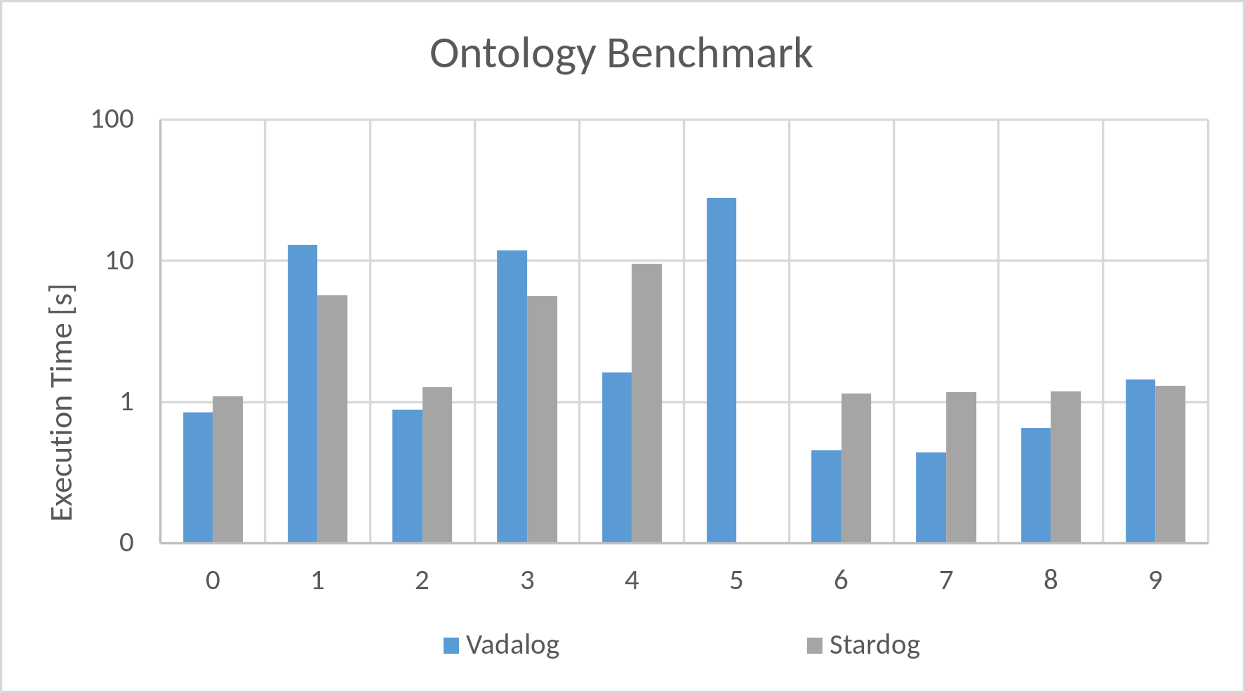
Figure 10. Ontology Benchmark

Figure 10 shows the outcome of these experiments. In summary, we note that SparqLog is faster than Stardog on most queries. Particularly interesting are queries 4 and 5, which contain recursive property path queries with two variables. Our engine needs on query 4 only about a fifth of the execution time of Stardog and it can even answer query 5, on which Stardog times outs (using a timeout of $900s$). On the other queries, Stardog and SparqLog perform similarly.

Appendix E More on Datalog^±

Recall from Section 3.1 that query answering under an ontology defined by Datalog^± program comes down to solving an entailment problem. More precisely, let $Q(\vec{z})$ be a CQ with free variables $\vec{z}$ over database $D$ and let an ontology be expressed by Datalog^± program $\Pi$. Then the answers to $Q(\vec{z})$ over $D$ under ontology $\Pi$ are defined as $\{\vec{a}\mid\Pi\cup D\models Q(\vec{a})\}$, where $\vec{a}$ is a tuple of the same arity as $\vec{z}$ with values from the domain of $D$.

Canonical model and the chase

Note that $\Pi\cup D$ can have many models. A canonical model is obtained via the chase, which is defined as follows: We say that a rule $\rho\in\Pi$ with head $p(\vec{z})$ is applicable to an instance $I$ if there exists a homomorphism $h$ from the body of $\rho$ to $I$. We may then carry out a chase step, which consists in adding atom $h^{\prime}(p(\vec{z}))$ to instance $I$, where $h^{\prime}$ coincides with $h$ on all variables occurring in the body of $\rho$ and $h^{\prime}$ maps each existential variable in $p(\vec{z})$ to a fresh labelled null not occurring in $I$. A chase sequence for database $D$ and program $\Pi$ is a sequence of instances $I_{0},I_{1},\dots$ obtained by applying a sequence of chase steps, starting with $I_{0}=D$. The union of instances obtained by all possible chase sequences is referred to as $\mathit{Chase}(D,\Pi)$. The labelled nulls in $\mathit{Chase}(D,\Pi)$ play the same role as blank nodes in an RDF graph, i.e., resources for which the concrete value is not known. The importance of $\mathit{Chase}(D,\Pi)$ comes from the equivalence $\Pi\cup D\models Q(\vec{a})\Leftrightarrow\mathit{Chase}(D,\Pi)\models Q(\vec{a})$ (Fagin et al., 2005). Note however that, in general, $\mathit{Chase}(D,\Pi)$ is infinite. Hence, the previous equivalence does not yield an algorithm to evaluate a CQ $Q(\vec{z})$ w.r.t. database $D$ and program $\Pi$. In fact, without restriction, this is an undecidable problem (Johnson and Klug, 1984). Several subclasses of Datalog^± have thus been presented (Fagin et al., 2005; Calì et al., 2013, 2010, 2010; Baget et al., 2009; Baget et al., 2011; Arenas et al., 2018) that ensure decidability of CQ answering (see (Calì et al., 2013) for an overview).

Bag semantics of Datalog

In (Mumick et al., 1990), a bag semantics of Datalog was introduced based on derivation trees. Given a database $D$ and Datalog program $\Pi$, a derivation tree (DT) is a tree $T$ with node and edge labels, such that either (1) $T$ consists of a single node labelled by an atom from $D$ or (2) $\Pi$ contains a rule $\rho\colon\ H\leftarrow A_{1},A_{2},\ldots,A_{k}$ with $k>0$, and there exist DTs $T_{1},\ldots,T_{k}$ whose root nodes are labelled with atoms $C_{1},\ldots,C_{k}$ such that $A_{1},\ldots,A_{k}$ are simultaneously matched to $C_{1},\ldots,C_{k}$ by applying some substitution $\theta$, and $T$ is obtained as follows: $T$ has a new root node $r$ with label $H\theta$ and the $k$ root nodes of the DTs $T_{1},\ldots,T_{k}$ are appended as child nodes of $r$ in this order. All edges from $r$ to its child nodes are labelled with $\rho$. Then the bag semantics of program $\Pi$ over database $D$ consists of all ground atoms derivable from $D$ by $\Pi$, and the multiplicity $m\in\mathbb{N}\cup\{\infty\}$ of each such atom $A$ is the number of possible DTs with root label $A$. Datalog with bag semantics is readily extended by stratified negation (Mumick and Shmueli, 1993): the second condition of the definition of DTs now has to take negative body atoms in a rule $\rho\colon H\leftarrow A_{1},A_{2},\ldots,A_{k},\neg B_{1},\dots\neg B_{\ell}$ with $k>0$ and $\ell\geq 0$ with head atom $H$ from some stratum $i$ into account in that we request that none of the atoms $B_{1}\theta,\dots B_{\ell}\theta$ can be derived from $D$ via the rules in $\Pi$ from strata less than $i$.

Bag semantics via set semantics of Warded Datalog^±

In (Bertossi et al., 2019) it was shown how Datalog with bag semantics can be transformed into Warded Datalog^± with set semantics. The idea is to replace every predicate $P(\ldots)$ by a new version $P(.\ ;\ldots)$ with an extra, first argument to accommodate a labelled null which is interpreted as tuple ID (TID). Each rule in $\Pi$ of the form

$\rho\colon H(\bar{x})\ \leftarrow\ A_{1}(\bar{x}_{1}),A_{2}(\bar{x}_{2}),\ldots,A_{k}(\bar{x}_{k})$, with $k>0,\bar{x}\subseteq\cup_{i}\bar{x}_{i}$

is then transformed into the Datalog^± rule

$\rho^{\prime}\colon\ \exists z\ H(z;\bar{x})\leftarrow A_{1}(z_{1};\bar{x}_{1}),A_{2}(z_{2};\bar{x}_{2}),\ldots,A_{k}(z_{k};\bar{x}_{k})$,

with fresh, distinct variables $z,z_{1},\ldots,z_{k}$. Some care (introducing auxiliary predicates) is required for rules with negated body atoms so as not to produce unsafe negation. A Datalog rule
$\rho\colon H(\bar{x})\ \leftarrow\ A_{1}(\bar{x}_{1}),\ldots,A_{k}(\bar{x}_{k}),\neg B_{1}(\bar{x}_{k+1}),\ldots,\neg B_{\ell}(\bar{x}_{k+\ell})$ with, $\bar{x}_{k+1},\ldots,\bar{x}_{k+\ell}\subseteq\bigcup_{i=1}^{k}\bar{x}_{i}$ is replaced by $\ell+1$ rules in the corresponding Datalog^± program $\Pi^{\prime}$:

$\rho^{\prime}_{0}\colon\exists zH(z;\bar{x})\leftarrow A_{1}(z_{1};\bar{x}_{1}),\ldots,A_{k}(z_{k};\bar{x}_{k})$,
$\rho^{\prime}_{0}\colon\exists zH(z;\bar{x})\leftarrow$ $\neg\mathit{Aux}_{1}^{\rho}(\bar{x}_{k+1}),\ldots,\neg\mathit{Aux}_{\ell}^{\rho}(\bar{x}_{k+\ell})$,
$\rho^{\prime}_{i}\colon\mathit{Aux}_{i}^{\rho}(\bar{x}_{k+i})\leftarrow B_{i}(z_{i};\bar{x}_{k+i}),\ \ i=1,\ldots,\ell$.

The resulting Datalog^± program $\Pi^{\prime}$ is trivially warded since the rules thus produced contain no dangerous variables at all. Moreover, it is proved in (Bertossi et al., 2019) that an atom $P(\vec{a})$ is in the DT-defined bag semantics of Datalog program $\Pi$ over database $D$ with multiplicity $m\in\mathbb{N}\cup\{\infty\}$, iff $\mathit{Chase}(D,\Pi^{\prime})$ contains atoms of the form $P(t;\vec{a})$ for $m$ distinct labelled nulls $t$ (i.e., the tuple IDs).