A qubit regularization of asymptotic freedom at the BKT transition without fine-tuning

Abstract

We propose a two-dimensional hard core loop-gas model as a way to regularize the asymptotically free massive continuum quantum field theory that emerges at the BKT transition. Without fine-tuning, our model can reproduce the universal step-scaling function of the classical lattice XY model in the massive phase as we approach the phase transition. This is achieved by lowering the fugacity of Fock-vacuum sites in the loop-gas configuration space to zero in the thermodynamic limit. Some of the universal quantities at the BKT transition show smaller finite size effects in our model as compared to the traditional XY model. Our model is a prime example of qubit regularization of an asymptotically free massive quantum field theory in Euclidean space-time and helps understand how asymptotic freedom can arise as a relevant perturbation at a decoupled fixed point without fine-tuning.

The success of the Standard Model of particle physics shows that at a fundamental level, nature is well described by a continuum Quantum Field Theory (qft). Understanding qfts non-perturbatively continues to be an exciting area of research, since defining them in a mathematically unambiguous way can be challenging. Most definitions require some form of short-distance (ultraviolet (uv)) regularization, which ultimately needs to be removed. Wilson has argued that continuum qfts arise near fixed points of renormalization group flows [1]. This has led to the concept of universality, which says that different regularization schemes can lead to the same qft. Following Wilson, traditional continuum quantum field theories are usually regulated non-perturbatively on a space-time lattice by replacing the continuum quantum fields by lattice quantum fields and constructing a lattice Hamiltonian with a quantum critical point where the long distance lattice physics can be argued to be the desired continuum qft. However, universality suggests that there is a lot of freedom in choosing the microscopic lattice model to study a particular qft of interest.

Motivated by this freedom and to study continuum quantum field theories in real time using a quantum computer, the idea of qubit regularization has gained popularity recently [2, 3, 4, 5, 6, 7, 8, 9, 10]. Unlike traditional lattice regularization, qubit regularization explores lattice models with a strictly finite local Hilbert space to reproduce the continuum qft of interest. Euclidean qubit regularization can be viewed as constructing a Euclidean lattice field theory with a discrete and finite local configuration space, that reproduces the continuum Euclidean qft of interest at a critical point. If the target continuum theory is relativistic, it would be natural to explore Euclidean qubit regularized models that are also symmetric under space-time rotations. However, this is not necessary, since such symmetries can emerge at the appropriate critical point. Lattice models with a finite dimensional Hilbert space that can reproduce continuum qfts of interest were introduced several years ago through the D-theory formalism [11, 12] and has been proposed for quantum simulations [13, 14]. In contrast to qubit regularization, the D-theory approach allows the local Hilbert space to grow through an additional dimension when necessary. In this sense, qubit regularization can be viewed as the D-theory approach for those qfts where a strictly finite Hilbert space is sufficient to reproduce the desired QFT.

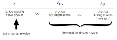
Figure 1: Length scales in a lattice field theory that reproduces asymptotically free quantum field theories.

Examples of using qubit regularization to reproduce continuum qfts in the infrared (ir) are well known. Quantum spin models with a finite local Hilbert space are known to reproduce the physics of classical spin models with an infinite local Hilbert space near Wilson-Fisher fixed points [15]. They can also reproduce qfts with topological terms like the Wess-Zumino-Witten theories [16]. Gauge fields have been proposed to emerge dynamically at some quantum critical points of simple quantum spin systems [17]. From the perspective of Euclidean qubit regularization, recently it was shown that Wilson-Fisher fixed points with $O(N)$ symmetries can be recovered using simple qubit regularized space-time loop models with $N+1$ degrees of freedom per lattice site [18, 19]. Similar loop models have also been shown to produce other interesting critical behavior [20, 21, 22]. Loop models are extensions of dimer models, which are also known to describe interesting critical phenomena in the ir [23, 24]. All this evidence shows that Euclidean qubit regularization is a natural way to recover continuum qfts that emerge via ir fixed points of lattice models.

A non-trivial question is whether we can also recover the physics of ultraviolet fixed points (UV-FPs), using qubit regularization. In particular, can we recover massive continuum qfts which are free in the UV but contain a marginally relevant coupling? Examples of such asymptotically free (af) theories include two-dimensional spin models and four dimensional non-Abelian gauge theories. In the D-theory approach, there is strong evidence that the physics at the uv scale can indeed be recovered exponentially quickly as one increases the extent of the additional dimension [25, 26, 27, 28, 29]. Can the Gaussian nature of the uv theory emerge from just a few discrete and finite local lattice degrees of freedom, while the same theory then goes on to reproduce the massive physics in the ir? For this we will need a special type of quantum criticality where three length scales, as sketched in Fig. 1, emerge. There is a short lattice length scale $a$, where the non-universal physics depends on the details of the qubit regularization, followed by an intermediate length scale ${\ell_{\rm UV}}\gg a$, where the continuum uv physics sets in and the required Gaussian theory emerges. Finally, at long length scales ${\ell_{\rm IR}}\gg{\ell_{\rm UV}}$, the non-perturbative massive continuum quantum field theory emerges due to the presence of a marginally relevant coupling in the uv theory. The qubit regularized theory thus reproduces the universal continuum qft in the whole region $\ell_{\rm UV}$ to $\ell_{\rm IR}$. The special quantum critical point must be such that $\ell_{\rm UV}/a\rightarrow\infty$.

Recently, a quantum critical point with these features was discovered in an attempt to find a qubit regularization of the asymptotically free massive non-linear O(3) sigma model in two space-time dimensions in the Hamiltonian formulation [30]. Using finite size scaling techniques, it was shown that the qubit regularized model recovers all the three scales. In this paper, we report the discovery of yet another example of a quantum critical point with similar features. In the current case, it is a Euclidean qubit regularization of the asymptotically free massive continuum quantum field theory that arises as one approaches the Berezenski-Kosterlitz-Thouless (bkt) transition from the massive phase [31, 32]. In both these examples, the qubit regularized model is constructed using two decoupled theories and the af-qft emerges as a relevant perturbation at a decoupled quantum critical point. The coupling between the theories plays the role of the perturbation that creates the three scales, as illustrated in the RG flow shown in Fig. 2. An interesting feature of this discovery is that there is no need for fine-tuning to observe some of the universal features of the bkt transition that have been unattainable in practice with other traditional regularizations [33].

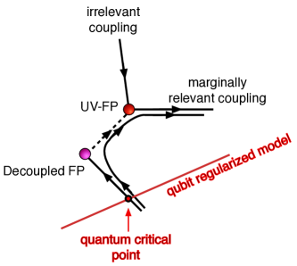
Figure 2: An illustration of the RG flow of the qubit regularized model that reproduces the physics of the asymptotically free qfts in this paper and in [30]. At the decoupled quantum critical point, both qubit models describe the physics of a critical system containing two decoupled theories. However, when a small non-zero coupling is introduced between the theories, the long distance physics flows towards the desired universal physics of the uv-fixed point theory.

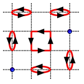
Figure 3: The left figure shows an illustration of a self-avoiding oriented loop configuration. There are also Fock-vacuum sites, shown as blue circles, which have a weight $\lambda$. The oriented loop configuration can also be viewed as a close packed dimer configurations on two layers, as illustrated on the right. The interlayer dimers would map to the Fock-vacuum sites, while the intralayer oriented dimers would form closed oriented loops, all which have weight one. The dimers are oriented from even sites to odd sites on one layer and in the opposite direction on the other layer. This mapping to the dimer model shows that the loop model is critical when $\lambda=0$.

The bkt transition is one of the most widely studied classical phase transitions, since it plays an important role in understanding the finite temperature superfluid phase transition of two-dimensional systems [34]. One simple lattice model that captures the universal behavior of the physics close to the phase transition is the classical two-dimensional XY model on a square lattice given by the classical action,

$$S=-\beta\sum_{\langle ij\rangle}\cos(\theta_{i}-\theta_{j}),$$ (1)

where the lattice field $0\leq\theta_{i}<2\pi$ is an angle associated to every space-time lattice site $i$ and $\langle ij\rangle$ refers to the nearest neighbor bonds with sites $i$ and $j$. The lattice field naturally lives in an infinite dimensional Hilbert space of the corresponding one dimensional quantum model. Using high precision Monte Carlo calculations, the bkt transition has been determined to occur at the fine-tuned coupling of $\beta_{c}\approx 1.1199(1)$ [35, 36]. The Villain model is another lattice model which is friendlier for analytic calculations and has been used to uncover the role of topological defects in driving the phase transition [37]. More recently, topological lattice actions which seem to suppress vortices and anti-vortices but still drive the bkt transition have also been explored [38].

As one approaches the bkt transition from the massive phase, the long distance physics of the Eq. 1 is known to be captured by the sine-Gordon model whose Euclidean action is given by[39],

$$S=\int dxdt\ \left[\frac{1}{2t}(\partial_{\mu}\theta_{1})^{2}+\frac{t}{8\pi^{2}}(\partial_{\mu}\theta_{2})^{2}-\frac{At}{4\pi^{2}}\cos\theta_{2}\right]$$ (2)

where $t\geq\pi/2$. The field $\theta_{1}(x,t)$ captures the spin-wave physics while the vortex dynamics is captured by the field $\theta_{2}(x,t)$. The BKT transition in this field theory language occurs at $t=\pi/2$ where the $\cos\theta_{2}$ term becomes marginal as one approaches the critical point and the physics is governed by a free Gaussian theory. In this sense, the long distance physics of the lattice XY model, as $\beta$ is tuned to $\beta_{c}$ from smaller values, is an asymptotically free massive Euclidean continuum qft.

Qubit regularizations of the classical XY-model have been explored recently using various quantum spin formulations [40]. Lattice models based on the spin-1 Hilbert space are known to contain rich phase diagrams [41], and quantum field theories that arise at some of the critical points can be different from those that arise at the bkt transition. Also, the presence of a marginally relevant operator at the BKT transition can make the analysis difficult, especially if the location of the critical point is not known. In these cases, it becomes a fitting parameter in the analysis, increasing the difficulty. Since in our model the location of the critical point is known, our model can be analyzed more easily.

The model we consider in this work is a variant of the qubit regularized XY model introduced in Euclidean space recently [4]. The model can be viewed as a certain limiting case of the classical lattice XY-model Eq. 1 written in the world-line representation [42], where the bosons are assumed to be hard-core. The partition function of our model is a sum of weights associated with configurations of oriented self-avoiding loops on a square lattice with Fock-vacuum sites. An illustration of the loop configuration is shown as the left figure in Fig. 3. The main difference between our model in this work and the one introduced previously is that closed loops on a single bond are now allowed. Such loops seemed unnatural in the Hamiltonian framework that motivated the previous study, but seem to have profoundly different features in two dimensions [43]. It is also possible to view the loop configurations of our model as a configuration of closed packed oriented dimers on two layers of square lattices. The dimer configuration corresponding to the loop configuration is shown on the right in Fig. 3. The dimer picture of the partition function arises as a limiting case of a model involving two flavors of staggered fermions, introduced to study the physics of symmetric mass generation [44, 45, 46]. In this view point the inter-layer dimers (or Fock vacuum sites) resemble t’Hooft vertices (or instantons) in the fermionic theory. Using this connection, the partition function of our model can be compactly written as the Grassmann integral

$$Z\ =\int\ [d{\bar{\psi}}d{\psi}]\ [d{\bar{\chi}}d{\chi}]\ \exp\Big{(}\lambda\ \sum_{i}\ {\bar{\psi}}_{i}{\psi}_{i}{\bar{\chi}}_{i}{\chi}_{i}\Big{)}$$

$$\times\ \exp\Big{(}\sum_{\langle ij\rangle}\big{(}{\bar{\psi}}_{i}{\psi}_{i}{\bar{\psi}}_{j}{\psi}_{j}+{\bar{\chi}}_{i}{\chi}_{i}{\bar{\chi}}_{j}{\chi}_{j}\big{)}\Big{)}$$ (3)

where on each site $i$ of the square lattice we define four Grassmann variables ${\bar{\psi}}_{i}$, ${\psi}_{i}$, ${\bar{\chi}}_{i}$ and ${\chi}_{i}$. We consider periodic lattices with $L$ sites in each direction. Using the fermion bag approach [47], we can integrate the Grassmann variables and write the partition function as a sum over dimer configurations whose weight is given by $\lambda^{N_{I}}$ where $N_{I}$ is the number of instantons (or Fock-vacuum sites). Thus, $\lambda$ plays the role of the fugacity of Fock-vacuum sites. It is easy to verify that the action of our model is invariant under ${\bar{\psi}}_{j}{\psi}_{j}\rightarrow e^{i\sigma_{j}\theta}{\bar{\psi}}_{j}{\psi}_{j}$ and ${\bar{\chi}}_{j}{\chi}_{j}\rightarrow e^{-i\sigma_{j}\theta}{\bar{\chi}}_{j}{\chi}_{j}$ where $\sigma_{j}=\pm$ tracks the parity of the site $j$. This U(1) symmetry is connected to the bkt transition and in order to track it, the dimers are given an orientation as explained in Fig. 3.

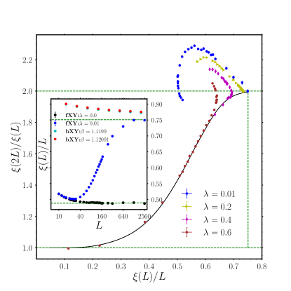
Figure 4: The figure shows the universal ssf (i.e., $\xi(2L)/\xi(L)$ vs. $\xi(L)/L$) obtained from the XY-model Eq. 1 (solid line) [48] and compares it with data from the model Eq. 3 at $\lambda=0.6$,$0.4$,$0.2$,and $0.01$ for various lattice sites. For small values of $L$, our data deviates from the solid line since $L<{\ell_{\rm UV}}$, but for $L\gtrsim{\ell_{\rm UV}}$, the data begin to fall on the line and then follows it for larger values of $L$. Since $\lambda=0.01$ is close to the critical point, the data approaches the universal UV prediction (see [35]) of $\xi(L)/L=0.7506912...$. To show this more clearly, we plot $\xi(L)/L$ as a function of $L$ for $\lambda=0$ and $\lambda=0.01$ in the inset. Note that the large $L$ behavior of $\lambda=0$ is very different from that of $\lambda=0.01$. While the former stabilizes at $\xi(L)/L=0.4889(6)$, the latter approaches $\xi(L)/L=0.7506912...$ as expected, when $L\sim{\ell_{\rm UV}}$. For comparison, in the inset we also show the data from the traditional $XY$ model (Eq. 1) which is still far from the universal value due to logarithmic corrections as explained in [35]. Since $\lambda=0.01$ is not the critical point, we predict that $\xi(L)/L$ will eventually turn around for $L\gg{\ell_{\rm UV}}$ and approach zero.

Using worm algorithms (see [49]) we study our model for various values of $L$ and $\lambda$. At $\lambda=0$, one gets two decoupled layers of closed packed dimer models, which is known to be critical [50, 51, 52, 53]. The effect of $\lambda\neq 0$ was studied several years ago, and it was recognized that there is a massive phase for sufficiently large values of $\lambda$ [54, 55]. However, the scaling of quantities as $\lambda\rightarrow 0$ was not carefully explored. Recently, the subject was reconsidered, and a crossover phenomenon was observed for small $\lambda$ as a function of $L$. An understanding of this crossover was largely left unresolved as a puzzle [56]. In this paper, we demonstrate that the observed crossover phenomena captures the asymptotic freedom of Eq. 2. We do this by comparing the universal behavior of Eq. 3 with the traditional XY model Eq. 1 near the massive phase of the bkt transition [35, 57, 58].

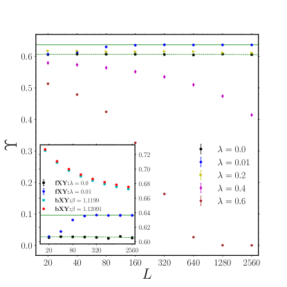
Figure 5: The figure shows the helicity modulus $\Upsilon$ as a function of $L$ for $\lambda=0.6$, $0.4$, $0.2$,$0.01$ and $0.0$. We expect $\Upsilon\rightarrow 0$ for $L\gg{\ell_{\rm UV}}$ when $\lambda\neq 0$. This is clearly seen at $\lambda=0.6$. At $\lambda=0.4$, since ${\ell_{\rm UV}}$ is larger, we only see the initial part of the decrease towards zero. At $\lambda=0.2$, ${\ell_{\rm UV}}$ is even larger, and so we only observe the flat part expected in the uv. At the uv fixed point we expect $\Upsilon\approx 2/\pi$. When $\lambda=0.01$ we do observe the data converging well to this universal value (top solid line). Since $\lambda=0.01$ is not really the critical point, this line too will eventually turn around at very large values of $L$ and go to zero. On the other hand when $\lambda=0$ we find that $\Upsilon\approx 0.606$ in the large $L$ limit [48]. We demonstrate the difference between $\lambda=0$ and $\lambda=0.01$ in the inset, where we also show the values of the helicity modulus in the traditional XY model Eq. 1 at $\beta\approx\beta_{c}=1.1199(1)$. Note that the values from the traditional model are far from $2/\pi$, a well-known difficulty due to large logarithmic corrections. In contrast, our qubit model is able to recover the uv physics more easily.

To compare universal behaviors of Eq. 1 and Eq. 3 we compute the second moment finite size correlation length $\xi(L)$ defined as $\xi(L)\ =\ \sqrt{(\chi/F)-1}/(2\sin(\pi/L))$ (see [59]), where $\chi=G(0)$ and $F=G(2\pi/L)$ are defined through the two point correlation function

$$G(p)=\sum_{j}e^{ipx}\langle{\cal O}^{+}_{(x,t)}{\cal O}^{-}_{(0,0)}\rangle.$$ (4)

In the above relation $j$ is the space-time lattice site with coordinates $(x,t)$ and ${\cal O}^{+}_{j},{\cal O}^{-}_{j}$ are appropriate lattice fields in the two models. In the $XY$ model ${\cal O}^{+}_{j}=e^{i\theta_{j}},{\cal O}^{-}_{j}=e^{-i\theta_{j}}$, while in the dimer model ${\cal O}^{+}_{j}={\cal O}^{-}_{j}={\bar{\psi}}_{j}{\psi}_{j}$. We demonstrate that the step-scaling function (SSF) (i.e., the dependence of $\xi(2L)/\xi(L)$ on $\xi(L)/L$) of the two lattice models show excellent agreement with each other in the scaling regime $\ell_{UV}\gg a$, in Fig. 4.

Another interesting universal result at the bkt transition is the value of the helicity modulus, which can be defined using the relation, $\Upsilon\ =\ \langle Q_{w}^{2}\rangle$ where $Q_{w}$ is the spatial winding number of bosonic worldlines. In the XY model Eq. 1, it is usually defined using a susceptibility of a twist parameter in the boundary conditions [35]. In our model, we can easily compute the winding charge $Q_{w}$ in each loop configuration illustrated in Fig. 3. The universal result in the massive phase as we approach the BKT transition is that $\Upsilon\approx 2/\pi$ in the uv up to exponentially small corrections [35], although in the ir $\Upsilon=0$. While it is difficult to obtain the uv value in lattice calculations using the traditional model Eq. 1, in our model, we can see it emerge nicely at $\lambda=0.01$. We demonstrate this in Fig. 5. Again, as expected, the value of $\Upsilon$ when $\lambda=0$ is very different, since it is a theory of free bosons but at a different coupling. Using the different value of the coupling gives $\Upsilon\ \approx 0.606$ [48]. Our results provide strong evidence that the af-qft at the BKT transition emerges from our dimer model when we take the limit $L\rightarrow\infty$ followed by $\lambda\rightarrow 0$. The opposite limit leads to the critical theory of the decoupled dimer model.

Acknowledgments: We are grateful to J. Pinto Barros, S. Bhattacharjee, T. Bhattacharya, H. Liu, A. Sen, H. Singh and U.-J. Wiese for inspiring discussions. We acknowledge use of the computing clusters at SINP, and the access to Piz Daint at the Swiss National Supercomputing Centre, Switzerland under the ETHZ’s share with the project IDs go24 and eth8. Support from the Google Research Scholar Award in Quantum Computing and the Quantum Center at ETH Zurich is gratefully acknowledged. S.C’s contribution to this work is based on work supported by the U.S. Department of Energy, Office of Science — High Energy Physics Contract KA2401032 (Triad National Security, LLC Contract Grant No. 89233218CNA000001) to Los Alamos National Laboratory. S.C is supported by a Duke subcontract based on this grant. S.C’s work is also supported in part by the U.S. Department of Energy, Office of Science, Nuclear Physics program under Award No. DE-FG02-05ER41368.

Supplementary Material

Appendix A Universal values of $\Upsilon$ for $\lambda=0$ and $\lambda\neq 0$

In this section we explain the two different values of the helicity modulus $\Upsilon$ for our model when $\lambda=0$ and $\lambda\rightarrow 0$. When $\lambda=0$ our model maps into two identical but decoupled layers of closed packed classical dimer models. As has already been explained in the literature (see for example  [23, 53]), each layer can be mapped to the theory of a free compact scalar field with the action

$$S=\frac{1}{2t}\int d^{2}x(\partial_{\mu}\theta(x))^{2}.$$ (5)

with $t=4\pi$. One can compute $\Upsilon$ starting with Eq. 5, by noting that the scalar fields have winding number configurations labeled by $n_{x}$:

$$\theta(x)\ =\ \frac{2\pi xn_{x}}{L_{x}}+\varphi(x),$$ (6)

where $\varphi(x)$ is a smooth fluctuation that is independent of winding number $n_{x}$. The value of the action in each winding sector in a finite space-time volume is then given by

$$S(n_{x})=\frac{2\pi^{2}n_{x}^{2}}{t}\frac{L_{y}}{L_{x}}+S_{0},$$ (7)

where $S_{0}$ is the action from the usual fluctuations in the zero winding number sector. Using $L_{x}=L_{y}$, we can compute $\Upsilon$ using its connection to the average of the square of the winding numbers,

$$\Upsilon\ =\ \braket{(Q_{x})^{2}}=\frac{\sum_{n_{x}}n_{x}^{2}\cdot{\rm e}^{-\frac{2\pi^{2}n_{x}^{2}}{t}}}{\sum_{n_{x}}{\rm e}^{-\frac{2\pi^{2}n_{x}^{2}}{t}}}$$ (8)

Numerically evaluating this expression for $t=4\pi$ we obtain $\Upsilon\ =0.303426...$ for a each layer of our dimer model. Our value of $0.606852...$ is due to the presence of two decoupled layers.

In contrast, in the limit $\lambda\rightarrow 0$, we need to consider the physics at the BKT transition and so we begin with the action

$$S=\int d^{2}x\ \left[\frac{1}{2\tilde{t}}(\partial_{\mu}\theta_{1})^{2}+\frac{\tilde{t}}{8\pi^{2}}(\partial_{\mu}\theta_{2})^{2}-\frac{A\tilde{t}}{4\pi^{2}}\cos\theta_{2}\right]$$ (9)

and focus at $\tilde{t}=\pi/2$. At this coupling the last term is irrelevant and $\Upsilon$ gets dominant contribution from the $\theta_{2}$ field. In this we can still use Eq. 8 but need to substitute $t=4\pi^{2}/\tilde{t}=8\pi$. Substituting we get $\Upsilon=0.636508...$ which is approximately $2/\pi$.

Appendix B Worm Algorithm

In this section, we discuss the worm algorithm we use to simulate the model with the partition function,

$$Z\ =\int\ [d{\bar{\psi}}d{\psi}]\ [d{\bar{\chi}}d{\chi}]\ \exp\Big{(}\lambda\ \sum_{i}\ {\bar{\psi}}_{i}{\psi}_{i}{\bar{\chi}}_{i}{\chi}_{i}\Big{)}$$

$$\times\ \exp\Big{(}\sum_{\langle ij\rangle}\big{(}{\bar{\psi}}_{i}{\psi}_{i}{\bar{\psi}}_{j}{\psi}_{j}+{\bar{\chi}}_{i}{\chi}_{i}{\bar{\chi}}_{j}{\chi}_{j}\big{)}\Big{)}$$ (10)

as introduced in the main paper. These algorithms are well known [49], and can be divided into three parts: Begin, Move, and End.

1. Begin: pick a site at random and denote it as tail, and there are the following two possibilities: (A) either it has a bond connected to it on the other layer (which we call an instanton, or an interlayer dimer), or, (B) it has a bond connected to it on the same layer (which we call a dimer).

   • For the case (A), propose to remove the instanton, and put the worm head on the same site at the different layer, with a probability $1/\lambda$. If accepted, then begin the worm update, otherwise go to (1).

   • For the case (B), pick the other site to which the dimer is connected as the head, and begin the worm update.

2. Move: Propose to move the worm head to one of the $(2D+1)$ neighbor sites of head with an equal probability, which can either be on the same layer ($2D$ choices), or on the different layer (one choice). Denote the proposed new site as site0, and the following possibilities can occur, provided that site0 is not the tail:

   • site0 is on the same layer, and has an instanton connected to it. Propose to remove the instanton with a probability $1/\lambda$. If accepted, place the head at site0, but on the different layer.

   • site0 is on the same layer, and has a dimer connected to it (joining site0 and $y$). Move the head to the site $y$ with a probability 1, and simultaneously insert a dimer between head and site0.

   • site0 is on the different layer, then propose if an instanton can be created. If yes, then move the position of the head to $y$ in the other layer, where $y$ is the other end of the dimer connecting site0 and $y$.

3. End: If at any stage in the algorithm, the site0 is the tail, then propose to end the worm update. If the site0 $=$ tail is on the same layer, then end the update by putting a dimer between the head and tail with a probability 1. If, on the other hand, they are on different layers, the worm update ends with a probability $\lambda$, leading to the addition of an extra instanton.

Appendix C Exact vs Monte Carlo results on a $2\times 2$ lattice

In this work, we compute two independent fermion bilinear susceptibilities defined as

$$\chi_{1}=\frac{1}{2V}\sum\limits_{\begin{subarray}{c}i,j\\ i\neq j\end{subarray}}\left\langle\bar{\psi}_{i}\psi_{i}\bar{\psi}_{j}\psi_{j}\right\rangle,$$ (11)

$$\chi_{2}=\frac{1}{2V}\sum\limits_{\begin{subarray}{c}i,j\\ i\neq j\end{subarray}}\left\langle\bar{\psi}_{i}\psi_{i}\bar{\chi}_{j}\chi_{j}\right\rangle,$$ (12)

where $\chi_{1}$ is an observable that can be defined even on a single layer, while $\chi_{2}$ is involves both the layers. When the coupling $\lambda=0$, the two layers are completely decoupled from each other and we get $\chi_{2}=0$. Another quantity we compute is the average density of Fock vacuum sites or inter-layer dimers (which we also view as instantons), defined as

$$\rho=\frac{1}{V}\sum\limits_{i}\left\langle\bar{\psi}_{i}\psi_{i}\bar{\chi}_{i}\chi_{i}\right\rangle,$$ (13)

where the expectation value is defined as

$$\left\langle{\cal O}\right\rangle=\frac{1}{Z}\int[\mathcal{D}\bar{\psi}\mathcal{D}\psi]\hskip 2.84544pt[\mathcal{D}\bar{\chi}\mathcal{D}\chi]\hskip 2.84544pt{\cal O}\hskip 2.84544pte^{-S[\bar{\psi},\psi,\bar{\chi},\chi]}.$$ (14)

Since every site is populated by either a Fock-vacuum site or an intra-layer dimer, the average intra-layer dimer density is not an independent observable. We can always compute it from the Fock vacuum sites (instanton) density $\rho$.

In order to test out algorithm, we focus on exact results on a $2\times 2$ lattice. The partition function in this simple case is given by

$$Z=64+16{\lambda}^{2}+{\lambda}^{4},$$ (15)

while the instanton density and the two independent susceptibilities are given by

$$\rho =\frac{1}{4Z}(32{\lambda}^{2}+4{\lambda}^{4}),$$ (16)

$$\chi_{1} =\frac{1}{2Z}(32+4{\lambda}^{2}),$$ (17)

$$\chi_{2} =\frac{1}{2Z}(8{\lambda}).$$ (18)

Note that $\rho$ is zero when $\lambda=0$ and approaches one for large couplings. Also, as expected $\chi_{2}=0$ when $\lambda=0$. In Table 1 we compare results for three different observables, instanton density ($\rho$), fermion bilinear susceptibility ($\chi_{1}$), and helicity modulus ($\Upsilon$) on a $2\times 2$ lattice obtained from an exact calculation against the results obtained using the worm algorithm.

$\lambda$	$\rho$		$\chi_{1}$		$\Upsilon$
	Exact	Worm	Exact	Worm	Exact	Worm
0.0	0	0	0.25000	0.25004(4)	0.5	0.5(0)
0.01	0.00001	0.00001(0)	0.25000	0.25000(4)	-	-
0.2	0.00498	0.00498(1)	0.24876	0.24877(4)	-	-
0.4	0.01961	0.01963(3)	0.2451	0.24510(4)	-	-
0.6	0.04306	0.04304(5)	0.23923	0.23923(4)	-	-

Table 1: A comparison table between exact and Monte Carlo results on a $2\times 2$ lattice.

Interestingly, when $\lambda\neq 0$ we find that both $\chi_{1}$ and $\chi_{2}$ become similar as $L$ increases. The difference also becomes smaller as $\lambda$ increases. We show this behavior in the Table 2.

$\lambda$	$L=20$		$L=1280$
	$\chi_{1}$	$\chi_{2}$	$\chi_{1}$	$\chi_{2}$
0.0	10.74(1)	0	5531(13)	0
0.05	11.21(1)	8.09(1)	14466(15)	14464(15)
0.10	11.72(1)	10.29(1)	15839(11)	15838(11)
0.20	12.29(0)	11.59(0)	16702(15)	16701(15)

Table 2: A comparison of $\chi_{1}$ and $\chi_{2}$ as a function of $\lambda$ and $L$.

Due to this similarity we only focus on $\chi_{1}$ in our work.

Appendix D Plots of $\rho$ and $\chi_{1}$

We have computed the fermionic XY model at various values of $\lambda$ on square lattices up to $L=4000$ using the worm algorithm described above. For our simulations, after allowing for appropriate thermalization, we have recorded between $8\times 10^{3}$ and $48\times 10^{3}$ measurements, each averaged over $2000$ worm updates. A comparable number of measurements were also made for the bosonic model.

In Fig. 6, we plot $\rho$ for various lattice sizes at different values of $\lambda$ on the left. We note that $\rho$ increases monotonically and approaches the thermodynamic limit by $L=160$ which is shown on the right.

Figure 6: On the left we plot the variation of $\rho$, as a function of $\lambda$ for different lattice sizes. On the right, we show the variation in $\rho$ as a function of $L$ for couplings $\lambda=0.05,0.1$, and $0.2$.

In Fig. 7, we plot $\chi_{1}$ as a function of system size, $L$ for different values of $\lambda$. When $\lambda$ is small, we find that our data is consistent with the behavior $\chi_{1}\sim AL^{2-\eta}$ expected in a critical phase. However, for larger values of $\lambda$, the susceptibility begins to saturate as $\chi_{1}\sim A$ which means $\eta\approx 2$. For $\lambda=0$, since the model describes two decoupled layers of closed packed dimer models we expect $\eta=0.5$ [52]. However, when $\lambda$ is small, since we expect our model to describe the physics at the BKT transition, we expect $\eta\sim 0.25$. This is consistent with our findings. The values of constant $A$ and $\eta$ for various values of $\lambda$ obtained from a fit are given in Table 3.

$\lambda$	$A$	$\eta$	${\chi}^{2}/DOF$
0.0	0.118(7)	0.496(8)	1.65
0.01	0.041(1)	0.250(4)	0.62
0.2	0.065(1)	0.260(3)	0.06
0.4	0.248(5)	0.466(3)	399.75
0.6	113.13(27)	1.716(0)	70.00
0.7	86.75(16)	1.876(0)	0.28
1.0	15.83(2)	1.999(0)	0.35

Table 3: Values of constant $A$ and exponent $\eta$ obtained by fitting $\chi_{1}=AL^{2-\eta}$ for different coupling values.

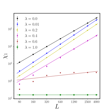
Figure 7: Plot of the finite size scaling for the susceptibility ($\chi_{1}$) at coupling $\lambda=0.0,0.01,0.2,0.4,0.6$, and $1.0$. The data (and the corresponding fits) have been vertically shifted to make all the fits in an order.

Appendix E Step Scaling Function

In order to argue that the traditional $XY$ model at the BKT transition and the two layer interacting dimer model are equivalent we compute the step scaling function (SSF) in both of them. We refer to the traditional $XY$ model defined through the lattice action

$$S=-\beta\sum_{\langle ij\rangle}\cos(\theta_{i}-\theta_{j}),$$ (19)

as the bosonic $XY$ model and dimer model defined in Eq. 10 as the fermionic $XY$ model. In order to compute the step-scaling function we first compute the second moment correlation length defined in a finite box of size $L$ using the expression

$$\xi(L)=\frac{1}{2\sin{(\pi/L)}}\sqrt{\frac{\chi}{F}-1},$$ (20)

where

$$\chi =\sum_{i}\langle{\cal O}^{+}_{i}{\cal O}^{-}_{0}\rangle,$$ (21)

$$F =\sum_{i}\langle{\cal O}^{+}_{i}{\cal O}^{-}_{0}\rangle\cos{(2\pi x/L)},$$ (22)

where $i=(x,t)$ is the space-time lattice site and ${\cal O}^{+}_{i},{\cal O}^{-}_{i}$ are lattice fields in the two lattice models. In the bosonic $XY$ model, ${\cal O}^{+}_{i}=e^{i\theta_{i}}$ and ${\cal O}^{-}_{i}=e^{-i\theta_{i}}$, while in the fermionic model ${\cal O}^{+}_{i}={\cal O}^{-}_{i}=\overline{\psi}_{i}\psi_{i}$.

The SSF for the bosonic $XY$ model is computed in the massive phase close to the critical point, for $\beta<\beta_{c}=1.1199$ [35]. To study the step scaling function, we prepare several pairs of data at $(\beta,L)$ and $(\beta,2L)$, and compute both $\xi(2L)/\xi(L)$ and $\xi(L)/L$ using the data presented in Fig. 9. We follow certain criteria as explained in [59], to ensure the minimization of finite volume and finite lattice spacing errors. In particular, we only choose lattices of sizes $L\geq L_{min}$, where $L_{min}=80$ for couplings $\beta\geq 0.92$. Since the correlation length increases for $\beta$ close to the $\beta_{c}$, larger lattice sizes are essential. The similar criteria for choosing the lattices sizes and couplings in the fermionic model is $L\geq L_{min}$, where $L_{min}=80$ for $0.62\leq\lambda\leq 0.9$, and $L_{min}=640$ for $\lambda<0.6$.

In order to compute the expectation value and error of $\xi(L)/L$, we use the jackknife analysis. We report the results here for the analysis with 40 jackknife blocks. The effect of variation of the jackknife blocks did not change the errors significantly, and were consistent with the errors obtained using a bootstrap analysis. In Fig. 8, we show an example of the variation of the average and error of $\xi(L)/L$ at $\lambda=0.353$ and $L=320$ for the fermionic model using both the jackknife and the bootstrap analysis as a function of block size. For both methods, we use the same number of block sizes, but in order to show the distinction between them, we have displaced the data on the x-axis by multiplying nBlock by a factor of 1.1 for the bootstrap analysis.

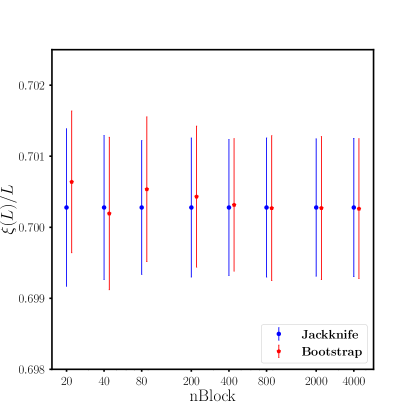
Figure 8: Error analysis of $\xi(L)/L$ at $\lambda=0.353$ and $L=320$ using both the jackknife and the bootstrap method. For the analysis, we have taken $12\times 10^{3}$ measurements, each averaged over $2\times 10^{3}$ values. In this plot, we used $20,40,80,200,400,800,2000$ and $4000$ block sizes.

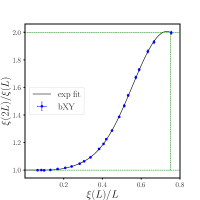
Figure 9: Plot of the step scaling function for the bosonic XY model superimposed with our data. The black line in the left plot is the function Eq. 23 with fit parameters from Table 4. In the right plot, the line shows the cubical spline interpolation.

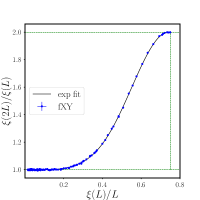
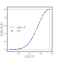
Figure 10: Plot of the step scaling function for the fermionic XY model superimposed with our data. The black line in the left plot is the function Eq. 23 with fit parameters from Table 4. In the right plot, the line shows the cubical spline interpolation.

In order to compare the SSF between the bosonic and the fermionic models we tried to parameterize the function in two different ways. In the first approach, we follow the idea discussed in [59] where it was proposed that

$$\Sigma(x)=1+{a_{1}}e^{-1/x}+{a_{2}}e^{-2/x}+{a_{3}}e^{-3/x}+{a_{4}}e^{-4/x},$$ (23)

where $x=\xi(L)/L$ and $\Sigma=\xi(2L)/\xi(L)$. The behavior of this function is such that, as $x\rightarrow 0$, the function $\Sigma(x)$ approaches 1. While this function is strictly valid only for small $x$ we find that this form fits our data well. The fit results are given in Table 4. We see that while we get good fits by including all four fit parameters, we can also fix $a_{2}=0$ and still get a good fits.

Range	$bXY$
$\xi(L)/L$	$a_{1}$	$a_{2}$	$a_{3}$	$a_{4}$	$\chi^{2}/DOF$
0.066-0.75	1.74(14)	-9(3)	236(24)	-649(51)	0.22
0.066-0.75	1.35(4)	-	171(5)	-513(17)	0.62
0.066-0.572	1.49(6)	-	135(15)	-321(81)	0.27
Range	$fXY$
$\xi(L)/L$	$a_{1}$	$a_{2}$	$a_{3}$	$a_{4}$	$\chi^{2}/DOF$
0.061-0.75	1.42(7)	2(2)	153(11)	-475(25)	0.48
0.061-0.75	1.48(2)	-	165(2)	-499(8)	0.50

Table 4: Values of $a_{1},a_{2},a_{3},a_{4}$ and $\chi^{2}/DOF$ obtained from the fit function $\Sigma(x)$ (defined in Eq. 23) for both the traditional $XY$ model and the fermionic $XY$ model.

In the second approach, to parameterize our SSF we used a cubical spline to interpolate the data. In Table 5, we provide a tabulation of the spline function that helps parameterize the SSF for both the bosonic and the fermionic models. The errors are obtained using a jackknife analysis.

	$bXY$	$fXY$		$bXY$	$fXY$
$\xi(L)/L$	$\xi(2L)/\xi(L)$	$\xi(2L)/\xi(L)$	$\xi(L)/L$	$\xi(2L)/\xi(L)$	$\xi(2L)/\xi(L)$
0.05	0.998(9)	1.000(5)	0.07	0.999(4)	1.002(2)
0.09	0.999(3)	1.002(4)	0.11	0.998(5)	1.002(4)
0.13	1.000(4)	1.002(4)	0.15	1.004(4)	1.003(2)
0.17	1.008(4)	1.006(4)	0.19	1.012(4)	1.011(4)
0.21	1.016(3)	1.016(4)	0.23	1.022(4)	1.020(3)
0.25	1.029(5)	1.026(1)	0.27	1.039(4)	1.037(2)
0.29	1.051(4)	1.053(3)	0.31	1.067(4)	1.069(2)
0.33	1.083(4)	1.087(2)	0.35	1.107(5)	1.111(4)
0.37	1.135(6)	1.136(4)	0.39	1.163(5)	1.167(6)
0.41	1.199(7)	1.206(6)	0.43	1.246(7)	1.254(3)
0.45	1.288(7)	1.308(7)	0.47	1.339(11)	1.365(9)
0.49	1.396(9)	1.423(11)	0.51	1.457(17)	1.481(12)
0.53	1.532(14)	1.539(8)	0.55	1.602(16)	1.595(6)
0.57	1.665(17)	1.661(8)	0.59	1.729(22)	1.724(7)
0.61	1.792(22)	1.783(7)	0.63	1.849(21)	1.842(8)
0.65	1.898(14)	1.890(5)	0.67	1.935(18)	1.927(5)
0.69	1.961(23)	1.957(9)	0.71	1.977(22)	1.985(6)
0.73	1.988(16)	1.999(6)	0.75	1.995(13)	1.999(12)

Table 5: Table of the step scaling function for both the bosonic and the fermionic $XY$ model.

In order to show how these two different parameterizations help capture our data we show the corresponding curves for the bosonic model in Fig. 9 and for the fermionic model in Fig. 10. We believe that a combined parameterization would best capture the true function. Hence, we use Eq. 23 for $\xi(L)/L\leq 0.572$ and the cubical spline interpolation for $\xi(L)/L\geq 0.572$. This combined form in the bosonic model is shown in Fig. 11, along with the bosonic model data. The dark line of this plot is used in the main paper to compare with the fermionic model.

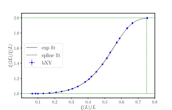
Figure 11: Plot of the step scaling function for the bosonic XY model using a combination of the exponential function and the spline function. In particular, we use Eq. 23 for $\xi(L)/L\leq 0.572$ (solid line), and the cubical spline interpolation for $\xi(L)/L\geq 0.572$ (dashed line). We use this plot in the main paper.

Appendix F Infinite Volume Correlation Length

We can compute the infinite volume correlation length $\xi_{\infty}$ using the SSF. Here we try to understand how $\xi_{\infty}$ depends on $\lambda$ in the fermionic $XY$ model. In order to reliably estimate the errors in $\xi_{\infty}$ we again use the jackknife analysis. We start with 40 jackknife blocks, where each block contains a pair ($\xi(L)/L$, $\xi(2L)/\xi(L)$) for different coupling values ($0.01\leq\lambda\leq 0.8$). We obtain 40 different cubical splines using each jackknife block. We then start with the initial $\xi(L)/L$ at $L=640$ in each block and evaluate $\xi(2^{n}L)$ using the spline function for arbitrary values of $n$, until the correlation length $\xi(2^{n}L)$ becomes insensitive to $L$. Finally, the jackknife mean and error is then computed from the 40 values. These results for $\xi_{\infty}$ and their errors are quoted in Table 6.

$\lambda$	$\xi_{\infty}$
0.3	145803(94882)
0.35	18275(1450)
0.4	4196(87)
0.45	1335(43)
0.5	538(6)
0.55	262(1)
0.6	144.9(5)
0.65	89(2)
0.7	59.38(23)
0.75	41.25(9)
0.8	30.54(12)

Table 6: Values of infinite volume correlation length for different couplings.

Since the correlation lengths increase exponentially as $\lambda$ becomes small, we were able to extract the infinite volume correlation length only in the range $0.3\leq\lambda\leq 0.8$. Below $\lambda<0.3$, our extrapolation methods fail.

Using the data in Table 6 we study the $\lambda$ dependence of $\xi_{\infty}$. For the bosonic $XY$ model, it is well known that as one approaches the BKT phase transition, the leading divergence of the infinite volume correlation length is captured by

$$\xi=C\exp\left(\frac{b}{\sqrt{\beta_{c}-\beta}}\right),$$ (24)

where $\beta_{c}$ is the critical coupling, and $b$ and $C$ are non-universal constants. For the fermionic $XY$ model since the partition function is an even function of $\lambda$ we expect $\xi_{\infty}$ to be a function of $\lambda^{2}$. Since the BKT critical point appears when $\lambda\rightarrow 0$, we conjecture that

$$\xi^{(1)}_{\infty}=a_{1}\exp\left(\frac{b_{1}}{\sqrt{\lambda^{2}}}\right).$$ (25)

We test this conjecture numerically by fitting the data in Table 6 to it. We also compare this to other fit forms including $\xi^{(2)}_{\infty}=a_{2}\exp(b_{2}/(\lambda^{2})^{1/4})$ and $\xi^{(3)}_{\infty}=a_{3}\exp(b_{3}/\sqrt{\lambda^{2}}+c_{3}\log(\lambda^{2})/2)$. The results are shown in Table 7. We observe that Eq. 25 is clearly quite good if we expect the constants $a$ and $b$ to be numbers which are not unnatural. We cannot rule out the presence of a power law correction to the expected form.

$i$	Range	$a_{i}$	$b_{i}$	$c_{i}$	${\chi}^{2}/DOF$
1	0.3-0.55	0.166(8)	4.049(26)	-	0.76
2	0.3-0.5	1e-5(3e-6)	12.35(13)	-	1.21
3	0.3-0.8	0.119(8)	4.68(8)	1.36(12)	1.15

Table 7: Values of $a_{1},b_{1},c_{1},a_{2},b_{2},a_{3},b_{3}$ and ${\chi}^{2}/DOF$ obtained from three different fit functions.

In Fig. 12, we show the data in Table 6 and the various fits. The first form is the expected behaviour from Eq. 25. The second form explores a possible dependence on square-root of $\lambda$ which is clearly unnatural. Finally the third form allows for a logarithmic correction in the exponential (which is equivalent to including a $1/\lambda$ dependence outside the exponential). We note that in this extended form the data in the larger range of $0.3\leq\lambda\leq 0.8$ can be fit.

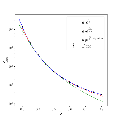
Figure 12: Plot of the infinite volume correlation length with coupling $\lambda$ for the fermionic $XY$ model together with several different functional forms. It seems that the correlation length increases exponentially with $\frac{1}{\lambda}$.

Appendix G Monte Carlo Results

We tabulate all of our Monte Carlo data in Tables 8, 9, 10, 11, 12, 13 and 14 for both the bosonic $XY$ and the fermionic $XY$ models, for various values of $L$ and couplings. The errors in these primary quantities have been obtained with 20 jackknife blocks.

$\lambda$	$L$	$\rho$	$\chi_{1}$	$F$	$\xi(L)$	$\Upsilon$
0.00	10	0	3.7294(17)	0.3318(3)	5.1774(32)	-
0.01	10	0.0001(0)	3.7308(8)	0.3312(3)	5.1836(24)	-
0.20	10	0.0280(0)	3.8439(12)	0.2847(3)	5.7207(38)	-
0.40	10	0.0698(0)	3.8385(12)	0.2488(3)	6.1466(40)	-
0.60	10	0.1165(0)	3.6879(14)	0.2319(2)	6.2470(39)	-
0.00	12	0	4.9365(18)	0.4431(6)	6.1519(53)	-
0.01	12	0.0001(0)	4.9415(15)	0.4437(3)	6.1511(21)	-
0.20	12	0.0288(0)	5.2022(16)	0.3684(5)	6.9979(55)	-
0.40	12	0.0701(0)	5.2157(14)	0.3247(4)	7.4981(52)	-
0.60	12	0.1171(0)	5.0057(21)	0.3069(3)	7.5585(50)	-
0.00	14	0	6.2486(26)	0.5667(6)	7.1146(50)	-
0.01	14	0.0002(0)	6.2558(23)	0.5664(6)	7.1216(43)	-
0.20	14	0.0290(0)	6.7316(31)	0.4579(6)	8.3168(61)	-
0.40	14	0.0703(0)	6.7761(23)	0.4065(6)	8.8942(74)	-
0.60	14	0.1175(0)	6.4768(21)	0.3907(5)	8.8683(58)	-
0.00	16	0	7.6612(35)	0.7005(10)	8.0789(72)	-
0.01	16	0.0002(0)	7.6729(30)	0.6975(8)	8.1047(62)	-
0.20	16	0.0292(0)	8.4206(32)	0.5513(6)	9.6832(60)	-
0.40	16	0.0704(0)	8.5034(29)	0.4948(8)	10.3112(88)	-
0.60	16	0.1177(0)	8.0952(34)	0.4834(7)	10.1705(84)	-
0.00	20	0	10.7423(47)	0.9926(11)	10.0173(69)	0.6058(2)
0.01	20	0.0002(0)	10.7770(53)	0.9853(9)	10.0758(54)	0.6071(4)
0.05	20	0.0044(0)	11.2088(48)	0.9162(8)	10.7130(62)	0.6203(2)
0.10	20	0.0119(0)	11.7235(59)	0.8370(12)	11.5272(109)	0.6255(7)
0.20	20	0.0293(0)	12.2905(37)	0.7525(11)	12.516(11)	0.6172(4)
0.30	20	0.0293(0)	12.2905(37)	0.7117(12)	12.9957(132)	0.6002(4)
0.40	20	0.0705(0)	12.4270(48)	0.6934(8)	13.1483(85)	0.5792(4)
0.50	20	0.0935(0)	12.1726(47)	0.6863(10)	13.0776(101)	0.5518(4)
0.60	20	0.1180(0)	11.7508(49)	0.6895(9)	12.8022(94)	0.5131(5)
0.70	20	0.1441(0)	11.1045(46)	0.7078(8)	12.2495(85)	0.4660(3)
0.80	20	0.1718(0)	10.2291(46)	0.7427(8)	11.4230(71)	0.4039(3)
1.00	20	0.2330(0)	7.7504(38)	-	-	0.2456(3)
0.00	22	0	12.4079(69)	1.1521(15)	10.9814(93)	-
0.01	22	0.0003(0)	12.4556(56)	1.1440(14)	11.0478(80)	-
0.20	22	0.0293(0)	14.4529(61)	0.8588(13)	13.978(13)	-
0.40	22	0.0705(0)	14.6262(56)	0.8008(14)	14.5986(142)	-
0.60	22	0.1182(0)	13.7526(67)	0.8092(8)	14.0516(94)	-
0.00	24	0	14.1467(70)	1.3157(13)	11.9626(81)	-
0.01	24	0.0003(0)	14.2197(72)	1.3055(14)	12.0483(81)	-
0.20	24	0.0293(0)	16.7707(98)	0.9749(14)	15.419(12)	-
0.40	24	0.0705(0)	16.9713(77)	0.9167(10)	16.031(12)	-
0.60	24	0.1182(0)	15.8922(78)	0.9313(14)	15.354(12)	-
0.00	26	0	15.9548(73)	1.4888(18)	12.9302(96)	-
0.01	26	0.0003(0)	16.0628(85)	1.4750(17)	13.0452(92)	-
0.20	26	0.0293(0)	19.2352(75)	1.0919(12)	16.909(10)	-
0.40	26	0.0706(0)	19.4497(68)	1.0370(16)	17.479(15)	-
0.60	26	0.1183(0)	18.149(11)	1.0657(13)	16.608(13)	-
0.00	28	0	17.844(11)	1.6689(22)	13.903(13)	-
0.01	28	0.0003(0)	17.996(7)	1.6558(17)	14.029(10)	-
0.20	28	0.0293(0)	21.841(11)	1.2127(24)	18.418(18)	-
0.40	28	0.0706(0)	22.090(12)	1.1668(18)	18.910(17)	-
0.60	28	0.1184(0)	20.527(9)	1.2049(19)	17.883(17)	-

Table 8: Results for $\rho$, $\chi_{1}$, $F$, $\chi(L)$ and $\Upsilon$ for the fermionic $XY$ model, $L=10$, $L=12$, $L=14$, $L=16$, $L=20$, $L=22$, $L=24$, $L=26$, and $L=28$.

$\lambda$	$L$	$\rho$	$\chi_{1}$	$F$	$\xi(L)$	$\Upsilon$
0.00	30	0	19.814(10)	1.8528(26)	14.893(13)	-
0.01	30	0.0004(0)	20.007(7)	1.8314(25)	15.069(13)	-
0.20	30	0.0293(0)	24.612(13)	1.3429(21)	19.911(17)	-
0.40	30	0.0706(0)	24.857(10)	1.3046(19)	20.324(18)	-
0.60	30	0.1184(0)	22.991(10)	1.3553(16)	19.112(13)	-
0.00	40	0	30.528(14)	2.883(4)	19.734(17)	0.6070(2)
0.01	40	0.0004(0)	31.221(15)	2.792(5)	20.335(22)	0.6141(5)
0.05	40	0.0049(0)	35.155(23)	2.364(3)	23.732(20)	0.6326(3)
0.10	40	0.0120(0)	37.847(16)	2.167(4)	25.861(27)	0.6290(7)
0.20	40	0.0293(0)	40.408(23)	2.068(4)	27.441(33)	0.6169(8)
0.30	40	0.0491(0)	41.066(17)	2.060(5)	27.728(39)	0.5990(4)
0.40	40	0.0707(0)	40.678(17)	2.084(4)	27.425(32)	0.5731(5)
0.50	40	0.0938(0)	39.311(18)	2.124(4)	26.668(24)	0.5354(6)
0.60	40	0.1186(0)	36.820(20)	2.207(3)	25.239(22)	0.4787(4)
0.70	40	0.1451(0)	33.059(15)	2.379(4)	22.885(21)	0.3998(4)
0.80	40	0.1736(0)	27.522(12)	2.644(3)	19.548(14)	0.2902(4)
1.00	40	0.2368(0)	13.879(11)	-	-	0.0741(2)
0.00	50	0	42.748(34)	4.054(7)	24.600(24)	-
0.01	50	0.0005(0)	42.381(38)	3.849(8)	25.841(34)	-
0.20	50	0.0293(0)	59.431(31)	2.929(5)	34.972(36)	-
0.40	50	0.0707(0)	59.612(25)	3.007(5)	34.547(31)	-
0.60	50	0.1187(0)	52.929(30)	3.262(4)	31.071(23)	-
0.00	60	0	56.226(41)	5.356(9)	29.442(30)	-
0.01	60	0.0005(0)	59.309(35)	4.957(9)	31.637(33)	-
0.20	60	0.0293(0)	81.534(35)	3.922(8)	42.502(50)	-
0.40	60	0.0707(0)	81.416(54)	4.078(8)	41.603(49)	-
0.60	60	0.1188(0)	70.941(38)	4.479(7)	36.801(30)	-
0.00	70	0	70.843(58)	6.767(11)	34.294(35)	-
0.01	70	0.0006(0)	76.153(55)	6.112(11)	37.728(47)	-
0.20	70	0.0293(0)	106.713(53)	5.023(11)	50.142(59)	-
0.40	70	0.0707(0)	105.919(52)	5.315(12)	48.486(64)	-
0.60	70	0.1188(0)	90.612(46)	5.915(10)	42.170(43)	-
0.00	80	0	86.610(70)	8.247(17)	39.257(44)	0.6067(3)
0.01	80	0.0006(0)	94.754(58)	7.322(16)	44.010(58)	0.6299(4)
0.05	80	0.0049(0)	114.924(74)	6.133(10)	53.637(51)	0.6336(4)
0.10	80	0.0120(0)	125.571(77)	6.104(15)	56.343(76)	0.6308(8)
0.20	80	0.0293(0)	134.390(89)	6.296(12)	57.445(63)	0.6149(7)
0.30	80	0.0491(0)	136.021(90)	6.476(15)	56.960(73)	0.5963(5)
0.40	80	0.0707(0)	133.220(76)	6.663(17)	55.505(75)	0.5639(7)
0.50	80	0.0940(0)	125.636(80)	6.959(13)	52.593(54)	0.5111(7)
0.60	80	0.1188(0)	111.685(68)	7.503(12)	47.457(43)	0.4239(6)
0.62	80	-	107.98(14)	7.67(3)	46.04(10)	-
0.64	80	-	103.64(13)	7.86(2)	44.45(8)	-
0.70	80	0.1457(0)	88.174(49)	8.618(10)	38.696(31)	0.2825(5)
0.80	80	0.1747(0)	56.099(43)	9.908(11)	27.499(22)	0.1190(3)
0.90	80	-	29.72(4)	9.74(1)	18.24(2)	-
1.00	80	0.2376(0)	15.851(15)	-	-	0.0039(1)
0.00	90	0	103.393(87)	9.829(19)	44.203(55)	-
0.01	90	0.0006(0)	115.008(71)	8.579(24)	50.461(82)	-
0.20	90	0.0293(0)	164.845(99)	7.676(19)	64.827(87)	-
0.40	90	0.0707(0)	162.88(10)	8.176(12)	62.322(60)	-
0.60	90	0.1189(0)	133.923(72)	9.304(18)	52.433(52)	-
0.00	100	0	121.10(13)	11.560(26)	49.001(64)	-
0.01	100	0.0006(0)	137.33(9)	9.822(17)	57.354(55)	-
0.20	100	0.0293(0)	197.89(14)	9.121(22)	72.42(10)	-
0.40	100	0.0707(0)	194.81(10)	9.774(19)	69.260(75)	-
0.60	100	0.1189(0)	157.38(13)	11.262(15)	57.337(57)	-

Table 9: Results for $\rho$, $\chi_{1}$, $F$, $\chi(L)$ and $\Upsilon$ for the fermionic $XY$ model, $L=30$, $L=40$, $L=50$, $L=60$, $L=70$, $L=80$, $L=90$, and $L=100$.

$\lambda$	$L$	$\rho$	$\chi_{1}$	$F$	$\xi(L)$	$\Upsilon$
0.00	110	0	139.51(12)	13.313(40)	53.91(10)	-
0.01	110	0.0006(0)	161.08(12)	11.108(28)	64.338(96)	-
0.20	110	0.0293(0)	233.79(15)	10.739(33)	79.80(13)	-
0.40	110	0.0707(0)	229.27(15)	11.500(19)	76.194(75)	-
0.60	110	0.1189(0)	181.84(13)	13.404(23)	62.070(70)	-
0.00	120	0	159.43(13)	15.189(32)	58.862(82)	-
0.01	120	0.0006(0)	186.01(17)	12.496(33)	71.18(12)	-
0.20	120	0.0293(0)	271.73(14)	12.447(37)	87.18(14)	-
0.40	120	0.0707(0)	265.92(20)	13.392(21)	82.945(84)	-
0.60	120	0.1189(0)	206.95(12)	15.726(23)	66.604(59)	-
0.00	130	0	179.47(19)	17.163(50)	63.63(12)	-
0.01	130	0.0006(0)	213.22(15)	13.849(46)	78.51(14)	-
0.20	130	0.0293(0)	312.66(17)	14.241(34)	94.72(18)	-
0.40	130	0.0707(0)	304.73(17)	15.346(32)	89.85(11)	-
0.60	130	0.1189(0)	231.93(20)	18.324(26)	70.647(75)	-
0.00	140	0	200.42(17)	19.13(5)	68.59(12)	-
0.01	140	0.0006(0)	241.54(22)	15.35(4)	85.53(12)	-
0.20	140	0.0293(0)	355.34(24)	16.11(4)	102.24(12)	-
0.40	140	0.0707(0)	346.00(18)	17.43(4)	96.74(12)	-
0.60	140	0.1190(0)	258.59(22)	20.90(3)	75.16(7)	-
0.00	150	0	222.47(26)	21.29(5)	73.40(10)	-
0.01	150	0.0006(0)	271.68(28)	16.82(5)	92.93(17)	-
0.20	150	0.0293(0)	400.88(24)	18.14(5)	109.68(19)	-
0.40	150	0.0707(0)	389.17(20)	19.64(3)	103.57(09)	-
0.60	150	0.1190(0)	285.22(24)	23.86(3)	79.02(08)	-
0.00	160	0	245.14(26)	23.54(6)	78.14(12)	0.6065(5)
0.01	160	0.0006(0)	302.95(28)	18.38(7)	100.20(22)	0.6353(6)
0.05	160	0.0049(0)	382.42(29)	17.88(5)	114.99(20)	0.6334(4)
0.10	160	0.0120(0)	419.42(25)	18.91(5)	117.20(18)	0.6301(8)
0.20	160	0.0293(0)	448.38(28)	20.30(4)	116.96(14)	0.6148(10)
0.30	160	0.0491(0)	450.15(30)	21.20(6)	114.56(19)	0.5913(6)
0.40	160	0.0707(0)	434.43(30)	21.96(5)	110.36(14)	0.5512(7)
0.50	160	0.0940(0)	393.80(17)	23.35(4)	101.44(10)	0.4753(7)
0.60	160	0.1190(0)	312.00(21)	26.86(5)	82.98(9)	0.3255(5)
0.62	160	-	287.38(24)	28.13(8)	77.31(12)	-
0.64	160	-	261.76(26)	29.35(9)	71.67(12)	-
0.65	160	-	247.46(18)	29.90(4)	68.70(7)	-
0.66	160	-	233.07(49)	30.33(10)	65.85(16)	-
0.70	160	0.1460(0)	175.85(13)	32.30(3)	53.69(5)	0.1111(5)
0.72	160	-	148.60(16)	32.65(8)	47.99(7)	-
0.75	160	-	113.48(11)	32.33(3)	40.35(3)	-
0.77	160	-	93.93(18)	31.47(7)	35.88(5)	-
0.80	160	0.1750(0)	71.25(7)	29.42(3)	30.37(3)	0.0116(2)
0.84	160	-	49.83(10)	25.83(4)	24.55(3)	-
0.86	160	-	42.23(7)	23.93(3)	22.27(4)	-
0.90	160	-	30.91(7)	20.26(3)	18.46(3)	-
1.00	160	0.2377(0)	15.92(1)	-	-	0
0.00	170	0	268.05(25)	25.71(6)	83.07(11)	-
0.01	170	0.0006(0)	336.4(2)	19.9(1)	107.92(24)	-
0.20	170	0.0293(0)	498.2(3)	22.6(1)	124.17(20)	-
0.40	170	0.0707(0)	480.9(3)	24.4(1)	117.08(15)	-
0.60	170	0.1190(0)	338.7(2)	30.3(1)	86.38(11)	-
0.00	240	0	450.53(58)	43.17(12)	117.34(19)	-
0.01	240	0.0006(0)	608.83(56)	32.19(10)	161.66(32)	-
0.20	240	0.0293(0)	908.26(71)	40.96(13)	175.78(30)	-
0.40	240	0.0707(0)	863.59(58)	44.60(96)	163.69(21)	-
0.60	240	0.1190(0)	520.76(45)	58.57(80)	107.31(13)	-

Table 10: Results for $\rho$, $\chi_{1}$, $F$, $\chi(L)$ and $\Upsilon$ for the fermionic $XY$ model, $L=110$, $L=120$, $L=130$, $L=140$, $L=150$, $L=160$, $L=170$, and $L=240$.

$\lambda$	$L$	$\rho$	$\chi_{1}$	$F$	$\xi(L)$	$\Upsilon$
0.00	320	0	693.32(77)	66.72(29)	156.07(37)	0.6060(8)
0.01	320	0.0006(0)	1003(1)	49.4(2)	223.69(62)	0.6367(4)
0.05	320	0.0049(0)	1281.02(69)	56.55(20)	236.98(47)	0.6342(4)
0.10	320	0.0120(0)	1406(1)	62.01(17)	237.14(36)	0.6284(10)
0.20	320	0.0293(0)	1497(1)	67.2(2)	234.96(48)	0.6156(9)
0.30	320	0.0491(0)	1492(1)	70.23(18)	229.17(35)	0.5869(9)
0.40	320	0.0707(0)	1403(1)	73.3(2)	216.97(33)	0.5349(7)
0.50	320	0.0940(0)	1187(1)	81.10(22)	188.08(32)	0.4158(6)
0.60	320	0.1190(0)	697.9(7)	101.8(1)	123.23(13)	0.1633(6)
0.65	320	-	408.76(49)	106.03(14)	86.06(9)	-
0.66	320	-	361.34(84)	104.91(25)	79.63(16)	-
0.70	320	0.1461(0)	218.49(33)	93.91(7)	58.66(6)	0.0097(2)
0.72	320	-	171.12(44)	85.57(17)	50.92(9)	-
0.75	320	-	121.13(15)	72.89(7)	41.44(4)	-
0.77	320	-	97.81(19)	64.54(9)	36.57(10)	-
0.80	320	0.1750(0)	72.25(6)	53.09(4)	30.59(3)	0.0001(0)
0.84	320	-	50.30(8)	40.76(6)	24.63(5)	-
0.86	320	-	42.33(8)	35.51(6)	22.32(4)	-
0.89	320	-	33.41(7)	29.19(5)	19.37(4)	-
0.90	320	-	31.05(7)	27.41(5)	18.55(5)	-
1.00	320	0.2376(0)	15.921(13)	-	-	0
0.00	640	0	1960(4)	186.98(78)	313.69(79)	0.6047(15)
0.01	640	0.0006(0)	3345(6)	151.9(8)	467(1)	0.6361(11)
0.05	640	0.0049(0)	4319(3)	186.63(68)	479.29(97)	0.6328(9)
0.10	640	0.0120(0)	4724(5)	208.09(74)	474.52(92)	0.6267(14)
0.20	640	0.0293(0)	5002(4)	224.3(9)	470(1)	0.6152(9)
0.30	640	0.0491(0)	4919(5)	234.20(80)	455.58(91)	0.5818(12)
0.40	640	0.0707(0)	4493(3)	245.6(6)	423.63(64)	0.5098(8)
0.45	640	-	4038(4)	261.03(75)	387.45(66)	-
0.50	640	0.0940(0)	3263(2)	293.12(76)	324.25(52)	0.3101(10)
0.55	640	-	2087(3)	340.57(53)	230.68(26)	-
0.60	640	0.1191(0)	994(1)	332.0(4)	143.53(14)	0.0259(3)
0.70	640	0.1461(0)	221.05(31)	165.49(17)	59.02(6)	0
0.80	640	0.1750(0)	72.36 (7)	66.37(6)	30.60(3)	0
0.84	640	-	50.11(8)	47.33(7)	24.68(4)	-
0.89	640	-	33.44(6)	32.28(5)	19.38(4)	-
0.90	640	-	31.04(6)	30.04(5)	18.55(4)	-
1.00	640	0.2377(0)	15.905(12)	-	-	0

Table 11: Results for $\rho$, $\chi_{1}$, $F$, $\chi(L)$ and $\Upsilon$ for the fermionic $XY$ model, $L=320$ and $L=640$.

$\lambda$	$L$	$\rho$	$\chi_{1}$	$F$	$\xi(L)$	$\Upsilon$
0.00	1280	0	5531(13)	527(3)	628(2)	0.6073(14)
0.01	1280	0.0006(0)	11264(14)	486(3)	959(4)	0.6363(16)
0.05	1280	0.0049(0)	14466(15)	628(3)	955(3)	0.6348(11)
0.10	1280	0.0120(0)	15839(11)	696(3)	949(2)	0.6281(12)
0.20	1280	0.0293(0)	16702(15)	750(4)	939(2)	0.6113(12)
0.25	1280	-	16620(17)	773(2)	922(2)	-
0.30	1280	0.0491(0)	16239(16)	782(3)	905(1)	0.5772(8)
0.35	1280	-	15466(12)	796(2)	874(1)	-
0.40	1280	0.0707(0)	14072(14)	836(2)	810(1)	0.4736(7)
0.45	1280	-	11510(13)	934(2)	686(1)	-
0.50	1280	0.0940(0)	7038(10)	1110(2)	470(0)	0.1443(9)
0.60	1280	0.1191(0)	1031(2)	683(1)	145.51(24)	0.0004(1)
0.70	1280	0.1461(0)	220.98(27)	203.90(24)	58.96(8)	0
0.80	1280	0.1750(0)	72.28(7)	70.68(7)	30.60(3)	0
0.90	1280	-	30.92(6)	30.67(6)	18.49(5)	-
1.00	1280	0.2377(0)	15.924(11)	-	-	0
0.00	2560	0	15726(52)	1513(15)	1249(8)	0.6055(19)
0.01	2560	0.0006(0)	37802(51)	1632(8)	1918(5)	0.6363(14)
0.05	2560	0.0049(0)	48750(66)	2090(10)	1924(4)	0.6333(15)
0.10	2560	0.0120(0)	53240(59)	2317(11)	1909(5)	0.6292(13)
0.20	2560	0.0293(0)	55722(75)	2506(10)	1877(4)	0.6108(14)
0.25	2560	-	55081(64)	2574(15)	1840(6)	-
0.30	2560	0.0491(0)	53348(50)	2616(8)	1793(3)	0.5685(9)
0.35	2560	-	49684(68)	2693(11)	1702(4)	-
0.40	2560	0.0707(0)	42416(50)	2914(11)	1499(3)	0.4139(11)
0.45	2560	-	27460(41)	3503(10)	1065(2)	-
0.50	2560	0.0940(0)	9492(16)	3496(3)	533(0)	0.0182(3)
0.60	2560	0.1191(0)	1027(1)	912(1)	144.92(25)	0
0.70	2560	0.1461(0)	221.19(24)	216.63(23)	59.10(8)	0
0.80	2560	0.1750(0)	72.26(8)	71.85(8)	30.53(3)	0
0.90	2560	-	30.95(5)	30.88(5)	18.51(4)	-
1.00	2560	0.2376(0)	15.932(15)	-	-	0
0.00	4000	0	30823(168)	-	-	-
0.01	4000	0.0006(0)	82478(194)	-	-	-
0.05	4000	0.0049(0)	106095(224)	-	-	-
0.1	4000	0.0120(0)	116173(157)	-	-	-
0.2	4000	0.0293(0)	121218(115)	-	-	-
0.3	4000	0.0491(0)	114403(155)	-	-	-
0.4	4000	0.0707(0)	82579(121)	-	-	-
0.5	4000	0.0940(0)	9743(19)	-	-	-
0.6	4000	0.1191(0)	1033(2)	-	-	-
0.7	4000	0.1461(0)	221.21(25)	-	-	-
0.8	4000	0.1750(0)	72.07(9)	-	-	-
1.0	4000	0.2376(1)	15.93(2)	-	-	-

Table 12: Results for $\rho$, $\chi_{1}$, $F$, $\chi(L)$ and $\Upsilon$ for the fermionic $XY$ model, $L=1280$, $L=2560$ and $L=4000$.

	$L=40$			$L=80$			$L=160$
$\beta$	$\chi$	$F$	$\xi(L)$	$\chi$	$F$	$\xi(L)$	$\chi$	$F$	$\xi(L)$
0.920	152.51(43)	42.32(11)	10.28(2)	162.85(32)	96.69(14)	10.54(2)	163.07(34)	139.21(29)	10.54(3)
0.940	210.23(52)	42.59(10)	12.64(2)	248.43(69)	116.73(27)	13.53(3)	250.93(76)	195.02(47)	13.64(4)
0.955	263.59(58)	41.09(12)	14.83(4)	354(1)	130.41(32)	16.68(4)	364(1)	252.31(63)	16.94(5)
0.975	338.59(71)	38.39(14)	17.82(5)	581(1)	139.79(44)	22.62(6)	647(2)	347(1)	23.67(8)
0.980	359.02(60)	37.72(12)	18.60(3)	658(2)	140.37(34)	24.46(6)	759(2)	371.54(87)	26.01(6)
0.985	378.60(77)	36.66(17)	19.46(5)	735(2)	138.42(44)	26.45(7)	895(3)	397.05(99)	28.51(9)
0.990	395.35(67)	36.09(15)	20.11(6)	820(1)	137.25(35)	28.41(6)	1069(4)	418(1)	31.79(10)
0.995	411.92(88)	35.16(15)	20.86(6)	911(2)	134.31(41)	30.62(7)	1276(4)	437(1)	35.32(10)
1.000	428.89(71)	34.46(16)	21.56(6)	999(2)	130.56(51)	32.85(8)	1532(4)	454(2)	39.25(14)
1.010	459.68(93)	33.00(14)	22.91(7)	1181(3)	123.96(46)	37.18(9)	2158(7)	461(1)	48.89(13)
1.015	474.58(62)	32.37(21)	23.55(8)	1270(3)	121.18(67)	39.21(14)	2539(9)	460(1)	54.16(14)
1.024	500.46(56)	31.71(12)	24.50(5)	1416(2)	114.09(60)	43.02(12)	3280(12)	437(1)	64.93(23)
1.026	505.80(56)	31.22(11)	24.85(5)	1443(4)	112.83(61)	43.73(16)	3454(8)	433(2)	67.23(16)
1.030	515.03(68)	30.74(13)	25.29(7)	1499(2)	110.99(46)	45.03(10)	3771(9)	420(2)	71.91(20)
1.035	526(1)	30.14(15)	25.86(9)	1569(3)	108.42(47)	46.74(11)	4162(8)	402(2)	77.85(24)
1.064	586.41(74)	28.22(14)	28.34(9)	1891(3)	97.25(74)	54.70(24)	5935(10)	342(3)	103.02(55)
1.066	591.16(64)	27.83(21)	28.67(12)	1907(3)	97.54(53)	54.86(17)	6034(10)	332(2)	105.48(45)
1.070	597.61(69)	27.64(18)	28.94(10)	1944(2)	97.22(56)	55.50(17)	6221(13)	334(2)	106.96(36)
1.078	609.68(72)	27.84(11)	29.13(7)	2007(2)	94.37(52)	57.33(17)	6562(10)	323(2)	111.99(44)
1.084	620.71(96)	27.50(10)	29.60(6)	2050(4)	93.65(67)	58.22(23)	6731(12)	322(2)	113.60(45)
1.104	648.64(76)	26.54(16)	30.86(10)	2184(3)	91.11(64)	61.04(25)	7343(11)	313(2)	120.78(42)
1.111	659(1)	26.40(22)	31.21(15)	2233(4)	90.99(89)	61.79(33)	7531(15)	310(3)	122.85(76)

Table 13: Results for $\chi$, $F$ and $\chi(L)$ for the bosonic $XY$ model, $L=40$, $L=80$, and $L=160$.

	$L=320$			$L=640$			$L=1280$
$\beta$	$\chi$	$F$	$\xi(L)$	$\chi$	$F$	$\xi(L)$	$\chi$	$F$	$\xi(L)$
0.920	162.08(49)	155.43(45)	10.53(4)	162.71(42)	160.99(41)	10.54(3)	161(2)	160(2)	10.53(6)
0.940	251.67(39)	234.84(36)	13.63(4)	251.09(66)	246.70(65)	13.59(3)	249(2)	248(2)	13.59(6)
0.955	364(1)	328(1)	16.88(5)	363(1)	353(1)	16.81(7)	360(3)	358(2)	16.77(5)
0.975	645(2)	531(2)	23.59(8)	652(2)	618(1)	23.66(8)	647(2)	639(2)	23.44(8)
0.980	767(2)	609(1)	26.03(7)	765(2)	718(2)	26.16(9)	766(3)	753(3)	26.13(10)
0.985	909(3)	691(1)	28.61(12)	906(2)	840(2)	28.63(9)	909(3)	891(3)	28.72(10)
0.990	1086(3)	780(2)	31.91(8)	1083(3)	986(2)	31.85(14)	1091(4)	1065(4)	31.76(14)
0.995	1308(5)	876(3)	35.74(11)	1321(6)	1176(6)	35.78(14)	1313(5)	1274(5)	35.52(14)
1.000	1609(5)	994(2)	40.07(10)	1612(6)	1396(4)	40.12(17)	1605(5)	1546(4)	39.91(14)
1.010	2479(10)	1227(3)	51.44(17)	2510(8)	1993(5)	51.90(19)	2498(8)	2346(7)	51.85(28)
1.015	3182(13)	1354(4)	59.16(16)	3220(14)	2392(8)	59.93(27)	3200(13)	2943(11)	60.15(24)
1.024	493116)	1494(5)	77.24(19)	5204(14)	3241(10)	79.26(32)	5257(30)	4564(22)	79.41(36)
1.026	5465(18)	1513(5)	82.30(29)	5834(28)	3455(11)	84.52(36)	5878(19)	5013(17)	84.64(24)
1.030	6660(22)	1549(6)	92.52(27)	7439(36)	3893(11)	97.23(43)	7499(34)	6092(23)	97.89(36)
1.035	8342(34)	1520(8)	107.90(34)	10258(48)	4422(17)	117.01(49)	10447(36)	7807(23)	118.46(38)
1.064	18032(36)	1187(8)	191.87(73)	49738(162)	4371(35)	328(1)	108892(596)	16547(126)	481(2)
1.066	18469(44)	1185(8)	194.64(80)	52457(122)	4299(30)	341(1)	124091(744)	16207(149)	526(4)
1.070	19466(43)	1176(7)	200.89(66)	57232(180)	4110(25)	366(2)	151071(649)	15152(146)	612(4)
1.078	20924(52)	1112(9)	214.95(95)	65456(205)	3877(31)	406(2)	197058(841)	13360(128)	755(4)
1.084	21967(47)	1103(9)	221(1)	70376(200)	3802(23)	426(2)	221594(633)	12822(111)	822(4)
1.104	24538(58)	1048(7)	241(1)	82560(241)	3582(29)	478(2)	274700(716)	12070(122)	950(6)
1.111	25340(56)	1062(10)	243(1)	85517(263)	3617(41)	485(3)	288454(1069)	12234(164)	968(7)

Table 14: Results for $\chi$, $F$ and $\chi(L)$ for the bosonic $XY$ model, $L=320$, $L=640$ and $L=1280$.

References

- Wilson [1983] K. G. Wilson, The renormalization group and critical phenomena, Rev. Mod. Phys. 55, 583 (1983).
- Klco and Savage [2019] N. Klco and M. J. Savage, Digitization of scalar fields for quantum computing, Phys. Rev. A 99, 052335 (2019), arXiv:1808.10378 [quant-ph] .
- Alexandru et al. [2019] A. Alexandru, P. F. Bedaque, H. Lamm, and S. Lawrence (NuQS), Models on Quantum Computers, Phys. Rev. Lett. 123, 090501 (2019), arXiv:1903.06577 [hep-lat] .
- Singh and Chandrasekharan [2019] H. Singh and S. Chandrasekharan, Qubit regularization of the sigma model, Phys. Rev. D 100, 054505 (2019), arXiv:1905.13204 [hep-lat] .
- Bañuls et al. [2020] M. C. Bañuls et al., Simulating Lattice Gauge Theories within Quantum Technologies, Eur. Phys. J. D 74, 165 (2020), arXiv:1911.00003 [quant-ph] .
- Zache et al. [2022] T. V. Zache, M. Van Damme, J. C. Halimeh, P. Hauke, and D. Banerjee, Toward the continuum limit of a D quantum link Schwinger model, Phys. Rev. D 106, L091502 (2022), arXiv:2104.00025 [hep-lat] .
- Ciavarella et al. [2021] A. Ciavarella, N. Klco, and M. J. Savage, Trailhead for quantum simulation of SU(3) Yang-Mills lattice gauge theory in the local multiplet basis, Phys. Rev. D 103, 094501 (2021), arXiv:2101.10227 [quant-ph] .
- Mariani et al. [2023] A. Mariani, S. Pradhan, and E. Ercolessi, Hamiltonians and gauge-invariant Hilbert space for lattice Yang-Mills-like theories with finite gauge group, arXiv:2301.12224 (2023), arXiv:2301.12224 [quant-ph] .
- Zache et al. [2023] T. V. Zache, D. Gonzalez-Cuadra, and P. Zoller, Quantum and classical spin network algorithms for -deformed Kogut-Susskind gauge theories, arXiv:2304.02527 (2023).
- Hayata and Hidaka [2023] T. Hayata and Y. Hidaka, String-net formulation of Hamiltonian lattice Yang-Mills theories and quantum many-body scars in a nonabelian gauge theory, arXiv:2305.05950 (2023), arXiv:2305.05950 [hep-lat] .
- Wiese [1999] U. J. Wiese, Quantum spins and quantum links: The D theory approach to field theory, Nucl. Phys. B Proc. Suppl. 73, 146 (1999), arXiv:hep-lat/9811025 .
- Brower et al. [2004] R. Brower, S. Chandrasekharan, S. Riederer, and U. J. Wiese, D theory: Field quantization by dimensional reduction of discrete variables, Nucl. Phys. B 693, 149 (2004), arXiv:hep-lat/0309182 .
- Banerjee et al. [2013] D. Banerjee, M. Bögli, M. Dalmonte, E. Rico, P. Stebler, U. J. Wiese, and P. Zoller, Atomic Quantum Simulation of U(N) and SU(N) Non-Abelian Lattice Gauge Theories, Phys. Rev. Lett. 110, 125303 (2013), arXiv:1211.2242 [cond-mat.quant-gas] .
- Wiese [2021] U.-J. Wiese, From quantum link models to D-theory: a resource efficient framework for the quantum simulation and computation of gauge theories, Phil. Trans. A. Math. Phys. Eng. Sci. 380, 20210068 (2021), arXiv:2107.09335 [hep-lat] .
- Sachdev [2011] S. Sachdev, Quantum Phase Transitions, 2nd ed. (Cambridge University Press, 2011).
- Affleck and Haldane [1987] I. Affleck and F. D. M. Haldane, Critical Theory of Quantum Spin Chains, Phys. Rev. B 36, 5291 (1987).
- Senthil et al. [2004] T. Senthil, L. Balents, S. Sachdev, A. Vishwanath, and M. P. A. Fisher, Quantum criticality beyond the landau-ginzburg-wilson paradigm, Phys. Rev. B 70, 144407 (2004).
- Banerjee et al. [2019] D. Banerjee, S. Chandrasekharan, D. Orlando, and S. Reffert, Conformal dimensions in the large charge sectors at the O(4) Wilson-Fisher fixed point, Phys. Rev. Lett. 123, 051603 (2019), arXiv:1902.09542 [hep-lat] .
- Singh [2022] H. Singh, Qubit regularized O(N) nonlinear sigma models, Phys. Rev. D 105, 114509 (2022), arXiv:1911.12353 [hep-lat] .
- Nahum et al. [2011] A. Nahum, J. T. Chalker, P. Serna, M. Ortuno, and A. M. Somoza, 3D loop models and the sigma model, Phys. Rev. Lett. 107, 110601 (2011), arXiv:1104.4096 [cond-mat.stat-mech] .
- Nahum et al. [2013] A. Nahum, P. Serna, A. M. Somoza, and M. Ortuño, Loop models with crossings, Phys. Rev. B 87, 184204 (2013), arXiv:1303.2342 [cond-mat.stat-mech] .
- Nahum et al. [2015] A. Nahum, J. T. Chalker, P. Serna, M. Ortuño, and A. M. Somoza, Deconfined Quantum Criticality, Scaling Violations, and Classical Loop Models, Phys. Rev. X 5, 041048 (2015), arXiv:1506.06798 [cond-mat.str-el] .
- Alet et al. [2006] F. Alet, Y. Ikhlef, J. L. Jacobsen, G. Misguich, and V. Pasquier, Classical dimers with aligning interactions on the square lattice, Phys. Rev. E 74, 041124 (2006).
- Kundu and Damle [2023] S. Kundu and K. Damle, Flux fractionalization transition in two-dimensional dimer-loop models (2023), arXiv:2305.07012 [cond-mat.stat-mech] .
- Bietenholz et al. [2003] W. Bietenholz, A. Gfeller, and U. J. Wiese, Dimensional reduction of fermions in brane worlds of the Gross-Neveu model, JHEP 10, 018, arXiv:hep-th/0309162 .
- Beard et al. [2005] B. B. Beard, M. Pepe, S. Riederer, and U. J. Wiese, Study of CP(N-1) theta-vacua by cluster-simulation of SU(N) quantum spin ladders, Phys. Rev. Lett. 94, 010603 (2005), arXiv:hep-lat/0406040 .
- Laflamme et al. [2016] C. Laflamme, W. Evans, M. Dalmonte, U. Gerber, H. Mejía-Díaz, W. Bietenholz, U. J. Wiese, and P. Zoller, P(N1) quantum field theories with alkaline-earth atoms in optical lattices, Annals Phys. 370, 117 (2016), arXiv:1507.06788 [quant-ph] .
- Caspar and Singh [2022] S. Caspar and H. Singh, From Asymptotic Freedom to Vacua: Qubit Embeddings of the O(3) Nonlinear Model, Phys. Rev. Lett. 129, 022003 (2022), arXiv:2203.15766 [hep-lat] .
- Zhou et al. [2022] J. Zhou, H. Singh, T. Bhattacharya, S. Chandrasekharan, and R. Gupta, Spacetime symmetric qubit regularization of the asymptotically free two-dimensional O(4) model, Phys. Rev. D 105, 054510 (2022), arXiv:2111.13780 [hep-lat] .
- Bhattacharya et al. [2021] T. Bhattacharya, A. J. Buser, S. Chandrasekharan, R. Gupta, and H. Singh, Qubit regularization of asymptotic freedom, Phys. Rev. Lett. 126, 172001 (2021), arXiv:2012.02153 [hep-lat] .
- Berezinsky [1971] V. L. Berezinsky, Destruction of long range order in one-dimensional and two-dimensional systems having a continuous symmetry group. I. Classical systems, Sov. Phys. JETP 32, 493 (1971).
- Kosterlitz and Thouless [1973] J. M. Kosterlitz and D. J. Thouless, Ordering, metastability and phase transitions in two-dimensional systems, J. Phys. C 6, 1181 (1973).
- Kenna and Irving [1997] R. Kenna and A. C. Irving, The Kosterlitz-Thouless universality class, Nucl. Phys. B 485, 583 (1997), arXiv:hep-lat/9601029 .
- Stamper-Kurn and Ueda [2013] D. M. Stamper-Kurn and M. Ueda, Spinor bose gases: Symmetries, magnetism, and quantum dynamics, Rev. Mod. Phys. 85, 1191 (2013).
- Hasenbusch [2005] M. Hasenbusch, The Two dimensional XY model at the transition temperature: A High precision Monte Carlo study, J. Phys. A 38, 5869 (2005), arXiv:cond-mat/0502556 .
- Hasenbusch [2006] M. Hasenbusch, The Three-dimensional XY universality class: A High precision Monte Carlo estimate of the universal amplitude ratio A+ / A-, J. Stat. Mech. 0608, P08019 (2006), arXiv:cond-mat/0607189 .
- José et al. [1977] J. V. José, L. P. Kadanoff, S. Kirkpatrick, and D. R. Nelson, Renormalization, vortices, and symmetry-breaking perturbations in the two-dimensional planar model, Phys. Rev. B 16, 1217 (1977).
- Bietenholz et al. [2013] W. Bietenholz, M. Bögli, F. Niedermayer, M. Pepe, F. G. Rejon-Barrera, and U. J. Wiese, Topological Lattice Actions for the 2d XY Model, JHEP 03, 141, arXiv:1212.0579 [hep-lat] .
- Zinn-Justin [2002] J. Zinn-Justin, Quantum Field Theory and Critical Phenomena (Oxford University Press, 2002).
- Zhang et al. [2021] J. Zhang, Y. Meurice, and S.-W. Tsai, Truncation effects in the charge representation of the O(2) model, Phys. Rev. B 103, 245137 (2021), arXiv:2104.06342 [cond-mat.quant-gas] .
- Chen et al. [2003] W. Chen, K. Hida, and B. C. Sanctuary, Ground-state phase diagram of chains with uniaxial single-ion-type anisotropy, Phys. Rev. B 67, 104401 (2003).
- Banerjee and Chandrasekharan [2010] D. Banerjee and S. Chandrasekharan, Finite size effects in the presence of a chemical potential: A study in the classical non-linear O(2) sigma-model, Phys. Rev. D 81, 125007 (2010), arXiv:1001.3648 [hep-lat] .
- [43] The model introduced in [4], that did not contain two site loops between neighboring sites, was studied in dimensions by Hersh Singh, but the results were not published since the BKT transition required fine-tuning as usual.
- Ayyar and Chandrasekharan [2015] V. Ayyar and S. Chandrasekharan, Massive fermions without fermion bilinear condensates, Phys. Rev. D 91, 065035 (2015), arXiv:1410.6474 [hep-lat] .
- Ayyar and Chandrasekharan [2016] V. Ayyar and S. Chandrasekharan, Origin of fermion masses without spontaneous symmetry breaking, Phys. Rev. D 93, 081701 (2016), arXiv:1511.09071 [hep-lat] .
- Maiti et al. [2022] S. Maiti, D. Banerjee, S. Chandrasekharan, and M. K. Marinkovic, Three-dimensional Gross-Neveu model with two flavors of staggered fermions, PoS LATTICE2021, 510 (2022), arXiv:2111.15134 [hep-lat] .
- Chandrasekharan [2010] S. Chandrasekharan, Fermion bag approach to lattice field theories, Phys. Rev. D 82, 025007 (2010).
- [48] For more details please see the supplementary material attached.
- Adams and Chandrasekharan [2003] D. H. Adams and S. Chandrasekharan, Chiral limit of strongly coupled lattice gauge theories, Nucl. Phys. B 662, 220 (2003), arXiv:hep-lat/0303003 .
- Kasteleyn [1963] P. W. Kasteleyn, Dimer statistics and phase transitions, Journal of Mathematical Physics 4, 287 (1963), https://doi.org/10.1063/1.1703953 .
- Fisher [1961] M. E. Fisher, Statistical mechanics of dimers on a plane lattice, Phys. Rev. 124, 1664 (1961).
- Fisher and Stephenson [1963] M. E. Fisher and J. Stephenson, Statistical mechanics of dimers on a plane lattice. ii. dimer correlations and monomers, Phys. Rev. 132, 1411 (1963).
- Allegra [2015] N. Allegra, Exact solution of the 2d dimer model: Corner free energy, correlation functions and combinatorics, Nuclear Physics B 894, 685 (2015).
- Chandrasekharan and Strouthos [2003] S. Chandrasekharan and C. G. Strouthos, Kosterlitz-thouless universality in dimer models, Phys. Rev. D 68, 091502 (2003).
- Wilkins and Powell [2020] N. Wilkins and S. Powell, Interacting double dimer model on the square lattice, Phys. Rev. B 102, 174431 (2020).
- Desai et al. [2021] N. Desai, S. Pujari, and K. Damle, Bilayer coulomb phase of two-dimensional dimer models: Absence of power-law columnar order, Phys. Rev. E 103, 042136 (2021).
- Balog [2001] J. Balog, Kosterlitz-Thouless theory and lattice artifacts, J. Phys. A 34, 5237 (2001), arXiv:hep-lat/0011078 .
- Balog et al. [2001] J. Balog, M. Niedermaier, F. Niedermayer, A. Patrascioiu, E. Seiler, and P. Weisz, Does the XY model have an integrable continuum limit?, Nucl. Phys. B 618, 315 (2001), arXiv:hep-lat/0106015 .
- Caracciolo et al. [1995] S. Caracciolo, R. G. Edwards, A. Pelissetto, and A. D. Sokal, Asymptotic scaling in the two-dimensional 0(3) sigma model at correlation length 10**5, Phys. Rev. Lett. 75, 1891 (1995), arXiv:hep-lat/9411009 .