Self-Distilled Quantization: Achieving High Compression Rates in Transformer-Based Language Models

Abstract

We investigate the effects of post-training quantization and quantization-aware training on the generalization of Transformer language models. We present a new method called self-distilled quantization (SDQ) that minimizes accumulative quantization errors and outperforms baselines. We apply SDQ to multilingual models XLM-R${}_{\text{Base}}$ and InfoXLM${}_{\text{Base}}$ and demonstrate that both models can be reduced from 32-bit floating point weights to 8-bit integer weights while maintaining a high level of performance on the XGLUE benchmark. Our results also highlight the challenges of quantizing multilingual models, which must generalize to languages they were not fine-tuned on.

1 Introduction

A main aim of neural network quantization is to reduce the size and computational demands of a model while maintaining its performance. There are two main approaches: quantization-aware training (QAT) Banner et al. (2018); Chin et al. (2020); Faghri et al. (2020); Kim et al. (2020); Wang et al. (2018) and post-training quantization (PTQ) Neill (2020); Bondarenko et al. (2021); Kim et al. (2021); Dettmers et al. (2022). Both of these approaches have limitations in terms of dealing with accumulative quantization errors that are propogated within the layers of a neural network during the forward pass Zhao et al. (2019); Fan et al. (2020). To address this issue, we propose a method called Self-Distilled Quantization (SDQ) that combines self-attention and output distillation with quantization to compress large language models. SDQ involves injecting quantization noise into the student network during training and distilling knowledge from a fine-tuned teacher network from both its final output and outputs of intermediate self-attention layers. By distilling knowledge of the self-attention layers, as depicted in Figure 1, we further reduce the compounding effect of quantization errors in the network. We use SDQ for self-attention models and demonstrate its effectiveness in compressing multilingual models XLM-R${}_{\text{Base}}$ and InfoXLM${}_{\text{Base}}$, achieving high compression rates while maintaining performance on the XGLUE benchmark. Lastly, we identify that quantization error is largest at the output of self-attention modules.

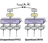
Figure 1: Self-Attention Self-Distilled Quantization

2 Related Work

Combining quantization and distillation has been previously explored by Mishra and Marr (2017), who used three different schemes to combine low bit precision and knowledge distillation (KD) using a 4-bit ResNet network. Polino et al. (2018) used a distillation loss with respect to a quantized teacher network to train a student network, and also proposed differentiable quantization, which optimizes the location of quantization points through SGD. Zhou et al. (2017) used iterative quantization, supervised by a teacher network, to retrain an FP-32 model with low precision convolution weights (binary, ternary, and 4 bits). Kim et al. (2019) used QAT and fine-tuning to mitigate the regularization effect of KD on quantized models. Q8BERT Zafrir et al. (2019) and fully Quantized Transformer Prato et al. (2019) applied QAT with the Straight-Through Estimator to approximate non-differentiable quantization in INT-8 format. We now describe the methodology of SDQ.

3 Methodology

We begin by defining a dataset $\mathcal{D}:=\{(X_{i},y_{i})\}^{D}_{i=1}$ with samples $s_{i}=(X_{i},\bm{y}_{i})$, where each $X_{i}:=(\bm{x}_{1},\ldots,\bm{x}_{N})$ and $\bm{x}_{i}\in\mathbb{R}^{d}$ is the $i$-th vector. For structured prediction $y_{i}\in\{0,1\}^{N\times d_{y}}$ and for single and pairwise sentence classification, $y_{i}\in\{0,1\}^{d_{y}}$, where $d_{y}$ is the number of classes. Let $\bm{y}^{S}=f_{\theta}(X_{i})$ be the output prediction ($y^{S}\in\mathbb{R}^{d_{y}}$) from the student $f_{\theta}(\cdot)$ with pretrained parameters $\theta:=\{\text{\bf W}_{l},\bm{b}_{l}\}_{l=1}^{L}$ for $L$ layers and the outputs of self-attention blocks are denoted as $\bm{A}_{l}$. The loss function for standard classification fine-tuning is defined as the cross-entropy loss $\ell_{CE}(\bm{y}^{S},\bm{y})$.

Self-Distilled Quantization

For self-distilled quantization, we also require a fine-tuned teacher network $f_{\Theta}$, that has been tuned from the pretrained state $f_{\theta}$, to retrieve the soft teacher labels $y^{T}:=f_{\Theta}(\bm{x})$, where $y^{T}\in\mathbb{R}^{C}$ and $\sum_{c}^{C}y^{T}_{c}=1$. The soft label $\bm{y}^{T}$ can be more informative than the one-hot targets $\bm{y}$ used for standard classification as they implicitly approximate pairwise class similarities through logit probabilities. The Kullbeck-Leibler divergence (KLD) $\ell_{\mathrm{KLD}}$ is then used with the main task cross-entropy loss $\ell_{CE}$ to express $\ell_{\mathrm{SDQ}_{\text{KLD}}}$ as shown in Equation 2,

$$\begin{split}\ell_{\mathrm{SDQ}_{\text{KLD}}}\text{=}\,\ell_{\mathrm{CE}}(\bm{y}^{S},\bm{y})\text{+}\alpha\tau^{2}D_{\mathrm{KLD}}\big{(}\bm{y}^{S},\bm{y}^{T}\big{)}\end{split}$$ (1)

where $D_{\mathrm{KLD}}(\bm{y}^{S},\bm{y}^{T})=\mathbb{H}(\bm{y}^{T})-\bm{y}^{T}\log(\bm{y}^{S})$, $\mathbb{H}(\bm{y}^{T})=\bm{y}^{T}\log(\bm{y}^{T})$ is the entropy of the teacher distribution and $\tau$ is the softmax temperature. Following Hinton et al. (2015), the weighted sum of the cross-entropy loss and the KLD loss $\ell_{\mathrm{SDQ}_{\text{KLD}}}\text{=}\ell_{\mathrm{CE}}(\bm{y}^{S},\bm{y})\text{+}\alpha\tau^{2}D_{\mathrm{KLD}}\big{(}\bm{y}^{S},\bm{y}^{T}\big{)}$ is used as our main SDQ-based KD loss baseline, where $\alpha\in[0,1]$. However, $D_{\mathrm{KLD}}$ only distils the knowledge from the soft targets of the teacher but does not directly reduce accumulative quantization errors of the outputs of successive self-attention layers. This brings us to our proposed attention-based SDQ loss $\ell_{\mathrm{SDQ}_{\text{Att-KLD}}}$ shown in Equation 2,

$$\begin{split}\ell_{\mathrm{SDQ}_{\text{Att-KLD}}}\text{=}\ell_{\mathrm{CE}}(\bm{y}^{S},\bm{y})\text{+}\alpha\tau^{2}D_{\mathrm{KLD}}\big{(}\bm{y}^{S},\bm{y}^{T}\big{)}\\ +\beta\frac{1}{LH}\sum_{l=1}^{L}\sum_{h=1}^{H}\ell_{\mathrm{Attention}}\big{(}\text{\bf A}^{S}_{lh},\text{\bf A}^{T}_{lh}\big{)}\end{split}$$ (2)

where $\alpha$ and $\beta$ are regularization terms and $\ell_{\text{Attention}}$ computes the loss between the student and teacher outputs of each self-attention block in $L$ layers and $H$ attention heads per layer. We also consider two baselines, $\ell_{\text{SDQ}_{\text{Att}}}$ which is the same as Equation 2 without $\alpha\tau^{2}D_{\mathrm{KLD}}(\bm{y}^{S},\bm{y}^{T})$ and $\ell_{\text{SDQ}_{\text{Hid}}}$ which applies the Mean Squared Error (MSE) loss between the hidden state outputs instead of the attention outputs. The gradient of $D_{\text{KLD}}(\cdot,\cdot)$ is expressed as $\frac{\partial D_{\text{KLD}}(\bm{y}^{S}_{i},\bm{y}^{T}_{i})}{\partial\bm{y}^{S}_{i}}=\tau(\bm{y}^{S}_{i}/\tau-\bm{y}^{T}_{i}/\tau)$ and as $\tau\to\infty$, the gradient is approximately $1/(d_{y}\bm{y}^{S}_{i}-\bm{y}^{T}_{i})$. Similarly, the gradient of the MSE loss on a single self-attention output in layer $l$ and head $h$ is $1/n_{lh}(\bm{a}^{S}_{j}-\bm{a}^{T}_{j})$ for a single sample input $x$. Hence, we see the connection between derivatives between the KLD loss and the MSE loss when combining them in a single objective. We now move to desribing how SDQ is used in two QAT methods.

Iterative Product Distilled Quantization

We first consider using SDQ with iPQ Stock et al. (2019). This is achieved by quantizing $m$ subvectors for each $k$ columns of W where a codebook for each $k$ subvectors is learned to map each subvector to its nearest neighbor in the learned codebook $C\in\mathbb{R}^{k\times d}$ where $k$ is the number of codewords. The codebook is updated by minimizing $||\text{\bf W}-\tilde{\text{\bf W}}||_{2}^{2}=\sum_{i}^{d}||\text{\bf W}_{[:,i]}-\phi(\text{\bf w}_{[:,i]})||^{2}_{2}$ where $\phi(\cdot)$ is the quantization function. This objective can be efficiently minimized with the k-means algorithm and the codewords of each layers are updated with SGD by averaging the gradients of each assigned block of weights. This is done iteratively from the bottom layers to the top layers throughout training where the upper layers are finetuned while the lower layers are progressively being quantized Stock et al. (2019). When using iPQ with SDQ, omitting the KLD loss and cross-entropy loss, the objective is $\ell_{\text{SDQ}_{\text{iPQ}}}=\sum_{l=1}^{L-F}\Big{[}||\text{\bf W}_{l}-\tilde{\text{\bf W}}_{l}||^{2}_{2}+\frac{\beta}{L\text{-}F}\sum_{i}^{d}(\text{\bf A}^{S}_{l,i}-\text{\bf A}^{T}_{l,i})^{2}\Big{]}$ where $F$ is the number of finetuned layers (non-quantized) at that point in training. Hence, SDQ progressively quantizes the layers throughout training when used with iPQ.

Block-Wise Distilled Quantization Noise

For the majority of our QAT-based experiments we use Quant-Noise Fan et al. (2020). Quant-Noise is a SoTA QAT method that applies (fake) block-wise quantization noise at random to each weight matrix. Concretely, blocks of weights $b_{kl}$ in $\text{\bf W}_{l}$ are chosen at random at a rate $p$ and quantization noise is added to the chosen blocks.

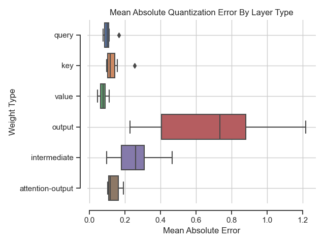
(a) Quantization Error

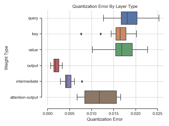
(b) F-Norm Elementwise Errors

Figure 2: Dynamic Quantization of InfoXLM_Base After Quantization Aware Fine-Tuning on XNLI.

Student	Quant Method	Teacher	Quant Method	en	Avg.
XLM-R${}_{\text{Base}}$ Conneau et al.	-	-	-	84.6	74.5
XLM-R${}_{\text{Base}}$	-	-	-	83.9	73.9
InfoXLM${}_{\text{Base}}$	-	-	-	84.1	74.6
InfoXLM${}_{\text{Base}}$	PTQ${}_{\text{Dynamic}}$	-	-	81.7	71.4
XLM-R${}_{\text{Base}}$	PTQ${}_{\text{Dynamic}}$	-	-	80.1	72.5
XLM-R${}_{\text{Base}}$	QNAT	-	-	82.1	70.5
InfoXLM${}_{\text{Base}}$	QNAT	-	-	83.7	73.0
XLM-R${}_{\text{Base}}$	QNAT${}_{\text{KLD}}$	XLM-R${}_{\text{Base}}$	-	83.4	72.5
XLM-R${}_{\text{Base}}$	QNAT${}_{\text{KLD}}$	InfoXLM${}_{\text{Base}}$	-	84.4	73.3
InfoXLM${}_{\text{Base}}$	QNAT${}_{\text{KLD}}$	InfoXLM${}_{\text{Base}}$	-	83.9	73.6
InfoXLM${}_{\text{Base}}$	QNAT${}_{\text{Att}}$	InfoXLM${}_{\text{Base}}$	-	84.1	73.2
InfoXLM${}_{\text{Base}}$	QNAT${}_{\text{Att-KLD}}$	InfoXLM${}_{\text{Base}}$	-	84.1	73.8
InfoXLM${}_{\text{Base}}$	QNAT${}_{\text{Att}}$	InfoXLM${}_{\text{Base}}$	QNAT-PTQ	83.3	72.1
InfoXLM${}_{\text{Base}}$	QNAT${}_{\text{Hid}}$	InfoXLM${}_{\text{Base}}$	QNAT-PTQ	81.1	70.7
InfoXLM${}_{\text{Base}}$	QNAT${}_{\text{KLD}}$	InfoXLM${}_{\text{Base}}$	QNAT-PTQ	83.7	73.1
InfoXLM${}_{\text{Base}}$	QNAT${}_{\text{Att-KLD}}$	InfoXLM${}_{\text{Base}}$	QNAT-PTQ	83.9	73.4
The best performance obtained are marked in bold.

Table 1: XNLI standard and zero-shot test accuracy using (Fake) Quantization-Aware Training with INT-8 Post-Training (Real) Dynamic Quantization.

4 Empirical Results

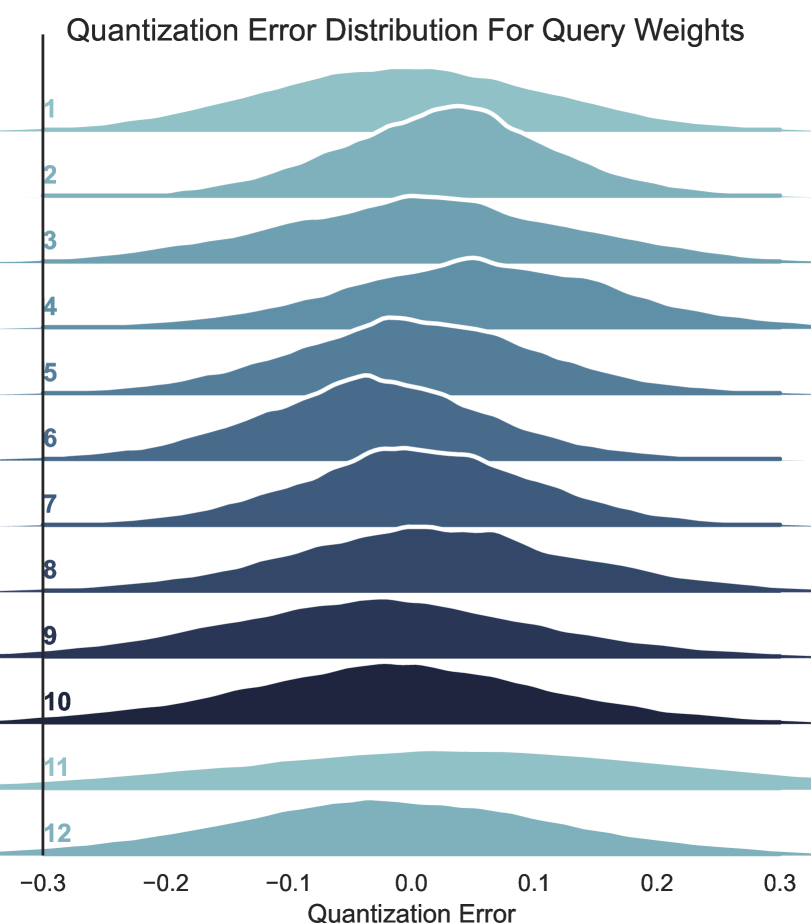
(a) Query

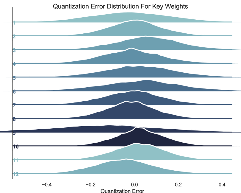
(b) Key

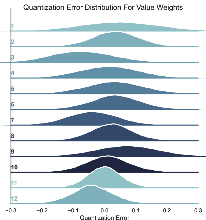
(c) Value

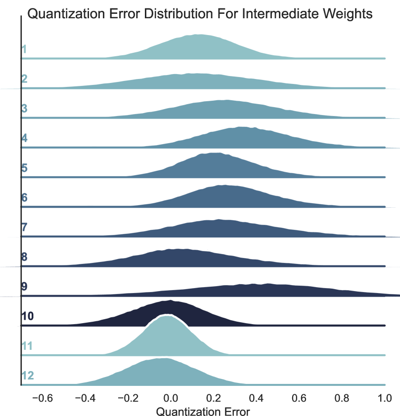
(d) Intermediate Out

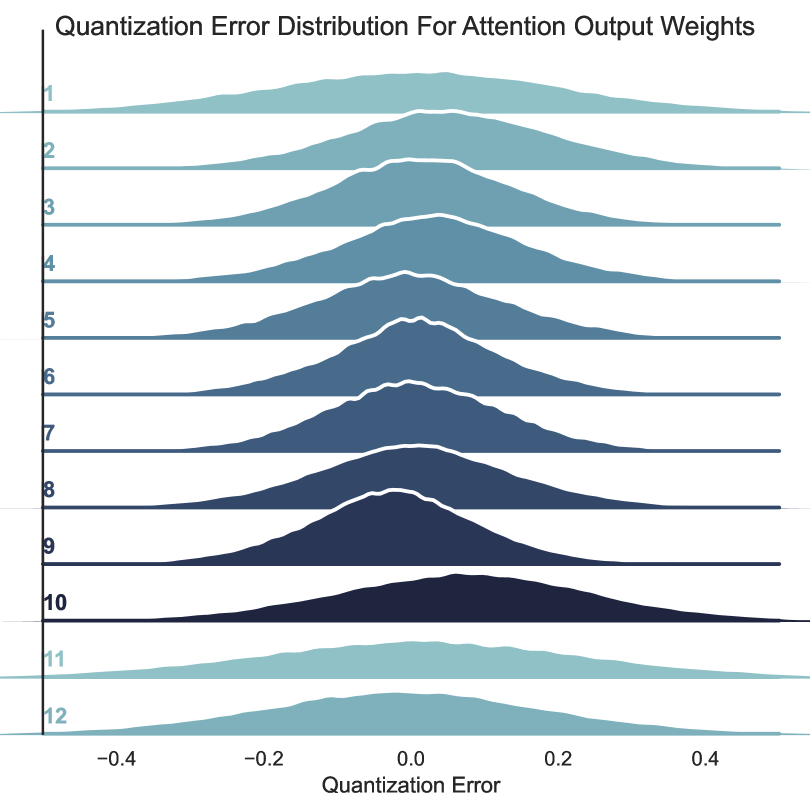
(e) Attention Output

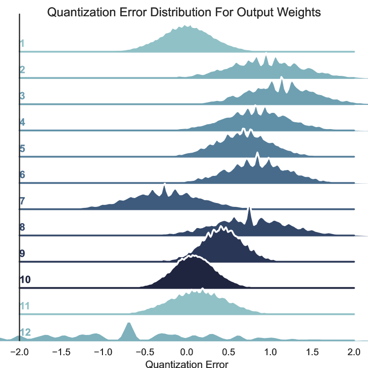
(f) Output

Figure 3: Dynamic Quantization of InfoXLM_Base After Quantization Aware Fine-Tuning on XNLI.

Student	Teacher	Mem	XNLI	NC	NER	PAWSX	POS	QAM	QADSM	WPR	Avg.
X	-	1.22	73.9	83.2	83.8	89.3	79.7	68.4	68.3	73.6	77.5
I	-	1.22	74.6	83.6	85.9	89.6	79.8	68.6	68.9	73.8	78.1
X-PTQ${}_{\text{Dynamic}}$	-	0.52	71.4	81.5	82.9	87.1	76.1	66.3	65.8	68.2	74.9
I-PTQ${}_{\text{Dynamic}}$	-	0.52	72.5	81.8	83.0	87.8	75.8	66.6	66.1	68.7	75.3
X-QNAT	-	0.52	70.5	81.8	83.0	87.4	78.4	66.8	66.9	70.4	75.7
I-QNAT	-	0.52	73.0	82.1	83.1	87.8	78.0	67.2	67.2	70.8	76.2
X-QNAT${}_{\text{KLD}}$	X	0.52	72.5	82.0	83.2	88.1	78.8	67.1	67.2	70.7	75.8
X-QNAT${}_{\text{KLD}}$	I	0.52	73.3	82.1	82.8	88.2	78.3	67.3	67.5	70.5	75.9
I-QNAT${}_{\text{KLD}}$	I	0.52	73.6	82.6	83.1	88.4	79.5	67.6	67.9	71.8	76.8
I-QNAT${}_{\text{Att}}$	I	0.52	73.2	82.4	83.0	88.3	78.3	67.8	67.7	71.7	76.6
I-QNAT${}_{\text{Att-KLD}}$	I	0.52	73.8	82.8	83.4	88.8	79.5	67.9	68.0	72.4	$\underline{\textbf{77.1}}$
I-QNAT${}_{\text{Att}}$	I${}_{\text{QNAT-PTQ}}$	0.52	72.1	82.1	83.1	89.2	78.8	68.0	67.8	71.9	76.6
I-QNAT${}_{\text{Hid}}$	I${}_{\text{QNAT-PTQ}}$	0.52	70.7	81.9	82.4	88.8	78.4	67.3	68.0	71.4	76.1
I-QNAT${}_{\text{KLD}}$	I${}_{\text{QNAT-PTQ}}$	0.52	73.1	82.3	83.0	88.4	79.2	67.6	67.9	72.1	76.7
I-QNAT${}_{\text{Att-KLD}}$	I${}_{\text{QNAT-PTQ}}$	0.52	73.4	82.5	83.3	88.9	79.6	67.9	68.2	72.6	$\underline{\mathbf{77.1}}$

Table 2: XGLUE INT-8 Zero-Shot Quantization Results with Post-Training Dynamic Quantization.

We begin by referring the reader to the supplementary material for the experimental setup in subsection A.2 and  subsection A.3. Before discussing the main results on XGLUE, we first analyse the mean absolute quantization error and the Frobenius norm of the elementwise difference in self-attention blocks between an INT-8 dynamically quantized InfoXLM${}_{\text{Base}}$ and an unquantized FP-32 InfoXLM${}_{\text{Base}}$ in Figure 2. We see in 2(a) that the output layer contains the largest mean absolute error across each layer and highest error variance. In contrast, query, key, value (QKV) parameters have much smaller error. However, since most of the parameters are found in the QKV layers, the sum of the quantization error is larger, as seen in 2(b). This motivates us to focus on the output of the self-attention block when minimizing quantization errors with our proposed loss in Equation 2 as the mean error is higher near the output as it accumulates errors from previous layers in the block. This is also reflected in the parameter distribution of each layer type across all layers in Figure 3, where the x-axis is the mean absolute quantization error and the y-axis is the layer indices. We see the quantization noise is more apparent on the output layer as the Gaussian distrbutions are non-smooth and have clear jitter effect.

XNLI Per Language Results

Table 1 shows the baselines and our SDQ methods applied to XLM-R${}_{\text{Base}}$ and InfoXLM${}_{\text{Base}}$. Here, both models are only trained on the English language and hence the remaining languages in the evaluation set test the zero-shot performance after INT8 quantization (apart from the first 3 rows that show FP-32 fine-tuned results). On average, we find that best student networks results are found when distilling using QNAT${}_{\text{Att-KLD}}$ SDQ with the outputs of an FP-32 teacher for InfoXLM${}_{\text{Base}}$ at 73.8% test accuracy points, where the original FP-32 InfoXLM${}_{\text{Base}}$ achieves 74.6%. Additionally we see that QNAT${}_{\text{Att-KLD}}$ improves over QNAT${}_{\text{KLD}}$ distillation, indicating that attention output distillation improves the generalization of the INT-8 student model. We also found that largest performance drops correspond to languages that less pretraining data and morphologically rich (Swahili, Urdu, Arabic), while performance in English for the best INT-8 XLM-R${}_{\text{Base}}$ (84.4%) is within 0.2% of the original network (84.6%) and the best InfoXLM${}_{\text{Base}}$ that uses QNAT${}_{\text{Att-KLD}}$ is on par with the FP-32 results.

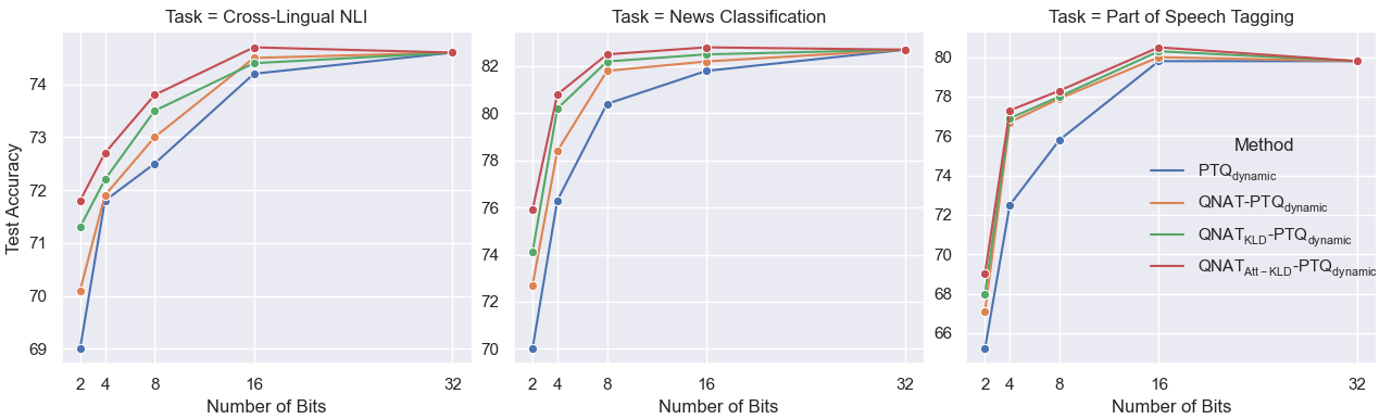
Figure 4: Accuracy versus Number of Bits for XGLUE Tasks with FP-32-16 and INT-8-4-2 formats.

Quantization Results on XGLUE.

We show the per task test performance and the understanding score (i.e average score) on XGLUE for quantization baselines and our proposed SDQ approaches in Table 2 (for brevity we denote InfoXLM${}_{\text{Base}}$ as I and XLM-R${}_{\text{Base}}$). Our proposed QNAT${}_{\text{Att-KLD}}$ achieves the best average (Avg.) score and per task performance for all tasks, using a fine-tuned InfoXLM${}_{\text{Base}}$ (XNLI, NC, NER and QAM) and a fine-tuned InfoXLM${}_{\text{Base}}$ trained with QuantNoise and dynamically quantized post-training (PAWSX, POS, QAM, QADSM and WPR). We also find that QNAT${}_{\text{Att-KLD}}$ improves over QNAT${}_{\text{KLD}}$, highlighting that the attention loss is improving quantized model performance.

Performance versus Compression Rate

Figure 4 shows how the performance changes for four approaches, including two of our proposed objectives (QNAT${}_{\text{KLD}}$ and QNAT${}_{\text{Att-KLD}}$), when training InfoXLM${}_{\text{Base}}$. As before, PTQ${}_{\text{dynamic}}$ is a dynamically quantization fine-tuned InfoXLM${}_{\text{Base}}$ and QNAT-PTQ${}_{\text{dynamic}}$ is the same as PTQ${}_{\text{dynamic}}$ except fine-tuned also using QuantNoise. Unlike our previous results, here we apply fake quantization at inference to achieve compression lower than INT-8 and be comparable to previous work Fan et al. (2019). We see that performance is generally well maintained up until 8 bits. However, performance significantly degrades for all quantization methods for 4 and 2 bit weights. We find that QNAT${}_{\text{Att-KLD}}$ maintains higher performance when compared to the baselines and directly quantizing with no QAT (PTQ${}_{\text{dynamic}}$) leads to the poorest results, also reflected in  Table 2 results with real dynamic quantization at inference time.

Student	Teacher	XNLI	NC	NER	POS	Avg.
-	-	74.6	83.6	85.9	79.7	81.0
iPQ${}_{\text{Scalar}}$	-	69.1	79.4	81.9	76.3	76.7
iPQ${}_{\text{Scalar-KLD}}$	Standard	70.4	80.1	82.3	76.9	77.4
iPQ${}_{\text{Scalar-KLD}}$	iPQ${}_{\text{Scalar}}$	70.8	80.7	82.6	79.4	78.4
iPQ${}_{\text{Scalar-Att-KLD}}$	Standard	72.2	80.4	82.5	77.4	78.1
iPQ${}_{\text{Scalar-Att-KLD}}$	iPQ${}_{\text{Scalar}}$	71.3	80.4	82.9	79.6	78.6
iPQ${}_{\text{EM}}$	-	69.1	79.4	81.9	76.3	76.7
iPQ${}_{\text{EM-KLD}}$	Standard	70.4	80.1	82.3	76.9	77.4
iPQ${}_{\text{EM-KLD}}$	iPQ${}_{\text{EM}}$	72.8	81.6	82.8	79.8	79.3
iPQ${}_{\text{EM-Att-KLD}}$	Standard	73.2	82.3	82.7	79.1	79.3
iPQ${}_{\text{EM-Att-KLD}}$	iPQ${}_{\text{EM}}$	73.1	82.5	83.0	79.2	79.5
QNAT	-	70.5	81.8	83.3	78.4	78.5
QNAT${}_{\text{KLD}}$	Standard	73.2	82.6	83.1	79.5	79.6
QNAT${}_{\text{KLD}}$	QNAT	73.1	82.3	83.0	79.2	79.4
QNAT${}_{\text{Att-KLD}}$	Standard	73.8	82.8	83.4	79.5	79.9
QNAT${}_{\text{Att-KLD}}$	QNAT	73.4	82.5	83.3	79.6	79.7

Table 3: SoTA INT-8 Iterative Product Quantization methods with and without SDQ for InfoXLM${}_{\text{Base}}$.

Ablation with Current QAT Methods

Table 3 shows the results from XGLUE tasks where the first two columns describe how the student and teacher networks are trained and “Standard” refers to standard FP-32 fine-tuning. This includes iPQ Stock et al. (2019) with scalar quantization (iPQ${}_{\text{Scalar}}$), iPQ that uses expectation maximization to create the codebook during training (iPQ${}_{\text{EM}}$) and previous results of QuantNoise (QNAT) as a reference point. In this setup, we only apply the attention loss, $\ell_{\text{Attention}}$, to the layers that are quantized during iPQ. In all cases, adding that SDQ distillation of the classification output and the self-attention outputs improves the average performance.

5 Conclusion

In this paper we proposed an attention-based distillation that minimizes accumulative quantization errors in fine-tuned masked language models. We identified that most of the quantization errors accumulate at the output of self-attention blocks and the parameter distribution of the output layer is effected more by quantization noise. The proposed distillation loss outperforms baseline distillation without the attention loss and the resulting INT-8 models are within 1 understanding score points on the XGLUE benchmark with real quantization post-training. Moreover, fine-tuning the teacher network with quantization-aware training can further improve student network performance on some of the tasks. Further compression can be achieved up to 4-bit and 2-bit weights but performance steeply degrades as the network capacity is drastically reduced coupled with the models having to generalize to multiple languages it was not trained on.

6 Limitations

Dataset and Experimental Limitations.

The datasets and tasks we focus on are from the XGLUE benchmark Liang et al. (2020). The structured prediction tasks, namely Named Entity Recognition (NER) and Part of Speech (PoS) Tagging, both have a limited number of training samples at 15k and 25.4k samples respectively. This is due to the difficulty in annotating on the token level, however it can still be viewed as a limitation when compared to the remaining sentence-level tasks the majority of tasks have at least 100k samples.

Methodological Limitations.

Below are a list of the main methodological limitations we perceive of our work:

• Our method requires a teacher model that is already trained on the downstream task which can then be used to perform knowledge distillation. This is limiting when there are constraints on the computing resources required to produce the quantized model.

• We have focused on the problem of reducing accumulative qunatization errors which become more apparent the deeper a network is. However, this problem is intuitvely lessened when the model is shallow (e.g 3-4 layers) but perhaps wider. Hence the results may be less significant if the model is shallower than what we have experimented in this work.

• By introducing the distillation loss we require an additional regualrization term $\beta$ to be optimally set, relative to the main distillation loss $\alpha$. This can be viewed as a potential limitation has it introduced an additional hyperparameter to be searched to obtain best results on a given task.

• Lastly, since intermediate layer outputs of the teacher network are required for self-attention distillation, we have to perform two forward passes during training. Since standard KLD distillation only requires the output logits, it is common to store the training data teacher logits, eliminating the need to perform two forward passes at training data. However, this is not an option with self-atttention outputs as the storage required offline scales with the number of self-attention heads, number of layers and the size of the training data.

7 Ethics Statement

Here we briefly discuss some ethical concerns of using such compressed models in the real world, specifically the two techniques used in this work, quantization and knowledge distillation. Hooker et al. (2020) have found that compressed models can amplify existing algorithmic bias and perform very poorly on a subset of samples while the average out-of-sample accuracy is maintained close to the uncompressed model. This general finding for pruning and quantization may be also extrapolated to our work (including distillation), hence it is important to recognize that our work, much like the remaining literature on compression, may have ethical concerns with regards to algorithmic bias and how that effects downstream tasks. However, smaller models are more cost-efficient and thus become more widely available to the general public. To summarize, it is important to analyse any aforementioned bias amplification for subsets of samples for downstream tasks compressed models are used for.

Appendix A Supplementary Material

A.1 Self-Attention in Transformers

Consider a dataset $D=\{(X_{i},y_{i})\}_{i=1}^{m}$ for $D\in\mathcal{D}$ and a sample $s:=(X,y)$ where the sentence $X:=(x_{1},\ldots x_{n})$ with $n$ being the number of words $x\in X$. We can represent a word as an input embedding $\bm{x}_{w}\in\mathbb{R}^{d}$, which has a corresponding target vector $\bm{y}$. In the pre-trained transformer models we use, $X_{i}$ is represented by 3 types of embeddings; word embeddings ($\text{\bf X}_{w}\in\mathbb{R}^{n\times d}$), segment embeddings ($\text{\bf X}_{s}\in\mathbb{R}^{n\times d}$) and position embeddings ($\text{\bf X}_{p}\in\mathbb{R}^{n\times d}$), where $d$ is the dimensionality of each embedding matrix. The self-attention block in a transformer mainly consists of three sets of parameters: the query parameters $\text{\bf Q}\in\mathbb{R}^{d\times l}$, the key parameters $\text{\bf K}\in\mathbb{R}^{d\times l}$ and the value parameters $\text{\bf V}\in\mathbb{R}^{d\times o}$. For 12 attention heads (as in XLM-R${}_{\text{Base}}$ and InfoXLM${}_{\text{Base}}$), we express the forward pass as follows:

$$\overrightarrow{\text{\bf X}}=\text{\bf X}_{w}+\text{\bf X}_{s}+\text{\bf X}_{p}$$ (3)

$$\overrightarrow{\text{\bf Z}}:=\bigoplus_{i=1}^{12}\text{softmax}\big{(}\overrightarrow{\text{\bf X}}\text{\bf Q}_{(i)}\text{\bf K}^{T}_{{(i)}}\overrightarrow{\text{\bf X}}^{T}\big{)}\overrightarrow{\text{\bf X}}\text{\bf V}_{(i)}$$ (4)

$$\overrightarrow{\mathbb{Z}}=\text{Feedforward}(\text{LayerNorm}(\overrightarrow{\text{\bf Z}}+\overrightarrow{\text{\bf X}}))$$ (5)

$$\overleftarrow{\mathbb{Z}}=\text{Feedforward}(\text{LayerNorm}(\overleftarrow{\text{\bf Z}}+\overleftarrow{\text{\bf X}}))$$ (6)

The last hidden representations of both directions are then concatenated $\mathbb{Z}^{\prime}:=\overleftarrow{\mathbb{Z}}\bigoplus\overrightarrow{\mathbb{Z}^{\prime}}$ and projected using a final linear layer $\text{\bf W}\in\mathbb{R}^{d}$ followed by a sigmoid function $\sigma(\cdot)$ to produce a probability estimate $\hat{y}$, as shown in (7). Words from (step-3) that are used for filtering the sentences are masked using a [PAD] token to ensure the model does not simply learn to correctly classify some samples based on the association of these tokens with counterfacts. A linear layer is then fine-tuned on top of the hidden state, $\bm{h}_{X,\texttt{[CLS]}}$ emitted corresponding to the [CLS] token. This fine-tunable linear layer is then used to predict whether the sentence is counterfactual or not, as shown in Equation 7, where $\mathcal{B}\subset D$ is a mini-batch and $\mathcal{L}_{ce}$ is the cross-entropy loss.

$$\mathcal{L}_{ce}:=\frac{1}{|\mathcal{B}|}\sum_{(X,y)\in\mathcal{B}}\bm{y}\log\big{(}\sigma(\bm{h}_{X,\texttt{[CLS]}}\cdot\text{\bf W})\big{)}$$ (7)

Configurations We use XLM-R${}_{\text{Base}}$ and InfoXLM${}_{\text{Base}}$, which uses 12 Transformer blocks, 12 self-attention heads with a hidden size of 768. The default size of 512 is used for the sentence length and the sentence representation is taken as the final hidden state of the first [CLS] token.

A.2 Experimental Setup and Hardware Details

Below describes the experimental details, including model, hyperparameter and quantization details. We choose modestly sized cross-lingual language models as the basis of our experiments, namely XLM-R${}_{\text{Base}}$ Conneau et al. (2019) and InfoXLM${}_{\text{Base}}$ Chi et al. (2020), both approximately 1.1GB in memory and these pretrained models are retrieved from the huggingface model hub.

We choose both XLM-R${}_{\text{Base}}$ and InfoXLM${}_{\text{Base}}$ because they are relatively small Transformers and are required to generalized to languages other than the language used for fine-tuning. Hence, we begin from a point that model are already relatively difficult to compress and are further motivated by the findings that larger overparameterized networks suffer less from PTQ to 8-bit integer format and lower (Jacob et al., 2018; Krishnamoorthi, 2018).

For both XLM-R${}_{\text{Base}}$ and InfoXLM${}_{\text{Base}}$ the hyper-parameters are set as follows: 768 hidden units, 12 heads, GELU activation, a dropout rate of 0.1, 512 max input length, 12 layers in encoder. The Adam Optimizer with a linear warm-up Vaswani et al. (2017) and set the learning rate to 2e-5 for most tasks. For all sentence classification tasks the batch size is set to 32 and we fine-tune with 10 epochs. For POS Tagging and NER, we fine-tune with 20 epochs and set the learning rate to 2e-5. We select the model with the best average results on the development sets of all languages. For SDQ-based models, we report the best performing model for $\alpha\in[0.1,0.2,0.5,0.8]$ and $\beta\in[10,100,200,500]$. All experiments are carried out on Tesla V100-SXM2 32 Gigabyte GPUs NVIDIA (2017) with no constraint on GPU hours used on these machines. In all reported results, we report the best (max) result from 8-16 different runs when searching for $\alpha$ and $\beta$ depending on each particular task.

A.3 Model Configuration and Hyperparameter Settings

XLM-R${}_{\text{Base}}$ and InfoXLM${}_{\text{Base}}$ uses 12 Transformer blocks, 12 self-attention heads with a hidden size of 768. The default size of 512 is used for the sentence length and the sentence representation is taken as the final hidden state of the first [CLS] token. A fine-tuned linear layer W is used on top of both models, which is fed to through a softmax function $\sigma$ as $p(c|h)=\sigma(\text{\bf W}\bm{h})$ where $c$ is used to calibrate the class probability estimate and we maximize the log-probability of correctly predicting the ground truth label.

Table 4 shows the pretrained model configurations that were already predefined before our experiments. The number of (Num.) hidden groups here are the number of groups for the hidden layers where parameters in the same group are shared. The intermediate size is the dimensionality of the feed-forward layers of the the Transformer encoder. The ‘Max Position Embeddings’ is the maximum sequence length that the model can deal with.

Hyperparameters	XLM-R${}_{\text{Base}}$	InfoXLM${}_{\text{Base}}$
Vocab Size	250002	250002
Max Pos. Embeddings	514	514
Hidden Size	3072	3072
Encoder Size	768	768
Num. Hidden Layers	12	12
Num. Hidden Groups	1	1
Num. Attention Heads	12	12
Hidden Activations	GeLU	GeLU
Layer Norm. Epsilon	$10^{-12}$	$10^{-12}$
Fully-Connected Dropout Prob.	0.1	0.1
Attention Dropout Prob.	0	0

Table 4: Model Hyperparameter Settings

We now detail the hyperparameter settings for transformer models and the baselines. We note that all hyperparameter settings were performed using a manual search over development data.

A.3.1 Transformer Model Hyperparameters

We did not change the original hyperparameter settings that were used for the original pretraining of each transformer model. The hyperparameter settings for these pretrained models can be found in the class arguments python documentation in each configuration python file in the https://github.com/huggingface/transformers/blob/master/src/transformers/ e.g configuration_.py.For fine-tuning transformer models, we manually tested different combinations of a subset of hyperparameters including the learning rates $\{50^{-4},10^{-5},50^{-5}\}$, batch sizes $\{16,32,128\}$, warmup proportion $\{0,0.1\}$ and $\epsilon$ which is a hyperparameter in the adaptive momentum (adam) optimizer. Please refer to the huggingface documentation at https://github.com/huggingface/transformers for further details on each specific model e.g at https://github.com/huggingface/transformers/blob/master/src/transformers/modeling_roberta.py, and also for the details of the architecture that is used for sentence classification and token classification.

References

- Banner et al. (2018) Ron Banner, Itay Hubara, Elad Hoffer, and Daniel Soudry. 2018. Scalable methods for 8-bit training of neural networks. Advances in neural information processing systems, 31.
- Bondarenko et al. (2021) Yelysei Bondarenko, Markus Nagel, and Tijmen Blankevoort. 2021. Understanding and overcoming the challenges of efficient transformer quantization. arXiv preprint arXiv:2109.12948.
- Chi et al. (2020) Zewen Chi, Li Dong, Furu Wei, Nan Yang, Saksham Singhal, Wenhui Wang, Xia Song, Xian-Ling Mao, Heyan Huang, and Ming Zhou. 2020. Infoxlm: An information-theoretic framework for cross-lingual language model pre-training. arXiv preprint arXiv:2007.07834.
- Chin et al. (2020) Ting-Wu Chin, Pierce I-Jen Chuang, Vikas Chandra, and Diana Marculescu. 2020. One weight bitwidth to rule them all. In European Conference on Computer Vision, pages 85–103. Springer.
- Conneau et al. (2019) Alexis Conneau, Kartikay Khandelwal, Naman Goyal, Vishrav Chaudhary, Guillaume Wenzek, Francisco Guzmán, Edouard Grave, Myle Ott, Luke Zettlemoyer, and Veselin Stoyanov. 2019. Unsupervised cross-lingual representation learning at scale. arXiv preprint arXiv:1911.02116.
- Dettmers et al. (2022) Tim Dettmers, Mike Lewis, Younes Belkada, and Luke Zettlemoyer. 2022. Gpt3. int8 (): 8-bit matrix multiplication for transformers at scale. Advances in Neural Information Processing Systems, 35:30318–30332.
- Faghri et al. (2020) Fartash Faghri, Iman Tabrizian, Ilia Markov, Dan Alistarh, Daniel M Roy, and Ali Ramezani-Kebrya. 2020. Adaptive gradient quantization for data-parallel sgd. Advances in neural information processing systems, 33:3174–3185.
- Fan et al. (2019) Angela Fan, Edouard Grave, and Armand Joulin. 2019. Reducing transformer depth on demand with structured dropout. arXiv preprint arXiv:1909.11556.
- Fan et al. (2020) Angela Fan, Pierre Stock, Benjamin Graham, Edouard Grave, Rémi Gribonval, Herve Jegou, and Armand Joulin. 2020. Training with quantization noise for extreme model compression. arXiv preprint arXiv:2004.07320.
- Hinton et al. (2015) Geoffrey Hinton, Oriol Vinyals, and Jeff Dean. 2015. Distilling the knowledge in a neural network. arXiv preprint arXiv:1503.02531.
- Hooker et al. (2020) Sara Hooker, Nyalleng Moorosi, Gregory Clark, Samy Bengio, and Emily Denton. 2020. Characterising bias in compressed models. arXiv preprint arXiv:2010.03058.
- Jacob et al. (2018) Benoit Jacob, Skirmantas Kligys, Bo Chen, Menglong Zhu, Matthew Tang, Andrew Howard, Hartwig Adam, and Dmitry Kalenichenko. 2018. Quantization and training of neural networks for efficient integer-arithmetic-only inference. In Proceedings of the IEEE conference on computer vision and pattern recognition, pages 2704–2713.
- Kim et al. (2019) Jangho Kim, Yash Bhalgat, Jinwon Lee, Chirag Patel, and Nojun Kwak. 2019. Qkd: Quantization-aware knowledge distillation. arXiv preprint arXiv:1911.12491.
- Kim et al. (2020) Jangho Kim, KiYoon Yoo, and Nojun Kwak. 2020. Position-based scaled gradient for model quantization and sparse training. arXiv preprint arXiv:2005.11035.
- Kim et al. (2021) Sehoon Kim, Amir Gholami, Zhewei Yao, Michael W Mahoney, and Kurt Keutzer. 2021. I-bert: Integer-only bert quantization. In International conference on machine learning, pages 5506–5518. PMLR.
- Krishnamoorthi (2018) Raghuraman Krishnamoorthi. 2018. Quantizing deep convolutional networks for efficient inference: A whitepaper. arXiv preprint arXiv:1806.08342.
- Liang et al. (2020) Yaobo Liang, Nan Duan, Yeyun Gong, Ning Wu, Fenfei Guo, Weizhen Qi, Ming Gong, Linjun Shou, Daxin Jiang, Guihong Cao, et al. 2020. Xglue: A new benchmark datasetfor cross-lingual pre-training, understanding and generation. In Proceedings of the 2020 Conference on Empirical Methods in Natural Language Processing (EMNLP), pages 6008–6018.
- Mishra and Marr (2017) Asit Mishra and Debbie Marr. 2017. Apprentice: Using knowledge distillation techniques to improve low-precision network accuracy. arXiv preprint arXiv:1711.05852.
- Neill (2020) James O’ Neill. 2020. An overview of neural network compression. arXiv preprint arXiv:2006.03669.
- NVIDIA (2017) Tesla NVIDIA. 2017. Nvidia tesla v100 gpu architecture. Tesla NVIDIA.
- Polino et al. (2018) Antonio Polino, Razvan Pascanu, and Dan Alistarh. 2018. Model compression via distillation and quantization. arXiv preprint arXiv:1802.05668.
- Prato et al. (2019) Gabriele Prato, Ella Charlaix, and Mehdi Rezagholizadeh. 2019. Fully quantized transformer for machine translation. arXiv preprint arXiv:1910.10485.
- Stock et al. (2019) Pierre Stock, Armand Joulin, Rémi Gribonval, Benjamin Graham, and Hervé Jégou. 2019. And the bit goes down: Revisiting the quantization of neural networks. arXiv preprint arXiv:1907.05686.
- Vaswani et al. (2017) Ashish Vaswani, Noam Shazeer, Niki Parmar, Jakob Uszkoreit, Llion Jones, Aidan N Gomez, Lukasz Kaiser, and Illia Polosukhin. 2017. Attention is all you need. arXiv preprint arXiv:1706.03762.
- Wang et al. (2018) Naigang Wang, Jungwook Choi, Daniel Brand, Chia-Yu Chen, and Kailash Gopalakrishnan. 2018. Training deep neural networks with 8-bit floating point numbers. Advances in neural information processing systems, 31.
- Zafrir et al. (2019) Ofir Zafrir, Guy Boudoukh, Peter Izsak, and Moshe Wasserblat. 2019. Q8bert: Quantized 8bit bert. In 2019 Fifth Workshop on Energy Efficient Machine Learning and Cognitive Computing-NeurIPS Edition (EMC2-NIPS), pages 36–39. IEEE.
- Zhao et al. (2019) Ritchie Zhao, Yuwei Hu, Jordan Dotzel, Chris De Sa, and Zhiru Zhang. 2019. Improving neural network quantization without retraining using outlier channel splitting. In International conference on machine learning, pages 7543–7552. PMLR.
- Zhou et al. (2017) Aojun Zhou, Anbang Yao, Yiwen Guo, Lin Xu, and Yurong Chen. 2017. Incremental network quantization: Towards lossless cnns with low-precision weights. arXiv preprint arXiv:1702.03044.