FAIRO: Fairness-aware Adaptation in Sequential-Decision Making for Human-in-the-Loop Systems

Abstract.

Achieving fairness in sequential-decision making systems within Human-in-the-Loop (HITL) environments is a critical concern, especially when multiple humans with different behavior and expectations are affected by the same adaptation decisions in the system. This human variability factor adds more complexity since policies deemed fair at one point in time may become discriminatory over time due to variations in human preferences resulting from inter- and intra-human variability. This paper addresses the fairness problem from an equity lens, considering human behavior variability, and the changes in human preferences over time. We propose FAIRO, a novel algorithm for fairness-aware sequential-decision making in HITL adaptation, which incorporates these notions into the decision-making process. In particular, FAIRO decomposes this complex fairness task into adaptive sub-tasks based on individual human preferences through leveraging the Options reinforcement learning framework. We design FAIRO to generalize to three types of HITL application setups that have the shared adaptation decision problem.

Furthermore, we recognize that fairness-aware policies can sometimes conflict with the application’s utility. To address this challenge, we provide a fairness-utility tradeoff in FAIRO, allowing system designers to balance the objectives of fairness and utility based on specific application requirements. Extensive evaluations of FAIRO on the three HITL applications demonstrate its generalizability and effectiveness in promoting fairness while accounting for human variability. On average, FAIRO can improve fairness compared with other methods across all three applications by $35.36\%$.

1. Introduction

The emerging technologies of sensor networks and mobile computing give the promise of monitoring the humans’ states and their interactions with the surroundings and have made it possible to envision the emergence of human-centered design of Internet-of-Things (IoT) applications in various domains. This tight coupling between human behavior and computing enables a radical change in human life (Picard, 2000). By continuously developing a cognition about the environment and the human state and adapting/controlling the environment accordingly, a new paradigm for IoT systems provides the user with a personalized experience, commonly named Human-in-the-Loop (HITL) systems. With the increasing number of HITL IoT applications being controlled by artificial intelligence (AI) algorithms, the algorithmic fairness of such decision-making algorithms has drawn considerable attention in the last few years (Kleinberg et al., 2018; Rambachan et al., 2020; Dwork et al., 2012; Kusner et al., 2017). Nevertheless, the unique nature of HITL IoT opens a new frontier of algorithmic fairness issues that must be carefully addressed before the wide use of such technologies. In particular, the immense challenge in designing the future HITL IoT lies in respecting human rights and human values, ensuring ethics and fairness, and meeting regulatory guidelines, even while safeguarding our environment and natural resources (Annaswamy et al., 2023).

The following summarizes the key distinctions between the existing literature on algorithmic fairness and the nature of Human-in-the-Loop (HITL) systems:

• Fairness in static/singular decision-making vs fairness in dynamic/sequential decision-making: The current literature on algorithmic fairness primarily addresses the unfairness arising from biases in data and algorithms used in static systems, often employing supervised learning methods. A canonical example comes from a tool used by courts in the United States to make pretrial detention and release decisions (COMPAS) (Northpointe, 2015; Angwin et al., [n. d.]). Other applications include loan applications (Mukerjee et al., 2002), employment processes (Cohen et al., 2019), and markets. In contrast, HITL systems are dynamic, where actions taken at one time have consequences for future states and actions. Therefore, ensuring fairness in HITL systems requires considering the impact of decisions over time, leading to a sequential decision-making problem. Neglecting the dynamic feedback and long-term effects in such systems, as commonly done in static decision-making, can result in harm to sub-populations (Creager et al., 2020; Liu et al., 2018; D’Amour et al., 2020).

• Fairness in decisions (or equality) vs fairness in the impact of decisions (or equity): Existing fairness definitions predominantly focus on equality, aiming to eliminate prejudice or favoritism based on individuals’ characteristics. However, insufficient attention has been given to equity, which entails allocating resources to individuals or groups to support their success (Mehrabi et al., 2021). Equity becomes crucial in HITL systems. Hence, a shift from fairness defined in terms of equality to fairness based on equity is essential.

Motivated by these observations, this paper revisits fairness literature and emphasizes the importance of fairness in sequential decision-making from an equity perspective for HITL systems. The main objective is to operationalize equity in the context of sequential decision-making to develop improved adaptation algorithms tailored to HITL applications.

This paper introduces FAIRO, a novel fairness-aware adaptation framework for sequential-decision making designed for HITL systems. The framework specifically tackles the issue of fairness in situations where multiple humans share the same application space and are collectively impacted by adaptation decisions. While usually these decisions aim to optimize overall system performance, they may inadvertently lead to undesired consequences as humans interact with the system or as the system’s physical dynamics evolve.

2. Related Work

2.1. Fairness in decision-making systems

At the heart of HITL systems is achieving the objective of designing scalable, real-time decision-making mechanisms that are aware of the social context, such as the perceived notion of fairness, social welfare, ethics, and social norms (Sztipanovits et al., 2019; Khargonekar and Sampath, 2020). A vast work in the game theory literature studies various notions of fairness between communities by defining incentive markets between competitors to achieve fairness (Ratliff and Fiez, 2020; Ratliff et al., 2018). Fairness-enhancing interventions have been introduced to machine learning to ensure non-discriminatory decisions by the trained models (Friedler et al., 2019; Hashimoto et al., 2018; Chouldechova and Roth, 2018; Kannan et al., 2018; Goel et al., 2018). In particular, the question of fairness in decision-making systems where the agent prefers one action over another (Jabbari et al., 2017; Joseph et al., 2016; Yu et al., 2019; Gillen et al., 2018; Siddique et al., 2020; Shin et al., 2017) becomes more significant in multi-agent systems (Jiang and Lu, 2019; Hughes et al., 2018). However, imposing fairness constraints as a static, singular decision (as standard supervised learning methods do) while ignoring subsequent dynamic feedback or its long-term effect, especially in sequential decision-making systems, can harm sub-populations (Creager et al., 2020; Liu et al., 2018; D’Amour et al., 2020). Recent work investigates the long-term effects of Reinforcement Learning (RL). It shows that modeling the instantaneous effect of control decisions for single-step bias prevention does not guarantee fairness in later downstream decision actions (Kannan et al., 2019; Milli et al., 2019). Unfortunately, all of this work focused on fairness from the lens of equality—where the target is to ensure no favoritism or bias is present in the system—with very little work that focused on fairness from the lens of equity (mostly in singular/static decision making as opposed to sequential decision-making) (Mehrabi et al., 2021). Indeed, achieving fairness in sequential decision-making systems becomes more complex since policies deemed fair at one point may become discriminatory over time due to variations in human preferences resulting from inter- and intra-human factors (Elmalaki et al., 2018b). This paper focuses on answering this question, especially for HITL systems.

2.2. Different notions of group fairness

The notion of “group fairness” is used in the literature to address the fairness problem when multiple humans are affected by the same adaptation model. While there are several definitions and approaches to defining group fairness, it’s important to note that these approaches may have nuanced variations and can be interpreted differently depending on the context and specific application domain. We only summarize two widely used notions of group fairness: (1) equalized odds, which focuses on achieving similar prediction accuracy across different groups while considering binary classification tasks. It ensures that the true positive rate (sensitivity) and true negative rate (specificity) of a predictive model are comparable across different groups (Hardt et al., 2016), and (2) equal opportunity: aims to ensure that the predictive model provides an equal chance of benefiting from positive outcomes for all groups. In particular, equal opportunity requires that the true positive rate for each group should be approximately equal (Hardt et al., 2016). While these two definitions primarily focus on binary classification tasks, this paper will exploit some of their ideas towards sequential decision-making and not specifically for classification tasks.

2.3. Multi-agent RL and hierarchical RL

Reinforcement Learning (RL) has emerged as a widely used approach for monitoring and adapting to human intentions and responses, enabling personalized sequential adaptations in various contexts (Sadigh et al., 2017; Hadfield-Menell et al., 2016; Elmalaki, 2022). To account for individual variability and response times under different autonomous actions approaches like multisample RL and adaptive scaling RL (ADAS-RL) have been proposed (Elmalaki et al., 2018b; Ahadi-Sarkani and Elmalaki, 2021). Amazon has utilized personalized RL to tailor adaptive class schedules based on students’ preferences (Bassen et al., 2020). Moreover, advancements in deep learning coupled with RL have been leveraged to determine the optimal content to present to students based on their cognitive memory models (Reddy et al., 2017). Hierarchical reinforcement learning (HRL) offers a promising solution for addressing complex learning tasks by decomposing them into multiple simpler sub-tasks. This hierarchical structure effectively decomposes long-horizon and intricate tasks into manageable components. The high-level policy is responsible for selecting optimal sub-tasks, considered high-level actions. In contrast, the lower-level policy focuses on solving the sub-tasks using reinforcement learning techniques. This decomposition strategy enables the transformation of a long timescale task into multiple shorter timescale sub-tasks, potentially making individual sub-tasks easier to solve. For instance, the Option-critic Framework introduces an architecture capable of learning higher and lower-level policies without needing prior knowledge of sub-goals (Bacon et al., 2017). HRL has demonstrated superior performance in various domains, including long-horizon games and continuous control problems (Claure et al., 2020; Hoffman et al., 2018) In this paper, we will decompose the fairness problem into sub-tasks over smaller time horizons and exploit the options framework to solve these sub-tasks.

2.4. Paper contribution

The contributions of this paper can be summarized as follows:

• Fairness from the Lens of Equity: We tackle the fairness problem in sequential-decision making systems within HITL environments by addressing the notion of equity.

• FAIRO: We propose FAIRO, a novel algorithm designed for fairness-aware sequential-decision making in HITL adaptation. Our approach leverages the Options RL framework to effectively incorporate fairness considerations into the decision-making process.

• Generalization to Different HITL Application Setups: We extend FAIRO to cater to three types of HITL application setups. These setups involve multiple humans sharing the application space and being impacted by: (1) global numerical adaptation decisions, (2) shared global resources, and (3) shared global categorical adaptation decisions.

• Evaluation on Multiple HITL Applications: We conduct comprehensive evaluations of FAIRO on three different HITL applications to demonstrate its generalizability.

The paper is structured as follows: Section 3 summarizes the Options framework, which serves as the foundation for our proposed approach. Section 4 details how we leverage the Options framework to incorporate fairness considerations into the decision-making process. The subsequent sections of the paper focus on evaluating our proposed approach, FAIRO, in three distinct application domains.

3. Options framework for temporal abstraction

The Markov Decision Process (MDP) framework is widely employed for modeling sequential decision-making. Various methods are utilized to solve MDPs and obtain the optimal Markov decision chain, including dynamic programming and reinforcement learning (RL). RL is particularly used when the transition probabilities within the MDP are unknown. Within the discrete-time finite MDP setting, the standard RL framework can be applied. In particular, an agent engages with an environment that is modeled as an MDP at discrete time steps, denoted as $t=0,1,2,...$. At each time step $t$, the agent observes the current state of the environment, denoted as $s_{t}\in\mathcal{S}$, and selects an action $a_{t}\in\mathcal{A}$ based on this observation. This action leads to a transition to the next state, $s{t+1}$, and yields a reward value, $r_{t}\leftarrow\mathbb{R}$, associated with this transition. By engaging in this interaction, the agent learns a policy $\pi(s,a)$ that guides its decision-making, aiming to select the best action $a$ for each state $s$ to maximize the expected total reward over sequential decision actions.

The options framework was first introduced by Sutton et al.  (Sutton et al., 1999) to generalize primitive actions to include temporally extended courses of lower-level action. In particular, the term options represents a temporal abstraction of the lower-level actions in the MDP. A pictorial figure of options over MDP is shown in Figure 1. An MDP’s state trajectory comprises small, discrete-time transitions, whereas the options enable an MDP to be abstracted and analyzed in larger temporal transitions.

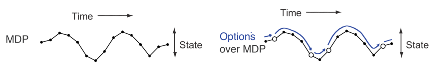
Figure 1. The state trajectory of an MDP with small discrete-time transitions. Options enable overlaid larger abstracted discrete events.

Option $o$ within the option set $\mathcal{O}$ consists of three main components: a policy $\pi(a|s,o)$ for selecting actions within option $o$, an initiation set $\mathcal{I}\subseteq\mathcal{S}$, a termination condition $\beta$. An option $o$:($\mathcal{I},\pi,\beta$) is available to be selected by the agent in state $s_{t}$ if and only if $s_{t}\in\mathcal{I}$. If the option is selected, actions are selected according to the option policy $\pi$ until the option terminates according to the termination condition $\beta$. When the option terminates, the agent can select another option. This definition of options makes them act as much like actions while adding the possibility that they are temporally extended.

The rationale behind employing the options framework to achieve fairness in a multihuman setting stems from the inherent limitations imposed by an option’s initiation set $\mathcal{I}$ and termination condition $\beta$. These constraints confine the applicability of an option’s policy, $\pi$, to a subset defined by $\mathcal{I}$ rather than encompassing the entire state space $\mathcal{S}$. Consequently, options can be viewed as a means of achieving fairness subgoals, wherein each option’s policy is adapted to enhance the attainment of its specific subgoal, thereby contributing to the overall fairness of the decision-making agent. Notably, the dynamic nature of the multihuman environment necessitates the need for diverse fairness policies at different temporal instances. Consequently, in this paper, we leverage the options framework to address fairness concerns within the context of sequential decision-making.

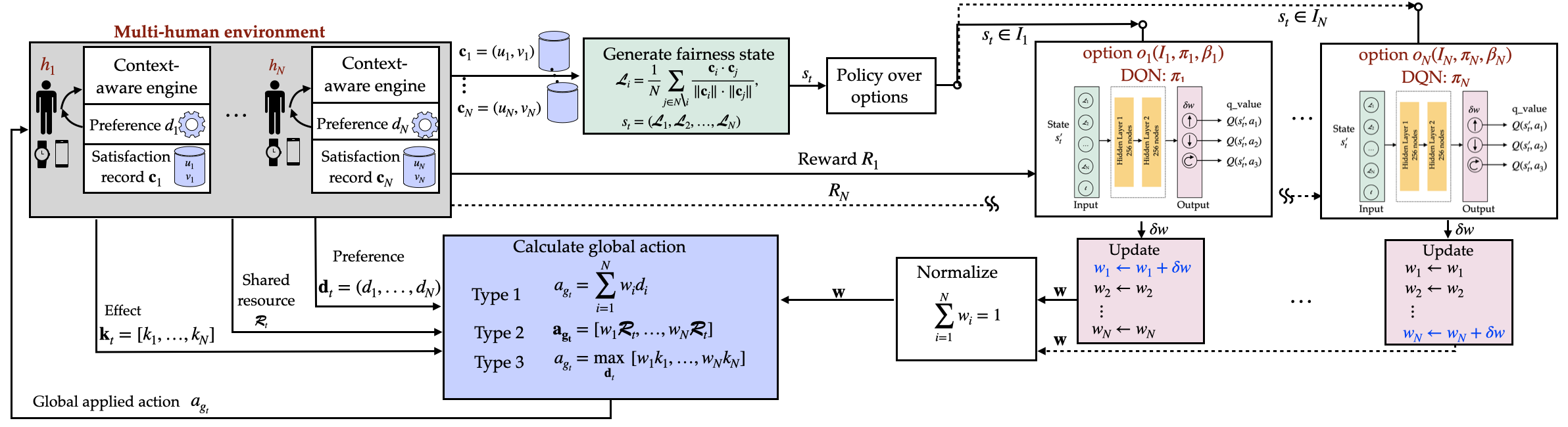
Figure 2. FAIRO for fairness-aware framework in Human-in-the-Loop systems using options framework. FAIRO is designed for three types of applications: Type 1: one global action based on numerical demands affecting multiple humans, Type 2: one shared resource distributed over multiple humans, and Type 3: one global action based on categorical preferences.

4. Fairness using Options framework

We exploit the options framework to design FAIRO to achieve fairness in sequential decision-making agents in multihuman environment. As seen in Figure 2, the agent interacts in sequential discrete-time steps with an environment that has $N$ humans $(h_{1},h_{2},\dots,h_{N})$ through observing their preferences or their desired adaptation actions $(d_{1},d_{2},\dots,d_{N})$ and the current fairness state of the environment $s_{t}$. Guided by the current fairness state $s_{t}$, the agent selects an appropriate option $o_{t}$ from the set of $N$ available options $\mathcal{O}$. The chosen option $o_{t}$ then determines a lower-level action based on its specific option policy $\pi_{o}$, resulting in a global action $a_{g_{t}}$ that is applied to the shared environment. This global action subsequently modifies the current fairness state, and the agent receives a reward $r_{t+1}$. This reward is utilized to refine the option policy. In the following subsections, we provide a detailed description of each module within the FAIRO framework.

4.1. Fairness state space $\mathcal{S}$

Our approach to viewing fairness from the lens of equity is by using a fairness state that encompasses the history of the positive and negative effects of the global decision action.

4.1.1. Satisfaction history records $\mathbf{c}_{i}$

Fairness state $s_{t}$ is inferred from the history of the satisfaction of each human. To model the satisfaction of the human $h_{i}$, we keep a history record for each human:

(1) $$\mathbf{c}_{i}=(u_{i},v_{i}),\text{where }i\in\{1,2,\dots,N\}.$$

The value $u_{i}\in\mathbb{R}$ represents a record of the number of times the human $h_{i}$ was unsatisfied by the applied global action $a_{g}$. In contrast, $v_{i}\in\mathbb{R}$ represents a record for the number of times the human $h_{i}$ was satisfied by the applied global action $a_{g}$.

At time step $t$, every human $h_{i}$ has a desired adaptation action $d_{i_{t}}$. For example, a human may prefer a particular temperature setpoint to HVAC system (Heating, ventilation, and air conditioning) in their room for thermal comfort that matches their physical activities, such as sleeping, domestic work, or sitting (Elmalaki et al., 2018a). Based on the difference in the values of $d_{i_{t}}$ and $a_{g_{t}}$, the record $\mathbf{c}_{i}$ is updated to capture whether the human was satisfied or unsatisfied. For example, if this difference is within a threshold $\tau$ then we consider the human $h_{i}$ is satisfied and increment $v_{i}$ by a value $\delta$.

(2) $$\mathbf{c}_{i}=\begin{cases}(u_{i},v_{i}+\delta)&\|d_{i_{t}}-a_{g_{t}}\|\leq\tau.\\ (u_{i}+\delta,v_{i})&\|d_{i_{t}}-a_{g_{t}}\|>\tau.\end{cases}$$

After all the records $\mathbf{C}=(\mathbf{c}_{i},i=1,2,...,N)$ are updated, they are normalized to a unit vector. Choosing the value $\tau$ is application dependent; however, the value $\delta$ needs to be less than $1$ and small enough to ensure that the unit vector direction $\mathbf{C}$ does not change drastically. Hence, we choose $\delta$ to be $0.01$.

Ideally, these records $\mathbf{c}_{i}$ should be $(0,1)$ indicating that the global adaptation action $a_{g}$ meets the preferences of the human over time. However, as we mentioned earlier, these preferences may conflict with humans sharing the same environment. Hence, the same $a_{g_{t}}$ may be perceived by one human as meeting their preference (increasing $v$) and by another human as not meeting theirs (increasing $u$).

A pictorial visualization of $\mathbf{C}$ is shown in Figure 3. Each $\mathbf{c}_{i}$ can be represented as a $2D$ vector within a unit circle. We show two examples for $\mathbf{c}_{i}$ for three humans where $h_{3}$ has $\mathbf{c}_{3}$ closer to the $v$ axis compared to the other two humans (Figure 3-left) versus the case when $h_{3}$ has $\mathbf{c}_{3}$ closer to the $u$ compared to the other two humans (Figure 3-right). Figure 3 shows an example of a relatively unfair situation, where $h_{3}$ is either treated most of the time favorably (Figure 3-left) or unfavorably (Figure 3-right).

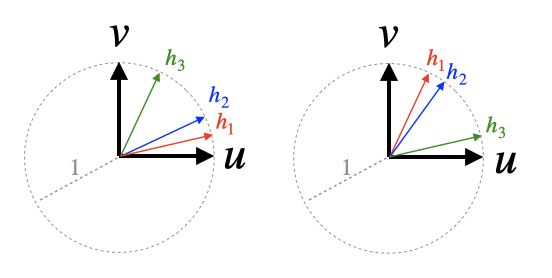
Figure 3. Satisfaction history record $\mathbf{C}$ is represented as $2D$ unit vector, where the two components $v$ and $u$ represent the value that correlates to the number of time steps the human received an adaptation action to the shared environment $a_{g}$ that is close to the preferred desired action $d$ within a threshold $\tau$ or far from it respectively.

It is worth mentioning here that $\mathbf{C}$ captures the history of the effect of the trajectory of sequential adaptation action on the shared environment. Hence, the intuition is to tune the global action in the next time step $a_{g_{t+1}}$ to either decrease the $focus$ on considering the preferences of $h_{3}$ (Figure 3-left) or vice versa (Figure 3-right). However, as mentioned in Section 1, the same action affects all the humans sharing the same environment.

4.1.2. Fairness state $s_{t}$

We use the geometric intuition in Figure 3 to design our fairness state $s_{t}$ to compare the directions of all $N$ records in $\mathbf{C}$. Ideally, we would like to have all $\mathbf{c}_{i}$ as close as possible to each other. Hence, we define $s_{t}$ to capture how close each $\mathbf{c}_{i}$ is to the other $N\text{\textbackslash}i$ records. Hence, we define ($s_{t}$) as follows:

(3) $$\mathcal{L}_{i} =\frac{1}{N}\sum_{j\in N\text{\textbackslash}i}\frac{\mathbf{c}_{i}\cdot\mathbf{c}_{j}}{\|\mathbf{c}_{i}\|\cdot\|\mathbf{c}_{j}\|}, \mathcal{L}_{i}\in]0,1]\subset\mathbb{R}$$

(4) $$s_{t} =(\mathcal{L}_{1},\mathcal{L}_{2},\dots,\mathcal{L}_{N}), s_{t}\in\mathcal{S}=]0,1]^{N}$$

In particular, $\mathcal{L}_{i}$ represents the closeness of record $\mathbf{c}_{i}$ to the rest of the records using the average of the cosine of the angle between pair of vectors. Hence, if the cosine value between two vectors is $1$, they coincide. Since the values of $\mathbf{c}_{i}$ can only be positive and are normalized to a unit vector, the minimum cosine value between these vectors is $0$, indicating that they are far from each other (at $90^{\circ}$). Equation 4 represents $s_{t}$ which holds all the values of $\mathcal{L}_{i}$. Ideally, from our fairness point of view, the goal state $s_{t}$ should be $(1,1,\dots 1)$, which indicates that all $\mathbf{C}_{h}$ have the same direction, meaning that the history of the satisfaction and unsatisfaction for all the humans are close.

4.2. Initiation set $\mathcal{I}$ and fairness subgoals

While the ultimate goal is to learn a policy that can achieve the goal state $s_{t}=(1,1,\dots 1)$, this is challenging since it is a huge state space. Accordingly, the intuition behind exploiting the options framework is to divide this goal into smaller subgoals where we learn over a subset of states or the initiation set ($\mathcal{I}\subseteq\mathcal{S}$) as explained in Section 3. We divide $\mathcal{S}$ into $N$ initiation sets $\mathcal{I}_{i}$ where $i\in\{1,2,\dots,N\}$, such that $\mathcal{I}_{i}$ contains all the states with $\mathcal{L}_{i}$ as the minimum value.

(5) $$\mathcal{I}_{i}=\{s_{t}=\{\mathcal{L}_{1},\ldots,\mathcal{L}_{N}\}\in\mathcal{S}|\mathcal{L}_{i}=\min(s_{t})\}$$

Specifically, this means that each initiation set $\mathcal{I}_{i}$ considers only the states where $h_{i}$ has received unfair adaptation either favorably or unfavorably. For example, both cases in Figure 3 are considered unfair state where $\mathcal{L}_{3}$ is less than $\mathcal{L}_{1}$ and $\mathcal{L}_{2}$.

4.3. Termination State $\beta$

Each option $o_{i}$ terminates when the current state $s_{t}$ reaches a terminal state for this option. Hence, in FAIRO, the set of terminal states for $o_{i}$ is when $\mathcal{L}_{i}$ is no longer the minimum value in $s_{t}$.

(6) $$\beta_{i}=\{s_{t}=\mathcal{L}_{1},\ldots,\mathcal{L}_{N}\}\in\mathcal{S}|\mathcal{L}_{i}\neq\min(s_{t})\}$$

Intuitively, this means that each option $o_{i}$ will run to improve the value of $\mathcal{L}_{i}$ until it is no longer the minimum value which is the fairness subgoal for this option. This will trigger a new initiation set $I$ and this option terminates and a new option starts to achieve another subgoal: improving $\mathcal{L}_{i}$.

4.4. Global action of different HITL applications

As shown in Figure 2, every human ($h_{i}$) has a desired preference ($d_{i}$) for the adaptation action. However, only one action $a_{g}$ is chosen to be applied to the shared environment. In FAIRO, to learn the global action $a_{g}$ that can achieve a better fairness state $s_{t}$ that eventually achieves the fairness subgoal, we categorize the types of applications into three types:

• (Type 1) Shared numerical global action: The desired preferences $d_{i}$ have numerical values and the global action $a_{g}$ is a numerical value. In this case, we design each option to take a weighted sum of these $N$ preferences. These different weights represent the contribution of each human preference $d_{i}$ in the applied global action $a_{g_{t}}$. We will show an instant of this type in a simulated smart home application in Section 5.

  (7) $$\begin{split}a_{g_{t}}&=\sum_{i=1}^{N}w_{i}d_{i},\ \ \ \ w_{i}\in[0,1]\end{split}$$

• (Type 2) Shared global resource: The desired preferences $d_{i}$ have numerical values. There is one resource $\mathcal{R}$ that is shared, time-varying, and it has to be distributed. The global action $\mathbf{a_{g}}_{t}$ is the weighted share of this resource $\mathcal{R}_{t}$ dictated by their desired preferences. We will show an instant of this type in a simulated water distribution application in Section 6.

  (8) $$\begin{split}\mathbf{a_{g}}_{t}&=[w_{1}\mathcal{R}_{t},w_{2}\mathcal{R}_{t},\dots,w_{N}\mathcal{R}_{t}],\ \ \ \ w_{i}\in[0,1]\end{split}$$

• (Type 3) Shared categorical global action: The desired preferences $d_{i}$ have categorical values and the global action $a_{g}$ is one of these categorical values. In this case, the global action selects one of the $d_{i}$ with the maximum weighted effect. In this work, we define the effect of $d_{i}$ as $k_{i}$ to quantify applying $d_{i}$ on all the other $N-i$ humans. This effect can be estimated from the context-aware engine as shown in Figure 2. We will show an instant of this type for smart education application in Section 7.

  (9) $$\begin{split}\mathbf{a_{g}}_{t}&=\max_{d_{i}}[w_{1}k_{1},w_{2}k_{2},\dots,w_{N}k_{N}],\ \ \ \ w_{i}\in[0,1]\end{split}$$

4.5. Learning the option policy ($\pi_{i}$)

Each option policy $\pi_{o}$ learns the appropriate $\mathbf{w}=(w_{1},w_{2},\dots,w_{N})$ for the global action $a_{g_{t}}$ for every state $s_{t}\in\mathcal{I}_{i}$ to reach the termination condition $\beta_{i}$ such that $\sum_{i=1}^{N}w_{i}=1$. These weights are continuous values and learning them for every $s_{t}\in\mathcal{I}_{i}$ is challenging. Hence, we opt for a simpler design of using Deep Q-Network (DQN) to reduce the search space for the appropriate weights as detailed below.

4.5.1. Deep Q-Network (DQN)

DQN is a reinforcement learning algorithm that combines Q-learning with deep neural network (Mnih et al., 2013). In particular, DQN is used with Markov Decision Process (MDP) to learn the best action to apply at a particular state. DQN estimates the action-value function, denoted as $Q(s,a)$, which represents the expected return (reward) for taking action $a$ in state $s$. This is typically represented by a neural network, where the inputs are the state $s$ and the outputs are the estimated action values $Q(s,a)$ for each possible action. At each time step $t$, the DQN agent observes the state $s_{t}$ and selects an action $a_{t}$ based on its current estimate of the Q-function $Q(s,a)$. This can be done through an $\varepsilon$-greedy policy, where the action with the maximum estimated value is selected with a probability of $1-\varepsilon$ and a random action is selected with probability $\varepsilon$. The DQN agent then applies the action, observes the next state $s_{t+1}$ and the reward $r_{t+1}$, and updates its estimate of the Q-function using the following update rule (Sutton and Barto, 2018):

(10) $$\begin{split}Q(s_{t},a_{t})\leftarrow&Q(s_{t},a_{t})+\alpha(r_{t+1}+\gamma\max_{a}Q(s_{t+1},a)-Q(s_{t},a_{t})),\end{split}$$

where $\alpha$ is the learning rate, $\gamma$ is the discount factor, and $\max_{a}Q(s_{t+1},a)$ is the estimated maximum action-value in the next state $s_{t+1}$. DQN aims to learn a policy that maximizes the cumulative reward over time in a given environment. It combines Q-learning with deep learning, allowing the agent to handle high-dimensional observations and non-linear function approximations. Figure 4 shows a pictorial illustration for the design of the DQN in every option $o_{i}$ in FAIRO.

4.5.2. Input to Option DQN ($s_{t}^{\prime}$)

Every option $o_{i}$ runs a DQN where the input is the $s_{t}$. However, to differentiate between the two cases shown in Figure 3 where both $\mathcal{L}_{3}$ is the minimum value in $s_{t}$, we append to $s_{t}$ the relative location of $\mathbf{c}_{3}$ with respect to the $\mathbf{c}_{1}$ and $\mathbf{c}_{2}$.

(11) $$s_{t}^{\prime}=(s_{t},l),\text{ where }s_{t}\in\mathcal{I}_{i},\quad l=\begin{cases}1,&v_{i}=\max_{v}(s_{t}).\\ 0,&\text{otherwise}.\end{cases}$$

This means that if $\mathcal{L}_{i}$ is the minimum in $s_{t}$, option $o_{i}$ will run since $s_{t}\in\mathcal{I}_{i}$. The input to the DQN in option $o_{i}$ will indicate whether $\mathcal{L}_{i}$ has the minimum value (unfair situation) because $h_{i}$ received favorable treatment relative to all $h_{N\textbackslash i}$ (i.e., $\mathbf{c}_{i}$ has a high $v_{i}$ component) and in this case $l=1$ in Equation 11, or $l=0$ otherwise.

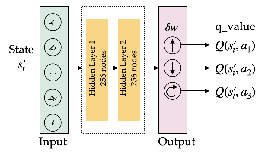
Figure 4. DQN for option $o_{i}$. The input is the state $s_{t}^{\prime}$. The output is the q_value for the possible three actions of weight adjustment $\delta w$.

4.5.3. Output from Option DQN ($\delta w_{i})$

To reduce the action space of the DQN since we need to learn $N$ weights with continuous values $[0,1]$, we designed the output from the DQN in option $o_{i}$ to focus only on adjusting $w_{i}$ instead of all the $N$ weights $\mathbf{w}$. In particular, as shown in Figure 4, the output from the DQN are the Q-values ($Q(s,a)$) which decides to select between three actions to ($a_{1}$) increase the weight $w_{i}$ $\uparrow$, ($a_{2}$) decrease the weight $w_{i}$ $\downarrow$, or ($a_{3}$) keep the same weight $w_{i}$ $\circlearrowright$. Hence, the output from DQN (which is the selected action of the DQN as explained in Section 4.5.1) is the weight adjustment for $w_{i}$ by $\delta w_{i}=(+\delta,-\delta,0)$ where the value $\delta$ determines how fast the DQN for option $o_{i}$ changes the weight $w_{i}$.

(12) $$w_{i}\leftarrow w_{i}+\delta w_{i}$$

Since all the weights $\mathbf{w}$ have to be normalized to $1$, all the weights will be adjusted accordingly. Using this design, we choose between $3$ possible adjustments for weight $w_{i}$ instead of the whole space $[0,1]$ and instead of all the $N$ weights. Accordingly, at every time step $t$, each weight in $\mathbf{w}$ is adjusted due to the normalization.

(13) $$\sum_{i=1}^{N}w_{i}=1,\qquad\mathbf{w}\leftarrow\mathbf{w}+\Delta\mathbf{w}$$

4.5.4. Option DQN reward ($R_{i}$)

Each option DQN learns the appropriate policy $\pi_{i}(s_{t}^{\prime},\delta w_{i})$, which is the right weight adjustment $\delta w_{i}$ at state $s_{t}^{i}$. The DQN learns this policy through a notion of a feedback reward as explained in Section 4.5.1. As each option $o_{i}$ aims at increasing the fairness subgoal of enhancing $\mathcal{L}_{i}$ while improving the performance of the application, the reward function $R_{i}$ can be expressed with two terms; a fairness term $\mathcal{F}$, and a performance term $\mathcal{P}$ using a trade-off parameter $\zeta\in[0,1]$.

(14) $$\begin{split}R_{i}&=\zeta\mathcal{F}_{i}+(1-\zeta)\mathcal{P}_{i},\in[-1,1]\subset\mathbb{R}\\ \mathcal{F}_{i}&=\text{absolute fairness}+\text{option improvement}\\ &=(2*\mathcal{L}_{i_{t}}-1)+f(\mathcal{L}_{i_{t-1}},\mathcal{L}_{i_{t}}),\in[-1,1]\subset\mathbb{R}\\ \mathcal{P}_{i}&=\text{application dependent},\in[-1,1]\subset\mathbb{R}\end{split}$$

In particular, the fairness $\mathcal{F}_{i}$ considers the current value of $\mathcal{L}_{i}$, which we call the “absolute fairness”, and the “improvement in the fairness” value of $\mathcal{L}_{i}$ from last time step for this particular option. It is a function ($f$) of the current value of $\mathcal{L}_{i_{t}}$ and the value from last time step $\mathcal{L}_{i_{t-1}}$ as shown in Equation 14.

The overall FAIRO algorithm is listed in Algorithm 1.

Algorithm 1 FAIRO algorithm

1:

2:Humans $\mathcal{H}=(h_{1},\dots,h_{N})$

3:Satisfaction records $\mathbf{C}=(\mathbf{c_{1}},\dots,\mathbf{c_{N}}),\mathbf{c}_{i}=(u,v)\in\mathbb{R}^{2}$

4:States $s\in\mathcal{S}=]0,1]^{N}\subset\mathbb{R}^{N}$

5:Initiation sets $\mathcal{I}_{i}\in\mathcal{I}=\{s\in\mathcal{S}\}$

6:Options $\mathcal{O}=(o_{1},\dots,o_{N}),o_{i}=(\mathcal{I}_{i},\pi_{i},\beta_{i})$

7:Application type $T=\{Type1,Type2,Type3\}$

8:procedure Run-FAIRO

9:    while True do

10:         $\mathbf{d}_{t}\leftarrow$ context-aware-engine ($\mathcal{H}$)

11:         if $T==Type2$ then

12:             $\mathcal{R}_{t}\leftarrow$ get-current-available-resource()          

13:         if $T==Type3$ then

14:             $\mathbf{k}_{t}\leftarrow$ get-current-effects($\mathbf{d}_{t}$)          

15:         $s_{t}\leftarrow$ get-fairness-state($\mathbf{C}$)

16:         $s_{t}^{\prime}\leftarrow$ append-state($s_{t}$)

17:         $o_{t}\leftarrow$ choose-option ($s_{t}$) $\triangleright$ $o_{t}\in\mathcal{O}$

18:         $\delta w\leftarrow$ run-option($o_{t}$) $\triangleright$ Get the weight adjustments

19:$\triangleright$ based on option policy $\pi_{o}(s_{t},\delta w)$

20:         $\mathbf{w}_{t}\leftarrow$ update-normalize-weights($\delta w$)

21:         $a_{g_{t}}\leftarrow$ calculate-global-action($\mathbf{d}_{t}$, $\mathbf{w}_{t}$,$\mathcal{R}_{t}$, $\mathbf{k}_{t}$ )

22:         $\triangleright$ Apply global action $a_{g_{t}}$ on the shared environment

23:         $R_{t}\leftarrow$ receive-reward ()

24:         $\pi_{o}(s_{t},\delta w)\leftarrow$ Update-option-policy ($R_{t}$)

25:         $\mathbf{C}\leftarrow$ Update satisfaction records ($\mathbf{d}_{t},a_{g_{t}}$)     

5. Application Type 1: Smart Home HVAC

Recent literature focuses on enhancing human satisfaction in smart heating, ventilation, and air conditioning (HVAC) systems by employing reinforcement learning (RL) techniques to adjust the set-point based on human activity and preferences (Jung and Jazizadeh, 2017; Elmalaki, 2021). These HITL systems consider the current state and individual preferences, such as body temperature changes during sleep or physical activity. To evaluate FAIRO in Type 1 applications, we consider a setup where multiple humans share a house with a single HVAC system, and their activities determine individual set-point preferences.

Figure 5. Human 1 activity pattern.

Figure 6. Human 2 activity pattern.

Figure 7. Human 3 activity pattern.

5.1. House-Human Model

We used a thermodynamic model of a house incorporating the house’s shape and insulation type. To regulate indoor temperature, a heater and a cooler with specific flow temperatures ($50^{\circ}c$ and $10^{\circ}c$) were employed. A thermostat maintained the indoor temperature within $2.5^{\circ}c$ around the desired set point. An external controller controls the setpoint. The human was modeled as a heat source, with heat flow dependent on the average exhale breath temperature ($EBT$) and the respiratory minute volume ($RMV$). These parameters depend on human activity (Carroll, 2007). We simulated three humans with four activities: sleeping, relaxing, medium domestic work, and working from home. The different activity schedules depicted in Figures 5, 6, and 7. The humans were simulated in separate rooms, each exhibiting unique behavioral patterns: (1) $h_{1}$ followed an organized and repetitive weekly routine, (2) $h_{3}$ had a more random and unpredictable life pattern, and (3) $h_{2}$ displayed intermediate randomness, alternating between sleeping, being away from home, domestic activities, and relaxation. The Mathworks thermal house model was extended to include a cooling system and a human model.

5.2. Context-aware engine

In Figure 2, a context-aware engine estimates the desired action $d_{i}$ per human $h_{i}$ in a smart home. The desired action can be obtained through fixed policy configuration or learned policy. To focus on our main contribution and not on designing a new context-aware engine, we leverage existing RL-based approaches (Taherisadr et al., 2023) for estimating the desired HVAC setpoint $d_{i}$ based on activity and thermal comfort. The desired setpoints for the considered activities are domestic activity ($72^{\circ}$F), relaxed activity ($77^{\circ}$F), sleeping ($62^{\circ}$F), and work from home ($67^{\circ}$F). These setpoints aim to enhance thermal comfort. Thermal comfort is assessed using Prediction Mean Vote (PMV) on a scale from very cold ($-3$) to very hot ($+3$)(Fanger, 1970). Optimal indoor thermal comfort falls within the recommended range of $[-0.5,0.5]$, as per the ISO standard ASHRAE $55$ (ASHRAE/ANSI Standard 55-2010 American Society of Heating, Refrigerating, and Air-Conditioning Engineers, 2010).

5.3. Evaluation

We compare $5$ different approaches to determine the HVAC setpoint:

• FAIRO: The global applied action is $a_{g_{t}}=\sum_{i=1}^{3}w_{i}d_{i}$ (Equation 7). The reward per option $i$ is as explained in Equation 14. We set $\zeta=0.5$. As for the performance term $\mathcal{P}_{i}$ in the reward, we assign a high reward when the $PMV$ falls in the acceptable range $[-0.5,0.5]$. Further, we used the values of the satisfaction counters $\mathbf{c}_{i}=(u_{i},v_{i})$ as an indication of the performance $\mathcal{P}_{i}$ since their values are correlated to the desired temperature $d_{i}$ which maps to the best PMV. The value $\mathcal{P}_{i}$ is then normalized to be $[-1,1]$:

  (15) $$\begin{split}f&(\mathcal{L}_{i_{t-1}},\mathcal{L}_{i_{t}})=sign(\mathcal{L}_{i_{t-1}}-\mathcal{L}_{i_{t}})\times Z\\ Z&=\begin{cases}0&|\mathcal{L}_{i_{t-1}}-\mathcal{L}_{i_{t}}|\in]0,0.001]\\ 0.25&|\mathcal{L}_{i_{t-1}}-\mathcal{L}_{i_{t}}|\in]0.001,0.005]\\ 0.5&|\mathcal{L}_{i_{t-1}}-\mathcal{L}_{i_{t}}|\in]0.005,0.01]\\ 0.75&|{L}_{i_{t-1}}-\mathcal{L}_{i_{t}}|\in]0.01,0.015]\\ 1&|{L}_{i_{t-1}}-\mathcal{L}_{i_{t}}|>0.015\\ \end{cases}\\ \mathcal{P}_{i}&=0.2\frac{v_{i}}{u_{i}+v_{i}}+0.8f(PMV),\in[-1,1]\subset\mathbb{R}\\ \end{split}$$

• Average approach: The setpoint is the mean value of desired setpoints of all rooms. Hence, $a_{g_{t}}=\frac{1}{3}\sum_{i=1}^{3}d_{i}$.

• Equality using Round Robin (RR): The setpoint is selected from one of the desired setpoints of all rooms in a rotation. The intuition of this approach is to check the case where we give every room the same opportunity to use its desired setpoint across time for equality and how this will affect the overall fairness goal. Hence, for 3 humans, $N=3$, and $a_{g_{1}}=d_{1},a_{g_{2}}=d_{2},a_{g_{3}}=d_{3},a_{g_{4}}=d_{1},a_{g_{5}}=d_{2}\dots,$ etc.

• No subgoals using $1$ DQN with $4$ inputs: The setpoint is calculated using a single model of 1 DQN with the same structure as Figure 4. The inputs are the fairness state ($s_{t}=(\mathcal{L}_{1},\mathcal{L}_{2},\mathcal{L}_{3}$) plus one input which is an indicator of the room number with the minimal value of $\mathcal{L}$. The intuition of this approach is to evaluate whether we can achieve the overall fairness goal without the need for subgoals that the options framework provides. In this case, the reward for the single DQN is the average reward value across all rooms:

  (16) $$\begin{split}\mathcal{R}&=0.5\mathcal{F}+0.5\mathcal{P},\ \ \ \ \text{where }N=3\in[-1,1]\subset\mathbb{R}\\ \mathcal{F}&=\frac{1}{N}\sum_{i=1}^{N}\mathcal{L}_{i}^{N}+f(\frac{1}{N}\sum_{i}\mathcal{L}_{i_{t-1}},\frac{1}{N}\sum_{i=1}^{N}\mathcal{L}_{i_{t}}),\\ \mathcal{P}&=0.2\frac{1}{N}\sum_{i=1}^{N}\frac{v_{i}}{u_{i}+v_{i}}+0.8\frac{1}{N}\sum_{i=1}^{N}f(PMV)\end{split}$$

• No subgoals using $1$ DQN with $3$ inputs: The setpoint is calculated using a single model of 1 DQN structured as Figure 4. The inputs are the three values of the fairness state ($s_{t}=(\mathcal{L}_{1},\mathcal{L}_{2},\mathcal{L}_{3})$) without the extra $4^{th}$ input. The reward is the same as Equation 16.

• FaiRIoT (Elmalaki, 2021): The closest to our approach is FaiRIoT which uses hierarchical RL.

To initialize the values of $s_{t}$ and the weights in the respective DQNs, we use the RR in the first $1200$ samples. To compare these methods, we investigated multiple evaluation metrics to evaluate the fairness across these three rooms; 1) the values of the fairness state ($s_{t}=(\mathcal{L}_{1},\mathcal{L}_{2},\mathcal{L}_{3}$), 2) a satisfaction metric, and the 3) PMV.

5.3.1. Fairness state results

As explained in Section 4.1.2, the best fairness state should be $s_{t}=(\mathcal{L}_{1},\mathcal{L}_{2},\mathcal{L}_{3})=(1,1,1)$. To measure $s_{t}$, we need to use the satisfaction history counters by updating them per to Equation 2. In this application, we set the threshold $\tau$ to be $2.5$. Figure 8 shows the fairness states results with $15$k samples equivalent to $62.5$ simulated days. In Figure 8-first row, we plot the values $\mathcal{L}_{1}$ for Room 1(red), $\mathcal{L}_{2}$ for Room 2(blue), and $\mathcal{L}_{3}$ for Room 3(green). FAIRO achieves $s_{t}=(\approx 0.9991,\approx 0.9989,\approx 0.9991)$ after all the $3$ DQN running in the $3$ options converges at $t_{s}\approx 10k$. As for the Average approach $s_{t}$ stays approximately at $(\approx 0.9957,\approx 0.9962,\approx 0.9982)$, and for the RR approach $s_{t}$ stays at ($\approx 0.9963,\approx 0.9932,\approx 0.9924$).

To better get insights on how the different methods compare with respect to the values of $s_{t}$, in every time sample, we report the maximum value of $\mathcal{L}$ in $s_{t}$ (Figure 8-second row) and the minimum value of $\mathcal{L}$ in $s_{t}$ (Figure 8-third row). The value of $\mathcal{L}_{i}$ gives us an indication of how close Room #$i$ is to the other rooms with respect to the satisfaction history records $\mathbf{c}$ as explained in Equation 4.

The results for using only 1 DQN with 3 and 4 inputs are unstable, and both have fluctuations in the fairness state values. This result is expected for 1 DQN since the fairness goal was not divided into sub-goals, unlike what the options framework provided. For space limitation, we only plot the results of 1 DQN with 3 inputs. However, the 1 DQN with 4 inputs had comparable results.

5.3.2. Compare with group fairness definitions

In Section 2, we discussed the related work and highlighted the commonly used metrics for group fairness, namely, equal opportunity and equalized odds. Although these metrics are typically applied to binary classification tasks, we adopt their original definitions to evaluate and compare FAIRO with the other approaches. In the context of group fairness, equal opportunity aims to ensure that individuals from different groups have an equal chance or probability of experiencing positive outcomes or receiving beneficial treatment or resources. Therefore, to assess the performance of FAIRO, we will analyze the results presented in Figure 8 by examining the reported $\max_{\mathcal{L}}s_{t}$ values. Specifically, we will compare the probabilities of different rooms having the highest $\max_{\mathcal{L}}s_{t}$ values. For equal opportunity, these probabilities need to be close, as denoted in Equation 17.

(17) $$p(Room_{i}==\texttt{find}(\max_{\mathcal{L}}\ s_{t}))\approx p(Room_{N\text{\textbackslash}i}==\texttt{find}(\max_{\mathcal{L}}\ s_{t}))\\$$

As observed in Figure 8-second row, these probabilities are $34\%$, $29.4\%$, and $36.6\%$ for Room $\#1,\#2$, and $\#3$ respectively, which are closer in values compared with the other approaches. In particular, using FAIRO, the average absolute difference between the probabilities of equal opportunity across the 3 rooms is reduced by $57.0\%$, $54.8\%$, $25.8\%$, and $35.8\%$ from Average Approach, RR, 1 DQN 4 inputs and 1 DQN 3 inputs respectively. Accordingly, across all the approaches, FAIRO improves the fairness by $43.35\%$ on average.

While equal opportunity focuses on the balance of the positive outcomes between groups, equalized odds focuses on the balance between positive and negative outcomes across different groups. Hence, for the negative outcomes, we can examine the probabilities of different rooms having the $\min\mathcal{L}s_{t}$ values and assess whether they are approximately equal.

(18) $$p(Room_{i}==\texttt{find}(\min_{\mathcal{L}}\ s_{t}))\approx p(Room_{N\text{\textbackslash}i}==\texttt{find}(\min_{\mathcal{L}}\ s_{t}))$$

As observed in Figure 8-third row, these probabilities are $34.5\%,34.9\%$, and $30.7\%$ for Room $\#1,\#2$, and $\#3$ respectively, which are closer in values compared with the other approaches. In particular, using FAIRO the average absolute difference between the probabilities of equalized odds across the 3 rooms is reduced by $47.8\%$, $35.8\%$, $35.5\%$, and $41.3\%$ from Average Approach, RR, 1 DQN 4 inputs, and 1 DQN 3 inputs respectively.

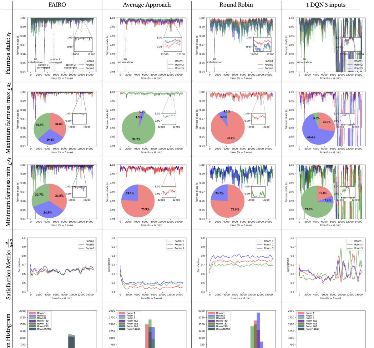
Figure 8. Fairness state and satisfaction metric across all different approaches for application 1.

Histogram	Rooms	FAIRO	Average	RR	1 DQN 4 inputs	1 DQN 3 inputs
Satisfaction Gaussian’s fitting ($\mu,\sigma^{2})$	Room $1$	( 0.642,0.047 )	(0.452,0.030)	(0.748,0.021)	(0.629,0.066)	(0.657,0.142)
	Room $2$	(0.649, 0.050)	(0.506, 0.027)	(0.785,0.023)	(0.628, 0.076)	(0.641,0.084)
	Room $3$	(0.641,0.047)	(0.487,0.030)	(0.698,0.024)	(0.598,0.063)	(0.680,0.152)
Satisfaction JSD	Room $1\&2$	0.022 bits	0.399 bits	0.269 bits	0.015 bits	0.115 bits
	Room $1\&3$	0.002 bits	0.175 bits	0.443 bits	0.049 bits	0.020 bits
	Room $2\&3$	0.014 bits	0.080 bits	0.835 bits	0.041 bits	0.121 bits
	JSD Average	0.013 bits	0.218 bits	0.516 bits	0.035 bits	0.085 bits
PMV Gaussian’s fitting ($\mu,\sigma^{2})$	Room $1$	(0.346,0.490)	(0.369,0.430 )	(0.367, 0.590)	(0.353,0.459)	(0.336,0.502)
	Room $2$	(-0.014,0.612)	(0.021,0.498)	(0.021, 0.701)	(-0.003,0.563)	(-0.030,0.642)
	Room $3$	(-0.099,0.673)	(-0.065,0.564)	(-0.052,0.732)	(-0.095,0.647)	(-0.120,0.723)
PMV JSD	Room $1\&2$	0.088 bits	0.112 bits	0.071 bits	0.092 bits	0.089 bits
	Room $1\&3$	0.119 bits	0.152 bits	0.099 bits	0.124 bits	0.119 bits
	Room $2\&3$	0.012 bits	0.023 bits	0.014 bits	0.014 bits	0.014 bits
	JSD Average	0.073 bits	0.096 bits	0.063 bits	0.077 bits	0.074 bits

Table 1. Comparison of the satisfaction values $\frac{v}{u+v}$ and the PMV across all the approaches in application 1.

5.3.3. Satisfaction performance

In Equation 15, we used $\frac{v}{v+u}$ as one of the performance measures. Figure 8-fourth row shows the satisfaction values for all methods. FAIRO achieves close satisfaction values across the three rooms over time. Average and RR approaches have stable but different satisfaction values across rooms while 1 DQN-3 inputs and 1-DQN-4 inputs show more fluctuations per room. We focused on samples after FAIRO convergence ($12k$ to $15k$) and examined the satisfaction value histograms. Table 1 reports the Jensen-Shannon Divergence (JSD) of these histograms. FAIRO has the lowest average JSD ($0.013$), indicating closer satisfaction values across rooms. The mean value ($\mu$) of the satisfaction histogram fitting into a Gaussian distribution is approximately $0.64$ for all rooms. In particular, compared with other methods, FAIRO JSD is reduced by $94.0\%$ from Average Approach, reduced by $97.5\%$ from RR, reduced by $62.9\%$ from 1 DQN 4 inputs method, and reduced by $84.7\%$ from 1 DQN 3 inputs method. Satisfaction histogram results indicate high similarity in satisfaction across rooms, reflecting fairness in adaptation actions over time. However, FAIRO has a lower mean satisfaction per room compared to the RR, as fairness was an objective in the adaptation. RR has higher values since every time step one of the rooms can have its desired temperature which contributes to the number of samples with $100\%$ satisfaction.

5.3.4. PMV results

We report the statistics of the PMV across all approaches in Table 1. FAIRO achieves the second lowest average JSD and a comparable variance on PMV results, which indicates FAIRO can improve fairness without hurting the PMV performance. The RR can achieve the lowest PMV JSD average since every time step one of the rooms can get exactly its desired temperature. Hence, the $3$ rooms can get almost identical PMV performance in the long term. In summary, FAIRO’s PMV JSD is reduced by $24.0\%$ from Average Approach, increased by $15.9\%$ from RR, reduced by $5.2\%$ from 1 DQN 4 inputs method, and reduced by $1.4\%$ from 1 DQN 3 inputs method.

Figure 9. Coeff. of variation ($cv$) of the temperature differences.

Figure 10. Coeff. of variation ($cv$) of the utility $u_{t}$ over $\mathbf{w}$.

5.3.5. Comparison with the State-of-the-Art FaiRIoT (Elmalaki, 2021)

FaiRIoT uses a notion of utility $u_{h_{t}}=\frac{1}{t}\sum_{j=0}^{t}\frac{j}{t}w_{h_{j}}$ which is the average weight assigned by a layer called “Mediator RL” for a particular human $h$ over a time horizon $[0:t]$, where the factor $\frac{j}{t}$ is used to give more value to the recent weights learnt by the Mediator RL over the ones in the past. FaiRIoT measures the fairness of the Mediator RL using the coefficient of variation ($cv$) of the human utilities: $cv=\sqrt{\frac{1}{n-1}\sum_{h=1}^{n}\frac{(u_{h}-\bar{u})^{2}}{\bar{u}^{2}}},$ where $\bar{u}$ is the average utility of all humans. The Mediator RL is said to be more fair if and only if the $cv$ is smaller. Accordingly, we compare the $cv$ in FaiRIoT and FAIRO in Figure 10. FAIRO achieves $cv$ around $0.15$, while FaiRIoT $cv$ is larger than $0.6$. Hence, FAIRO improves the fairness where cv is reduced by $\mathbf{75\%}$.

6. Type 2: Water supply application

In the context of global climate change and rapid population growth, the planning and management of regional water systems play a crucial role (Council, 2021; wat, 2023). As a result, Water Demand Models (WDMs) have been developed over the past few decades. These models serve two main purposes: gaining insights into water consumption behavior and forecasting demand. WDMs provide valuable inputs for decision-making processes related to the water distribution system (WDS) operation policies and infrastructure planning.

Water authorities and governments have developed multiple management solutions to the water shortage problem  (Jorgensen et al., 2009). However, it is a challenge to allocate water resources if the resource is always limited while providing every household with a fair experience on water resource distribution. Several works in the literature consider pricing and non-pricing policies in water management (Jackson, 2005; Iglesias and Blanco, 2008; Sechi et al., 2013). To evaluate FAIRO for application Type 2, we assume that WDM is available to estimate the desired water demand per three households and the shared water resource to supply these different households is insufficient and time-varying (wat, 2023).

6.1. Household-Water Demand Model

We used a WDM that supplies three households based on their residents’ activity patterns (Avni et al., 2015; Philadelphia Government, 2023). We used the same activity pattern in Section 5.1 and mapped them to water demand behavior as seen in Figure 11 which illustrates the water demand patterns per gallon for three households during three days. Every household has a tank for water reservation $\mathcal{T}$. The desired action for every household $h_{i}$ is to satisfy the water demand $d_{i}$. Water resource ($\mathcal{R}_{t}$) is not fixed and insufficient to satisfy all demands. Since we assume that the WDM is available, we can assume that $\mathcal{R}_{t}$ can follow the demands profiles by choosing it to be $1.5$ the maximum demand of all the three demand profiles. Households’ water demand profiles are independent of each other due to different human activities. We extended the Mathworks Water Supply model to include the household water demand profiles and multiple houses with a limited shared water supply resource (MATLAB, 2023).

6.2. Context-aware engine

To focus on the main contribution and not designing a new water consumption behavior or forecasting demand models, the context-aware engine, as shown in Figure 2 provides the desired action for every household $h_{i}$, which is the current water demand $d_{i}$ based on the water demand pattern. This demand is supposed to be satisfied via the water supply $s_{i}$ from the shared limited resource $\mathcal{R}_{t}$ and the current reserved water in the household water tank $t_{i}$. Hence, we define the application performance as the percentage of balancing the demand and the supply.

(19) $$\text{Balance Rate (BR)}=\frac{\text{supply }s_{i}+\text{reserve }t_{i}}{\text{demand }d_{i}}$$

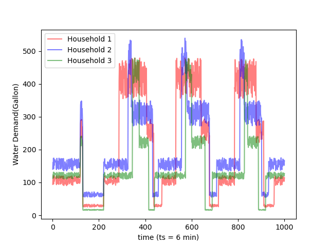
Figure 11. Water demand patterns.

6.3. Evaluation

We compare the same methods as in the first application.

• FAIRO: The supply $s_{i}$ for each household $h_{i}$ is calculated by the FAIRO algorithm. In particular, $s_{i}$ receives $w_{i}\mathcal{R}_{t}$ as explained in Section 4.4 where the global action $a_{g_{t}}$ is the weighted distribution of this resource $\mathcal{R}_{t}$. The reward is the same as explained in the first application in Equation 15 using performance $\mathcal{P}_{i}$ based on the BR. Hence, $\mathcal{P}_{i}=0.2\frac{v_{i}}{u_{i}+v_{i}}+0.8f(\text{BR})$.

• Average approach: Each household $h_{i}$ has the same amount of supply. Hence, $s_{i}=\frac{1}{3}\ \mathcal{R}_{t}$. We further augment the average approach in this application by using a Weighted Average approach. In particular, each household supply is proportional to its demand. Hence, $s_{i}=\frac{d_{i}}{\sum_{i=1}^{3}d_{i}}\mathcal{R}_{t}$.

• Round Robin (RR): Each time step, one of the households in a rotation will be guaranteed sufficient supply to cover its demand. Leftovers from the resource will be shared equally with all households. For example, at time $t=1$, $s_{1}=d_{1}$ while $s_{2}=s_{3}=\frac{\mathcal{R}_{t}-d_{1}}{2}$. We further augmented the RR to consider a Weighted RR. In this case, supplies are calculated similarly to RR, but the leftover water will be distributed proportionally to their demands as in the weighted average approach.

• No subgoals using $1$ DQN with $4$ inputs: Supply for each household is calculated by 1 DQN structure as explained in Section 5.3.

• No subgoals using $1$ DQN with $3$ inputs: Supply for each household is calculated by 1 DQN structure as explained in Section 5.3.

To compare these methods, we investigated multiple evaluation metrics to evaluate the fairness across these three rooms; 1) the fairness state ($s_{t}$) 2) a satisfaction metric, and 3) the balance rate (BR).

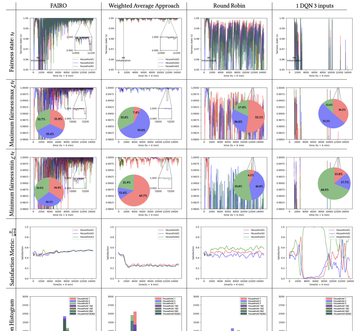
Figure 12. Fairness state and satisfaction metric across all different approaches for application 2.

Histogram	Rooms	FAIRO	Weighted Average	Weighted RR	Average	RR	1 DQN 4 inputs	1 DQN 3 inputs
Satisfaction Gaussian’s fitting ($\mu,\sigma^{2})$	Room $1$	(0.540, 0.037)	(0.267, 0.021)	(0.459, 0.014)	(0.214, 0.100)	(0.496, 0.061)	(0.475, 0.254)	(0.342, 0.280)
	Room $2$	(0.540, 0.029)	(0.249, 0.022)	(0.445, 0.014)	(0.205, 0.085)	(0.462, 0.050)	(0.339, 0.190)	(0.315, 0.257)
	Room $3$	(0.535, 0.048)	(0.244, 0.020)	(0.429, 0.013)	(0.495, 0.105)	(0.596, 0.052)	(0.493, 0.155)	(0.636, 0.241)
Satisfaction JSD	Room $1\&2$	0.016 bits	0.091 bits	0.079 bits	0.088 bits	0.094 bits	0.123 bits	0.048 bits
	Room $1\&3$	0.011 bits	0.150 bits	0.427 bits	0.654 bits	0.390 bits	0.047 bits	0.237 bits
	Room $2\&3$	0.024 bits	0.010 bits	0.165 bits	0.756 bits	0.644 bits	0.135 bits	0.288 bits
	JS Average	0.017 bits	0.084 bits	0.224 bits	0.499 bits	0.376 bits	0.102 bits	0.191 bits
Balance Rate (BR)	avg. ¿80% BR	0.535(1606)	0.254(763)	0.446(1336.7)	0.305(915.3)	0.517(1552)	0.432(1295.7)	0.432(1296.3)

Table 2. Comparison of the satisfaction values $\frac{v}{u+v}$ and the balance rate across all the approaches in application 2.

6.3.1. Fairness state results

We report in Figure  12 the fairness states results with $15k$ samples equivalent to $62.5$ simulated days. To measure $s_{t}$, we need to use the satisfaction history counters by updating them per Equation 2. In this application, we set the $\|d_{i}-(s_{i}+t_{i})\|\leq\tau$ with $\tau$ equals $20\%$ of the demand $d_{i}$ which means BR is $80\%$.

Figure  12-first row plot the fairness state results for each household. FAIRO converges at $t_{s}\approx 10k$. The results of 1 DQN 3 inputs and 1 DQN 4 inputs are unstable with a lot of fluctuations.

6.3.2. Compare with group fairness definitions

Figure 12-second and third rows show the maximum and minimum value of $s_{t}$. FAIRO achieves equal opportunity probabilities $31.9\%$, $35.4\%$, and $32.7\%$ for household $\#1$, $\#2$, and $\#3$ respectively, which are closer in values than other methods. In particular, using FAIRO, the average absolute difference between the probabilities of equal opportunity across the 3 households is reduced by $32.6\%$, $43.5\%$, $27.7\%$, $20.5\%$, $10.6\%$, and $23.4\%$ from Weighted Average, Weighted RR, Average, RR, 1DQN 4 inputs and 1 DQN 3 inputs respectively. Accordingly, across all the approaches, FAIRO improves the fairness by $26.38\%$ on average. As for equalized odds probabilities, FAIRO reports $34.4\%$, $30.1\%$, and $35.5\%$ for households $\#1,\#2$, and $\#3$ respectively, which are also closer in values compared to the other approaches. In particular, using FAIRO, the average absolute difference between the probabilities of equalized odds across the 3 households is reduced by $31.9\%$, $31.0\%$, $37.1\%$, $27.6\%$, $9.4\%$, and $32.9\%$ from Weighted Average, Weighted RR, Average, RR, 1DQN 4 inputs and 1 DQN 3 inputs respectively.

6.3.3. Satisfaction performance

As explained in Equation  15, the value $\frac{v}{v+u}$ is used as a term to measure the performance. Figure  12-forth row reports the satisfaction values across the three households. Satisfaction values in FAIRO are closer compared with other approaches with satisfaction values around $0.55$. RR satisfaction values are from $0.6$ to $0.4$ with different between households. The Weighted Average Approach satisfaction values are close, but values stay below $0.3$. 1 DQN-3 inputs and 1 DQN-4 inputs have unstable fluctuations across $3$ households.

We use $3k$ samples after FAIRO convergence($12k$ to $15k$) to examine the satisfaction value histograms. Table 2 reports the Jensen-Shannon Divergence (JSD) of these histograms. FAIRO has the lowest average JSD ($0.017$), indicating closer satisfaction values across rooms. In particular, compared with other methods, FAIRO JSD is reduced by $79.8\%$, $92.4\%$, $96.5\%$, $95.5\%$, $83.3\%$, and $91.1\%$ from Weighted Average Approach, Weighted RR, Average Approach, RR, 1 DQN 4 inputs, and 1 DQN 3 inputs methods respectively.

6.3.4. Balance rate (BR) results

We report the average number of samples that have $>80\%$ BR across all households in brackets in Table 2 and average it over 3k samples. Samples have $>80\%$ BR correspond to satisfactory samples. Table 2-last row shows FAIRO has the highest average $>80\%$ BR value(0.535). In particular, compared with other methods, FAIRO’s average $>80\%$ BR is improved by $110.6\%$, $20.0\%$, $75.4\%$, $3.5\%$, $23.8\%$, and $23.8\%$ from Weighted Average Approach, Weighted RR, Average Approach, RR, 1 DQN 4 inputs, and 1 DQN 3 inputs methods respectively.

7. Type 3: Smart learning system

Monitoring the human learning state and performance is crucial for assessing progress, identifying gaps, and personalizing instruction (Terai et al., 2020). With the wide adoption of immersive technology, such as virtual reality (VR) in education environments, recent studies showed that these technologies would have a significant impact on the learning (Ibáñez et al., 2014), and workforce training (Irizarry et al., 2013). However, during elongated education periods, especially in an online or VR setup, human performance is prone to significantly decline (Terai et al., 2020) due to distractions, drowsiness, and fatigue. In this application, we examine a setup where multiple humans share the same educational environment, and a HITL learning system adapts this environment by enabling an immersive VR experience to improve the learning experience.

7.1. Human-Learning VR model

We used the dataset associated with recent work in the literature that examined the effect of using VR on the learning performance of $15$ participants watching lectures from Khan Academy (Taherisadr et al., 2023; Academy, 2023). In particular, the human learning experience can be determined through three main features, including alertness level, fatigue level, and vertigo level (Brunnström et al., 2020), forming a total of $8$ states if we use binary values (e.g., Alert:1, Not alert:0) for these features. Indeed different humans may transition between these states based on their experience and preference for VR technology. A HITL learning environment monitors these states and provides the best adaptation action to provide a better learning experience regarding the human state. These adaptation actions can (1) $a_{1}$ give the human a small break, (2) $a_{2}$ enable the use of VR, or (3) $a_{3}$ disable VR. Accordingly, we used this dataset to categorize the $15$ human behavior into three groups. The first group profile has humans who are most tolerant to VR, meaning they do not experience simulator sickness after using VR devices for more than $20$ minutes, the second group profile has humans who can show some cybersickness during VR exposure, and the third group profile has the humans with the least VR tolerance. We model these groups’ behavior using MDP as shown in Figure 13. In particular, state $8$ encodes the best human state regarding high alertness, vigor, and no sense of vertigo or dizziness. In contrast, state $1$ encodes the worst human state. Based on these three human models, we instantiated three humans, one from each profile to run a synthesized experiment of three humans having a class schedule every day. At the beginning of every day, the states of the three humans are initialized to state 3 or state 1 randomly.

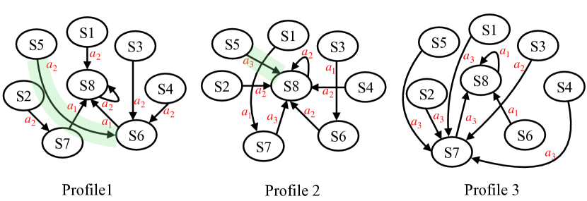
Figure 13. MDP for three human profiles in VR learning environment.

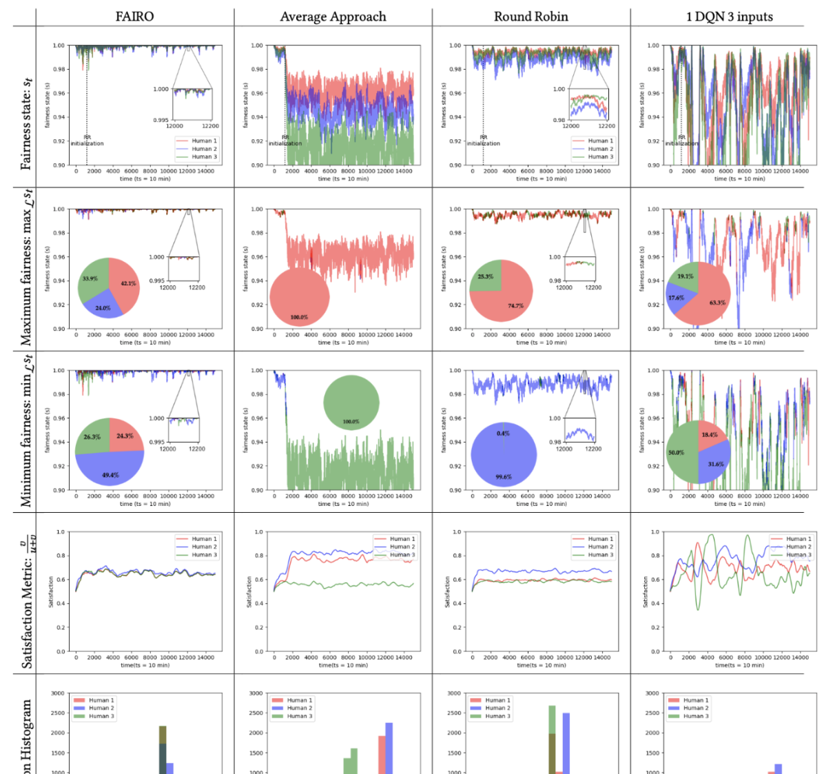
Figure 14. Fairness state and satisfaction metric across all different approaches for application 3.

Histogram	Rooms	FAIRO	Average	RR	1 DQN 4 inputs	1 DQN 3 inputs
Satisfaction Gaussian’s fitting $(\mu,\sigma^{2})$	Room $1$	(0.639, 0.017)	(0.761, 0.033)	(0.594, 0.015)	(0.708, 0.053)	(0.692, 0.062)
	Room $2$	(0.647, 0.020)	(0.821, 0.020)	(0.671, 0.018)	(0.811, 0.057)	(0.787, 0.050)
	Room $3$	(0.638, 0.018)	(0.554, 0.020)	(0.583, 0.012)	(0.638, 0.115)	(0.604, 0.094)
Satisfaction JSD	Room $1\&2$	0.022 bits	0.528 bits	0.801 bits	0.459 bits	0.396 bits
	Room $1\&3$	0.000 bits	1 bits	0.060 bits	0.494 bits	0.229 bits
	Room $2\&3$	0.021 bits	1 bits	0.884 bits	0.538 bits	0.657 bits
	JS Average	0.094 bits	0.843 bits	0.582 bits	0.497 bits	0.427 bits
Learning Experience (LE)	Overlap Samples %	0.488	0.438	0.507	0.473	0.497

Table 3. Comparison of the satisfaction values $\frac{v}{u+v}$ and the learning experience (LE) in application 3.

7.2. Context-aware engine

The desired action $d_{i}$ is selected to improve the human learning experience. Unlike the previous two applications, this application has a non-numerical action space, as mentioned in Section 7.1. Hence, to use FAIRO we need to quantify this categorical action in terms of its effect as explained in Section 4.4. We exploit the MDP model in Figure 13 to quantify these actions. In particular, as $S_{8}$ and $S_{0}$ encode the best and the worst state, respectively, we assign a value to each state linearly with $S_{8}$ as the highest value. Hence, the desired action $d_{i}$ that can make a transition to a better state in the MDP has a high numerical value. However, every human may be in a different state. Hence, for every desired action $d_{i}$, we calculate the effect denoted as $k_{i}$ of applying $d_{i}$ on the other humans. In particular, using the MDP models, if the desired action $d_{i}$ from human $h_{i}$ were to be applied in the shared environment, we check the state transition it will cause on all the other humans $h_{N\text{\textbackslash}i}$. The difference in the values of the two states that $d_{i}$ can cause the transition is used to measure its effect. In our setup, we have three humans; hence to measure the effect $k_{1}$ of applying desired action $d_{1}$ from the first human is the added values of the transition it can cause on human 2 and human 3 based on their current states and their MDP model. Hence, after applying an adaptation action, the human learning experience can be measured as the improvement in the human state values and the current human state value.

(20) $$\text{Learning Experience (LE)}=\text{state improvement}+\text{state value}\ \in[-1,1]$$

7.3. Evaluation

We compare $5$ methods as in the first application.

• FAIRO: The global action $a_{g_{t}}=d_{i}$ is the desired action of the human_i with the maximum weighted effect as explained in Section 4.4. The reward is the same as explained in the first application in Equation 15 using performance $\mathcal{P}_{i}$ based on the learning experience (LE). Hence, $\mathcal{P}_{i}=0.2\frac{v_{i}}{u_{i}+v_{i}}+0.8f(\text{LE})$.

• Average approach: The global action $a_{g_{t}}=d_{i}$ is the desired action of the human_i with the median weighted effect.

• Round Robin (RR): The global action $a_{g_{t}}$ is selected from one of the desired actions of all humans in a rotation.

• No subgoals using 1 DQN with 3 inputs and 1 DQN 4 inputs: The weighted effects are determined by using 1 DQN structure (as explained in Section  5.3) and then the global action is the desired action with the maximum weighted effect.

To compare these methods, we investigated multiple evaluation metrics; 1) the values of the fairness state, 2) a satisfaction metric, and 3) learning experience (LE).

7.3.1. Fairness state results

Figure  14 reports the fairness states results with $15k$ samples. To measure $s_{t}$, we need to use the satisfaction history counters by updating them per Equation 2. In this application, if the learning experience (LE) of the human is $>0$ as measured in Equation 20, it will be considered satisfied. Figure  14-first row plots the fairness state results for 3 humans. FAIRO converges at $t_{s}\approx 10k$.

7.3.2. Compare with group fairness definitions

Figure 12-second and third rows show the maximum and minimum value of $s_{t}$. FAIRO achieves equal opportunity probabilities $42.1\%$, $24.0\%$, and $33.9\%$ for human $\#1$, $\#2$, and $\#3$ respectively. As for equalized odds probabilities, FAIRO reports $24.3\%$, $49.4\%$, and $26.3\%$ for humans $\#1,\#2$, and $\#3$ respectively. While the difference in these values across the three humans is not as small as we had in the other two applications, we observe that this difference in FAIRO is better than the other approaches. In particular, the average absolute difference between the probabilities of equal opportunity across the 3 humans is reduced by $54.6\%$, $37.7\%$, $18.5\%$, and $34.6\%$ from Average Approach, RR, 1 DQN 3 inputs, and 1 DQN 4 inputs respectively. Accordingly, across all the approaches, FAIRO improves the fairness by $36.35\%$ on average. Similarly, the average absolute difference between the probabilities of equalized odds across the 3 humans is reduced by $49.9\%$, $49.7\%$, $4.3\%$, and $18.3\%$ from Average Approach, RR, 1 DQN 3 inputs, and 1 DQN 4 inputs respectively.

7.3.3. Satisfaction performance

Figure  12-fourth row shows the satisfaction values ($\frac{v}{v+u}$) across three humans. FAIRO results show the three human satisfaction values stay at $0.6$ and they are closer to each other compared with other approaches. We use $3k$ samples after FAIRO convergence(12k to 15k) to examine the satisfaction value histograms. Table 3 reports the Jensen-Shannon Divergence (JSD) of these histograms. FAIRO has the lowest average JS ($0.021$), indicating closer satisfaction values across rooms. The mean value ($\mu$) of the satisfaction histogram fitting into a Gaussian distribution is approximately $0.64$ for all rooms.

7.3.4. Learning experience (LE) results

We count the number of samples with positive LE and average over $3k$ samples. As shown in Table 3, FAIRO achieves comparable LE results. FAIRO LE is improved by $11.4\%$ from Average Approach, reduced by $3.4\%$ from RR, reduced by $1.8\%$ from 1 DQN 4 inputs, and reduced by $3.2\%$ from 1 DQN 3 inputs.

8. Conclusion

This paper solves the fairness task by dividing it into smaller subgoals over a time trajectory for fairness-aware sequential-decision making within HITL systems. We propose FAIRO framework that considers the nuances of human variability and preferences over time. FAIRO offers a powerful algorithm to address various application setups, facilitating equitable decision-making processes in HITL environments.

- (1)
- wat (2023) 2023. The water crisis is worsening. Researchers must tackle it together. https://www.nature.com/articles/d41586-023-00182-2
- Academy (2023) Khan Academy. 2023. Khan Academy. https://www.khanacademy.org/. Accessed: 2023-05-07.
- Ahadi-Sarkani and Elmalaki (2021) Armand Ahadi-Sarkani and Salma Elmalaki. 2021. ADAS-RL: Adaptive vector scaling reinforcement learning for human-in-the-loop lane departure warning. In Proceedings of the First International Workshop on Cyber-Physical-Human System Design and Implementation. 13–18.
- Angwin et al. ([n. d.]) Julia Angwin, Jeff Larson, Surya Mattu, and Lauren Kirchner. [n. d.]. Machine Bias: There’s software used across the country to predict future criminals. And it’s biased against blacks. https://www.propublica.org/article/machine-bias-risk-assessments-in-criminal-sentencing.
- Annaswamy et al. (2023) Anuradha Annaswamy, Karl Johansson, and George Pappas. 2023. Control for Societal-Scale Challenges Roadmap 2030.
- ASHRAE/ANSI Standard 55-2010 American Society of Heating, Refrigerating, and Air-Conditioning Engineers (2010) ASHRAE/ANSI Standard 55-2010 American Society of Heating, Refrigerating, and Air-Conditioning Engineers. 2010. Thermal environmental conditions for human occupancy. Inc.Atlanta, GA, USA (2010).
- Avni et al. (2015) Noa Avni, Barak Fishbain, and Uri Shamir. 2015. Water consumption patterns as a basis for water demand modeling. Water Resources Research 51, 10 (2015), 8165–8181.
- Bacon et al. (2017) Pierre-Luc Bacon, Jean Harb, and Doina Precup. 2017. The option-critic architecture. In Proceedings of the AAAI conference on artificial intelligence, Vol. 31.
- Bassen et al. (2020) Jonathan Bassen, Bharathan Balaji, Michael Schaarschmidt, Candace Thille, Jay Painter, Dawn Zimmaro, Alex Games, Ethan Fast, and John C Mitchell. 2020. Reinforcement Learning for the Adaptive Scheduling of Educational Activities. In Proceedings of the 2020 CHI Conference on Human Factors in Computing Systems. 1–12.
- Brunnström et al. (2020) Kjell Brunnström, Elijs Dima, Tahir Qureshi, Mathias Johanson, Mattias Andersson, and Maarten Sjöström. 2020. Latency impact on Quality of Experience in a virtual reality simulator for remote control of machines. Signal Processing: Image Communication 89 (2020), 116005.
- Carroll (2007) Robert G. Carroll. 2007. Pulmonary System. In Elsevier’s Integrated Physiology. Elsevier, Chapter 10, 99–115.
- Chouldechova and Roth (2018) Alexandra Chouldechova and Aaron Roth. 2018. The frontiers of fairness in machine learning. arXiv preprint arXiv:1810.08810 (2018).
- Claure et al. (2020) Houston Claure, Yifang Chen, Jignesh Modi, Malte Jung, and Stefanos Nikolaidis. 2020. Multi-armed bandits with fairness constraints for distributing resources to human teammates. In Proceedings of the 2020 ACM/IEEE International Conference on Human-Robot Interaction. 299–308.
- Cohen et al. (2019) Lee Cohen, Zachary C Lipton, and Yishay Mansour. 2019. Efficient candidate screening under multiple tests and implications for fairness. arXiv preprint arXiv:1905.11361 (2019).
- Council (2021) National Intelligence Council. 2021. The Future of Water: Water Insecurity Threatening Global Economic Growth, Political Stability. https://www.dni.gov/index.php/gt2040-home/gt2040-deeper-looks/future-of-water
- Creager et al. (2020) Elliot Creager, David Madras, Toniann Pitassi, and Richard Zemel. 2020. Causal modeling for fairness in dynamical systems. In International Conference on Machine Learning. PMLR, 2185–2195.
- D’Amour et al. (2020) Alexander D’Amour, Hansa Srinivasan, James Atwood, Pallavi Baljekar, David Sculley, and Yoni Halpern. 2020. Fairness is not static: deeper understanding of long term fairness via simulation studies. In Proceedings of the 2020 Conference on Fairness, Accountability, and Transparency. 525–534.
- Dwork et al. (2012) Cynthia Dwork, Moritz Hardt, Toniann Pitassi, Omer Reingold, and Richard Zemel. 2012. Fairness through awareness. In Proceedings of the 3rd innovations in theoretical computer science conference. 214–226.
- Elmalaki (2021) Salma Elmalaki. 2021. Fair-iot: Fairness-aware human-in-the-loop reinforcement learning for harnessing human variability in personalized iot. In Proceedings of the International Conference on Internet-of-Things Design and Implementation. 119–132.
- Elmalaki (2022) Salma Elmalaki. 2022. MAConAuto: Framework for Mobile-Assisted Human-in-the-Loop Automotive System. In 2022 IEEE Intelligent Vehicles Symposium (IV). IEEE, 740–749.
- Elmalaki et al. (2018a) Salma Elmalaki, Yasser Shoukry, and Mani Srivastava. 2018a. Internet of personalized and autonomous things (IOPAT) smart homes case study. In Proceedings of the 1st ACM International Workshop on Smart Cities and Fog Computing. 35–40.
- Elmalaki et al. (2018b) Salma Elmalaki, Huey-Ru Tsai, and Mani Srivastava. 2018b. Sentio: Driver-in-the-loop forward collision warning using multisample reinforcement learning. In Proceedings of the 16th ACM Conference on Embedded Networked Sensor Systems. 28–40.
- Fanger (1970) Poul O Fanger. 1970. Thermal comfort. Analysis and applications in environmental engineering. Thermal comfort. Analysis and applications in environmental engineering. (1970).
- Friedler et al. (2019) Sorelle A Friedler, Carlos Scheidegger, Suresh Venkatasubramanian, Sonam Choudhary, Evan P Hamilton, and Derek Roth. 2019. A comparative study of fairness-enhancing interventions in machine learning. In Proceedings of the conference on fairness, accountability, and transparency. 329–338.
- Gerber (2014) Michael Gerber. 2014. energyplus energy Simulation Software. (2014).
- Gillen et al. (2018) Stephen Gillen, Christopher Jung, Michael Kearns, and Aaron Roth. 2018. Online learning with an unknown fairness metric. In Advances in neural information processing systems. 2600–2609.
- Goel et al. (2018) Naman Goel, Mohammad Yaghini, and Boi Faltings. 2018. Non-discriminatory machine learning through convex fairness criteria. In Proceedings of the 2018 AAAI/ACM Conference on AI, Ethics, and Society. 116–116.
- Hadfield-Menell et al. (2016) Dylan Hadfield-Menell, Stuart J Russell, Pieter Abbeel, and Anca Dragan. 2016. Cooperative inverse reinforcement learning. In Advances in neural information processing systems. 3909–3917.
- Hardt et al. (2016) Moritz Hardt, Eric Price, and Nati Srebro. 2016. Equality of opportunity in supervised learning. Advances in neural information processing systems 29 (2016).
- Hashimoto et al. (2018) Tatsunori B Hashimoto, Megha Srivastava, Hongseok Namkoong, and Percy Liang. 2018. Fairness without demographics in repeated loss minimization. arXiv preprint arXiv:1806.08010 (2018).
- Hoffman et al. (2018) Mitchell Hoffman, Lisa B Kahn, and Danielle Li. 2018. Discretion in hiring. The Quarterly Journal of Economics 133, 2 (2018), 765–800.
- Hughes et al. (2018) Edward Hughes, Joel Z Leibo, Matthew Phillips, Karl Tuyls, Edgar Dueñez-Guzman, Antonio García Castañeda, Iain Dunning, Tina Zhu, Kevin McKee, Raphael Koster, et al. 2018. Inequity aversion improves cooperation in intertemporal social dilemmas. In Advances in neural information processing systems. 3326–3336.
- Ibáñez et al. (2014) María Blanca Ibáñez, Ángela Di Serio, Diego Villarán, and Carlos Delgado Kloos. 2014. Experimenting with electromagnetism using augmented reality: Impact on flow student experience and educational effectiveness. Computers & Education 71 (2014), 1–13.
- Iglesias and Blanco (2008) Eva Iglesias and María Blanco. 2008. New directions in water resources management: The role of water pricing policies. Water Resources Research 44, 6 (2008).
- Irizarry et al. (2013) Javier Irizarry, Masoud Gheisari, Graceline Williams, and Bruce N Walker. 2013. InfoSPOT: A mobile Augmented Reality method for accessing building information through a situation awareness approach. Automation in construction 33 (2013), 11–23.
- Jabbari et al. (2017) Shahin Jabbari, Matthew Joseph, Michael Kearns, Jamie Morgenstern, and Aaron Roth. 2017. Fairness in reinforcement learning. In International Conference on Machine Learning. 1617–1626.
- Jackson (2005) Tim Jackson. 2005. Motivating sustainable consumption. Sustainable Development Research Network 29, 1 (2005), 30–40.
- Jiang and Lu (2019) Jiechuan Jiang and Zongqing Lu. 2019. Learning fairness in multi-agent systems. In Advances in Neural Information Processing Systems. 13854–13865.
- Jorgensen et al. (2009) Bradley Jorgensen, Michelle Graymore, and Kevin O’Toole. 2009. Household water use behavior: An integrated model. Journal of environmental management 91, 1 (2009), 227–236.
- Joseph et al. (2016) Matthew Joseph, Michael Kearns, Jamie H Morgenstern, and Aaron Roth. 2016. Fairness in learning: Classic and contextual bandits. In Advances in Neural Information Processing Systems. 325–333.
- Jung and Jazizadeh (2017) Wooyoung Jung and Farrokh Jazizadeh. 2017. Towards integration of doppler radar sensors into personalized thermoregulation-based control of HVAC. In Proceedings of the 4th ACM International Conference on Systems for Energy-Efficient Built Environments. ACM, 21.
- Kannan et al. (2018) Sampath Kannan, Jamie H Morgenstern, Aaron Roth, Bo Waggoner, and Zhiwei Steven Wu. 2018. A smoothed analysis of the greedy algorithm for the linear contextual bandit problem. In Advances in Neural Information Processing Systems. 2227–2236.
- Kannan et al. (2019) Sampath Kannan, Aaron Roth, and Juba Ziani. 2019. Downstream effects of affirmative action. In Proceedings of the Conference on Fairness, Accountability, and Transparency. 240–248.
- Khargonekar and Sampath (2020) Pramod P Khargonekar and Meera Sampath. 2020. A framework for ethics in cyber-physical-human systems. IFAC-PapersOnLine 53, 2 (2020), 17008–17015.
- Kleinberg et al. (2018) Jon Kleinberg, Jens Ludwig, Sendhil Mullainathan, and Ashesh Rambachan. 2018. Algorithmic fairness. In Aea papers and proceedings, Vol. 108. 22–27.
- Kusner et al. (2017) Matt J Kusner, Joshua Loftus, Chris Russell, and Ricardo Silva. 2017. Counterfactual fairness. Advances in neural information processing systems 30 (2017).
- Lin (1991) Jianhua Lin. 1991. Divergence measures based on the Shannon entropy. IEEE Transactions on Information theory 37, 1 (1991), 145–151.
- Liu et al. (2018) Lydia T Liu, Sarah Dean, Esther Rolf, Max Simchowitz, and Moritz Hardt. 2018. Delayed impact of fair machine learning. In International Conference on Machine Learning. PMLR, 3150–3158.
- MATLAB (2023) MATLAB. 2023. Water Distribution System Scheduling Using Reinforcement Learning. Retrieved June 15, 2023 from https://www.mathworks.com/help/reinforcement-learning/ug/water-distribution-scheduling-system.html
- Mehrabi et al. (2021) Ninareh Mehrabi, Fred Morstatter, Nripsuta Saxena, Kristina Lerman, and Aram Galstyan. 2021. A survey on bias and fairness in machine learning. ACM Computing Surveys (CSUR) 54, 6 (2021), 1–35.
- Milli et al. (2019) Smitha Milli, John Miller, Anca D Dragan, and Moritz Hardt. 2019. The social cost of strategic classification. In Proceedings of the Conference on Fairness, Accountability, and Transparency. 230–239.
- Mnih et al. (2013) Volodymyr Mnih, Koray Kavukcuoglu, David Silver, Alex Graves, Ioannis Antonoglou, Daan Wierstra, and Martin Riedmiller. 2013. Playing atari with deep reinforcement learning. arXiv preprint arXiv:1312.5602 (2013).
- Mukerjee et al. (2002) Amitabha Mukerjee, Rita Biswas, Kalyanmoy Deb, and Amrit P Mathur. 2002. Multi–objective evolutionary algorithms for the risk–return trade–off in bank loan management. International Transactions in operational research 9, 5 (2002), 583–597.
- Northpointe (2015) Northpointe. 2015. Practitioner’s Guide to COMPAS Core. https://s3.documentcloud.org/documents/2840784/Practitioner-s-Guide-to-COMPAS-Core.pdf.
- Philadelphia Government (2023) Philadelphia Government. 2023. “Gallons Used Per Person Per Day”. https://water.phila.gov/pool/files/home-water-use-ig5.pdf.
- Picard (2000) Rosalind W Picard. 2000. Affective computing. MIT press.
- Rambachan et al. (2020) Ashesh Rambachan, Jon Kleinberg, Jens Ludwig, and Sendhil Mullainathan. 2020. An economic perspective on algorithmic fairness. In AEA Papers and Proceedings, Vol. 110. 91–95.
- Ratliff et al. (2018) Lillian J Ratliff, Roy Dong, Shreyas Sekar, and Tanner Fiez. 2018. A perspective on incentive design: Challenges and opportunities. Annual Review of Control, Robotics, and Autonomous Systems 2, 1 (2018), 1–34.
- Ratliff and Fiez (2020) Lillian J Ratliff and Tanner Fiez. 2020. Adaptive incentive design. IEEE Trans. Automat. Control 66, 8 (2020), 3871–3878.
- Reddy et al. (2017) Siddharth Reddy, Sergey Levine, and Anca Dragan. 2017. Accelerating human learning with deep reinforcement learning. In NIPS workshop: teaching machines, robots, and humans.
- Sadigh et al. (2017) Dorsa Sadigh, Anca D Dragan, Shankar Sastry, and Sanjit A Seshia. 2017. Active Preference-Based Learning of Reward Functions.. In Robotics: Science and Systems.
- Sechi et al. (2013) Giovanni M Sechi, Riccardo Zucca, and Paola Zuddas. 2013. Water costs allocation in complex systems using a cooperative game theory approach. Water Resources Management 27 (2013), 1781–1796.
- Shin et al. (2017) Eun-Jeong Shin, Roberto Yus, Sharad Mehrotra, and Nalini Venkatasubramanian. 2017. Exploring fairness in participatory thermal comfort control in smart buildings. In Proceedings of the 4th ACM International Conference on Systems for Energy-Efficient Built Environments. 1–10.
- Siddique et al. (2020) Umer Siddique, Paul Weng, and Matthieu Zimmer. 2020. Learning fair policies in multi-objective (deep) reinforcement learning with average and discounted rewards. In International Conference on Machine Learning. PMLR, 8905–8915.
- Sutton and Barto (2018) Richard S Sutton and Andrew G Barto. 2018. Reinforcement learning: An introduction. MIT press.
- Sutton et al. (1999) Richard S Sutton, Doina Precup, and Satinder Singh. 1999. Between MDPs and semi-MDPs: A framework for temporal abstraction in reinforcement learning. Artificial intelligence 112, 1-2 (1999), 181–211.
- Sztipanovits et al. (2019) Janos Sztipanovits, Xenofon Koutsoukos, Gabor Karsai, Shankar Sastry, Claire Tomlin, Werner Damm, Martin Fränzle, Jochem Rieger, Alexander Pretschner, and Frank Köster. 2019. Science of design for societal-scale cyber-physical systems: challenges and opportunities. Cyber-Physical Systems 5, 3 (2019), 145–172.
- Taherisadr et al. (2023) Mojtaba Taherisadr, Stelios Andrew Stavroulakis, and Salma Elmalaki. 2023. adaPARL: Adaptive Privacy-Aware Reinforcement Learning for Sequential-Decision Making Human-in-the-Loop Systems. arXiv preprint arXiv:2303.04257 (2023).
- Terai et al. (2020) Shogo Terai, Shizuka Shirai, Mehrasa Alizadeh, Ryosuke Kawamura, Noriko Takemura, Yuki Uranishi, Haruo Takemura, and Hajime Nagahara. 2020. Detecting learner drowsiness based on facial expressions and head movements in online courses. In Proceedings of the 25th International Conference on Intelligent User Interfaces Companion. 124–125.
- Yu et al. (2019) Yiding Yu, Taotao Wang, and Soung Chang Liew. 2019. Deep-reinforcement learning multiple access for heterogeneous wireless networks. IEEE Journal on Selected Areas in Communications 37, 6 (2019), 1277–1290.