Grid Cell-Inspired Fragmentation and Recall for Efficient Map Building

Abstract

Animals and robots navigate through environments by building and refining maps of space. These maps enable functions including navigation back to home, planning, search and foraging. Here, we use observations from neuroscience, specifically the observed fragmentation of grid cell map in compartmentalized spaces, to propose and apply the concept of Fragmentation-and-Recall  (FARMap) in the mapping of large spaces. Agents solve the mapping problem by building local maps via a surprisal-based clustering of space, which they use to set subgoals for spatial exploration. Agents build and use a local map to predict their observations; high surprisal leads to a “fragmentation event” that truncates the local map. At these events, the recent local map is placed into long-term memory (LTM) and a different local map is initialized. If observations at a fracture point match observations in one of the stored local maps, that map is recalled (and thus reused) from LTM. The fragmentation points induce a natural online clustering of the larger space, forming a set of intrinsic potential subgoals that are stored in LTM as a topological graph. Agents choose their next subgoal from the set of near and far potential subgoals from within the current local map or LTM, respectively. Thus, local maps guide exploration locally, while LTM promotes global exploration. We evaluate FARMap on complex procedurally-generated spatial environments and realistic simulations to demonstrate that this mapping strategy much more rapidly covers the environment (number of agent steps and wall clock time) and is more efficient in active memory usage, without loss of performance.

1 Introduction

Human episodic memory breaks our continuous experience of the world into episodes or fragments that are divided by event boundaries corresponding to large changes of place, context, affordances, and perceptual inputs  [2, 17, 38, 40, 48, 54]. The episodic nature of memory is a core component of how we construct models of the world. It has been conjectured that episodic memory makes it easier to perform memory retrieval, and to use the retrieved memories in chunks that are relevant to the current context. These observations suggest a certain locality or fragmented nature to how we model the world.

Chunking of experience has been shown to play a key role in perception, planning, learning and cognition in humans and animals [10, 13, 21, 22, 46]. In the hippocampus, place cells appear to chunk spatial information by defining separate maps when there has been a sufficiently large change in context or in other non-spatial or spatial variables, through a process called remapping; see  [8, 20]. Grid and place cells in the hippocampal formation have also been shown to fragment their representations when the external world or their own behaviors have changed only gradually rather than discontinuously in the same environment [5, 11, 33] (Figure 1a).

Inspired by a concept of online fragmentation and recall (remapping to the existing fragment) of the grid cell, we propose a new framework for map-building, FARMap, schematized in Figure 1b. This model combines three ideas: 1) when faced with a complex world, it can be more efficient to build and combine multiple (and implicitly simpler) local models than to build a single global (and implicitly complex) model, 2) boundaries between local models should occur when a local model ceases to be predictive, and 3) the local model boundaries define natural subgoals, which can guide more efficient hierarchical exploration.

As an agent explores, it predicts its next observation. Based on a measure of surprisal between its observation and prediction, there can be a fragmentation event, at which point the agent writes the current model into long-term memory (LTM) and initiates a new local model. While exploring the space, the agent consults its LTM, and recalls an existing model if it returns to the corresponding space. The agent uses its current local model to act locally, and its LTM to act more globally. We apply this concept to solve the spatial map building problem.

We evaluate the proposed framework on procedurally-generated spatial environments. Experimental results support the effectiveness of the proposed framework; FARMap explores the spatial environment with much less memory and computation time than its baseline by large margins as the agent only refers to the local model and use both memories for setting subgoals.

The contribution of this paper is three-fold:

• We propose a new framework for mapping based on Fragmentation-And-Recall, or FARMap, that exploits grid cell-like map fragmentation via surprisal combined with a long-term memory to perform efficient online map building.

• We contribute procedurally-generated environments for spatial exploration, with parametrically controllable complex shapes that include multiple rooms and pathways.

• We demonstrate the efficacy of our framework in spatial map-building tasks: Our experiments show that FARMap reduces wall-clock time and the number of steps (actions) taken to map large spaces, and requires smaller online memory size relative to baselines.

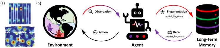
Figure 1: (a) Firing fields of grid cells in various environments from Derdikman et al. [11] (up) and Carpenter et al. [5] (down). The firing pattern changes at the boundary between two regions (fragmentation). (b) Overview of our approach. Given an observation from the environment, the FARMap agent decides whether to fragment the space based on how well it can predict the observation. If fragmentation occurs, the current map (or model) fragment is stored in long-term memory (LTM); the agent then initializes a new map (or model) fragment. Conversely, if the current observation closely matches the observations stored in LTM, the agent loads an existing map (or model) fragment from there (recall). Based on the current fragment, the agent selects an action to explore the environment.

2 Related Work

2.1 Fragmentation of Grid Cell Maps

Mammalian entorhinal grid cells generate highly regular periodic spatial representations that tile open environments [24]. This periodic response is hypothesized to be a general allothetic spatial coordinate system that represents displacements. The spatial response is independent of the speed and direction of movement, and is believed to be formed through integration of self-velocity estimates. However, the regular periodic firing pattern of grid cells becomes fragmented in more complex spatial layouts, such as when an environment contains multiple subdivisions [5, 11, 20]. For instance, there is a fracture in the periodic response at sharp turns of a narrow corridor and in doorways, in which it appears that the grid phase is remapped or jumps discretely to a distinct value at those regions. A recent manuscript [29] builds a model to predict when such discrete remapping events might occur even though the agent explores the environment in a continuous trajectory. They formulated map fragmentation as a clustering computation, and showed how online clustering based on observational surprisal results in fragmentations that match the neuroscientific observations in grid cells and also match normative clustering algorithms like DBSCAN [16]. However, that work did not seriously explore the utility of grid cell-like map fragmentation in the context of function. Here, we show that surprisal-based fragmentation, which fits the biological fragmentation data, is a biologically plausible principle that enables agents to efficiently build maps of various environments in an online way, without getting stuck in local loops.

2.2 Grid Cell-Inspired SLAM

Grid cells have received attention in robotics due to their potential to produce more-robust spatial navigation. Milford et al. [37] propose a model based on continuous attractor dynamics [43] and more recently with grid cells [3, 36], to achieve correct loop closure during noisy odometry. Similarly, Zhang et al. [56] employ growing self-organizing maps inspired by the hippocampus for the same purpose. Yu et al. [53] extend OpenRatSLAM [3] to 3D environments via conjunctive pose cell model that employs 3D grid cell. These methods focus on the error-correcting properties of grid cell dynamics. They do not consider fragmented grid cell maps and the possibility that these map fragments might represent subgoal constructions which could be used for further spatial exploration.

2.3 Frontier-based SLAM

SLAM (simultaneous localization and mapping) agents must efficiently explore spaces to build maps. A standard approach is to define the frontier between observed and unobserved regions of a 2D environment, and then select exploratory goal locations from the set of frontier states [51]. Frontier-based exploration has been extended to 3D environments [9, 12] and used as a building block of more sophisticated exploration strategies [47]. Although conceptually simple, frontier-based exploration can be quite effective compared to more sophisticated decision-theoretic exploration [27]. A cost of frontier-based exploration is the use of global maps and global frontiers, which makes the process memory expensive and search intensive. In contrast to frontier-based exploration, our approach learns the surprising parts of an environment as intrinsic subgoals, selecting among those as the exploratory goals.

2.4 Submap-Based SLAM

Submap-Based SLAM algorithms involve mapping a space by breaking it into local submaps that are connected to one another via a topological graph. Such methods are usually designed to avoid the problems of accruing path integration errors when building maps of large spaces (e.g.SegSLAM [18]) and to reduce the computational cost of planning paths between a start and target position [18, 35]. Segmented DP-SLAM [35] adds DP-SLAM [14] to SegSLAM to reduce the search space, generating segments periodically at fixed time-intervals. Topological SLAM [7] generates new landmarks in an environment to build a topological graph of the landmarks and navigates based on the graph. FARMap is closely related to these methods in that we build multiple submaps. However, FARMap divides space based on properties of the space (how predictable the space is based on the local map or model), and does so in an online manner using surprisal. As we show below, this fragmentation strategy can lead to improvements in performance compared to random or periodic fragmentation.

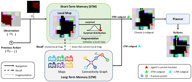
Figure 2: Illustration of the FARMap framework. Navigation (black arrow): Given the current observation which is an ego-centric top-down view with a restricted field of view and previous action, the agent updates its short-term memory (STM) and selects a subgoal from the current local map in STM or the local map connectivity graph stored in LTM. The planner generates a sequence of actions for the shortest-path to the subgoal. Recall (dashed arrow): If the agent arrives at a fracture point (circle in the map), a corresponding local map is recalled from LTM and the current local map stored in LTM is updated. Fragmentation (gray arrow): If the current surprisal is higher than a threshold, the current local map is stored in LTM and a new local map is initialized. $o^{\prime}_{t}$ is a spatially transformed observation with the same size of the current local map to update the map.

3 Fragmentaion and Recall based Spatial Mapping (FARMap)

3.1 Motivation and Overview

Animals explore spaces efficiently even in large environments by grid cells’ remapping that divides an environment into multiple subregions. This remapping can be modeled as surprisal-based online fragmentation [29]. Here, we propose a fragmentation-and-recall based spatial map-building strategy (FARMap) inspired by remapping of grid cells. FARMap tackles the problem of SLAM algorithms is that the memory cost and search cost of finding subgoals grow rapidly with environment size; for agents exploring a very large space, the computational costs could explode.

While exploring an environment, an agent builds a local model (map) and uses it in short-term memory (STM) to compute a surprisal signal that depends on the current observation and the agent’s local model-based prediction. When the surprisal exceeds some threshold, this corresponds to a fragmentation event. At the event, the local model is written to long-term memory (LTM) which builds a connectivity graph that relates model fragments to each other so that it can share information across local models without direct access to the stored models in LTM. Then, the agent initializes an entirely new local model. On the other hand, if the agent revisits the fracture point, the agent recalls the corresponding model fragment (local model). Hence, the agent can preserve and reuse previously acquired information. Figure 2 shows how an agent decides its next subgoal given the observation and the previous action with fragmentation and recall. LTM (except the connectivity graph portion) can be regarded as external memory while STM is modeled as working memory. This external memory is accessed or updated only during fragmentation or recall processes. Consequently, this can be beneficial for machines with limited memory access (see Appendix D). Please refer to Appendix B for overall procedure, and Appendix C for detailed discussions of LTM retrieval overhead.

3.2 Fragmentation and Recall

Fragmentation

Fragmentation occurs if the $z$-scored current surprisal (($s_{t}-\mu_{t})/\sigma_{t})$ exceeds a threshold, $\rho$, where $s_{t}$ denotes surprisal at time $t$, and $\mu_{t}$ and $\sigma_{t}$ mean its running mean and the standard deviation. Initially, on each new map, the agent collects surprisal statistics and is not permitted to further fragment space until the number of samples is greater than $25$ (for large enough sample conditions for statistics). We also store the ratio $q_{c}$ of the number of frontier cells ($N_{\text{frontier}}$) to the number of known cells ($N_{\text{known}}$) and the distance between each fracture point in the current local map $\mathbf{M}^{\text{cur}}_{t}$ that is further explained in this section. The ratio is used for guiding agents on whether or not to move to other local maps. When $\mathbf{M}^{\text{cur}}_{t}$ is stored in LTM, it is connected with adjacent map fragments that share the same fracture point in the connectivity graph. In other words, the node of the graph is a model fragment and a connection denotes that both fragments share a fracture point.

Recall

Each local map records the fracture points. At these points, there are overlaps with other map fragments. When the agent moves to the point in the current local map, the corresponding local map is recalled from LTM and the current one is stored in LTM.

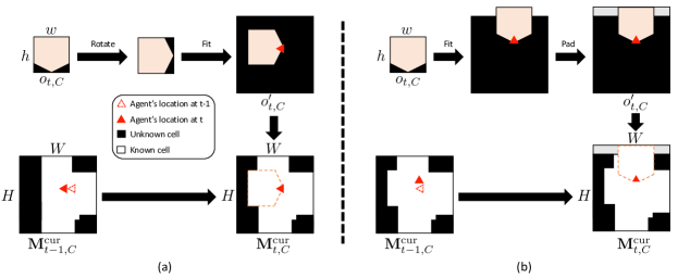
Figure 3: Schematic illustrations of how the local map is updated. In this figure, we only consider the visibility of each cell without considering occupancy and the color for simplification. (a) We first rotate the current observation $o_{t,C}$ based on the head direction of the agent in the local map. Then, the observation is zero-padded to have the same size as the local map. Finally, the local map is updated by adding transformed observation $o^{\prime}_{t,C}$. (b) If the current observation does not fit in the local map due to the agent’s location, we add zero-padding (gray) to both observation and the local map. Hence, the size of the local map has increased ($H$ has changed).

3.3 Local Map

The STM has a local predictive spatial map, $\mathbf{M}_{t}^{\text{cur}}\in\mathbb{R}^{(C+1)\times H\times W}$ where height $H$ and width $W$ grow as the agent extends its observations in the local region by adding newly discovered regions. The first $C$ channels of $\mathbf{M}_{t}^{\text{cur}}$ denote color and the last channel denotes the agent’s confidence in each spatial cell. In this paper, we will focus only on the update of the confidence channel ($C$-th channel). The local predictive map is simply a temporally decaying trace of recent sensory observations like a natural agent [55]:

$$\mathbf{M}^{\text{cur}}_{t,C}=\gamma\cdot\mathbf{M}^{\text{cur}}_{t-1,C}+(1-\gamma)\cdot o^{\prime}_{t,C},$$ (1)

where $\gamma$ is a decay factor and $o_{t}\in\mathbb{R}^{(C+1)\times h\times w}$ is the egocentric view input observation in the environment at time $t$ sized as $(h,w)$. The last channel of the observation means visibility caused by occlusion or restricted field of view (FOV); visible (1) or invisible (0) on each cell. The red region is visible and others are invisible in Figure 2. $o^{\prime}_{t}\in\mathbb{R}^{(C+1)\times H\times W}$ denotes a spatially transformed observation to $\mathbf{M}^{\text{cur}}_{t-1}$ to update the current observation to the local map in the correct position; rotation and zero-padding. Figure 3 shows a toy illustration of how to transform the current observation to update the local map and how the map size grows. We first rotate the observation following the head direction of the agent in the map and then zero-pad it so that it has the same size as the local map considering the agent’s current location in the map. If the observation does not fit in the same size of the map due to the agent’s location, we add zero-padding (gray in the figure) to both the transformed observation and the local map. Then, we update the local map by adding the transformed observation.

3.4 Surprisal

The surprisal works as a criterion of fragmentation, which can be any uncertainty estimate of the future, such as negative confidence or future prediction error. We employ the local predictive map for measuring surprisal. The scalar surprisal signal $s_{t}=1-c_{t}$ is generated using the local map in STM and the current observation, where $c_{t}$ quantifies the average similarity of the visible part of observation to the local predictive map $\mathbf{M}^{\text{cur}}_{t-1}$ before update:

$$c_{t}=\frac{\mathbf{M}^{\text{cur}}_{t-1,C}\cdot o^{\prime}_{t,C}}{||o^{\prime}_{t,C}||_{1}}.$$ (2)

The agent is assumed to maintain a running estimate of the mean $\mu_{t}$ and standard deviation $\sigma_{t}$ of past surprisals, stored as part of the current map.

3.5 Subgoal

Subgoals are decided by using either the current local map in STM or the connectivity graph in LTM. The former enlarges the current local map while the latter helps find the next local map to explore. An agent explores the local region in the environment unless the current surprisal is too low (e.g., $z$-score is smaller than $-1$) and there is a less explored local map nearby.

Subgoals made with the current local map are based on frontier-based subgoals [51] for exploring the local region. Each cell in the region is categorized as known and unknown based on whether it was previously observed or not, and occupied and unoccupied (empty) based on its occupancy. In the current local map, we first find all frontiers which are unknown cells adjacent to the known unoccupied cells. A group of consecutive frontiers is called a ‘frontier-edge’ and [51] uses the nearest centroid of the frontier-edge as a subgoal. Unlike standard SLAM methods that employ the entire map, our map in STM only covers a subregion of the environment. After fragmentation, the region where the agent came from, has several frontiers (border of two local models) forming a frontier-edge. It leads the agent to go back to the previous area and recall the corresponding map fragment. This would lead to the agent moving between two map fragments for a long time. Hence, we prioritize the frontier-edge that is not located spatially behind the agent. The subgoal is sampled with the following weight $w_{i}$ for each frontier-edge $\mathcal{F}_{i}$:

$$w_{i}=\frac{|\mathcal{F}_{i}|\cdot\mathbbm{1}(\mathcal{F}_{i}\text{ is not located spatially behind the agent})}{d_{i}},$$ (3)

where $d_{i}$ means the distance between the current position and the centroid of $\mathcal{F}_{i}$ and $\mathbbm{1}(\cdot)$ is the indicator function that is 1 if the condition is true otherwise 0.

Once the agent finishes mapping the local region, it should move to different subregions. However, subgoals from the current local map can misguide the already explored region since the agent does not have information beyond the map. Hence, we employ the connectivity graph of local maps stored in LTM. We leverage the discovery ratio (the ratio of the number of frontier cells to the number of known cells) $q$ mentioned above to find the most desirable subregions to explore. We also utilize the Manhattan distance between the current agent location and the fracture point between the current ($c$-th) local map and the connected $i$-th local map, $d_{i,c}$ where $d_{c,c}=0$ and $d_{j,c}=\infty$ if $j$-th local map is disconnected to the current map. Then, the desirable local map is selected as

$$g=\operatorname*{arg\,max}_{i}\frac{q_{i}}{d_{i,c}+\epsilon},$$ (4)

where $\epsilon$ denotes the preference of staying in the current local map; a smaller value encourages staying in the current local map. If $g$ is not equal to $c$, the fracture point between the current local map and $g$-th local map is set to the subgoal. Once the agent arrives at the fracture point, the corresponding local map is recalled and the agent recursively checks Eq. (4) until $g$ is the arrived subregion. Note that the distances between a new location and other fracture points stored in the recalled local map are precomputed since they are fixed.

3.6 Planner

The planner takes a subgoal and the current spatial map in STM and finds the shortest path within the map from the current agent location to the subgoal. We use Dijkstra’s algorithm for planning a path to the next subgoal. However, the planner can be any path planning method such as A^∗ algorithm [25] or RRT [32].

(a) Observation

(b) Small (size: 3249)

(c) Medium (size: 13689)

(d) Large (size: 23868)

Figure 4: Environments. Empty cells (that can be occupied by the agent) are black; walls are randomly colored. (a) Top-down visualization of the agent’s local field of view (FOV) (agent: red triangle; shaded region: observation) within an environment (b). The agent has only a locally restricted egocentric view. The right side is occluded by a wall. (b) Top-down view of one environment. The red box marks the region shown in (a). (c), (d) Examples of medium and large environments.

4 Procedurally-Generated Environment

We build a procedurally-generated environment for the map-building experiments. Figure 8 and Algorithm 2 in Appendix show the procedure of map generation. We first generate grid-patterned square rooms and randomly connect and merge them. Then, we flip boundary cells (empty or occupied) multiple times for diversity. Formally, given the length of square $S$, the interval between square rooms, $L$, and the size of the grid, $(N,M)$, we first generate the binary square grid map $\mathcal{M}\in\{0\text{(empty)},1\text{(occupied)}\}^{(N\cdot S+(N+1)\cdot L)\times(M\cdot S+(M+1)\cdot L)}$. Let $s_{i}$ be the $i$-th square as a row-major order in $\mathcal{M}$. For each of the adjacent square pairs, we connect two squares with probability $p_{\text{connect}}$ as a width $w\sim\text{unif}\{1,2,\dots,S-1\}$ or merge (special case of connect with width $S$) them with probability $p_{\text{merge}}$. Then, we flip all boundaries between occupied and empty cells $K$ times with probability $p_{\text{flip}}$. After flipping the boundaries, there are several isolated (i.e. not connected to other submaps) submaps in $\mathcal{M}$. We only use the submaps where the sizes are greater than a threshold ($3S^{2}$ in our implementation). After creating maps, we randomly colorize each occupied cell and scale up by a factor of 3. Note that the proposed environment has very complex maps. Please refer to the attached environment generation code for more details.

Figure 4 shows examples of environment and observation. The walls in the environment are randomly colored and are composed of various narrow and wide pathways. For each trial, the agent is randomly placed before it begins to explore the environment. Figure 4(a) illustrates an example of the agent’s view in the small environment shown in Figure 4(b). The agent is presented as a red triangle and the observed cells are shaded. The agent has the restricted field of view with occlusion ($130^{\circ}$).

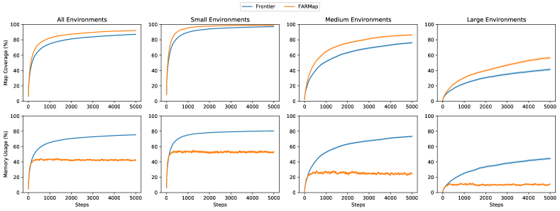
Figure 5: Growth in agent-explored map region as a function of the number of steps in the environment matches the performance of an augmented Frontier-based baseline with less memory use. Mean spatial map coverage performance (up) and mean memory usage (down) as a function of the number of steps taken in various sizes of environment sets. FARMap achieves better or comparable exploration as a Frontier-based exploration baseline (Frontier) [51]. while using only about half the memory on average. The memory benefit is increased in a larger environment.

5 Experiments

In this section, we conduct experiments for FARMap comparing with its baselines on the proposed procedurally generated map environments and robot simulations. We conduct experiments on dynamic environments, an ablation study, and sensitivity analysis of hyperparameters in Appendices F,  H and I, respectively. To quantify the difficulty of the proposed environments for the RL exploration algorithm, we measure the performance of RND [4] in the environments in Appendix J.

We measure the map coverage, memory usage, and wall-clock time for each environment at each time step as our evaluation criteria and calculate the mean and standard deviation over all runs. The memory usage in each environment is calculated as a ratio of the local map size (memory size, $H\times W$) to the environment size. Note that the local map size is the asymptotically dominant factor in the memory. We compare FARMap with standard frontier-based exploration (Frontier) [51]. Please refer to Appendix E for the experimental settings.

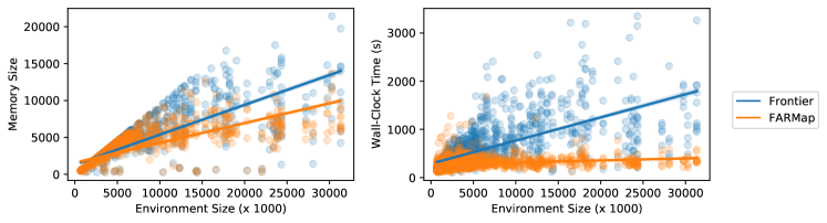
Figure 6: Relative memory and wall-clock time advantage of FARMap to Frontier grow with environment size. Comparison of memory cost (left) and wall-clock time (right) as a function of environment size (circles: experimental results; line: linear regression fit). FARMap requires substantially less memory and is much faster than other methods.

5.1 FARMap in Procedurally-Generated Environments

Figure 5 summarizes the performance over the course of exploration on 1,500 environments with three groups based on their sizes; small (size < 5,000), medium (5,000 $\leq$ size < 15,000), and large (size $\geq$ 15,000). The lines in the plots are the average of all or a group of experiments and the shaded areas are standard errors of the mean which are not visible due to a large number of trials. FARMap clearly outperforms the baseline on every step, which means that it explores the environment more efficiently. On the other hand, FARMap generally uses a stable amount of memory on average (40 %) over all experiments while Frontier requires much more memory as map coverage increases. The average memory usage of FARMap is almost consistent in any group of environments as the agent explores environments while the usage of Frontier keeps increasing.

Figure 6 and Table 1 analyze memory size and wall-clock-time changes depending on the environment size. The memory usage of FARMap in each environment is measured by the biggest memory size during exploration since the size is dynamically changed by fragmentation and recall. FARMap clearly outperforms the baseline with a much less wall-clock time while planning. This is because our agent only refers to the subregion of the environment not using the entire map. Especially in large environments, it is approximately four times faster than the baseline. Moreover, FARMap requires less memory than the baseline as we mentioned above. The high confidence intervals are caused while aggregating results from multiple high-variance environments (see Appendix G). We also measure the ratios of memory usage and map coverage and of wall-clock time and map coverage in Table 7. The result shows that FARMap has a smaller ratio in all criteria, which means that it requires fewer time and memory resources to explore 1% of environments.

Table 1: Comparison of average map coverage (%), memory use (%), and wall-clock time ($s$) for medium, and large environments. The memory usage advantage of FARMap relative to its counterpart grows with environment size. The numbers in parentheses are 95 % confidence intervals generated by bootstrap with one million samples.

Model	Medium (5,000 $\leq$ size $<$ 15,000)			Large (size $\geq$ 15,000)
	Coverage	Memory	Time	Coverage	Memory	Time
Frontier [51]	76.3 (15.6, 99.8)	73.3 (13.0, 92.3)	871.9 (290, 2020)	41.4 (6.1, 84.3)	44.4 (3.8, 84.3)	1261.0 (217, 3189)
FARMap	86.4 (15.6, 100.0)	62.9 (12.5, 90.2)	321.4 (191, 528)	56.6 (6.1, 97.7)	31.4 (3.8, 54.3)	352.5 (202, 633)

5.2 FARMap in Robot Operation Simulation

We simulate FARMap in four continuous environments with turtlebot3 (burger) via Robot Operation System (ROS) [34] with Gazebo simulator. ROS is one of the standard libraries for conducting robotic experiments, and it allows for straightforward deployment to real robots at no additional cost. Unlike experiments performed in Section 5.1, the observation here involves a 360-degree first-person view via the default laser scan. We utilize the default global planner in the ‘move_base’ package. Frontier and FARMap are tested in four continuous 3D environments with a fixed starting location (Figure 7), for 2500 steps using five different random seeds. The laser scan operates at a frequency of 2.5Hz, meaning that the agent updates the local map every 0.4 seconds.

Table 2 presents a comparison between FARMap and Frontier in terms of map coverage and memory usage measurements without any normalization. We do not use wall-clock time for the comparison as it is now related to the agent step. In most environments, FARMap has better exploration performance. Although FARMap consumes more memory than Frontier in AWS Office, its memory-to-coverage ratio is better than Frontier’s (1.16 compared to 1.26, respectively).

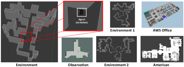
Figure 7: Robot simulation environment. The turtlebot agent moves around with a 360-degree laser scan sensor to map the entire space.

Table 2: Coverage (k) of each ROS environment. FARMap has better performance in 3D robot simulation environment 1, AWS Office and American while it has similar performance in environment 2. The number in parenthesis denotes a 95% confidence interval.

Model	Environment 1		Environment 2		AWS Office [15]		American [45]
	Coverage (k)	Memory (k)	Coverage (k)	Memory (k)	Coverage (k)	Memory (k)	Coverage (k)	Memory (k)
Frontier	7.0 ($\pm$ 1.4)	20.5 ($\pm$ 1.0)	8.3 ($\pm$ 0.6)	32.8 ($\pm$ 34.4)	38.2 ($\pm$ 30.0)	48.1 ($\pm$ 20.8)	13.8 ($\pm$ 3.1)	11.0 ( $\pm$ 2.1)
FARMap	7.7 ($\pm$ 1.0)	20.1 ($\pm$ 2.4)	8.3 ($\pm$ 0.1)	23.0 ($\pm$ 8.6)	57.0 ($\pm$ 4.7)	66.0 ($\pm$ 14.3)	15.8 ($\pm$ 4.2)	10.6 ($\pm$ 3.7)

5.3 FARMap with Neural SLAM

We conducted experiments on both FARMap and Frontier integrated with the pre-trained Neural SLAM [6] obtained from the official repository for the Gibson [45] exploration task with the Habitat simulator [49]. We use ‘American’ used in Section 5.2 as an example. For the fair comparison with FARMap and Neural SLAM, we replaced the global policy in FARMap or Frontier to establish the ‘long-term goal’, following Chaplot et al. [6]. This essentially means that we employ a Neural SLAM module to convert RGB observations to a 2D map and a Local Policy to generate discrete actions based on the given global goal. Table 3 demonstrates that Neural SLAM, when substituting FARMap for global policy, attains superior exploration performance. In contrast, incorporating Frontier led to a decrement in performance. These experimental outcomes also hint at the potential advantages of applying our fragmentation-and-recall concept to exploration methods that leverage maps.

Table 3: Comparison of Neural SLAM and its adaptations with Frontier and FARMap on the Gibson American environment.

Model	% Cov.	Cov. (m2)
Neural SLAM [6]	0.818	64.795
Neural SLAM w/o global policy + Frontier	0.733	58.103
Neural SLAM w/o global policy + FARMap	0.833	66.012

6 Discussion

We proposed a new framework for exploration based on local models and fragmentation, inspired by how natural agents explore space efficiently via grid cells’ remapping. Our framework fragments the exploration space based on the current surprisal in real time and stores the current model fragment in long-term memory (LTM). Stored fragments are recalled when the agent returns to the state where the fragmentation happened so that the agent can reuse the local information. Accordingly, the agent can refer to longer-term local information. We believe that the framework can be applied to any tasks that use streaming observations or data which are reused or recurring. We applied this to the setting of spatial exploration. The surprisal is generated by short-term memory (STM) using a local map in FARMap. Consequently, FARMap requires less wall-clock time and memory, and a smaller number of actions than the baseline method [51] with even improved map-building performance in both static and dynamic discrete environments, and continual robot simulations. Our paper aims to be a proof-of-concept for fragmentation and recall in spatial map-building using frontier-based exploration and Neural SLAM but we believe that this concept can be applicable to other exploration paradigms and various applications. This concept can make large-scale exploration, which typically requires a huge memory size and long-ranged memory span, significantly more efficient.

Appendix

A Additional Related Works

A.1 Graph-Based SLAM

Graph-based SLAM [23, 30, 52] constructs topological graph for efficient exploration by reducing the dimensionality of planning problem. Once this graph is established, a planner utilizes it to navigate toward subgoals. GBPlanner [30, 52] creates a random graph in the local region and uses it for path planning. This reduces computational cost for local path planning by reusing sparse graph nodes although it still uses frontier. In contrast, FARMap aims for efficient exploration in terms of memory, time, and the number of steps by dividing the environment (i.e., fragmentation) and the topological graph is used for moving one subregion to another. We believe that there is a potential synergy between graph-based SLAM and FARMap. Such synergy can be achievable by substituting frontier-based exploration with a graph-based approach, pairing global fragmentation from FARMap with relatively local planning from graph-based methods.

A.2 Memory-Based Reinforcement Learning

Although the reinforcement learning (RL) algorithm is beyond the scope of this paper, FARMap is similar to memory-based RL in the sense that uses memories. Hung et al. [28] combine LSTM [26] with external memory, along with an encoder and decoder for the memory. Ritter et al. [41, 42] use DND [39] to store the states of LSTM with its inputs and retrieve old states to update the state of LTM in meta-reinforcement learning tasks. Similarly, MRA [19] use working memory and an episodic memory structure but employs an output of the episodic memory as an input for the working memory. On the other hand, HCAM [31] utilize a hierarchical LTM with chunks and attention for long-term recall inspired by Transformers [50] however, their chunks are formed periodically rather than based on content and are not used as intrinsic options for exploration. Our spatial map-building framework is similar to memory-based RL methods in terms of having two memory architectures inspired by the brain. However, FARMap fragments an environment (or space) in an online manner and recalls stored memories inspired by grid cells, while memory-based RL stores previous states. Moreover, we use the connectivity graph of STMs to find the next subgoal for efficient map building. We would like to emphasize that FARMap is not a reinforcement learning method. On the other hand, we believe that our proposed concept, fragmentation-and-recall can be applicable to memory-based reinforcement learning by reducing search space in the memory.

Algorithm 1 FARMap Procedure at time $t$. FARMap algorithm is colored in blue on top of Frontier algorithm [51].

1:a spatial map $\mathbf{M}_{t-1}^{\text{curr}}$, previous action $a_{t-1}$, current observation $o_{t}$, short-term memory STM, long-term memory LTM, position at time $t$, $\textsf{pos}_{t}$, decay factor $\gamma$, fragmentation threhsold $\rho$ and hyperparameter $\epsilon$.

2:Updated map, $\mathbf{M}_{t}^{\text{curr}}$ and a sequence of actions $\{a\}$

3:procedure Step

4:     $\mathbf{M}_{t}^{\text{curr}}=\gamma\cdot\mathbf{M}_{t-1}^{\text{curr}}+(1-\gamma)\cdot o^{\prime}_{t}$ $\triangleright$ Update the current local map

5:     Calculate $s_{t}=1-c_{t}$ following Eq. (2).

6:     $z_{t}=(s_{t}-\mu_{t})/\sigma_{t}$

7:     $q_{c}$ =$N_{\text{frontier}}$ / $N_{\text{known}}$

8:     if $\textsf{pos}_{t}=$ fracture point then$\triangleright$ Recall

9:         $\textsf{LTM}\leftarrow\textsf{Store}(\textsf{pos}_{t},q_{c},\mathbf{M}_{t}^{\text{curr}})$ $\triangleright$ Store $\mathbf{M}_{t}^{\text{curr}}$

10:         $\textsf{STM}\leftarrow\textsf{Recall}(\textsf{pos}_{t};\textsf{LTM})$ $\triangleright$ change $\mathbf{M}_{t}^{\text{curr}}$

11:     else if $z_{t}>\rho$ then $\triangleright$ Fragmentation

12:         $\textsf{LTM}\leftarrow\textsf{Store}(\textsf{pos}_{t},q_{c},\mathbf{M}_{t}^{\text{curr}})$

13:         Initialize a new map $\mathbf{M}_{t}^{\text{curr}}$ in STM.

14:     end if

15:     Update running mean $\mu_{t+1}$ and standard deviation $\sigma_{t+1}$ of surprisal.

16:     $g=\operatorname*{arg\,max}_{i}\frac{q_{i}}{d_{i,c}+\epsilon}$ $\triangleright$ Eq. (4)

17:     if $g\neq c$ then $\triangleright$ Subgoal based on connectivity between fragments.

18:         subgoal $\leftarrow$ the fracture point between the current fragment $c$ and a fragment $g$

19:     else

20:         Find frontier-edges $\{\mathcal{F}_{i}\}$ and their centroids $\{\text{centroid}_{i}\}$.

21:         $d_{i}=||\textsf{pos}_{t}-\text{centroid}_{i}||_{1}$.

22:         $w_{i}=1/d_{i}\cdot$ $|\mathcal{F}_{i}|\cdot\mathbbm{1}(\mathcal{F}_{i}\text{ is not located spatially behind the agent})$

23:         $\triangleright$ $\mathbbm{1}(\cdot)$ is 1 if the condition is true else 0.

24:         Select frontier-edge $\mathcal{F}_{g}$ based on the weighted sampling with $\{w_{i}\}$.

25:         subgoal $\leftarrow$ the nearest frontier $\in\mathcal{F}_{g}$ from its centroid.

26:     end if

27:     A sequence of actions, $\{a\}\leftarrow$ Planner(subgoal; $\mathbf{M}_{t}^{\text{curr}}$) $\triangleright$ Dijkstra’s algorithm.

28:end procedure

B Overall Procedure of Spatial Navigation

Algorithm 1 presents the overall procedure of FARMap at time $t$. On top of the Frontier algorithm [51], we colored the FARMap algorithm blue. Given the previous action $a_{t-1}$, current observation $o_{t}$, a local predictive map $\mathbf{M}_{t-1}^{\text{curr}}$, we first update the map following Eq. (1) and calculate the surprisal $s_{t}$ following Eq. (2).

If the agent is located in the fracture point where fragmentation happened between the current local map, $\mathbf{M}_{t}^{\text{curr}}$ and another local map stored in LTM (Line 8), we store $\mathbf{M}_{t}^{\text{curr}}$ and $q_{c}$ in LTM, and the stored map fragment is recalled to STM. On the other hand, if the $z$-scored surprisal $z_{t}$ calculated with running mean and standard deviation of surprisal within the current local map is greater than a threshold, $\rho$ (Line 11), we store $\mathbf{M}_{t}^{\text{curr}}$, and $q_{c}$ in LTM, and initialize a new map in STM. During this process, the current locations in both $\mathbf{M}_{t}^{\text{curr}}$ and a new map are marked as fracture points.

After checking recall and fragmentation, we find the desirable local map fragments that are less explored than other fragments as mentioned in Section 3.5. If the current map is not the desirable map, we set the subgoal as the fracture point between the current map and the desirable map. Otherwise, we first find frontier-edges and calculate the weight of each frontier-edge $\mathcal{F}_{i}$ using weighted sampling with weight $w_{i}$ following Eq. (3) ($w_{i}$ is $1/d_{i}$ in the case of the Frontier model). The subgoal is defined as the nearest frontier from the centroid of the sampled frontier-edge. Finally, a planner generates a sequence of actions to navigate to the subgoal. Note that while the agent moves based on the sequence, it keeps updating the map and checking fragmentation and recall.

C LTM Retrieval Overhead

FARMap needs to consider the retrieval time of LTM since it is not located in the main memory. If the memory (RAM) is larger than the environment so that we can even use LTM on RAM, retrieval time is not a concern, and FARMap is useful in boosting speed, although it might use more memory. In our original scenarios, LTM is an external memory (non-volatile memory). Usually, SSD’s speed (including bandwidth and read/write) is around 300-600 MB/s while RAM (DDR4) operates on 5-25 GBps. In this case, SSD read/write can be a bottleneck. However, the flash memory speed is around 5 GBps, and the retrieval time for the map will be negligible compared to the planning time. It is generally not recommended to use a hard disk drive (HDD), whose data transfer rate is around 100 MB/s.

D Potential Applications

In this section, we introduce several potential applications where FARMap will be helpful by reducing memory and time cost.

D.1 Mars Exploration

Mars exploration rovers such as Opportunity and Curiosity have limited resource. For example, the Curiosity rover has 256 MB RAM with 2GB flash memory. However, the mission range on Mars may be much larger than the RAM. Therefore, efficient mapping is required and we believe that FARMap will be helpful in Mars exploration.

D.2 2D/3D Mapping with LiDAR

As mentioned in Section 5.2, FARMap is capable of utilizing observations from LiDAR for map-building in continuous environments. The resolution of the sensor can be set to a cell unit. Considering the property of the Robot Operating System (ROS) [34], we believe that FARMap can be easily deployed to a real robot. Additionally, it is feasible to extend to 3D by using 3D voxel mapping instead of 2D pixel mapping. This approach can prove beneficial in large-scale environments such as buildings, airports, and houses.

E Experimental Details

Our models are implemented on PyTorch and the experiments are conducted on Intel(R) Xeon(R) CPU E5-2650 v4 @ 2.20GHz for spatial exploration experiments and NVIDIA Titan V for RND and Neural SLAM.

E.1 FARMap Environment Generation

To generate the environment, we run map generation (Algorithm 2) 200 times and then use the 300 largest-sized maps. All maps are scaled up by a factor of 3 after colorization for the task. On every trial, we sample $S$ and $N$ from $\{3,4,5,6,7\}$ and set $M=N$. $K,L\in\mathbb{N}$ are sampled from $[0,10]$ and $[1,3]$, respectively. We set $p_{\text{connect}}$, $p_{\text{merge}}$ and $p_{\text{flip}}$ to $0.25,0.25,0.05$, respectively. Figure 8 illustrates the procedure of environment generation mentioned in Algorithm 2. Table 4 shows the statistics of the size of the generated environment. We also attached examples of generated environments in the repository.

E.2 FARMap

We run the agent on 1500 different environments: 300 different maps with five random seeds and the starting position and the color of the map are changed on each random seed. We set $\gamma$, $\rho$, and $\epsilon$ to 0.9, 2, and 5, respectively. The observation size $(h,w)$ is (15,15). If the frontier-based exploring agent is surrounded by a large frontier-edge in an open space, the centroid of the frontier can fall into the interior of the explored space, leading to no new discovery. This causes the agent to become stuck. We improve the agent by selecting the nearest unoccupied cell from the nearest frontier state from the centroid.

Algorithm 2 Spatial Exploration Environment Generation

1:$N,M,L,S,K,p_{\text{connect}},p_{\text{merge}},p_{\text{flip}}$

2:A set of maps, $\{\mathcal{M}\}$.

3:procedure MapGeneration

4:     Initialize $\mathcal{M}\in\{0,1\}^{(N\cdot S+(N+1)\cdot L)\times(M\cdot S+(M+1)\cdot L)}$, $(N,M)$ grid with interval $L$ and each square sized $(S,S)$. $\triangleright$ Figure 8 (1).

5:     for $(s_{i},s_{j})\in\{(s_{i},s_{j})|s_{i}\text{ and }s_{j}\text{ are adjacent},i\leq j\}$ do $\triangleright$ Get adjacent grid square pairs.

6:         $x\sim\mathcal{B}(1,p_{\text{connect}})$ $\triangleright$ Connect adjacent squares with probability $p_{\text{connect}}$.

7:         if $x=1$ then

8:              $w\sim\text{unif}\{1,\dots,S-1\}$

9:              Connect $s_{i}$ and $s_{j}$ with width $w$. $\triangleright$ Figure 8 (2).

10:         end if

11:         $x\sim\mathcal{B}(1,p_{\text{merge}})$ $\triangleright$ Merge adjacent squares with probability $p_{\text{merge}}$.

12:         if $x=1$ then

13:              Merge $s_{i}$ and $s_{j}$ by removing the interval. $\triangleright$ Figure 8 (3).

14:         end if

15:     end for

16:     for $k\leftarrow 1$ to $K$ do

17:         for $c\in\{c|c\in\mathcal{M},\exists_{c^{\prime}}\ c\textsf{ xor }c^{\prime}=1,c^{\prime}\in\text{Adj}(c)\}$  do $\triangleright$ Get boundary cells in the map.

18:              $x\sim\mathcal{B}(1,p_{\text{flip}})$ $\triangleright$ Flip the cell with probability $p_{\text{flip}}$.

19:              $c=c\ \textsf{xor}\ x$ $\triangleright$ Figure 8 (4)-(6).

20:         end for

21:     end for

22:     Divide $\mathcal{M}$ into a set of isolated maps $\{\mathbf{m}_{i}\}$ $\triangleright$ Figure 8 (7).

23:     Filter out a map in $\{\mathbf{m}_{i}\}$, where the size is smaller than $3S^{2}$.

24:     Randomly colorize the occupied cell in each map. $\triangleright$ Figure 8 (8).

25:     Scale up each map in $\{\mathbf{m}_{i}\}$ by factor of 3.

26:end procedure

Table 4: The statistics of the size of environments in the dataset.

Statistics	All	Small	Medium	Large
The number of environments	1500	1015	345	140
Average size	5697.8	2466.7	8532.4	22138.7
Standard deviation of size	6265.8	1253.7	2828.5	4872.9

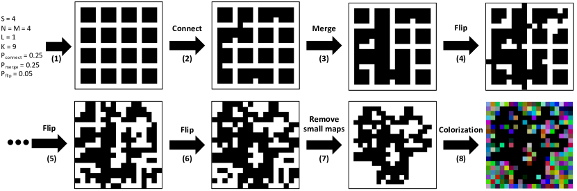
Figure 8: Procedure of map generation. (1) We first set square grid where black and white denote empty and occupied, respectively. (2) We randomly connect and (3) merge adjacent grid. (4)-(6) We also randomly flip the boundaries of empty and occupied cells recursively. (7) Then, we remove small isolated subregions and (8) randomly colorize occupied cells. Finally, we increase the size of the map.

E.3 RND

We train RND [4] for 1 million steps without extrinsic reward for each environment. RND is based on recurrent PPO [44]. Table 5 shows the architecture of RND used for the experiments. The learning rate is 0.0001, the reward discount factor is 0.99 and the number of epochs is 4. For other parameters, we use the same values mentioned in PPO and RND: we set the GAE parameter $\lambda$ as 0.95, value loss coefficient as 1.0, entropy loss coefficient as 0.001, and clip ratio ($\epsilon$ in Eq. (7) in [44]) as 0.1.

Table 5: The architecture of RND agent. The networks are divided into the policy module and RND module.

Policy module	RND module
Conv2d (8$\times$8, 16)	Conv2d (8$\times$8, 32)
Conv2d (4$\times$4, 32)	Conv2d (4$\times$4, 64)
FC (3200$\times$512)	Conv2d (3$\times$3, 64)
LSTM (512, 512)	FC (3136$\times$512)
FC (512$\times$5) $\times$ 2	FC (512$\times$512)
FC (512$\times$1) $\times$ 2	FC (512$\times$512)

Table 6: All methods have stable performance in dynamic environments. We measure average map coverage (%), memory use (%), and wall-clock time (s) for dynamic environments with 95% confidence intervals computed by bootstrap with one million samples. ^†: the memory usage of RND is calculated by the ratio between the number of parameters (7.7M) and each environment size.

Method	Coverage (%)	Memory (%)	Time (s)
Frontier [51]	95.0 (72.2, 100.0)	86.6 (64.5, 90.0)	742.2 (385.6, 1361.7)
FARMap	95.5 (72.5, 100.0)	67.9 (37.0, 89.6)	386.0 (154.5, 521.7)

F Dynamic Environment

Inspired by Random Disco Maze [1], we build Medium-sized 345 dynamic environments where the wall colors are changing every time step. Table 6 shows that all methods work well in the environments, and FARMap is still more efficient than its baselines in terms of memory and wall-clock time.

Table 7: Comparison of the ratios of memory usage and map coverage, and of wall-clock time and map coverage. Smaller value denotes the model is more efficient than others. FARMap has the smallest ratios in all comparisons.

Model	Small		Medium		Large
	Memory / Coverage	Time /Coverage	Memory /Coverage	Time / Coverage	Memory /Coverage	Time / Coverage
Frontier	0.83	3.71	0.96	11.43	1.07	30.46
FARMap	0.80	3.52	0.73	3.72	0.55	6.22

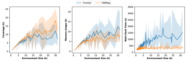
Figure 9: Map coverage, memory usage, and wall-clock time advantage of FARMap to Frontier grow with environment size. Comparison of these metrics as a function of environment size. The mean (line) and 95% confidence interval (shade) are calculated by bootstrap with one million samples each from 150 groups (10 environments each) ordered by size.

G Wide Confidence Intervals

In Table 1, 95% confidence intervals of each measurement are generated by bootstrap with one million samples. The confidence intervals are very wide since our metrics map coverage, memory usage, and wall-clock time depend on the size and the complexity of the environment, and each method is evaluated on many varied environments as shown in Table 4.

We also present results with much smaller groups in Figure 9. We first sort the environments based on their sizes, and then we partition the environments into 150 groups, each of size 10, and calculate the average with bootstrapping to get a 95 % confidence interval for each group. The 95% confidence intervals measured by bootstrap are also smaller than the reported range in Table 1. Especially, FARMap has a relatively steady wall-clock time across the entire environments while Frontier requires more time with high variance depending on the environments. Although the gaps between FARMap and Frontier in all metrics are small in small environments, as the environment size grows, it becomes larger. In other words, FARMap is better than Frontier in all environments in terms of map coverage, memory usage, and wall-clock time.

H Ablation Study

Table 8 illustrates the ablation study of components of FARMap. Each component contributes to improving the performance while it increases memory and time which are ignorable compared to the baseline performance (44.4, 1261.0, respectively). We also evaluated FARMap, random fragmentation, and uniform fragmentation methods on top of FARMap. This is to demonstrate that surprisal produces effective fragmentations that maintain the exploration performance with low memory and fast wall-clock time. Random and Uniform models only change the fragmentation criteria and other parts (e.g., LTM, subgoal selection, and planning). Table 9 shows that there is a trade-off between frequency of fragmentation and memory usage and wall-clock time. FARMap achieves better exploration performance than random and uniform fragmentation models.

Table 10 shows Frontier and FARMap with RRT planner [32] in large environment. Although the performance gaps between two models are decreased, FARMap still outperforms Frontier.

Table 8: Ablation study for each component in large environments. We chose the best-performed fragmentation threshold without the $z$-score variant in $[0.1,0.9]$.

$z$-score	LTM subgoal	Coverage	Memory	Time
-	-	51.7 (22.1, 90.5)	20.8 (10.0, 49.6)	177.3 (121.7, 254.8)
✓	-	52.8 (21.9, 85.6)	30.4 (15.3, 57.7)	302.3 (167.9, 519.2)
✓	✓	56.6 (6.1, 97.7)	31.4 (3.8, 54.3)	352.5 (202.0, 633.0)

Table 9: Comparison of vanilla FARMap and FARMap with random, and uniform fragmentation in Large Environments. The random model decides to fragment with probability on every time step and the uniform model makes a fragmentation on every Interval step ($L$)

Model	Coverage	Memory	Time
FARMap	56.6 (6.1, 97.7)	31.4 (3.8, 54.3)	352.5 (202, 633)
Random ($P=0.1$)	45.2 (15.4, 82.3)	7.8 (4.4, 13.2)	111.3 (70.9, 141.0)
Random ($P=0.05$)	47.5 (18.0, 87.4)	12.1 (6.7, 20.0)	136.5 (179.8)
Random ($P=0.01$)	49.0 (18.6, 87.6)	24.5 (12.9, 43.7)	290.7 (148.1, 499.6)
Random ($P=0.005$)	49.1 (20.5, 89.6)	30.5 (16.1, 60.0)	378.1 (201.7, 637.7)
Random ($P=0.001$)	54.1 (23.5, 92.4)	46.1 (20.9, 81.4)	683.4 (292.3, 1484.4)
Uniform ($L=25$)	49.1 (15.8, 82.5)	7.5 (4.7, 11.8)	110.8 (84.6, 143.7)
Uniform ($L=50$)	48.8 (17.3, 89.5)	12.6 (6.8, 20.9)	147.3 (112.9, 200.8)
Uniform ($L=100$)	48.3 (18.7, 88.8)	19.3 (10.7, 32.1)	216.5 (150.3, 330.2)
Uniform ($L=200$)	48.8 (22.0, 90.0)	27.5 (14.0, 45.5)	322.2 (209.1, 612.0)
Uniform ($L=500$)	52.2 (22.0, 90.0)	38.2 (16.5, 82.5)	484.2 (292.9, 840.6)
Uniform ($L=1000$)	53.4 (22.1, 91.9)	46.5 (23.4, 87.9)	712.3 (380.6, 1425.0)

Table 10: Comparison of average map coverage (%), memory use (%), and wall-clock time ($s$) in large environments. Both Frontier and FARMap use RRT [32] planner.

Model	Coverage	Memory	Time
Frontier [51]	46.9 (20.7, 94.0)	49.7 (22.6, 90.3)	880.9 (395.6, 1673.1)
FARMap	50.9 (17.3, 91.3)	30.4 (13.8, 55.7)	318.1 (174.6, 500.6)

Table 11: Sensitivity analysis about fragmentation threshold, $\rho$ in FARMap. The numbers in parentheses are the standard deviation.

$\rho$	Small (size $<$ 5,000)			Medium (5,000 $\leq$ size $<$ 15,000)			Large (size $\geq$ 15,000)
	Coverage	Memory	Time	Coverage	Memory	Time	Coverage	Memory	Time
1.0	99.1	71.5	117.9	87.1	39.6	146.2	60.9	17.9	148.4
1.5	99.1	75.7	158.0	87.6	50.2	180.1	59.7	23.3	188.9
2.0 (ours)	99.0	79.1	278.2	86.4	62.9	321.4	56.6	31.4	352.5
2.5	98.8	80.7	207.1	89.0	79.7	557.3	58.4	56.9	770.5
3.0	98.8	81.5	296.1	91.0	85.0	698.2	60.9	67.9	1068.0

Table 12: Sensitivity analysis about decaying factor, $\gamma$ in Eq. (1). The numbers in parentheses are the standard deviation.

$\gamma$	Small (size $<$ 5,000)			Medium (5,000 $\leq$ size $<$ 15,000)			Large (size $\geq$ 15,000)
	Coverage	Memory	Time	Coverage	Memory	Time	Coverage	Memory	Time
0.8	98.8	79.4	210.5	85.3	64.5	304.0	55.6	32.8	304.8
0.9 (ours)	99.0	79.1	278.2	86.4	62.9	321.4	56.6	31.4	352.5
0.95	99.1	79.0	178.3	87.3	61.3	507.5	59.2	31.9	284.7
0.99	99.1	80.8	262.3	89.3	76.5	453.8	60.4	46.7	541.5

Table 13: Sensitivity analysis about $\epsilon$ in Eq. (4). The numbers in parentheses are the standard deviation.

$\epsilon$	Small (size $<$ 5,000)			Medium (5,000 $\leq$ size $<$ 15,000)			Large (size $\geq$ 15,000)
	Coverage	Memory	Time	Coverage	Memory	Time	Coverage	Memory	Time
1	99.0	79.1	198.0	86.8	63.0	275.3	56.6	31.5	294.8
3	99.0	79.1	198.1	86.7	63.0	271.3	56.5	31.5	294.5
5 (ours)	99.0	79.1	278.2	86.4	62.9	321.4	56.6	31.4	352.5
10	99.0	79.1	197.1	86.6	62.9	272.5	56.3	31.4	294.9
15	99.0	79.1	198.5	86.6	63.0	288.7	55.9	31.1	295.7

I Sensitivity Analysis for Hyperparameters in FARMap

We test FARMap with various hyperparameters; fragmentation threshold ($\rho$), decaying factor ($\gamma$), and $\epsilon$. All experiments are conducted in the same environments. While comparing one hyperparameter, we fix the remaining parameters as $\rho=2.0,\gamma=0.9,\epsilon=5$. Table 11 presents the performance of FARMap with different fragmentation thresholds, $\rho$. The smaller value makes it more prone to fragment the space, which means it can use less memory but it overly fragments the space. On the other hand, a bigger threshold makes use of more memory without fragmentation. Hence, we choose $2$ as the threshold value (95% confidence interval if the distribution follows gaussian). On the other hand, our FARMap is robust to the decaying factor and $\epsilon$ as shown in Tables 12 and 13, respectively.

J Reinforcement Learning Method in the Proposed Environments

We run RND [4] based on PPO-LSTM [44] to give an example of reinforcement learning exploration method in the proposed procedurally-generated environment. Table 14 shows the performance of RND in static and dynamic environments. To quantify RND’s memory usage based on this measurement, we divided the number of parameters (7.7M) by the environment size. Note that it is difficult to compare with FARMap or Frontier directly since the RL agent is trained on each environment before testing it while FARMap and Frontier have no training. However, in both sets of environments, RND has much lower coverage than FARMap but it is much faster than it since it does not need to update local map and planning. We also demonstrate the average map coverage across the number of steps in Figure 10.

Table 14: Average map coverage (%), memory use (%), and wall-clock time ($s$) of RND in small, medium, large, and dynamic environments. The numbers in parentheses are 95 % confidence intervals generated by bootstrap with one million samples across various environments. The memory usage is calculated by the ratio between the number of parameters (7.7M) and each environment size.

Environment	Coverage (%)	Memory (%)	Time (s)
Small	77.0 (31.3, 100.0)	421.7k (157.5k, 1012.5k)	31.6 (23.9, 40.4)
Medium	37.1 (11.0, 77.0)	99.7k (53.7k, 151.9k)	31.2 (23.7, 39.6)
Large	14.9 (3.4, 33.5)	36.2k (24.4k, 49.7k)	30.9 (25.0, 39.6)
Dynamic	37.2 (23.9, 35.6)	99.7k (53.7k, 151.9k)	29.1 (10.5, 75.8)

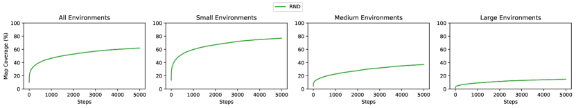
Figure 10: Growth in agent-explored map region as a function of the number of steps from the first step in the environment matches the performance of RND. Mean spatial map coverage performance as a function of the number of steps taken in various sizes of environment sets. The shade denotes the standard error.

References

- [1] Adrià Puigdomènech Badia, Pablo Sprechmann, Alex Vitvitskyi, Daniel Guo, Bilal Piot, Steven Kapturowski, Olivier Tieleman, Martín Arjovsky, Alexander Pritzel, and Andew Bolt. Never give up: Learning directed exploration strategies, 2020.
- [2] Christopher Baldassano, Janice Chen, Asieh Zadbood, Jonathan W Pillow, Uri Hasson, and Kenneth A Norman. Discovering event structure in continuous narrative perception and memory. Neuron, 95(3):709–721, 2017.
- [3] David Ball, Scott Heath, Janet Wiles, Gordon Wyeth, Peter Corke, and Michael Milford. Openratslam: an open source brain-based slam system. Autonomous Robots, 34:149–176, 2013.
- [4] Yuri Burda, Harrison Edwards, Amos Storkey, and Oleg Klimov. Exploration by random network distillation. In ICLR, 2019.
- [5] Francis Carpenter, Daniel Manson, Kate Jeffery, Neil Burgess, and Caswell Barry. Grid cells form a global representation of connected environments. Current Biology, 25(9):1176–1182, 2015.
- [6] Devendra Singh Chaplot, Dhiraj Gandhi, Saurabh Gupta, Abhinav Gupta, and Ruslan Salakhutdinov. Learning to explore using active neural slam. In ICLR, 2020.
- [7] Howie Choset and Keiji Nagatani. Topological simultaneous localization and mapping (slam): toward exact localization without explicit localization. TRA, 17(2):125–137, 2001.
- [8] Laura Lee Colgin, Edvard I Moser, and May-Britt Moser. Understanding memory through hippocampal remapping. Trends in neurosciences, 31(9):469–477, 2008.
- [9] Anna Dai, Sotiris Papatheodorou, Nils Funk, Dimos Tzoumanikas, and Stefan Leutenegger. Fast frontier-based information-driven autonomous exploration with an mav. ICRA, 2020.
- [10] Adrianus Dingeman De Groot. Het denken van den schaker, een experimenteelpsychologie studie. 1946.
- [11] Dori Derdikman, Jonathan R Whitlock, Albert Tsao, Marianne Fyhn, Torkel Hafting, May-Britt Moser, and Edvard I Moser. Fragmentation of grid cell maps in a multicompartment environment. Nature Neuroscience, 12(10):1325–1332, 2009.
- [12] Christian Dornhege and Alexander Kleiner. A frontier-void-based approach for autonomous exploration in 3d. In SSRR, pages 351–356, 2011.
- [13] Dennis E Egan and Barry J Schwartz. Chunking in recall of symbolic drawings. Memory & cognition, 7(2):149–158, 1979.
- [14] Austin Eliazar and Ronald Parr. Dp-slam: Fast, robust simultaneous localization and mapping without predetermined landmarks. In IJCAI, 2003.
- [15] Melih Erdogan. Dataset-of-Gazebo-Worlds-Models-and-Maps. GitHub, 2019.
- [16] Martin Ester, Hans-Peter Kriegel, Jörg Sander, Xiaowei Xu, et al. A density-based algorithm for discovering clusters in large spatial databases with noise. In KDD, 1996.
- [17] Youssef Ezzyat and Lila Davachi. What constitutes an episode in episodic memory? Psychological science, 22(2):243–252, 2011.
- [18] Nathaniel Fairfield, David Wettergreen, and George Kantor. Segmented slam in three-dimensional environments. Journal of Field Robotics, 27(1):85–103, 2010.
- [19] Meire Fortunato, Melissa Tan, Ryan Faulkner, Steven Hansen, Adrià Puigdomènech Badia, Gavin Buttimore, Charles Deck, Joel Z Leibo, and Charles Blundell. Generalization of reinforcement learners with working and episodic memory. In NeurIPS, 2019.
- [20] Marianne Fyhn, Torkel Hafting, Alessandro Treves, May-Britt Moser, and Edvard I Moser. Hippocampal remapping and grid realignment in entorhinal cortex. Nature, 446(7132):190–194, 2007.
- [21] Fernand Gobet, Peter CR Lane, Steve Croker, Peter CH Cheng, Gary Jones, Iain Oliver, and Julian M Pine. Chunking mechanisms in human learning. Trends in cognitive sciences, 5(6):236–243, 2001.
- [22] Fernand Gobet and Herbert A Simon. Expert chess memory: Revisiting the chunking hypothesis. Memory, 6(3):225–255, 1998.
- [23] Giorgio Grisetti, Rainer Kümmerle, Cyrill Stachniss, and Wolfram Burgard. A tutorial on graph-based slam. IEEE Intelligent Transportation Systems Magazine, 2(4):31–43, 2010.
- [24] Torkel Hafting, Marianne Fyhn, Sturla Molden, May-Britt Moser, and Edvard I Moser. Microstructure of a spatial map in the entorhinal cortex. Nature, 436(7052):801–806, 2005.
- [25] Peter E Hart, Nils J Nilsson, and Bertram Raphael. A formal basis for the heuristic determination of minimum cost paths. IEEE transactions on Systems Science and Cybernetics, 4(2):100–107, 1968.
- [26] Sepp Hochreiter and Jürgen Schmidhuber. Long short-term memory. Neural computation, 9(8):1735–1780, 1997.
- [27] Dirk Holz, Nicola Basilico, Francesco Amigoni, and Sven Behnke. Evaluating the efficiency of frontier-based exploration strategies. In ISR, pages 1–8, 2010.
- [28] Chia-Chun Hung, Timothy Lillicrap, Josh Abramson, Yan Wu, Mehdi Mirza, Federico Carnevale, Arun Ahuja, and Greg Wayne. Optimizing agent behavior over long time scales by transporting value. Nature communications, 10(1):5223, 2019.
- [29] Mirko Klukas, Sugandha Sharma, YiLun Du, Tomas Lozano-Perez, Leslie Kaelbling, and Ila Fiete. Fragmented spatial maps from surprisal: state abstraction and efficient planning. bioRxiv, 2021.
- [30] Mihir Kulkarni, Mihir Dharmadhikari, Marco Tranzatto, Samuel Zimmermann, Victor Reijgwart, Paolo De Petris, Huan Nguyen, Nikhil Khedekar, Christos Papachristos, Lionel Ott, et al. Autonomous teamed exploration of subterranean environments using legged and aerial robots. In ICRA, 2022.
- [31] Andrew Lampinen, Stephanie Chan, Andrea Banino, and Felix Hill. Towards mental time travel: a hierarchical memory for reinforcement learning agents. NeurIPS, 2021.
- [32] Steven M LaValle. Rapidly-exploring random trees: A new tool for path planning. 1998.
- [33] Isabel IC Low, Alex H Williams, Malcolm G Campbell, Scott W Linderman, and Lisa M Giocomo. Dynamic and reversible remapping of network representations in an unchanging environment. Neuron, 109(18):2967–2980, 2021.
- [34] Steven Macenski, Tully Foote, Brian Gerkey, Chris Lalancette, and William Woodall. Robot operating system 2: Design, architecture, and uses in the wild. Science Robotics, 7(66), 2022.
- [35] Renan Maffei, Vitor Jorge, Mariana Kolberg, and Edson Prestes. Segmented dp-slam. In IROS, 2013.
- [36] Michael J Milford, Janet Wiles, and Gordon F Wyeth. Solving navigational uncertainty using grid cells on robots. PLoS computational biology, 6(11), 2010.
- [37] Michael J Milford, Gordon F Wyeth, and David Prasser. Ratslam: a hippocampal model for simultaneous localization and mapping. In ICRA, 2004.
- [38] Darren Newtson and Gretchen Engquist. The perceptual organization of ongoing behavior. Journal of Experimental Social Psychology, 12(5):436–450, 1976.
- [39] Alexander Pritzel, Benigno Uria, Sriram Srinivasan, Adria Puigdomenech Badia, Oriol Vinyals, Demis Hassabis, Daan Wierstra, and Charles Blundell. Neural episodic control. In ICML, 2017.
- [40] Lauren L Richmond and Jeffrey M Zacks. Constructing experience: Event models from perception to action. Trends in cognitive sciences, 21(12):962–980, 2017.
- [41] Samuel Ritter, Jane Wang, Zeb Kurth-Nelson, Siddhant Jayakumar, Charles Blundell, Razvan Pascanu, and Matthew Botvinick. Been there, done that: Meta-learning with episodic recall. In ICML, 2018.
- [42] Samuel Ritter, Jane X Wang, Zeb Kurth-Nelson, and Matthew Botvinick. Episodic control as meta-reinforcement learning. BioRxiv, page 360537, 2018.
- [43] Alexei Samsonovich and Bruce L McNaughton. Path integration and cognitive mapping in a continuous attractor neural network model. Journal of Neuroscience, 17(15):5900–5920, 1997.
- [44] John Schulman, Filip Wolski, Prafulla Dhariwal, Alec Radford, and Oleg Klimov. Proximal policy optimization algorithms. arXiv preprint arXiv:1707.06347, 2017.
- [45] Bokui Shen, Fei Xia, Chengshu Li, Roberto Martín-Martín, Linxi Fan, Guanzhi Wang, Claudia Pérez-D’Arpino, Shyamal Buch, Sanjana Srivastava, Lyne Tchapmi, et al. igibson 1.0: A simulation environment for interactive tasks in large realistic scenes. In IROS, 2021.
- [46] Herbert A Simon. How big is a chunk? by combining data from several experiments, a basic human memory unit can be identified and measured. Science, 183(4124):482–488, 1974.
- [47] C. Stachniss, D. Hahnel, and W. Burgard. Exploration with active loop-closing for fastslam. In IROS, 2004.
- [48] Khena M Swallow, Jeffrey M Zacks, and Richard A Abrams. Event boundaries in perception affect memory encoding and updating. Journal of Experimental Psychology: General, 138(2):236, 2009.
- [49] Andrew Szot, Alex Clegg, Eric Undersander, Erik Wijmans, Yili Zhao, John Turner, Noah Maestre, Mustafa Mukadam, Devendra Chaplot, Oleksandr Maksymets, Aaron Gokaslan, Vladimir Vondrus, Sameer Dharur, Franziska Meier, Wojciech Galuba, Angel Chang, Zsolt Kira, Vladlen Koltun, Jitendra Malik, Manolis Savva, and Dhruv Batra. Habitat 2.0: Training home assistants to rearrange their habitat. In NeurIPS, 2021.
- [50] Ashish Vaswani, Noam Shazeer, Niki Parmar, Jakob Uszkoreit, Llion Jones, Aidan N Gomez, Łukasz Kaiser, and Illia Polosukhin. Attention is all you need. NeurIPS, 2017.
- [51] Brian Yamauchi. A frontier-based approach for autonomous exploration. In CIRA, 1997.
- [52] Fan Yang, Dung-Han Lee, John Keller, and Sebastian Scherer. Graph-based topological exploration planning in large-scale 3d environments. In ICRA, 2021.
- [53] Fangwen Yu, Jianga Shang, Youjian Hu, and Michael Milford. Neuroslam: a brain-inspired slam system for 3d environments. Biological cybernetics, 113:515–545, 2019.
- [54] Jeffrey M Zacks and Khena M Swallow. Event segmentation. Current directions in psychological science, 16(2):80–84, 2007.
- [55] Shaowu Zhang, Fiola Bock, Aung Si, Juergen Tautz, and Mandyam V Srinivasan. Visual working memory in decision making by honey bees. PNAS, 102(14):5250–5255, 2005.
- [56] Yukun Zhang, Mengyuan Chen, Dehong Tian, and Lingmei Ding. Biomimetic slam algorithm based on growing self-organizing map. IEEE Access, 9:134660–134671, 2021.