Making the Nyström method highly accurate
for low-rank approximations

Abstract

The Nyström method is a convenient heuristic method to obtain low-rank approximations to kernel matrices in nearly linear complexity. Existing studies typically use the method to approximate positive semidefinite matrices with low or modest accuracies. In this work, we propose a series of heuristic strategies to make the Nyström method reach high accuracies for nonsymmetric and/or rectangular matrices. The resulting methods (called high-accuracy Nyström methods) treat the Nyström method and a skinny rank-revealing factorization as a fast pivoting strategy in a progressive alternating direction refinement process. Two refinement mechanisms are used: alternating the row and column pivoting starting from a small set of randomly chosen columns, and adaptively increasing the number of samples until a desired rank or accuracy is reached. A fast subset update strategy based on the progressive sampling of Schur complements is further proposed to accelerate the refinement process. Efficient randomized accuracy control is also provided. Relevant accuracy and singular value analysis is given to support some of the heuristics. Extensive tests with various kernel functions and data sets show how the methods can quickly reach prespecified high accuracies in practice, sometimes with quality close to SVDs, using only small numbers of progressive sampling steps.

Jianlin XiaHigh-accuracy Nyström methods

15A23, 65F10, 65F30

1 Introduction

The Nyström method is a very useful technique for data analysis and machine learning. It can be used to quickly produce low-rank approximations to data matrices. The original Nyström method in [35] is designed for symmetric positive definite kernel matrices and it essentially uses uniform sampling to select rows/columns (that correspond to some subsets of data points) to serve as basis matrices in low-rank approximations. It has been empirically shown to work reasonably well in practice. The Nyström method is highly efficient in the sense that it can produce a low-rank approximation in complexity linear in the matrix size $n$ (supposing the target approximation rank $r$ is small).

For problems with high coherence [13, 32], the accuracy of the usual Nyström method with uniform sampling may be very low. There have been lots of efforts to improve the method. See, e.g., [10, 13, 22, 42]. In order to gain good accuracy, significant extra costs are needed to estimate leverage scores or determine sampling probabilities in nonuniform sampling [8, 11, 21].

Due to its modest accuracy, the Nyström method is usually used for data analysis and not much for regular numerical computations. In numerical analysis and scientific computing where controllable high accuracies are desired, often truncated SVDs or more practical variations like rank-revealing factorizations [6, 17] and randomized SVD/sketching methods [19, 33] are used. These methods can produce highly reliable low-rank approximations but usually cost $O(n^{2})$ operations.

The purpose of this work is to propose a set of strategies based on the Nyström method to produce high-accuracy low-rank approximations for kernel matrices in about linear complexity. The matrices are allowed to be nonsymmetric and/or rectangular. Examples include off-diagonal blocks of larger kernel matrices that frequently arise from numerical solutions of differential and integral equations, structured eigenvalue solutions, N-body simulations, and image processing. There has been a rich history in studying the low-rank structure of these off-diagonal kernel matrices based on ideas from the fast multipole method (FMM) [15] and hierarchical matrix methods [18]. To obtain a low-rank approximation to such a rectangular kernel matrix $A$ with the Nyström method, a basic way is to choose respectively random row and column index sets $\mathcal{I}$ and $\mathcal{J}$ and then get a so-called CUR approximation

(1) $$A\approx A_{:,\mathcal{J}}A_{\mathcal{I},\mathcal{J}}^{+}A_{\mathcal{I},:},$$

where $A_{:,\mathcal{J}}$ and $A_{\mathcal{I},:}$ denote submatrices formed by the columns and rows of $A$ corresponding to the index sets $\mathcal{J}$ and $\mathcal{I}$, respectively, and $A_{\mathcal{I},\mathcal{J}}$ can be understood similarly. However, the accuracy of (1) is typically low, unless the so-called volume of $A_{\mathcal{I},\mathcal{J}}$ happens to be sufficiently large [14]. It is well known that finding a submatrix with the maximum volume is NP-hard.

Here, we would like to design adaptive Nyström schemes that can produce controllable errors (including near machine precision) while still retaining nearly linear complexity in practice. We start by treating the combination of the Nyström method and a reliable algebraic rank-revealing factorization as a fast pivoting strategy to select significant rows/columns (called representative rows/columns as in [37]). We then provide one way to analyze the resulting low-rank approximation error, which serves as a motivation for the design of our new schemes. Further key strategies include the following.

1. Use selected columns and rows to perform fast alternating direction row and column pivoting, respectively, so as to refine selections of representative rows and columns.

2. Adaptively attach a small number of new samples so as to perform progressive alternating direction pivoting, which produces new expanded representative rows and columns and advances the numerical rank needed to reach high accuracies.

3. Use a fast subset update strategy that successively samples the Schur complements so as to improve the efficiency and accelerate the advancement of the sizes of basis matrix toward target numerical ranks.

4. Adaptively control the accuracy via quick estimation of the approximation errors.

Specifically, in the first strategy above, randomly selected columns are used to quickly perform row pivoting for $A$ and obtain representative rows (which form a row skeleton $A_{\mathcal{I},:}$). The row skeleton is further used to quickly perform column pivoting for $A$ to obtain some representative columns (which form a column skeleton $A_{:,\mathcal{J}}$). This refines the original choice of representative columns. Related methods include various forms of the adaptive cross approximation (ACA) with row/column pivoting [4, 24], the volume sampling approximation [8], and the iterative cross approximation [23]. In particular, the method in [23] iteratively refines selections of significant submatrices (with volumes as large as possible). However, later we can see that this strategy alone is not enough to reach high accuracy, even if a large number of initial samples is used.

Next in the second strategy, new column samples are attached progressively in small stepsizes so as to repeat the alternating direction pivoting until convergence is reached. Convenient uniform sampling is used since the sampled columns are for the purpose of pivoting. This eliminates the need of estimating sampling probabilities. The third strategy enables to avoid applying pivoting to row/column skeletons with growing sizes. That is, the row (column) skeleton is expanded by quickly updating the previous skeleton when new columns (rows) are attached. We also give an aggressive subset update method that can quickly reach high accuracies with a small number of progressive sampling steps in practice. With the forth strategy, we can conveniently control the number of sampling steps until a desired accuracy is reached. It avoids the need to perform quadratic cost error estimation.

The combination of these strategies leads to a type of low-rank approximation schemes which we call high-accuracy Nyström (HAN) schemes. They are heuristic schemes that are both fast and accurate in practice. Although a fully rigorous justification of the accuracy is lacking, we give different perspectives to motivate and support the ideas. Relevant analysis is provided to understand certain singular value and accuracy behaviors in terms of both deterministic rank-revealing factorizations and statistical error evaluation.

We demonstrate the high accuracy of the HAN schemes through comprehensive numerical tests based on kernel matrices defined from various kernel functions evaluated at different data sets. In particular, an aggressive HAN scheme can produce approximation accuracies close to the quality of truncated SVDs. It is numerically shown to have nearly linear complexity and further usually needs just a surprisingly small number of sampling steps.

Additionally, the design of the HAN schemes does not require analytical information from the kernel functions or geometric information from the data points. They can then serve as fully blackbox fast low-rank approximation methods, as indicated in the tests.

The remaining discussions are organized as follows. We show the pivoting strategy based on the Nyström method and give a way to study the approximation error in Section 2. The detailed design of the HAN schemes together with relevant analysis is given in Section 3. Section 4 presents the numerical tests, followed by some concluding remarks in Section 5.

2 Pivoting based on the Nyström method and an error study

We first consider a low-rank approximation method based on a pivoting strategy consisting of the Nyström method and rank-revealing factorizations of tall and skinny matrices. A way to study the low-rank approximation error will then be given. These will provide motivations for some of our ideas in the HAN schemes.

Consider two sets of real data points in $d$ dimensions:

$$\mathbf{x}=\left\{x_{1},x_{2},\ldots,x_{m}\right\},\quad\mathbf{y}=\left\{y_{1},y_{2},\ldots,y_{n}\right\}.$$

Let $A$ be the $m\times n$ kernel matrix

(2) $$A=\left(\kappa(x_{i},y_{j})\right)_{x_{i}\in\mathbf{x},y_{j}\in\mathbf{y}},$$

which is sometimes also referred to as the interaction matrix between $\mathbf{x}$ and $\mathbf{y}$. We would like to approximate $A$ by a low-rank form. The strong rank-revealing QR or LU factorizations [17, 26] are reliable ways to find low-rank approximations with high accuracy. They may be used to obtain an approximation (called interpolative decomposition) of the following form:

(3) $$A\approx A_{:,\mathcal{J}}V^{T}\quad\text{with\quad}V=Q\left(\begin{array}[c]{c}I\\ F\end{array}\right),$$

where $Q$ is a permutation matrix, $r\equiv|\mathcal{J}|$ (size or cardinality of $\mathcal{J}$) is the approximate (or numerical) rank, and $\|F\|_{\max}\leq c$ with $c\geq 1$. $c$ is a user-specified parameter and may be set to be a constant or a low-degree polynomial of $m$, $n$, and $r$ [17].

We suppose $r$ is small. The column skeleton $A_{:,\mathcal{J}}$ corresponds to a subset $\mathbf{t}\subset\mathbf{y}$ which is a subset of landmark points. Here we also call $\mathbf{t}$ a representative subset, which can be selected reliably by strong rank-revealing factorizations. A strong rank-revealing factorization may be further applied to $A_{:,\mathcal{J}}^{T}$ to select a representative subset $\mathbf{s}\subset\mathbf{x}$ corresponding to a row index set $\mathcal{I}$ in $A_{:,\mathcal{J}}$. That is, we can find a pivot block $A_{\mathcal{I},\mathcal{J}}$. Without loss of generality, we may assume $|\mathcal{I}|=|\mathcal{J}|=r$. (If the factorization produces $\mathcal{I}$ with $|\mathcal{I}|<|\mathcal{J}|$, $V$ can be modified so as to replace $\mathcal{J}$ by an appropriate index set with size $|\mathcal{I}|$.) Thus, the resulting decomposition may be written as an equality

(4) $$A_{:,\mathcal{J}}=UA_{\mathcal{I},\mathcal{J}}\quad\text{with\quad}U=P\left(\begin{array}[c]{c}I\\ E\end{array}\right),$$

where $P$ is a permutation matrix and, with $1:m$ standing for $1,2,\ldots,m$,

(5) $$E=A_{\{1:m\}\backslash\mathcal{I},\mathcal{J}}A_{\mathcal{I},\mathcal{J}}^{-1},\quad\|E\|_{\max}\leq c.$$

Since $A_{:,\mathcal{J}}$ is a tall and skinny matrix, we refer to (4) as a skinny rank-revealing (SRR) factorization. (3) and (4) in turn lead to the approximation

(6) $$A\approx UA_{\mathcal{I},\mathcal{J}}V^{T}.$$

With (6), we may further obtain a CUR approximation like in (1) (with the pseudoinverse replaced by $A_{\mathcal{I},\mathcal{J}}^{-1}$).

The direct application of strong rank-revealing factorizations to $A$ to obtain (3) is expensive and costs $O(rmn)$. To reduce the cost, we can instead follow the Nyström method and randomly sample columns from $A$ to form $A_{:,\mathcal{J}}$. However, the accuracy of the resulting approximation based on the forms (3) or (6) may be low. On the other hand, we can view the SRR factorization (4) as a way to quickly choose the representative subset $\mathbf{s}$ (based on the interaction between $\mathbf{x}$ and $\mathbf{t}$ instead of the interaction between $\mathbf{x}$ and $\mathbf{y}$). In other words, (4) is a way to quickly perform row pivoting for $A$ so as to select representative rows $A_{\mathcal{I},:}$ from $A$. Then we can use the following low-rank approximation:

(7) $$A\approx UA_{\mathcal{I},:}\quad\text{with\quad}U=P\left(\begin{array}[c]{c}I\\ E\end{array}\right),$$

which may be viewed as a potentially refined form over (3) when $\mathcal{J}$ is randomly selected. (Note that $P$ and $E$ depend on $\mathcal{J}$.)

We would like to gain some insights into the accuracy of approximations based on the Nyström method. There are various earlier studies based on (1). Those in [5, 42] are relevant to our result below. When $A$ is positive (semi-)definite, the analysis in [42] bounds the errors in terms of the distances between the landmark points and the remaining data points. A similar strategy is also followed in [5, Lemma 3.1] for symmetric $A$. The resulting bound may be very conservative since it is common for some data points in practical data sets to be far away from the landmark points. In addition, the error bounds in [5, 42] essentially involve a factor $\|A_{\mathcal{I},\mathcal{J}}^{-1}\|_{2}$ (or $\|A_{\mathcal{I},\mathcal{J}}^{+}\|_{2}$), which may be too large if high accuracy is desired. This is because the smallest singular value of $A_{11}$ may be just slightly larger than a smaller tolerance.

Here, we provide a way to understand the approximation error based on (7). It uses the minimization of a slightly overdetermined problem and does not involve $\|A_{\mathcal{I},\mathcal{J}}^{-1}\|_{2}$. The following analysis does not aim to precisely quantify the error magnitude (which is hard anyway). Instead, it can serve as a motivation for some strategies in our high-accuracy Nyström methods later.

Lemma 2.1.

Suppose $\mathcal{J}$ is a given column index set with $|\mathcal{J}|=r$ and (4)–(5) hold. Then the resulting approximation (7) satisfies

(8) $$\|A-UA_{\mathcal{I},:}\|_{\max}\leq 2c\sqrt{r}\max_{1\leq i\leq m,1\leq j\leq n}\min_{v\in\mathbb{R}^{r}}\|A_{\widetilde{\mathcal{I}}_{i},\mathcal{J}}v-A_{\widetilde{\mathcal{I}}_{i},j}\|_{2},$$

where $\widetilde{\mathcal{I}}_{i}=\mathcal{I}\cup\{i\}$ for each $1\leq i\leq m$.

Proof 2.2.

From (4) and (7), we have, for any $1\leq i\leq m$, $1\leq j\leq n$,

$$(A-UA_{\mathcal{I},:})_{ij}=(A-A_{:,\mathcal{J}}A_{\mathcal{I},\mathcal{J}}^{-1}A_{\mathcal{I},:})_{ij}=A_{ij}-A_{i,\mathcal{J}}A_{\mathcal{I},\mathcal{J}}^{-1}A_{\mathcal{I},j}.$$

It is obvious that $A_{ij}-A_{i,\mathcal{J}}A_{\mathcal{I},\mathcal{J}}^{-1}A_{\mathcal{I},j}=0$ if $i\in\mathcal{I}$. Thus, suppose $i\in\{1:m\}\backslash\mathcal{I}$.

For any $v\in\mathbb{R}^{r}$,

$$|A_{ij}-A_{i,\mathcal{J}}A_{\mathcal{I},\mathcal{J}}^{-1}A_{\mathcal{I},j}| =|(A_{ij}-A_{i,\mathcal{J}}v)+(A_{i,\mathcal{J}}v-A_{i,\mathcal{J}}A_{\mathcal{I},\mathcal{J}}^{-1}A_{\mathcal{I},j})|$$

$$\leq|A_{ij}-A_{i,\mathcal{J}}v|+\|A_{i,\mathcal{J}}A_{\mathcal{I},\mathcal{J}}^{-1}\|_{2}\|A_{\mathcal{I},\mathcal{J}}v-A_{\mathcal{I},j}\|_{2}$$

$$\leq|A_{ij}-A_{i,\mathcal{J}}v|+c\sqrt{r}\|A_{\mathcal{I},\mathcal{J}}v-A_{\mathcal{I},j}\|_{2},$$

where the last step is because $A_{i,\mathcal{J}}A_{\mathcal{I},\mathcal{J}}^{-1}$ is a row of $E$ in (5) and its entries have magnitudes bounded by $c$. With $c\geq 1$, we further have

$$|A_{ij}-A_{i,\mathcal{J}}A_{\mathcal{I},\mathcal{J}}^{-1}A_{\mathcal{I},j}| \leq c\sqrt{r}\left(|A_{i,\mathcal{J}}v-A_{ij}|+\|A_{\mathcal{I},\mathcal{J}}v-A_{\mathcal{I},j}\|_{2}\right)$$

$$\leq 2c\sqrt{r}\|A_{\widetilde{\mathcal{I}}_{i},\mathcal{J}}v-A_{\widetilde{\mathcal{I}}_{i},j}\|_{2}.$$

Since this holds for all $v\in\mathbb{R}^{r}$, take the minimum for $v$ to get the desired result.

The bound in this lemma can be roughly understood as follows. If $A_{\widetilde{\mathcal{I}}_{i},j}$ is nearly in the range of $A_{\widetilde{\mathcal{I}}_{i},\mathcal{J}}$ for all $i,j$, the bound in (8) would then be very small and we would have found $\mathcal{I}$ and $\mathcal{J}$ that produce an accurate low-rank approximation (7). Otherwise, to further improve the accuracy, it would be necessary to refine $\mathcal{I}$ and $\mathcal{J}$ and possibly include additional $i$ and $j$ indices respectively into $\mathcal{I}$ and $\mathcal{J}$. A heuristic strategy is to progressively pick $i$ and $j$ so that $A_{\widetilde{\mathcal{I}}_{i},j}$ is as linearly independent from the columns of $A_{\widetilde{\mathcal{I}}_{i},\mathcal{J}}$ as possible. Motivated by this, we may use a subset refinement process. First, use randomly picked columns $A_{:,\mathcal{J}}$ to generate a row skeleton and then use the row skeleton to generate a new column skeleton. The new column skeleton suggests which new $j$ should be attached to $\mathcal{J}$. Next, if a desired accuracy is not reached, then randomly pick more columns to attach to the refined set $\mathcal{J}$ and start a new round of refinement. Such a process is called progressive alternating direction pivoting (or subset refinement) below.

3 High-accuracy Nyström schemes

In this section, we show how to use the Nyström method to design the high-accuracy Nyström (HAN) schemes that can produce highly accurate low-rank approximations in practice. We begin with the basic idea of the progressive alternating direction pivoting and then show how to perform fast subset update and how to conveniently control the accuracy.

3.1 Progressive alternating direction pivoting

The direct application of strong rank-revealing factorizations to $A$ has quadratic complexity. One way to save the cost is as follows. Start from some column samples of $A$ like in the usual Nyström method. Use the SRR factorization to select a row skeleton, which can then be used to select a refined column skeleton. The process can be repeated in a recursive way, leading to a fast alternating direction refinement scheme. A similar empirical scheme has been adopted recently in [23, 29]. However, when high accuracies are desired, the effectiveness of this scheme may be limited. That is, just like the usual Nyström method, a brute-force increase of the initial sample size may not necessarily improve the approximation accuracy significantly. A high accuracy may require the initial sample size to be overwhelmingly larger than the target numerical rank, which makes the cost too high.

Here, we instead adaptively or progressively apply the alternating direction refinement based on step-by-step small increases of the sample size. We use one round of alternating row and column pivoting to refine the subset selections. After this, if a target accuracy $\tau$ or numerical rank $r$ is not reached, we include a small number of additional samples to repeat the procedure.

The basic framework to find a low-rank approximation to $A$ in (2) is as follows, where the subset $\mathcal{J}$ is initially an empty set and $b\leq r$ is a small integer as the stepsize in the progressive column sampling.

1. (Progressive sampling) Randomly choose a column index set $\widehat{\mathcal{J}}\subset\{1:n\}\backslash\mathcal{J}$ with $|\widehat{\mathcal{J}}|=b$ and set

   $$\widetilde{\mathcal{J}}=\mathcal{J}\cup\widehat{\mathcal{J}}.$$

2. (Row pivoting) Apply an SRR factorization to $A_{:,\widetilde{\mathcal{J}}}$ to find a row index set $\mathcal{I}$:

   (9) $$A_{:,\widetilde{\mathcal{J}}}\approx UA_{\mathcal{I},\widetilde{\mathcal{J}}},$$

   where $U$ looks like that in (4).

3. (Column pivoting) Apply an SRR factorization to $A_{\mathcal{I},:}$ to find a refined column index set $\mathcal{J}$:

   (10) $$A_{\mathcal{I},:}\approx A_{\mathcal{I},\mathcal{J}}V^{T},$$

   where $V$ looks like that in (3).

4. (Accuracy check) If a desired accuracy, maximum sample size, or a target numerical rank is reached or if $\mathcal{I}$ stays the same as in the previous step, return a low-rank approximation to $A$ like the following and exit:

   $$\tilde{A}=UA_{\mathcal{I},:},\quad A_{:,\mathcal{J}}V^{T},\quad\text{or\quad}UA_{\mathcal{I},\mathcal{J}}V^{T}.$$

   Otherwise, repeat from Step 1. (More details on the stopping criteria and fast error estimation will be given in Section 3.3.)

This basic HAN scheme (denoted HAN-B) is illustrated in Figure 1, with more details given in Algorithm 1. Note that the key outputs of the SRR factorization (4) are the index set $\mathcal{I}$ and the matrix $E$. (The permutation matrix $P$ is just to bring the index set $\mathcal{I}$ to the leading part and does not need to be stored.) For convenience, we denote (4) by the following procedure in Algorithm 1 (with the parameter $c$ in (5) assumed to be fixed):

$$[\mathcal{I},E]\leftarrow\mathsf{SRR}(A_{:,\mathcal{J}}).$$

The scheme may be understood heuristically as follows. Initially, with $\widetilde{\mathcal{J}}$ a random sample from the column indices, it is known that the expectation of the norm of a row of $A_{:,\widetilde{\mathcal{J}}}$ is a multiple of the norm of the corresponding row in $A$ (see, e.g., [1, 9]). Thus, the relative magnitudes of the row norms of $A$ can be roughly reflected by those of $A_{:,\widetilde{\mathcal{J}}}$. It then makes sense to use $A_{:,\widetilde{\mathcal{J}}}$ for quick row pivoting (by finding $A_{\mathcal{I},\widetilde{\mathcal{J}}}$ with determinant as large as possible). This strategy shares features similar to the randomized pivoting strategies in [25, 40] which are also heuristic and work well in practice, except that the methods in [25, 40] need matrix-vector multiplications with costs $O(mn)$.

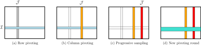
Figure 1: Illustration of the basic high-accuracy Nyström (HAN-B) scheme.

Algorithm 1 Basic HAN scheme

1:procedure HAN-B($A$, $b$, $\tau$ (or $r$))

2:     $\mathcal{J}\leftarrow\varnothing$

3:     for $i=1,2,\ldots$ do

4:         $\widehat{\mathcal{J}}\leftarrow$ randomly chosen index set from $\{1:n\}\backslash\mathcal{J}$ with $|\widehat{\mathcal{J}}|=b$

5:         $\widetilde{\mathcal{J}}\leftarrow\mathcal{J}\cup\widehat{\mathcal{J}}$$\triangleright$ Progressive sampling

6:         $\overline{\mathcal{I}}\leftarrow\mathcal{I}$

7:         $[\mathcal{I},E]\leftarrow$ SRR$(A_{:,\widetilde{\mathcal{J}}})$$\triangleright$ Row pivoting

8:         $\widehat{\mathcal{I}}\leftarrow\mathcal{I}\backslash\overline{\mathcal{I}}$$\triangleright$ Removal of indices in the previous $\mathcal{I}$ from the new one

9:         $[\mathcal{J},F]\leftarrow$ SRR$(A_{\mathcal{I},:}^{T})$$\triangleright$ Column pivoting

10:         if a target accuracy $\tau$ or numerical rank $r$ is reached or $\widehat{\mathcal{I}}=\varnothing$ then $\triangleright$ See Section 3.3 for more discussions

11:              Return $A\approx UA_{\mathcal{I},:}$, $A_{:,\mathcal{J}}V^{T}$, or $UA_{\mathcal{I},\mathcal{J}}V^{T}$

12:         end if

13:     end for

14:end procedure

With the resulting row pivot index set $\mathcal{I}$, the scheme further uses the SRR factorization to find a submatrix $A_{\mathcal{I},\mathcal{J}}$ of $A_{\mathcal{I},:}$ with determinant as large as possible, which enables to refine the column selection. It may be possible to further improve the index sets through multiple rounds of such refinements like in [23, 29]. However, the accuracy gain seems limited, even if a large initial sample size is used (as shown in our test later). Thus, we progressively attach additional samples (in small stepsizes) to the refined subset $\mathcal{J}$ and then repeat the previous procedure. In practice, this makes a significant difference in reducing the approximation error.

In this scheme, the sizes of the index sets $\mathcal{I}$ and $\mathcal{J}$ grow with the progressive sampling. Accordingly, the costs of the SRR factorizations (9)–(10) increase since the SRR factorizations at step $i$ are applied to matrices of sizes $m\times(ib)$ or $(ib)\times n$. With the total number of iterations $N\approx\frac{r}{b}$, the total cost (excluding the cost to check the accuracy) is

(11) $$\xi_{\mathsf{HAN-B}}=\sum_{i=1}^{N}O\left((ib)^{2}(m+n)\right)=O\left(\frac{r^{3}}{b}(m+n)\right).$$

With $i$ increases, the iterations advance toward the target numerical rank or accuracy.

3.2 Fast subset update via Schur complement sampling

In the basic scheme HAN-B, the complexity count in (11) for the SRR factorizations at step $i$ gets higher with increasing $i$. To improve the efficiency, we show how to update the index sets so that at step $i$, the SRR factorization (for the row pivoting step for example) only needs to be applied to a matrix of size $(m-(i-1)b)\times b$ instead of $m\times(ib)$, followed by some quick postprocessing steps.

Suppose we start from a column index set $\widetilde{\mathcal{J}}=\mathcal{J}\cup\widehat{\mathcal{J}}$ as in Step 1 of the basic HAN scheme above. We would like to avoid applying the SRR factorizations to the full columns $A_{:,\widetilde{\mathcal{J}}}$ in Step 2 and the full rows $A_{\mathcal{I},:}$ in Step 3. We seek to directly produce an expanded column index set over $\mathcal{J}$, as illustrated in Figure 2. It includes two steps. One is to produce an update $\widehat{\mathcal{I}}$ to the row index set $\mathcal{I}$ (Figure 2(a), which replaces Steps (c)–(d) in Figure 1) and the other is to produce an update to the column index set (Figure 2(b)). Clearly, we just need to show how to perform the first step.

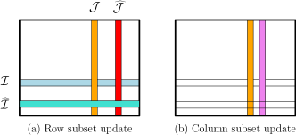
Figure 2: Illustration of the subset update process.

With the row pivoting step like in (9), we can obtain a low-rank approximation of the form (7). Using the row permutation matrix $P$ in (7) (computed in (4)), we may write $A$ as

(17) $$A =P\left(\begin{array}[c]{cc}A_{11}&A_{12}\\ A_{21}&A_{22}\end{array}\right)\approx P\left(\begin{array}[c]{c}I\\ E\end{array}\right)\left(\begin{array}[c]{cc}A_{11}&A_{12}\end{array}\right)\quad\text{with}$$

$$A_{11} =A_{\mathcal{I},\mathcal{J}},\quad E=A_{21}A_{11}^{-1}.$$

At this point, we have

(18) $$A=P\left(\begin{array}[c]{cc}I&\\ E&I\end{array}\right)\left(\begin{array}[c]{cc}A_{11}&A_{12}\\ &S\end{array}\right)\quad\text{with\quad}S=A_{22}-EA_{12},$$

where $S$ is the Schur complement.

Remark 3.1.

In the usual strong rank-revealing factorizations like the one in [26], the low-rank approximation is obtained also from a decomposition of the form (18) with $S$ dropped. Here, our fast pivoting scheme is more efficient. Of course, the strong rank-revealing factorization in [26] guarantees the quality of the low-rank approximation in the sense that, there exist low-degree polynomials $c\geq 1$ and $f\geq 1$ in $m$, $n$, and $k$ (size of $A_{11}$) such that (5) holds and, for $1\leq i\leq k$, $1\leq j\leq\min\{m,n\}-k$,

(19) $$\sigma_{i}(A_{11})\geq\frac{\sigma_{i}(A)}{f},\quad\sigma_{j}(S)\leq\sigma_{k+j}(A)f,\quad\|A_{11}^{-1}A_{12}\|_{\max}\leq c,$$

where $\sigma_{i}(\cdot)$ denotes the $i$-th largest singular value of a matrix.

Our subset update strategy is via the sampling of the Schur complement $S$. In fact, when $A_{\mathcal{I},:}=\left(\begin{array}[c]{cc}A_{11}&A_{12}\end{array}\right)$ is accepted as a reasonable row skeleton, we then continue to find a low-rank approximation to $S$ in (18) so it makes sense to sample $S$. It is worth noting that the full matrix $S$ is not needed. Instead, only its columns corresponding to $A_{:,\widehat{\mathcal{J}}}$ are formed. That is, we form

$$S_{:,\mathcal{L}}=(A_{22})_{:,\mathcal{L}}-E(A_{12})_{:,\mathcal{L}},$$

where $\mathcal{L}$ corresponds to $\widehat{\mathcal{J}}$ and selects entries from $\{1:n\}\backslash\mathcal{J}$ in a two-level composition of the index sets as follows:

(20) $$(\{1:n\}\backslash\mathcal{J})\circ\mathcal{L}=\widehat{\mathcal{J}}.$$

That is, sampling the columns of $A$ with the index set $\widehat{\mathcal{J}}$ is essentially to sample the columns of $S$ with $\mathcal{L}$. For notational convenience, suppose the columns of $A$ have been permuted so that

$$P^{T}A=\left(\begin{array}[c]{c|c}A_{11}&A_{12}\\ A_{21}&A_{22}\end{array}\right)\quad\text{with\quad}A_{:,\mathcal{J}}=\begin{pmatrix}A_{11}\\ A_{21}\end{pmatrix}.$$

Now, apply an SRR factorization to $S_{:,\mathcal{L}}$ to get

(21) $$S_{:,\mathcal{L}}\approx\hat{P}\left(\begin{array}[c]{c}I\\ \hat{E}\end{array}\right)S_{\mathcal{K},\mathcal{L}}.$$

Then $S\approx\hat{P}\left(\begin{array}[c]{c}I\\ \hat{E}\end{array}\right)S_{\mathcal{K},:}$. Accordingly, we may write $S$ as

(22) $$S=\hat{P}\left(\begin{array}[c]{cc}S_{22}&S_{23}\\ S_{32}&S_{33}\end{array}\right),$$

where $S_{\mathcal{K},:}=\left(\begin{array}[c]{cc}S_{22}&S_{23}\end{array}\right)$. From (21) and (22), $S$ can be further written as

(23) $$S=\hat{P}\left(\begin{array}[c]{cc}I&\\ \hat{E}&\hat{S}\end{array}\right)\left(\begin{array}[c]{cc}S_{22}&S_{23}\\ &I\end{array}\right)\quad\text{with\quad}\hat{S}=S_{33}-\hat{E}S_{23},$$

where $\hat{S}$ is a new Schur complement (and is not formed).

At this point, we have the following proposition which shows how to expand the row index set $\mathcal{I}$ by an update $\widehat{\mathcal{I}}$.

Proposition 3.2.

$A$ may be factorized as

(24) $$A=\tilde{P}\left(\begin{array}[c]{cc}I&\\ \tilde{E}&I\end{array}\right)\left(\begin{array}[c]{cc}A_{\widetilde{\mathcal{I}},\widetilde{\mathcal{J}}}&A_{\widetilde{\mathcal{I}},\{1:n\}\backslash\widetilde{\mathcal{J}}}\\ &\hat{S}\end{array}\right),$$

where $\tilde{P}$ is a permutation matrix, $\widetilde{\mathcal{I}}=\mathcal{I}\cup\widehat{\mathcal{I}}$ with

(25) $$\widehat{\mathcal{I}}=(\{1:m\}\backslash\mathcal{I)}\circ\mathcal{K},$$

and $\|\tilde{E}\|_{\max}\leq bc^{2}+c$ when $\|E\|_{\max}\leq c$, $\|\hat{E}\|_{\max}\leq c$, and $|\widehat{\mathcal{J}}|=b$.

Proof 3.3.

(18) and (23) lead to

(30) $$A =P\left(\begin{array}[c]{cc}I&\\ E&I\end{array}\right)\left(\begin{array}[c]{cc}A_{11}&A_{12}\\ &\hat{P}\begin{pmatrix}I&\\ \hat{E}&\hat{S}\end{pmatrix}\begin{pmatrix}S_{22}&S_{23}\\ &I\end{pmatrix}\end{array}\right)$$

(35) $$=P\left(\begin{array}[c]{cc}I&\\ E&\hat{P}\begin{pmatrix}I&\\ \hat{E}&\hat{S}\end{pmatrix}\end{array}\right)\left(\begin{array}[c]{cc}A_{11}&A_{12}\\ &\begin{pmatrix}S_{22}&S_{23}\\ &I\end{pmatrix}\end{array}\right)$$

(42) $$=P\left(\begin{array}[c]{cc}I&\\ &\hat{P}\end{array}\right)\left(\begin{array}[c]{cc}I&\\ \hat{P}^{T}E&\begin{pmatrix}I&\\ \hat{E}&\hat{S}\end{pmatrix}\end{array}\right)\left(\begin{array}[c]{cc}A_{11}&A_{12}\\ &\begin{pmatrix}S_{22}&S_{23}\\ &I\end{pmatrix}\end{array}\right)$$

(49) $$=\tilde{P}\left(\begin{array}[c]{ccc}I&&\\ E_{1}&I&\\ E_{2}&\hat{E}&\hat{S}\end{array}\right)\left(\begin{array}[c]{ccc}A_{11}&\hat{A}_{12}&\hat{A}_{13}\\ &S_{22}&S_{23}\\ &&I\end{array}\right),$$

where $\tilde{P}=P\begin{pmatrix}I&\\ &\hat{P}\end{pmatrix}$, $\hat{P}^{T}E$ is partitioned as $\begin{pmatrix}E_{1}\\ E_{2}\end{pmatrix}$ conformably with $\begin{pmatrix}I\\ \hat{E}\end{pmatrix}$, and $A_{12}$ is partitioned as $\left(\begin{array}[c]{cc}\hat{A}_{12}&\hat{A}_{13}\end{array}\right)$ with $\hat{A}_{12}=A_{\mathcal{I},\widehat{\mathcal{J}}}$.

We can now factorize the second factor on the far right-hand side of (30) as

$$\left(\begin{array}[c]{ccc}I&&\\ E_{1}&I&\\ E_{2}&\hat{E}&\hat{S}\end{array}\right)=\left(\begin{array}[c]{ccc}I&&\\ &I&\\ \bar{E}&\hat{E}&\hat{S}\end{array}\right)\left(\begin{array}[c]{ccc}I&&\\ E_{1}&I&\\ &&I\end{array}\right),$$

where

(50) $$\bar{E}=E_{2}-\hat{E}E_{1}.$$

Then, $A$ may be written as

(60) $$A =\tilde{P}\left(\begin{array}[c]{ccc}I&&\\ &I&\\ \bar{E}&\hat{E}&\hat{S}\end{array}\right)\left(\begin{array}[c]{ccc}I&&\\ E_{1}&I&\\ &&I\end{array}\right)\left(\begin{array}[c]{ccc}A_{11}&\hat{A}_{12}&\hat{A}_{13}\\ &S_{22}&S_{23}\\ &&I\end{array}\right)$$

(67) $$=\tilde{P}\left(\begin{array}[c]{ccc}I&&\\ &I&\\ \bar{E}&\hat{E}&I\end{array}\right)\left(\begin{array}[c]{ccc}A_{11}&\hat{A}_{12}&\hat{A}_{13}\\ \hat{A}_{21}&\hat{A}_{22}&\hat{A}_{23}\\ &&\hat{S}\end{array}\right)$$

where

$$\begin{pmatrix}\hat{A}_{21}&\hat{A}_{22}&\hat{A}_{23}\end{pmatrix}=\begin{pmatrix}0&S_{22}&S_{23}\end{pmatrix}+E_{1}\begin{pmatrix}A_{11}&\hat{A}_{12}&\hat{A}_{13}\end{pmatrix}.$$

The block $\begin{pmatrix}\hat{A}_{21}&\hat{A}_{22}&\hat{A}_{23}\end{pmatrix}$ essentially corresponds to the rows of $A$ with index set $\widehat{\mathcal{I}}$ in (25). This is because of the special form of the second factor on the right-hand side of (60). Then get (24) by letting

$$\tilde{E}=\begin{pmatrix}\bar{E}&\hat{E}\end{pmatrix}.$$

Now since $\|E\|_{\max}\leq c$, $\|\hat{E}\|_{\max}\leq c$, and $\hat{E}$ has column size $b$, we have $\|\bar{E}\|_{\max}\leq bc^{2}+c$. Accordingly, $\|\tilde{E}\|_{\max}\leq bc^{2}+c$.

This proposition shows that we can get a factorization (24) similar to (18), but with the expanded row skeleton $A_{\widetilde{\mathcal{I}},:}$. Accordingly, we may then obtain a new approximation to $A$ similar to (7):

(68) $$A\approx\tilde{U}A_{\widetilde{\mathcal{I}},:}\quad\text{with\quad}\tilde{U}=\tilde{P}\left(\begin{array}[c]{c}I\\ \tilde{E}\end{array}\right),$$

To support the reliability of such an approximation, we can use the following way. As mentioned in Remark 3.1, if (18) is assumed to be obtained by a strong rank-revealing factorization, then we would have nice singular value bounds in (19). Now, if we assume that is the case and (23) is also obtained by a strong rank-revealing factorization, then we would like to show (24) from the subset update would also satisfy some nice singular value bounds. For this purpose, we need the following lemma.

Lemma 3.4.

If (18) is assumed to satisfy (19) with $k=|\mathcal{I}|$ the size of $A_{11}$, and (23) is assumed to satisfy, for $1\leq i\leq b$, $1\leq j\leq\min\{m,n\}-k-b$,

(69) $$\sigma_{i}(S_{22})\geq\frac{\sigma_{i}(S)}{\hat{f}},\quad\sigma_{j}(\hat{S})\leq\sigma_{b+j}(S)\hat{f},$$

where $\hat{f}\geq 1$, then $\mu=\frac{\sigma_{k}(A_{11})}{\sigma_{1}(S_{22})}$ satisfies

$$\frac{1}{f^{2}}\leq\mu\leq s\hat{f},$$

where $s=\frac{\sigma_{k}(A)}{\sigma_{k+1}(A)}$.

Proof 3.5.

By (19) and the interlacing property of singular values,

$$\sigma_{k}(A_{11})\geq\frac{\sigma_{k}(A)}{f},\quad\sigma_{1}(S_{22})\leq\sigma_{1}(S)\leq\sigma_{k+1}(A)f,$$

which yield

$$\mu\geq\frac{\sigma_{k}(A)/f}{\sigma_{k+1}(A)f}\geq\frac{1}{f^{2}}.$$

Similarly, by the interlacing property of singular values and (69),

$$\sigma_{k}(A_{11})\leq\sigma_{k}(A),\quad\sigma_{1}(S_{22})\geq\frac{\sigma_{1}(S)}{\hat{f}}\geq\frac{\sigma_{k+1}(A)}{\hat{f}},$$

where the result $\sigma_{1}(S)\geq\sigma_{k+1}(A)$ directly follows from Weyl’s inequality or [20, Theorem 3.3.16]:

$$\sigma_{k+1}(A) =\sigma_{k+1}\left(P\left(\begin{array}[c]{c}I\\ E\end{array}\right)\left(\begin{array}[c]{cc}A_{11}&A_{12}\end{array}\right)+P\left(\begin{array}[c]{cc}0&\\ &S\end{array}\right)\right)$$

$$\leq\sigma_{k+1}\left(P\left(\begin{array}[c]{c}I\\ E\end{array}\right)\left(\begin{array}[c]{cc}A_{11}&A_{12}\end{array}\right)\right)+\sigma_{1}\left(P\left(\begin{array}[c]{cc}0&\\ &S\end{array}\right)\right)=0+\sigma_{1}(S).$$

Then

$$\mu\leq\frac{\sigma_{k}(A)}{\sigma_{k+1}(A)/\hat{f}}=s\hat{f}.$$

As a quick note, here $s=\frac{\sigma_{k}(A)}{\sigma_{k+1}(A)}$ reflects the gap between $\sigma_{k}(A)$ and $\sigma_{k+1}(A)$. Since we seek to expand the index sets $\mathcal{I}$ and $\mathcal{J}$ (and $k$ hasn’t yet reached the target numerical rank $r$), it is reasonable to regard $s$ as a modest magnitude. Now we are ready to show the singular value bounds.

Proposition 3.6.

With the assumptions and notation in Lemma 3.4, (24) satisfies, for $1\leq i\leq k+b$, $1\leq j\leq\min\{m,n\}-k-b$,

(70) $$\sigma_{i}(A_{\widetilde{\mathcal{I}},\widetilde{\mathcal{J}}})\geq\frac{\sigma_{i}(A)}{\tilde{f}},\quad\sigma_{j}(\hat{S})\leq\sigma_{k+b+j}(A)\tilde{f},$$

where $\tilde{f}=(1+s\hat{f}+s\hat{f}b^{2}c^{2})f^{2}\hat{f}$.

Proof 3.7.

According to (60), $A_{\widetilde{\mathcal{I}},\widetilde{\mathcal{J}}}=\begin{pmatrix}I&\\ E_{1}&I\end{pmatrix}\begin{pmatrix}A_{11}&\hat{A}_{12}\\ &S_{22}\end{pmatrix}$. With a strategy like in [17, 26], rewrite $A_{\widetilde{\mathcal{I}},\widetilde{\mathcal{J}}}$ as

$$A_{\widetilde{\mathcal{I}},\widetilde{\mathcal{J}}}=\begin{pmatrix}I&\\ E_{1}&\frac{1}{\sqrt{\mu}}I\end{pmatrix}\begin{pmatrix}A_{11}&\\ &\mu S_{22}\end{pmatrix}\begin{pmatrix}I&A_{11}^{-1}\hat{A}_{12}\\ &\frac{1}{\sqrt{\mu}}I\end{pmatrix},$$

where $\mu=\frac{\sigma_{k}(A_{11})}{\sigma_{1}(S_{22})}$. Then

$$\begin{pmatrix}A_{11}&\\ &\mu S_{22}\end{pmatrix}=\begin{pmatrix}I&\\ -\sqrt{\mu}E_{1}&\sqrt{\mu}I\end{pmatrix}A_{\widetilde{\mathcal{I}},\widetilde{\mathcal{J}}}\begin{pmatrix}I&-\sqrt{\mu}A_{11}^{-1}\hat{A}_{12}\\ &\sqrt{\mu}I\end{pmatrix}$$

By [20, Theorem 3.3.16],

$$\sigma_{i}\left(\begin{pmatrix}A_{11}&\\ &\mu S_{22}\end{pmatrix}\right) \leq\sigma_{i}(A_{\widetilde{\mathcal{I}},\widetilde{\mathcal{J}}})\left\|\begin{pmatrix}I&\\ -\sqrt{\mu}E_{1}&\sqrt{\mu}I\end{pmatrix}\right\|_{2}\left\|\begin{pmatrix}I&-\sqrt{\mu}A_{11}^{-1}\hat{A}_{12}\\ &\sqrt{\mu}I\end{pmatrix}\right\|_{2}$$

$$\leq\sigma_{i}(A_{\widetilde{\mathcal{I}},\widetilde{\mathcal{J}}})\sqrt{1+\mu+\mu\|E_{1}\|_{2}^{2}}\sqrt{1+\mu+\mu\|A_{11}^{-1}\hat{A}_{12}\|_{2}^{2}}$$

$$\leq\sigma_{i}(A_{\widetilde{\mathcal{I}},\widetilde{\mathcal{J}}})(1+s\hat{f}+s\hat{f}b^{2}c^{2}),$$

where the last inequality is from Lemma 3.4 and the fact that $E_{1}$ and $A_{11}^{-1}\hat{A}_{12}$ are $b\times b$ matrices with entrywise magnitudes bounded by $c$. Thus,

(71) $$\sigma_{i}(A_{\widetilde{\mathcal{I}},\widetilde{\mathcal{J}}})\geq\frac{1}{1+s\hat{f}+s\hat{f}b^{2}c^{2}}\sigma_{i}\left(\left(\begin{array}[c]{cc}A_{11}&\\ &\mu S_{22}\end{array}\right)\right).$$

Since $\sigma_{k}(A_{11})=\sigma_{1}(\mu S_{22})$, we get

$$\sigma_{i}\left(\begin{pmatrix}A_{11}&\\ &\mu S_{22}\end{pmatrix}\right) =\sigma_{i}(A_{11}),\quad 1\leq i\leq k,$$

$$\sigma_{k+i}\left(\begin{pmatrix}A_{11}&\\ &\mu S_{22}\end{pmatrix}\right) =\sigma_{i}(\mu S_{22}),\quad 1\leq i\leq b.$$

By (69) and Lemma 3.4,

(72) $$\sigma_{i}(\mu S_{22})\geq\mu\frac{\sigma_{i}(S)}{\hat{f}}\geq\frac{1}{f^{2}\hat{f}}\sigma_{i}(S)\geq\frac{1}{f^{2}\hat{f}}\sigma_{k+i}(A),\quad 1\leq i\leq b,$$

where the result $\sigma_{i}(S)\geq\sigma_{k+i}(A)$ again follows from Weyl’s inequality or [20, Theorem 3.3.16]. Putting (72) and the first inequality in (19) into (71) to get

$$\sigma_{i}(A_{\widetilde{\mathcal{I}},\widetilde{\mathcal{J}}})\geq\frac{1}{1+s\hat{f}+s\hat{f}b^{2}c^{2}}\frac{1}{f^{2}\hat{f}}\sigma_{i}(A),\quad 1\leq i\leq k+b.$$

Finally, (69) and (19) yield

$$\sigma_{j}(\hat{S})\leq\sigma_{b+j}(S)\hat{f}\leq\sigma_{k+b+j}(A)f\hat{f},\quad 1\leq j\leq\min\{m,n\}-k-b.$$

Then taking $\tilde{f}=(1+s\hat{f}+s\hat{f}b^{2}c^{2})f^{2}\hat{f}$ to get (70).

This proposition indicates that, if (19) and (69) are assumed to result from strong rank-revealing factorizations, then (24) as produced by the subset update method would also enjoy nice singular value properties like in a strong rank-revealing factorization. This supports the effectiveness of performing the subset update. Although here we obtain (19) and (69) through the much more economic SRR factorizations coupled with the Nyström method, it would be natural to use subset updates to quickly get the expanded index set $\widetilde{\mathcal{I}}$ (from the original index set $\mathcal{I}$). The SRR factorizations are only applied to blocks with column sizes $b$ instead of $ib$ in step $i$.

In a nutshell, the subset update process starts from a row skeleton $A_{\mathcal{I},:}$, samples the Schur complement $S$, and produces an expanded row skeleton $A_{\widetilde{\mathcal{I}},:}$ and the basis matrix $\tilde{U}$ in (68). The process is outlined in Algorithm 2.

Algorithm 2 Subset update

1:procedure [$\widetilde{\mathcal{I}},\tilde{E}$]$=$ Set-Upd($A$, $\mathcal{I}$, $E$, $\widehat{\mathcal{J}}$)

2:     Get $\mathcal{L}$ as in (20)

3:     $S_{:,\mathcal{L}}\leftarrow A_{\{1:m\}\backslash\mathcal{I},\widehat{\mathcal{J}}}-EA_{\mathcal{I},\widehat{\mathcal{J}}}$$\triangleright$ Sampling the Schur complement

4:     $[\mathcal{K},\hat{E}]\leftarrow$ SRR$(S_{:,\mathcal{L}})$

5:     $\left(\begin{array}[c]{c}E_{1}\\ E_{2}\end{array}\right)\leftarrow\left(\begin{array}[c]{c}E_{\mathcal{K},:}\\ E_{\{1:m-k\}\backslash\mathcal{K},:}\end{array}\right)$$\triangleright$ $m-k$: row size of $S$ and $E$

6:     $\bar{E}\leftarrow E_{2}-\hat{E}E_{1}$

7:     $\mathcal{\widehat{I}}\leftarrow(\{1:m\}\backslash\mathcal{I)}\circ\mathcal{K}$

8:     $\widetilde{\mathcal{I}}\mathcal{\leftarrow I}\cup\mathcal{\widehat{I}}$, $\tilde{E}\leftarrow\left(\begin{array}[c]{cc}\bar{E}&\hat{E}\end{array}\right)$

9:end procedure

Such a subset update strategy can also be applied to expand the column index set $\mathcal{J}$. That is, when $\mathcal{I}$ is expanded into $\mathcal{I}\cup\widehat{\mathcal{I}}$, we can apply the strategy above with $\mathcal{J}$ replaced by $\mathcal{I}$, $\widehat{\mathcal{J}}$ replaced by $\widehat{\mathcal{I}},$ and relevant columns replaced by rows.

We then incorporate the subset update strategy into the basic HAN scheme. There are two ways to do so with different performance (see Algorithm 3).

• HAN-U: This is an HAN scheme with fast updates for both the row subsets and the column subsets. Thus, both the index sets $\mathcal{I}$ and $\mathcal{J}$ are expanded through updates. In this scheme, $|\mathcal{I}|$ and $|\mathcal{J}|$ are each advanced by stepsize $b$ in every iteration step.

• HAN-A: This is an HAN scheme with aggressive updates where only, say, the column index set $\mathcal{J}$ is updated. The row index set $\mathcal{I}$ is still updated via the usual SRR pivoting applied to $A_{:,\widetilde{\mathcal{J}}}$ (line 4 of Algorithm 3). This scheme potentially expands the index sets much more aggressively. The reason is as follows. The SRR factorization of $A_{:,\widetilde{\mathcal{J}}}$ may update $\mathcal{I}$ to a very different set and the set difference $\widehat{\mathcal{I}}$ (line 8 of Algorithm 3) may have size comparable to $|\mathcal{J}|$. Then, the column subset update is applied based on $A_{\widehat{\mathcal{I}},:}$ as in line 12 of Algorithm 3 and can potentially increase the size of $\mathcal{J}$ by $|\widehat{\mathcal{I}}|$.

Algorithm 3 HAN scheme with fast or aggressive subset update

1:procedure $\tilde{L}=$ HAN-U or HAN-A($A$, $b$, $\tau$ (or $r$))

2:     $\vdots$$\triangleright$ Keeping lines 2–6 & replacing lines 7–9 of Algorithm 1 by the following

3:     if $i=1$ or HAN-A then$\triangleright$ Row pivoting in the initial step or in HAN-A

4:         $[\mathcal{I},E]\leftarrow$ SRR$(A_{:,\widetilde{\mathcal{J}}})$

5:     else$\triangleright$ Row subset update in HAN-U

6:         $[\mathcal{I},E]\leftarrow$ Set-Upd$(A,\mathcal{I},E,\widehat{\mathcal{J}})$

7:     end if

8:     $\widehat{\mathcal{I}}\leftarrow\mathcal{I}\backslash\overline{\mathcal{I}}$$\triangleright$ Removal of indices in the previous $\mathcal{I}$ from the new one

9:     if $i=1$ then$\triangleright$ Column pivoting in the initial step

10:         $[\mathcal{J},F]\leftarrow$ SRR$(A_{\mathcal{I},:}^{T})$

11:     else$\triangleright$ Column subset update

12:         $[\mathcal{J},F]\leftarrow$ Set-Upd$(A^{T},\mathcal{J},F,\widehat{\mathcal{I}})$

13:     end if

14:     $\vdots$$\triangleright$ Keeping the remaining lines of Algorithm 1

15:end procedure

If Algorithm 2 is applied at the $i$th iteration of Algorithm 3 as in line 6, the main costs are as follows.

• The formation of $S_{:,\mathcal{L}}$ costs

  $$O\left((m-(i-1)b)(i-1)b^{2}\right)+O\left((m-(i-1)b)b\right).$$

• The SRR factorization of $S_{:,\mathcal{L}}$ in (21) costs

  $$O\left(b^{2}(m-(i-1)b)\right).$$

• The computation of (50) costs

  $$O\left((m-ib)(i-1)b^{2}\right)+O\left((m-ib)(i-1)b\right).$$

These costs add up to $O(ib(2bm+m+2b^{2}))$, where some low-order terms are dropped and $b$ is assumed to be a small fixed stepsize. The HAN-U scheme applies Algorithm 2 to both the row and the column subset updates. Accordingly, with $N\approx\frac{r}{b}$ iterations, the total cost of the HAN-U scheme is

$$\xi_{\mathsf{HAN-U}}=\sum_{i=1}^{N}O(ib(2b(m+n)+m+n+4b^{2}))=O\left(r^{2}(m+n)\right),$$

which is a significant reduction over the cost in (11).

The cost of the HAN-A scheme depends on how many iteration steps are involved and on how aggressive the index sets advance. In the most aggressive case, suppose at each step the updated index set $\mathcal{I}$ (or $\mathcal{J}$) doubles the size from the previous step, then it only needs $\tilde{N}\approx\log_{2}\frac{r}{b}$ steps. Accordingly, the cost is

$$\xi_{\mathsf{HAN-A}}=\sum_{i=1}^{\tilde{N}}O\left((2^{i-1}b)^{2}(m+n)\right)=O(r^{2}(m+n)),$$

which is comparable to $\xi_{\mathsf{HAN-U}}$. Moreover, in such a case, HAN-A would only need about $b\log_{2}\frac{r}{b}$ column samples instead of about $r$ samples, which makes it possible to find a low-rank approximation with a total sample size much smaller than $r$. This has been observed frequently in numerical tests (see Section 4).

3.3 Stopping criteria and adaptive accuracy control

The HAN schemes output both $\mathcal{I}$ and $\mathcal{J}$ so we may use $UA_{\mathcal{I},:}$, $A_{:,\mathcal{J}}V^{T}$, or $UA_{\mathcal{I},\mathcal{J}}V^{T}$ as the output low-rank approximation, where $V$ and $U$ look like those in (3) and (7), respectively. Based on the differences of the schemes, we use the following choice which works well in practice:

(73) $$\tilde{A}=\left\{\begin{array}[c]{cc}A_{:,\mathcal{J}}V^{T},&\text{{HAN-B} or {HAN-U},}\\ UA_{\mathcal{I},:},&\text{{HAN-A}.}\end{array}\right.$$

The reason is as follows. $A_{:,\mathcal{J}}V^{T}$ is the output from the end of the iteration and is generally a good choice. On the other hand, since HAN-A obtains $U$ from a full strong rank-revealing factorization step which potentially gives better accuracy, so $UA_{\mathcal{I},:}$ is used for HAN-A.

The following stopping criteria may be used in the iterations.

• The iterations stop when a maximum sample size or a target numerical rank is reached. The numerical rank is reflected by $|\mathcal{I}|$ or $|\mathcal{J}|$, depending on the output low-rank form in (73).

• In HAN-B and HAN-A, the iteration stops when $\mathcal{I}$ stays the same as in the previous step.

• Another criterion is when the approximation error is smaller than $\tau$. It is generally expensive to directly evaluate the error. There are various ways to estimate it. For example, in HAN-U and HAN-A, we may use the following bound based on (18) and (23):

  $$\|A-\tilde{A}\|_{2}=\|S\|_{2}\approx\left\|\begin{pmatrix}I\\ \hat{E}\end{pmatrix}\begin{pmatrix}S_{22}&S_{23}\end{pmatrix}\right\|_{2}\leq\left\|\begin{pmatrix}I\\ \hat{E}\end{pmatrix}\right\|_{2}\left\|\begin{pmatrix}S_{22}&S_{23}\end{pmatrix}\right\|_{2}.$$

  (Note the approximations to $A$ and $S$ are obtained by randomization.) We may also directly estimate the absolute or relative approximation errors without the need to evaluate $\|A-\tilde{A}\|_{2}$ or $\|A\|_{2}$. In the following, we give more details.

The following lemmas suggest how to estimate the absolute and relative errors.

Lemma 3.8.

Suppose $k=|\mathcal{J}|$ for the column index set $\mathcal{J}$ of $A_{11}$ in (17) and $\mathcal{L}$ is given in (20) with $\widehat{\mathcal{J}}$ from a uniform random sampling of $\{1:n\}\backslash\mathcal{J}$ and $|\widehat{\mathcal{J}}|=b$. Let $\theta=\frac{n-k}{b}\|S_{:,\mathcal{L}}\|_{F}^{2}$ and $\mathcal{E}=A-UA_{\mathcal{I},:}$. Then

(74) $$\operatorname{E}(\theta)=\|\mathcal{E}\|_{F}^{2}.$$

If (18) is further assumed to satisfy (19), then

$$\Pr\left(\left|\theta-\|\mathcal{E}\|_{F}^{2}\right|\geq((n-k)f^{2})(\sigma_{k+1}(A))^{2}\right)\leq 2\exp\left(-2b\right).$$

Proof 3.9.

From (18), $\|\mathcal{E}\|_{F}=\|S\|_{F}$. $S$ has size $(m-k)\times(n-k)$. $S_{:,\mathcal{L}}$ essentially results from the uniform sampling of the columns of $S$ with $\mathcal{L}$ in (20). Let $C$ be the submatrix formed by the $k$ columns of the order-$(n-k)$ identity matrix corresponding to the column index set $\mathcal{L}$. Then

(75) $$S_{:,\mathcal{L}} =SC,$$

$$\operatorname{E}(\|S_{:,\mathcal{L}}\|_{F}^{2}) =\operatorname{E}(\operatorname{trace}(S_{:,\mathcal{L}}^{T}S_{:,\mathcal{L}}))=\operatorname{E}(\operatorname{trace}(C^{T}S^{T}SC))$$

$$=\frac{b}{n-k}\operatorname{trace}(S^{T}S)=\frac{b}{n-k}\|S\|_{F}^{2},$$

where the equality from the first line to the second directly comes by the definition of expectations and is a trace estimation result in [1]. This gives (74).

If (18) is further assumed to satisfy (19), then $\|S_{:,j}\|_{2}\leq\|S\|_{2}\leq f\sigma_{k+1}(A)$. The probability result can be obtained like in [1, Theorem 8.2] by writing $\|S_{:,\mathcal{L}}\|_{F}^{2}$ as the sum of $b$ squares $\|S_{:,j}\|_{2}^{2}$ and applying Hoeffding’s inequality:

$$\Pr\left(\left|\theta-\|\mathcal{E}\|_{F}^{2}\right|\geq\varepsilon\right) \leq 2\exp\left(-\frac{2b\varepsilon^{2}}{(n-k)^{2}\max_{j}\|S_{:,j}\|_{2}^{4}}\right)$$

$$\leq 2\exp\left(-\frac{2b\varepsilon^{2}}{(n-k)^{2}\left(f\sigma_{k+1}(A)\right)^{4}}\right).$$

Setting $\varepsilon=(n-k)\left(f\sigma_{k+1}(A)\right)^{2}$ to get the result.

The probability result indicates that, even with small $b$, $\theta$ is a very accurate estimator for $\|\mathcal{E}\|_{F}^{2}$ (provided that (19) holds). We can further consider the estimation of the relative error.

Lemma 3.10.

With the assumptions and notation in Lemma 3.8, $H=\frac{n-k}{b}S_{:,\mathcal{L}}S_{:,\mathcal{L}}^{T}$ satisfies

(76) $$\frac{\|\mathcal{E}\|_{2}}{\|A\|_{2}}\leq\frac{\sqrt{\|\operatorname{E}(H)\|_{2}}}{\|A_{11}\|_{2}}\leq f^{2}\frac{\sigma_{k+1}(A)}{\|A\|_{2}}.$$

Proof 3.11.

With (75),

$$\operatorname{E}(S_{:,\mathcal{L}}S_{:,\mathcal{L}}^{T})=\operatorname{E}(SCC^{T}S^{T})=S[\operatorname{E}(CC^{T})]S^{T}=\frac{b}{n-k}SS^{T},$$

where $\operatorname{E}(CC^{T})=\frac{b}{n-r}I$ is simply by the definition of expectations and has been explored in, say, [9]. This leads to

$$\sqrt{\|\operatorname{E}(H)\|_{2}}=\|S\|_{2}=\|\mathcal{E}\|_{2},$$

which, together with $\|A_{11}\|_{2}\leq\|A\|_{2}$, yields the first inequality in (76). The second inequality in (76) is based on (19):

$$\frac{\sqrt{\|\operatorname{E}(H)\|_{2}}}{\|A_{11}\|_{2}}=\frac{\|S\|_{2}}{\|A_{11}\|_{2}}\leq\frac{f\sigma_{k+1}(A)}{\|A\|_{2}/f}=f^{2}\frac{\sigma_{k+1}(A)}{\|A\|_{2}}.$$

From these lemmas, we can see that the absolute or relative errors in the low-rank approximation may be estimated by using $S_{:,\mathcal{L}}$ and $A_{11}$. For example, a reasonable estimator for the relative error of the low-rank approximation $\tilde{A}$ is given by

(77) $$\phi=\sqrt{\frac{n-k}{b}}\frac{\|S_{:,\mathcal{L}}\|_{2}}{\|A_{11}\|_{2}}(\approx\frac{\|A-\tilde{A}\|_{2}}{\|A\|_{2}}).$$

This estimator can be quickly evaluated and only costs $O(b(m-k)+b^{2}+k^{2})$. The cost may be further reduced to $O(b^{2}+k^{2})$ by using $\sqrt{\frac{n-k}{b}}\frac{\|S_{\mathcal{K},\mathcal{L}}\|_{2}}{\|A_{11}\|_{2}}$ since $S_{\mathcal{K},\mathcal{L}}$ results from a strong rank-revealing factorization applied to $S_{:,\mathcal{L}}$ and there is a low-degree polynomial $g$ in $m-k$ and $b$ such that

$$\frac{\|S_{:,\mathcal{L}}\|_{2}}{g}\leq\|S_{\mathcal{K},\mathcal{L}}\|_{2}\leq\|S_{:,\mathcal{L}}\|_{2}.$$

To enhance the reliability, we may stop the iteration if the estimators return errors smaller than a threshold consecutively for multiple steps.

4 Numerical tests

We now illustrate the performance of the HAN schemes and compare with some other Nyström-based schemes. The following methods will be tested:

• HAN-B, HAN-U, HAN-A: the HAN schemes as in Algorithms 1 and 3;

• Nys-B: the traditional Nyström method to produce an approximation like in (1), where both the row index set $\mathcal{I}$ and the column index set $\mathcal{J}$ are uniformly and randomly selected;

• Nys-P: the scheme to find an approximation like in (7) but with $\mathcal{I}$ obtained by one pivoting step (4) applied to uniformly and randomly selected $A_{:,\mathcal{J}}$;

• Nys-R: the scheme that extends Nys-P by applying several steps of alternating direction refinements to improve $\mathcal{I}$ and $\mathcal{J}$ like in lines 7–9 of Algorithm 1, which corresponds to the iterative cross-approximation scheme in [23]. (In Nys-R, the accuracy typically stops improving after few steps of refinement, so we fix the number of refinement steps to be $10$ in the tests.)

In the HAN schemes HAN-B, HAN-U, and HAN-A, the stepsize $b$ in the progressive column sampling is set to be $b=5$. The stopping criteria follow the discussions at the beginning of Section 3.3. Specifically, the iteration stops if the randomized relative error estimate in (77) is smaller than the threshold $\tau=10^{-14}$, or if the total sample size $S$ (in all progressive sampling steps) reaches a certain maximum, or if the index refinement no longer updates the row index set $\mathcal{I}$. Since the HAN schemes involve randomized error estimation, it is possible for some iterations to stop earlier or later than necessary. Also, HAN-B does not use the fast subset update strategy in Section 3.2, so an extra step is added to estimate the accuracy with (77).

The Nyström-based schemes Nys-B, Nys-P, and Nys-R are directly applied with different given sample sizes $S$ and do not really have a fast accuracy estimation mechanism. In the plots below for the relative approximation errors $\frac{\|A-\tilde{A}\|_{2}}{\|A\|_{2}}$, the Nyström and HAN schemes are put together for comparison. However, it is important to distinguish the meanings of the sample sizes $S$ for the two cases along the horizontal axes. For the Nyström schemes, each $S$ is set directly. For the HAN schemes, each $S$ is the total sample size of all sampling steps and is reached progressively through a sequence of steps each of stepsize $b$.

In the three Nyström schemes, the cardinality $|\mathcal{I}|$ will be reported as the numerical rank. In the HAN schemes, the numerical rank will be either $|\mathcal{I}|$ or $|\mathcal{J}|$, depending on the low-rank form in (73).

Since the main applications of the HAN schemes are numerical computations, our tests below focus on two and three dimensional problems, including some discretized meshes and some structured matrix problems. We also include an example related to high-dimensional data sets. The tests are done in Matlab R2019a on a cluster using two 2.60GHz cores and $32$GB of memory.

Example 4.1.

First consider some kernel matrices generated by the evaluation of various commonly encountered kernel functions evaluated at two well-separated data points $\mathbf{x}$ and $\mathbf{y}$ in two and three dimensions. $\mathbf{x}$ and $\mathbf{y}$ are taken from the following four data sets (see Figure 3).

1. Flower: a flower shape curve, where the $\mathbf{x}$ set is located at a corner and $|\mathbf{x}|=1018$, $|\mathbf{y}|=13965$.

2. FEM: a 2D finite element mesh extracted from the package MESHPART [12], where the $\mathbf{x}$ set is surrounded by the points in $\mathbf{y}$ with $|\mathbf{x}|=821$, $|\mathbf{y}|=4125$. The mesh is from an example in [41] that shows the usual Nyström method fails to reach high accuracies for some kernel matrices even with the number of samples near the numerical rank.

3. Airfoil: an unstructured 2D mesh (airfoil) from the SuiteSparse matrix collection (http://sparse.tamu.edu), where the $\mathbf{x}$ and $\mathbf{y}$ sets are extracted so that $\mathbf{x}$ has a roughly rectangular shape and $|\mathbf{x}|=617$, $|\mathbf{y}|=11078$.

4. Set3D: A set of 3D data points extract from the package DistMesh [30] but with the $\mathbf{y}$ points randomly perturbed with $|\mathbf{x}|=717$, $|\mathbf{y}|=6650$.

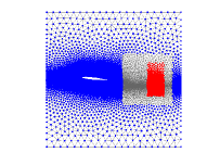
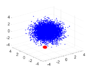
(a) Flower	(b) FEM	(c) Airfoil	(d) Set3D

Figure 3: Example 4.1. Data sets under consideration with the $\mathbf{x}$ and $\mathbf{y}$ sets marked in red and blue, respectively.

The points in the data sets are nonuniformly distributed in general, except in the case FEM where the points are more uniform. The data points in two dimensions are treated as complex numbers. The setup of the $\mathbf{x}$ and $\mathbf{y}$ sets has the size of $\mathbf{x}$ just several times larger than the target numerical rank. This is often the case in the FMM and structured solvers where the corresponding matrix blocks are short and wide off-diagonal blocks that need to be compressed in the hierarchical approximation of a global kernel matrix (see, e.g., [15, 31, 36, 38]). We consider several types of kernels as follows:

$$\kappa(x,y)=\ \frac{1}{x-y},\quad\frac{1}{(x-y)^{2}},\quad\frac{1}{|x-y|},\quad\sqrt{|x-y|+1},\quad\frac{1}{\sqrt{|x-y|^{2}+1}},$$

$$e^{-|x-y|},\quad e^{-\alpha|x-y|^{2}},\quad\log|x-y|,\quad\tan(x\cdot y+1),$$

where $\alpha$ is a parameter. Such kernels are frequently used in the FMM and in structured matrix computations like Toeplitz solutions [7] and some structured eigenvalue solvers [16, 28, 34]. For data points in three dimensions, $|x-y|$ represents the distance between $x$ and $y$.

For each data set, we apply the methods above to the kernel matrices $A$ as in (2) formed by evaluating some $\kappa(x,y)$ at $\mathbf{x}$ and $\mathbf{y}$. Most of the kernel matrices have modest numerical ranks. The schemes Nys-B, Nys-P, and Nys-R use sample sizes $S$ up to $400$ in almost all the tests. The HAN schemes use much smaller sample sizes. HAN-B and HAN-U use sample sizes $S\leq 200$ for most tests, and HAN-A uses sample sizes $S\leq 50$ for all the cases.

For some kernels evaluated at the set Flower, the relative errors $\frac{\|A-\tilde{A}\|_{2}}{\|A\|_{2}}$ in one test run are reported in Figure 4. With larger $S$, the error typically gets smaller. However, Nys-B is only able to reach modest accuracies even if $S$ is quite large. (The error curve nearly stagnate in the first row of Figure 4 with increasing $S$.) The accuracy gets better with Nys-P for some cases. Nys-R can further improve the accuracy. However, they still cannot get accuracy close to $\tau=10^{-14}$ and their error curves in the second row of Figure 4 get stuck around some small rank sizes insufficient to reach high accuracies.

In comparison, the HAN schemes usually yield much better accuracies, especially with HAN-B and HAN-A. HAN-U is often less accurate than HAN-B but is more efficient because of the fast subset update. The most remarkable result is from HAN-A, which quickly reaches accuracies around $10^{-15}$ after few sampling steps (with small overall sample sizes). The second row of Figure 4 also includes the scaled singular values $\frac{\sigma_{i}(A)}{\sigma_{1}(A)}$. We can observe that HAN-B and particularly HAN-A produce approximation errors with decay patterns very close to that of SVD.

To further confirm the accuracies, we run each scheme 100 times and report the results in Figure 5. In general, we observe that the HAN schemes are more accurate, especially HAN-B and HAN-A. The direct outcome from HAN-U is not accurate, but this is likely due to the quality of the $V$ factor in (73). In fact, most other schemes end the iteration with a low-rank approximation in (73) after one row or column pivoting step by an SRR factorization. Thus, if we apply an additional row pivoting step to $A_{:,\mathcal{J}}$ at the end of HAN-U so as to generate a new approximation $UA_{\mathcal{I},:}$ like in (73), then the resulting errors of HAN-U (called effective errors in Figure 5) are close to those of HAN-B.

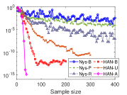
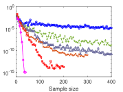
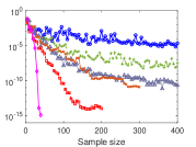
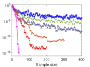
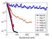
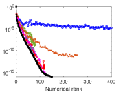
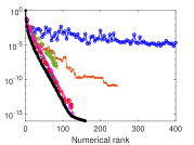
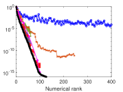
$\kappa(x,y)=\frac{1}{x-y}$	$\sqrt{|x-y|+1}$	$e^{-|x-y|}$	$\log|x-y|$

Figure 4: Example 4.1 (data set Flower): Low-rank approximation errors $\frac{\|A-\tilde{A}\|_{2}}{\|A\|_{2}}$ as the sample size $S$ increases in one test, where the second row shows the errors with respect to the resulting numerical ranks corresponding to the first row and the SVD line shows the scaled singular values.

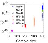
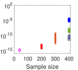
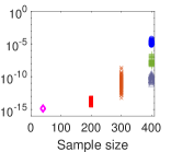
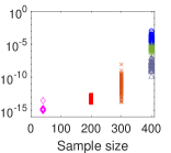
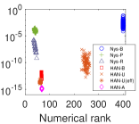
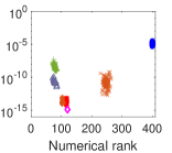
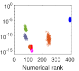
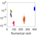
$\kappa(x,y)=\frac{1}{x-y}$	$\sqrt{|x-y|+1}$	$e^{-|x-y|}$	$\log|x-y|$

Figure 5: Example 4.1 (data set Flower): Relative errors from running the methods for $100$ times, where HAN-U(eff) is for the effective errors of HAN-U.

Similarly, for the other data sets and various different kernel functions, we have test results as given in Figures 6–11. The results can be interpreted similarly. For some cases, Nys-B, Nys-P, and even Nys-R may be quite inaccurate. One example is for $\kappa(x,y)=e^{-16|x-y|^{2}}$ in Figures 10 and 11, where even Nys-R becomes quite unreliable and demonstrates oscillatory errors for different $S$ and different tests.

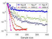
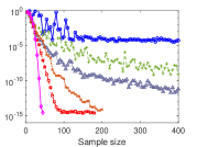
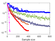
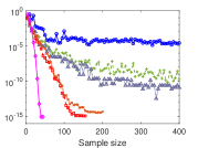
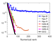
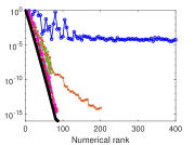
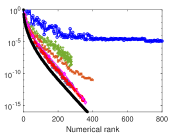
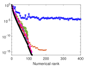
$\kappa(x,y)=\frac{1}{x-y}$	$\frac{1}{(x-y)^{2}}$	$\frac{1}{|x-y|}$	$\log|x-y|$

Figure 6: Example 4.1 (data set FEM): Low-rank approximation errors $\frac{\|A-\tilde{A}\|_{2}}{\|A\|_{2}}$ as the sample size $S$ increases in one test, where the second row shows the errors with respect to the resulting numerical ranks corresponding to the first row and the SVD line shows the scaled singular values.

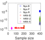
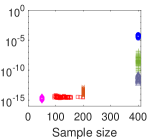
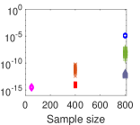
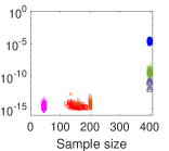
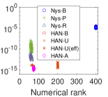
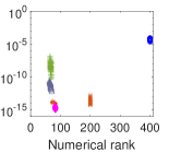
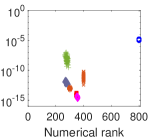
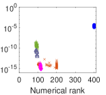
$\kappa(x,y)=\frac{1}{x-y}$	$\frac{1}{(x-y)^{2}}$	$\frac{1}{|x-y|}$	$\log|x-y|$

Figure 7: Example 4.1 (data set FEM): Relative errors from running the methods for $100$ times, where HAN-U(eff) is for the effective errors of HAN-U.

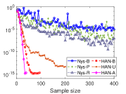
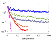
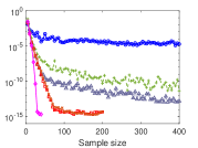
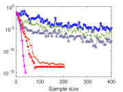
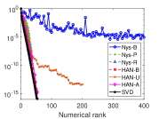
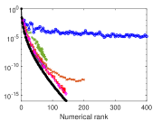
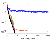
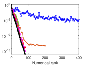
$\kappa(x,y)=\frac{1}{x-y}$	$\frac{1}{\sqrt{|x-y|^{2}+1}}$	$e^{-\frac{|x-y|^{2}}{2}}$	$\log|x-y|$

Figure 8: Example 4.1 (data set Airfoil): Low-rank approximation errors $\frac{\|A-\tilde{A}\|_{2}}{\|A\|_{2}}$ as the sample size $S$ increases in one test, where the second row shows the errors with respect to the resulting numerical ranks corresponding to the first row and the SVD line shows the scaled singular values.

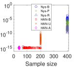
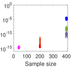
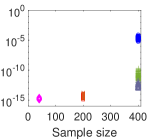
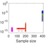
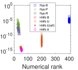
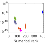
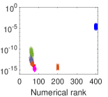
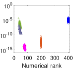
$\kappa(x,y)=\frac{1}{x-y}$	$\frac{1}{\sqrt{|x-y|^{2}+1}}$	$e^{-\frac{|x-y|^{2}}{2}}$	$\log|x-y|$

Figure 9: Example 4.1 (data set Airfoil): Relative errors from running the methods for $100$ times, where HAN-U(eff) is for the effective errors of HAN-U.

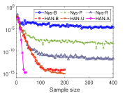
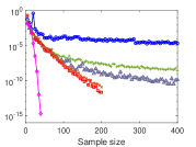
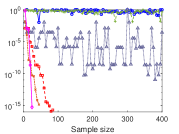
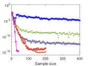
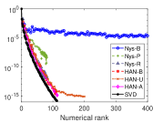
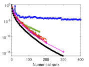
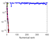
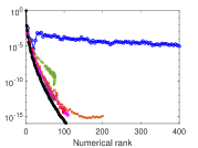
$\kappa(x,y)=\frac{1}{|x-y|}$	$\tan(x\cdot y+1)$	$e^{-16|x-y|^{2}}$	$\log|x-y|$

Figure 10: Example 4.1 (data set Set3D): Low-rank approximation errors $\frac{\|A-\tilde{A}\|_{2}}{\|A\|_{2}}$ as the sample size $S$ increases in one test, where the second row shows the errors with respect to the resulting numerical ranks corresponding to the first row and the SVD line shows the scaled singular values.

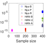
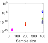
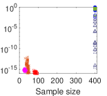
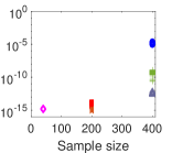
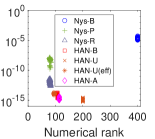
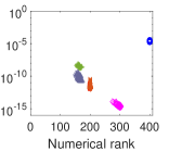
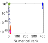
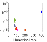
$\kappa(x,y)=\frac{1}{|x-y|}$	$\tan(x\cdot y+1)$	$e^{-16|x-y|^{2}}$	$\log|x-y|$

Figure 11: Example 4.1 (data set Set3D): Relative errors from running the methods for $100$ times, where HAN-U(eff) is for the effective errors of HAN-U.

The aggressive rank advancement also makes HAN-A very efficient. For each data set, the average timing of HAN-A and Nys-R from $100$ runs is shown in Table 1. HAN-A is generally faster than Nys-R by multiple times.

Table 1: Example 4.1. Average timing (in seconds) of HAN-A and Nys-R from $100$ runs.

Flower	$\kappa(x,y)$	$\frac{1}{x-y}$	$\sqrt{|x-y|+1}$	$e^{-|x-y|}$	$\log|x-y|$
	Nys-R	1.751	1.285	1.313	0.851
	HAN-A	0.802	0.727	0.690	0.512
FEM	$\kappa(x,y)$	$\frac{1}{x-y}$	$\frac{1}{(x-y)^{2}}$	$\frac{1}{|x-y|}$	$\log|x-y|$
	Nys-R	0.868	0.962	2.495	0.469
	HAN-A	0.191	0.193	0.607	0.108
Airfoil	$\kappa(x,y)$	$\frac{1}{x-y}$	$\frac{1}{\sqrt{|x-y|^{2}+1}}$	$e^{-\frac{|x-y|^{2}}{2}}$	$\log|x-y|$
	Nys-R	1.155	0.937	0.734	0.457
	HAN-A	0.322	0.451	0.289	0.158
Set3D	$\kappa(x,y)$	$\frac{1}{|x-y|}$	$\tan(x\cdot y+1)$	$e^{-16|x-y|^{2}}$	$\log|x-y|$
	Nys-R	0.723	1.910	0.121	0.680
	HAN-A	0.355	0.788	0.035	0.333

Example 4.2.

Next, consider a class of implicitly defined kernel matrices with varying sizes. Suppose $C$ is a circulant matrix with eigenvalues being discretized values of a function $f(t)$ at some points in an interval. Such matrices appear in some image processing problems [27], solutions of ODEs and PDEs [2, 3], and spectral methods [31]. They are usually multiplied or added to some other matrices so that the circulant structure is destroyed. However, it is shown in [31, 39] that they have small off-diagonal numerical ranks for some $f(t)$. Such rank structures are preserved under various matrix operations. The matrix $A$ we consider here is the $n\times n$ upper right corner block of $C$ (with half of the size of $C$). It is also shown in [39] that $A$ is the evaluation of an implicit kernel function over certain data points.

We consider $A$ with its size $n=512,1024,\ldots,16384$ so as to demonstrate that HAN-A can reach high accuracies with nearly linear complexity. For each $n$, we run HAN-A for $10$ times and report the outcome. As $n$ doubles, Figure 12(a) shows the numerical ranks $r$ from HAN-A, which slowly increase with $n$. This is consistent with the result in [39] where it is shown that the numerical ranks grow as a low-degree power of $\log n$. The low-rank approximation errors are given in Figure 12(b) and the average time from the $10$ runs for each $n$ is given in Figure 12(c). The runtimes roughly follow the $O(r^{2}n)$ pattern, as explained in Section 3.2.

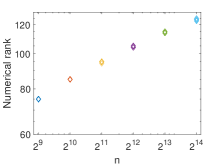
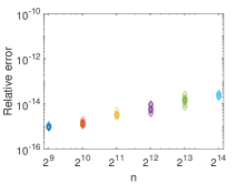
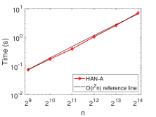
(a) Numerical rank $r$	(b) $\frac{\|A-\tilde{A}\|_{2}}{\|A\|_{2}}$	(c) Average timing

Figure 12: Example 4.2: Results from HAN-A for a type of implicitly defined kernel matrices.

Example 4.3.

Finally for completeness, we would like to show that the HAN schemes also work for high-dimensional data sets. (We remark that practical data analysis may not necessarily need very high accuracies. However, the HAN schemes can serve as a fast way to convert such data matrices into some rank structured forms that allow quick matrix operations.) We consider kernel matrices resulting from the evaluation of some kernel functions at two data sets Abalone and DryBean from the UCI Machine Learning Repository (https://archive.ics.uci.edu). The two data sets have $4177$ and $13611$ points in $8$ and $16$ dimensions, respectively. Here, each data set is standardized to have mean $0$ and variance $1$. We take the submatrix of each resulting kernel matrix formed by the first $1000$ rows so as to make it rectangular and nonsymmetric.

A set of test results is given in Figure 13. Nys-B can only reach modest accuracies around $10^{-5}$. Nys-R can indeed gets quite good accuracies. Nevertheless, HAN-A still reaches high accuracies with a small number of sampling steps. Similar results are observed with multiple runs.

(Set Abalone)		(Set DryBean)
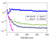
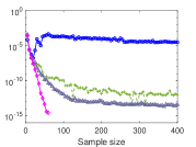
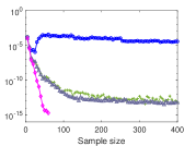
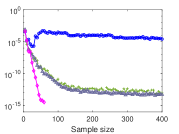
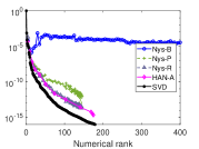
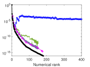
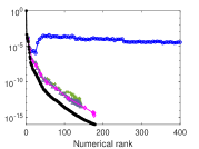
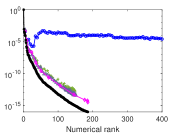
$\kappa(x,y)=\sqrt{\frac{|x-y|^{2}}{\sigma^{2}}+1}$	$e^{-\frac{|x-y|^{2}}{\sigma^{2}}}$	$\sqrt{\frac{|x-y|^{2}}{\sigma^{2}}+1}$	$e^{-\frac{|x-y|^{2}}{\sigma^{2}}}$

Figure 13: Example 4.3: Low-rank approximation errors $\frac{\|A-\tilde{A}\|_{2}}{\|A\|_{2}}$ for high-dimensional tests, where $\sigma$ in the kernel functions is set to be four times the maximum distance between the data points and the origin, and the SVD line shows the scaled singular values.

5 Conclusions

This work proposes a set of techniques that can make the Nyström method reach high accuracies in practice for kernel matrix low-rank approximations. The usual Nyström method is combined with strong rank-revealing factorizations to serve as a pivoting strategy. The low-rank basis matrices are refined through alternating direction row and column pivoting. This is incorporated into a progressive sampling scheme until a desired accuracy or numerical rank is reached. A fast subset update strategy further leads to improved efficiency and also convenient randomized accuracy control. The design of the resulting HAN schemes is based on some strong heuristics, as supported by some relevant accuracy and singular value analysis. Extensive numerical tests show that the schemes can quickly reach high accuracies, sometimes with quality close to SVDs.

The schemes are useful for low-rank approximations related to kernel matrices in many numerical computations. They can also be used in rank-structured methods to accelerate various data analysis tasks. The design of the schemes is fully algebraic and does not require particular information from the kernel or the data sets. It remains open to give statistical or deterministic analysis of the decay of the approximation error in the progressive sampling and refinement steps. We are also attempting a probabilistic study of some steps in the HAN schemes that may be viewed as a randomized rank-revealing factorization.

References

- [1] H. Avron and S. Toledo, Randomized algorithms for estimating the trace of an implicit symmetric positive semi-definite matrix, J. ACM 58 (2011), Article 8.
- [2] Z.-Z. Bai and M. K. Ng, Preconditioners for nonsymmetric block toeplitz-like-plus-diagonal linear systems, Numer. Math., 96 (2003), pp. 197–220.
- [3] Z.-Z. Bai and K.-Y. Lu, On regularized Hermitian splitting iteration methods for solving discretized almost-isotropic spatial fractional diffusion equations, 27, (2020), e2274.
- [4] M. Bebendorf, Approximation of boundary element matrices, Numer. Math., 86 (2000), pp. 565–589.
- [5] D. Cai, J. Nagy, and Y. Xi, Fast deterministic approximation of symmetric indefinite kernel matrices with high dimensional datasets, SIAM J. Matrix Anal. Appl., 43 (2022), pp. 1003–1028.
- [6] T. F. Chan, Rank revealing QR factorizations, Linear Algebra Appl., 88/89 (1987), pp. 67–82.
- [7] S. Chandrasekaran, M. Gu, X. Sun, J. Xia, and J. Zhu, A superfast algorithm for Toeplitz systems of linear equations, SIAM J. Matrix Anal. Appl., 29 (2007), pp. 1247–1266.
- [8] A. Deshpande, L. Rademacher, S. Vempala, and G. Wang, Matrix approximation and projective clustering via volume sampling, Theory Comput., 2 (2006), pp. 225–247.
- [9] P. Drineas, R. Kannan, and M. W. Mahoney, Fast Monte Carlo algorithms for matrices I: Approximating matrix multiplication, SIAM Journal on Computing 36 (2006), pp. 132–157.
- [10] P. Drineas and M. W. Mahoney, On the Nyström method for approximating a Gram matrix for improved kernel-based learning, J. Machine Learning, 6 (2005), pp. 2153–2175.
- [11] P. Drineas, M. W. Mahoney, and D. P. Woodruff, Fast approximation of matrix coherence and statistical leverage, J. Machine Learning, 13 (2012) pp. 3441–3472.
- [12] J. R. Gilbert and S.-H. Teng, MESHPART, A Matlab Mesh Partitioning and Graph Separator Toolbox, http://aton.cerfacs.fr/algor/Softs/MESHPART/.
- [13] A. Gittens and M. W. Mahoney, Revisiting the Nyström method for improved large-scale machine learning, J. Machine Learning, 16 (2016), pp. 1–65.
- [14] S. A. Goreinov and E. E. Tyrtyshnikov, The maximal-volume concept in approximation by low-rank matrices, in Contemporary Mathematics, vol 280, 2001, pp. 47–52.
- [15] L. Greengard and V. Rokhlin, A fast algorithm for particle simulations, J. Comput. Phys., 73 (1987), pp. 325–348.
- [16] M. Gu and S. C. Eisenstat, A divide-and-conquer algorithm for the symmetric tridiagonal eigenproblem, SIAM J. Matrix Anal. Appl., 16 (1995), pp. 79–92.
- [17] M. Gu and S. C. Eisenstat, Efficient algorithms for computing a strong rank-revealing QR factorization, SIAM J. Sci. Comput., 17 (1996), pp. 848–869.
- [18] W. Hackbusch, A sparse matrix arithmetic based on -matrices, Computing, 62 (1999), pp. 89–108.
- [19] N. Halko, P.G. Martinsson, and J. Tropp, Finding structure with randomness: Probabilistic algorithms for constructing approximate matrix decompositions, SIAM Review, 53 (2011), pp. 217–288.
- [20] R. A. Horn and C. R. Johnson, Topics in Matrix Analysis, Cambridge University Press, Cambridge, 1991.
- [21] I. C. F. Ipsen and T. Wentworth, Sensitivity of leverage scores and coherence for randomized matrix algorithms, Extended abstract, Workshop on Advances in Matrix Functions and Matrix Equations, Manchester, UK, 2013.
- [22] S. Kumar, M. Mohri, and A. Talwalkar, Sampling methods for the Nyström method, J. Machine Learning, 13 (2012), pp. 981–1006.
- [23] Q. Luan and V. Y. Pan, CUR LRA at sublinear cost based on volume maximization, In LNCS 11989, Book: Mathematical Aspects of Computer and Information Sciences (MACIS 2019), D. Salmanig et al (Eds.), Springer Nature Switzerland AG 2020, Chapter No: 10, pages 1–17, Springer Nature Switzerland AG 2020 Chapter.
- [24] T. Mach, L. Reichel, M. Van Barel, and R. Vandebril, Adaptive cross approximation for ill-posed problems, J. Comput. Appl. Math., 303 (2016), pp. 206–217.
- [25] P. G. Martinsson, G. Quintana-Orti, N. Heavner, and R. van de Geijn, Householder QR factorization with randomization for column pivoting (HQRRP), SIAM J. Sci. Comput., 39 (2017), pp. C96–C115.
- [26] L. Miranian and M Gu, Strong rank revealing LU factorizations, Linear Alg. Appl., 367 (2003), pp. 1–16.
- [27] J. Nagy, P. Pauca, R. Plemmons, and T. Torgersen, Space-varying restoration of optical images, J. Opt. Soc. Amer. A, 14 (1997), pp. 3162–3174.
- [28] X. Ou and J. Xia, SuperDC: Superfast divide-and-conquer eigenvalue decomposition with improved stability for rank-structured matrices, SIAM J. Sci. Comput., 44 (2022), pp. A3041–A3066.
- [29] V. Y. Pan, Q. Luan, J. Svadlenka, and L. Zhao, CUR low rank approximation of a matrix at sublinear cost, arXiv:1906.04112.
- [30] P.-O. Persson, DistMesh - A Simple Mesh Generator in MATLAB, http://persson.berkeley.edu/distmesh.
- [31] J. Shen, Y. Wang, and J. Xia, Fast structured direct spectral methods for differential equations with variable coefficients, I. The one-dimensional case, SIAM J. Sci. Comput., 38 (2016), pp. A28–A54.
- [32] A. Talwalkar and A. Rostamizadeh, Matrix coherence and the Nyström method, UAI’10: Proceedings of the Twenty-Sixth Conference on Uncertainty in Artificial Intelligence, (2010), pp. 572–579.
- [33] J. A. Tropp, A. Yurtsever, M. Udell, and V. Cevher, Practical sketching algorithms for low-rank matrix approximation, SIAM J. Matrix Anal. Appl., 38 (2017), pp. 1454–1485.
- [34] J. Vogel, J. Xia, S. Cauley, and V. Balakrishnan, Superfast divide-and-conquer method and perturbation analysis for structured eigenvalue solutions, SIAM J. Sci. Comput., 38 (2016), pp. A1358–A1382.
- [35] C. Williams and M. Seeger, Using the Nyström method to speed up kernel machines, Advances in Neural Information Processing Systems 13, (2001), pp. 682–688.
- [36] J. Xia, Randomized sparse direct solvers, SIAM J. Matrix Anal. Appl., 34 (2013), pp. 197–227.
- [37] J. Xia, Multi-layer hierarchical structures, CSIAM Trans. Appl. Math., 2 (2021), pp. 263–296.
- [38] J. Xia, S. Chandrasekaran, M. Gu, and X. S. Li, Fast algorithms for hierarchically semiseparable matrices, Numer. Linear Algebra Appl., 17 (2010), pp. 953–976.
- [39] J. Xia and M. Lepilov, Why are many circulant matrices rank structured? Preprint.
- [40] J. Xiao, M. Gu, and J. Langou, Fast parallel randomized QR with column pivoting algorithms for reliable low-rank matrix approximations, 24th IEEE International Conference on High Performance Computing, Data, and Analytics (HIPC), Jaipur, India, 2017.
- [41] X. Ye, J. Xia, and L. Ying, Analytical low-rank compression via proxy point selection, SIAM J. Matrix Anal. Appl., 41 (2020), pp. 1059–1085.
- [42] K. Zhang, I. W. Tsang, and J. T. Kwok, Improved Nyström low-rank approximation and error analysis, Proceedings of the 25th international conference on Machine learning, (2008), pp. 1232–1239.