The Dependence of Iron-rich Metal-poor Star Occurrence on Galactic Environment Supports an Origin in Thermonuclear Supernova Nucleosynthesis

Abstract

It has been suggested that a class of chemically peculiar metal-poor stars called iron-rich metal-poor (IRMP) stars formed from molecular cores with metal contents dominated by thermonuclear supernova nucleosynthesis. If this interpretation is accurate, then IRMP stars should be more common in environments where thermonuclear supernovae were important contributors to chemical evolution. Conversely, IRMP stars should be less common in environments where thermonuclear supernovae were not important contributors to chemical evolution. At constant $[\text{Fe/H}]\lesssim-1$, the Milky Way’s satellite classical dwarf spheroidal (dSph) galaxies and the Magellanic Clouds have lower $[\text{$\alpha$/Fe}]$ than the Milky Way field and globular cluster populations. This difference is thought to demonstrate the importance of thermonuclear supernova nucleosynthesis for the chemical evolution of the Milky Way’s satellite classical dSph galaxies and the Magellanic Clouds. We use data from the Sloan Digital Sky Survey (SDSS) Apache Point Observatory Galactic Evolution Experiment (APOGEE) and Gaia to infer the occurrence of IRMP stars in the Milky Way’s satellite classical dSph galaxies $\eta_{\text{dSph}}$ and the Magellanic Clouds $\eta_{\text{Mag}}$ as well as in the Milky Way field $\eta_{\text{MWF}}$ and globular cluster populations $\eta_{\text{MWGC}}$. In order of decreasing occurrence, we find $\eta_{\text{dSph}}=0.07_{-0.02}^{+0.02}$, $\eta_{\text{Mag}}=0.037_{-0.006}^{+0.007}$, $\eta_{\text{MWF}}=0.0013_{-0.0005}^{+0.0006}$, and a 1-$\sigma$ upper limit $\eta_{\text{MWGC}}<0.00057$. These occurrences support the inference that IRMP stars formed in environments dominated by thermonuclear supernova nucleosynthesis and that the time lag between the formation of the first and second stellar generations in globular clusters was longer than the thermonuclear supernova delay time.

Astronomical Journal

1 Introduction

Thermonuclear supernovae are prolific producers of iron-peak elements with a theoretically predicted average stable yield of more than $0.6~{}M_{\odot}$ of iron-peak elements but much less $\alpha$ and light odd-$Z$ elements. This is in sharp contrast to core-collapse supernovae that produce $\alpha$ and light odd-$Z$ elements in roughly the solar ratios but with relatively little iron-peak production (e.g., Sukhbold et al., 2016).

Based on a compilation of theoretical stable nucleosynthetic yields predicted by a variety of thermonuclear supernova progenitor channels (i.e., single degenerate and double degenerate) and explosion mechanisms (e.g., pure detonations, pure deflagrations, delayed detonations, double detonations, etc.), Reggiani et al. (2023) proposed the existence of a new class of chemically peculiar metal-poor stars with $[\text{Fe/H}]\lesssim-1$ and $[\text{O,F,Ne,Na,Mg,Al,Cl,K,Co,Cu,Zn/Fe}]<0$ formed from molecular cores with metal contents dominated by thermonuclear supernova nucleosynthesis. They called stars with these properties iron-rich metal-poor (IRMP) stars, as this part of elemental abundance space is consistent with thermonuclear supernova nucleosynthesis but rarely observed in metal-poor stars. They argued that if their interpretation is correct, then IRMP stars should be more common in environments where thermonuclear supernovae were relatively more important contributors to chemical evolution relative to core-collapse supernovae (e.g., environments with long star formation durations). On the other hand, they argued that in environments where thermonuclear supernovae were not important contributors to chemical evolution relative to core-collapse supernovae (e.g., environments with short star formation durations) IRMP stars should be less common.

One way to test this prediction would be to compare the relative occurrence of IRMP stars in the Milky Way’s field population, its globular clusters, its satellite classical dwarf spheroidal (dSph) galaxies, and the Magellanic Clouds. At constant spectroscopically inferred metallicities $[\text{Fe/H}]\lesssim-1$, both the Milky Way’s classical dSph satellites (Shetrone et al., 2001, 2003; Tolstoy et al., 2003; Kirby et al., 2009, 2010, 2011a, 2011b) and the Magellanic Clouds (Pompéia et al., 2008; Van der Swaelmen et al., 2013; Nidever et al., 2020) have lower spectroscopically inferred ratios of the $\alpha$ elements oxygen, magnesium, silicon, and calcium to iron $[\text{$\alpha$/Fe}]$ than the Milky Way (e.g., Wallerstein, 1962; Luck & Bond, 1981, 1985; Peterson, 1981; Gratton, 1983; Magain, 1985, 1989; Gratton & Ortolani, 1986; Gratton & Sneden, 1988; Ryan et al., 1991; McWilliam et al., 1995a, b) and its globular clusters (e.g., Cohen, 1978, 1979, 1980, 1981; Pilachowski et al., 1983). These offsets in $[\text{$\alpha$/Fe}]$ between the Milky Way field & globular cluster populations and its satellite classical dSph galaxies & the Magellanic Clouds are usually understood to indicate the longer durations of low-metallicity star formation and therefore the relatively more important contributions of thermonuclear supernovae to the chemical evolution of the latter two environments at low metallicities (e.g., Lanfranchi & Matteucci, 2003, 2004, 2007; Lanfranchi et al., 2006, 2008; Marcolini et al., 2006; Kirby et al., 2011a; Bekki & Tsujimoto, 2012; Nidever et al., 2020; Reggiani et al., 2021). If the Reggiani et al. (2023) interpretation of IRMP stars is valid, then IRMP stars should be less common in the Milky Way field & globular cluster populations than in its satellite classical dSph galaxies & the Magellanic Clouds.

The nitrogen, sodium, and aluminum abundances of individual stars in globular clusters have been found to be anticorrelated with the carbon, oxygen, and magnesium abundances in the same stars. These abundance anticorrelations have been interpreted as evidence for multiple generations of star formation in globular clusters (e.g., Sneden et al., 1992; Gratton et al., 2001, 2004; Carretta et al., 2009; Bastian & Lardo, 2018). The Reggiani et al. (2023) interpretation of IRMP stars also suggests the possibility that the occurrence of IRMP stars in globular clusters can be used to constrain the time lag between the formation of a globular cluster’s first and second stellar generations. For Type Ia supernovae delay times $\tau_{\text{Ia}}\lesssim 100$ Myr, the Type Ia supernova rate $\Phi_{\text{Ia}}$ has the value $\Phi_{\text{Ia}}\sim 10^{-12}$ yr^-1 $M_{\odot}^{-1}$ (e.g., Totani et al., 2008; Maoz et al., 2011, 2012, 2014; Graur et al., 2014). Assuming that rate and a typical first generation initial globular cluster mass $M_{\text{MWGC}}\sim 10^{6}~{}M_{\odot}$ (e.g., Conroy, 2012), order 10 Type Ia supernovae should occur in a newly formed globular cluster every 10 Myr after the Type Ia delay time has elapsed. While the occurrence of the short-period binaries necessary to produce most of the theoretically predicted thermonuclear supernova progenitor systems is a factor of about three lower in globular clusters’ first generations than in the field (Carney et al., 2003; Lucatello et al., 2015), after the Type Ia supernovae delay time has elapsed a few thermonuclear explosions should occur every 10 Myr during the formation of a globular cluster. The Reggiani et al. (2023) interpretation of IRMP stars therefore implies that if the time lag between the formation of first and second generation stars in globular clusters was shorter than the typical thermonuclear supernova delay time, then the occurrence of IRMP stars in globular clusters should be significantly lower than in the Milky Way field. If the the time lag between the formation of first and second generation stars in globular clusters is longer than the typical thermonuclear supernova delay time, then the occurrence of IRMP stars in globular clusters and the Milky Way field should be comparable.

We argue that if the Reggiani et al. (2023) interpretation of the origin of IRMP stars is accurate, then the occurrence of IRMP stars in the Milky Way field population $\eta_{\text{MWF}}$, the Magellanic Clouds $\eta_{\text{Mag}}$, and the Milky Way’s satellite classical dSph galaxies $\eta_{\text{dSph}}$ should be ordered $\eta_{\text{MWF}}<\eta_{\text{Mag}}\sim\eta_{\text{dSph}}$. If the time lag between the formation of the first and second generations in globular clusters was shorter than the thermonuclear supernova delay time, then the occurrence of IRMP stars in the Milky Way globular cluster population $\eta_{\text{MWGC}}$ should be $\eta_{\text{MWGC}}\lesssim\eta_{\text{MWF}}<\eta_{\text{Mag}}\sim\eta_{\text{dSph}}$. If the time lag between the formation of the first and second generations in globular clusters was longer than the thermonuclear supernova delay time, then $\eta_{\text{MWGC}}\sim\eta_{\text{MWF}}<\eta_{\text{Mag}}\sim\eta_{\text{dSph}}$. In this article, we calculate the occurrence of IRMP stars in the Milky Way’s satellite classical dSph galaxies, the Magellanic Clouds, the Milky Way field population, and in Milky Way globular clusters. We describe in Section 2 the assembly of our analysis samples and quantify in Section 3 the occurrence of IRMP stars in each environment. We review the implications of those occurrences in Section 4 and conclude by summarizing our findings in Section 5.

2 Data

To calculate the occurrence of IRMP stars in the Milky Way’s satellite classical dSph galaxies, the Magellanic Clouds, the Milky Way field population, and in Milky Way globular clusters we use data derived from spectra that were gathered during the third and fourth phases of the Sloan Digital Sky Survey (SDSS; Eisenstein et al., 2011; Blanton et al., 2017) as part of its Apache Point Observatory Galactic Evolution Experiment (APOGEE; Majewski et al., 2017). These spectra were collected with the APOGEE spectrographs (Zasowski et al., 2013, 2017; Wilson et al., 2019; Beaton et al., 2021; Santana et al., 2021) on the New Mexico State University 1-m Telescope (Holtzman et al., 2010), the Sloan Foundation 2.5-m Telescope (Gunn et al., 2006), and the 2.5-m Irénée du Pont Telescope (Bowen & Vaughan, 1973). As part of SDSS Data Release (DR) 17 (Abdurro’uf et al., 2022), these spectra were reduced and analyzed with the APOGEE Stellar Parameter and Chemical Abundance Pipeline (ASPCAP; Allende Prieto et al., 2006; Holtzman et al., 2015; Nidever et al., 2015; García Pérez et al., 2016) using an $H$-band line list, MARCS model atmospheres, and model-fitting tools optimized for the APOGEE effort (Alvarez & Plez, 1998; Gustafsson et al., 2008; Hubeny & Lanz, 2011; Plez, 2012; Smith et al., 2013, 2021; Cunha et al., 2015; Shetrone et al., 2015; Jönsson et al., 2020).

We use the CasJobs portal and the query described in the Appendix to generate our initial sample of photospheric stellar parameters and elemental abundances for giant stars with $\log{g}<3.8$. As described in the Appendix, we use a carefully curated set of data quality flags to ensure the accuracy and precision of those photospheric stellar parameters and elemental abundances. We set to null any elemental abundance/elemental abundance uncertainty pair that does not pass the data quality checks described in the Appendix. Corrections for departures from local thermodynamic equilibrium are usually small for $H$-band elemental abundance inferences (e.g., Osorio et al., 2020), and we choose not to apply them in our analysis.

Following Reggiani et al. (2023), we define an iron-rich metal-poor star as a star with $[\text{Fe/H}]<-1$ and $[\text{O,Na,Mg,Al,K,Co/Fe}]<0$. Those elemental abundance ratios form the intersection of the IRMP criteria defined in Reggiani et al. (2023) and the list of elemental abundances reliably inferred for giant stars as part of APOGEE DR17. For the purposes of the occurrence calculation described in the next section, an IRMP star with $[\text{Fe/H}]<-1$ must have at least one non-null abundance ratio $[\text{O/Fe}]$, $[\text{Na/Fe}]$, $[\text{Mg/Fe}]$, $[\text{Al/Fe}]$, $[\text{K/Fe}]$, or $[\text{Co/Fe}]$ and all abundance ratios $[\text{O,Na,Mg,Al,K,Co/Fe}]$ either sub-solar or null.

To accurately label stars with their correct galactic environments, we first join the APOGEE data described above with data from Gaia DR2 (Gaia Collaboration et al., 2016, 2018; Arenou et al., 2018; Evans et al., 2018; Lindegren et al., 2018; Luri et al., 2018; Riello et al., 2018) and DR3 (Gaia Collaboration et al., 2016, 2021; Fabricius et al., 2021; Lindegren et al., 2021a, b; Riello et al., 2021; Rowell et al., 2021; Torra et al., 2021). We use the apogee_id string to identify the corresponding Gaia DR2 and DR3 source_id long integers by joining with the gaiadr2.tmass_best_neighbour and gaiadr3.tmass_psc_xsc_best_neighbour tables available in the Gaia archive (Salgado et al., 2017; Marrese et al., 2019). Occasionally multiple Gaia DR2 and DR3 source_id long integers are matched to the same object in the 2MASS Point Source Catalog (Skrutskie et al., 2006). In those cases, we associate a 2MASS object with the closest Gaia DR2 and DR3 object that has (1) an absolute 2MASS $K_{\text{s}}$-band magnitude $M_{K}<2.31$ assuming Gaia DR2- or DR3-prior informed geometric distances (Bailer-Jones et al., 2018, 2021) and (2) Gaia–2MASS colors $0.5<G-J<2.3$, $0.6<G-H<3.3$, and $0.6<G-K_{\text{s}}<3.4$ predicted by the MESA Isochrones & Stellar Tracks (MIST) grid for metal-poor giants in the range $-2.5<[\text{Fe/H}]<-1.0$ (Paxton et al., 2011, 2013, 2015, 2018; Dotter, 2016; Choi et al., 2016).

We then use the Gaia DR2 source_id to identify Milky Way satellite classical dSph galaxies or Magellanic Clouds members using the Gaia DR2-based membership lists published in Gaia Collaboration et al. (2018). We identify globular cluster members using the Gaia DR3 source_id and the Vasiliev & Baumgardt (2021) lists of stars with globular cluster membership probability greater than 0.5, and this procedure results in a sample with at least one star from 41 globular clusters over the metallicity range $-2.3\lesssim[\text{Fe/H}]\lesssim-1.0$.

Most stars observed as part SDSS-III/APOGEE and SDSS-IV/APOGEE-2 were selected for observation by a procedure that sought to minimize age and metallicity biases (e.g., Zasowski et al., 2013, 2017), and we use the targeting flag extratarg = 0 in the table apogeeStar to select those stars for our Milky Way field sample. To ensure the cleanest Milky Way field sample possible, we then remove from this sample any stars that are identified as dSph, Magellanic Cloud, or globular cluster members in Gaia Collaboration et al. (2018) or Vasiliev & Baumgardt (2021). Because the vast majority of stars with $[\text{Fe/H}]\lesssim-1$ observed as part of SDSS-III/APOGEE and SDSS-IV/APOGEE-2 are on halo-like orbits (e.g., Hayes et al., 2018), our Milky Way field sample can be thought of as a Milky Way halo sample. We list in Table 1 our entire analysis sample including IRMP status and galactic environment. We report in Table 2 the number of stars classified as IRMP stars in each environment $N_{\ast,\text{IRMP}}$ along with the number of stars in our analysis sample in each environment $N_{\ast,\text{tot}}$.

Table 1: Analysis Sample

APOGEE ID	Gaia DR3 source_id	Gaia DR2 source_id	IRMP	Environment
2M17165079$-$2422565	4111066558908989184	4111066558908989184	False	Milky Way
2M17150296$-$2423503	4114045307692005632	4114045307692005632	False	Milky Way
2M19154424$-$0604209	4211181280154376320	4211181280154376320	False	Milky Way
2M19033822$+$1745138	4514220364269464832	4514220364269464832	False	Milky Way
2M16574858$-$2156135	4126283868512500864	4126283868512500864	False	Milky Way
2M18501947$+$2948368	2041393317228382848	2041393317228382848	False	Milky Way
2M18132084$+$0112054	4275831399934633984	4275831399934633984	False	Milky Way
2M17571005$-$3020262	4056215664653907456	4056215664653907456	False	Milky Way
2M17415271$-$2715374	4060889448072712832	4060889448072712832	False	Milky Way
2M19084424$-$0618527	4205916204326948736	4205916204326948736	False	Milky Way

Note. — This table is published in its entirety in the machine-readable format. A portion is shown here for guidance regarding its form and content.

Table 2: Occurrence of IRMP Stars as a Function of Environment

Galactic Environment	$N_{\ast,\text{IRMP}}$	$N_{\ast,\text{tot}}$	Occurrence
Milky Way	5	4247	$0.0013_{-0.0005}^{+0.0006}$
Globular Cluster Sum	0	1998	$<0.00057$
LMC	4	203	$0.023_{-0.009}^{+0.012}$
SMC	24	572	$0.043_{-0.008}^{+0.009}$
Magellanic Clouds Sum	28	775	$0.037_{-0.006}^{+0.007}$
Sagittarius	0	27	$<0.04$
Ursa Minor	0	8	$<0.12$
Sextans	1	6	$0.2_{-0.1}^{+0.2}$
Sculptor	8	70	$0.12_{-0.03}^{+0.04}$
Draco	0	9	$<0.11$
Carina	1	31	$0.05_{-0.03}^{+0.05}$
dSph Galaxies Sum	10	151	$0.07_{-0.02}^{+0.02}$

The typical elemental abundance inference uncertainties in our analysis sample are (0.04, 0.23, 0.03, 0.04, 0.08, 0.16) dex for ($[\text{O/Fe}]$, $[\text{Na/Fe}]$, $[\text{Mg/Fe}]$, $[\text{Al/Fe}]$, $[\text{K/Fe}]$, $[\text{Co/Fe}]$). In any case, elemental abundance inference uncertainties are irrelevant for the occurrence analyses presented in Section 3 if (1) the uncertainty distributions for each elemental abundance inference for each individual star are symmetric and (2) the uncertainty distributions have statistically indistinguishable widths across all of the galactic environments we explored. The individual elemental abundance inference uncertainties presented in the SDSS DR17 version of the table aspcapStar are reported as symmetric. Additionally, we confirmed that the individual elemental abundance uncertainty distributions for oxygen, sodium, magnesium, aluminum, potassium, and cobalt have statistically indistinguishable widths across all of the galactic environments we explored. Both of the conditions listed above are therefore met in our analysis sample. Likewise, we argue that our procedure to handle data quality issues will not bias the occurrence analyses we present in Section 3. The reason is that null values impact less than about 0.2% of the magnesium abundance inferences in our sample. Because we require all non-null elemental inferences to meet our IRMP criteria, we are able to exclude essentially all non-IRMP stars from our IRMP sample using magnesium alone almost regardless of data quality issues.

The recent discovery of a very metal-poor star with elemental abundances best explained by the nucleosynthesis expected in a pair-instability supernova has focused attention on that explanation for stars with significantly subsolar $[\text{Na/Fe}]$ and $[\text{$\alpha$/Fe}]$ abundance ratios (Xing et al., 2023). While the stars in our analysis sample have subsolar $[\text{Na/Fe}]$ and the $\alpha$-element abundance ratios $[\text{O/Fe}]$ and $[\text{Mg/Fe}]$, none of the stars in our sample have the strong odd–even abundance ratios predicted to be produced by pair-instability supernovae (e.g., Heger & Woosley, 2002). We are therefore confident that the IRMP stars we identify are related to thermonuclear supernovae.

3 Analysis

We model the number of IRMP stars $N_{\ast,\text{IRMP}}$ in a sample of $N_{\ast,\text{tot}}$ candidates using a binomial distribution. Following Schlaufman (2014) we exploit the fact that a Beta$(\alpha$,$\beta$) distribution is a conjugate prior to the binomial distribution and will result in a Beta distribution posterior for the occurrence of IRMP stars in a sample. Bayes’s Theorem guarantees

$$f(\theta|\mathbf{y}) = \frac{f(\mathbf{y}|\theta)f(\theta)}{\int f(\mathbf{y}|\theta)f(\theta)d\theta},$$ (1)

where $f(\theta|\mathbf{y})$ is the posterior distribution of the model parameter $\theta$, $f(\mathbf{y}|\theta)$ is the likelihood of the data $\mathbf{y}$ given $\theta$, and $f(\theta)$ is the prior for $\theta$. In this case, the likelihood is the binomial likelihood that describes the probability of a number of successes $y$ in $n$ Bernoulli trials each with probability $\theta$ of success

$$f(y|\theta)=\left(\begin{array}[]{cc}n\\ y\end{array}\right)\theta^{y}\left(1-\theta\right)^{n-y}.$$ (4)

As shown by Schlaufman (2014), in this situation using a Beta($\alpha$,$\beta$) prior on $\theta$ with hyperparameters $\alpha$ and $\beta$ results in a Beta posterior for $\theta$ of the form Beta($\alpha+N_{\ast,\text{IRMP}},\beta+N_{\ast,\text{tot}}-N_{\ast,\text{IRMP}}$).

The hyperparameters $\alpha$ and $\beta$ of the prior can be thought of as encoding a certain amount of prior information in the form of pseudo-observations. Specifically, $\alpha-1$ is the number of success and $\beta-1$ is the number of failures imagined to have already been observed and therefore included as prior information on $\theta$. Taking any $\alpha=\beta=i$ where $i\geq 1$ could be thought of as an uninformative prior in the sense that the probability of success and failure in the prior distribution are equally likely. However, if $i$ is large then there is imagined to be a lot of prior information and the posterior distribution will mostly reflect the prior when $n\leq i$. On the other hand, if $n\gg i$, then the posterior will be dominated by the data. For that reason, we take $\alpha=\beta=1$.

We provide the posterior median occurrence of IRMP stars in each galactic environment in Table 2. We define the lower uncertainty as the difference between the posterior median and its 16th percentile. Likewise, we define the upper uncertainty as the difference between the posterior’s 84th percentile and its median. For an environment with no IRMP stars, we report 1-$\sigma$ upper limits as the 68th percentile of the posterior distribution. We find that $\eta_{\text{dSph}}=0.07_{-0.02}^{+0.02}$, $\eta_{\text{Mag}}=0.037_{-0.006}^{+0.007}$, $\eta_{\text{MWF}}=0.0013_{-0.0005}^{+0.0006}$, and a 1-$\sigma$ upper limit $\eta_{\text{MWGC}}<0.00057$. In words, IRMP stars are much more common in the Milky Way’s classical dSph satellites and the Magellanic Clouds than in the Milky Way field or globular cluster populations. IRMP stars are less common in globular clusters than in any other galactic environment. We find that the overlap probability between the IRMP occurrences we observed in the Milky Way’s classical dSph satellites and the Magellanic Clouds is about one in 91, equivalent to about 2.3 $\sigma$. We find that the overlap probabilities between the IRMP occurrences we observe in the Milky Way’s classical dSph satellites & the Magellanic Clouds and the occurrence of IRMP stars we observe in the Milky Way field population are about one in $2.8\times 10^{15}$ and one in $6.2\times 10^{19}$, equivalent to about 8.1 and 9.2 $\sigma$. The overlap probability between the IRMP occurrences we observe in the Milky Way field and globular cluster populations is about one in 23, equivalent to about 1.7 $\sigma$. We summarize these occurrence posterior overlap probabilities in Table 3.

Table 3: Occurrence Posterior Overlap Probabilities

Population	Population	$P(\text{Posterior Overlap})$
dSph galaxies	Magellanic Clouds	1.095 ×10^-2
dSph galaxies	Milky Way field	3.596 ×10^-16
Magellanic Clouds	Milky Way field	1.620 ×10^-20
Milky Way field	Milky Way globular clusters	4.300 ×10^-2

The results presented in Table 2 are averaged over metallicity. To investigate IRMP occurrence as a function of metallicity, for each class of galactic environment we divide into ten equal intervals the metallicity range spanned by our analysis sample for that environment. We then apply the same occurrence formalism in each individual metallicity interval and plot occurrence as a function of metallicity for each environment in Figure 1. We find no significant dependence of the occurrence of IRMP stars on metallicity in our analysis sample.

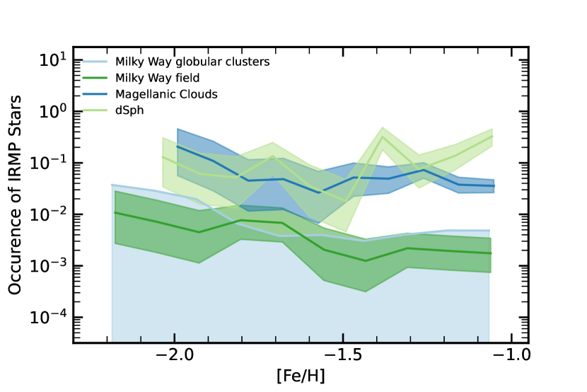
Figure 1: Occurrence of iron-rich metal-poor stars as a function of metallicity in different environments. For the Milky Way field, dSph, and Magellanic Cloud samples we plot the posterior medians of occurrence as solid lines and the ranges defined by the 16th and 84th percentiles of the occurrence posteriors as transparent polygons. For the globular cluster sample for which we infer an upper limit on IRMP occurrence, we plot the 68th percentile of the posterior as a solid line and the range defined by the 0th and 68th percentiles of the occurrence posterior as a transparent polygon. There is no obvious dependence of IRMP occurrence on metallicity in the Milky Way’s field population, its globular clusters, its classical dSph galaxies, or the Magellanic Clouds.

4 Discussion

We find that the occurrences of IRMP stars in the Milky Way’s satellite classical dSph galaxies, the Magellanic Clouds, the Milky Way field population, and the Milky Way’s globular cluster populations have the values $\eta_{\text{dSph}}=0.07_{-0.02}^{+0.02}$, $\eta_{\text{Mag}}=0.037_{-0.006}^{+0.007}$, $\eta_{\text{MWF}}=0.0013_{-0.0005}^{+0.0006}$, and $\eta_{\text{MWGC}}<0.00057$. The probability that the IRMP occurrences in the Milky Way’s satellite classical dSph galaxies and the Magellanic Clouds overlap is about one in 91, equivalent to about 2.3 $\sigma$. The probabilities that the IRMP occurrence posterior for the Milky Way field overlaps with the IRMP occurrence posteriors for Milky Way’s satellite classical dSph galaxies and the Magellanic Clouds are about one in $2.8\times 10^{15}$ and one in $6.2\times 10^{19}$, equivalent to about 8.1 and 9.2 $\sigma$. The probability that the IRMP occurrences in the Milky Way field and globular cluster populations overlap is about one in 23, equivalent to about 1.7 $\sigma$. While the absolute values of IRMP star occurrences may be difficult to interpret, as we argued in the introduction their ordering $\eta_{\text{MWGC}}\sim\eta_{\text{MWF}}<\eta_{\text{Mag}}\sim\eta_{\text{dSph}}$ has two important implications.

The increased occurrence of IRMP stars in environments like the Milky Way’s satellite classical dSph galaxies and the Magellanic Clouds where thermonuclear supernovae were important contributors to chemical evolution supports the Reggiani et al. (2023) scenario for IRMP star formation in molecular cores with metal contents dominated by the thermonuclear supernova nucleosynthesis. The confirmation of this Reggiani et al. (2023) prediction reinforces the idea that the elemental abundances of individual IRMP stars can be used to investigate the progenitor systems and explosion mechanisms responsible for the thermonuclear supernovae that produced much of their metal contents.

The statistically indistinguishable occurrences of IRMP stars in the Milky Way’s field and globular cluster populations suggests that the time lags between the formation of globular clusters’ first and second stellar generations were longer than the thermonuclear supernova delay time. This is broadly consistent with the idea from the asymptotic giant branch (AGB) scenario for globular cluster multiple populations that the explosions of thermonuclear supernovae associated with a globular cluster’s first stellar generation quench the star formation event that produced its second stellar generation (e.g., D’Ercole et al., 2008; Calura et al., 2019; Lacchin et al., 2021). Given the suspected importance of thermonuclear supernovae for quenching second generation star formation in globular clusters, it remains to be explained why globular cluster second generation stars that bear the imprint of thermonuclear supernova nucleosynthesis are so rare as to not appear in a sample of nearly 2000 globular cluster members. Our result is also consistent with scenarios for globular cluster multiple populations invoking a thermonuclear supernova at the start of a cluster’s evolution (e.g., Marcolini et al., 2009; Sánchez-Blázquez et al., 2012).

Contributions from both core-collapse and thermonuclear supernovae as well as $s$- and $r$-process nucleosynthesis are required to explain the solar abundance pattern. While the progenitors of core-collapse supernovae are known to be massive stars and the $s$-process takes place in AGB stars, the progenitors of thermonuclear supernovae and the astrophysical site of the $r$-process are more uncertain. Observational constraints on either the progenitors of thermonuclear supernovae or the astrophysical site of the $r$-process are therefore valuable. The kilonova GW170817 confirmed that neutron stars mergers are at least partially responsible for $r$-process nucleosynthesis (e.g., Abbott et al., 2017; Arcavi et al., 2017). The relative occurrences of IRMP and $r$-process enhanced stars in the same populations can be used to compare the relative probabilities of the circumstances that lead to the formation of IRMP and $r$-process enhanced stars.

We find that the occurrences of IRMP stars are an order of magnitude lower than the occurrence of $r$-process enhanced stars in both the Milky Way field and Magellanic Clouds. In the Milky Way field, we find that $\eta_{\text{IRMP,MWF}}=0.0013_{-0.0005}^{+0.0006}$ while Barklem et al. (2005) found $\eta_{\text{rII,MWF}}\approx 0.03$ according to the definition of highly $r$-process enhanced (i.e., r-II stars) from Beers & Christlieb (2005). In the Magellanic Clouds, we find that $\eta_{\text{IRMP,Mag}}=0.037_{-0.006}^{+0.007}$ while Reggiani et al. (2021) found $\eta_{\text{rII,Mag}}=0.38^{+0.14}_{-0.13}$. We conclude that the circumstances that lead to the formation of IRMP stars occur an order of magnitude less frequently than the circumstances that lead to the formation of $r$-process enhanced stars.

5 Conclusion

We conclude that iron-rich metal-poor stars with $[\text{Fe/H}]\lesssim-1$ and $[\text{O,Na,Mg,Al,K,Co/Fe}]<0$ are more common in the Milky Way’s satellite classical dSph galaxies and the Magellanic Clouds than in the Milky Way field or globular cluster populations. Because thermonuclear supernovae are thought to have been more important contributors to the chemical evolution of the Milky Way’s satellite classical dSph galaxies and the Magellanic Clouds than to the Milky Way field and globular cluster populations in the range $[\text{Fe/H}]\lesssim-1$, our inferences confirm the interpretation of iron-rich metal-poor stars put forward in Reggiani et al. (2023) proposing that iron-rich metal-poor stars formed from molecular cores with metal contents dominated by thermonuclear supernova nucleosynthesis. Iron-rich metal-poor stars can therefore be used to constrain the progenitor systems and explosion mechanisms of the thermonuclear supernovae responsible for their elemental abundances. We further find that the occurrences of iron-rich metal-poor stars in the Milky Way’s field and globular cluster populations are statistically indistinguishable. This observation implies that the time lag between the formation of a globular cluster’s first and second stellar generations was longer than the thermonuclear supernova delay time. It is also consistent with explanations for globular cluster multiple populations that require early enrichment by thermonuclear supernovae.

References

- Abbott et al. (2017) Abbott, B. P., Abbott, R., Abbott, T. D., et al. 2017, Phys. Rev. Lett., 119, 161101, doi: 10.1103/PhysRevLett.119.161101
- Abdurro’uf et al. (2022) Abdurro’uf, Accetta, K., Aerts, C., et al. 2022, ApJS, 259, 35, doi: 10.3847/1538-4365/ac4414
- Allende Prieto et al. (2006) Allende Prieto, C., Beers, T. C., Wilhelm, R., et al. 2006, ApJ, 636, 804, doi: 10.1086/498131
- Alvarez & Plez (1998) Alvarez, R., & Plez, B. 1998, A&A, 330, 1109. https://arxiv.org/abs/astro-ph/9710157
- Arcavi et al. (2017) Arcavi, I., Hosseinzadeh, G., Howell, D. A., et al. 2017, Nature, 551, 64, doi: 10.1038/nature24291
- Arenou et al. (2018) Arenou, F., Luri, X., Babusiaux, C., et al. 2018, A&A, 616, A17, doi: 10.1051/0004-6361/201833234
- Astropy Collaboration et al. (2013) Astropy Collaboration, Robitaille, T. P., Tollerud, E. J., et al. 2013, A&A, 558, A33, doi: 10.1051/0004-6361/201322068
- Astropy Collaboration et al. (2018) Astropy Collaboration, Price-Whelan, A. M., Sipőcz, B. M., et al. 2018, AJ, 156, 123, doi: 10.3847/1538-3881/aabc4f
- Bailer-Jones et al. (2021) Bailer-Jones, C. A. L., Rybizki, J., Fouesneau, M., Demleitner, M., & Andrae, R. 2021, AJ, 161, 147, doi: 10.3847/1538-3881/abd806
- Bailer-Jones et al. (2018) Bailer-Jones, C. A. L., Rybizki, J., Fouesneau, M., Mantelet, G., & Andrae, R. 2018, AJ, 156, 58, doi: 10.3847/1538-3881/aacb21
- Barklem et al. (2005) Barklem, P. S., Christlieb, N., Beers, T. C., et al. 2005, A&A, 439, 129, doi: 10.1051/0004-6361:20052967
- Bastian & Lardo (2018) Bastian, N., & Lardo, C. 2018, ARA&A, 56, 83, doi: 10.1146/annurev-astro-081817-051839
- Beaton et al. (2021) Beaton, R. L., Oelkers, R. J., Hayes, C. R., et al. 2021, AJ, 162, 302, doi: 10.3847/1538-3881/ac260c
- Beers & Christlieb (2005) Beers, T. C., & Christlieb, N. 2005, ARA&A, 43, 531, doi: 10.1146/annurev.astro.42.053102.134057
- Bekki & Tsujimoto (2012) Bekki, K., & Tsujimoto, T. 2012, ApJ, 761, 180, doi: 10.1088/0004-637X/761/2/180
- Blanton et al. (2017) Blanton, M. R., Bershady, M. A., Abolfathi, B., et al. 2017, AJ, 154, 28, doi: 10.3847/1538-3881/aa7567
- Boos et al. (2021) Boos, S. J., Townsley, D. M., Shen, K. J., Caldwell, S., & Miles, B. J. 2021, ApJ, 919, 126, doi: 10.3847/1538-4357/ac07a2
- Bowen & Vaughan (1973) Bowen, I. S., & Vaughan, A. H., J. 1973, Appl. Opt., 12, 1430, doi: 10.1364/AO.12.001430
- Bravo et al. (2019) Bravo, E., Badenes, C., & Martínez-Rodríguez, H. 2019, MNRAS, 482, 4346, doi: 10.1093/mnras/sty2951
- Calura et al. (2019) Calura, F., D’Ercole, A., Vesperini, E., Vanzella, E., & Sollima, A. 2019, MNRAS, 489, 3269, doi: 10.1093/mnras/stz2055
- Carney et al. (2003) Carney, B. W., Latham, D. W., Stefanik, R. P., Laird, J. B., & Morse, J. A. 2003, AJ, 125, 293, doi: 10.1086/345386
- Carretta et al. (2009) Carretta, E., Bragaglia, A., Gratton, R. G., et al. 2009, A&A, 505, 117, doi: 10.1051/0004-6361/200912096
- Choi et al. (2016) Choi, J., Dotter, A., Conroy, C., et al. 2016, ApJ, 823, 102, doi: 10.3847/0004-637X/823/2/102
- Cohen (1978) Cohen, J. G. 1978, ApJ, 223, 487, doi: 10.1086/156284
- Cohen (1979) —. 1979, ApJ, 231, 751, doi: 10.1086/157241
- Cohen (1980) —. 1980, ApJ, 241, 981, doi: 10.1086/158412
- Cohen (1981) —. 1981, ApJ, 247, 869, doi: 10.1086/159097
- Conroy (2012) Conroy, C. 2012, ApJ, 758, 21, doi: 10.1088/0004-637X/758/1/21
- Cunha et al. (2015) Cunha, K., Smith, V. V., Johnson, J. A., et al. 2015, ApJ, 798, L41, doi: 10.1088/2041-8205/798/2/L41
- D’Ercole et al. (2008) D’Ercole, A., Vesperini, E., D’Antona, F., McMillan, S. L. W., & Recchi, S. 2008, MNRAS, 391, 825, doi: 10.1111/j.1365-2966.2008.13915.x
- Dotter (2016) Dotter, A. 2016, ApJS, 222, 8, doi: 10.3847/0067-0049/222/1/8
- Eisenstein et al. (2011) Eisenstein, D. J., Weinberg, D. H., Agol, E., et al. 2011, AJ, 142, 72, doi: 10.1088/0004-6256/142/3/72
- Evans et al. (2018) Evans, D. W., Riello, M., De Angeli, F., et al. 2018, A&A, 616, A4, doi: 10.1051/0004-6361/201832756
- Ezzeddine et al. (2020) Ezzeddine, R., Rasmussen, K., Frebel, A., et al. 2020, ApJ, 898, 150, doi: 10.3847/1538-4357/ab9d1a
- Fabricius et al. (2021) Fabricius, C., Luri, X., Arenou, F., et al. 2021, A&A, 649, A5, doi: 10.1051/0004-6361/202039834
- Fink et al. (2014) Fink, M., Kromer, M., Seitenzahl, I. R., et al. 2014, MNRAS, 438, 1762, doi: 10.1093/mnras/stt2315
- Gaia Collaboration et al. (2016) Gaia Collaboration, Prusti, T., de Bruijne, J. H. J., et al. 2016, A&A, 595, A1, doi: 10.1051/0004-6361/201629272
- Gaia Collaboration et al. (2018) Gaia Collaboration, Helmi, A., van Leeuwen, F., et al. 2018, A&A, 616, A12, doi: 10.1051/0004-6361/201832698
- Gaia Collaboration et al. (2021) Gaia Collaboration, Brown, A. G. A., Vallenari, A., et al. 2021, A&A, 649, A1, doi: 10.1051/0004-6361/202039657
- García Pérez et al. (2016) García Pérez, A. E., Allende Prieto, C., Holtzman, J. A., et al. 2016, AJ, 151, 144, doi: 10.3847/0004-6256/151/6/144
- Gratton et al. (2004) Gratton, R., Sneden, C., & Carretta, E. 2004, ARA&A, 42, 385, doi: 10.1146/annurev.astro.42.053102.133945
- Gratton (1983) Gratton, R. G. 1983, A&A, 123, 289
- Gratton & Ortolani (1986) Gratton, R. G., & Ortolani, S. 1986, A&A, 169, 201
- Gratton & Sneden (1988) Gratton, R. G., & Sneden, C. 1988, A&A, 204, 193
- Gratton et al. (2001) Gratton, R. G., Bonifacio, P., Bragaglia, A., et al. 2001, A&A, 369, 87, doi: 10.1051/0004-6361:20010144
- Graur et al. (2014) Graur, O., Rodney, S. A., Maoz, D., et al. 2014, ApJ, 783, 28, doi: 10.1088/0004-637X/783/1/28
- Gronow et al. (2021a) Gronow, S., Collins, C. E., Sim, S. A., & Röpke, F. K. 2021a, A&A, 649, A155, doi: 10.1051/0004-6361/202039954
- Gronow et al. (2021b) Gronow, S., Côté, B., Lach, F., et al. 2021b, A&A, 656, A94, doi: 10.1051/0004-6361/202140881
- Gunn et al. (2006) Gunn, J. E., Siegmund, W. A., Mannery, E. J., et al. 2006, AJ, 131, 2332, doi: 10.1086/500975
- Gustafsson et al. (2008) Gustafsson, B., Edvardsson, B., Eriksson, K., et al. 2008, A&A, 486, 951, doi: 10.1051/0004-6361:200809724
- Hansen et al. (2018) Hansen, T. T., Holmbeck, E. M., Beers, T. C., et al. 2018, ApJ, 858, 92, doi: 10.3847/1538-4357/aabacc
- Harris et al. (2020) Harris, C. R., Millman, K. J., van der Walt, S. J., et al. 2020, Nature, 585, 357, doi: 10.1038/s41586-020-2649-2
- Hayes et al. (2018) Hayes, C. R., Majewski, S. R., Shetrone, M., et al. 2018, ApJ, 852, 49, doi: 10.3847/1538-4357/aa9cec
- Heger & Woosley (2002) Heger, A., & Woosley, S. E. 2002, ApJ, 567, 532, doi: 10.1086/338487
- Holtzman et al. (2010) Holtzman, J. A., Harrison, T. E., & Coughlin, J. L. 2010, Advances in Astronomy, 2010, 193086, doi: 10.1155/2010/193086
- Holtzman et al. (2015) Holtzman, J. A., Shetrone, M., Johnson, J. A., et al. 2015, AJ, 150, 148, doi: 10.1088/0004-6256/150/5/148
- Hubeny & Lanz (2011) Hubeny, I., & Lanz, T. 2011, Synspec: General Spectrum Synthesis Program, Astrophysics Source Code Library, record ascl:1109.022. http://ascl.net/1109.022
- Hunter (2007) Hunter, J. D. 2007, Computing in Science & Engineering, 9, 90, doi: 10.1109/MCSE.2007.55
- Jönsson et al. (2020) Jönsson, H., Holtzman, J. A., Allende Prieto, C., et al. 2020, AJ, 160, 120, doi: 10.3847/1538-3881/aba592
- Kirby et al. (2011a) Kirby, E. N., Cohen, J. G., Smith, G. H., et al. 2011a, ApJ, 727, 79, doi: 10.1088/0004-637X/727/2/79
- Kirby et al. (2009) Kirby, E. N., Guhathakurta, P., Bolte, M., Sneden, C., & Geha, M. C. 2009, ApJ, 705, 328, doi: 10.1088/0004-637X/705/1/328
- Kirby et al. (2011b) Kirby, E. N., Lanfranchi, G. A., Simon, J. D., Cohen, J. G., & Guhathakurta, P. 2011b, ApJ, 727, 78, doi: 10.1088/0004-637X/727/2/78
- Kirby et al. (2010) Kirby, E. N., Guhathakurta, P., Simon, J. D., et al. 2010, ApJS, 191, 352, doi: 10.1088/0067-0049/191/2/352
- Lacchin et al. (2021) Lacchin, E., Calura, F., & Vesperini, E. 2021, MNRAS, 506, 5951, doi: 10.1093/mnras/stab2061
- Lanfranchi & Matteucci (2003) Lanfranchi, G. A., & Matteucci, F. 2003, MNRAS, 345, 71, doi: 10.1046/j.1365-8711.2003.06919.x
- Lanfranchi & Matteucci (2004) —. 2004, MNRAS, 351, 1338, doi: 10.1111/j.1365-2966.2004.07877.x
- Lanfranchi & Matteucci (2007) —. 2007, A&A, 468, 927, doi: 10.1051/0004-6361:20066576
- Lanfranchi et al. (2006) Lanfranchi, G. A., Matteucci, F., & Cescutti, G. 2006, A&A, 453, 67, doi: 10.1051/0004-6361:20054627
- Lanfranchi et al. (2008) —. 2008, A&A, 481, 635, doi: 10.1051/0004-6361:20078696
- Leung & Nomoto (2018) Leung, S.-C., & Nomoto, K. 2018, ApJ, 861, 143, doi: 10.3847/1538-4357/aac2df
- Leung & Nomoto (2020a) —. 2020a, ApJ, 888, 80, doi: 10.3847/1538-4357/ab5c1f
- Leung & Nomoto (2020b) —. 2020b, ApJ, 900, 54, doi: 10.3847/1538-4357/aba1e3
- Lindegren et al. (2018) Lindegren, L., Hernández, J., Bombrun, A., et al. 2018, A&A, 616, A2, doi: 10.1051/0004-6361/201832727
- Lindegren et al. (2021a) Lindegren, L., Bastian, U., Biermann, M., et al. 2021a, A&A, 649, A4, doi: 10.1051/0004-6361/202039653
- Lindegren et al. (2021b) Lindegren, L., Klioner, S. A., Hernández, J., et al. 2021b, A&A, 649, A2, doi: 10.1051/0004-6361/202039709
- Lucatello et al. (2015) Lucatello, S., Sollima, A., Gratton, R., et al. 2015, A&A, 584, A52, doi: 10.1051/0004-6361/201526957
- Luck & Bond (1981) Luck, R. E., & Bond, H. E. 1981, ApJ, 244, 919, doi: 10.1086/158767
- Luck & Bond (1985) —. 1985, ApJ, 292, 559, doi: 10.1086/163189
- Luri et al. (2018) Luri, X., Brown, A. G. A., Sarro, L. M., et al. 2018, A&A, 616, A9, doi: 10.1051/0004-6361/201832964
- Magain (1985) Magain, P. 1985, A&A, 146, 95
- Magain (1989) —. 1989, A&A, 209, 211
- Majewski et al. (2017) Majewski, S. R., Schiavon, R. P., Frinchaboy, P. M., et al. 2017, AJ, 154, 94, doi: 10.3847/1538-3881/aa784d
- Maoz et al. (2012) Maoz, D., Mannucci, F., & Brandt, T. D. 2012, MNRAS, 426, 3282, doi: 10.1111/j.1365-2966.2012.21871.x
- Maoz et al. (2011) Maoz, D., Mannucci, F., Li, W., et al. 2011, MNRAS, 412, 1508, doi: 10.1111/j.1365-2966.2010.16808.x
- Maoz et al. (2014) Maoz, D., Mannucci, F., & Nelemans, G. 2014, ARA&A, 52, 107, doi: 10.1146/annurev-astro-082812-141031
- Marcolini et al. (2006) Marcolini, A., D’Ercole, A., Brighenti, F., & Recchi, S. 2006, MNRAS, 371, 643, doi: 10.1111/j.1365-2966.2006.10671.x
- Marcolini et al. (2009) Marcolini, A., Gibson, B. K., Karakas, A. I., & Sánchez-Blázquez, P. 2009, MNRAS, 395, 719, doi: 10.1111/j.1365-2966.2009.14591.x
- Marrese et al. (2019) Marrese, P. M., Marinoni, S., Fabrizio, M., & Altavilla, G. 2019, A&A, 621, A144, doi: 10.1051/0004-6361/201834142
- McKinney (2010) McKinney, W. 2010, in Proceedings of the 9th Python in Science Conference, ed. Stéfan van der Walt & Jarrod Millman, 56 – 61, doi: 10.25080/Majora-92bf1922-00a
- McWilliam et al. (1995a) McWilliam, A., Preston, G. W., Sneden, C., & Searle, L. 1995a, AJ, 109, 2757, doi: 10.1086/117486
- McWilliam et al. (1995b) McWilliam, A., Preston, G. W., Sneden, C., & Shectman, S. 1995b, AJ, 109, 2736, doi: 10.1086/117485
- Neopane et al. (2022) Neopane, S., Bhargava, K., Fisher, R., et al. 2022, ApJ, 925, 92, doi: 10.3847/1538-4357/ac3b52
- Nidever et al. (2015) Nidever, D. L., Holtzman, J. A., Allende Prieto, C., et al. 2015, AJ, 150, 173, doi: 10.1088/0004-6256/150/6/173
- Nidever et al. (2020) Nidever, D. L., Hasselquist, S., Hayes, C. R., et al. 2020, ApJ, 895, 88, doi: 10.3847/1538-4357/ab7305
- Nomoto & Leung (2018) Nomoto, K., & Leung, S.-C. 2018, Space Sci. Rev., 214, 67, doi: 10.1007/s11214-018-0499-0
- Ochsenbein et al. (2000) Ochsenbein, F., Bauer, P., & Marcout, J. 2000, A&AS, 143, 23, doi: 10.1051/aas:2000169
- Ohlmann et al. (2014) Ohlmann, S. T., Kromer, M., Fink, M., et al. 2014, A&A, 572, A57, doi: 10.1051/0004-6361/201423924
- Osorio et al. (2020) Osorio, Y., Allende Prieto, C., Hubeny, I., Mészáros, S., & Shetrone, M. 2020, A&A, 637, A80, doi: 10.1051/0004-6361/201937054
- pandas Development Team (2020) pandas Development Team. 2020, pandas-dev/pandas: Pandas, latest, Zenodo, doi: 10.5281/zenodo.3509134
- Papish & Perets (2016) Papish, O., & Perets, H. B. 2016, ApJ, 822, 19, doi: 10.3847/0004-637X/822/1/19
- Paxton et al. (2011) Paxton, B., Bildsten, L., Dotter, A., et al. 2011, ApJS, 192, 3, doi: 10.1088/0067-0049/192/1/3
- Paxton et al. (2013) Paxton, B., Cantiello, M., Arras, P., et al. 2013, ApJS, 208, 4, doi: 10.1088/0067-0049/208/1/4
- Paxton et al. (2015) Paxton, B., Marchant, P., Schwab, J., et al. 2015, ApJS, 220, 15, doi: 10.1088/0067-0049/220/1/15
- Paxton et al. (2018) Paxton, B., Schwab, J., Bauer, E. B., et al. 2018, ApJS, 234, 34, doi: 10.3847/1538-4365/aaa5a8
- Peterson (1981) Peterson, R. C. 1981, ApJ, 244, 989, doi: 10.1086/158771
- Pilachowski et al. (1983) Pilachowski, C. A., Sneden, C., & Wallerstein, G. 1983, ApJS, 52, 241, doi: 10.1086/190867
- Plez (2012) Plez, B. 2012, Turbospectrum: Code for spectral synthesis, Astrophysics Source Code Library, record ascl:1205.004. http://ascl.net/1205.004
- Pompéia et al. (2008) Pompéia, L., Hill, V., Spite, M., et al. 2008, A&A, 480, 379, doi: 10.1051/0004-6361:20064854
- R Core Team (2023) R Core Team. 2023, R: A Language and Environment for Statistical Computing, R Foundation for Statistical Computing, Vienna, Austria. https://www.R-project.org/
- Reggiani et al. (2023) Reggiani, H., Schlaufman, K. C., & Casey, A. R. 2023, arXiv e-prints, arXiv:2303.16357, doi: 10.48550/arXiv.2303.16357
- Reggiani et al. (2021) Reggiani, H., Schlaufman, K. C., Casey, A. R., Simon, J. D., & Ji, A. P. 2021, AJ, 162, 229, doi: 10.3847/1538-3881/ac1f9a
- Riello et al. (2018) Riello, M., De Angeli, F., Evans, D. W., et al. 2018, A&A, 616, A3, doi: 10.1051/0004-6361/201832712
- Riello et al. (2021) —. 2021, A&A, 649, A3, doi: 10.1051/0004-6361/202039587
- Rowell et al. (2021) Rowell, N., Davidson, M., Lindegren, L., et al. 2021, A&A, 649, A11, doi: 10.1051/0004-6361/202039448
- Ryan et al. (1991) Ryan, S. G., Norris, J. E., & Bessell, M. S. 1991, AJ, 102, 303, doi: 10.1086/115878
- Sakari et al. (2018) Sakari, C. M., Placco, V. M., Farrell, E. M., et al. 2018, ApJ, 868, 110, doi: 10.3847/1538-4357/aae9df
- Salgado et al. (2017) Salgado, J., González-Núñez, J., Gutiérrez-Sánchez, R., et al. 2017, Astronomy and Computing, 21, 22, doi: 10.1016/j.ascom.2017.08.002
- Sánchez-Blázquez et al. (2012) Sánchez-Blázquez, P., Marcolini, A., Gibson, B. K., et al. 2012, MNRAS, 419, 1376, doi: 10.1111/j.1365-2966.2011.19793.x
- Santana et al. (2021) Santana, F. A., Beaton, R. L., Covey, K. R., et al. 2021, AJ, 162, 303, doi: 10.3847/1538-3881/ac2cbc
- Schlaufman (2014) Schlaufman, K. C. 2014, ApJ, 790, 91, doi: 10.1088/0004-637X/790/2/91
- Seitenzahl et al. (2013) Seitenzahl, I. R., Ciaraldi-Schoolmann, F., Röpke, F. K., et al. 2013, MNRAS, 429, 1156, doi: 10.1093/mnras/sts402
- Seitenzahl et al. (2016) Seitenzahl, I. R., Kromer, M., Ohlmann, S. T., et al. 2016, A&A, 592, A57, doi: 10.1051/0004-6361/201527251
- Shetrone et al. (2003) Shetrone, M., Venn, K. A., Tolstoy, E., et al. 2003, AJ, 125, 684, doi: 10.1086/345966
- Shetrone et al. (2015) Shetrone, M., Bizyaev, D., Lawler, J. E., et al. 2015, ApJS, 221, 24, doi: 10.1088/0067-0049/221/2/24
- Shetrone et al. (2001) Shetrone, M. D., Côté, P., & Sargent, W. L. W. 2001, ApJ, 548, 592, doi: 10.1086/319022
- Skrutskie et al. (2006) Skrutskie, M. F., Cutri, R. M., Stiening, R., et al. 2006, AJ, 131, 1163, doi: 10.1086/498708
- Smith et al. (2013) Smith, V. V., Cunha, K., Shetrone, M. D., et al. 2013, ApJ, 765, 16, doi: 10.1088/0004-637X/765/1/16
- Smith et al. (2021) Smith, V. V., Bizyaev, D., Cunha, K., et al. 2021, AJ, 161, 254, doi: 10.3847/1538-3881/abefdc
- Sneden et al. (1992) Sneden, C., Kraft, R. P., Prosser, C. F., & Langer, G. E. 1992, AJ, 104, 2121, doi: 10.1086/116388
- Sukhbold et al. (2016) Sukhbold, T., Ertl, T., Woosley, S. E., Brown, J. M., & Janka, H. T. 2016, ApJ, 821, 38, doi: 10.3847/0004-637X/821/1/38
- Tolstoy et al. (2003) Tolstoy, E., Venn, K. A., Shetrone, M., et al. 2003, AJ, 125, 707, doi: 10.1086/345967
- Torra et al. (2021) Torra, F., Castañeda, J., Fabricius, C., et al. 2021, A&A, 649, A10, doi: 10.1051/0004-6361/202039637
- Totani et al. (2008) Totani, T., Morokuma, T., Oda, T., Doi, M., & Yasuda, N. 2008, PASJ, 60, 1327, doi: 10.1093/pasj/60.6.1327
- Van der Swaelmen et al. (2013) Van der Swaelmen, M., Hill, V., Primas, F., & Cole, A. A. 2013, A&A, 560, A44, doi: 10.1051/0004-6361/201321109
- Vasiliev & Baumgardt (2021) Vasiliev, E., & Baumgardt, H. 2021, MNRAS, 505, 5978, doi: 10.1093/mnras/stab1475
- Virtanen et al. (2020) Virtanen, P., Gommers, R., Oliphant, T. E., et al. 2020, Nature Methods, 17, 261, doi: 10.1038/s41592-019-0686-2
- Wallerstein (1962) Wallerstein, G. 1962, ApJS, 6, 407, doi: 10.1086/190067
- Wenger et al. (2000) Wenger, M., Ochsenbein, F., Egret, D., et al. 2000, A&AS, 143, 9, doi: 10.1051/aas:2000332
- Wilson et al. (2019) Wilson, J. C., Hearty, F. R., Skrutskie, M. F., et al. 2019, PASP, 131, 055001, doi: 10.1088/1538-3873/ab0075
- Xing et al. (2023) Xing, Q.-F., Zhao, G., Liu, Z.-W., et al. 2023, Nature, 618, 712, doi: 10.1038/s41586-023-06028-1
- Zasowski et al. (2013) Zasowski, G., Johnson, J. A., Frinchaboy, P. M., et al. 2013, AJ, 146, 81, doi: 10.1088/0004-6256/146/4/81
- Zasowski et al. (2017) Zasowski, G., Cohen, R. E., Chojnowski, S. D., et al. 2017, AJ, 154, 198, doi: 10.3847/1538-3881/aa8df9