Mixed-Precision Quantization with Cross-Layer Dependencies

Abstract

Quantization is commonly used to compress and accelerate deep neural networks. Quantization assigning the same bit-width to all layers leads to large accuracy degradation at low precision and is wasteful at high precision settings. Mixed-precision quantization (MPQ) assigns varied bit-widths to layers to optimize the accuracy-efficiency trade-off. Existing sensitivity-based methods simplify the MPQ problem by assuming that quantization errors at different layers (or at different blocks of layers) act independently. We show that this assumption does not reflect the true behavior of quantized deep neural networks. Importantly, we show that not fully addressing cross-layer dependencies leads to sub-optimal decisions.

We propose the first sensitivity-based MPQ algorithm that captures the cross-layer dependency of quantization error for all layers. Our algorithm (CLADO) enables a fast approximation of pairwise cross-layer error terms by solving linear equations that require only forward evaluations of the network on a small amount of data. Decisions on layerwise bit-width assignments are then determined by optimizing a new MPQ formulation dependent on these cross-layer quantization errors via the Integer Quadratic Program (IQP), which can be solved within seconds.

We conduct experiments on multiple CNNs and transformer-based models on the ImageNet and the SQuAD dataset and show that CLADO delivers state-of-the-art mixed-precision quantization performance.

1 Introduction

Reducing the storage and computational requirements of the state-of-the-art deep neural networks (DNNs) is of great practical importance. An effective way to compress DNNs is through model quantization Courbariaux et al. (2015); Nagel et al. (2020); Kim et al. (2021); Wei et al. (2022); Deng and Orshansky (2022). A quantization strategy that starts with a pre-trained model is known as post-training quantization (PTQ). Typically, PTQ requires only a small amount of data to evaluate the statistics of activations and weights. PTQ uses the statistics to find the optimal quantization ranges of activations and weights for each layer in the model. This process, known as calibration, is data-efficient and fast in deployment. Calibration requires the bit-width of each layer to be specified. In simplest form, the same bit-width is used for all layers, i.e., uniform precision quantization (UPQ). In practice, calibration with 8-bit UPQ leads to negligible accuracy degradation for most DNNs. However, quantization to precisions lower than 8-bit often result in substantial accuracy degradation: e.g., $\sim 30-40\%$ accuracy drop on ResNet models at 4-bit Nagel et al. (2021); Hubara et al. (2021).

A specific limitation of UPQ is that it ignores the differences in layers’ tolerance to quantization and treats all layers equally. However, it is observed that some layers are more robust than others Cai et al. (2020); Dong et al. (2019); Yang and Jin (2020): quantizing some layers to low bit-width leads to only negligible performance drop, whereas even moderate quantization of others leads to significant degradation. To take advantage of this phenomenon, mixed precision quantization (MPQ) seeks an optimal bit-width assignment across layers that achieves lower model prediction error at the same target compression rate as UPQ. Naïvely formulated, the search space of MPQ is exponential in the number of layers ($L$) to quantize, rendering the problem NP-hard. In order to make the MPQ problem tractable, prior work presented two classes of solutions Tang et al. (2022): search-based methods and sensitivity-based methods. Search-based methods Wang et al. (2019); Lou et al. (2020); Wu et al. (2018); Guo et al. (2020) consider the quantized network as a whole and evaluate the model with a large number of bit-width assignments. The evaluations are used to inform the search process towards an optimal solution. These search-based methods are expensive, hard to parallelize, and usually take hundreds or even thousands of GPU hours because of their iterative search nature. Sensitivity-based methods Dong et al. (2019); Cai et al. (2020); Dong et al. (2020); Chen et al. (2021); Tang et al. (2022), on the other hand, evaluate a closed-form metric that measures the tolerance of layers to quantization. Such a metric, viz. sensitivity, is a property of each quantized layer. Various formulations have been proposed for the sensitivity metric in practice: e.g. the Kullback-Leibler divergence between the quantized and the full-precision layer outputs Cai et al. (2020), the largest eigenvalue of the Hessian Dong et al. (2019), the trace of the Hessian Dong et al. (2020); Yao et al. (2020), the Gauss-Newton matrix that approximates the Hessian Chen et al. (2021), or the quantization scale factors Tang et al. (2022). Despite the diversity in the formulation of sensitivity, all sensitivity-based MPQ methods minimize total sum of sensitivities across layers, constrained by a target compression ratio. Such an optimization problem is much more efficient to solve than search-based methods. Our work is also sensitivity-based.

A critical limitation of existing sensitivity-based MPQ algorithms is the assumption that the impact of layer-wise quantization is independent across layers, and the sensitivity metric, is thus, linearly additive. While it is an objective that is easy to formulate and efficient to optimize, it fails to capture the actual interactions between quantized layers, to which we refer to as the cross-layer dependency of quantization error and, under such circumstances, a MPQ solution that is aware of such dependencies should outperform one based on the assumption of independence.

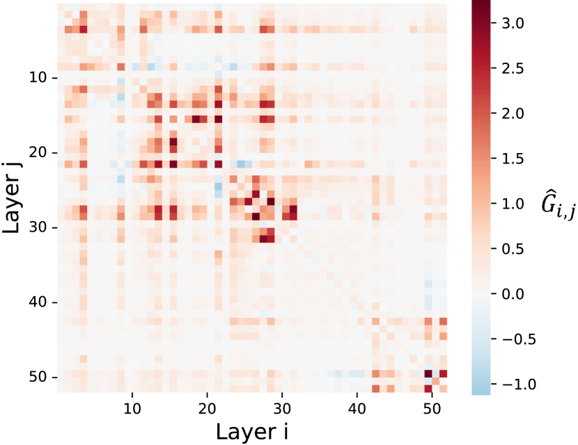
Figure 1: ResNet-50 on ImageNet: interactions between quantized layers on model performance are non-negligible. $[\hat{G}_{i,j}]$ is the sensitivity matrix that we define later by (10) in section 4.2, whose values are computed using (13) and (14).

A central claim of our work is that the assumption of layers’ independence and zero cross-layer dependency of error is inaccurate because interaction of quantization errors between layers exists empirically. Figure 1 illustrates the impact to model performance resulted from 2-bit quantization of ResNet-50 on ImageNet. We only quantize convolutional layers and each layer is assigned an unique index from 0 to 52. The diagonal terms $(i,i)$s show the increase in loss caused by quantizing a single layer $i$. The off-diagonal terms show the extra increase in loss due to quantizing a pair of layers $(i,j)$, compared to the sum of losses due to quantizing each layer alone. They capture the interaction of errors between layers. We observe that a non-negligible number of interactions have magnitudes comparable to diagonal terms. Moreover, the effect of interactions can be different when quantizing different sets of layers. Some of the interactions are destructive: they lead to extra increase in the sum of losses due to quantizing each layer alone, as indicated by the off-diagonal terms with positive values. Some others are helpful: they reduce the sum of losses, as indicated by the off-diagonal terms with negative values. However, all of these interactions are treated as negligible and ignored in prior sensitivity-based MPQ. Importantly, ignoring these cross-layer interactions leads to suboptimal MPQ solutions (see Section.3 for real-world cases of suboptimality with ResNet models on ImageNet classification).

To overcome this limitation of naive sensitivity-based MPQ, we propose CLADO (Cross-LAyer-Dependency-aware Optimization), an algorithm that measures the cross-layer dependency for all layers efficiently and optimizes a new cross-layer dependency aware objective via Integer Quadratic Programming (IQP). We start by applying the second-order Taylor expansion on network quantization loss. We decompose the loss into two components with each being a sum of terms. Terms in the first component are specific to individual layers and they act independently across layers. They are well-addressed in prior work and we refer to them as the layer-specific sensitivities. Terms in the second component, which prior work ignores, represent interactions between layers and we refer to them as the cross-layer sensitivities. Naively evaluating them requires calculation of inter-layer Hessian matrices, i.e., off-diagonal blocks of the network Hessian. However, direct computation of these matrices requires quadratic time and space complexity in the number of network parameters, which makes the computation practically infeasible. We propose an efficient backpropagation-free method that avoids Hessian calculation and computes sensitivities by solving a set of linear equations, that only require $O(L^{2})$ evaluations of network, on a small amount of data, to which we refer to as the sensitivity set. These sensitivities allow us to reformulate the original MPQ problem as an IQP that contains $O(L)$ binary variables and has linear constraints. The newly formulated IQP can be solved within seconds. The contributions of our work are:

• CLADO, a sensitivity-based algorithm that captures the cross-layer interactions of quantization error and transforms the MPQ problem into an Integer Quadratic Program that can be solved within seconds.

• CLADO is enabled by an efficient method to compute the cross-layer dependencies in $O(L^{2})$ time. It is backpropagation-free and only requires forward evaluations of DNNs on a small amount of training data.

• We present ablation studies that verify the importance of cross-layer dependencies in MPQ. Experiments on CNNs and transformer models show that CLADO achieves state-of-the-art mixed-precision quantization performance. E.g., on ImageNet, without finetuning, CLADO demonstrates an improvement, in top-1 classification accuracy, of up to $27\%$ over uniform precision quantization, and up to $15\%$ over existing MPQ methods; after finetuning, CLADO achieves $\leq 1\%$ degradation while other alternatives do not under several tight mode size constraints.

2 Prior Work

Existing mixed-precision quantization techniques can be divided into two classes: search-based and sensitivity-based.

Search methods evaluate the mixed-precision quantized networks’ performance and use it to guide the optimization process. HAQ Wang et al. (2019) and AutoQ Lou et al. (2020) use Reinforcement Learning (RL), where all possible bit-width assignments of layers are treated as the action space and the MPQ performance is interpreted as the reward. Other search methods, such as MPQDNAS Wu et al. (2018) and SPOS Guo et al. (2020), apply Neural Architecture Search (NAS) to make MPQ a differentiable search process. The advantage of these methods is that they make decisions based on explicit evaluation of the quantized model’s loss. However, they are computationally demanding, usually taking hundreds or even thousands of GPU-hours to complete Tang et al. (2022).

In contrast, sensitivity-based methods, use layer sensitivity as a proxy metric (or “critic”) to assess the impact of quantization on model performance. The sensitivities of layers in certain quantization precision are usually fast to measure, and once measured, they are reused in estimating the optimization objective as a function of different combinations of layer-wise precision assignments. This type of methods, including ZeroQ Cai et al. (2020), variants of HAWQ Dong et al. (2019, 2020) and MPQCO Chen et al. (2021), formulates the MPQ as a constrained combinatorial optimization problem. The objective to be minimized is the sum of layers’ sensitivities that quantify the overall quantization impact, while the constraints ensure certain target compression requirements, such as memory and/or computational budgets. (We note that there is also prior work, BRECQ Li et al. (2021), that defines sensitivities on blocks of adjacent layers. Except for the granularity of sensitivity measurement, this work shares the same methodologies as the above-described approach in formulating the MPQ as an optimization problem with its objective being the summation of sensitivities and its constraints being the compression requirement.) To measure the layers’ sensitivities, a small subset of training data is needed (e.g., $\sim 1024$ training samples for ImageNet). We refer to it as the sensitivity set. Different work defines sensitivities differently. Most of them use approximations to the Taylor expansion of network loss. Therefore, sensitivities defined in these work have theoretical implications to the increase in quantization loss. This line of work includes: Dong et al. (2019) uses the largest eigen value of ${H}_{w^{(l)}}$; Dong et al. (2020) uses the average trace of ${H}_{w^{(l)}}$; Chen et al. (2021) uses the Gauss-Newton Matrix. A few other work, e.g.,Cai et al. (2020), does not derive sensitivity from the Taylor expansion and have sensitivities defined with different physical meanings than the increase in quantization loss. The detailed formulas used by these work are presented in Table 1.

Since sensitivity-based methods optimize a proxy, instead of the real increase in network loss, they do not require iterative model evaluation and are efficient to solve. Recent work Chen et al. (2021) suggests that state-of-the-art sensitivity-based algorithms achieve performance comparable to that of search-based algorithms. Our proposed method CLADO is sensitivity-based.

Algorithm	Sensitivity $\Omega_{l}(\Delta w^{(l)})$	Notes on Notations
HAWQv1	$\sigma_{max}(H_{w^{(l)}})\cdot\left\|\Delta w^{(l)}\right\|_{2}^{2}$	$\sigma_{max}(H_{w^{(l)}})$: the largest singular
(Dong et al. (2019))		value of $l$-th layer’s Hessian
ZeroQ	$\sum_{j=1}^{N}\mathrm{KL}\left(f\left(w;x_{j}\right),f\left(w+\Delta w^{(l)};x_{j}\right)\right)$	KL($\cdot$): KL divergence function
(Cai et al. (2020))
HAWQv2/3	$\overline{\operatorname{Tr}}\left(H_{w^{(l)}}\right)\cdot\left\|\Delta w^{(l)}\right\|_{2}^{2}$	$\overline{\operatorname{Tr}}(H_{w^{(l)}})$: average of singular
(Yao et al. (2020))		values of $l$-th layer’s Hessian
MPQCO	$(\Delta w^{(l)})^{T}\tilde{H}_{w^{(l)}}\Delta w^{(l)}$	$\tilde{H}_{w^{(l)}}$: Gauss-Newton approx-
(Chen et al. (2021))		imation of $l$-th layer’s hessian

Table 1: Sensitivities (i.e., proxy of network loss) in prior work.

3 Cross-layer Dependency and MPQ Optimality

Empirically, cross-layer dependencies play non-negligible role in the search of optimal MPQ solutions and ignoring them may lead to suboptimal solutions. As for evidence, we present, on ImageNet, two examples of MPQ suboptimality caused by ignoring the cross-layer dependencies. To make the suboptimality easy to understand, we focus on only a few layers and assume that the problem is to choose two layers to quantize so that the quantization loss is minimized.

3.1 ResNet-34

Figure 2(a) shows the sensitivity matrix of ResNet-34 for 2-bit quantization on four layers: layer2.2.conv2 (index 12), layer3.1.conv2 (index 19), layer3.3.conv1 (index 22), and layer3.3.conv2 (index 23). The values are computed on 40k training samples. Ignoring the cross-layer interactions (off-diagonal terms) leads to the selection of layers $(12,19)$ because it gives the smallest predicted loss $0.115+0.140=0.255$. However, the real induced loss of quantizing layers $(12,19)$ is $0.115+0.140+2\times 0.009=0.273$ and the optimal solution is quantizing layers $(22,23)$ with the smallest induced loss $0.246+0.148+2\times(-0.070)=0.254$.

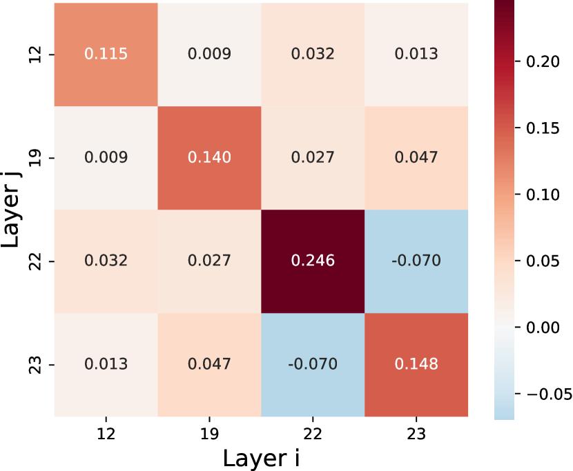
(a) ResNet-34

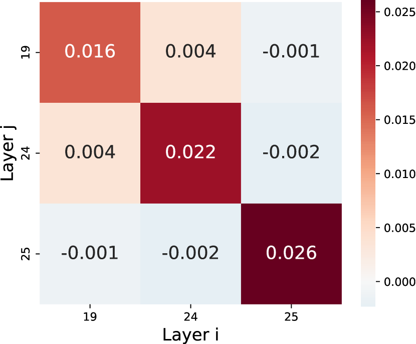
(b) ResNet-50

Figure 2: Sensitivity matrix of ResNet models. Entry $(i,i)$: increase in loss caused by quantizing a single layer $i$. Entry $(i,j)$: extra increase in loss due to quantizing a pair of layers $(i,j)$, compared to the sum of losses due to quantizing each layer alone.

3.2 ResNet-50

Figure 2(b) shows the sensitivity matrix of ResNet-50 for 4-bit quantization on three layers: they are layer2.2.conv3 (index 19), layer3.0.conv2 (index 24), and layer3.0.conv3 (index 25). Again, the values are computed on 40k training samples. Ignoring the cross-layer interactions leads to the selection of layers $(19,24)$ because it gives the smallest predicted loss $0.016+0.022=0.038$. However, the real induced loss is $0.038+2\times 0.004=0.046$. The optimal solution is quantizing layers $(19,25)$ with the smallest induced loss $0.016+0.026+2\times(-0.001)=0.040$.

4 Cross-LAyer-Dependency-aware Optimization (CLADO)

4.1 Preliminaries

We first introduce the notation and formulation of the MPQ problem following convention set in Chen et al. (2021).

Notation: We assume an $L$-layer (indices start from $0$) neural network $f:\mathbf{\Theta}\times\mathbb{X}\rightarrow\mathbb{Y}$ and a training dataset of $N$ samples $\left(\mathbf{x}^{(n)},\mathbf{y}^{(n)}\right)\in\mathbb{X}\times\mathbb{Y}$ with $n=\{1,\ldots,N\}$. The model maps each sample $\mathbf{x}^{(n)}$ to a prediction $\hat{\mathbf{y}}^{(n)}=f\left(\theta,\mathbf{x}^{(n)}\right)$, using some parameters $\theta\in\mathbf{\Theta}$. Then the predictions are compared with the ground truth $\mathbf{y}^{(n)}$ and evaluated with a task-specific loss function $\ell:\mathbb{Y}\times\mathbb{Y}\rightarrow\mathbb{R}$. For example, the cross-entropy loss is used for image classification. This leads to the objective function to minimize $\mathcal{L}:\mathbf{\Theta}\rightarrow\mathbb{R}$:

$$\mathcal{L}(\theta) =\frac{1}{N}\sum_{n=1}^{N}\ell\left(f\left(\theta,\mathbf{x}^{(n)}\right),\mathbf{y}^{(n)}\right)=\frac{1}{N}\sum_{n=1}^{N}\ell^{(n)}(\theta).$$ (1)

We denote the weight tensor of the $l^{th}$ layer as $W^{(l)}\in\mathbb{R}^{c_{o}\times c_{i}\times k\times k}$ and its flattened version as $w^{(l)}\in\mathbb{R}^{c_{o}c_{i}k^{2}}$, where $k$ is the kernel size for a convolutional layer and $k=1$ for fully-connected layers, $c_{i}$ and $c_{o}$ are the number of input and output channels, respectively. The quantization function is denoted by $Q:\mathbb{R}^{D}\times\mathbb{Z}^{+}\rightarrow\Pi_{b}$, which takes a full-precision vector and the quantization bit-width as input and produces the quantized vector. In this paper, we only consider uniform symmetric quantization as it is the most widely used scheme in practice due to its ease of implementation in hardware. As a result, $\Pi_{b}=s\times\left\{-2^{b-1},\ldots,0,\ldots,2^{b-1}-1\right\}$ for signed input and $s\times\left\{0,\ldots,2^{b}-1\right\}$ for unsigned one, where $b$ is the quantization bit-width and $s$ is the quantization scale factor. The quantized $b$-bit weight is given by $Q(w,b)=$ $\operatorname{clip}\left(\lfloor w/s\rceil,-2^{b-1},2^{b-1}-1\right)\times s$ for full precision $w$.

Discrete constrained optimization formulation: Let $w\triangleq\left\{w^{(l)}\right\}_{l=0}^{L-1}$ be the set of flattened weight tensors of the network. To find the optimal bit-width assignment with the goal of minimizing total model size, MPQ can be written as the following discrete constrained problem:

$$\begin{array}[]{c}\min_{\left\{b^{(l)}\right\}}\frac{1}{N}\sum_{n=1}^{N}\ell\left(f\left(w+\Delta w,\mathbf{x}^{(\mathbf{n})}\right),\mathbf{y}^{(\mathbf{n})}\right)\\ \text{ s.t. }\quad\Delta w^{(l)}=Q\left(w^{(l)},b^{(l)}\right)-w^{(l)}\\ \sum_{l}\left|w^{(l)}\right|\cdot b^{(l)}\leq C_{\text{target }}\\ b^{(l)}\in\mathbb{B}\\ l\in\{0,\ldots,L-1\},j\in\{1,\ldots,M\}\end{array}$$ (2)

$\mathbb{B}=\{b_{1},b_{2},...,b_{|\mathbb{B}|}\}$ denotes the set of bit-widths to be assigned in MPQ. In this work, $C_{\text{target }}$ is the target model size of the network, and $|\cdot|$ denotes the length of vectors.

Proxy of optimization objective: Let $g_{w}\triangleq\nabla\mathcal{L}(w)$ and $H_{w}\triangleq\nabla^{2}\mathcal{L}(w)$ be the gradient and the Hessian, respectively. For computational tractability, CLADO approximates the objective via the second-order Taylor expansion:

$$\mathcal{L}(w+\Delta w) =\frac{1}{N}\sum_{n=1}^{N}\ell^{(n)}(w+\Delta w)$$ (3)

$$\approx\mathcal{L}(w)+g_{w}^{T}\Delta w+\frac{1}{2}\Delta w^{T}H_{w}\Delta w.$$

For a well-trained model, it is reasonable to assume that training has converged to a local minimum, and thus, the gradient $g_{w}\approx 0$, resulting in:

$$\mathcal{L}(w+\Delta w)\approx\mathcal{L}(w)+\frac{1}{2}\Delta w^{T}H_{w}\Delta w.$$ (4)

In essence, MPQ seeks to minimize $\mathcal{L}(w+\Delta w)$ as a function of $\Delta w$, treating $\mathcal{L}(w)$ as a constant; thus, minimizing $\mathcal{L}(w+\Delta w)$ is equivalent to minimizing $\frac{1}{2}\Delta w^{T}H_{w}\Delta w$. Here we use $\Delta w^{T}H_{w}\Delta w$ as a proxy of the objective in (2).

4.2 Methods

The core of CLADO is a way to capture the interactions of error between layers that are ignored in prior work. We note that BRECQ Li et al. (2021) proposed a partial solution that addresses cross-layer dependencies for layers within a local block. However, BRECQ cannot be scaled to address cross-layer dependencies for all layers, because that will reduce it to an exhaustive search over $|\mathbb{B}|^{L}$ sensitivities, which is not computationally feasible. Importantly, we show that ignoring inter-block dependencies is sub-optimal in case of MPQ. CLADO presents the first sensitivity-based solution that addresses cross-layer dependencies for all layers.

Layer-specific and cross-layer sensitivities: Let $H_{ij}$s be the partition of the Hessian at layer-level granularity. Specifically, let $H_{ii}\triangleq{\partial^{2}\mathcal{L}(w)}/{\partial{w^{(i)}}^{2}}$ be the Hessian of layer $i$ and $H_{ij}\triangleq{\partial^{2}\mathcal{L}(w)}/{\partial w^{(i)}\partial w^{(j)}}$ be the cross-layer Hessian between layers $i$ and $j$. Unless otherwise stated, we use $i,j$ to denote the indices of layers and they take values from $\{0,1,..,L-1\}$. Then,

$$\Delta w^{T}H_{w}\Delta w=\sum_{i}\Delta w^{(i)T}H_{ii}\Delta w^{(i)}+\sum_{i\neq j}\Delta w^{(i)T}H_{ij}\Delta w^{(j)}$$ (5)

(5) decomposes the objective into two terms. The first term captures the contribution to loss increase from individual layers due to the intra-layer effects resulted from quantization. We refer to them as layer-specific sensitivities. The second part contains the contributions from effects of pairwise layer interaction as a consequence of two different layers being jointly quantized. We refer to them as the cross-layer sensitivties. We use $\Omega_{i,j}(\cdot,\cdot)$ as a unified notation for both types of sensitivities.

$$\Omega_{i,j}(\Delta w^{(i)},\Delta w^{(j)})\triangleq \Delta w^{(i)T}H_{ij}\Delta w^{(j)}$$ (6)

We rewrite (5) in terms of $\Omega$ as follows; minimizing (5) is equivalent to minimizing:

$$\Omega=\sum_{i}\Omega_{i,i}(\Delta w^{(i)},\Delta w^{(i)}) +\sum_{i\neq j}\Omega_{i,j}(\Delta w^{(i)},\Delta w^{(j)})$$ (7)

Note that this re-definition obviates direct reference to the Hessian. We will show below that $\Omega_{i,j}$ can be evaluated without computing the Hessian. Unlike prior work Dong et al. (2019); Cai et al. (2020); Dong et al. (2020); Chen et al. (2021) that ignores the cross-layer interaction terms, here we optimize (7) in its full form:

$$\begin{array}[]{c}\min_{\left\{b^{(l)}\right\}}\Omega\\ \text{ s.t. }\quad\Delta w^{(l)}=Q\left(w^{(l)},b^{(l)}\right)-w^{(l)}\\ \sum_{l}\left|w^{(l)}\right|\cdot b^{(l)}\leq C_{\text{target }}\\ b^{(l)}\in\mathbb{B}\\ l\in\{0,\ldots,L-1\}\end{array}$$ (8)

IQP formulation: Next we show that (8) can be formulated as an Integer Quadratic Program (IQP) that solves for the bit-width assignment decisions. Since each layer $l$ has $|\mathbb{B}|$ candidate bit-width choices:$\{b_{1},b_{2},..,b_{|\mathbb{B}|}\}$, $\Delta w^{(l)}$ can take $|\mathbb{B}|$ values: $\Delta w^{(l)}\in\{\Delta w^{(l)}_{1},\Delta w^{(l)}_{2},..,\Delta w^{(l)}_{|\mathbb{B}|}\}$. Here, we use $\Delta w^{(l)}_{m}\triangleq Q(w^{(l)},b_{m})-w^{(l)}$ with $m\in\{1,2,..,|\mathbb{B}|\}$ to denote the quantization error on $w^{(l)}$, when quantizing it to $b_{m}$ bits. For each layer $l$, we introduce a one-hot variable $\alpha^{(l)}\in\{0,1\}^{|\mathbb{B}|}\text{s.t.}\sum_{m=1}^{|\mathbb{B}|}\alpha_{m}^{(l)}=1$ to represent this layer’s bit-width decision. The single entry of $1$ in $\alpha^{(l)}$, e.g. $\alpha^{(l)}_{m}$, indicates the selection of a corresponding $\Delta w^{(l)}_{m}$ and the chosen bit-width $b_{m}$. For compact notation, let $\alpha\in\mathbb{R}^{|\mathbb{B}|L}$ be the concatenation of $\alpha^{(l)}s$. Specifically,

$$\alpha=(\alpha^{(0)},\alpha^{(1)},..\alpha^{(L-1)})$$ (9)

$$\Delta w^{(i)}=\alpha^{(i)}_{1}\Delta w^{(i)}_{1}+\alpha^{(i)}_{2}\Delta w^{(i)}_{2}+...+\alpha^{(i)}_{|\mathbb{B}|}\Delta w^{(i)}_{|\mathbb{B}|}$$

$$\Delta w^{(i)}_{m}=Q(w^{(i)},b_{m})-w^{(i)},\,m\in\{1,2,...,|\mathbb{B}|\}$$

$$\alpha^{(i)}_{1},\alpha^{(i)}_{2},...,\alpha^{(i)}_{|\mathbb{B}|}\in\{0,1\}$$

$$\alpha^{(i)}_{1}+\alpha^{(i)}_{2}+...+\alpha^{(i)}_{|\mathbb{B}|}=1$$

In addition, we gather all $\Omega_{i,j}$s into a matrix $\hat{G}\in\mathbb{R}^{|\mathbb{B}|L\times|\mathbb{B}|L}$, to which we refer to as the sensitivity matrix. Specifically, for $m,n\in\{1,2,..,|\mathbb{B}|\}$:

$$\hat{G}_{|\mathbb{B}|i+m,|\mathbb{B}|j+n}\triangleq\Omega_{i,j}(\Delta w^{(i)}_{m},\Delta w^{(j)}_{n})$$ (10)

Expand the $\Delta w^{(i)},\Delta w^{(j)}$ terms in (5) by (9) and bring in the definition of $\hat{G}$ in (10):

$$\Delta w^{T}H_{w}\Delta w=\sum_{i,j}\Delta w^{(i)T}H_{ij}\Delta w^{(j)}$$ (11)

$$= \sum_{i,j}(\sum_{m}\alpha^{(i)}_{m}\Delta w^{(i)T}_{m})H_{ij}(\sum_{n}\alpha^{(j)}_{n}\Delta w^{(j)}_{n})$$

$$= \sum_{i,j}\sum_{m}\sum_{n}\alpha^{(i)}_{m}\alpha^{(j)}_{n}\Delta w^{(i)T}_{m}H_{ij}\Delta w^{(j)}_{n}$$

$$= \sum_{i,j}\sum_{m}\sum_{n}\alpha^{(i)}_{m}\alpha^{(j)}_{n}\Omega_{i,j}(\Delta w^{(i)}_{m},\Delta w^{(j)}_{n})$$

$$= \sum_{i,j}\sum_{m}\sum_{n}\alpha_{|\mathbb{B}|i+m}\hat{G}_{|\mathbb{B}|i+m,|\mathbb{B}|j+n}\alpha_{|\mathbb{B}|j+n}$$

$$= \sum_{p=1}^{|\mathbb{B}|L}\sum_{q=1}^{|\mathbb{B}|L}\alpha_{p}\hat{G}_{p,q}\alpha_{q}=\alpha^{T}\hat{G}\alpha,$$

We have in (11) a rewritten objective $\Omega=\alpha^{T}\hat{G}\alpha$, in the form of a quadratic function in decision variables $\alpha$. Since $\hat{G}$ is a constant matrix composed of sensitivities, once these sensitivities are measured, the original MPQ problem can be reformulated as the following Integer Quadratic Program (IQP):

$$\begin{array}[]{c}\min_{\left\{\alpha^{(l)}\right\}}\alpha^{T}\hat{G}\alpha\\ \text{ s.t. }\alpha=(\alpha^{(1)},\alpha^{(2)},..\alpha^{(L)})\\ \alpha^{(l)}_{1},\alpha^{(l)}_{2},...,\alpha^{(l)}_{|\mathbb{B}|}\in\{0,1\}\\ \alpha^{(l)}_{1}+\alpha^{(l)}_{2}+...+\alpha^{(l)}_{|\mathbb{B}|}=1\\ \sum_{l}\sum_{m}\alpha^{(l)}_{m}\left|w^{(l)}\right|\cdot b_{m}\leq C_{\text{target }}\\ l\in\{0,\ldots,L-1\},\,\,m\in\{1,\ldots,|\mathbb{B}|\}\end{array}$$ (12)

Backpropagation-free sensitivity measurement: We now present an efficient way to compute $\hat{G}$ through only forward evaluations of DNNs. For any pair of layers $i,j$ and their corresponding bit-width choices $m,n$, computing $\Omega_{i}(\Delta w^{(i)}_{m})$, $\Omega_{j}(\Delta w^{(j)}_{n})$, and $\Omega_{i,j}(\Delta w^{(i)}_{m},\Delta w^{(j)}_{n})$ in a naïve manner requires computing the Hessians. Prior work, Dong et al. (2019, 2020); Chen et al. (2021), computes $\Omega_{i}(\Delta w^{(i)}_{m})$ and $\Omega_{i}(\Delta w^{(j)}_{n})$ through a bottom-up approach (again, it ignores $\Omega_{i,j}(\Delta w^{(i)}_{m},\Delta w^{(j)}_{n})$) by first approximating the Hessians and then the products.

However, we point out that there is no need to compute $\Omega$ explicitly under the assumption that the Taylor expansion (4) is a reasonable approximation of network loss, because $\Omega_{i,j}$s can be computed from the change in loss due to perturbation of individual layers’ parameters as follows:

$$\Omega_{i,i}(\Delta w^{(i)}_{m},\Delta w^{(i)}_{m})\approx 2\left(\mathcal{L}(w+\Delta w^{(i)}_{m})-\mathcal{L}(w)\right)$$ (13)

$$\Omega_{j,j}(\Delta w^{(j)}_{n},\Delta w^{(j)}_{n})\approx 2\left(\mathcal{L}(w+\Delta w^{(j)}_{n})-\mathcal{L}(w)\right)$$

$$\Omega_{i,i}(\Delta w^{(i)}_{m},\Delta w^{(i)}_{m})+\Omega_{j,j}(\Delta w^{(j)}_{n},\Delta w^{(j)}_{n})$$

$$+2\Omega_{i,j}(\Delta w^{(i)}_{m},\Delta w^{(j)}_{n})$$

$$\approx 2\left(\mathcal{L}(w+\Delta w^{(i)}_{m}+\Delta w^{(j)}_{n})-\mathcal{L}(w)\right).$$

The right sides of the three equations in (13) are computed by taking the difference in the loss of the quantized model from that of the full-precision model. Subtracting the first two equations from the third equation, we get:

$$\Omega_{i,j}(\Delta w^{(i)}_{m},\Delta w^{(j)}_{n})\approx\mathcal{L}(w+\Delta w^{(i)}_{m}+\Delta w^{(j)}_{n})+\mathcal{L}(w)$$ (14)

$$-\mathcal{L}(w+\Delta w^{(i)}_{m})-\mathcal{L}(w+\Delta w^{(j)}_{n}).$$

Importantly, (13) and (14) compute all sensitivities by only forward evaluations of DNNs on the small sensitivity set.

Positive semi-definite approximation: Instead of directly using the matrix $\hat{G}$, which is computed on the small sensitivity set, we first approximate it with a positive semi-definite (PSD) matrix. This is because, theoretically, $G$ is PSD if it is computed on the whole training set and the training has fully converged. However, since $\hat{G}$ is estimated by the sensitivity set that only contains a small number of training samples, the measurement error can make $\hat{G}$ indefinite. Practically, we find that the PSD approximation is critical to producing meaningful MPQ solutions, as it guarantees convexity of the IQP objective, making it much easier and faster to reach a good solution.

We provide a sketch of proof to show that $G$ is PSD. It uses proof by contradiction and starts by assuming that $G$ is not PSD. If $G$ is not PSD, then there exists a $v\in\mathbb{R}^{|\mathbb{B}|L}$ such that $v^{T}Gv<0$. Consider the following perturbation $u$ on weight:

$$u=(u_{0},\ldots,u_{L-1})\text{ with }u_{i}=\sum_{m=1}^{|\mathbb{B}|}v_{i|\mathbb{B}|+m}\Delta w^{(i)}_{m}$$ (15)

By using our definition of $G$ in (10), one can show that $u^{T}H_{w}u=v^{T}Gv$. We start by expanding $u^{T}H_{w}u$ in layer granularity ($i,j$ denote indices of layers and take values from $\{0,\ldots,L-1\}$; $m,n$ denote indices of bit-width options and take values from $\{1,\ldots,|\mathbb{B}|\}$). In the derivation, $(a)$ uses the definition of sensitivity (Equation 4.6); $(b)$ uses the definition of sensitivity matrix (Equation 4.10); $(c)$ is by introducing new variables $p,q$ with $p=|\mathbb{B}|i+m$ and $q=|\mathbb{B}|j+n$.

$$u^{T}H_{w}u=\sum_{i,j}u_{i}^{T}H_{ij}u_{j}$$ (16)

$$= \sum_{i,j}\left(\sum_{m}\Delta w^{(i)T}_{m}\right)H_{ij}\left(\sum_{n}\Delta w^{(j)}_{n}\right)$$

$$= \sum_{i,j}\sum_{m,n}v_{i|\mathbb{B}|+m}\left(\Delta w^{(i)T}_{m}H_{ij}\Delta w^{(j)}_{n}\right)v_{j|\mathbb{B}|+n}$$

$$\overset{(a)}{=} \sum_{i,j}\sum_{m,n}v_{i|\mathbb{B}|+m}\Omega_{i,j}(\Delta w_{m}^{(i)},\Delta w_{n}^{(j)})v_{j|\mathbb{B}|+n}$$

$$\overset{(b)}{=} \sum_{i,j}\sum_{m,n}v_{i|\mathbb{B}|+m}G_{|\mathbb{B}|i+m,|\mathbb{B}|j+n}v_{j|\mathbb{B}|+n}$$

$$\overset{(c)}{=} \sum_{p=1}^{|\mathbb{B}|L}\sum_{q=1}^{|\mathbb{B}|L}v_{p}G_{p,q}v_{q}=v^{T}Gv$$

Because of the equivalence between $v^{T}Gv$ and $u^{T}H_{w}u$, $u^{T}H_{w}u$ is negative according to the assumption that $G$ is not PSD. In consequence, by (4), $u$ forms a descending direction of loss and contradicts the fact that the network is trained to local optimal. Therefore, the assumption does not hold and $G$ must be PSD.

To apply PSD approximation on $\hat{G}$, one only needs to compute its eigen decomposition and replace the negative eigenvalues with zeros. We present in Algorithm 1 the complete CLADO algorithm. CLADO sensitivity computation requires $\frac{1}{2}|\mathbb{B}|L(|\mathbb{B}|L+1)$ measurements of the network on a small set of samples. Assuming measurements of DNN outputs take constant time complexity, CLADO has quadratic time complexity ($O(|\mathbb{B}|^{2}L^{2})$).

Algorithm 1 CLADO

Input: $L$-layer network with bit-width options $\mathbb{B}=\{b_{1},b_{2},..,b_{|\mathbb{B}|}\}$ and model size target $C_{\text{target}}$.

Output: The bit-width decision for each layer.

1:Evaluate the loss of full-precision model: $\mathcal{L}(w)$

2:Initialize $\hat{G}\in\mathbb{R}^{|\mathbb{B}|L\times|\mathbb{B}|L}$

3:for $i$ in $\{0,\ldots,L-1\}$ do

4:     for $m$ in $\{1,\ldots,|\mathbb{B}|\}$ do

5:         /* Quantize layer $i$ to $b_{m}$ bits

6:         $\Delta w^{(i)}\leftarrow Q(w^{(i)},b_{m})-w^{(i)}$

7:         /* Evaluate loss of quantized network

8:         Measure $\mathcal{L}(w+\Delta w^{(i)})$

9:         /* Compute layer-specific sensitivity

10:         $S\leftarrow 2\left(\mathcal{L}(w+\Delta w^{(i)})-\mathcal{L}(w)\right)$

11:         $\hat{G}_{|\mathbb{B}|i+m,|\mathbb{B}|i+m}\leftarrow S$

12:     end for

13:end for

14:for $i$ in $\{0,\ldots,L-2\}$ do

15:     for $j$ in $\{i+1,\ldots,L-1\}$ do

16:         for $(m,n)$ in $\{1,..|\mathbb{B}|\}\times\{1,..|\mathbb{B}|\}$ do

17:              /* Quantize layers $i$ and $j$ to $b_{m}$ and $b_{n}$ bits

18:              $\Delta w^{(i)}\leftarrow Q(w^{(i)},b_{m})-w^{(i)}$

19:              $\Delta w^{(j)}\leftarrow Q(w^{(j)},b_{n})-w^{(j)}$

20:              Evaluate $\mathcal{L}(w+\Delta w^{(i)}+\Delta w^{(j)})$

21:              /* Compute cross-layer sensitivities

22:              $S\leftarrow\mathcal{L}(w+\Delta w^{(i)}+\Delta w^{(j)})-\mathcal{L}(w)$

23:              $S\leftarrow S-0.5\hat{G}_{|\mathbb{B}|i+m,|\mathbb{B}|i+m}$

24:              $S\leftarrow S-0.5\hat{G}_{|\mathbb{B}|j+n,|\mathbb{B}|j+n}$

25:              $\hat{G}_{|\mathbb{B}|i+m,|\mathbb{B}|j+n}\leftarrow S$

26:         end for

27:     end for

28:end for

29:Compute the eigen-decomposition: $\hat{G}=\sum_{i=1}^{|\mathbb{B}|L}u_{i}e_{i}u_{i}^{T}$

30:Set PSD approximated $\hat{G}\leftarrow\sum_{i=1,e_{i}>0}^{|\mathbb{B}|L}u_{i}e_{i}u_{i}^{T}$

31:Solve the IQP problem in (12) by plugging in $\hat{G}$,$\mathbb{B}$, and $C_{\text{tagret}}$ to get the optimal solution $\alpha^{*}$.

32:Return the bit-width decisions indicated by $\alpha^{*}$.

5 Experimental Results: Convolutional Neural Networks

5.1 Experimental Settings

Dataset and models: We conduct experiments on the ImageNet dataset Russakovsky et al. (2014). To compare CLADO to existing work, we test two state-of-the-art algorithms: MPQCO Chen et al. (2021) and HAWQ-V3 Yao et al. (2020). We evaluate with four computer vision models: ResNet-34/50 He et al. (2015), RegNet-3.2GF Radosavovic et al. (2020), and MobileNetV3 Howard et al. (2019). For all models excluding MobileNetV3, we quantize activations to 8 bits and consider three candidate bit-widths for weights: $\mathbb{B}=\{2,4,8\}$. MobileNetV3, because of its compact architecture and high parameter efficiency, suffers higher degradation than other models at a constant compression ratio. For this reason, we consider more conservative quantization bit-width candidates with $\mathbb{B}=\{4,6,8\}$

Implementation details: All algorithms are implemented in PyTorch Paszke et al. (2019). The publicly available package CVXPY Diamond and Boyd (2016) is used to solve the IQP problem in CLADO and we select GUROBI Gurobi Optimization, LLC (2023) as its backend. For fair comparisons, all algorithms are run using the same procedures and settings. We download PyTorch pre-trained full-precision models. MQBench Li* et al. (2021) is applied for model quantization. Following prior work, quantization scale factors are determined by minimization of the MSE between the float32 values and their quantized values. This is achieved by setting the “weight observer” in MQBench to be MSEObserver.

Implementation Details: Our experiments are mainly conducted on a server equipped with a single Intel i7-9700 CPU, a single Nivida RTX2080 GPU, and 32GB DDR4 RAM.

Use of multiple sensitivity sets: To study the dependence of algorithms on the sensitivity set and to reduce the variation in results, we use multiple sensitivity sets. Specifically, for each sample size ranging from 256 to 4096, we randomly construct 24 sets with the given size. Then, we test the performance of algorithms on each of the 24 sets.

5.2 Code Implementations

We provide our code implementation of CLADO. We also include implementations of MPQCO and HAWQV3. Codes are zipped into a single file named codes.zip.

Structure of codes: Once unzipped, all codes including three Python files and one bash script are placed under the CLADO_SampleRun folder. prep_mpqco_clado.py computes the sensitivities for MPQCO and CLADO. prep_hawq.py computes the Hessian traces, which are used later by optimize.py to compute the sensitivities of HAWQ. optimize.py takes the pre-computed sensitivities (traces for HAWQ) and solves the corresponding IQP(for CLADO)/ILP(for HAWQ and MPQCO) problems to get the MPQ decisions. It then evaluates the decisions and report quantized models’ performance.

Dependencies: To run the codes, a CUDA environment with PyTorch, MQBench, Pyhessian, and CVXPY (with GUROBI backend) packages is required. We recommend to use PyTorch==1.10.1, MQBench==0.0.6, CVXPY==1.2.1, Pyhessian==0.1, and GUROBI-PY==9.5.2 to avoid any compatibility issues.

MPQ sample runs: sample_run.sh is an example script to run the experiments. It launches a quick run of three algorithms on the ResNet-34 model using a randomly sampled 64-sample sensitivity set. A datapath to the ImageNet dataset is required, it needs to be specified by user through the dp variable in the script. Once finished, one can check optimize.log for results. By default, we use bs=64 for batch size. The sb and eb define the indices of the starting and ending (inclusive) batches to be included in the sensitivity set (e.g., with the default batch size, one can specify sb=0,eb=15 to include 1024 samples in the sensitivity set). modelname specifies the model name of pretrained models by PyTorch, one can change it to other valid names (e.g., “resnet50”) listed in https://pytorch.org/vision/stable/models.html.

For other program arguments and hyperparameters, (e.g., CUDA device, number of threads, sampling of sensitivity samples, model size calculations and constraints), please see the codes for more details. Note that HAWQ uses Hutchinson’s method (via Pyhessian) to compute the Hessian traces, which is demanding of GPU memory. Therefore, when experimenting with deep models (e.g., ResNet-50), one may use a smaller batch size than 64 to avoid the OOM error.

Quantization settings: The quantization of models are handled by the MQBench package. The details of MQBench’s quantizer settings can be found in prep_mpqco_clado.py (line $154-181$). One can modify the MQBench settings there to test other settings of interest by specifying different hyperparameters including quantization granularity (per channel or per tensor), algorithms for quantization scale factors (MSE or Min-Max), formats of scale factors (power of two or continuous), etc.

Cached sensitivities: The sensitivities of algorithms are computed by prep_xxx.pys and are stored so that they can be reused for MPQ optimization with different constraints or additional analysis (e.g., for visualization of cross-layer interaction effects in Figures 2(a) and 2(b)). Specifically, sensitivities of CLADO are stored under folders named “Ltilde_xxx”; sensitivities of MPQCO are stored under folders named “DELTAL_xxx”; sensitivities and Hessian traces of HAWQ are stored under folders named “HAWQ_DELTAL_xxx”. The sensitivities are stored on a per-batch basis, with each representing the estimated sensitivities on a batch of training data (with batch size specified by bs). Note that these sensitivities (for all three algorithms) are additive across batches.

5.3 Comparison with Other MPQ Algorithms

Runtime: CLADO requires $\frac{1}{2}|\mathbb{B}|L(|\mathbb{B}|L+1)$ measurements of the network output on a small set of samples. On a single Nvidia RTX2080 GPU, our implementation takes 1 hour to generate the sensitivities for the ResNet-34 model and 2.5 hours to generate the sensitivities for the ResNet-50 model. HAWQ takes roughly the same number of GPU-hours as CLADO to perform the Hessian trace computation. MPQCO is the fastest one taking 5-10 minutes to compute the sensitivities. Further, the computation of sensitivity for CLADO can be parallelized by the use of multiple GPUs to further reduce the time (e.g., the use of 10 GPUs reduces the time by $10\times$). Search-based methods are several orders of magnitudes slower. They usually takes hundreds to thousands of GPU-hours to finish a search. Further, the search process cannot be easily parralelized because of the dependencies between the early and later search steps.

Average performance: Results of sensitivity-based algorithms depend on the size of the sensitivity set and show some variation. Figure 3 presents the averaged results of algorithms. In terms of average performance, CLADO delivers the best compressed models under most constraints. Its advantage over prior work is especially prominent when models are aggressively compressed to low precisions. Under the tightest size constraints tested, it achieves $9\%$ / $6\%$ higher top-1 accuracy than MPQCO/HAWQ on ResNet-34, $15\%$ / $7.5\%$ higher top-1 accuracy than MPQCO/HAWQ on ResNet-50, and $12.5\%$ / $8.5\%$ higher top-1 accuracy than MPQCO/HAWQ on RegNet-3.2GF. Under moderate compression requirements, e.g., $12-14$MB ResNet models and $8-11$MB RegNet models, performance drop of all algorithms is much smaller and hence smaller differences between algorithms. However, CLADO is still able to achieve, over the alternatives, $1-4\%$ higher top-1 accuracy on ResNet models, and around $1\%$ higher top-1 accuracy on RegNet-3.2GF. Under even higher model size constraints, all algorithms tend to be the same with the biggest difference in top-1 accuracy below $0.25\%$.

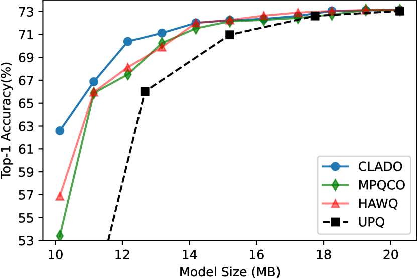
(a) ResNet-34

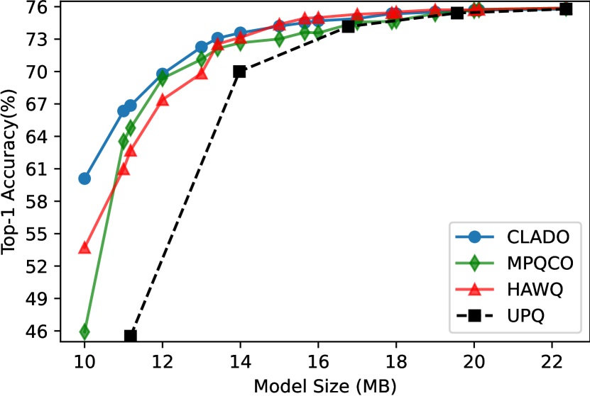
(b) ResNet-50

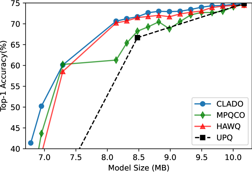
(c) RegNet-3.2GF

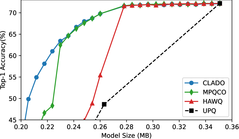
(d) MobileNetV3 Large

Figure 3: Model size vs. accuracy trade-off curves for CLADO, MPQCO, HAWQ, and UPQ. Data is the averaged accuracy on randomly-selected sensitivity sets.

Size of the sensitivity set: Figure 4 shows the median, the upper quartile (75%), and the lower quartile (25%) of algorithms’ performance on the randomly sampled sensitivity sets. CLADO produces reasonably stable results. Though it may have slightly higher variation than the alternatives, its lower quartile performance is almost always better than their upper quartile performance.

In addition, we found that CLADO keeps improving with larger sensitivity sets while MPQCO and HAWQ do not. Figure 5 shows, for RegNet, the change in algorithms’ average performance when using different sensitivity set sizes. When increasing the number of samples from 1024 to 4096, the performance of HAWQ and MPQCO either does not change at all or changes negligibly ($\approx 0.1\%$). However, CLADO’s performance improves by $0.58\%$, on average.

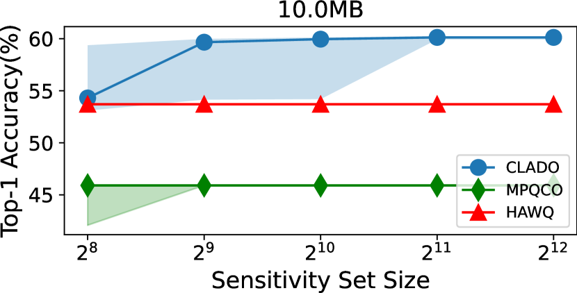
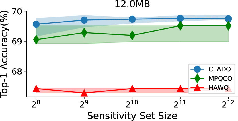
Figure 4: ResNet-50: dependence of different MPQs on the size of the sensitivity set. Data represents median accuracy on multiple randomly-selected sensitivity sets. Colored regions cover the upper and lower quartiles of accuracy for algorithms.

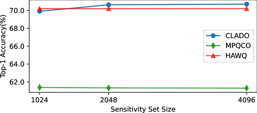
(a) 8.14MB

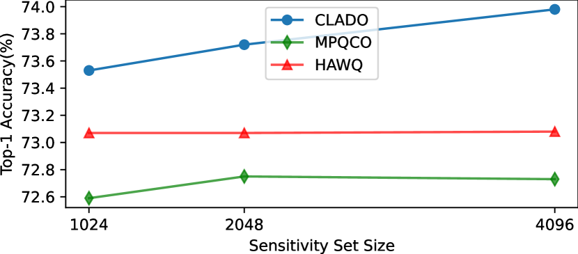
(b) 9.5MB

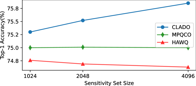
(c) 10.85MB

Figure 5: RegNet: dependence of different MPQs on the size of the sensitivity set. Data shows average accuracy. CLADO’s accuracy improves with more samples while models produced by MPQCO and HAWQ do not improve.

Analysis of bit-width assignments: Figures 7 and 6 visualize the MPQ decisions made by the three algorithms on ResNet-34 and ResNet-50, respectively. The other details and visualizations, including layer sensitivities measured by different methods and the proportion of parameters in each layer of the models, are included in Appendix.

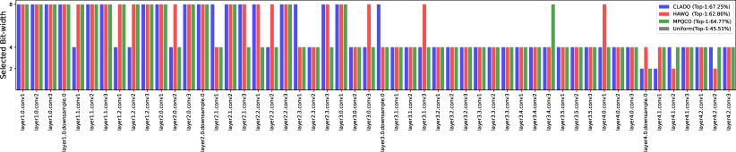
(a) 11.18MB

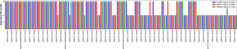
(b) 13.41MB

Figure 6: Bit-width assignments in ResNet-50.

All algorithms tend to assign more bits to shallow layers. This aligns with the observation that shallow layers have higher sensitivities and fewer parameters. In terms of sensitivity measurements, all methods agree that certain layers are very sensitive, e.g., the first down-sampling layer in the network. However, they can also differ significantly in predicting sensitivities of other layers. E.g., on both models, MPQCO predicts higher sensitivities for deep layers than other methods. For ResNet-50, HAWQ predicts much higher sensitivity for the first convolutional layer than other methods. The sensitivities measured by CLADO and the these measured by the KL-divergence appear closest in the shape of the distributions.

For all three methods, increasing the model size leads to monotonic increment of bit-width for each layer. Generally, layers with bigger sensitivities and smaller sizes tend to get larger bit-widths with higher priority than others. E.g., for CLADO and ResNet-34, from 8.87MB to 10.13MB (Figures 7(a) and 7(b)), there is a 6-bit bit-width increment to layer3.1.conv2 because this layer has high sensitivity and small size. In contrast, there is no bit-width increment for layer4.0.conv1 and layer4.0.conv2 because these layers are less sensitive and have more parameters. With the same change in model size, the three methods are very different in the change of their bit-width decisions. E.g., for ResNet-34 (Figure 7), from 8.87MB to 10.13MB, CLADO increases the bit-widths for 12 layers but HAWQ only increases the bit-widths for 4 layers; from 10.13MB to 12.16MB, the 6 layers whose bit-widths are increased by CLADO are completely different from the 8 layers whose bit-widths are increased by MPQCO.

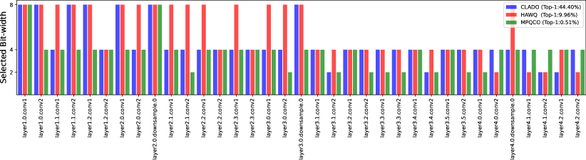
(a) 8.87MB

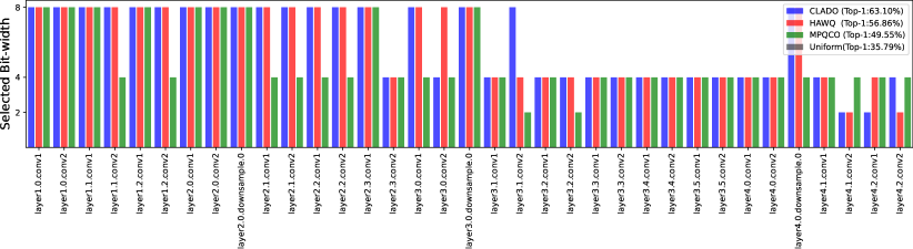
(b) 10.13MB

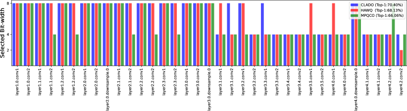
(c) 12.16MB

Figure 7: Bit-width assignments in ResNet-34.

5.4 MPQ Performance after Quantization-Aware Finetuning

So far, we studied MPQ in the post-training quantization (PTQ) settings, in which no further training is performed and only a small fraction of data is given (usually $\leq 1\%$ of the training data). However, if the whole training data and the access to the training pipeline are available, quantization-aware training/fine-tuning can be further applied. Such QAT tends to significantly reduce performance degradation.

To examine if CLADO’s bit-width assignments remain superior to others after fine-tuning, we conducted experiments of QAT fine-tunings applied on the mixed-precision quantized models produced by the three algorithms. We employ MQBench, the same quantization tool utilized in our previous experiments, to carry out the QAT experiments. We use batch size 32, SGD with learning rate $10^{-4}$ and the momentum of $0.9$. We found that CLADO’s bit-width assignments have faster QAT convergence at smaller losses than others, Figure 8. Most importantly, they maintain higher test performance than others after QAT, Figure 9. In the figure, PTQ results are not included because their accuracy is very low ($<45\%$) and they make the visualization of QAT difference difficult. Because QAT significantly reduces degradation, the difference between algorithms’ after-QAT performance is much smaller: for 8.87MB ResNet-34, CLADO, HAWQ, MPQCO achieve $44.40\%$, $9.96\%$, $0.51\%$ accuracy before QAT but after QAT, they achieve $72.34\%$, $72.00\%$, and $72.08\%$ accuracy, respectively. Although the after-QAT difference is small, CLADO maintains meaningful advantage: for ResNet-34 with 8.87MB size constraint and ResNet-50 with 8.94MB, 9.22MB, and 9.50MB constraints, CLADO achieves $\leq 1\%$ accuracy degradation but HAWQv3 and MPQCO do not.

(a) ResNet-34 (8.87MB).

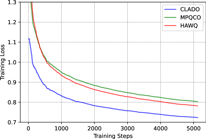
(b) ResNet-50 (8.38MB).

Figure 8: Training curve (finetuning): CLADO’s solutions have faster convergence to smaller losses.

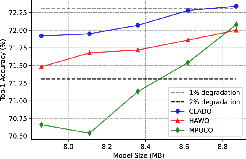
(a) ResNet-34 (FP Accuracy 73.31%)

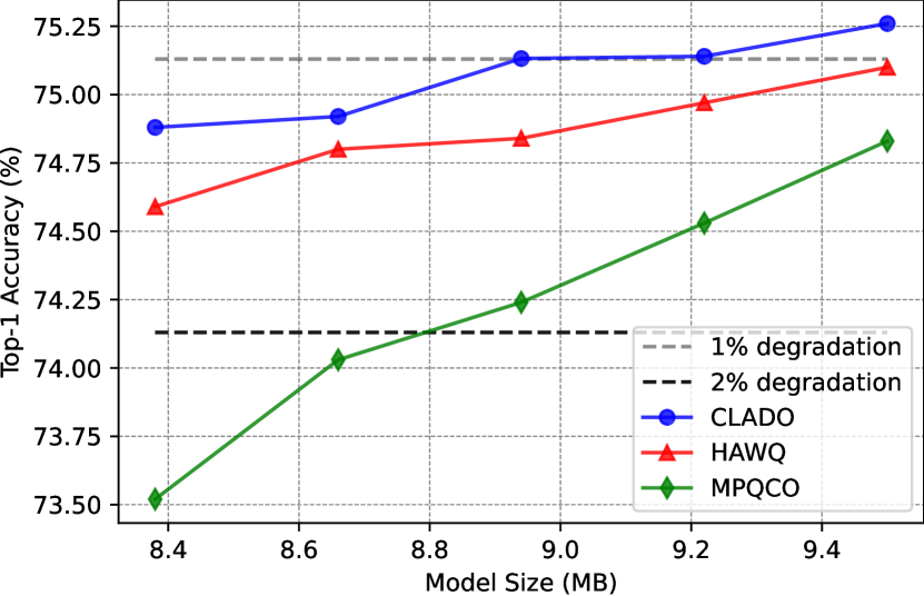
(b) ResNet-50 (FP Accuracy 76.13%)

Figure 9: Test accuracy after QAT: CLADO maintains higher performance.

5.5 Ablation Studies

We conduct ablation studies to justify the effectiveness and necessity of our method’s components.

Cross-Layer dependencies: To investigate the effectiveness of cross-layer dependencies, we test the performance of CLADO assuming zero cross-layer sensitivities. Specifically, we set $\hat{G}_{i,j}=0$ for $i\neq j$ and keep the rest of CLADO unchanged. We refer to this set of experiments as “Cross Removed”. Its results are captured by the orange curves in Figures 10 and 11. Comparing it with CLADO (blue curves), cross-layer dependencies improve MPQ performance and reduce algorithm’s variation, e.g., they lead to $7.5\%$ and $6\%$ increase in top-1 accuracy for 10.1MB ResNet-34 and 10MB ResNet-50, respectively.

We also conducted experiments in which cross-layer dependencies are only considered within blocks of layers, similar to BRECQ. In this set of experiments, we intentionally leave out the inter-block dependencies and keep the rest of CLADO unchanged. We refer to this group of experiments as “Block Interactions”. The results are captured by the black curves in Figure 12. We found that leaving out inter-block dependencies worsens MPQ compared to the CLADO (Full Interactions).

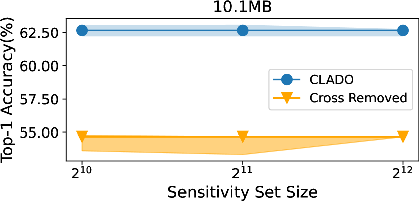
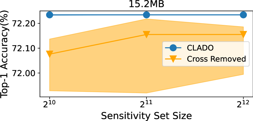
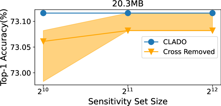
Figure 10: Ablation on Cross-layer Interactions: ResNet-34 on ImageNet

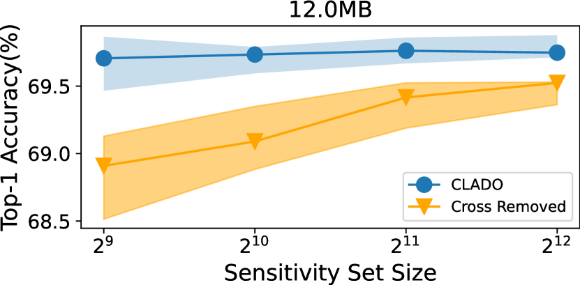
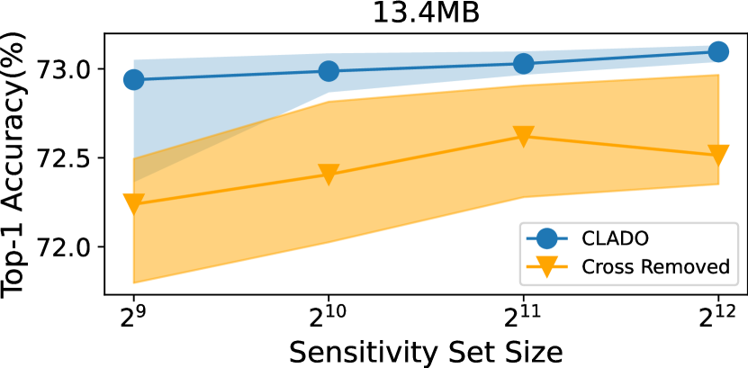
Figure 11: Ablation on Cross-layer Interactions: ResNet-50 on ImageNet

(a) ResNet-34: 10.14MB

(b) ResNet-34: 16.22MB

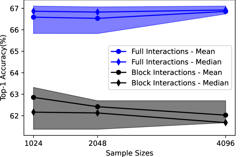
(c) ResNet-50: 11.18MB

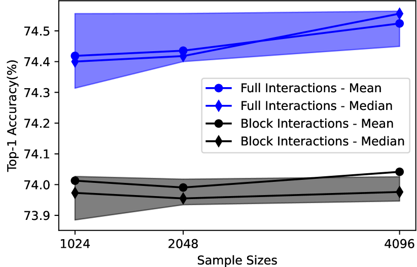
(d) ResNet-50: 15.65MB

Figure 12: Experiments confirm that leaving out inter-block dependencies worsens MPQ compared to CLADO. Blue: CLADO, captures all-layer dependencies. Black: intra-block dependency only, following BRECQ. 24 runs are launched using randomly sampled training data, the mean, median, upper quartile, and lower quartile performance are reported in the figure.

PSD approximation of sensitivity matrices: To investigate the effectiveness of PSD approximation, we disable the use of PSD approximation in CLADO, keeping the rest of CLADO unchanged. We found that, without the PSD approximation, it takes CVXPY indefinitely long to solve the IQP problem and reach only suboptimal solutions. With PSD approximation, the solver is able to compute the optimal solutions within seconds. This observation aligns with our expectation that using a convex objective $\Omega$ makes the IQP easy and efficient to solve. Its results are captured by the purple curves in Figures 13 and 14, we found that, though PSD does not always produce best results, it improves consistency in results and, in some cases, it prevents severe degradation in the quality of solutions, e.g., PSD improves the median top-1 accuracy, which is below $50\%$, to over $70\%$ for ResNet-50 under size constraints 13.4MB and 17.9MB.

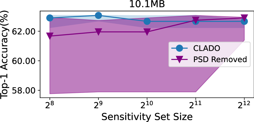
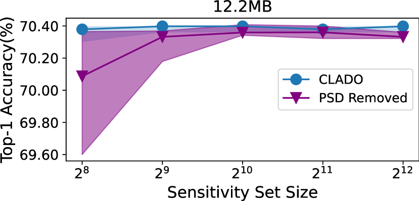
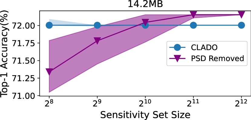
Figure 13: Ablation on PSD Approximation of Sensitivity Matrices: ResNet-34 on ImageNet

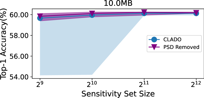
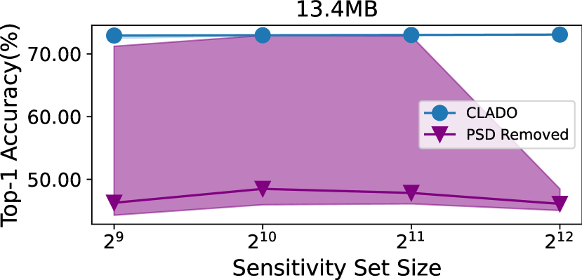
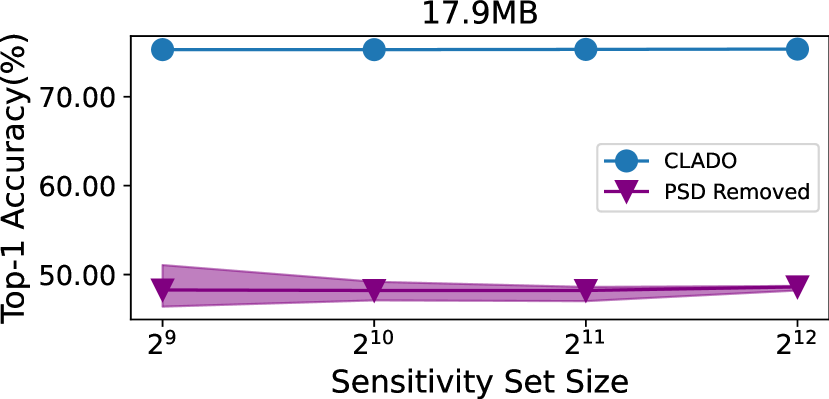
Figure 14: Ablation on PSD Approximation of Sensitivity Matrices: ResNet-50 on ImageNet

6 Experimental Results: Transformer-Based Models

Transformer-based models rely on attention mechanisms, which is powerful in processing long sequences of data tasks while addressing the limitations of Recurrent Neural Networks (RNNs) and Convolutional Neural Networks (CNNs). Recently, several transformer-based models Devlin et al. (2018); Dosovitskiy et al. (2020); Brown et al. (2020) have shown capability in advancing state-of-the-art performance in domains of NLP and CV. We choose two representative ones, ViT Dosovitskiy et al. (2020) for CV and BERT Devlin et al. (2018) for NLP, to verify the effectiveness of CLADO.

BERT (Bidirectional Encoder Representations from Transformers uses) Devlin et al. (2018) uses only the transformer encoder and learns deep bidirectional representations by jointly conditioning on both left and right context in all layers. This allows the model to pre-train on a large corpus of text and fine-tune for specific tasks, significantly improving the state-of-the-art for many NLP tasks. ViT (Vision Transformer) Dosovitskiy et al. (2020) applies the transformer architecture to image recognition tasks. It treats an image as a sequence of patches and applies self-attention and position embeddings on them, demonstrating that transformers can be used effectively for computer vision tasks. The pre-trained BERT base model is from HuggingFace library Wolf et al. (2020). We test it on the SQuAD dataset Rajpurkar et al. (2016). The pre-trained ViT is from PyTorch and we test it on the ImageNet dataset.

Figures 15(a) and 15(b) show the size/performance trade-offs for BERT and ViT, respectively. We found that while performance of other methods are task-dependent, CLADO always gives the best trade-offs. For example, on SQuAD, HAWQ achieves $\leq 2\%$ F1 score degradation when compressing the BERT model to 40MB while the degradation of MPQCO-quantized model is more than 10%; however, on ImageNet, MPQCO-quantized ViT is much better than HAWQ-quantized ViT: the performance gap, in terms of the top-1 accuracy, is more than 15% at model size 34MB. Though the improvements of CLADO over the best alternatives are small under large model sizes (40-80MB BERT,31-40MB ViT), they can be meaningful: on SQuAD, there is around 0.5% F1 score improvement for BERT with size 42.5-52.5MB; on ImageNet, there is 0.56% and 0.73% Top-1 accuracy improvement for ViT with size 31.44MB and 34.10MB, respectively. Under more restrictive settings, advantage of CLADO becomes bigger: for BERT with size constraint 37MB, CLADO achieves a F1 score of 82 while scores of HAWQ and MPQCO drop below 70; for ViT with size constraints 29.8MB and 28.2MB, CLADO achieves 5.64% higher and 21.82% higher accuracy than the best alternative.

By comparing the orange curves (CLADO with cross-layer terms set to 0) to others, we make the following observations. First, cross-layer interactions are helpful, but the degree of their helpfulness depends on the dataset and the model. In the experiments, improvements by considering cross-layer interactions are indicated by the performance lift from the orange curves to the blue curves (CLADO. Cross-layer interactions demonstrate greater improvements to the ViT model than to the BERT model: on ViT, they generally lead to $\geq 5\%$ improvement in Top-1 accuracy; on BERT, they translates into only $\sim 0.5\%$ F1 score improvement. Second, CLADO without cross-layer terms may achieve state-of-the-art performance in some tasks, but not all. For BERT on SQuAD, it is comparable to HAWQ: it is slightly worse than HAWQ (by $\leq 0.5\%$ Top-1 accuracy) under model sizes $\geq 50MB$ but is better than HAWQ (by $\geq 10\%$) under model size $<40MB$. However, for ViT on ImageNet, it is noticeably worse than MPQCO. Moreover, the fact that it is worse than MPQCO on ViT reduces the advantage of CLADO over MPQCO because the improvement due to cross-layer information is mitigated by a weaker baseline. As side notes to the above observations, there are two open questions that remain confusing and we leave for future research. They are, (1) why the degree of cross-layer interactions’ usefulness is task-dependent and (2) why the superiority of CLADO without cross-layer interactions over other methods are task-dependent.

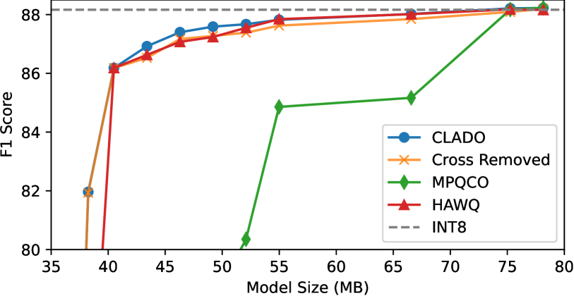
(a) BERT base on SQuAD

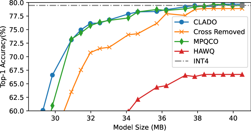
(b) ViT on ImageNet

Figure 15: Mixed-precision Quantization for Transformer-Based Models.

7 Conclusion

In this chapter, we present CLADO, the sensitivity-based mixed-precision quantization algorithm that exploits cross-layer quantization error dependencies. We use the second-order Taylor expansion on quantization loss to derive a proxy of optimization objective. While prior work ignores the cross-layer interaction terms, we propose to optimize the proxy in its full form and thereby reformulate the mixed-precision quantization as an integer quadratic programming problem that can be solved within seconds. To compute the cross-layer dependencies, we propose an efficient approach based on the Taylor expansion, which requires only forward evaluations of DNNs on the small sensitivity set. Extensive experiments are conducted to demonstrate the effectiveness of the proposed method over the uniform precision quantization and other mixed-precision quantization approaches.

Appendix A Appendix: Layer Sensitivities of ResNet Models Measured by Different Methods

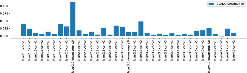
(a) CLADO

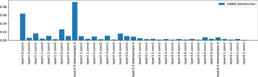
(b) HAWQ

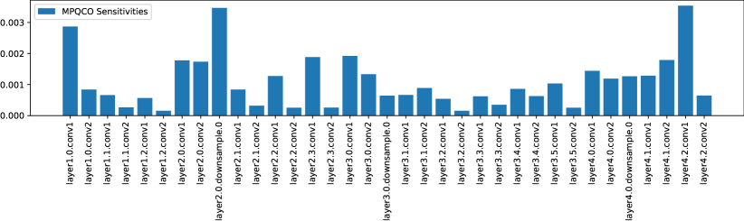
(c) MPQCO

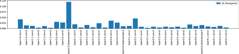
(d) KL-Divergence

Figure 16: Sensitivities of ResNet-34 layers measured by different methods.

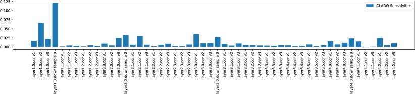
(a) CLADO

(b) HAWQ

(c) MPQCO

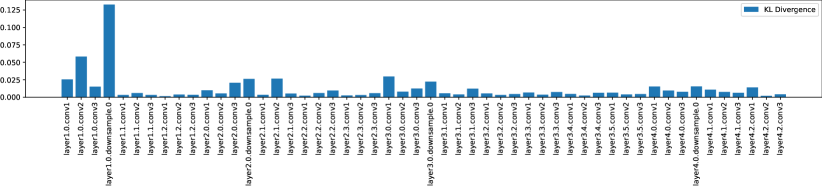
(d) KL-Divergence

Figure 17: Sensitivities of ResNet-50 layers measured by different methods.

Appendix B Appendix: Proportion of Parameters for Each Layer in ResNet Models

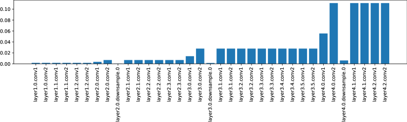
Figure 18: Proportion of parameters for each layer in ResNet-34.

Figure 19: Proportion of parameters for each layer in ResNet-50.

References

- Courbariaux et al. [2015] Matthieu Courbariaux, Yoshua Bengio, and J. David. Binaryconnect: Training deep neural networks with binary weights during propagations. In NIPS, 2015.
- Nagel et al. [2020] Markus Nagel, Rana Ali Amjad, Mart van Baalen, Christos Louizos, and Tijmen Blankevoort. Up or down? adaptive rounding for post-training quantization. ArXiv, abs/2004.10568, 2020.
- Kim et al. [2021] Sehoon Kim, Amir Gholami, Zhewei Yao, Michael W. Mahoney, and Kurt Keutzer. I-bert: Integer-only bert quantization. ArXiv, abs/2101.01321, 2021.
- Wei et al. [2022] Xiuying Wei, Ruihao Gong, Yuhang Li, Xianglong Liu, and Fengwei Yu. Qdrop: Randomly dropping quantization for extremely low-bit post-training quantization. ArXiv, abs/2203.05740, 2022.
- Deng and Orshansky [2022] Zihao Deng and Michael Orshansky. Variability-aware training and self-tuning of highly quantized dnns for analog pim. 2022 Design, Automation & Test in Europe Conference & Exhibition (DATE), pages 712–717, 2022.
- Nagel et al. [2021] Markus Nagel, Marios Fournarakis, Rana Ali Amjad, Yelysei Bondarenko, Mart van Baalen, and Tijmen Blankevoort. A white paper on neural network quantization. ArXiv, abs/2106.08295, 2021.
- Hubara et al. [2021] Itay Hubara, Yury Nahshan, Yair Hanani, Ron Banner, and Daniel Soudry. Accurate post training quantization with small calibration sets. In ICML, 2021.
- Cai et al. [2020] Yaohui Cai, Zhewei Yao, Zhen Dong, Amir Gholami, Michael W. Mahoney, and Kurt Keutzer. Zeroq: A novel zero shot quantization framework. 2020 IEEE/CVF Conference on Computer Vision and Pattern Recognition (CVPR), pages 13166–13175, 2020.
- Dong et al. [2019] Zhen Dong, Zhewei Yao, Amir Gholami, Michael W. Mahoney, and Kurt Keutzer. Hawq: Hessian aware quantization of neural networks with mixed-precision. 2019 IEEE/CVF International Conference on Computer Vision (ICCV), pages 293–302, 2019.
- Yang and Jin [2020] Linjie Yang and Qing Jin. Fracbits: Mixed precision quantization via fractional bit-widths. In AAAI Conference on Artificial Intelligence, 2020.
- Tang et al. [2022] Chen Tang, Kai Ouyang, Zhi Wang, Yifei Zhu, Yao Wang, Wen Ji, and Wenwu Zhu. Mixed-precision neural network quantization via learned layer-wise importance. ArXiv, abs/2203.08368, 2022.
- Wang et al. [2019] Kuan Wang, Zhijian Liu, Yujun Lin, Ji Lin, and Song Han. Haq: Hardware-aware automated quantization with mixed precision. 2019 IEEE/CVF Conference on Computer Vision and Pattern Recognition (CVPR), pages 8604–8612, 2019.
- Lou et al. [2020] Qian Lou, Feng Guo, Lantao Liu, Minje Kim, and Lei Jiang. Autoq: Automated kernel-wise neural network quantization. arXiv: Learning, 2020.
- Wu et al. [2018] Bichen Wu, Yanghan Wang, Peizhao Zhang, Yuandong Tian, Péter Vajda, and Kurt Keutzer. Mixed precision quantization of convnets via differentiable neural architecture search. ArXiv, abs/1812.00090, 2018.
- Guo et al. [2020] Zichao Guo, Xiangyu Zhang, Haoyuan Mu, Wen Heng, Zechun Liu, Yichen Wei, and Jian Sun. Single path one-shot neural architecture search with uniform sampling. In ECCV, 2020.
- Dong et al. [2020] Zhen Dong, Zhewei Yao, Yaohui Cai, Daiyaan Arfeen, Amir Gholami, Michael W. Mahoney, and Kurt Keutzer. Hawq-v2: Hessian aware trace-weighted quantization of neural networks. ArXiv, abs/1911.03852, 2020.
- Chen et al. [2021] Weihan Chen, Peisong Wang, and Jian Cheng. Towards mixed-precision quantization of neural networks via constrained optimization. 2021 IEEE/CVF International Conference on Computer Vision (ICCV), pages 5330–5339, 2021.
- Yao et al. [2020] Zhewei Yao, Zhen Dong, Zhangcheng Zheng, Amir Gholami, Jiali Yu, Eric Tan, Leyuan Wang, Qijing Huang, Yida Wang, Michael W. Mahoney, and Kurt Keutzer. Hawqv3: Dyadic neural network quantization. In International Conference on Machine Learning, 2020.
- Li et al. [2021] Yuhang Li, Ruihao Gong, Xu Tan, Yang Yang, Peng Hu, Qi Zhang, Fengwei Yu, Wei Wang, and Shi Gu. Brecq: Pushing the limit of post-training quantization by block reconstruction. ArXiv, abs/2102.05426, 2021.
- Russakovsky et al. [2014] Olga Russakovsky, Jia Deng, Hao Su, Jonathan Krause, Sanjeev Satheesh, Sean Ma, Zhiheng Huang, Andrej Karpathy, Aditya Khosla, Michael S. Bernstein, Alexander C. Berg, and Li Fei-Fei. Imagenet large scale visual recognition challenge. International Journal of Computer Vision, 115:211–252, 2014.
- He et al. [2015] Kaiming He, X. Zhang, Shaoqing Ren, and Jian Sun. Deep residual learning for image recognition. 2016 IEEE Conference on Computer Vision and Pattern Recognition (CVPR), pages 770–778, 2015.
- Radosavovic et al. [2020] Ilija Radosavovic, Raj Prateek Kosaraju, Ross B. Girshick, Kaiming He, and Piotr Dollár. Designing network design spaces. 2020 IEEE/CVF Conference on Computer Vision and Pattern Recognition (CVPR), pages 10425–10433, 2020.
- Howard et al. [2019] Andrew G. Howard, Mark Sandler, Grace Chu, Liang-Chieh Chen, Bo Chen, Mingxing Tan, Weijun Wang, Yukun Zhu, Ruoming Pang, Vijay Vasudevan, Quoc V. Le, and Hartwig Adam. Searching for mobilenetv3. 2019 IEEE/CVF International Conference on Computer Vision (ICCV), pages 1314–1324, 2019.
- Paszke et al. [2019] Adam Paszke, Sam Gross, Francisco Massa, Adam Lerer, James Bradbury, Gregory Chanan, Trevor Killeen, Zeming Lin, Natalia Gimelshein, Luca Antiga, Alban Desmaison, Andreas Köpf, Edward Yang, Zach DeVito, Martin Raison, Alykhan Tejani, Sasank Chilamkurthy, Benoit Steiner, Lu Fang, Junjie Bai, and Soumith Chintala. Pytorch: An imperative style, high-performance deep learning library. In Neural Information Processing Systems, 2019.
- Diamond and Boyd [2016] Steven Diamond and Stephen P. Boyd. Cvxpy: A python-embedded modeling language for convex optimization. Journal of machine learning research : JMLR, 17, 2016.
- Gurobi Optimization, LLC [2023] Gurobi Optimization, LLC. Gurobi Optimizer Reference Manual, 2023. URL https://www.gurobi.com.
- Li* et al. [2021] Yuhang Li*, Mingzhu Shen*, Jian Ma*, Yan Ren*, Mingxin Zhao*, Qi Zhang*, Ruihao Gong*, Fengwei Yu, and Junjie Yan. Mqbench: Towards reproducible and deployable model quantization benchmark. Proceedings of the Neural Information Processing Systems Track on Datasets and Benchmarks, 2021.
- Devlin et al. [2018] Jacob Devlin, Ming-Wei Chang, Kenton Lee, and Kristina Toutanova. Bert: Pre-training of deep bidirectional transformers for language understanding. arXiv preprint arXiv:1810.04805, 2018.
- Dosovitskiy et al. [2020] Alexey Dosovitskiy, Lucas Beyer, Alexander Kolesnikov, Dirk Weissenborn, Xiaohua Zhai, Thomas Unterthiner, Mostafa Dehghani, Matthias Minderer, Georg Heigold, Sylvain Gelly, Jakob Uszkoreit, and Neil Houlsby. An image is worth 16x16 words: Transformers for image recognition at scale. arXiv preprint arXiv:2010.11929, 2020.
- Brown et al. [2020] Tom B Brown, Benjamin Mann, Nick Ryder, Melanie Subbiah, Jared Kaplan, Prafulla Dhariwal, Arvind Neelakantan, Pranav Shyam, Girish Sastry, Amanda Askell, et al. Language models are few-shot learners. arXiv preprint arXiv:2005.14165, 2020.
- Wolf et al. [2020] Thomas Wolf, Lysandre Debut, Victor Sanh, Julien Chaumond, Clement Delangue, Anthony Moi, Pierric Cistac, Tim Rault, Rémi Louf, Morgan Funtowicz, Joe Davison, Sam Shleifer, Patrick von Platen, Clara Ma, Yacine Jernite, Julien Plu, Canwen Xu, Teven Le Scao, Sylvain Gugger, Mariama Drame, Quentin Lhoest, and Alexander Rush. Transformers: State-of-the-art natural language processing, 2020.
-
Rajpurkar et al. [2016]
Pranav Rajpurkar, Jian Zhang, Konstantin Lopyrev, and Percy Liang.
Squad: 100,000+ questions for machine comprehension of text.
arXiv preprint arXiv:1606.05250, 2016.