Learning Active Subspaces and Discovering Important Features with Gaussian Radial Basis Functions Neural Networks

Abstract

Providing a model that achieves a strong predictive performance and at the same time is interpretable by humans is one of the most difficult challenges in machine learning research due to the conflicting nature of these two objectives. To address this challenge, we propose a modification of the Radial Basis Function Neural Network model by equipping its Gaussian kernel with a learnable precision matrix. We show that precious information is contained in the spectrum of the precision matrix that can be extracted once the training of the model is completed. In particular, the eigenvectors explain the directions of maximum sensitivity of the model revealing the active subspace and suggesting potential applications for supervised dimensionality reduction. At the same time, the eigenvectors highlight the relationship in terms of absolute variation between the input and the latent variables, thereby allowing us to extract a ranking of the input variables based on their importance to the prediction task enhancing the model interpretability. We conducted numerical experiments for regression, classification, and feature selection tasks, comparing our model against popular machine learning models and the state-of-the-art deep learning-based embedding feature selection techniques. Our results demonstrate that the proposed model does not only yield an attractive prediction performance with respect to the competitors but also provides meaningful and interpretable results that potentially could assist the decision-making process in real-world applications. A PyTorch implementation of the model is available on GitHub at the following link.

1 Introduction

The Radial Basis Function (RBF) is a family of models used for function interpolation and approximation that are defined as a linear combination of radially symmetric basis functions broomhead1988radial . The RBF approach has many properties which make it attractive as a mathematical tool for interpolation micchelli1984interpolation ; powell2001radial . Once the basis function and its hyperparameters are determined, the weights that multiply the basis functions can be found by solving a convex optimization problem or directly through matrix inversion. The RBF model has been generalized in the context of approximation by using basis functions centered with respect to a subset of the data, that can be interpreted as one hidden layer Neural Network (RBF-NN) with RBF’s activation function as shown in broomhead1988radial . In park1991universal ; park1993approximation the authors showed that under some conditions on the basis function, RBF-NNs are universal approximators as Neural Networks (NNs) hornik1989multilayer .

Radial Basis Functions have been used for function interpolation or approximation for many decades in different applications. In the work presented in poggio1990networks ; girosi1995regularization the authors showed that from the regularization principles and through a solution of a variational problem, the RBF model is a subclass of regularization networks. Particularly important, in the case of the Gaussian RBF (GRBF), is the definition of the shape parameter bishop1995neural , which is problem dependent and controls the variance (or the width) of the Gaussian basis function. The GRBF is very sensitive to the shape parameter as shown empirically in mongillo2011choosing in case of interpolation, and a usual way to set it is to fix it through cross-validation procedures.

In general, various methods have been proposed to estimate the parameters of RBF-NNs in the context of approximation. Some of them are inspired by the work presented in poggio1990networks where the location of the centers and a weighted norm (instead of the classical Euclidean norm) are considered part of the learning problem together with the weights. The possibility to use a superposition of kernels with a distinct set of hyperparameters has been also considered poggio1990networks . In moody1989fast they propose to compute the width factors by the nearest neighbors heuristic and a clustering procedure for the centers. A different approach has been used in wettschereck1991improving , where the centers’ locations are considered as additional parameters of the optimization problem as well as the weights. In the same work, they also considered learning the width of the Gaussian kernel around each center, but this hurt the generalization performance of the model wettschereck1991improving . A similar approach has been presented in schwenker2001three where a diagonal precision matrix is also considered for each RBF center. Important research to improve the generalization power of RBF-NNs is in bishop1991improving . This has been achieved by adding a regularization term that penalizes the second derivative of the output of each neuron. The technique is also known in the case of NNs in bishop1992curvature .

As in the case of NNs, RBF-NNs are considered as black-box models, and consequently, the underlying process of how the input features are used to make predictions is not clear to humans, including those who developed the models. For this reason, sometimes simpler models given just by a linear combination of the input variables are preferred since the coefficients can give an assessment of the importance of each feature in the prediction task. On the other hand, simpler models tend to be less accurate than complex ones. As a result, it is crucial to propose models with powerful predictive capabilities that can also provide simple explanations to support decision-making in complex real-world applications. Thus, recognizing the importance of each input feature in a prediction task from a machine learning model has significant implications in various fields, including genomics bi2020interpretable , environmental science dikshit2021interpretable , emergency medicine wong2022development , cancer research hauser2022explainable , and finance ohana2021explainable . In these domains, the model interpretability is crucial as the predictive performance as described in guidotti2018survey ; arrieta2020explainable ; adadi2018peeking .

Explainable AI (XAI) is a rapidly growing field of research that aims to make AI models more transparent and interpretable to humans. XAI techniques provide insight into the decision-making processes of AI models, allowing users to understand how models arrive at their outputs and to identify potential biases or errors. Feature importance ranking (FIR) and feature selection (FS) are two key techniques used in XAI. FIR involves evaluating the contribution of each feature to the output of a model, allowing users to identify which features are most important in driving the model predictions. FS involves choosing a subset of features that are most relevant to the model predictions, which can improve model performance due to the curse of dimensionality bellman1966dynamic .

According to the taxonomy in guyon2003introduction there are three kinds of feature selection methods: filter, wrapper, and embedded. Filter methods for feature selection are techniques that use statistical measures to rank the importance of each feature independently of the model, such as Chi-squared feature selection and variance thresholding. These methods are called "filter" because they filter out irrelevant or redundant features from the dataset before the learning algorithm is applied. Wrapper methods work by selecting a subset of features, training the learning algorithm on that subset, evaluating its performance using cross-validation, and then repeating the process with different feature subsets. This iterative approach can be time-consuming and inefficient. A popular wrapper method is the forward/backward feature elimination hastie2009elements . Embedded methods refer to learning algorithms that have FS incorporated. Embedded methods are optimal and time-efficient because they use the target learning algorithm in the selection of features. Some of the embedded methods are linear models such as the LASSO regression tibshirani2011regression , and tree-based methods such as the Random Forest (RF) breiman2001random and Gradient Boosting (GB) friedman2001greedy . They are inherently easier to interpret and have become prevalent tools across practitioners. Recently, Deep Feature Selection (DFS) li2016deep and the approach proposed in wojtas2020feature highlight the important features of NNs architectures. An emerging new kind of feature selection methods are the post-hoc explanators such as SHAP (SHapleyAdditive exPlanations) lundberg2017unified and LIME (Local Interpretable Model-agnostic Explanations) ribeiro2016should . They are applied after the model has made its predictions and provide insights into why the model has made a certain decision.

In parallel to XAI, to make accurate predictions, it is important for models to extract only the salient features from the data and act as feature extractors. One approach to achieving this is through the discovery of underlying factors of variation that generated the data, which may live in a subspace of much lower dimensionality than the input space. As an example, the success of deep learning models has been also imputed to their capability to learn and exploit latent representations through a cascade of multiple non-linear transformations of the dataset bengio2013representation . From an unsupervised learning perspective, the popular Principal Component Analysis (PCA) pearson1901liii ; hotelling1933analysis can be used to prune out irrelevant directions in the data, constructing a latent space given as a linear combination of independent factors. In supervised learning, the Fisher linear discriminant fisher1936use learns a new reduced representation taking into account the classification task by searching for those vectors in the latent space that best discriminate among classes. In the context of statistical regression, there is also a vast body of literature about methods for finding a low-dimensional subspace of the input feature space that is statistically sufficient to characterize the input feature/response relationship known as sufficient dimension reduction (SDR) adragni2009sufficient ; cook2009regression ; cook1994interpretation and effective dimension reduction (EDR) li1991sliced . These methodologies are closely related to the concept of active subspace.

The Active Subspace Method (ASM) constantine2014active , can be used to discover directions of maximum variability of a particular function by applying a PCA to a dataset composed of its gradients. By eliminating directions defined by the eigenvectors associated with zero eigenvalues one can provide a reduced representation (i.e. the active subspace) where most of the original function variability is preserved. The ASM showed to be relevant in many areas of science and engineering such as in hydrology jefferson2015active , shape optimization lukaczyk2014active , and disease modeling loudon2016mathematical . It enables efficient exploration of the model input space and can help reduce computational costs associated with sensitivity analysis, uncertainty quantification, and optimization.

2 Main contribution

This paper presents modifications to the classical RBF model, focusing specifically on Gaussian RBF Neural Networks (GRBF-NNs) for function approximation.

Our main contribution is to enhance the interpretability of the model while maintaining the excellent predictive performance of RBF-NN architectures. This is achieved by exploiting latent relationships between input features and the response variable, highlighting the factors of variation in the data, revealing the active subspace, and identifying the input variables that played prominent roles in the learning task. To achieve this, we equip the kernel of the model with a learnable symmetric precision matrix. The latent information about the prediction task can be extracted by analyzing the spectrum of the precision matrix once the training of the model has been completed. The eigenvalues provide valuable information regarding the second derivative of the argument of the Gaussian kernel at the GRBF-NN centers. Dominant eigenvalues correspond to eigenvectors that explain a significant portion of the variability within the GRBF-NN model. Therefore, analyzing these eigenvalues allows us to understand the directions in which the GRBF-NN model exhibits the most variability. Consequently, one can use our proposed model for supervised dimensionality reduction purposes, for example by projecting the overall learning task in a 2-dimensional active subspace for visualization.

In parallel, to make our model more transparent and interpretable to humans, we estimate the FIR of the learning task allowing one to use our model for FS purposes. This can be easily achieved by knowing that the eigenvectors also represent the Jacobian of the linear transformation of a new coordinate system defined in the latent space. This means that we can assess how a change in a particular latent variable affects the input variables thereby assessing the importance of the input feature for the current prediction task.

To improve the smoothness and the generalization capability of our model, we introduce two regularization parameters: one for the weights and the other one for the elements of the precision matrix of the Gaussian kernel. To better analyze the behavior of our model, we investigate the synergy between them. Interestingly, numerical results suggest that a stronger role is played by the regularizer of the precision matrix rather than the one that controls the magnitude of the weights.

In the end, we conduct numerical experiments to compare our proposed model with other popular machine learning models such as SVM’s cortes1995support , Random Forest (RF) breiman2001random , Gradient Boosting (GB) friedman2001greedy , and state-of-the-art deep learning embedding methods such as the ones presented in li2016deep ; wojtas2020feature . The results show that our model not only achieves competitive prediction performances but also provides meaningful and interpretable insights.

3 Model Description

Radial Basis Functions have been introduced for solving interpolation problems, which consist of building the following interpolant

$$f(\mathbf{x})=\sum_{m=1}^{M}w_{m}\varphi(||\mathbf{x}-\mathbf{x}_{m}||)$$ (1)

where we have $M$ weights $w_{m}\in\mathbb{R}$, a continuous function $\varphi:\mathbb{R}^{+}\rightarrow\mathbb{R}$ which represents the basis function, and the centers $\mathbf{x}_{m}$. One can solve the interpolation problem by solving the following linear system by imposing the interpolation condition

$$\boldsymbol{\Phi}\mathbf{w}=\mathbf{y}$$ (2)

where the $N\times M$ (in this case with $M=N$) symmetric matrix $\boldsymbol{\Phi}$ has elements $\boldsymbol{\Phi}_{nm}=\varphi(||\mathbf{x}_{n}-\mathbf{x}_{m}||)$, and with the vectors $\mathbf{w}=(w_{1},\dots,w_{M})$ and $\mathbf{y}=(y_{1},\dots,y_{N})$ is the response or target variable vector of $\mathbb{R}^{N}$. It has been proven micchelli1984interpolation that for some RBF (eg. the Gaussian) the matrix $\boldsymbol{\Phi}$ is not singular if all the data points are distinct with $N>2$.

Our first modification to the model in Eq. 1 concerns the kernel. We are primarily interested to learn and exploit hidden correlation structures in the dataset so that we can equip our RBF model with a Gaussian basis function with a symmetric positive definite matrix as follows

$$\begin{split}\varphi(||\mathbf{x}-\mathbf{x}_{j}||)=\exp\left\{-\frac{1}{2}(\mathbf{x}-\mathbf{x}_{j})^{T}\mathbf{M}(\mathbf{x}-\mathbf{x}_{j})\right\}\\ =\exp\left\{-\frac{1}{2}(\mathbf{x}-\mathbf{x}_{j})^{T}\mathbf{U}^{T}\mathbf{U}(\mathbf{x}-\mathbf{x}_{j})\right\}\end{split}$$ (3)

the matrix $\mathbf{M}$ is a $D\times D$ symmetric and positive definite precision matrix that can be expressed as upper triangular matrix multiplication using $\mathbf{U}$.

The function approximation problem, in this case, can be solved by minimizing the following nonconvex optimization problem and defining the vector $\mathbf{u}=\operatorname{vech}(\mathbf{U})$, where the operator $\operatorname{vech}$ is the half vectorization of matrices which means that the upper triangular entries of the matrix $\mathbf{U}$ are collected inside the vector $\mathbf{u}$

$$\min_{\mathbf{w},\mathbf{u}} \quad E(\mathbf{w},\mathbf{u})$$ (4)

and the error function in the regression case takes the following form

$$E(\mathbf{w},\mathbf{u})=\frac{1}{2}\sum_{n=1}^{N}(y_{n}-f_{n})^{2}=\frac{1}{2}\sum_{n=1}^{N}\left(y_{n}-\sum_{m=1}^{M}w_{m}\exp\left\{-\frac{1}{2}(\mathbf{x}_{n}-\mathbf{x}_{m})^{T}\mathbf{U}^{T}\mathbf{U}(\mathbf{x}_{n}-\mathbf{x}_{m})\right\}\right)^{2}$$ (5)

The number of parameters to optimize in this case is $P=M+D+\frac{D\times(D-1)}{2}$. From numerical experiments, the model $f$ defined in Eq. 1 can produce a very sharply peaked function at the end of the minimization of the error function defined in Eq. 5. In such cases, we encountered large values in the entries of the precision matrix $\mathbf{M}$. Then, it is natural to force the smoothness of $f$ through regularization. The measure of the bumpiness of the function $f$ is controlled by the second derivative of the function $f$ that depends on both the weights $\mathbf{w}$ and the precision matrix $\mathbf{M}$. Consequently, the regularizers have the responsibility to force the Gaussian kernel to be as flat as possible, penalizing large values of the entries of the matrix $\mathbf{M}$ along with the weights $\mathbf{w}$ and promoting the smoothness of $f$. After the considerations above, the regularized error function becomes

$$R(\mathbf{w},\mathbf{u})=E(\mathbf{w},\mathbf{u})+G(\mathbf{w},\mathbf{u})$$ (6)

where the penalty function is given by

$$G(\mathbf{w},\mathbf{u})=\frac{1}{2}\lambda_{\mathbf{u}}||\mathbf{u}||^{2}+\frac{1}{2}\lambda_{\mathbf{w}}||\mathbf{w}||^{2}$$ (7)

Then we solve the following nonconvex optimization problem

$$\min_{\mathbf{w},\mathbf{u}} \quad R(\mathbf{w},\mathbf{u})$$ (8)

with the partial gradients respect to $\mathbf{w}$ and $\mathbf{u}$ given as follows

$$\nabla R({\mathbf{w}})=\boldsymbol{\Phi}^{T}(\mathbf{y}-\boldsymbol{\Phi}\mathbf{w})+\lambda_{\mathbf{w}}\mathbf{w}=\boldsymbol{\Phi}^{T}\mathbf{r}+\lambda_{\mathbf{w}}\mathbf{w}$$ (9)

$$\nabla R({\mathbf{u}})=\operatorname{vech}\left(\sum_{n=1}^{N}r_{n}\sum_{m=1}^{M}w_{m}\mathbf{G}_{nm}\boldsymbol{\Phi}_{nm}\right)+\lambda_{\mathbf{u}}\mathbf{u}$$ (10)

where the $D\times D$ matrix $\mathbf{G}_{nm}$ defined as $\mathbf{G}_{nm}=(\mathbf{x}_{n}-\mathbf{x}_{m})(\mathbf{x}_{n}-\mathbf{x}_{m})^{T}\mathbf{U}$ and $r_{n}$ the $n$th component of the vector $\mathbf{r}=\mathbf{y}-\boldsymbol{\Phi}\mathbf{w}$.

Until now we assumed the centers are exactly given by our training dataset. This might be unfeasible and computationally very expensive for very large $N$. This issue can be easily solved by selecting the number of the $M$ centers collected in the $M\times D$ matrix $\mathbf{C}$ to be less than the number of data points $N$ as shown in broomhead1988radial . Depending on how the centers are selected we can distinguish two different strategies:

1. Unsupervised selection of the centers: in this case, one can choose an $M$ centers $\mathbf{c}_{m}$ at random among the data points or by running a clustering algorithm (e.g. $k$-means). Given the centers, the objective function is the same as in Eq. 6 except that now $M<N$

   $$\min_{\mathbf{w},\mathbf{u}} \quad R(\mathbf{w},\mathbf{u})$$ (11)

   with

   $$R(\mathbf{w},\mathbf{u})=\frac{1}{2}\sum_{n=1}^{N}\left(y_{n}-\sum_{m=1}^{M}w_{m}\exp\left\{-\frac{1}{2}(\mathbf{x}_{n}-\mathbf{c}_{m})^{T}\mathbf{U}^{T}\mathbf{U}(\mathbf{x}_{n}-\mathbf{c}_{m})\right\}\right)^{2}+G(\mathbf{w},\mathbf{u})$$ (12)

   The partial gradients are the same as in Eq. 9 and in Eq. 10 together with the partial gradient respect to $\mathbf{u}$ in Eq. 10 unchanged, together with the total number of parameters $P$.

2. Supervised selection of the centers: in this case the centers are considered learnable, adding $D\times M$ parameters in the optimization problem. With this variation, the model has the following form with recasting the matrix containing the centers as a vector $\mathbf{c}=\operatorname{vec}(\mathbf{C})$

   $$\min_{\mathbf{w},\mathbf{u},\mathbf{c}} \quad R(\mathbf{w},\mathbf{u},\mathbf{c})$$ (13)

   with

   $$R(\mathbf{w},\mathbf{u},\mathbf{c})=\frac{1}{2}\sum_{n=1}^{N}\left(y_{n}-\sum_{m=1}^{M}w_{m}\exp\left\{-\frac{1}{2}(\mathbf{x}_{n}-\mathbf{c}_{m})^{T}\mathbf{U}^{T}\mathbf{U}(\mathbf{x}_{n}-\mathbf{c}_{m})\right\}\right)^{2}+G(\mathbf{w},\mathbf{u},\mathbf{c})$$ (14)

   The partial gradient with respect to the $m$th center is the following

   $$\nabla R({\mathbf{c}_{m}})=\sum_{n=1}^{N}r_{n}\mathbf{U}^{T}\mathbf{U}(\mathbf{x}_{n}-\mathbf{c}_{m})\boldsymbol{\Phi}_{nm}+\lambda_{\mathbf{c}}\mathbf{c}_{m}$$ (15)

   together with the partial gradients in Eq. 9 and Eq. 10 and $r_{n}$ the $n$th component of the vector $\mathbf{r}=\mathbf{y}-\boldsymbol{\Phi}\mathbf{w}$. The number of parameters is in this case $P=M\times D+M+D+\frac{D\times(D-1)}{2}$. Where in the penalty function we introduced the possibility to regularize the position of the centers, controlled by $\lambda_{\mathbf{c}}$ as follows $G(\mathbf{w},\mathbf{u},\mathbf{c})=\frac{1}{2}\lambda_{\mathbf{u}}||\mathbf{u}||^{2}+\frac{1}{2}\lambda_{\mathbf{w}}||\mathbf{w}||^{2}+\frac{1}{2}\lambda_{\mathbf{c}}||\mathbf{c}||^{2}$.

3.1 Extracting Insights from the GRBF-NN: Feature Importance and Active Subspace

After obtaining the parameters of the GRBF-NN, we can extract valuable information from the spectrum of the matrix $\mathbf{M}$. Specifically, we aim to determine whether the variability of the fitted model $f$ is restricted to a lower-dimensional space compared to the original space, as well as to identify the directions in which the function $f$ is most sensitive. This allows us to establish the active subspace. It is easy to observe that the exponent of Eq. 3 is the following quadratic form also known as the squared Mahalanobis distance

$$d_{M}^{2}(\mathbf{x})=(\mathbf{x}_{i}-\mathbf{x}_{j})^{T}\mathbf{M}(\mathbf{x}_{i}-\mathbf{x}_{j})$$ (16)

which expresses the functional dependence of the Gaussian kernel on the input variable $\mathbf{x}$. More insights can be revealed by expanding Eq. 16 in terms of eigenvectors and eigenvalues

$$d_{M}^{2}(\mathbf{x})=(\mathbf{x}_{i}-\mathbf{x}_{j})^{T}\mathbf{M}(\mathbf{x}_{i}-\mathbf{x}_{j})=(\mathbf{x}_{i}-\mathbf{x}_{j})^{T}\mathbf{V}\boldsymbol{\Gamma}\mathbf{V}^{T}(\mathbf{x}_{i}-\mathbf{x}_{j})=(\mathbf{z}_{i}-\mathbf{z}_{j})^{T}\boldsymbol{\Gamma}(\mathbf{z}_{i}-\mathbf{z}_{j})$$ (17)

shows that the second derivatives of Eq. 17 are represented by the eigenvalues in the diagonal matrix $\boldsymbol{\Gamma}$, after a rotation in the latent space $\mathbf{z}\in\mathbb{Z}\subset\mathbb{R}^{K}$ (with $K=D$) under the new basis defined by the eigenvectors in the ($D\times K$) matrix $\mathbf{V}$. The presence of zero eigenvalues indicates that the factors of variation in $f(\mathbf{x})$ are manifested in a lower-dimensional subspace than the input dimensionality $D$. Additionally, the eigenvector $\mathbf{v}_{k}$ corresponding to the largest eigenvalue $\gamma_{k}$ identifies the direction of maximum curvature of the quadratic function in Eq. 16, thereby pinpointing the direction in which $f$ is most globally sensitive. Furthermore, the Gaussian kernel in Eq. 3 in the latent space $\mathbb{Z}$ is given by a product of $D$ independent contributions

$$\begin{split}\varphi(||\mathbf{x}-\mathbf{x}_{j}||)=\exp\left\{-\frac{1}{2}(\mathbf{x}-\mathbf{x}_{j})^{T}\mathbf{M}(\mathbf{x}-\mathbf{x}_{j})\right\}\\ =\exp\left\{-\frac{1}{2}\sum_{d=1}^{D}\gamma_{d}(z_{d}-z_{j,d})\right\}\\ =\prod_{D=1}^{D}\exp\left\{-\frac{1}{2}\gamma_{d}(z_{d}-z_{j,d})\right\}\end{split}$$ (18)

enhancing the fact that the variability of the model $f$ is axis aligned within the latent space.

To identify which input variables $x_{d}$ are more critical in the prediction task of our model, we can observe that the matrix $\mathbf{V}$, which contains the eigenvectors of the matrix $\mathbf{M}$, represents the Jacobian of the linear transformation that maps the input space to the latent space, as demonstrated in Eq. 17. Considering the original input vector $\mathbf{x}$ as generated from a linear combination of latent variables $\mathbf{z}$ and the eigenvectors $\mathbf{V}$

$$\mathbf{x}=\mathbf{V}\mathbf{z}$$ (19)

they represent simply the following derivative

$$\frac{\partial\mathbf{x}}{\partial\mathbf{z}}=\mathbf{V}$$ (20)

showing that the $k$th eigenvector $\mathbf{v}_{k}$ can be interpret as the contribution of the $k$th latent variable $z_{k}$ in the variation of $\mathbf{x}$.

Each element of the matrix $\mathbf{V}$ has to be transformed in its absolute value to obtain meaningful results. So we can define the matrix $\bar{\mathbf{V}}$ where each component is given by $\bar{v}_{d,k}=|v_{d,k}|$. To obtain the feature importance ranking vector, we need to scale the eigenvectors $\mathbf{v}_{k}$ by their corresponding eigenvalues $\gamma_{k}$ as the eigenvectors are returned typically normalized to the unitary norm from numerical procedures. This scaling ensures that more importance is given to the directions with the most significant variation. The resulting $D$-dimensional feature importance ranking vector can be defined as follows

$$\text{Feature Importance}=\sum_{k=1}^{K}\gamma_{k}\bar{\mathbf{v}}_{k}$$ (21)

A final normalization step is performed so the feature importance vector ranges between zero and one.

3.2 Numerical Examples

In this section, we want to provide some simple examples to highlight graphically the behavior of the proposed model. We first start with two simple classification problems with $N=100$ and $D=2$. In the first problem there two classes $c_{1}$ and $c_{2}$ that are normally distributed with mean $\boldsymbol{\mu}_{c_{1}}^{T}=[1,1]^{T}$ and $\boldsymbol{\mu}_{c_{2}}^{T}=[2.8,2.8]^{T}$, respectively, and same covariance matrix $\boldsymbol{\Sigma}=\bigl{[}\begin{smallmatrix}0.81&0.72\\ 0.72&0.66\end{smallmatrix}\bigr{]}$. The scatter plot of the two classes is shown in Fig. 1 where the yellow and purple dotted points represent class $c_{1}$ and $c_{2}$, respectively. In Fig. 1 (upper right figure), we display the fitted GRBF-NN model with $M=2$ centers (highlighted by the red points) obtained with the unsupervised selection strategy by $k$-means clustering. Furthermore, we plot the eigenvector $\mathbf{v}_{1}$ corresponding to the dominant eigenvalue $\gamma_{1}$ of the matrix $\mathbf{M}$ as white arrows with the origin at the two centers. This shows that the fitted model $f$ obtains most of its variability along the direction of $\mathbf{v}_{1}$, which is orthogonal in this case to the contour levels of $f$. In Fig. 1 (lower right figure), we show the fitted model in the latent space obtained by projecting the dataset $\mathbf{X}$ to the new basis defined by the eigenvectors of $\mathbf{M}$, defining the projected dataset $\mathbf{Z}=\mathbf{X}\mathbf{V}$. We observe that all the variation of $f$ is aligned to the first latent variable $z_{1}$, which indicates that the fraction $\frac{\gamma_{1}}{\sum_{k}^{K}\gamma_{k}}$ is approximately equal to 1. Fig. 1 (lower left figure) shows the feature importance estimated by our model using Eq. 21, which validates that the input feature $x_{2}$ plays a more significant role in the discrimination power between the classes than $x_{1}$.

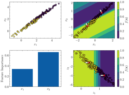
Figure 1: The GRBF-NN behavior is graphically represented in four subfigures: the upper left figure shows the classification problem with purple and yellow dots representing the two classes. The upper right figure shows the fitted GRBF-NN in the input space, while the lower right figure shows the fitted GRBF-NN model in the active subspace. Contour levels show estimated class probabilities. The red dotted points represent the GRBF-NN centers. The white arrow highlights the direction of the dominant eigenvector $\mathbf{v}_{1}$. Finally, the lower left subfigure shows the feature importance estimated from the GRBF-NN.

Another example of a classification problem is shown in Fig. 2. In this case, we have two noisy interleaving half circles with $N=100$ and $D=2$, as seen in Fig. 2 (upper left figure). To achieve a stronger discriminative power from the model, we choose $M=16$ centers. In contrast to the previous example, not all of the model $f$ variability is concentrated along the direction identified by the eigenvector $\mathbf{v}_{1}$ related to the dominant eigenvalue $\gamma_{1}$. In this case, the fraction $\frac{\gamma_{1}}{\sum_{k}^{K}\gamma_{k}}$ is approximately 0.8, meaning that the resulting feature importance in Eq. 21 includes the contribution of the eigenvector $\mathbf{v}_{2}$. This is highlighted in the barplot in Fig 2 (lower left figure), where we decomposed the feature importance showing the contribution of each term in Eq. 21. Since $\mathbf{v}_{2}$ is orthogonal to $\mathbf{v}_{1}$, it gives more importance to the feature $x_{2}$ because $\mathbf{v}_{1}$ is quasi-parallel to the input $x_{1}$.

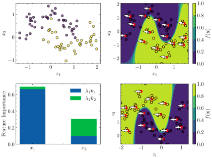
Figure 2: The GRBF-NN behavior is graphically represented in four subfigures: the upper left figure shows the classification problem with purple and yellow dots representing the two classes. The upper right figure shows the fitted GRBF-NN in the input space, while the lower right figure shows the fitted GRBF-NN model in the active subspace. Contour levels show estimated class probabilities. The red dotted points represent the GRBF-NN centers. The white arrow highlights the direction of the dominant eigenvector $\mathbf{v}_{1}$. Finally, the lower left subfigure shows the feature importance estimated from the GRBF-NN.

We present an example of regression, where the function to be approximated is $y=\sin(ax_{1}+bx_{2})$, with $a$ and $b$ being real scalars. Fig. 3 shows the case where $a$ and $b$ are equal to 0.5, and the true function is depicted in Fig. 3 (upper left figure). We then use our proposed model to obtain an approximation, as shown in Fig. 3 (upper right figure) along the direction given by the eigenvector $\mathbf{v}_{1}$, with the centers represented by dotted red points. Furthermore, we perform a supervised dimensionality reduction from the original two-dimensional space to the one-dimensional subspace defined by the first eigenvector $\mathbf{v}_{1}$. This subspace captures the ’active’ part of the function where most of the variation is realized, as illustrated in Fig. 3 (lower right figure). Finally, we estimate the feature importance using Eq. 21 and find that $x_{1}$ and $x_{2}$ contribute equally, as expected. This result is depicted in Fig. 3 (lower left figure).

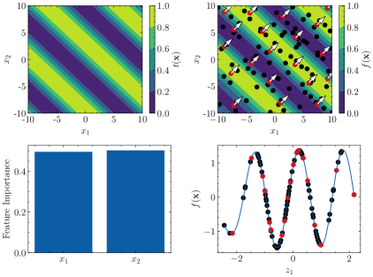
Figure 3: The GRBF-NN behavior is depicted in four subfigures: the upper left shows the regression problem $y=t(\mathbf{x})=\sin(0.5x_{1}+0.5x_{2})$, while the upper right displays the fitted GRBF-NN in the input space. The dominant eigenvector $\mathbf{v}_{1}$ is indicated by a white arrow, and the GRBF-NN centers are shown as red dotted points. The lower right shows the fitted GRBF-NN model projected in the one-dimensional active subspace. The function values at the input data and at the centers are represented by black and red dotted points, respectively. Finally, the lower left subfigure displays the feature importance estimated from the GRBF-NN. Function values are normalized.

In this final example, we altered the values of the scalars $a$ and $b$ to 0.1 and 0.9, respectively. This modification resulted in a change in the feature importance estimated by our model, as depicted in Fig. 4.

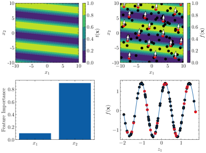
Figure 4: The GRBF-NN behavior is depicted in four subfigures: the upper left shows the regression problem $y=t(\mathbf{x})=\sin(0.1x_{1}+0.9x_{2})$, while the upper right displays the fitted GRBF-NN in the input space. The dominant eigenvector $\mathbf{v}_{1}$ is indicated by a white arrow, and the GRBF-NN centers are shown as red dotted points. The lower right shows the fitted GRBF-NN model projected in the one-dimensional active subspace. The function values at the input data and at the centers are represented by black and red dotted points, respectively. Finally, the lower left subfigure displays the feature importance estimated from the GRBF-NN. Function values are normalized.

In summary, the GRBF-NN model beyond solving a classical regression/classification model provides the user with valuable information about the model behavior such as allowing visualization of the fitted model $f$ of the active subspace thereby recognizing the underlying factors of variation of the data, and in parallel allowing to discover which are the most important input features related to the prediction task.

4 Numerical Experiments

This section aims to provide a comprehensive evaluation of the proposed model by assessing its predictive performance and feature selection quality. We consider two variants of the GRBF-NN model, one with unsupervised center selection (GRBF-NN_k) as given in Eq. 11 and the other with supervised center selection (GRBF-NN_c) as given in Eq. 13. We compare the performance of these models with other popular models such as Multi-Layer Perceptron (MLP) and Support Vector Machines (SVMs) cortes1995support . As the GRBF-NN model incorporates feature selection, it can be classified as an embedding method. To provide a comprehensive benchmark, we also include other widely used embedding methods such as Random Forest (RF) friedman1991multivariate and Gradient Boosting (GB) friedman2001greedy , which have shown strong performance for tabular data. In addition, we include state-of-the-art embedding deep learning methods such as Deep Feature Selection (DFS) li2016deep and the method proposed in wojtas2020feature , referred to as FIDL (Feature Importance for Deep Learning) in this comparison for simplicity.

4.1 Datasets

To test the predictive performance of our model we consider 20 different real-world problems as summarized in Tab. 1. We have a total of 6 binary classifications, 4 multiclass, 1 time series, and 9 regression problems. In the following, we provide a description of each of them:

• Digits alimoglu1996methods : They created a digit database by collecting 250 samples from 44 writers. The samples written by 30 writers are used for training, cross-validation and writer-dependent testing, and the digits written by the other 14 are used for writer-independent testing. For the current experiment, we use the digits $3$ and $8$ for feature selection purposes so that $N=357$ and $D=64$.

• Iris fisher1936use : One of the most famous datasets in the pattern recognition literature, contains 3 classes of 50 instances each ($N=150,D=4$), where each class refers to a type of iris plant. One class is linearly separable from the other 2; the latter are not linearly separable from each other.

• Breast Cancer street1993nuclear : Features are computed from a digitized image of a fine needle aspirate (FNA) of a breast mass. They describe the characteristics of the cell nuclei present in the image. In this dataset, $N=569$, $D=30$, and two classes.

• Wine aeberhard1994comparative : The data is the results of a chemical analysis of wines grown in the same region in Italy by three different cultivators. There are thirteen different measurements taken for different constituents found in the three types of wine. In this dataset, $N=173$, $D=13$, and three classes.

• Australian Dua:2019 : This is the famous Australian Credit Approval dataset, originating from the StatLog project. It concerns credit card applications. All attribute names and values have been changed to meaningless symbols to protect the confidentiality of the data. In this dataset, $N=600$, $D=15$, and two classes.

• Credit-g Dua:2019 : This dataset classifies people described by a set of attributes as good or bad credit risks, there are $D=20$ features, $N=1000$ data points, and two classes in this dataset.

• Glass evett:1987:rifs : The Glass identification database. The study of the classification of types of glass was motivated by criminological investigation. There are $D=9$ features, $N=214$ data points, and two classes in this dataset.

• Blood YEH20095866 : Data taken from the Blood Transfusion Service Center in Hsin-Chu City in Taiwan. The center passes its blood transfusion service bus to one university in Hsin-Chu City to gather blood donated about every three months. The target attribute is a binary variable representing whether he/she donated blood in March 2007. There are $D=4$ features, $N=748$ data points, and two classes in this dataset.

• Heart Disease Dua:2019 : This database contains 76 attributes, but all published experiments refer to using a subset of $D=14$ of them and $N=270$. The goal is to predict the presence of heart disease in the patient.

• Vowel deterding1989speaker : Speaker-independent recognition of the eleven steady state vowels of British English using a specified training set of lpc derived log area ratios. There are $D=12$ features, $N=990$ data points, and eleven classes in this dataset.

• Dehli Weather DWdataset : The Delhi weather dataset was transformed from a time series problem into a supervised learning problem by using past time steps as input variables and the subsequent time step as the output variable, representing the humidity. In this dataset $N=1461$ and $D=7$.

• Boston pace1997sparse : This dataset contains information collected by the U.S Census Service concerning housing in the area of Boston Mass and has been used extensively throughout the literature to benchmark algorithms for regression. In this dataset $N=506$ and $D=14$.

• Diabetes smith1988using : Ten baseline variables, age, sex, body mass index, average blood pressure, and six blood serum measurements were obtained for each of $N=442$ diabetes patients, as well as the response of interest, a quantitative measure of disease progression one year after baseline.

• Prostatic Cancer stamey1989prostate : The study examined the correlation between the level of prostate-specific antigen (PSA) and a number of clinical measures, in $N=97$ men who were about to receive a radical prostatectomy. The goal is to predict the log of PSA (lpsa) from a number of measurements of $D=4$ features.

• Liver MCDERMOTT201641 : It is a regression problem where he first 5 variables are all blood tests that are thought to be sensitive to liver disorders that might arise from excessive alcohol consumption. Each line in the dataset constitutes the record of a single male individual. There are $D=5$ features, $N=345$ data points.

• Plasma nierenberg1989determinants : A cross-sectional study has been designed to investigate the relationship between personal characteristics and dietary factors, and plasma concentrations of retinol, beta-carotene, and other carotenoids. Study subjects ($N=315$) were patients who had an elective surgical procedure during a three-year period to biopsy or remove a lesion of the lung, colon, breast, skin, ovary, or uterus that was found to be non-cancerous.

• Cloud Dua:2019 : The data sets we propose to analyze are constituted of $N=1024$ vectors, each vector includes $D=10$ parameters. Each image is divided into super-pixels 16*16 and in each super-pixel, we compute a set of parameters for the visible (mean, max, min, mean distribution, contrast, entropy, second angular momentum) and IR (mean, max, min).

• DTMB-5415 dagostino2020design : The DTMB-5415 datasets come from a real-world naval hydrodynamics problem. The $21$ input variables represent the design variables responsible for the shape modification of the hull while the output variable represents the corresponding total resistance coefficient of the simulated hull through a potential flow simulator. We propose two versions of the same problem: DTMB-$5415^{1}$ where all the $21$ design variables are related to the output variable and DTMB-$5415^{2}$ where $5$ of the $21$ design variables are not related to the output so that in this manner we can evaluate the models also from a feature selection perspective.

• Body Fat penrose1985generalized : Estimates of the percentage of body fat are determined by underwater weighing and various body circumference measurements for $N=252$ men and $D=14$ different input features.

Table 1: Datasets considered in the benchmark.

Name	$N$	$D$	Task	Reference
Digits	357	64	Binary classification	alimoglu1996methods
Iris	150	4	Multiclass classification	fisher1936use
Breast Cancer	569	30	Binary classification	street1993nuclear
Wine	173	13	Multiclass classification	aeberhard1994comparative
Australian	600	15	Binary classification	Dua:2019
Credit-g	1000	20	Binary classification	Dua:2019
Glass	214	9	Multiclass classification	evett:1987:rifs
Blood	748	4	Binary classification	YEH20095866
Heart Disease	270	13	Binary classification	Dua:2019
Vowel	990	12	Multiclass classification	deterding1989speaker
Delhi Weather	1461	7	Time series	DWdataset
Boston Housing	506	14	Regression	pace1997sparse
Diabetes	214	9	Regression	smith1988using
Prostatic Cancer	97	4	Regression	stamey1989prostate
Liver	345	5	Regression	MCDERMOTT201641
Plasma	315	16	Regression	nierenberg1989determinants
Cloud	108	5	Regression	Dua:2019
DTMB-$5415^{1}$	42	21	Regression	dagostino2020design
DTMB-$5415^{2}$	42	21	Regression	dagostino2020design
Body Fat	252	14	Regression	penrose1985generalized

Furthermore, we use synthetic datasets to provide a deeper comparison of the feature importance and feature selection results obtained by the methods since the ground truth of the feature importance related to the learning task is known. This allows for the evaluation of the quality of the feature selection and ranking provided by the methods, as the true feature importance can be compared to the estimates obtained by the models. The synthetic datasets considered are the following:

• Binary classification hastie2009elements (P1): given $y=-1$, the ten input features are generated with $(x_{1},\dots,x_{10})\sim\mathcal{N}(0,\mathbf{I}_{10})$. Given $y=1$, $x_{1}$ through $x_{4}$ are standard normal conditioned on $9\leq\sum_{j=1}^{4}x_{j}^{2}\leq 16$, and $(x_{5},\dots,x_{10})\sim\mathcal{N}(0,\mathbf{I}_{6})$.
  The first four features are relevant for P1.

• $3$-dimensional XOR as 4-way classification chen2017kernel (P2): Consider the 8 corners of the 3-dimensional hypercube $(v_{1},v_{2},v_{3})\in{-1,1}^{3}$, and group them by the tuples $(v_{1}v_{3},v_{2}v_{3})$, leaving 4 sets of vectors paired with their negations ${v^{(i)},-v^{(i)}}$. Given a class $i$, a point is generated from the mixture distribution $(1/2)\mathcal{N}(v^{(i)},0.5\mathbf{I}_{3})+(1/2)\mathcal{N}(-v^{(i)},0.5\mathbf{I}_{3})$. Each example additionally has 7 standard normal noise features for a total of $D=10$ dimensions.
  The first three features are relevant for P2.

• Nonlinear regression friedman1991multivariate (P3): The $10$-dimensional inputs $x$ are independent features uniformly distributed on the interval $[0,1]$. The output $y$ is created according to the formula $y=10\sin(\pi x_{1}x_{2})+20(x_{3}-0.5)^{2}+10x_{4}+5x_{5}+\epsilon$ with $\epsilon\sim\mathcal{N}(0,1)$.
  The first five features are relevant for P3.

In all those three cases we varied the number of data points with $N\in\{100,500,1000\}$.

4.2 Numerical Set-up

In this section, we present the numerical details of our experiment. We evaluate the performance of the GRBF-NN model for feature selection with unsupervised (GRBF-NN_k) and supervised (GRBF-NN_c) center selection, as defined in Eq.11 and Eq. 13, respectively. To compute the centers for GRBF-NN_k, we use the popular $k$-means clustering algorithm. Both GRBF-NN_$c$ and GRBF-NN_$k$ were optimized using Adam kingma2014adam for a maximum of 10000 epochs. We implemented the GRBF-NN in Pytorch NEURIPS2019_9015 .

We perform a grid search to approximately find the best set of hyperparameters of all the models considered in these numerical experiments.
For the GRBF-NN the grid search is composed as follows:

• Number of centers: For regression problems, the number of centers $M$ can take the following values $M\in\{8,32,128\}$, where for classification $M\in\{2,4,8,16,32\}$.

• Regularizers: $(\lambda_{\mathbf{w}}$, $\lambda_{\mathbf{u}})\in\{0,10^{-3},10^{-2},10^{-1},1,10^{1},10^{2},10^{3}\}$.

• Adam learning rate: $\alpha\in\{10^{-3},10^{-2}\}$.

For the SVM model, we used a Gaussian kernel, and the grid search is composed as follows:

• Gaussian kernel width: $\sigma^{2}\in\{0,10^{-3},10^{-2},10^{-1},1,10^{1},10^{2},10^{3}\}$.

• Regularizer: $C\in\{0,10^{-3},10^{-2},10^{-1},1,10^{1},10^{2},10^{3}\}$.

For the RF model, the grid search is composed as follows:

• Depth of the tree: $d_{t}\in\{2,4,8,16,32,64,128\}$.

• Minimum number of samples required to be a leaf node: $s_{t}\in\{1,5,10,20\}$.

• Number of decision trees: $n_{t}\in\{10,20,50,100,200,400,800\}$.

For the GB model, the grid search is composed as follows:

• Learning rate: $l_{b}\in\{10^{-3},10^{-2},10^{-1},1\}$.

• Number of boosting stages: $n_{b}\in\{10,20,50,100,200,400,800\}$.

• Maximum depth of the individual regression estimators: $d_{b}\in\{2,4,8,16,32,64,128\}$.

For the MLP the grid search is composed as follows:

• Regularizer ($L2$-norm): $\lambda\in\{0,10^{-3},10^{-2},10^{-1},1,10^{1},10^{2},10^{3}\}$

• Network architecture: A two-hidden-layer architecture with the following combinations of the number of neurons in the two layers is considered $\{(D,\lceil D/2\rceil)),(2D,D),(2D,\lceil D/2\rceil)\}$ with rectifiers activation functions fukushima1975cognitron .

• Adam learning rate: $\alpha\in\{10^{-3},10^{-2}\}$.

For the DFS we use the same grid search hyperparameters as in the MLP case. This is because the DFS is the same as an MLP but with an additional sparse one-to-one layer added between the input and the first hidden layer, where each input feature is weighted. We use the implementation available on the following link .
For the FIDL, we use the author’s implementation of the algorithm available at the following link and the following grid search hyperparameters:

• Network architecture: A two-hidden-layer architecture with the following combinations of the number of neurons in the two layers is considered $\{(D,\lceil D/2\rceil)),(2D,D),(2D,\lceil D/2\rceil)\}$.

• Number of important features: $s=\lceil D/2\rceil$.

Always referring to FIDL, for datasets that are used also in their paper, we use the optimal set of hyperparameters found by them. In this method, the user has to choose in advance, and before training the model, the number of important features $s$ that the problem might have. We fix this parameter to $s=\lceil D/2\rceil$ as used in their paper for some datasets. We fix all the other hyperparameters to their default values provided by the authors.

We perform a 5-fold cross-validation to identify the best set of hyperparameters for the models. Once the best set of hyperparameters is determined, we conduct another 5-fold cross-validation using 20 different seeds to obtain statistically significant results. For the Dehli Weather dataset we used a 5-fold cross-validation on a rolling basis because it is a time series problem. For the FIDL model, we were able to run the cross-validation procedure with respect to its best set of hyperparameters varying only time the random seed due to the severe time and memory complexity of the model. For the regression problems we use a root mean squared error (RMSE) while for the classification problems, we use the accuracy as a metric to evaluate the models. For the SVM, MLP, RF, and GB we used the Python package scikit-learn .

4.3 Numerical Results

4.3.1 Evaluation of the Predictive Performance

Tab. 2 presents a summary of our numerical results, showing the mean from the cross-validation procedure for each model. Notably, the GRBF-NN demonstrates strong competitiveness compared to the other models. In twelve out of twenty datasets, the GRBF-NN shows a better performance. The SVM and RF are the best models on three different datasets, MLP and the FIDL in two datasets, the GB in one, and the DFS in none of them. Regarding the comparison between the GRBF-NN_$c$ and GRBF-NN_$k$, the numerical results indicate that there is not a clear winner and that both strategies for selecting centers are equally competitive and the user might consider trying both of them. In some datasets, the optimizer used for the training process of FIDL did not seem to converge to a decent stationary point and the resulting performance in those datasets is not reported.

In the classification tasks, the GRBF-NN achieves the best accuracy on the Digits, Iris, Breast Cancer, and Wine datasets. Furthermore, in all those cases the best results are obtained using an unsupervised selection of the centers namely the GRBF-NN_$k$ model. The SVM shows the best performance on the Credit-g and the Vowel datasets while the RF model achieves the highest accuracy on the Blood and the Australian datasets whereas in the latter the MLP achieves a comparable performance. The GB and FIDL achieve the best performance on the Glass and the Heart Disease datasets. The DFS model seems not to outperform the other models in any of the classification tasks.

In regression tasks, the GRBF-NN demonstrates even stronger competitiveness, with lower RMSE than other models in eight out of ten datasets. Differently from the classification cases, here the supervised selection of the centers, namely the GRBF-NN_$c$ seems to be more effective than GRBF-NN_$k$. In this case, the SVM, RF, and FIDL are the best performing in only one case each which are the Prostatic Cancer, Diabetes, and the Cloud datasets respectively. The GB and the DFS do not outperform in any of the regression tasks considered.

Table 2: Numerical results summary: first ten datasets are for binary and multiclass classification, showing average accuracy achieved via cross-validation. The last ten are for regression and time series, showing average RMSE via cross-validation. Bold numbers indicate the best performing method on the test datasets.

	GRBF-NN$k$		GRBF-NN$c$		SVM		RF		GB		MLP		DFS		FIDL
	Training	Test	Training	Test	Training	Test	Training	Test	Training	Test	Training	Test	Training	Test	Training	Test
Digits	1.000	$\mathbf{0.994}$,	0.995	0.989	1.000	0.992	1.000	0.990	1.000	0.983	1.000	0.993	1.000	0.990	0.999	0.972
Iris	0.982	$\mathbf{0.971}$	0.943	0.941	0.974	0.958	0.989	0.949	0.989	0.951	0.984	0.958	0.985	0.959	0.962	0.967
Breast Cancer	0.987	$\mathbf{0.978}$	0.988	0.976	0.988	0.977	1.000	0.971	0.990	0.956	1.000	0.965	0.985	0.976	0.992	0.974
Wine	0.996	$\mathbf{0.985}$	0.991	0.979	0.992	0.983	1.000	0.971	1.000	0.980	1.000	0.976	1.000	0.984	1.000	0.961
Australian	0.911	0.861	0.853	0.847	0.884	0.858	0.924	$\mathbf{0.868}$	0.998	0.865	1.000	$\mathbf{0.868}$	0.818	0.812	0.883	0.851
Credit-g	0.787	0.760	0.812	0.758	0.841	$\mathbf{0.765}$	0.874	0.744	1.000	0.760	0.905	0.764	0.778	0.757	0.793	0.747
Glass	0.912	0.657	0.969	0.686	0.857	0.685	0.978	0.714	1.000	$\mathbf{0.780}$	1.000	0.748	0.947	0.710	0.699	0.630
Blood	0.791	0.781	0.794	0.782	0.829	0.784	0.801	$\mathbf{0.792}$	0.818	0.790	0.855	0.771	0.789	0.777	0.762	0.762
Heart Disease	0.849	0.824	0.846	0.814	0.943	0.802	0.872	0.842	0.916	0.834	0.951	0.816	0.891	0.826	0.878	$\mathbf{0.844}$
Vowel	0.995	0.959	0.998	0.969	0.999	$\mathbf{0.992}$	1.000	0.968	1.000	0.967	1.000	0.907	0.995	0.953	-	-
Delhi Weather	0.115	0.111	0.098	$\mathbf{0.107}$	0.109	0.108	0.071	0.190	0.062	0.162	0.106	0.110	0.541	0.371	-	-
Boston Housing	0.224	$\mathbf{0.344}$	0.217	0.361	0.181	0.361	0.211	0.359	0.135	0.364	0.042	$\mathbf{0.344}$	0.280	0.388	-	-
Diabetes	0.703	0.718	0.669	$\mathbf{0.706}$	0.680	0.711	0.655	$\mathbf{0.706}$	0.662	0.745	0.590	0.737	0.661	0.711	-	-
Prostatic Cancer	0.581	0.646	0.581	0.646	0.570	$\mathbf{0.625}$	0.595	0.662	0.610	0.715	0.349	0.718	0.460	0.697	0.408	0.644
Liver	0.834	$\mathbf{0.895}$	0.838	0.902	0.825	0.913	0.857	0.911	0.770	0.923	0.731	0.931	0.846	0.934	-	-
Plasma	0.958	0.991	0.941	$\mathbf{0.982}$	0.937	0.987	0.890	0.989	0.984	1.001	1.000	1.002	0.917	1.070	-	-
Cloud	0.340	0.451	0.323	0.385	0.344	0.373	0.378	0.417	0.418	0.521	0.191	0.433	0.615	0.613	0.138	$\mathbf{0.206}$
DTMB-$5415^{(1)}$	0.513	$\mathbf{0.752}$	0.103	0.783	0.096	0.886	0.009	0.816	0.413	1.014	0.034	0.919	0.777	0.898	0.899	0.932
DTMB-$5415^{(2)}$	0.031	0.112	0.020	$\mathbf{0.071}$	0.088	0.226	0.052	0.238	0.342	0.902	0.000	0.808	0.048	0.300	0.073	0.077
Body Fat	0.090	0.132	0.086	$\mathbf{0.127}$	0.153	0.148	0.074	0.131	0.070	0.170	0.029	0.166	0.113	0.137	1.523	2.650

The strip plots shown in Fig. 5 and in Fig. 6 illustrate the data obtained from our experiment. Notably, the RF and GB exhibit signs of overfitting in some datasets as they perform exceptionally well on the training data in multiple datasets yet fail to maintain the same level of performance on the estimated test error/accuracy. This discrepancy is particularly noticeable in datasets such as Breast cancer, Credit-g, Australian, Diabetes, Prostatic Cancer, Liver, and Boston Housing where there is a significant disparity between the estimated training and test error/accuracy. We can notice also that the RBF-NN_$c$ occasionally exhibits high standard deviation in both training and test metrics. This is due to the presence of outliers, which could signify potential challenges that arose during the training process, such as the optimizer converging to a suboptimal stationary point of the error function described in Eq. 13. This pattern was observed in the Digits, Iris, Wine, and Australian datasets.

Digits	Iris
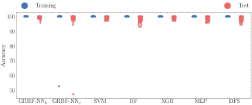
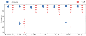
Breast Cancer	Wine
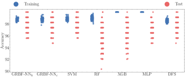
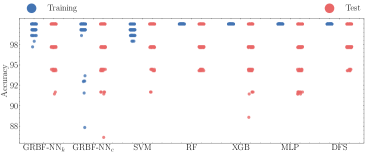
Australian	Credit-g
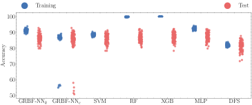
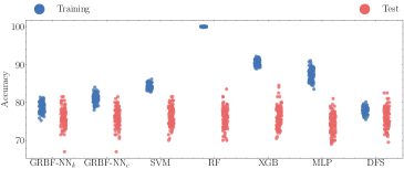
Glass	Blood
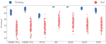
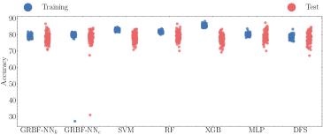
Heart Disease	Vowel

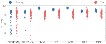
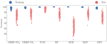
Figure 5: Strip plots of the numerical results obtained in Tab. 2 regarding the first ten datasets (classification). In blue and red are the data for training and test sets respectively. The accuracy on the y-axis.

Delhi Weather	Boston Housing
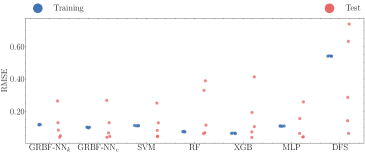
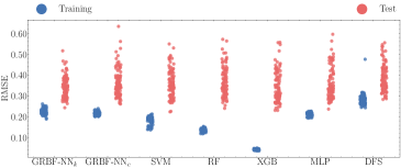
Diabetes	Prostatic cancer
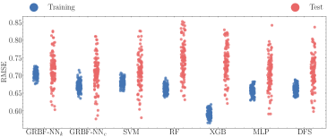
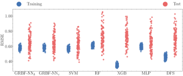
Liver	Plasma
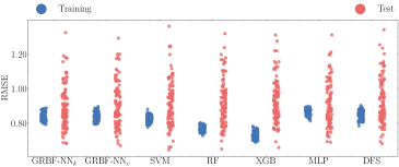
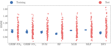
Cloud	DTMB-$5415^{(1)}$
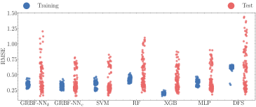
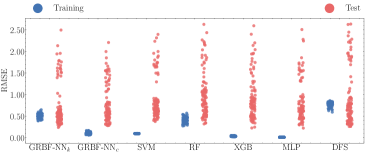
DTMB-$5415^{(2)}$	Body Fat

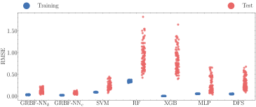
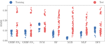
Figure 6: Strip plots of the numerical results obtained in Tab. 2 regarding the last ten datasets (regression). In blue and red are the data for training and test sets respectively. The RMSE on the y-axis.

We aim to provide further insights into the behavior of the GRBF-NN model by examining the relationship between its two regularizers, $\lambda_{\mathbf{w}}$ and $\lambda_{\mathbf{u}}$, through graphical analysis in Fig. 9. For every dataset, we show the results of the hyperparameter search procedure for training and test datasets. We only show the best model between GRBF-NN_$k$ and the GRBF-NN_$c$ for each dataset.

For the regression problems, dark colors indicate lower error while for classification problems lighter color indicates higher accuracy. The red frame indicates the best set of regularizers. Interestingly, in many datasets, we observe that the regularizer of the precision matrix $\lambda_{\mathbf{u}}$ impacts the performance of the GRBF-NN more than the regularizer of the weights $\lambda_{\mathbf{w}}$. This phenomenon occurs in the Digits, Breast Cancer (see Fig. 7(b)), Credit-g, Glass, Diabetes, Prostatic Cancer (see Fig. 8(b)), Cloud, DTMB-$5415^{(2)}$ and in the Body Fat dataset. In these cases, we obtain the best combination of regularizers on the test data when $\lambda_{\mathbf{w}}$ is set to 0. This suggests that the regularization term $\lambda_{\mathbf{w}}$ has minimal influence on the learning task on those datasets.

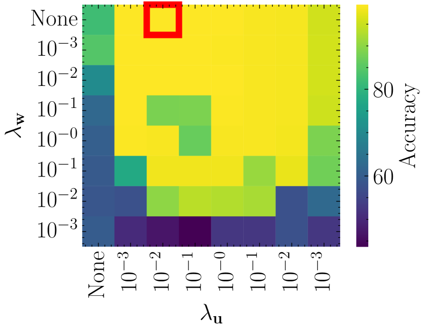
(a) Breast Cancer dataset training accuracies.

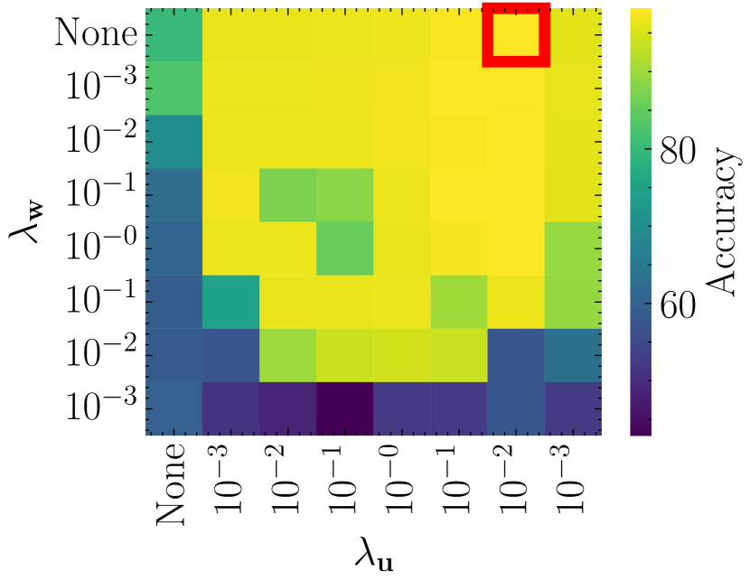
(b) Breast Cancer dataset test accuracies.

Figure 7: Graphical interpretation of the sensitivity analysis with respect to the two regularizers $\lambda_{\mathbf{w}}$ and $\lambda_{\mathbf{u}}$ on the Breast Cancer dataset (binary classification). The red frame highlights the best combination of hyperparameters. Lighter color indicates higher accuracy.

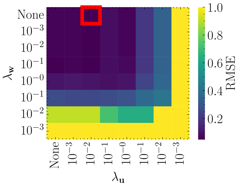
(a) Prostatic Cancer dataset training error.

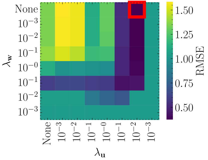
(b) Prostatic Cancer dataset test error.

Figure 8: Graphical interpretation of the sensitivity analysis with respect to the two regularizers $\lambda_{\mathbf{w}}$ and $\lambda_{\mathbf{u}}$ on the Prostatic Cancer dataset (regression). The red frame highlights the best combination of hyperparameters. Darker color indicates lower error.

This can indicate that promoting the ’flatness’ of the Gaussian basis function through penalizing the entries of the precision matrix $\mathbf{M}$ may have a more pronounced regularization and generalization impact on the model than merely penalizing the amplitudes via $\lambda_{\mathbf{w}}$. Therefore, in situations where conducting a large hyperparameter search is not feasible due to computational constraints, it might be beneficial to prioritize the hyperparameter search solely on $\lambda_{\mathbf{u}}$.

	Digits	Iris	Breast Cancer	Wine
Training
Test
	Australian	Credit-g	Glass	Blood
Training
Test
	Heart Disease	Vowel	Delhi Weather	Boston Housing
Training
Test
	Diabetes	Prostatic Cancer	Liver	Plasma
Training
Test
	Cloud	DTMB-$5415^{(1)}$	DTMB-$5415^{(2)}$	Body Fat
Training
Test

Figure 9: GRBF-NN’s behavior with respect to regularization: dark color for lower RMSE (regression) and lighter for higher accuracy (classification). The red frame indicates the best regularization combination.

In section 3.1, we mentioned that valuable insights into the behavior of the GRBF-NN can be obtained by examining the eigenvalues and projecting the problem onto the active subspace defined by the eigenvectors of $\mathbf{M}$. This enables us to visualize the function the GRBF-NN is attempting to model (for example, in $2D$) as demonstrated in Fig. 12, offering users an additional approach to comprehending the representation learned by our model.

The first row of the plots shows the reduced representation of the original problem in the active subspace or latent space $\mathbb{Z}\subset\mathbb{R}^{K}$ once the training of the GRBF-NN has been completed. In particular, we project the dataset $\mathbf{X}$, along the first two eigenvectors relative to the largest eigenvalues of the matrix $\mathbf{M}$, for visualization in $2D$. We calculate the function value of the GRBF-NN simply by performing the inverse map of the latent variables $\mathbf{z}$ in the input space.

The second row of figures shows the fraction $\frac{\gamma_{1}}{\sum_{k}^{K}\gamma_{k}}$ sorted in descending order illustrating the eigenvalues decay. It is worth recalling that the eigenvalue $\gamma_{k}$ of the matrix $\mathbf{M}$ represents the second derivative of the argument of the Gaussian basis function after rotating it in the latent space, along the corresponding principal axis $\mathbf{v}_{k}$. Therefore, very low magnitudes eigenvalues mean a lack of variability of our model in those principal directions, indicating that the true underlying factors of variation of the original problem may develop in a lower dimensional space.

For example, for the Digits, Iris, and Breast Cancer datasets, the embedding shows that the function $f$ provides a remarkable discriminative power where most of the variability is obtained in just one dimension namely along the latent variable $z_{1}$. This is confirmed by the relative eigenvalues decays, which show that the first eigenvalue $\gamma_{1}$ is the only one significantly different from zero. In general, for almost linearly separable classification problems is likely that the GRBF-NN detects a one-dimensional active subspace as is also the case for the Heart Disease dataset. In the case of the Wine dataset instead (see Fig. 10), our model identifies an active subspace of dimension $K=2$. This indicates that in order to achieve high accuracy in discriminating among classes, the function $f$ mainly varies in two dimensions. This is further supported by the fact that the first two eigenvalues account for almost the entire model variability.

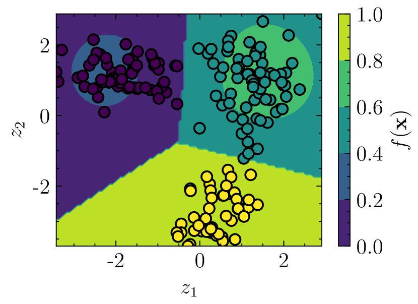
(a) Wine dataset active subspace.

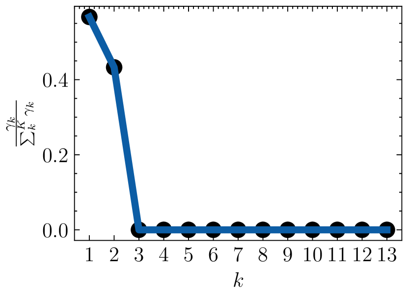
(b) Wine dataset eigenvalues decay.

Figure 10: Graphical interpretation of the active subspace in two dimensions (a) and corresponding eigenvalues decay (b) for the Wine dataset (multiclass classification). Function values are normalized between zero and one.

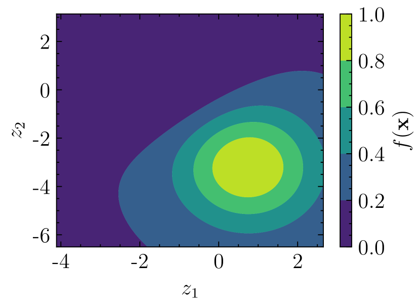
(a) Livers dataset active subspace.

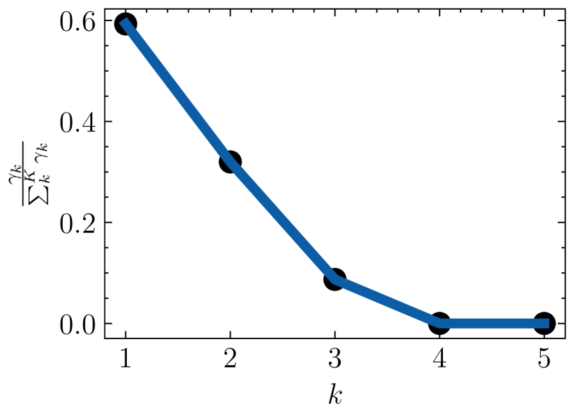
(b) Livers dataset eigenvalues decay.

Figure 11: Graphical interpretation of the active subspace in two dimensions (a) and corresponding eigenvalues decay (b) for the Liver dataset (regression). Function values are normalized between zero and one.

In the regression cases, we can, for example, observe that the GRBF-NN model identifies an active subspace of dimension $K=1$ in many datasets such as the Prostate Cancer, Plasma, Cloud, DTMB-$5415^{(1)}$ and the DTMB-$5415^{(2)}$ dataset. For the remaining regression problems, the form of $f$ is more complex, with its variation occurring in more than two dimensions as can be seen in the Liver dataset in Fig. 11.

	Digits	Iris	Breast cancer	Wine
Active subspace
Eigenvalues decay
	Australian	Credit-g	Glass	Blood
Active subspace
Eigenvalues decay
	Heart Disease	Vowel	Delhi Weather	Boston Housing
Active subspace
Eigenvalues decay
	Diabetes	Prostate cancer	Liver	Plasma
Active subspace
Eigenvalues decay
	Cloud	DTMB-$5415^{(1)}$	DTMB-$5415^{(2)}$	Body Fat
Active subspace
Eigenvalues decay

Figure 12: Graphical interpretation of the active subspace in two dimensions in the contour plots and corresponding eigenvalues decay. Function values are normalized.

4.3.2 Evaluation of the Feature Importance Ranking

In addition to analyzing the predictive performance and performing a supervised dimensionality reduction in the active subspace for visualization, we can also obtain information about the importance of input features $\mathbf{x}$. This provides additional insights into the model behavior and enables the user to perform feature selection. For the purpose of evaluating the significance of the feature importance ranking, we will only consider the embedding methods. This means that SVM and MLP will not be taken into account in this part of the benchmark since they do not provide information on the importance of each input feature.

Some of the datasets used to evaluate the predictive performance of the models can also be used to evaluate the quality of the feature importance ranking obtained once the model training has terminated such as the Digits and DTMB-$5415^{(2)}$ datasets. We train all the models using their best set of hyperparameters from the cross-validation procedure performed precedently with respect to the whole dataset.

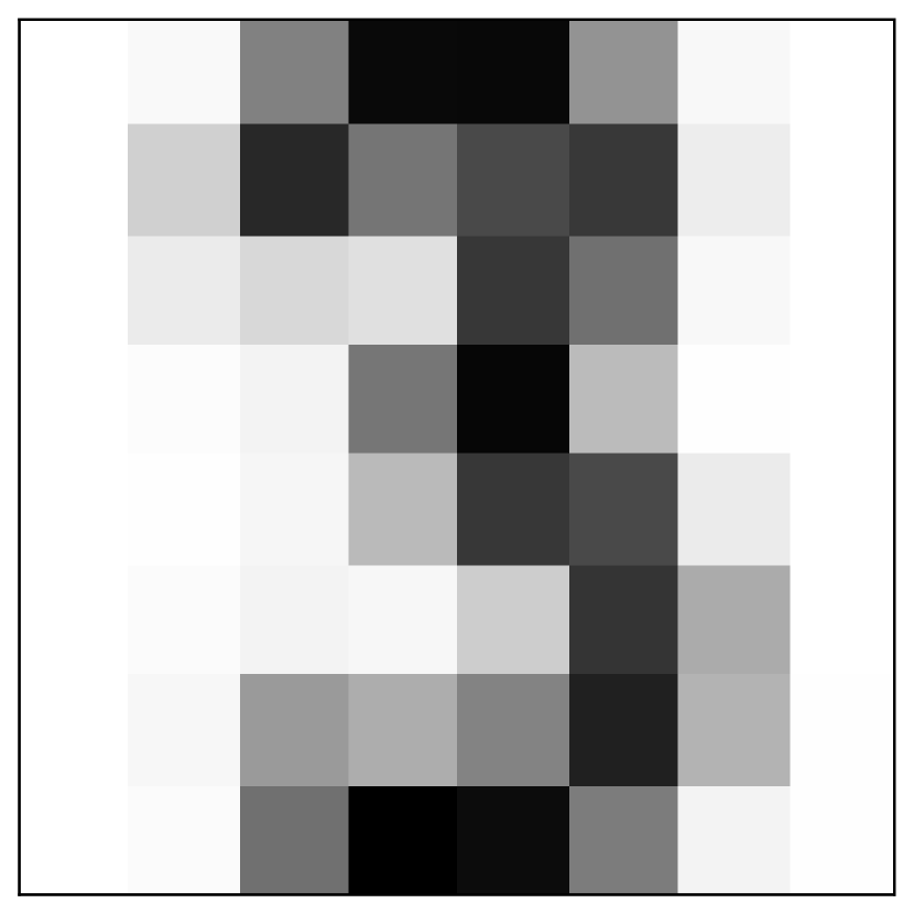
(a) Mean of the class ’3’.

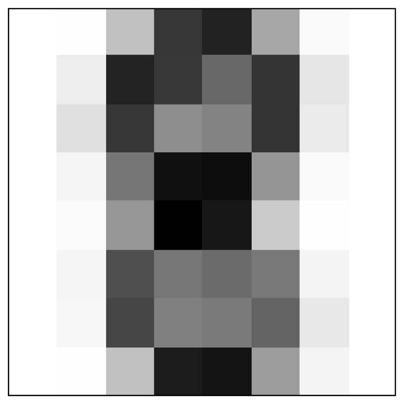
(b) Mean of the class ’8’.

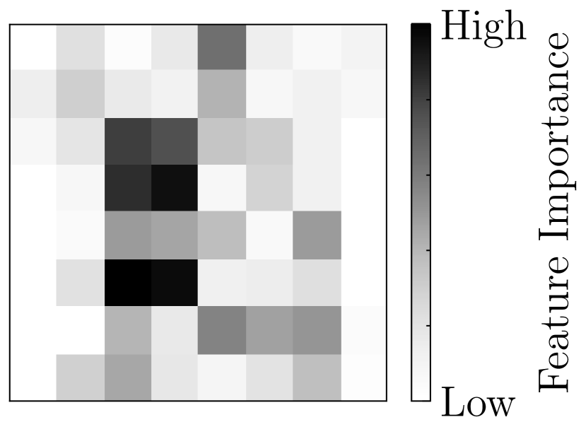
(c) GRBF-NN.

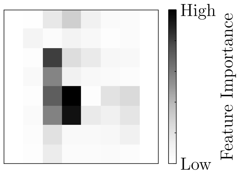
(d) RF.

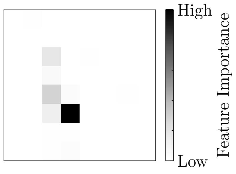
(e) GB.

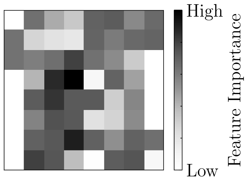
(f) DFS.

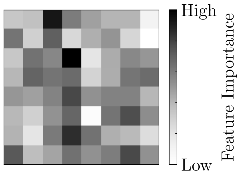
(g) FIDL.

Figure 13: Graphical interpretation of the feature importance for the Digits dataset for all the models considered in this experiment. The feature importance should highlight the pixels where (a) and (b) differ.

We can easily show the feature importance obtained from the Digits dataset, which is composed only of the digit ’8’ and ’3’. The mean of those two classes is visible in Fig. 13(a) and Fig. 13(b), where each feature corresponds to a particular pixel intensity of greyscale value. This suggests that is easy to interpret the feature importance identified from the models because the important features should highlight where the digits ’8’ and ’3’ differ the most. In Fig. 13 we can verify the feature importance detected from the models. The GRBF-NN employs an unsupervised center selection method for this dataset, as evidenced by the superior performance in Tab. 2 compared to the model with supervised center selection. Meaningful feature importance is observable for the GRBF-NN, RF, and GB models. The GRBF-NN (Fig. 13(c)), similar to the RF (Fig. 13(d)) the feature importance enhances pixels where those two classes differ, while the GB (Fig. 13(e)) provides a sparser representation since the almost all the importance is concentrated in only one pixel. From Fig. 13(f) and Fig. 13(g) seems that the two methods for feature importance learning for deep learning fail to provide explainable feature importances.

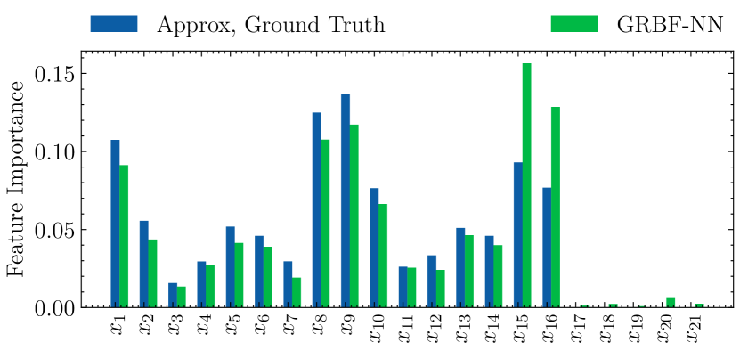
(a) GRBF-NN.

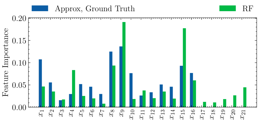
(b) RF.

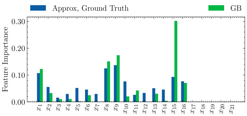
(c) GB.

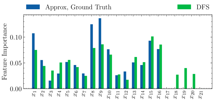
(d) DFS.

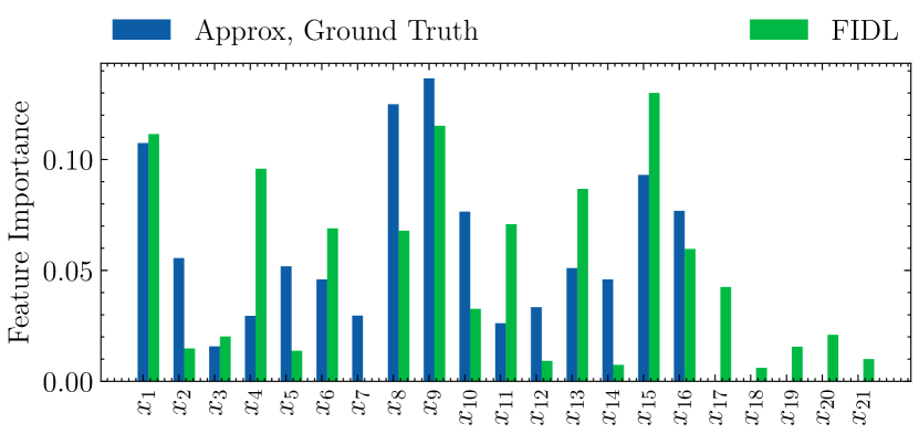
(e) FIDL.

Figure 14: Graphical interpretation of the feature importance for the DTMB-$5415^{(2)}$ dataset for all the models considered in this experiment. Blue bars represent the approximated ground truth feature importance, in green is the one estimated by the models.

We provide a similar validation analysis for the DTMB-$5415^{(2)}$ dataset. Based on the results presented in Tab. 2, the GRBF-NN model achieved better performance on this dataset using the supervised selection of the centers compared to the unsupervised selection of the centers. In these cases, we can estimate an approximate ground truth for the feature importance of the true function, by computing the gradients at specific input variables $\mathbf{x}$. To do this, we employ a finite difference process, evaluating gradients at 84 different points. The estimated ground truth is obtained by averaging the absolute values of the gradient vectors at these 84 points. In Fig. 14, we show the approximated ground truth in blue in each of the bar plots. It should be noted that the feature importance of the last five features is zero as these are not related to the true function, as explained in section 4.1. The feature importance obtained from the models shown in green should be able to detect this.

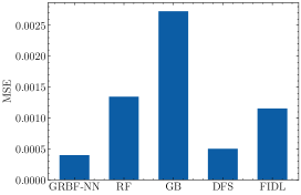
Figure 15: Bars represent the MSE ($y$-axis) between the approximated ground truth feature importance and the one estimated from the models ($x$-axis).

In this case, only the GRBF-NN and the GB are able to recognize that the last five features are not related to the true function $y$, while the RF (Fig. 14(b)), DFS (Fig. 14(d)) and FIDL (Fig. 14(e)) fail to identify that. To summarize the results, in Fig. 15 we show the bar plot regarding the mean squared error between the approximated ground truth feature importance and the one estimated from all the methods, showing that in this case, the GRBF-NN obtains the lowest error in detecting the underlying important variables of the regression task.

We test the same models on other synthetic datasets presented at the end of the section 4.1 designed specifically to evaluate feature selection and feature importance ranking models. In Tab. 3 we resume the numerical results obtained with the same cross-validation procedure as in the previous numerical experiments.

Table 3: Numerical results summary for the three synthetic problems. Problem 1 (P1) and Problem 2 (P2) are binary and multiclass classification tasks respectively and numbers represent the accuracy values. Problem 3 (P3) is a regression task and the numbers represent RMSE values. Bold numbers indicate the best performance on the test datasets.

		GRBF-NN$k$		GRBF-NN$c$		RF		GB		DFS		FIDL
	$N$	Training	Test	Training	Test	Training	Test	Training	Test	Training	Test	Training	Test
P1	100	0.980	0.609	1.000	0.652	0.992	0.672	1.000	$\mathbf{0.836}$	1.000	0.762	0.992	0.820
	500	0.958	0.898	0.981	0.892	1.000	0.882	1.000	$\mathbf{0.914}$	1.000	0.905	0.942	$\mathbf{0.914}$
	1000	0.962	$\mathbf{0.931}$	0.973	0.925	1.000	0.901	1.000	0.921	0.991	0.897	0.934	0.918
P2	100	0.235	0.310	0.250	0.249	1.000	0.290	1.000	0.273	0.973	0.338	0.762	$\mathbf{0.340}$
	500	0.710	0.428	0.706	$\mathbf{0.508}$	1.000	0.486	1.000	0.465	0.898	0.497	0.568	0.496
	1000	0.643	0.538	0.645	$\mathbf{0.551}$	0.871	0.546	1.000	0.492	0.633	0.537	0.497	0.455
P3	100	0.499	0.570	0.497	0.570	0.236	0.615	0.000	0.520	0.157	$\mathbf{0.447}$	-	-
	500	0.232	0.283	0.184	$\mathbf{0.255}$	0.163	0.440	0.105	0.324	0.190	0.289	-	-
	1000	0.258	0.284	0.198	$\mathbf{0.221}$	0.142	0.387	0.094	0.270	0.196	0.240	-	-

Problem P1 is a binary classification problem and the GB shows the best performance for $N=100$ and $N=500$ together with FIDL, while for $N=1000$ the GRBF-NN_$k$ obtained the higher accuracy. In Tab. 4, we have the feature importance related to problem P1. We discuss GRBF-NN_$c$ for $N=100$ while for $N=500$ and $N=1000$ we show GRBF-NN_$k$ and rename as GRBF-NN. For $N=100$, the GRBF-NN provides meaningless feature importance across the methods due also to the lack of predictive performance obtained in this case, while the GB and FIDL are the only models to recognize that the only first four features are related to the output $y$. For $N=500$ and $N=1000$, the feature importance from the GRBF-NN improves substantially together with its predictive performance. The DFS even if provides competitive accuracy compared with other methods has some difficulty in highlighting the importance of the first four features from the remaining ones especially for $N=500$. As further support and analysis, we can evaluate the eigenvalues decay that can help us to detect if the degrees of freedom of the variation of $f$ match approximately the correct number of the underlying factors of variation of the data. In Fig. 16, we have the eigenvalues decay for problem P1 for the values of $N$ considered. It is possible to notice that for $N=1000$ and $N=500$ the GRBF-NN varies mainly along four components which are also the number of the independent important features for P1, while for $N=100$, there is not a clear identification of those factors within the latent space/active subspace due to the low predictive performance of the model.

Table 4: Summary of the models feature importance obtained on problem P1. Note that the first four features are relevant in P1.

Model	GRBF-NN	RF	GB	DFS	FIDL
P1 ($N=100$)
P1 ($N=500$)
P1 ($N=1000$)

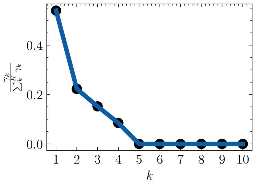
(a) $N=100$.

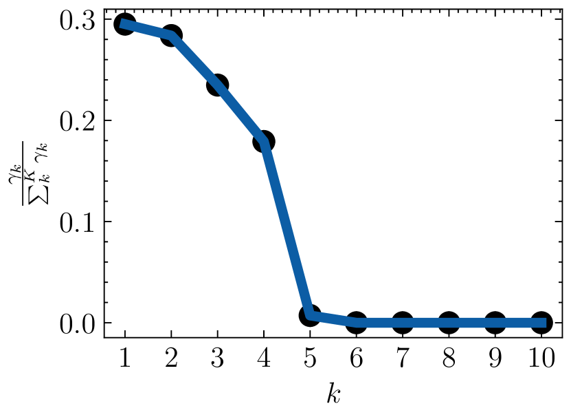
(b) $N=500$.

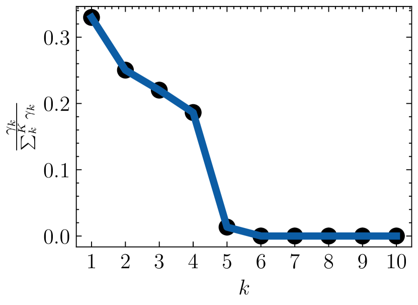
(c) $N=1000$.

Figure 16: Eigenvalues decay for problem P1.

Problem P2 is a difficult multiclass classification problem and FIDL shows the best performance for $N=100$ while for $N=500$ and $N=1000$ the GRBF-NN_$c$ obtains the highest accuracy. In Tab. 5, we have the feature importance related to problem P2. We discuss GRBF-NN_$k$ for $N=100$ while for $N=500$ and $N=1000$ we show GRBF-NN_$c$ and both renamed as GRBF-NN. Similarly as in the previous case for $N=100$, the GRBF-NN and RF have some difficulty to detect that the first three features are the most important while the FIDL provides the best feature ranking. Similar to problem P1, the feature importance from the GRBF-NN improves significantly for $N=500$ and $N=1000$ along with its predictive performance. The GRBF-NN and FIDL provide the most meaningful feature importance ranking in these cases, while the other methods fail to provide a clear separation between important and non-important variables. In Fig. 17, we have the eigenvalues decay for problem P2 for the values of $N$ considered. For $N=1000$, the GRBF-NN varies mainly along three components which are also the number of the independent important features for P2, this behavior is less visible but still present for $N=100$ and $N=500$.

Table 5: Summary of the models feature importance obtained on problem P2. Note that the first three features are relevant in P2.

Model	GRBF-NN	RF	GB	DFS	FIDL
P2 ($N=100$)
P2 ($N=500$)
P2 ($N=1000$)

(a) $N=100$.

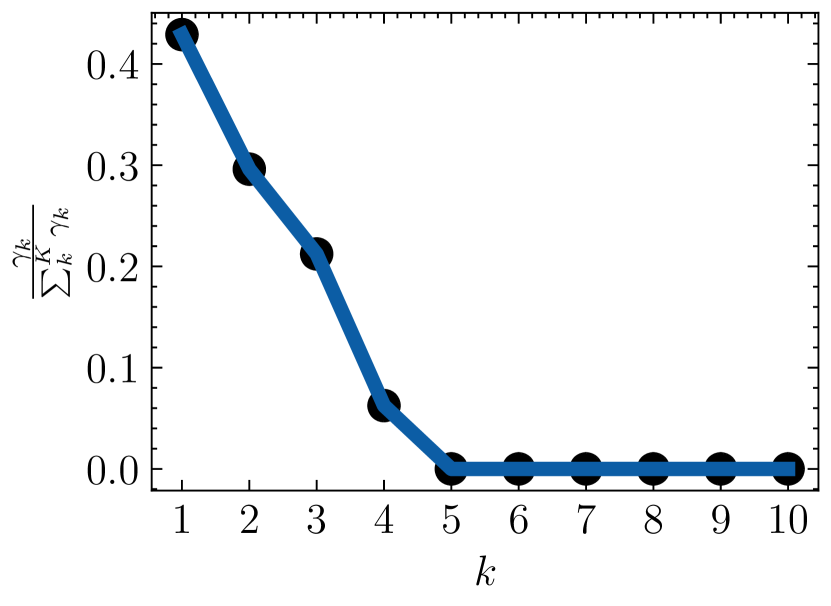
(b) $N=500$.

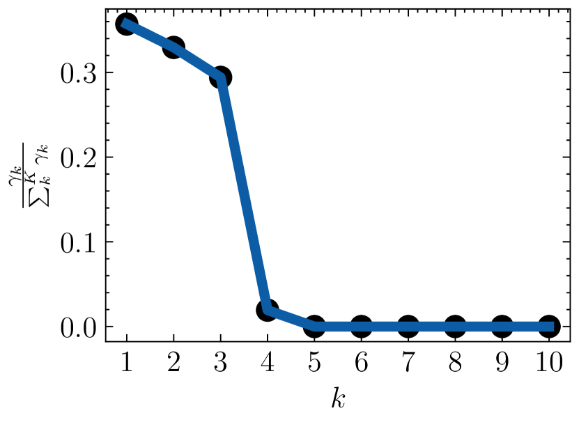
(c) $N=1000$.

Figure 17: Eigenvalues decay for problem P2.

Problem P3 is a nonlinear regression problem with the DFS showing the best performance for $N=100$ while for $N=500$ and $N=1000$ the GRBF-NN_$c$ obtains the lowest RMSE. In Tab. 6, we can analyze the feature importance related to problem P3. We discuss GRBF-NN_$c$ for $N=100$, $N=500$ and $N=1000$ and renamed as GRBF-NN. For $N=100$, seems that all the models recognize that only the first five features are important in problem P3. Also for $N=500$ and $N=1000$ the GRBF-NN, RF, GB, and FIDL correctly ignore the contribution of the last five features, differently from DFS. Interestingly, always for $N=500$ and $N=1000$, the feature importance from GRBF-NN differs from all the other models where they recognize the feature $x_{4}$ as the most important only for $N=100$. In Fig. 18, we have the eigenvalues decay for problem P3 for the values of $N$ considered. For $N=100$ the model does not recognize that P3 varies along five features. For $N=500$ and $N=1000$, we have the first five eigenvalues significantly different from zero as expected.

To summarize, the GRBF-NN model shows better performance in six out of nine datasets with respect to the other models while providing meaningful and interpretable feature importance.

Table 6: Summary of the models feature importance obtained on problem P3. Note that the first five features are relevant in P3.

Model	GRBF-NN	RF	GB	DFS	FIDL
P3 ($N=100$)
P3 ($N=500$)
P3 ($N=1000$)

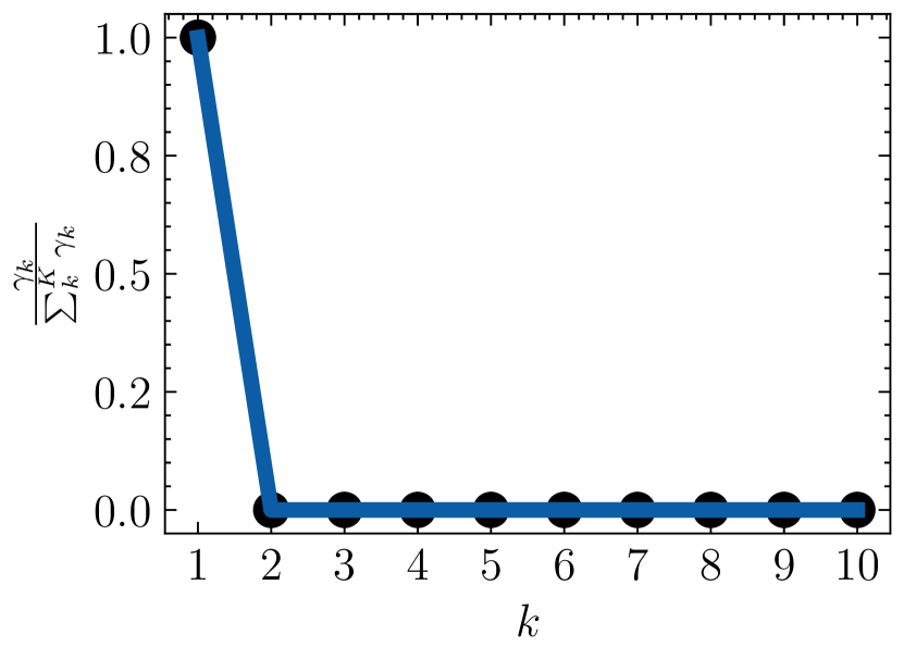
(a) $N=100$.

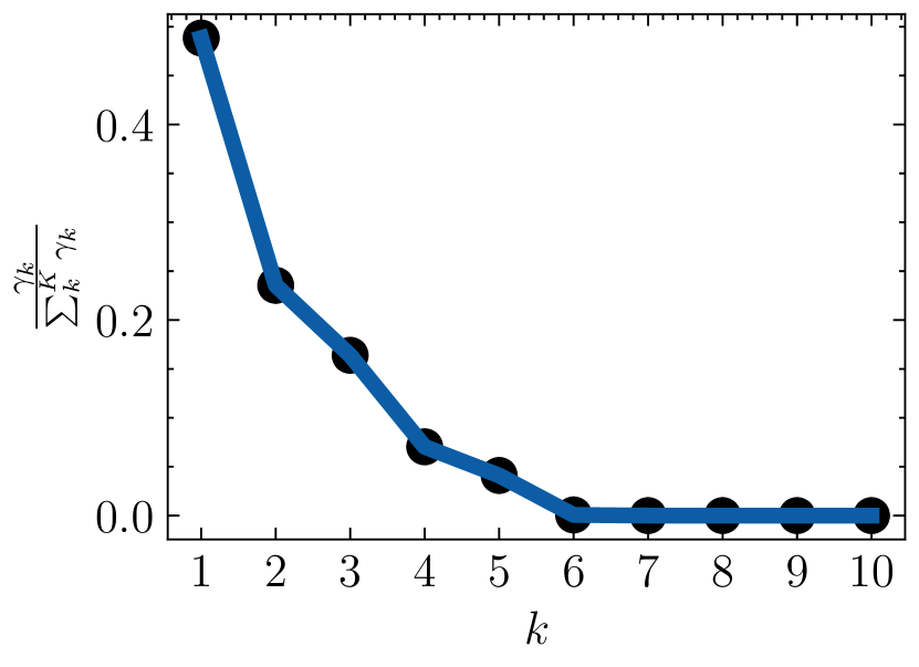
(b) $N=500$.

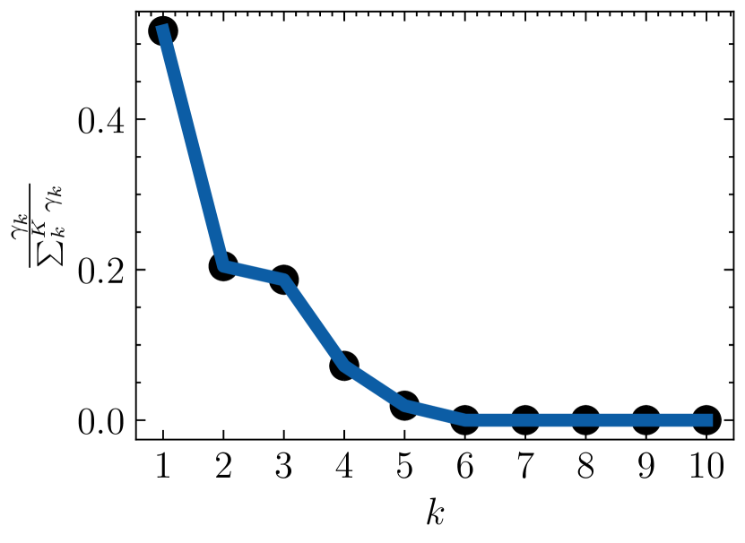
(c) $N=1000$.

Figure 18: Eigenvalues decay for problem P3.

5 Conclusion and Future Work

In this paper, we proposed modifications to the classical RBF-NN model, to enhance its interpretability and uncover the underlying factors of variation known as the active subspace. Our approach involved incorporating a learnable precision matrix into the Gaussian kernel, allowing us to extract latent information about the prediction task from the eigenvectors and eigenvalues.

Our extensive numerical experiments covered regression, classification, and feature selection tasks, where we compared our proposed model with widely used methods such as SVM, RF, GB, and state-of-the-art deep learning-based embedding methods. The results demonstrated that our GRBF-NN model achieved attractive prediction performance while providing meaningful feature importance rankings. One of the key observations from our experiments was the impact of the regularizer $\lambda_{\mathbf{u}}$ on the performance of the GRBF-NN, which often prevails the effect of the weight regularizer $\lambda_{\mathbf{w}}$. This finding suggests that prioritizing the regularization of the precision matrix yields more significant improvements in the model generalization performance.

By combining predictive power with interpretability, the GRBF-NN offers a valuable tool for understanding complex nonlinear relationships in the data. Moreover, the model enables supervised dimensionality reduction, facilitating visualization and comprehension of complex phenomena. Overall, our work contributes to bridging the gap between black-box neural network models and interpretable machine learning, enabling users to not only make accurate predictions but also gain meaningful insights from the model behavior and improve decision-making processes in real-world applications.

Looking ahead, we plan to apply our model to tackle the so-called curse of dimensionality in expensive engineering optimization problems. By leveraging the active subspace estimation, we aim to reduce the dimensionality of optimization problems without relying on direct gradient computations as in the classical ASM, which is not desirable in noisy gradient scenarios.

References

- [1] Amina Adadi and Mohammed Berrada. Peeking inside the black-box: a survey on explainable artificial intelligence (xai). IEEE access, 6:52138–52160, 2018.
- [2] Kofi P Adragni and R Dennis Cook. Sufficient dimension reduction and prediction in regression. Philosophical Transactions of the Royal Society A: Mathematical, Physical and Engineering Sciences, 367(1906):4385–4405, 2009.
- [3] Stefan Aeberhard, Danny Coomans, and Olivier De Vel. Comparative analysis of statistical pattern recognition methods in high dimensional settings. Pattern Recognition, 27(8):1065–1077, 1994.
- [4] Fevzi Alimoglu and Ethem Alpaydin. Methods of combining multiple classifiers based on different representations for pen-based handwriting recognition. In Proceedings of the fifth Turkish artificial intelligence and artificial neural networks symposium (TAINN 96), 1996.
- [5] Alejandro Barredo Arrieta, Natalia Díaz-Rodríguez, Javier Del Ser, Adrien Bennetot, Siham Tabik, Alberto Barbado, Salvador García, Sergio Gil-López, Daniel Molina, Richard Benjamins, et al. Explainable artificial intelligence (xai): Concepts, taxonomies, opportunities and challenges toward responsible ai. Information fusion, 58:82–115, 2020.
- [6] Richard Bellman. Dynamic programming. Science, 153(3731):34–37, 1966.
- [7] Yoshua Bengio, Aaron Courville, and Pascal Vincent. Representation learning: A review and new perspectives. IEEE transactions on pattern analysis and machine intelligence, 35(8):1798–1828, 2013.
- [8] Yue Bi, Dongxu Xiang, Zongyuan Ge, Fuyi Li, Cangzhi Jia, and Jiangning Song. An interpretable prediction model for identifying n7-methylguanosine sites based on xgboost and shap. Molecular Therapy-Nucleic Acids, 22:362–372, 2020.
- [9] Chris Bishop. Improving the generalization properties of radial basis function neural networks. Neural computation, 3(4):579–588, 1991.
- [10] Christopher M Bishop. Curvature-driven smoothing in backpropagation neural networks. In Theory and Applications of Neural Networks, pages 139–148. Springer, 1992.
- [11] Christopher M Bishop et al. Neural networks for pattern recognition. Oxford university press, 1995.
- [12] Leo Breiman. Random forests. Machine learning, 45(1):5–32, 2001.
- [13] David S Broomhead and David Lowe. Radial basis functions, multi-variable functional interpolation and adaptive networks. Technical report, Royal Signals and Radar Establishment Malvern (United Kingdom), 1988.
- [14] Jianbo Chen, Mitchell Stern, Martin J Wainwright, and Michael I Jordan. Kernel feature selection via conditional covariance minimization. Advances in Neural Information Processing Systems, 30, 2017.
- [15] Paul G Constantine, Eric Dow, and Qiqi Wang. Active subspace methods in theory and practice: applications to kriging surfaces. SIAM Journal on Scientific Computing, 36(4):A1500–A1524, 2014.
- [16] R Dennis Cook. On the interpretation of regression plots. Journal of the American Statistical Association, 89(425):177–189, 1994.
- [17] R Dennis Cook. Regression graphics: Ideas for studying regressions through graphics. John Wiley & Sons, 2009.
- [18] Corinna Cortes and Vladimir Vapnik. Support-vector networks. Machine learning, 20:273–297, 1995.
- [19] David Deterding. Speaker normalization for automatic speech recognition. University of Cambridge, Ph. D. Thesis, 1989.
- [20] Abhirup Dikshit and Biswajeet Pradhan. Interpretable and explainable ai (xai) model for spatial drought prediction. Science of the Total Environment, 801:149797, 2021.
- [21] Dheeru Dua and Casey Graff. UCI machine learning repository, 2017.
- [22] Danny D’Agostino, Andrea Serani, and Matteo Diez. Design-space assessment and dimensionality reduction: An off-line method for shape reparameterization in simulation-based optimization. Ocean Engineering, 197:106852, 2020.
- [23] Ian W. Evett and E. J. Spiehler. Rule induction in forensic science. In KBS in Government, pages 107–118. Online Publications, 1987.
- [24] Ronald A Fisher. The use of multiple measurements in taxonomic problems. Annals of eugenics, 7(2):179–188, 1936.
- [25] Jerome H Friedman. Multivariate adaptive regression splines. The annals of statistics, 19(1):1–67, 1991.
- [26] Jerome H Friedman. Greedy function approximation: a gradient boosting machine. Annals of statistics, pages 1189–1232, 2001.
- [27] Kunihiko Fukushima. Cognitron: A self-organizing multilayered neural network. Biological cybernetics, 20(3-4):121–136, 1975.
- [28] Federico Girosi, Michael Jones, and Tomaso Poggio. Regularization theory and neural networks architectures. Neural computation, 7(2):219–269, 1995.
- [29] Riccardo Guidotti, Anna Monreale, Salvatore Ruggieri, Franco Turini, Fosca Giannotti, and Dino Pedreschi. A survey of methods for explaining black box models. ACM computing surveys (CSUR), 51(5):1–42, 2018.
- [30] Isabelle Guyon and André Elisseeff. An introduction to variable and feature selection. Journal of machine learning research, 3(Mar):1157–1182, 2003.
- [31] Trevor Hastie, Robert Tibshirani, Jerome H Friedman, and Jerome H Friedman. The elements of statistical learning: data mining, inference, and prediction, volume 2. Springer, 2009.
- [32] Katja Hauser, Alexander Kurz, Sarah Haggenmüller, Roman C Maron, Christof von Kalle, Jochen S Utikal, Friedegund Meier, Sarah Hobelsberger, Frank F Gellrich, Mildred Sergon, et al. Explainable artificial intelligence in skin cancer recognition: A systematic review. European Journal of Cancer, 167:54–69, 2022.
- [33] Kurt Hornik, Maxwell Stinchcombe, and Halbert White. Multilayer feedforward networks are universal approximators. Neural networks, 2(5):359–366, 1989.
- [34] Harold Hotelling. Analysis of a complex of statistical variables into principal components. Journal of educational psychology, 24(6):417, 1933.
- [35] Jennifer L Jefferson, James M Gilbert, Paul G Constantine, and Reed M Maxwell. Active subspaces for sensitivity analysis and dimension reduction of an integrated hydrologic model. Computers & geosciences, 83:127–138, 2015.
- [36] https://www.kaggle.com/datasets/mahirkukreja/delhi-weather-data.
- [37] Diederik P Kingma and Jimmy Ba. Adam: A method for stochastic optimization. arXiv preprint arXiv:1412.6980, 2014.
- [38] Ker-Chau Li. Sliced inverse regression for dimension reduction. Journal of the American Statistical Association, 86(414):316–327, 1991.
- [39] Yifeng Li, Chih-Yu Chen, and Wyeth W Wasserman. Deep feature selection: theory and application to identify enhancers and promoters. Journal of Computational Biology, 23(5):322–336, 2016.
- [40] Tyson Loudon and Stephen Pankavich. Mathematical analysis and dynamic active subspaces for a long term model of hiv. arXiv preprint arXiv:1604.04588, 2016.
- [41] Trent W Lukaczyk, Paul Constantine, Francisco Palacios, and Juan J Alonso. Active subspaces for shape optimization. In 10th AIAA multidisciplinary design optimization conference, page 1171, 2014.
- [42] Scott M Lundberg and Su-In Lee. A unified approach to interpreting model predictions. Advances in neural information processing systems, 30, 2017.
- [43] James McDermott and Richard S. Forsyth. Diagnosing a disorder in a classification benchmark. Pattern Recognition Letters, 73:41–43, 2016.
- [44] Charles A Micchelli. Interpolation of scattered data: distance matrices and conditionally positive definite functions. In Approximation theory and spline functions, pages 143–145. Springer, 1984.
- [45] Michael Mongillo et al. Choosing basis functions and shape parameters for radial basis function methods. SIAM undergraduate research online, 4(190-209):2–6, 2011.
- [46] John Moody and Christian J Darken. Fast learning in networks of locally-tuned processing units. Neural computation, 1(2):281–294, 1989.
- [47] David W Nierenberg, Therese A Stukel, John A Baron, Bradley J Dain, E Robert Greenberg, and Skin Cancer Prevention Study Group. Determinants of plasma levels of beta-carotene and retinol. American Journal of Epidemiology, 130(3):511–521, 1989.
- [48] Jean Jacques Ohana, Steve Ohana, Eric Benhamou, David Saltiel, and Beatrice Guez. Explainable ai (xai) models applied to the multi-agent environment of financial markets. In International Workshop on Explainable, Transparent Autonomous Agents and Multi-Agent Systems, pages 189–207. Springer, 2021.
- [49] R Kelley Pace and Ronald Barry. Sparse spatial autoregressions. Statistics & Probability Letters, 33(3):291–297, 1997.
- [50] Jooyoung Park and Irwin W Sandberg. Universal approximation using radial-basis-function networks. Neural computation, 3(2):246–257, 1991.
- [51] Jooyoung Park and Irwin W Sandberg. Approximation and radial-basis-function networks. Neural computation, 5(2):305–316, 1993.
- [52] Adam Paszke, Sam Gross, Francisco Massa, Adam Lerer, James Bradbury, Gregory Chanan, Trevor Killeen, Zeming Lin, Natalia Gimelshein, Luca Antiga, Alban Desmaison, Andreas Kopf, Edward Yang, Zachary DeVito, Martin Raison, Alykhan Tejani, Sasank Chilamkurthy, Benoit Steiner, Lu Fang, Junjie Bai, and Soumith Chintala. Pytorch: An imperative style, high-performance deep learning library. In Advances in Neural Information Processing Systems 32, pages 8024–8035. Curran Associates, Inc., 2019.
- [53] Karl Pearson. On lines and planes of closest fit to systems of points in space. The London, Edinburgh, and Dublin Philosophical Magazine and Journal of Science, 2(11):559–572, 1901.
- [54] F. Pedregosa, G. Varoquaux, A. Gramfort, V. Michel, B. Thirion, O. Grisel, M. Blondel, P. Prettenhofer, R. Weiss, V. Dubourg, J. Vanderplas, A. Passos, D. Cournapeau, M. Brucher, M. Perrot, and E. Duchesnay. Scikit-learn: Machine learning in Python. Journal of Machine Learning Research, 12:2825–2830, 2011.
- [55] Keith W Penrose, AG Nelson, and AG Fisher. Generalized body composition prediction equation for men using simple measurement techniques. Medicine & Science in Sports & Exercise, 17(2):189, 1985.
- [56] Tomaso Poggio and Federico Girosi. Networks for approximation and learning. Proceedings of the IEEE, 78(9):1481–1497, 1990.
- [57] MJD Powell. Radial basis function methods for interpolation to functions of many variables. In HERCMA, pages 2–24. Citeseer, 2001.
- [58] Marco Tulio Ribeiro, Sameer Singh, and Carlos Guestrin. " why should i trust you?" explaining the predictions of any classifier. In Proceedings of the 22nd ACM SIGKDD international conference on knowledge discovery and data mining, pages 1135–1144, 2016.
- [59] Friedhelm Schwenker, Hans A Kestler, and Günther Palm. Three learning phases for radial-basis-function networks. Neural networks, 14(4-5):439–458, 2001.
- [60] Jack W Smith, James E Everhart, WC Dickson, William C Knowler, and Robert Scott Johannes. Using the adap learning algorithm to forecast the onset of diabetes mellitus. In Proceedings of the annual symposium on computer application in medical care, page 261. American Medical Informatics Association, 1988.
- [61] Thomas A Stamey, John N Kabalin, John E McNeal, Iain M Johnstone, Fuad Freiha, Elise A Redwine, and Norman Yang. Prostate specific antigen in the diagnosis and treatment of adenocarcinoma of the prostate. ii. radical prostatectomy treated patients. The Journal of urology, 141(5):1076–1083, 1989.
- [62] W Nick Street, William H Wolberg, and Olvi L Mangasarian. Nuclear feature extraction for breast tumor diagnosis. In Biomedical image processing and biomedical visualization, volume 1905, pages 861–870. SPIE, 1993.
- [63] Robert Tibshirani. Regression shrinkage and selection via the lasso: a retrospective. Journal of the Royal Statistical Society: Series B (Statistical Methodology), 73(3):273–282, 2011.
- [64] Dietrich Wettschereck and Thomas Dietterich. Improving the performance of radial basis function networks by learning center locations. Advances in neural information processing systems, 4, 1991.
- [65] Maksymilian Wojtas and Ke Chen. Feature importance ranking for deep learning. Advances in Neural Information Processing Systems, 33:5105–5114, 2020.
- [66] Xiang Yi Wong, Yu Kai Ang, Keqi Li, Yip Han Chin, Sean Shao Wei Lam, Kenneth Boon Kiat Tan, Matthew Chin Heng Chua, Marcus Eng Hock Ong, Nan Liu, Ahmad Reza Pourghaderi, et al. Development and validation of the sarica score to predict survival after return of spontaneous circulation in out of hospital cardiac arrest using an interpretable machine learning framework. Resuscitation, 170:126–133, 2022.
- [67] I-Cheng Yeh, King-Jang Yang, and Tao-Ming Ting. Knowledge discovery on rfm model using bernoulli sequence. Expert Systems with Applications, 36(3, Part 2):5866–5871, 2009.