CILF:Causality Inspired Learning Framework for Out-of-Distribution Vehicle Trajectory Prediction

Abstract

Trajectory prediction is critical for autonomous driving vehicles. Most existing methods tend to model the correlation between history trajectory (input) and future trajectory (output). Since correlation is just a superficial description of reality, these methods rely heavily on the i.i.d. assumption and evince a heightened susceptibility to out-of-distribution data. To address this problem, we propose an Out-of-Distribution Causal Graph (OOD-CG), which explicitly defines the underlying causal structure of the data with three entangled latent features: 1) domain-invariant causal feature (IC), 2) domain-variant causal feature (VC), and 3) domain-variant non-causal feature (VN). While these features are confounded by confounder (C) and domain selector (D). To leverage causal features for prediction, we propose a Causal Inspired Learning Framework (CILF), which includes three steps: 1) extracting domain-invariant causal feature by means of an invariance loss, 2) extracting domain variant feature by domain contrastive learning, and 3) separating domain-variant causal and non-causal feature by encouraging causal sufficiency. We evaluate the performance of CILF in different vehicle trajectory prediction models on the mainstream datasets NGSIM and INTERACTION. Experiments show promising improvements in CILF on domain generalization.

1 Introduction

Trajectory prediction is essential for both the perception and planning modules of autonomous vehicles [19, 12] in order to reduce the risk of collisions [13]. Recent trajectory prediction methods are primarily built with deep neural networks, which are trained to model the correlation between history trajectory and future trajectory. The robustness of such correlation is guaranteed by the independent and identically distributed (i.i.d.) assumption. As a result, the model trained on i.i.d. samples often fails to be generalized to out-of-distribution (OOD) samples.

Recently, there has been a growing interest in utilizing causal representation learning [25] to tackle the challenge of out-of-domain generalization [32]. Causal representation learning is based on the Structure Causal Model (SCM) [7, 20], a mathematical tool for modeling human metaphysical concepts about causation. Causal representation learning enables the model to discern the underlying causal structure of data by incorporating causal-related prior knowledge into the model.

This paper proposes an Out-of-Distribution Causal Graph (OOD-CG) based on SCM, as shown in Fig.1. OOD-DG divides the latent features into three categories: 1) Domain-invariant Causal Feature (IC) such as physical laws, driving habits, etc. 2) Domain-variant Causal Feature (VC) such as road traffic flow, traffic scenes, etc. 3) Domain-variant Non-causal Feature (VN) like sensor noise, etc. These features are entangled due to the confounding effects of backdoor confounder (C) and domain selector (D).

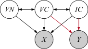
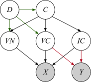
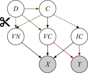
Figure 1: The step-by-step introduction of OOD-CG. White nodes represent latent features; gray nodes represent observable variables; bidirectional arrows represent correlations; unidirectional arrows represent causal mechanisms; red arrows represent causal mechanisms critical to prediction; and green arrows represent domain effects.

To leverage causal features for trajectory prediction, we introduce a Causal-Inspired Learning Framework (CILF) based on causal representation learning. CILF includes three parts to block the backdoor paths associated with IC, VC, and VN. First, to block the backdoor path between IC and domain-variant feature V, CILF utilizes invariant risk minimization (IRM) [2] to extract IC and domain contrastive learning [10] to extract V. Then, to block the backdoor path between VC and VN, CILF introduces domain adversarial learning [9] to separate VC and VN.

Our contributions can be summarized as follows:

(1) We propose a theoretical model named OOD-CG, which explicitly elucidates the causal mechanisms and causal structure of the out-of-distribution generalization problem.

(2) Based on causal representation learning, we propose a learning framework called CILF for out-of-distribution vehicle trajectory prediction. CILF contains three steps to block the backdoor connection associated with IC, VC, and VN, allowing the model to employ causal features for prediction.

2 Related Work

2.0.1 Vehicle trajectory Prediction

Recent works widely employ the sequence-to-sequence (Seq2seq) framework [26] to predict a vehicle’s future trajectory based on its history trajectory [1, 5, 11, 27]. Alahi et al. introduce S-LSTM [1], which incorporates a social pooling mechanism to aggregate and encode the social behaviors of surrounding vehicles. Deo et al. propose CS-LSTM [5], which utilizes convolutional operations to enhance the model’s performance. Lee et al. introduce a trajectory prediction model called DESIRE [11], which combines conditional variational auto-encoder (CVAE) and GRU to generate multimodal predictions of future trajectories. Tang et al. incorporate an attention mechanism into the Seq2seq framework named MFP [27], a model that can effectively learn motion representations of multiple vehicles across multiple time steps. However, current vehicle trajectory prediction approaches still face the challenge of OOD generalization, posing a serious threat to the safety of autonomous vehicles.

2.0.2 Out-of-Distribution generalization

Previous methods handle OOD generalization in two paradigms: domain adaptation (DA) and domain generalization (DG) [32]. DA allows the model to access a small portion of unlabeled target domain data during training, thereby reducing the difficulty of the OOD problem to some extent. DA aims to learn an embedding space where source domain samples and target domain samples follow similar distributions via minimizing divergence [8, 15], domain adversarial learning [6, 28], etc. DG prohibits models from accessing any form of target domain data during training. DG aims to learn knowledge that can be directly transferred to unknown target domains. Relevant literature has proposed a range of solutions, including contrastive learning [17, 29], domain adversarial learning [28, 31], etc. As for vehicle trajectory prediction, it is difficult to acquire even unlabeled target domain samples. As a result, we follow the paradigm of domain generalization.

2.0.3 Causality inspired approaches for domain generalization

There has been a growing trend toward utilizing causality inspired methods to address the OOD problem. Some of them suggest using mathematical formulas from causal inference [20], e.g.,front-door adjustment [18] and back-door adjustment [3] formulas, to directly derive the loss function. However, these methods often make strong assumptions (e.g.,restricting the model to be a variational auto-encoder [3]), which decrease the diversity of the model’s hypothesis space and limit the applicability of the model. Some approaches instead only make assumptions about the general causal structure of the OOD problem in order to guide the design of network structures [14, 16]. We follow this approach in order to enhance the versatility of the proposed model.

3 Theoretical Analysis

3.1 Problem Formulation

We formulated vehicle trajectory prediction as estimating future trajectories $Y_{i}=\{(x_{i,t},y_{i,t})\in\mathbb{R}^{2}|t=t_{obs}+1,...,t_{pred}\}$ based on the observed history trajectories $X_{i}=\{(x_{i,t},y_{i,t})\in\mathbb{R}^{2}|t=1,2,...,t_{obs}\}$ of $N$ visible vehicles in the current scene. In the context of domain generalization, the training dataset is collected from $K$ source domains, denoted as $S\in\{S_{1},S_{2},...,S_{K}\}$, while the test dataset is collected from $M$ target domains, denoted as $T\in\{T_{1},T_{2},...,T_{M}\}$.

3.2 OOD-CG

Fig.1. Traditional deep learning is designed to capture statistical correlations between inputs $X$ and outputs $Y$. Correlations are obviously inadequate to solve the OOD problem. Fortunately, Reichenbach provides us with a strong tool called the common causal principle [23] to decompose these correlations into a set of backdoor features.

Theorem 3.1

Common causal principle: if two random variables $X$ and $Y$ are correlated, there must exist another random variable $S$ that has causal relationships with both $X$ and $Y$. Furthermore, $S$ can completely substitute for the correlations between $X$ and $Y$, i.e., $X\perp\!\!\!\perp Y|S$.

Fig.1. We divide these backdoor features into three classes: (1) Domain-Invariant Causal Feature (IC): Driving habits, physical laws, etc. (2) Domain-Variant Causal Feature (VC): Traffic density, traffic scenario, etc. (3) Domain-Variant Non-causal Feature (VN): Sensor measurement noise, etc. Bidirectional arrows are used in this step to represent the entanglement between these backdoor features. Previous studies often ignore domain-variant causal feature VC, and focus solely on utilizing domain-invariant causal feature IC for prediction [3, 4, 18]. These approaches utilize insufficient causal information for prediction and thus fail to simultaneously improve prediction accuracy in both the source and target domains.

Fig.1. According to Theorem.3.1, we introduce a Confounder (C) to summarize all the correlations among IC, VC, and VN. We also introduce a Domain Selector (D) to represent domain effects. Since domain label is unavailable during testing, we treat D as an unobservable latent variable consistent with  [3, 16]. Now we can concretize distribution shifts as differences in feature prior distributions $P(C),P(VC),P(VN)$ and causal mechanism conditional distributions $P(VC|C),P(VN|C)$ between source and target domains.

Fig.1. In order to extract domain-invariant causal mechanisms $P(Y|VC)$, $P(Y|IC)$ for prediction, it is necessary to block the backdoor paths connecting these entangled features. To do so, we only need to block the backdoor paths of IC and VN, which are represented by dashed lines in the figure. Once done, VC actually serves as a mediator [7, 20] in causal effects from D and C to Y, which can be completely substituted by VC. In the next chapter, we introduce a causal-inspired learning framework (CILF) for OOD vehicle trajectory prediction, encouraging models to block the backdoor paths of IC and VN.

4 CILF

Compared to traditional machine learning, deep learning requires searching within an extremely complex hypothesis space. As a result, researchers often introduce inductive bias into deep learning models to reduce search difficulty, allowing models to find some relatively acceptable local optimums within limited training iterations. OOD-CG is proposed to impose such inductive bias theoretically. Guided by OOD-CG, we propose CILF (see Fig.2) to extract causal features for prediction. First, to block the backdoor connection between IC and V, CILF introduces two kinds of losses: IRM loss to encourage domain-invariant causal feature IC; Domain contrastive loss to encourage domain-variant feature V. Then, to block the backdoor path between VC and VN, CILF introduces domain adversarial learning to train a mask generator able to detect the causal dimensions VC and non-causal dimensions VN of domain-variant feature V.

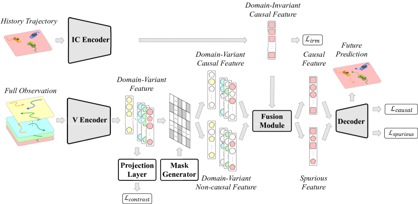
Figure 2: CILF consists of three parts: (i)IC encoder $\Phi_{ic}(.)$ takes history trajectories of the current vehicle as input. The IRM loss $\mathcal{L}_{irm}$ is utilized to encourage the extracted feature to exhibit domain invariance; (ii)Domain-variant feature encoder $\Phi_{v}(.)$ takes full observations from each source domain as input, such as history trajectories of neighboring vehicles, map information, etc. The domain contrastive learning loss $\mathcal{L}_{contrast}$ is utilized to encourage the extracted feature to exhibit domain variance; (iii)Mask generator $M(.)$ generates a causally sufficient mask to select the causal dimensions VC and non-causal dimensions VN from V.

4.1 Extract Domain-invariant Causal Feature

Domain-invariant features are the intersection of feature sets from different domains. The non-causal information within these features exhibits a significant reduction after taking the intersection. As a result, extracting IC can be approximated as extracting the domain-invariant feature. The definition of a domain-invariant encoder is given as follows [2]:

Definition 1

Domain-invariant feature encoder: An encoder $\Phi(.):\mathcal{X}\to\mathcal{H}$ is said to be a domain-invariant encoder across all domains $s\in S$ if and only if there exists a decoder $\Theta(.):\mathcal{H}\to\mathcal{Y}$ that achieves optimum across all domains. This condition can be further formulated as a conditional optimization problem:

$$\begin{split}&\underset{\Phi,\Theta}{\mathrm{min}}\Sigma_{s\in S}\mathcal{L}_{s}(\Theta\circ\Phi),\\ \text{subject to }\Theta\in&\underset{\bar{\Theta}}{\mathrm{argmin}}\mathcal{L}_{s}(\bar{\Theta}\circ\Phi),\text{for all }s\in S.\end{split}$$ (1)

However, this is a bi-level optimization problem, which is computationally difficult to solve. In current research, the problem is often relaxed to a gradient regularization penalty based on empirical risk minimization [2]:

$$\underset{\Phi_{IC},\Theta}{\mathrm{min}}\frac{1}{\lvert S\rvert}\Sigma_{s\in S}[\mathcal{L}_{s}(\Theta\circ\Phi_{IC})+\lambda\lVert\nabla_{\Theta}\mathcal{L}_{s}(\Theta\circ\Phi_{IC})\rVert^{2}],$$ (2)

$$\mathcal{L}_{irm}=\frac{1}{\lvert S\rvert}\lVert\nabla_{\Theta}\mathcal{L}_{s}(\Theta\circ\Phi_{IC})\rVert^{2},$$ (3)

where $\mathcal{L}_{irm}$ denotes the IRM loss, $\lambda$ denotes the balance parameter.

We separate $\Phi_{IC}$ from the backbone to further block the backdoor path of IC, as shown in Fig.2. $\Phi_{IC}$ only accepts the history trajectories of the current vehicle as input, which contains relatively limited domain knowledge.

4.2 Extract Domain-variant Feature

To extract domain-variant feature, we design $\Phi_{v}(.)$, which takes full observations from different domains (distinguished by the colors in Fig.2) as input. Full observations include all the information that an autonomous driving vehicle can observe in a traffic scene (e.g., history trajectories of neighboring vehicles, map information, etc.), which are highly domain-related. $\Phi_{v}(.)$ is trained using domain contrastive loss [10, 14]. In order to calculate this loss, CILF employs dimensional reduction to V through a projection layer $p_{i}=\beta(V_{i})$, where $i$ denotes the domain label. The contrastive loss between a pair of samples $p_{i}$ and $p_{j}$ is defined as follows:

$$\mathcal{L}_{contrast}=-\mathrm{log}\frac{\mathrm{exp}(p_{i},p_{j})/\tau}{\Sigma_{k}\mathbb{I}_{[k=j\lor S_{k}\neq S_{i}]}\mathrm{exp}(\mathrm{sim}(p_{i},p_{k})/\tau)}$$ (4)

where $\mathbb{I}_{[k=j\lor S_{k}\neq S_{i}]}$ denotes the indicator function. When sample $p_{i}$ and $p_{k}$ are from the same domain, this function equals to 1. $\tau$ is the temperature parameter of contrastive learning, $\mathrm{sim}(a,b)=\frac{a^{\mathrm{T}}b}{\lVert a\rVert\lVert b\rVert}$ is the cosine similarity.

4.3 Separate Domain-variant Causal and Non-causal Feature

In Section 4.1, we argue that domain-invariant features naturally possess causality as they are the intersection of feature sets from different domains. However, domain-variant features do not naturally carry this causal property. It is necessary to filter out the non-causal dimensions within these features according to causal sufficiency [21, 23, 24]:

Definition 2

Causally sufficient feature set: for the prediction task from $X$ to $Y$, a feature set is considered causally sufficient if and only if it captures all causal effects from $X$ to $Y$.

Supervised learning can’t guarantee the learned features to be causally sufficient according to Definition.2. Some dimensions may contain more causal information and have a decisive impact on prediction, while other dimensions may have little influence on prediction. CILF introduces a neural network based mask generator $M(.)$ that produces a causally sufficient mask [16] using the Gumbel-SoftMax technique [9]:

$$m=\mathrm{Gumbel-SoftMax}(M(V),kN),$$ (5)

The causally sufficient mask can identify the contribution $k\in(0,1)$ of each dimension in V to prediction. The top $kN$ dimensions with the highest contributions are regarded as domain-variant causal features VC, while the remaining dimensions are considered domain-variant non-causal features VN:

$$\textit{VC}=V\cdot m,\textit{VN}=V\cdot(1-m).$$ (6)

VC and VN are fused with IC by the fusion module $F(.)$ to form causal features CF and spurious features SF, which are then decoded separately by $\Theta(.)$ to generate future predictions. Prediction losses $\mathcal{L}_{causal}$ and $\mathcal{L}_{spurious}$ can be calculated by RMSE:

$$\begin{split}CF=F(VC,IC)&=f_{2}(f_{1}(VC,IC)+IC),\\ SF=F(VN,IC)&=f_{2}(f_{1}(VN,IC)+IC),\end{split}$$ (7)

$$\begin{split}\mathcal{L}_{causal}&=\mathrm{RMSE}(\Theta(VC),Y),\\ \mathcal{L}_{spurious}&=\mathrm{RMSE}(\Theta(VN),Y),\end{split}$$ (8)

where $f_{1}$ and $f_{2}$ are FC layers in fusion module.

Decoder $\Theta$ can be trained by minimizing $\mathcal{L}_{causal}$ and $\mathcal{L}_{spurious}$. Mask generator $M$ can be trained by minimizing $\mathcal{L}_{causal}$ while adversarially maximizing $\mathcal{L}_{spurious}$. Overall, the optimization objective can be formulated as follows:

$$\underset{\Phi_{IC},F,\Theta}{\mathrm{min}}\mathcal{L}_{causal}+\mathcal{L}_{spurious}+\lambda\mathcal{L}_{irm}$$ (9)

$$\underset{\Phi_{v},F,\Theta}{\mathrm{min}}\mathcal{L}_{causal}+\mathcal{L}_{spurious}+\alpha\mathcal{L}_{irm}$$ (10)

$$\underset{M}{\mathrm{min}}\mathcal{L}_{causal}-\mathcal{L}_{spurious}$$ (11)

where $\lambda$ and $\alpha$ are balance parameters.

5 Experiments

This chapter presents quantitative and qualitative domain generalization experiments of the proposed CILF framework on the public vehicle trajectory prediction datasets NGSIM [22] and INTERACTION [30].

5.1 Experiment Design

INTERACTION is a large-scale real-world dataset that includes top-down vehicle trajectory data in three scenarios: intersections, highway ramps (referred to as merging), and roundabouts, collected from multiple locations in America, Asia, and Europe. INTERACTION consists of 11 subsets, categorized into three types of scenarios: roundabouts, highway ramps, and intersections (see Table 1). NGSIM is a collection of vehicle trajectory data derived from video recordings. It includes vehicle trajectory data from three different locations: the US-101 highway, Lankershim Blvd. in Los Angeles, and the I-80 highway in Emeryville. The sampling rate of both datasets is 10Hz. For each trajectory that lasts 8 seconds, the model takes the first 3 seconds as input and predicts the trajectory for the next 5 seconds.

As shown in Table 1, data volume among different subsets of INTERACTION varies significantly. Subsets 0, 1, and 7 have notably higher data volumes compared to other subsets. To mitigate the potential influence of data volume disparities, we design three contrastive experiments to demonstrate the effectiveness of CILF in addressing the DG problem:

Table 1: INTERACTION Dataset. Data Ratio represents the proportion of data volume in each subset relative to the total data volume.

Subset ID	Sample Location	Scenario	Data Ratio
0	USA	Roundabout	17.9%
1	CHN	Merging	35.2%
2	USA	Intersection	7.9%
3	USA	Intersection	2.6%
4	GER	Roundabout	1.8%
5	USA	Roundabout	5.3%
6	GER	Merging	1.2%
7	USA	Intersection	21.6%
8	USA	Roundabout	3.2%
9	USA	Intersection	2.6%
10	CHN	Roundabout	0.6%

(1)Single-scenario domain generalization: Both training and test datasets come from the same scenario within the INTERACTION. Specifically, the subset with the largest data volume in each scenario is designated as the test set, while the remaining subsets serve as the training set.

(2)Cross-scenario domain generalization: The training and test datasets come from different scenarios within the INTERACTION. Specifically, the three subsets with the largest data volumes (roundabout-0, merging-1, and intersection-7) are selected as training sets, while the remaining subsets are chosen as test sets.

(3)Cross-dataset domain generalization: The INTERACTION is selected as the training set, while the NGSIM is selected as the test set.

We choose three classic vehicle trajectory prediction models as baselines:

S-LSTM [1]:An influential method based on a social pooling model;

CS-LSTM [5]:A model using a convolutional social pooling structure to learn vehicle interactions;

MFP [27]:An advanced model that learns semantic latent variables for trajectory prediction. These baselines are trained under CILF to compare their domain generalization performance.

We employ two commonly used metrics in vehicle trajectory prediction to measure the model’s domain generalization performance:

Average Displacement Error (ADE): Average L2 distance between predicted points and groundtruth points across all timesteps.

$$\mathrm{ADE}=\frac{\Sigma_{i=1}^{N}\Sigma_{t=t_{obs}+1}^{t_{pred}}\lVert\hat{Y}_{i,t}-Y_{i,t}\rVert}{N},$$ (12)

Final Displacement Error (FDE): L2 distance between predicted points and ground truth points at the final timestep.

$$\mathrm{FDE}=\frac{\Sigma_{i=1}^{N}\lVert\hat{Y}_{i,t}-Y_{i,t}\rVert}{N},t=t_{obs}+1,...,t_{pred}.$$ (13)

5.2 Quantitative Experiment and Analysis

5.2.1 Single-scenario domain generalization

Table 2 and Table 3 present the comparison between different models trained under CILF and vanilla conditions in terms of single-scenario domain generalization on the INTERACTION.

Table 2: ADE and FDE (in meters) results of domain generalization experiment in the intersection scenario. Subset 7 is left for testing, while other subsets of the intersection scenario are used for training.

	S-LSTM		CS-LSTM		MFP
	ADE	FDE	ADE	FDE	ADE	FDE
Intersection-2	1.52/1.59	4.65/4.85	1.53/1.64	4.62/4.86	1.62/1.72	5.05/5.29
Intersection-3	1.21/1.29	3.48/3.60	1.18/1.28	3.43/3.59	1.25/1.32	3.67/3.83
Intersection-9	1.20/1.29	3.37/3.53	1.20/1.30	3.36/3.56	1.25/1.34	3.57/3.79
Intersection-7	2.22/2.25	6.20/6.32	2.34/2.37	6.30/6.47	2.12/2.21	6.02/6.04

Table 3: ADE and FDE (in meters) results of domain generalization experiment in the roundabout scenario. Subset 0 is left for testing, while other subsets of the roundabout scenario are used for training.

	S-LSTM		CS-LSTM		MFP
	ADE	FDE	ADE	FDE	ADE	FDE
Roundabout-4	1.68/1.75	4.41/4.64	1.62/1.83	4.41/4.81	1.59/1.73	2.86/3.14
Roundabout-6	1.03/1.12	2.97/3.09	1.01/1.10	2.86/3.02	1.01/1.14	2.86/3.14
Roundabout-10	1.42/1.57	3.60/3.94	1.38/1.51	3.50/3.94	1.30/1.60	3.42/4.05
Roundabout-0	3.31/3.34	9.04/9.38	3.24/3.35	9.01/9.09	3.15/3.25	8.80/8.83

CILF achieves both ADE and FDE improvements for all models in both the source and target domains.

In the intersection scenario, as shown in Table 2, for the source domains, CS-LSTM achieves the largest improvement under CILF, with average increments of 7.40% and 5.00% (ADE and FDE). Conversely, S-LSTM shows the lowest improvement, with average increments of 5.86% and 4.00%. As for the target domain, S-LSTM and MFP demonstrate similar improvements, with increments of 1.33%, 1.90% for S-LSTM and 1.40%, 1.33% for MFP.

In the roundabout scenario, as shown in Table 3, for the source domains, MFP achieves the largest improvement under CILF, with average increments of 12.75% and 9.31% (ADE and FDE). Conversely, S-LSTM shows the lowest improvement, with average increments of 7.20% and 5.82%. As for the target domain, S-LSTM demonstrates the largest improvements, with increments of 3.90% and 3.62%. MFP achieves the lowest improvement, with increments of 3.08% and 2.34%. Obviously, in the roundabout scenario, CILF exhibits larger improvements in both the source and target domains compared to intersection.

5.2.2 Cross-scenario domain generalization

Table 4 presents the comparison between different models trained under CILF and vanilla conditions in terms of cross-scenario domain generalization on the INTERACTION. CILF achieves both ADE and FDE improvements for all models in both the source and target domains. For the source domains, CS-LSTM achieves the largest improvement under CILF, with average increments of 7.54% and 5.95% (ADE and FDE). Conversely, MFP shows the lowest improvement, with average increments of 3.58% and 2.95%. As for the target domain, both three models achieve similar improvements, with increments of 4.73%, 3.53% for S-LSTM; 5.47%, 3.17% for CS-LSTM; and 3.65%, 2.53% for MFP.

Table 4: ADE and FDE (in meters) results of cross-scenario domain generalization experiment. Subset 0, 1, and 7 are left for training, while other subsets of INTERACTION are used for testing.

	S-LSTM		CS-LSTM		MFP
	ADE	FDE	ADE	FDE	ADE	FDE
Roundabout-0	1.40/1.51	4.33/4.58	1.36/1.46	4.24/4.46	1.45/1.50	4.47/4.56
Merging-1	0.83/0.85	2.28/2.33	0.80/0.86	2.24/2.36	0.86/0.89	2.48/2.55
Intersection-7	1.18/1.26	3.60/3.78	1.14/1.25	3.53/3.83	1.19/1.24	3.70/3.86
Intersection-2	2.42/2.52	7.59/7.82	2.45/2.55	7.72/7.90	2.42/2.48	7.60/7.72
Intersection-3	1.63/1.73	4.92/5.23	1.68/1.77	5.13/5.42	1.66/1.71	5.02/5.18
Roundabout-4	3.32/3.67	10.1311.01	3.42/3.65	10.60/10.76	3.59/3.78	10.71/11.26
Roundabout-5	1.75/1.83	5.16/5.38	1.72/1.84	5.20/5.36	1.71/1.82	4.97/5.25
Merging-6	1.19/1.21	3.59/3.63	1.15/1.24	3.54/3.69	1.07/1.14	3.34/3.43
Roundabout-8	2.07/2.14	6.21/6.34	2.07/2.22	6.21/6.48	2.08/2.13	6.17/6.28
Intersection-9	1.65/1.70	4.90/5.04	1.66/1,75	4.99/5.19	1.62/1.64	4.86/4.86
Roundabout-10	2.80/2.99	8.64/8.76	2.84/2.92	8.85/8.75	2.86/2.95	8.50/8.59

5.2.3 Cross-dataset domain generalization

Table 5 presents the comparison between different models trained under CILF and vanilla conditions in terms of cross-dataset domain generalization. CILF achieves both ADE and FDE improvements for all models in both the source and target domains. For the source domains, CS-LSTM achieves the largest improvement under CILF, with average increments of 7.54% and 5.95% (ADE and FDE). Conversely, MFP shows the lowest improvement, with average increments of 3.58% and 2.95%. For the target domains, S-LSTM achieves the largest improvement under CILF, with average increments of 4.39% and 3.53%. Conversely, MFP shows the lowest improvement, with average increments of 1.12% and 0.64%.

Table 5: ADE and FDE (in meters) results of cross-dataset domain generalization experiment. Subset 0, 1, and 7 of the INTERACTION are left for training, while the NGSIM is used for testing.

	S-LSTM		CS-LSTM		MFP
	ADE	FDE	ADE	FDE	ADE	FDE
Roundabout-0	1.40/1.51	4.33/4.58	1.36/1.46	4.24/4.46	1.45/1.50	4.47/4.56
Merging-1	0.83/0.85	2.28/2.33	0.80/0.86	2.24/2.36	0.86/0.89	2.48/2.55
Intersection-7	1.18/1.26	3.60/3.78	1.14/1.25	3.53/3.83	1.19/1.24	3.70/3.86
NGSIM	3.27/3.42	8.47/8.78	3.50/3.60	9.17/9.47	3.54/3.58	9.28/9.38

5.3 Qualitative Experiment and Analysis

This section presents the comparison of predicted trajectories generated by CILF-MFP and Vanilla-MFP in the cross-scenario domain generalization experiment.

Fig.3 illustrates the comparison of predicted trajectories between CILF-MFP and MFP in target domain subset-3 (intersection) and subset-4 (roundabout). The black bold solid lines represent the curb, and the white and gray bold solid lines represent guide lines. The red square denotes the current vehicle, and the blue square represents neighboring vehicles perceived by the current vehicle. The yellow dots represent history trajectories of the current vehicle, while the blue dots represent future trajectories. The red dots represent the predicted future trajectory. The green dots represent the historical and future trajectories of neighboring vehicles.

In both scenarios, CILF-MFP demonstrates remarkable improvement in prediction quality compared to MFP, particularly at the end of the predicted trajectories.

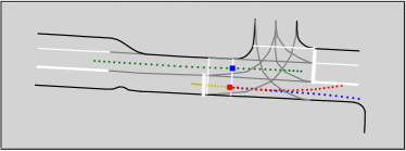
(a) CILF-MFP

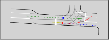
(b) Vanilla-MFP

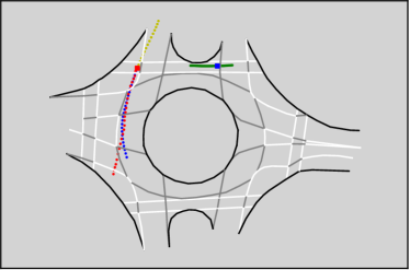
(c) CILF-MFP

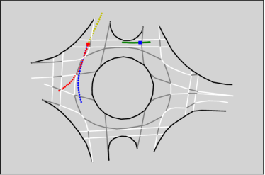
(d) Vanilla-MFP

Figure 3: Contrastive experiments between CILF-MFP and Vanilla-MFP on two target domains. (a) and (b) demonstrate the contrastive experiment on subset-3 (intersection) of INTERACTION, (c) and (d) demonstrate the contrastive experiment on subset-4 (roundabout) of INTERACTION.

6 Conclusion

To improve the generalization ability of vehicle trajectory prediction models, we first analyze the causal structure of OOD generalization and propose OOD-CG, which highlights the limitations of conventional correlation-based learning framework. Then we propose CILF to employ only causal features for prediction by three steps: (a) extracting IC by invariant risk minimization, (b) extracting V by domain contrastive learning, and (c) separating VC and VN by domain adversarial learning. Quantitative and qualitative experiments on several mainstream datasets prove the effectiveness of our model.

References

- [1] Alahi, A., Goel, K., Ramanathan, V., Robicquet, A., Fei-Fei, L., Savarese, S.: Social lstm: Human trajectory prediction in crowded spaces. In: Proceedings of the IEEE conference on computer vision and pattern recognition. pp. 961–971 (2016)
- [2] Arjovsky, M., Bottou, L., Gulrajani, I., Lopez-Paz, D.: Invariant risk minimization. arXiv preprint arXiv:1907.02893 (2019)
- [3] Bagi, S.S.G., Gharaee, Z., Schulte, O., Crowley, M.: Generative causal representation learning for out-of-distribution motion forecasting. arXiv preprint arXiv:2302.08635 (2023)
- [4] Chen, G., Li, J., Lu, J., Zhou, J.: Human trajectory prediction via counterfactual analysis. In: Proceedings of the IEEE/CVF International Conference on Computer Vision. pp. 9824–9833 (2021)
- [5] Deo, N., Trivedi, M.M.: Convolutional social pooling for vehicle trajectory prediction. In: Proceedings of the IEEE conference on computer vision and pattern recognition workshops. pp. 1468–1476 (2018)
- [6] Ganin, Y., Ustinova, E., Ajakan, H., Germain, P., Larochelle, H., Laviolette, F., Marchand, M., Lempitsky, V.: Domain-adversarial training of neural networks. The journal of machine learning research 17(1), 2096–2030 (2016)
- [7] Glymour, M., Pearl, J., Jewell, N.P.: Causal inference in statistics: A primer. John Wiley & Sons (2016)
- [8] Gretton, A., Borgwardt, K.M., Rasch, M.J., Schölkopf, B., Smola, A.: A kernel two-sample test. The Journal of Machine Learning Research 13(1), 723–773 (2012)
- [9] Jang, E., Gu, S., Poole, B.: Categorical reparameterization with gumbel-softmax. arXiv preprint arXiv:1611.01144 (2016)
- [10] Khosla, P., Teterwak, P., Wang, C., Sarna, A., Tian, Y., Isola, P., Maschinot, A., Liu, C., Krishnan, D.: Supervised contrastive learning. Advances in neural information processing systems 33, 18661–18673 (2020)
- [11] Lee, N., Choi, W., Vernaza, P., Choy, C.B., Torr, P.H., Chandraker, M.: Desire: Distant future prediction in dynamic scenes with interacting agents. In: Proceedings of the IEEE conference on computer vision and pattern recognition. pp. 336–345 (2017)
- [12] Lefèvre, S., Vasquez, D., Laugier, C.: A survey on motion prediction and risk assessment for intelligent vehicles. ROBOMECH journal 1(1), 1–14 (2014)
- [13] Li, S., Xue, Q., Shi, D., Li, X., Zhang, W.: Recursive least squares based refinement network for vehicle trajectory prediction. Electronics 11(12), 1859 (2022)
- [14] Liu, Y., Cadei, R., Schweizer, J., Bahmani, S., Alahi, A.: Towards robust and adaptive motion forecasting: A causal representation perspective. In: Proceedings of the IEEE/CVF Conference on Computer Vision and Pattern Recognition. pp. 17081–17092 (2022)
- [15] Long, M., Zhu, H., Wang, J., Jordan, M.I.: Deep transfer learning with joint adaptation networks. In: International conference on machine learning. pp. 2208–2217. PMLR (2017)
- [16] Lv, F., Liang, J., Li, S., Zang, B., Liu, C.H., Wang, Z., Liu, D.: Causality inspired representation learning for domain generalization. In: Proceedings of the IEEE/CVF Conference on Computer Vision and Pattern Recognition. pp. 8046–8056 (2022)
- [17] Motiian, S., Piccirilli, M., Adjeroh, D.A., Doretto, G.: Unified deep supervised domain adaptation and generalization. In: Proceedings of the IEEE international conference on computer vision. pp. 5715–5725 (2017)
- [18] Nguyen, T., Do, K., Nguyen, D.T., Duong, B., Nguyen, T.: Front-door adjustment via style transfer for out-of-distribution generalisation. arXiv preprint arXiv:2212.03063 (2022)
- [19] Paden, B., Čáp, M., Yong, S.Z., Yershov, D., Frazzoli, E.: A survey of motion planning and control techniques for self-driving urban vehicles. IEEE Transactions on intelligent vehicles 1(1), 33–55 (2016)
- [20] Pearl, J.: Causality. Cambridge university press (2009)
- [21] Peters, J., Janzing, D., Schölkopf, B.: Elements of causal inference: foundations and learning algorithms. The MIT Press (2017)
- [22] Punzo, V., Borzacchiello, M.T., Ciuffo, B.: On the assessment of vehicle trajectory data accuracy and application to the next generation simulation (ngsim) program data. Transportation Research Part C: Emerging Technologies 19(6), 1243–1262 (2011)
- [23] Reichenbach, H.: The Direction of Time. Mineola, N.Y.: Dover Publications (1956)
- [24] Schölkopf, B., Janzing, D., Peters, J., Sgouritsa, E., Zhang, K., Mooij, J.: On causal and anticausal learning. arXiv preprint arXiv:1206.6471 (2012)
- [25] Schölkopf, B., Locatello, F., Bauer, S., Ke, N.R., Kalchbrenner, N., Goyal, A., Bengio, Y.: Toward causal representation learning. Proceedings of the IEEE 109(5), 612–634 (2021)
- [26] Sutskever, I., Vinyals, O., Le, Q.V.: Sequence to sequence learning with neural networks. Advances in neural information processing systems 27 (2014)
- [27] Tang, C., Salakhutdinov, R.R.: Multiple futures prediction. Advances in neural information processing systems 32 (2019)
- [28] Tzeng, E., Hoffman, J., Saenko, K., Darrell, T.: Adversarial discriminative domain adaptation. In: Proceedings of the IEEE conference on computer vision and pattern recognition. pp. 7167–7176 (2017)
- [29] Yoon, C., Hamarneh, G., Garbi, R.: Generalizable feature learning in the presence of data bias and domain class imbalance with application to skin lesion classification. In: Medical Image Computing and Computer Assisted Intervention–MICCAI 2019: 22nd International Conference, Shenzhen, China, October 13–17, 2019, Proceedings, Part IV 22. pp. 365–373. Springer (2019)
- [30] Zhan, W., Sun, L., Wang, D., Shi, H., Clausse, A., Naumann, M., Kummerle, J., Konigshof, H., Stiller, C., de La Fortelle, A., et al.: Interaction dataset: An international, adversarial and cooperative motion dataset in interactive driving scenarios with semantic maps. arXiv preprint arXiv:1910.03088 (2019)
- [31] Zhang, W., Ouyang, W., Li, W., Xu, D.: Collaborative and adversarial network for unsupervised domain adaptation. In: Proceedings of the IEEE conference on computer vision and pattern recognition. pp. 3801–3809 (2018)
- [32] Zhou, K., Liu, Z., Qiao, Y., Xiang, T., Loy, C.C.: Domain generalization: A survey. IEEE Transactions on Pattern Analysis and Machine Intelligence (2022)