On the gap probability of the tacnode process

Abstract

The tacnode process is a universal determinantal point process arising from non-intersecting particle systems and tiling problems. It is the aim of this work to explore the integrable structure and large gap asymptotics for the gap probability of the thinned/unthinned tacnode process over $(-s,s)$. We establish an integral representation of the gap probability in terms of the Hamiltonian associated with a system of differential equations. With the aids of some remarkable differential identities for the Hamiltonian, we also compute large gap asymptotics, up to and including the constant term in the thinned case. As direct applications, we obtain expectation, variance and a central limit theorem for the associated counting function.

1 Introduction

Since the seminal work of Dyson on the Brownian motion model for eigenvalues of Gaussian unitary ensemble [41], there has been significant interest in ensembles of non-intersecting paths. Among them, non-intersecting Brownian motion models and their variants have been most studied over the last few decades. Besides their intimate connections with a variety of physical, combinatorial and probabilistic models [44, 46, 49, 58, 59, 61, 62, 77], the long-standing interest in non-intersecting Brownian motions is due in large part to the fact that the scaling limits lead to universal determinantal point processes related to random matrix theory and the KPZ universality class.

In a typical case, we consider $n$ 1D non-intersecting Brownian motion paths with several prescribed starting and ending points. For any fixed time, the positions of these paths form a determinantal point process. As the number of paths tends to infinity, these paths will, after proper scalings, fill out a region in the time-space plane with a deterministic limit shape. It comes out that the local statistics of this model is governed by sine process in the interior of the shape [10, 14, 29, 60, 67, 68], by the Airy process at the edge of the limit shape [10, 14, 29, 51, 69], and by the Pearcey process at the cusp [7, 9, 14, 21, 22, 75]; see also [2, 3, 28, 71] for relevant studies.

In this paper, we focus on a critical process arising from non-intersecting Brownian motions and random walk paths called tacnode process. This process appears in the case of critical separation, that is, two groups of Brownian motions are asymptotically distributed in two ellipses in the time-space plane which are tangent to each other (critical separation) and create a tacnode point; see Figure 1 for an illustration. The tacnode process then describes local correlations of the paths around this point. As a determinantal process, the tacnode process is characterized by a two-variable correlation function $K_{\mathrm{tac}}(x,y)$ called the tacnode kernel and the kernel also depends on some extra parameters relevant to the scalings. The tacnode process was studied by different groups of authors using different techniques. Adler, Ferrari and van Moerbeke [4] resolved the tacnode problem for non-intersecting random walks on $\mathbb{Z}$ (discrete space and continuous time). Johansson [57] gave an integral representation of the tacnode kernel in the continuous time-space setting. Ferrari and Vető [43] extended the results of Johansson to the non-symmetric case when the two touching groups of Brownian motions may have different sizes. In all these studies, the tacnode kernel is expressed using resolvents and Fredholm determinants of the Airy integral operator. An alternative expression of the tacnode kernel is given by Delvaux, Kuijlaars and the second author [38] with the aid of a new $4\times 4$ matrix-valued Riemann-Hilbert (RH) problem. This RH problem has a remarkable connection with the Hastings-McLeod solution [50] of the homogeneous Painlevé II equation

$$q^{\prime\prime}(x)=2q(x)^{3}+xq(x).$$ (1.1)

A natural question is then to ask whether all these formulas for the tacnode kernel lead to the same process, although it is generally believed to be the case. The equivalence of the RH formulation of the tacnode kernel in [38] and the Airy resolvent type formula of Johansson [57] was later established in [37], while the two different Airy type formulas obtained in [4] and [57] was proved to be equivalent in [6] based on an indirect way.

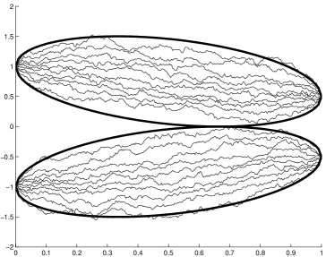
Figure 1: Simulation picture of 20 rescaled non-intersecting Brownian motion paths in the case of critical separation.

Similar to the canonical Sine, Airy and Pearcey point processes, the tacnode process (or its variant) represents a universality class in a wide range of problems in probability and mathematical physics. Some concrete examples include non-intersecting Brownian motions on the unit circle [23, 70] and various random tilling models [5, 6, 8], among others.

We intend to investigate the gap probability of the tacnode process – a basic object in the theory of point processes. More precisely, let $\mathcal{K}_{\mathrm{tac}}$ be the integral operator acting on $L^{2}\left(-s,s\right)$, $s\geq 0$, with the tacnode kernel $K_{\mathrm{tac}}$ and consider the associated Fredholm determinant $D(s;\gamma):=\det\left(I-\gamma\mathcal{K}_{\mathrm{tac}}\right)$, where $0<\gamma\leq 1$ is a real parameter. The determinantal structure implies that $D(s;1)$ can be interpreted as the probability of finding no particles (a.k.a. the gap probability) on the interval $(-s,s)$ for the tacnode process, while the deformed determinant $D(s;\gamma)$, $0<\gamma<1$, gives us gap probability for the thinned tacnode process. The thinned process is related to the original one by removing each particle independently with probability $1-\gamma$ (cf. [52]), and according to a general result in [25], the information of $D(s;\gamma)$ is essential in establishing global rigidity result for the tacnode process.

Beyond the fundamental meaning of $D(s;\gamma)$ just described, our study is also highly motivated by rich structures of Fredholm determinants for canonical universality classes. For instance, the celebrated Tracy-Widom distribution established in [76] shows that the Airy-kernel determinant admits an integral representation via the Hastings-McLeod solution of (1.1), which also leads to a conjecture of the large gap asymptotic formula. This conjecture was rigorously proved in [11, 33, 34] using different approaches. The same integral formula holds for the deformed Airy-kernel determinant but in terms of the Ablowitz-Segur solution [1, 73] of (1.1) instead; cf. [17, 19]. Large gap asymptotics in this case, however, exhibits a significantly different behavior from the undeformed case, as conjectured in [16] and lately proved in [19, 20]. Analogous results can be found in [12, 34, 40, 42, 55, 64, 78] for the sine-kernel determinant, and in [21, 26, 30, 31] for the Pearcey-kernel determinants.

Due to the highly transcendental form of the tacnode kernel, it remains an intriguing open problem to explore the integrable structure and large $s$ asymptotics of $D(s;\gamma)$; see however [13, 47, 48] for the transitions between the tacnode process and the Airy, Pearcey processes. It is the aim of this paper to resolve these problems and our results are stated in the next section.

Notations

Throughout this paper, the following notations are frequently used.

• If $A$ is a matrix, then $(A)_{ij}$ stands for its $(i,j)$-th entry and $A^{\mathsf{T}}$ stands for its transpose. An unimportant entry of $A$ is denoted by $\ast$. We use $I$ to denote an identity matrix, and the size might differ in different contexts. To emphasize a $k\times k$ identity matrix, we also use the notation $I_{k}$.

• It is notationally convenient to denote by $E_{j,k}$ the $4\times 4$ elementary matrix whose entries are all $0$, except for the $(j,k)$-entry, which is $1$, that is,

  $$E_{j,k}=\left(\delta_{l,j}\delta_{k,m}\right)_{l,m=1}^{4},$$ (1.2)

  where $\delta_{j,k}$ is the Kronecker delta.

• We denote by $D(z_{0},r)$ the open disc centred at $z_{0}$ with radius $r>0$, i.e.,

  $$D(z_{0},r):=\{z\in\mathbb{C}\mid|z-z_{0}|<r\},$$ (1.3)

  and by $\partial D(z_{0},r)$ its boundary. The orientation of $\partial D(z_{0},r)$ is taken in a clockwise manner.

• As usual, the three Pauli matrices $\{\sigma_{j}\}_{j=1}^{3}$ are defined by

  $$\sigma_{1}=\begin{pmatrix}0&1\\ 1&0\end{pmatrix},\qquad\sigma_{2}=\begin{pmatrix}0&-\mathrm{i}\\ \mathrm{i}&0\end{pmatrix},\qquad\sigma_{3}=\begin{pmatrix}1&0\\ 0&-1\end{pmatrix}.$$ (1.4)

• From time to time, we will encounter some functions that depend on the real parameters $r_{1},r_{2},s_{1},s_{2}$ and $\tau$. If $x(\cdot;r_{1},r_{2},s_{1},s_{2},\tau)$ is such a function, we set

  $$\widetilde{x}(\cdot;r_{1},r_{2},s_{1},s_{2},\tau) =x(\cdot;r_{2},r_{1},s_{2},s_{1},\tau),$$ (1.5)

  $$\dot{x}(\cdot;r_{1},r_{2},s_{1},s_{2},\tau) =x(\cdot;r_{1},r_{2},s_{1},s_{2},-\tau).$$ (1.6)

  Clearly, one has $x=\widetilde{x}$ if $r_{1}=r_{2}$ and $s_{1}=s_{2}$, and $x=\dot{x}$ if $\tau=0$.

2 Main results

2.1 Definition of the tacnode kernel

As mentioned previously, there exist several equivalent formulas of the tacnode kernel. We use the one that is defined through the following $4\times 4$ tacnode RH problem [38, 39].

RH problem 2.1.

• $M(z)=M(z;r_{1},r_{2},s_{1},s_{2},\tau)$ is analytic for $z\in\mathbb{C}\setminus\Gamma_{M}$, where the parameters $r_{1},r_{2},s_{1},s_{2},\tau$ are real with $r_{i}>0$, $i=1,2$, and

  $$\Gamma_{M}:=\cup_{k=0}^{5}\Gamma_{k}\cup\{0\}$$ (2.1)

  with

  $$\Gamma_{0}=(0,+\infty), \Gamma_{1}=e^{\varphi\mathrm{i}}(0,+\infty), \Gamma_{2}=e^{-\varphi\mathrm{i}}(-\infty,0),$$ (2.2)

  $$\Gamma_{3}=(-\infty,0), \Gamma_{4}=e^{\varphi\mathrm{i}}(-\infty,0), \Gamma_{5}=e^{-\varphi\mathrm{i}}(0,+\infty),\quad 0<\varphi<\frac{\pi}{3};$$

  see Figure 2 for an illustration of the contour $\Gamma_{M}$.

• For $z\in\Gamma_{k}$, $k=0,1,\ldots,5$, the limiting values

  $$M_{+}(z)=\lim_{\begin{subarray}{c}\zeta\to z\\ \zeta\textrm{ on $+$-side of }\Gamma_{k}\end{subarray}}M(\zeta),\qquad M_{-}(z)=\lim_{\begin{subarray}{c}\zeta\to z\\ \zeta\textrm{ on $-$-side of }\Gamma_{k}\end{subarray}}M(\zeta),$$

  exist, where the $+$-side and $-$-side of $\Gamma_{k}$ are the sides which lie on the left and right of $\Gamma_{k}$, respectively, when traversing $\Gamma_{k}$ according to its orientation. These limiting values satisfy the jump relation

  $$M_{+}(z)=M_{-}(z)J_{k}(z),\qquad k=0,\ldots,5,$$ (2.3)

  where the jump matrix $J_{k}(z)$ for each ray $\Gamma_{k}$ is shown in Figure 2.

• As $z\to\infty$ with $z\in\mathbb{C}\setminus\Gamma_{M}$, we have

  $$M(z) =\left(I+\frac{M^{(1)}}{z}+\mathcal{O}(z^{-2})\right)\operatorname{diag}\left((-z)^{-\frac{1}{4}},z^{-\frac{1}{4}},(-z)^{\frac{1}{4}},z^{\frac{1}{4}}\right)$$

  $$\quad\times A\operatorname{diag}\left(e^{-\theta_{1}(z)+\tau z},e^{-\theta_{2}(z)-\tau z},e^{\theta_{1}(z)+\tau z},e^{\theta_{2}(z)-\tau z}\right),$$ (2.4)

  where the matrix $M^{(1)}$ is independent of $z$ but depends on the parameters,

  $$A :=\frac{1}{\sqrt{2}}\begin{pmatrix}1&0&-\mathrm{i}&0\\ 0&1&0&\mathrm{i}\\ -\mathrm{i}&0&1&0\\ 0&\mathrm{i}&0&1\end{pmatrix},$$ (2.5)

  $$\theta_{1}(z) =\frac{2}{3}r_{1}(-z)^{\frac{3}{2}}+2s_{1}(-z)^{\frac{1}{2}},\qquad z\in\mathbb{C}\setminus[0,\infty),$$ (2.6)

  $$\theta_{2}(z) =\frac{2}{3}r_{2}z^{\frac{3}{2}}+2s_{2}z^{\frac{1}{2}},\qquad z\in\mathbb{C}\setminus(-\infty,0].$$ (2.7)

• $M(z)$ is bounded near $z=0$.

Figure 2: The jump contours $\Gamma_{k}$ and the corresponding jump matrices $J_{k}$, $k=0,\ldots,5$, in the RH problem for $M$.

The jump contour of the original tacnode RH problem consists of ten rays emanating from the origin. Here, as in [65], we reduce the number of rays to six by combining the two jumps in each of the open quadrants. The existence of a unique solution to the tacnode RH problem was proved for $\tau=0$ by Delvaux, Kuijlaars and the second author [38], for the symmetric case $r_{1}=r_{2}=1$, $s_{1}=s_{2}$ with general $\tau$ by Duits and Geudens [39], for the non-symmetric case by Delvaux [37].

Remark 2.2.

The RH problem for $X$ is related to the Hastings-McLeod solution of the Painlevé II equation (1.1) through the “residue” term $M^{(1)}$ in ((c)). More precisely, the Hastings-McLeod solution and associated Hamiltonian appear in the top right $2\times 2$ block of the matrix $M^{(1)}$; see [37, 38, 39]. Note that $M$ satisfies the following symmetric relations (see [37, 38]):

$$M(-z;r_{1},r_{2},s_{1},s_{2},\tau) =\begin{pmatrix}J&0\\ 0&-J\end{pmatrix}\widetilde{M}(z)\begin{pmatrix}J&0\\ 0&-J\end{pmatrix},$$ (2.8)

$$M(z;r_{1},r_{2},s_{1},s_{2},\tau)^{-\mathsf{T}} =\begin{pmatrix}0&-I_{2}\\ I_{2}&0\end{pmatrix}\dot{M}(z)\begin{pmatrix}0&I_{2}\\ -I_{2}&0\end{pmatrix},$$ (2.9)

where

$$J=\begin{pmatrix}0&1\\ 1&0\end{pmatrix},$$ (2.10)

$\widetilde{M}$ and $\dot{M}$ are defined through (1.5) and (1.6). It is then readily seen that $M^{(1)}=M^{(1)}(r_{1},r_{2},s_{1},s_{2},\tau)$ satisfies the symmetric relations

$$M^{(1)} =-\begin{pmatrix}J&0\\ 0&-J\end{pmatrix}\widetilde{M}^{(1)}\begin{pmatrix}J&0\\ 0&-J\end{pmatrix},$$ (2.11)

$$(M^{(1)})^{\mathsf{T}} =-\begin{pmatrix}0&-I_{2}\\ I_{2}&0\end{pmatrix}\dot{M}^{(1)}\begin{pmatrix}0&I_{2}\\ -I_{2}&0\end{pmatrix}.$$ (2.12)

As a consequence, we have

$$M^{(1)}_{11} =-\widetilde{M}^{(1)}_{22}=-\dot{M}^{(1)}_{33}=\dot{\widetilde{M}}^{(1)}_{44},$$ (2.13)

$$M^{(1)}_{13} =\widetilde{M}^{(1)}_{24}=\dot{M}^{(1)}_{13},$$ (2.14)

$$M^{(1)}_{23} =\widetilde{M}^{(1)}_{14}=\dot{M}^{(1)}_{14}.$$ (2.15)

Let $\widehat{M}$ be the analytic continuation of the restriction of $M$ in the sector bounded by the rays $\Gamma_{1}$ and $\Gamma_{2}$ to the whole complex plane. The tacnode kernel $K_{\mathrm{tac}}(x,y):=K_{\mathrm{tac}}(x,y;r_{1},r_{2},s_{1},s_{2},\tau)$ is then given in terms of $\widehat{M}$ by [38, Definition 2.6]

$$K_{\mathrm{tac}}(x,y)=\frac{1}{2\pi\mathrm{i}(x-y)}\begin{pmatrix}0&0&1&1\end{pmatrix}\widehat{M}(y)^{-1}\widehat{M}(x)\begin{pmatrix}1\\ 1\\ 0\\ 0\end{pmatrix}.$$ (2.16)

Define

$$F(s;\gamma)=F(s;\gamma,r_{1},r_{2},s_{1},s_{2},\tau):=\ln(D(s;\gamma))=\ln\det\left(I-\gamma\mathcal{K}_{\mathrm{tac}}\right),\quad 0<\gamma\leq 1.$$ (2.17)

Our first result is an integral representation of $F$ as stated in what follows.

2.2 An integral representation of $F$

The integral representation of $F$ involves the Hamiltonian of a system of coupled differential equations. These differential equations are given as follows:

$$\left\{\begin{aligned} p_{1}^{\prime}(s)&=-\mathrm{i}r_{1}sp_{3}(s)-p_{1}(s)p_{5}(s)-\mathrm{i}r_{1}p_{2}(s)\widetilde{q}_{6}(s)-\mathrm{i}r_{1}p_{3}(s)q_{5}(s)+p_{4}(s)p_{6}(s)-\tau p_{1}(s)\\ &\quad+\mathrm{i}s_{1}p_{3}(s)-\frac{\widetilde{p}_{2}(s)}{s}(p_{1}(s)\widetilde{q}_{2}(s)+p_{2}(s)\widetilde{q}_{1}(s)-p_{3}(s)\widetilde{q}_{4}(s)-p_{4}(s)\widetilde{q}_{3}(s)),\\ p_{2}^{\prime}(s)&=\mathrm{i}r_{2}sp_{4}(s)+\mathrm{i}r_{2}p_{1}(s)q_{6}(s)+p_{2}(s)\widetilde{p}_{5}(s)+p_{3}(s)\widetilde{p}_{6}(s)-\mathrm{i}r_{2}p_{4}(s)\widetilde{q}_{5}(s)+\tau p_{2}(s)\\ &\quad+\mathrm{i}s_{2}p_{4}(s)-\frac{\widetilde{p}_{1}(s)}{s}(p_{1}(s)\widetilde{q}_{2}(s)+p_{2}(s)\widetilde{q}_{1}(s)-p_{3}(s)\widetilde{q}_{4}(s)-p_{4}(s)\widetilde{q}_{3}(s)),\\ p_{3}^{\prime}(s)&=-\mathrm{i}r_{1}p_{1}(s)+p_{3}(s)p_{5}(s)-\mathrm{i}r_{2}p_{4}(s)\widetilde{q}_{6}(s)-\tau p_{3}(s)\\ &\quad+\frac{\widetilde{p}_{4}(s)}{s}(p_{1}(s)\widetilde{q}_{2}(s)+p_{2}(s)\widetilde{q}_{1}(s)-p_{3}(s)\widetilde{q}_{4}(s)-p_{4}(s)\widetilde{q}_{3}(s)),\\ p_{4}^{\prime}(s)&=-\mathrm{i}r_{2}p_{2}(s)+\mathrm{i}r_{1}p_{3}(s)q_{6}(s)-p_{4}(s)\widetilde{p}_{6}(s)+\tau p_{4}(s)\\ &\quad+\frac{\widetilde{p}_{3}(s)}{s}(p_{1}(s)\widetilde{q}_{2}(s)+p_{2}(s)\widetilde{q}_{1}(s)-p_{3}(s)\widetilde{q}_{4}(s)-p_{4}(s)\widetilde{q}_{3}(s)),\\ p_{5}^{\prime}(s)&=-\mathrm{i}r_{1}(p_{3}(s)q_{1}(s)+\widetilde{p}_{4}(s)\widetilde{q}_{2}(s)),\\ p_{6}^{\prime}(s)&=\mathrm{i}r_{1}(p_{3}(s)q_{4}(s)-\widetilde{p}_{4}(s)\widetilde{q}_{3}(s))+\mathrm{i}r_{2}(p_{1}(s)q_{2}(s)-\widetilde{p}_{2}(s)\widetilde{q}_{1}(s)),\\ q_{1}^{\prime}(s)&=p_{5}(s)q_{1}(s)-\mathrm{i}r_{2}q_{2}(s)q_{6}(s)+\mathrm{i}r_{1}q_{3}(s)+\tau q_{1}(s)\\ &\quad+\frac{\widetilde{q}_{2}(s)}{s}(\widetilde{p}_{2}(s)q_{1}(s)+\widetilde{p}_{1}(s)q_{2}(s)-\widetilde{p}_{4}(s)q_{3}(s)-\widetilde{p}_{3}(s)q_{4}(s)),\\ q_{2}^{\prime}(s)&=\mathrm{i}r_{1}q_{1}(s)\widetilde{q}_{6}(s)-\widetilde{p}_{5}(s)q_{2}(s)+\mathrm{i}r_{2}q_{4}(s)-\tau q_{2}(s)\\ &\quad+\frac{\widetilde{q}_{1}(s)}{s}(\widetilde{p}_{2}(s)q_{1}(s)+\widetilde{p}_{1}(s)q_{2}(s)-\widetilde{p}_{4}(s)q_{3}(s)-\widetilde{p}_{3}(s)q_{4}(s)),\\ q_{3}^{\prime}(s)&=\mathrm{i}r_{1}sq_{1}(s)+\mathrm{i}r_{1}q_{1}(s)q_{5}(s)-\widetilde{p}_{6}(s)q_{2}(s)-p_{5}(s)q_{3}(s)-\mathrm{i}r_{1}q_{4}(s)q_{6}(s)-\mathrm{i}s_{1}q_{1}(s)\\ &\quad+\tau q_{3}(s)-\frac{\widetilde{q}_{4}(s)}{s}(\widetilde{p}_{2}(s)q_{1}(s)+\widetilde{p}_{1}(s)q_{2}(s)-\widetilde{p}_{4}(s)q_{3}(s)-\widetilde{p}_{3}(s)q_{4}(s)),\\ q_{4}^{\prime}(s)&=-\mathrm{i}r_{2}sq_{2}(s)-p_{6}(s)q_{1}(s)+\mathrm{i}r_{2}q_{2}(s)\widetilde{q}_{5}(s)+\mathrm{i}r_{2}q_{3}(s)\widetilde{q}_{6}(s)+\widetilde{p}_{5}(s)q_{4}(s)-\mathrm{i}s_{2}q_{2}(s)\\ &\quad-\tau q_{4}(s)-\frac{\widetilde{q}_{3}(s)}{s}(\widetilde{p}_{2}(s)q_{1}(s)+\widetilde{p}_{1}(s)q_{2}(s)-\widetilde{p}_{4}(s)q_{3}(s)-\widetilde{p}_{3}(s)q_{4}(s)),\\ q_{5}^{\prime}(s)&=p_{1}(s)q_{1}(s)-p_{3}(s)q_{3}(s)-\widetilde{p}_{2}(s)\widetilde{q}_{2}(s)+\widetilde{p}_{4}(s)\widetilde{q}_{4}(s),\\ q_{6}^{\prime}(s)&=-p_{4}(s)q_{1}(s)-\widetilde{p}_{3}(s)\widetilde{q}_{2}(s),\end{aligned}\right.$$ (2.18)

where

$$p_{k}(s)=p_{k}(s;\gamma,r_{1},r_{2},s_{1},s_{2},\tau),\qquad q_{k}(s)=q_{k}(s;\gamma,r_{1},r_{2},s_{1},s_{2},\tau),\qquad k=1,\ldots,6,$$

are 12 unknown functions, $\widetilde{p}_{k}(s)$ and $\widetilde{q}_{k}(s)$ are related to $p_{k}(s)$ and $q_{k}(s)$ by swapping the parameters $r_{1}\leftrightarrow r_{2}$ and $s_{1}\leftrightarrow s_{2}$; see the definition (1.5). By introducing the matrix-valued functions

$$A_{0}(s)=\begin{pmatrix}p_{5}(s)+\tau&-\mathrm{i}r_{2}q_{6}(s)&\mathrm{i}r_{1}&0\\ \mathrm{i}r_{1}\widetilde{q}_{6}(s)&-\widetilde{p}_{5}(s)-\tau&0&\mathrm{i}r_{2}\\ \mathrm{i}r_{1}q_{5}(s)-\mathrm{i}s_{1}&-\widetilde{p}_{6}(s)&-p_{5}(s)+\tau&-\mathrm{i}r_{1}q_{6}(s)\\ -p_{6}(s)&\mathrm{i}r_{2}\widetilde{q}_{5}(s)-\mathrm{i}s_{2}&\mathrm{i}r_{2}\widetilde{q}_{6}(s)&\widetilde{p}_{5}(s)-\tau\end{pmatrix},$$ (2.19)

$$A_{1}(s)=\begin{pmatrix}q_{1}(s)\\ q_{2}(s)\\ q_{3}(s)\\ q_{4}(s)\end{pmatrix}\begin{pmatrix}p_{1}(s)&p_{2}(s)&p_{3}(s)&p_{4}(s)\end{pmatrix},$$ (2.20)

and

$$A_{2}(s)=\begin{pmatrix}\widetilde{q}_{2}(s)\\ \widetilde{q}_{1}(s)\\ -\widetilde{q}_{4}(s)\\ -\widetilde{q}_{3}(s)\end{pmatrix}\begin{pmatrix}\widetilde{p}_{2}(s)&\widetilde{p}_{1}(s)&-\widetilde{p}_{4}(s)&-\widetilde{p}_{3}(s)\end{pmatrix},$$ (2.21)

one can check

$$H(s)=H(s;\gamma,r_{1},r_{2},s_{1},s_{2},\tau)$$

$$:=\begin{pmatrix}p_{1}(s)&p_{2}(s)&p_{3}(s)&p_{4}(s)\end{pmatrix}\left(\mathrm{i}(r_{1}E_{3,1}-r_{2}E_{4,2})s+A_{0}(s)+\frac{A_{2}(s)}{2s}\right)\begin{pmatrix}q_{1}(s)\\ q_{2}(s)\\ q_{3}(s)\\ q_{4}(s)\end{pmatrix}$$

$$\quad+\begin{pmatrix}\widetilde{p}_{2}(s)&\widetilde{p}_{1}(s)&-\widetilde{p}_{4}(s)&-\widetilde{p}_{3}(s)\end{pmatrix}\left(\mathrm{i}(r_{1}E_{3,1}-r_{2}E_{4,2})s-A_{0}(s)+\frac{A_{1}(s)}{2s}\right)\begin{pmatrix}\widetilde{q}_{2}(s)\\ \widetilde{q}_{1}(s)\\ -\widetilde{q}_{4}(s)\\ -\widetilde{q}_{3}(s)\end{pmatrix},$$ (2.22)

with $E_{i,j}$, $i,j=1,\ldots,4$, being the matrices defined in (1.2), is the Hamiltonian for the above system of differential equations, under the extra condition

$$\sum_{k=1}^{4}p_{k}(s)q_{k}(s)=0.$$ (2.23)

That is, we have

$$q_{k}^{\prime}(s)=\frac{\partial H}{\partial p_{k}},\qquad p_{k}^{\prime}(s)=-\frac{\partial H}{\partial q_{k}},\qquad k=1,...,6.$$ (2.24)

Theorem 2.3.

For $\gamma\in[0,1]$, with the function $F(s;\gamma)$ defined in (2.17), we have,

$$F(s;\gamma)=\int_{0}^{s}H(t;\gamma)\,\mathrm{d}t,\qquad s\in(0,\infty),$$ (2.25)

where $H$ is the Hamiltonian (2.2) associated with a family of special solutions to the system of differential equations (2.18). Moreover, $H(s)$ satisfies the following asymptotic behaviors: as $s\to 0^{+}$,

$$H(s)=\mathcal{O}(1),$$ (2.26)

and as $s\to+\infty$,

$$H(s)=\begin{cases}-\frac{r_{1}^{2}+r_{2}^{2}}{4}s^{2}+(r_{1}s_{1}+r_{2}s_{2})s-s_{1}^{2}-s_{2}^{2}-\frac{1}{4s}+\mathcal{O}(s^{-2}),&\qquad\gamma=1,\\ 2\mathrm{i}\beta(r_{1}+r_{2})s^{\frac{1}{2}}-2\mathrm{i}\beta(s_{1}+s_{2})s^{-\frac{1}{2}}\\ ~{}-(3\beta^{2}+\frac{\mathrm{i}\beta}{2}\cos{(2\vartheta(s))}+\frac{\mathrm{i}\beta}{2}\cos{(2\widetilde{\vartheta}(s))})s^{-1}+\mathcal{O}(s^{-\frac{3}{2}}),&\qquad 0\leq\gamma<1,\end{cases}$$ (2.27)

where

$$\beta:=\frac{1}{2\pi\mathrm{i}}\ln(1-\gamma),\qquad\gamma\in[0,1),$$ (2.28)

and

$$\vartheta(s) =\vartheta(s;r_{1},s_{1})=\frac{2r_{1}}{3}s^{\frac{3}{2}}-2s_{1}s+\frac{3\mathrm{i}\beta}{2}\ln s+\mathrm{i}\beta\ln(8(r_{1}-\frac{s_{1}}{s}))+\arg\Gamma(1+\beta),$$ (2.29)

$$\widetilde{\vartheta}(s) =\vartheta(s;r_{2},s_{2}),$$ (2.30)

with $\Gamma$ being the Euler’s gamma function.

The local behavior of $H$ near the origin in (2.26) ensures the integral (2.25) is well-defined. For $0<\gamma<1$, we also derive asymptotics of the family of special solutions in Proposition 8.1 below, which plays an important role in asymptotic studies of $F$.

2.3 Large gap asymptotics and applications

A direct application of Theorem 2.3 is that we can obtain the first few terms in the asymptotic expansion of $F(s;\gamma)$ as $s\to+\infty$ except for the constant term by inserting (2.27) into (2.25). For $0<\gamma<1$, we are also able to determine the notoriously difficult constant term.

Theorem 2.4.

With the function $F(s;\gamma)$ defined in (2.17), we have, as $s\to+\infty$,

$$F(s;\gamma)=\begin{cases}-\frac{r_{1}^{2}+r_{2}^{2}}{12}s^{3}+\frac{r_{1}s_{1}+r_{2}s_{2}}{2}s^{2}-(s_{1}^{2}+s_{2}^{2})s-\frac{\ln{s}}{4}+C+\mathcal{O}(s^{-1}),&\gamma=1,\\ \frac{4\beta\mathrm{i}(r_{1}+r_{2})}{3}s^{\frac{3}{2}}-4\beta\mathrm{i}(s_{1}+s_{2})s^{\frac{1}{2}}-3\beta^{2}\ln{s}+2\ln{(G(1+\beta)G(1-\beta))}\\ ~{}-\beta^{2}\ln{(64r_{1}r_{2})}+\mathcal{O}(s^{-\frac{1}{2}}),&0\leq\gamma<1,\end{cases}$$ (2.31)

uniformly for $r_{i}>0,i=1,2$ and $s_{i}\in\mathbb{R},i=1,2$, where $C$ is an undetermined constant independent of $s$, $\beta$ is given in (2.28) and $G(z)$ is the Barnes G-function.

If $\gamma=0$, we have that $\beta=0$ and $G(1+\beta)=G(1)=1$. It is then straightforward to see $F(s;0)=\mathcal{O}(s^{-1/2})$, which matches the fact that $F(s;0)=0$. If $\gamma=1$, our result supports the so-called Forrester-Chen-Eriksen-Tracy conjecture [27, 45]. This conjecture claims that the probability $E(s)$ of emptiness over the interval $(x^{*}-s,x^{*}+s)$ behaves like $\exp(-Ks^{2\alpha+2})$ for large positive $s$ with $K$ being some constant, provided the density of state behaves as $|x-x^{*}|^{\alpha}$ as $x\to x^{*}$. Since the limiting mean density for the non-intersecting Brownian paths at the time of tangency consists of two touching semicircles, it follows that $\alpha=1/2$ for the tacnode process. Thus, one should have $F(s;1)=\mathcal{O}(s^{3})$, as confirmed in (2.31). Also, we cannot evaluate explicitly the constant $C$ therein with our method, which in general is a challenging task; cf. [63].

Our final result is about counting statistics of the tacnode process. To proceed, we denote by $N(s)$ the random variable that counts the number of points in the tacnode process falling into the interval $(-s,s)$, $s\geq 0$. It is well known that the following generating functionx

$$\mathbb{E}\left(e^{-2\pi\nu N(s)}\right)=\sum_{k=0}^{\infty}\mathbb{P}(N(s)=k)e^{-2\pi\nu k},\qquad\nu\geq 0,$$ (2.32)

is equal to the deformed Fredholm determinant $\det\left(I-(1-e^{-2\pi\nu})\mathcal{K}_{\mathrm{tac}}\right)$. This, together with Theorem 2.4, allows us to establish various asymptotic statistical properties of $N$; see also [24, 25, 26, 30, 74] for relevant results about the sine, Airy and Pearcey point determinantal processes.

Corollary 2.5.

As $s\to+\infty$, we have

$$\mathbb{E}(N(s)) =\mu(s)+\mathcal{O}\left(\frac{\ln s}{s^{1/2}}\right),$$ (2.33)

$$\operatorname{Var}(N(s)) =\sigma(s)^{2}+\frac{2+2\gamma_{E}+\ln(64r_{1}r_{2})}{2\pi^{2}}+\mathcal{O}\left(\frac{(\ln s)^{2}}{s^{1/2}}\right),$$ (2.34)

where $\gamma_{E}=-\Gamma^{\prime}(1)\approx 0.57721$ is Euler’s constant,

$$\mu(s)=\frac{2(r_{1}+r_{2})}{3\pi}s^{\frac{3}{2}}-\frac{2(s_{1}+s_{2})}{\pi}s^{\frac{1}{2}},\qquad\sigma(s)^{2}=\frac{3}{2\pi^{2}}\ln s.$$ (2.35)

Furthermore, the random variable $\frac{N(s)-\mu(s)}{\sqrt{\sigma(s)^{2}}}$ converges in distribution to the normal law $\mathcal{N}(0,1)$as $s\to+\infty$, and for any $\epsilon>0$, we have

$$\lim_{a\to\infty}\mathbb{P}\left(\sup_{s>a}\left|\frac{N(s)-\mu(s)}{\ln s}\right|\leq\frac{3\sqrt{2}}{2\pi}+\epsilon\right)=1.$$ (2.36)

The probabilistic bound (2.36) particularly implies that, for large positive $s$, the counting function of the tacnode process lies in the interval $(\mu(s)-(3\sqrt{2}/(2\pi)+\epsilon)\ln s,\mu(s)+(3\sqrt{2}/(2\pi)+\epsilon)\ln s)$ with high probability.

Organization of the rest of the paper

The rest of this paper is devoted to the proofs of our main results. The idea is to relate various derivatives of $F$ to a $4\times 4$ RH problem under the general framework [18, 34]. In Section 3, we connect $\,\mathrm{d}F/\,\mathrm{d}s$ to a $4\times 4$ RH problem for $X$ with constant jumps. We then derive a lax pair for $X$ in Section 4, and some useful differential identities for the Hamiltonian will also be included for later calculation. We perform a Deift-Zhou steepest descent analysis [35] on the RH problem for $X$ as $s\to+\infty$ in Sections 5 and 6 for the cases $\gamma=1$ and $0\leq\gamma<1$, respectively, and deal with the small positive $s$ case in Section 7. After computing the asymptotics of a family of special solutions to the system of differential equations (2.18) and (2.23) in Section 8, we finally present the proofs of our main results in Section 9.

3 Preliminaries

We intend to establish a relation between $\,\mathrm{d}F/\,\mathrm{d}s$ and an RH problem with constant jumps. To proceed, we note that

$$\frac{\,\mathrm{d}}{\,\mathrm{d}s}F(s;\gamma)=-\textrm{tr}\left((I-\gamma\mathcal{K}_{\mathrm{tac}})^{-1}\gamma\frac{\,\mathrm{d}}{\,\mathrm{d}s}\mathcal{K}_{\mathrm{tac}}\right)=-(R(s,s)+R(-s,-s)),$$ (3.1)

where $R(u,v)$ stands for the kernel of the resolvent operator.

By (2.16), one readily sees that

$$\gamma K_{\mathrm{tac}}(x,y)=\frac{\mathbf{f}(x)^{\mathsf{T}}\mathbf{h}(y)}{x-y},$$ (3.2)

where

$$\mathbf{f}(x)=\begin{pmatrix}f_{1}\\ f_{2}\\ f_{3}\\ f_{4}\end{pmatrix}:=\widehat{M}(x)\begin{pmatrix}1\\ 1\\ 0\\ 0\end{pmatrix},\qquad\mathbf{h}(y)=\begin{pmatrix}h_{1}\\ h_{2}\\ h_{3}\\ h_{4}\end{pmatrix}:=\frac{\gamma}{2\pi\mathrm{i}}\widehat{M}(y)^{-\mathsf{T}}\begin{pmatrix}0\\ 0\\ 1\\ 1\end{pmatrix}.$$ (3.3)

This integrable structure of kernel $K_{\mathrm{tac}}$ in the sense of Its et al. [53] implies that the resolvent kernel $R(u,v)$ is integrable as well; cf. [35, 53]. Indeed, by setting

$$\mathbf{F}(u)=\begin{pmatrix}F_{1}\\ F_{2}\\ F_{3}\\ F_{4}\end{pmatrix}:=\left(I-\gamma\mathcal{K}_{\mathrm{tac}}\right)^{-1}\mathbf{f},\qquad\mathbf{H}(v)=\begin{pmatrix}H_{1}\\ H_{2}\\ H_{3}\\ H_{4}\end{pmatrix}:=\left(I-\gamma\mathcal{K}_{\mathrm{tac}}\right)^{-1}\mathbf{h},$$ (3.4)

we have

$$R(u,v)=\frac{\mathbf{F}(u)^{\mathsf{T}}\mathbf{H}(v)}{u-v}.$$ (3.5)

Moreover, the functions $\mathbf{F}(u)$ and $\mathbf{H}(u)$ are closely related to the following RH problem.

RH problem 3.1.

1. $Y(z)$ is a $4\times 4$ matrix-valued function defined and analytic in $\mathbb{C}\setminus[-s,s]$, where the orientation is taken from the left to the right.

2. For $x\in(-s,s)$, we have

   $$Y_{+}(x)=Y_{-}(x)(I-2\pi\mathrm{i}\mathbf{f}(x)\mathbf{h}(x)^{\mathsf{T}}),$$ (3.6)

   where the functions $\mathbf{f}$ and $\mathbf{h}$ are defined in (3.3).

3. As $z\to\infty$, we have

   $$Y(z)=I+\frac{Y^{(1)}}{z}+\mathcal{O}(z^{-2}).$$ (3.7)

   where the function $Y^{(1)}$ is independent of $z$.

4. As $z\to\pm s$, we have $Y(z)=\mathcal{\mathcal{O}}(\ln(z\mp s))$.

By [35], it follows that

$$Y(z)=I-\int_{-s}^{s}\frac{\mathbf{F}(w)\mathbf{h}(w)^{\mathsf{T}}}{w-z}\,\mathrm{d}w$$ (3.8)

and

$$\mathbf{F}(z)=Y(z)\mathbf{f}(z),\qquad\mathbf{H}(z)=Y(z)^{-\mathsf{T}}\mathbf{h}(z).$$ (3.9)

We now make an undressing transformation to arrive at an RH problem that is related to $\,\mathrm{d}F/\,\mathrm{d}s$ with the aid of the RH problems for $M$ and $Y$. We start with definitions

$$\Gamma_{0}^{(s)}:=(s,+\infty), \Gamma_{1}^{(s)}:=s+e^{\varphi\mathrm{i}}(0,+\infty), \Gamma_{2}^{(s)}:=-s+e^{-\varphi\mathrm{i}}(-\infty,0),$$ (3.10)

$$\Gamma_{3}^{(s)}:=(-\infty,-s), \Gamma_{4}^{(s)}:=-s+e^{\varphi\mathrm{i}}(-\infty,0), \Gamma_{5}^{(s)}:=s+e^{-\varphi\mathrm{i}}(0,+\infty),\quad 0<\varphi<\frac{\pi}{3}.$$

Clearly, the rays $\Gamma_{k}^{(s)}$, $k=1,2,4,5$, and $\mathbb{R}$ divide the whole complex plane into 6 regions $\Omega_{j}^{(s)}$, $j=1,\ldots,6$; see Figure 3 for an illustration. The transformation is defined by

$$X(z)=X(z;s,\gamma,r_{1},r_{2},s_{1},s_{2},\tau)$$

$$=\begin{cases}Y(z)M(z),&\hbox{ $z\in\Omega_{1}^{(s)}\cup\Omega_{3}^{(s)}\cup\Omega_{4}^{(s)}\cup\Omega_{6}^{(s)}$,}\\ Y(z)\widehat{M}(z),&\hbox{ $z\in\Omega_{2}^{(s)}$,}\\ Y(z)\widehat{M}(z)\begin{pmatrix}1&0&-1&-1\\ 0&1&-1&-1\\ 0&0&1&0\\ 0&0&0&1\end{pmatrix},&\hbox{ $z\in\Omega_{5}^{(s)}$.}\end{cases}$$ (3.11)

On account of the RH problems 2.1 and 3.1 for $M$ and $Y$, it is straightforward to check that $X$ satisfies the following RH problem.

Figure 3: Regions $\Omega_{j}^{(s)}$, $j=1,\ldots,6$, and the contours $\Gamma_{k}^{(s)}$, $k=0,1,\ldots,5$, for the RH problem for $\Phi$.

RH problem 3.2.

1. $X(z)$ is defined and analytic in $\mathbb{C}\setminus\Gamma_{X}$, where

   $$\Gamma_{X}:=\cup^{5}_{j=0}\Gamma_{j}^{(s)}\cup[-s,s]$$ (3.12)

   with the rays $\Gamma_{j}^{(s)}$, $j=0,1,\ldots,5$, defined in (3.10) and (LABEL:def:Gammajs2); see Figure 3 for the orientations of $\Gamma_{X}$.

2. For $z\in\Gamma_{X}$, $X$ satisfies the jump condition

   $$X_{+}(z)=X_{-}(z)J_{X}(z),$$ (3.13)

   where

   $$J_{X}(z):=\left\{\begin{array}[]{ll}\begin{pmatrix}0&0&1&0\\ 0&1&0&0\\ -1&0&0&0\\ 0&0&0&1\end{pmatrix},&\qquad\hbox{$z\in\Gamma_{0}^{(s)}$,}\\ I-E_{2,1}+E_{3,1}+E_{3,4},&\qquad\hbox{$z\in\Gamma_{1}^{(s)}$,}\\ I-E_{1,2}+E_{4,2}+E_{4,3},&\qquad\hbox{$z\in\Gamma_{2}^{(s)}$,}\\ \begin{pmatrix}1&0&0&0\\ 0&0&0&1\\ 0&0&1&0\\ 0&-1&0&0\end{pmatrix},&\qquad\hbox{$z\in\Gamma_{3}^{(s)}$,}\\ I+E_{1,2}+E_{4,2}-E_{4,3},&\qquad\hbox{$z\in\Gamma_{4}^{(s)}$,}\\ I+E_{2,1}+E_{3,1}-E_{3,4},&\qquad\hbox{$z\in\Gamma_{5}^{(s)}$,}\\ \begin{pmatrix}1&0&1-\gamma&1-\gamma\\ 0&1&1-\gamma&1-\gamma\\ 0&0&1&0\\ 0&0&0&1\end{pmatrix},&\qquad\hbox{$z\in(-s,s)$.}\end{array}\right.$$ (3.14)

3. As $z\to\infty$ with $z\in\mathbb{C}\setminus\Gamma_{X}$, we have

   $$X(z) =\left(I+\frac{X^{(1)}}{z}+\mathcal{O}(z^{-2})\right)\operatorname{diag}\left((-z)^{-\frac{1}{4}},z^{-\frac{1}{4}},(-z)^{\frac{1}{4}},z^{\frac{1}{4}}\right)$$

   $$\quad\times A\operatorname{diag}\left(e^{-\theta_{1}(z)+\tau z},e^{-\theta_{2}(z)-\tau z},e^{\theta_{1}(z)+\tau z},e^{\theta_{2}(z)-\tau z}\right),$$ (3.15)

   where $A$, $\theta_{1}$ and $\theta_{2}$ are defined in (2.5)–(2.7), respectively and

   $$X^{(1)}=Y^{(1)}+M^{(1)}$$ (3.16)

   with $Y^{(1)}$ and $M^{(1)}$ given in (3.7) and ((c)).

4. As $z\to s$, we have

   $$X(z) =X_{R}(z)\begin{pmatrix}1&0&-\frac{\gamma}{2\pi\mathrm{i}}\ln(z-s)&-\frac{\gamma}{2\pi\mathrm{i}}\ln(z-s)\\ 0&1&-\frac{\gamma}{2\pi\mathrm{i}}\ln(z-s)&-\frac{\gamma}{2\pi\mathrm{i}}\ln(z-s)\\ 0&0&1&0\\ 0&0&0&1\end{pmatrix}$$

   $$\quad\times\begin{cases}I,&z\in\Omega_{2}^{(s)},\\ \begin{pmatrix}1&0&-1&-1\\ 0&1&-1&-1\\ 0&0&1&0\\ 0&0&0&1\end{pmatrix},&z\in\Omega_{5}^{(s)},\end{cases}$$ (3.17)

   where the principal branch is taken for $\ln(z-s)$, and $X_{R}(z)$ is analytic at $z=s$ satisfying

   $$X_{R}(z)=X_{R,0}(s)\left(I+X_{R,1}(s)(z-s)+\mathcal{O}((z-s)^{2})\right),\qquad z\to s,$$ (3.18)

   for some functions $X_{R,0}(s)$ and $X_{R,1}(s)$ depending on the parameters $r_{1}$,$r_{2}$,$s_{1}$,$s_{2}$,$\tau$ and $\gamma$.

5. As $z\to-s$, we have

   $$X(z) =X_{L}(z)\begin{pmatrix}1&0&-\frac{\gamma}{2\pi\mathrm{i}}\ln(-z-s)&-\frac{\gamma}{2\pi\mathrm{i}}\ln(-z-s)\\ 0&1&-\frac{\gamma}{2\pi\mathrm{i}}\ln(-z-s)&-\frac{\gamma}{2\pi\mathrm{i}}\ln(-z-s)\\ 0&0&1&0\\ 0&0&0&1\end{pmatrix}$$

   $$\quad\times\begin{cases}\begin{pmatrix}0&1&0&0\\ 1&0&0&0\\ 0&0&0&-1\\ 0&0&-1&0\end{pmatrix},&z\in\Omega_{2}^{(s)},\\ \begin{pmatrix}0&1&1&1\\ 1&0&1&1\\ 0&0&0&-1\\ 0&0&-1&0\end{pmatrix},&z\in\Omega_{5}^{(s)},\end{cases}$$ (3.19)

   where $\ln(-z-s)$ is analytic for $z\in\mathbb{C}\setminus[-s,+\infty)$ and $X_{L}(z)$ is analytic at $z=-s$ satisfying

   $$X_{L}(z)=X_{L,0}(s)\left(I+X_{L,1}(s)(z+s)+\mathcal{O}((z+s)^{2})\right),\qquad z\to-s,$$ (3.20)

   for some functions $X_{L,0}(s)$ and $X_{L,1}(s)$ depending on the parameters $r_{1}$,$r_{2}$,$s_{1}$,$s_{2}$,$\tau$ and $\gamma$.

Proposition 3.3.

The matrix-valued function $X(z)$ satisfies the following symmetric relations:

$$X(-z) =\begin{pmatrix}J&0\\ 0&-J\end{pmatrix}\widetilde{X}(z)\begin{pmatrix}J&0\\ 0&-J\end{pmatrix},$$ (3.21)

$$X(z)^{-\mathsf{T}} =\begin{pmatrix}0&-I_{2}\\ I_{2}&0\end{pmatrix}\dot{X}(z)\begin{pmatrix}0&I_{2}\\ -I_{2}&0\end{pmatrix},$$ (3.22)

where $J$ is given in (2.10), $\widetilde{X}$ and $\dot{X}$ are defined through (1.5) and (1.6). Moreover, the matrix $X^{(1)}=X^{(1)}(\gamma,r_{1},r_{2},s_{1},s_{2},\tau)$ in ((c)) satisfies

$$X^{(1)} =-\begin{pmatrix}J&0\\ 0&-J\end{pmatrix}\widetilde{X}^{(1)}\begin{pmatrix}J&0\\ 0&-J\end{pmatrix},$$ (3.23)

$$(X^{(1)})^{\mathsf{T}} =-\begin{pmatrix}0&-I_{2}\\ I_{2}&0\end{pmatrix}\dot{X}^{(1)}\begin{pmatrix}0&I_{2}\\ -I_{2}&0\end{pmatrix}.$$ (3.24)

Proof.

One can check that the left and right hand sides of (3.21) satisfy the same RH problem. Then (3.21) follows from the uniqueness of the solution to this RH problem. The same argument applies to (3.22). By substituting the asymptotic behavior of $X(z)$ in ((c)) into equations (3.21) and (3.22), the symmetric relations (3.23) and (3.24) follow from a straightforward calculation.

This finishes the proof of Proposition 3.3. ∎

The connection between the derivatives of $F$ and the RH problem for $X$ is revealed in the following proposition.

Proposition 3.4.

With $F$ defined in (2.17), we have

$$\frac{\,\mathrm{d}}{\,\mathrm{d}s}F(s;\gamma,r_{1},r_{2},s_{1},s_{2},\tau)=-\frac{\gamma}{2\pi\mathrm{i}}\left[\lim_{z\to s}\sum_{i=3}^{4}\sum_{j=1}^{2}\left(X(z)^{-1}X^{\prime}(z)\right)_{ij}+\lim_{z\to-s}\sum_{i=3}^{4}\sum_{j=1}^{2}\left(X(z)^{-1}X^{\prime}(z)\right)_{ij}\right],$$ (3.25)

where the limit is taken from $\Omega_{2}^{(s)}$ and

$$\frac{\partial}{\partial s_{1}}F(s;\gamma,r_{1},r_{2},s_{1},s_{2},\tau) =2\mathrm{i}\left(X^{(1)}_{13}-M^{(1)}_{13}\right),$$ (3.26)

$$\frac{\partial}{\partial s_{2}}F(s;\gamma,r_{1},r_{2},s_{1},s_{2},\tau) =2\mathrm{i}\left(\widetilde{X}^{(1)}_{13}-\widetilde{M}^{(1)}_{13}\right),$$ (3.27)

$$\frac{\partial}{\partial\tau}F(s;\gamma,r_{1},r_{2},s_{1},s_{2},\tau) =-X^{(1)}_{11}-\widetilde{X}^{(1)}_{11}+\dot{X}^{(1)}_{11}+\dot{\widetilde{X}}^{(1)}_{11}$$

$$\quad+M^{(1)}_{11}+\widetilde{M}^{(1)}_{11}-\dot{M}^{(1)}_{11}-\dot{\widetilde{M}}^{(1)}_{11},$$ (3.28)

where $X^{(1)}$ and $M^{(1)}$ are given in ((c)) and ((c)). Here, for a function $x=x(\cdot;r_{1},r_{2},s_{1},s_{2},\tau)$, we have $\dot{\widetilde{x}}=x(\cdot;r_{2},r_{1},s_{2},s_{1},-\tau))$; see the notations (1.5) and (1.6).

To prove Proposition 3.4, we need the following lemma.

Lemma 3.5.

Let $M$ be the unique solution to the tacnode RH problem 2.1, we have

$$\frac{\partial M}{\partial s_{1}} =-2\mathrm{i}\left(E_{1,3}+zE_{3,1}+\left[M^{(1)},E_{3,1}\right]\right)M,$$ (3.29)

$$\frac{\partial M}{\partial s_{2}} =-2\mathrm{i}\left(-E_{2,4}+zE_{4,2}+\left[M^{(1)},E_{4,2}\right]\right)M,$$ (3.30)

$$\frac{\partial M}{\partial\tau} =\left(\begin{pmatrix}z&0&0&0\\ 0&-z&0&0\\ 0&0&z&0\\ 0&0&0&-z\end{pmatrix}+\left[M^{(1)},\begin{pmatrix}1&0&0&0\\ 0&-1&0&0\\ 0&0&1&0\\ 0&0&0&-1\end{pmatrix}\right]\right)M,$$ (3.31)

where $[A,B]$ denotes the commutation of two matrices, i.e., $[A,B]=AB-BA$.

Proof.

Since the RH problem for $M$ has constant jumps, we obtain from the local behavior of $M$ near the origin that $(\partial M/\partial s_{1})M^{-1}$ is entire. As $z\to\infty$, we find from ((c)) that

$$\frac{\partial M}{\partial s_{1}}M^{-1} =\left(I+\frac{M^{(1)}}{z}+\mathcal{O}(z^{-2})\right)\operatorname{diag}\left((-z)^{-\frac{1}{4}},z^{-\frac{1}{4}},(-z)^{\frac{1}{4}},z^{\frac{1}{4}}\right)A\operatorname{diag}\left(-2(-z)^{\frac{1}{2}},0,2(-z)^{\frac{1}{2}},0\right)$$

$$\quad\times A^{-1}\operatorname{diag}\left((-z)^{\frac{1}{4}},z^{\frac{1}{4}},(-z)^{-\frac{1}{4}},z^{-\frac{1}{4}}\right)\left(I-\frac{M^{(1)}}{z}+\mathcal{O}(z^{-2})\right)+\mathcal{O}(z^{-1})$$

$$=-2\mathrm{i}\left(E_{1,3}+zE_{3,1}+\left[M^{(1)},E_{3,1}\right]\right)+\mathcal{O}(z^{-1})$$ (3.32)

Keeping only the polynomial terms in $z$, we obtain (3.29). A similar argument yields (3.30) and (3.31).

This finishes the proof of Lemma 3.5. ∎

Proof of Proposition 3.4.

For $z\in\Omega_{2}^{(s)}$, we see from (3.3), (3.9) and (3) that

$$\mathbf{F}(z)=Y(z)\mathbf{f}(z)=Y(z)\widehat{M}(z)\begin{pmatrix}1\\ 1\\ 0\\ 0\end{pmatrix}=X(z)\begin{pmatrix}1\\ 1\\ 0\\ 0\end{pmatrix}$$ (3.33)

and

$$\mathbf{H}(z) =Y(z)^{-\mathsf{T}}\mathbf{h}(z)=X(z)^{-\mathsf{T}}\widehat{M}(z)^{\mathsf{T}}\cdot\frac{\gamma}{2\pi\mathrm{i}}\widehat{M}(z)^{-\mathsf{T}}\begin{pmatrix}0\\ 0\\ 1\\ 1\end{pmatrix}=\frac{\gamma}{2\pi\mathrm{i}}X(z)^{-\mathsf{T}}\begin{pmatrix}0\\ 0\\ 1\\ 1\end{pmatrix}.$$ (3.34)

Combining the above formulas and (3.5), we obtain

$$R(z,z)=\frac{\gamma}{2\pi\mathrm{i}}\sum_{i=3}^{4}\sum_{j=1}^{2}\left(X(z)^{-1}X^{\prime}(z)\right)_{ij},\qquad z\in\Omega_{2}^{(s)}.$$ (3.35)

This, together with (3.1), gives us (3.25).

To show (3.26), we note from (3.3) and (3.29) that

$$\frac{\partial\mathbf{f}}{\partial s_{1}}(x)=-2\mathrm{i}\left(E_{1,3}+xE_{3,1}+\left[M^{(1)},E_{3,1}\right]\right)\mathbf{f}(x),$$ (3.36)

$$\frac{\partial\mathbf{h}}{\partial s_{1}}(y)=2\mathrm{i}\left(E_{1,3}+yE_{3,1}+\left[M^{(1)},E_{3,1}\right]\right)^{\mathsf{T}}\mathbf{h}(y).$$ (3.37)

The above equations, together with (3.2), imply that

$$\frac{\partial}{\partial s_{1}}\left(\gamma K_{\mathrm{tac}}(x,y)\right) =\frac{\frac{\partial\mathbf{f}^{\mathsf{T}}}{\partial s_{1}}(x)\mathbf{h}(y)+\mathbf{f}(x)^{\mathsf{T}}\frac{\partial\mathbf{h}}{\partial s_{1}}(y)}{x-y}$$

$$=-2\mathrm{i}\mathbf{f}(x)^{\mathsf{T}}E_{1,3}\mathbf{h}(y)=-2\mathrm{i}f_{1}(x)h_{3}(y).$$ (3.38)

Thus, it is readily seen from (2.17) and (3.4) that

$$\frac{\partial}{\partial s_{1}}F(s;\gamma,r_{1},r_{2},s_{1},s_{2},\tau) =\frac{\partial}{\partial s_{1}}\ln\det\left(I-\gamma\mathcal{K}_{\mathrm{tac}}\right)=-\operatorname{Tr}{\left((I-\gamma\mathcal{K}_{\mathrm{tac}})^{-1}\frac{\partial}{\partial s_{1}}\left(\gamma\mathcal{K}_{\mathrm{tac}}\right)\right)}$$

$$=2\mathrm{i}\int_{-s}^{s}F_{1}(v)h_{3}(v)\,\mathrm{d}v$$ (3.39)

On the other hand, from (3.7) and (3.8) we have

$$Y^{(1)}=\int_{-s}^{s}\mathbf{F}(v)\mathbf{h}(v)^{\mathsf{T}}\,\mathrm{d}v.$$ (3.40)

A combination of the above two equations gives us

$$\frac{\partial}{\partial s_{1}}F(s;\gamma,r_{1},r_{2},s_{1},s_{2},\tau)=2\mathrm{i}Y^{(1)}_{13}.$$ (3.41)

We thus obtain (3.26) by applying (3.16) to the above formula.

Through a similar calculation, we have

$$\frac{\partial}{\partial s_{2}}F(s;\gamma,r_{1},r_{2},s_{1},s_{2},\tau) =2\mathrm{i}Y^{(1)}_{24},$$ (3.42)

$$\frac{\partial}{\partial\tau}F(s;\gamma,r_{1},r_{2},s_{1},s_{2},\tau) =-Y^{(1)}_{11}+Y^{(1)}_{22}-Y^{(1)}_{33}+Y^{(1)}_{44}.$$ (3.43)

Substituting (3.16) into the above equations and using the symmetric relations (2.14), (2.13), (3.23) and (3.24), we arrive at (3.27) and (3.28).

This completes the proof of Proposition 3.4. ∎

4 Lax pair equations and differential identities for the Hamiltonian

In this section, we will derive a Lax pair for $X(z;s)$ from RH problem 3.2. Several useful differential identities for the associated Hamiltonian will also be presented for later use.

4.1 The Lax system for $X$

Proposition 4.1.

For the matrix-valued function $X(z)=X(z;s)$ defined in (3), we have

$$\frac{\partial}{\partial z}X(z;s)=L(z;s)X(z;s),\qquad\frac{\partial}{\partial s}X(z;s)=U(z;s)X(z;s),$$ (4.1)

where

$$L(z;s)=\mathrm{i}(r_{1}E_{3,1}-r_{2}E_{4,2})z+A_{0}(s)+\frac{A_{1}(s)}{z-s}+\frac{A_{2}(s)}{z+s},$$ (4.2)

and

$$U(z;s)=-\frac{A_{1}(s)}{z-s}+\frac{A_{2}(s)}{z+s}$$ (4.3)

with the functions $A_{k}(s)$, $k=0,1,2$, given in (2.19)–(2.21), respectively. Moreover, the functions $p_{i}(s)$ and $q_{i}(s)$, $i=1,\ldots,6$ in the definitions of $A_{k}(s)$ satisfy the equations (2.18), (2.23) and

$$p_{3}(s)q_{1}(s)-\widetilde{p}_{4}(s)\widetilde{q}_{2}(s)=-\mathrm{i}r_{1}q_{5}(s)-\frac{p_{5}(s)^{2}}{\mathrm{i}r_{1}}+\mathrm{i}r_{2}q_{6}(s)\widetilde{q}_{6}(s)-\mathrm{i}s_{1}.$$ (4.4)

Proof.

The proof is based on the RH problem 3.2 for $X$. Since the jump matrices for $X$ are all independent of $z$ and $s$, it’s easily seen that

$$L(z;s)=\frac{\partial}{\partial z}X(z;s)X(z;s)^{-1},\quad U(z;s)=\frac{\partial}{\partial s}X(z;s)X(z;s)^{-1}$$ (4.5)

are analytic in the complex $z$ plane except for possible isolated singularities at $z=\pm s$ and $z=\infty$. We next calculate the functions $L(z;s)$ and $U(z;s)$ one by one.

From the large $z$ behavior of $X$ given in ((c)), we have, as $z\to\infty$,

$$L(z;s)=\mathrm{i}(r_{1}E_{3,1}-r_{2}E_{4,2})z+\begin{pmatrix}\tau&0&\mathrm{i}r_{1}&0\\ 0&-\tau&0&\mathrm{i}r_{2}\\ -\mathrm{i}s_{1}&0&\tau&0\\ 0&-\mathrm{i}s_{2}&0&-\tau\end{pmatrix}\\ +\left[X^{(1)},\mathrm{i}(r_{1}E_{3,1}-r_{2}E_{4,2})\right]+\mathcal{O}(z^{-1}),$$ (4.6)

where $X^{(1)}$ is given in ((c)). This gives us the leading term in (4.2) and

$$A_{0}(s)=\begin{pmatrix}\tau&0&\mathrm{i}r_{1}&0\\ 0&-\tau&0&\mathrm{i}r_{2}\\ -\mathrm{i}s_{1}&0&\tau&0\\ 0&-\mathrm{i}s_{2}&0&-\tau\end{pmatrix}+\left[X^{(1)},\mathrm{i}(r_{1}E_{3,1}-r_{2}E_{4,2})\right].$$ (4.7)

According to the symmetric relation of $X^{(1)}$ established in (3.23), it follows that

$$\widetilde{A}_{0}(s)=-\begin{pmatrix}J&0\\ 0&-J\end{pmatrix}A_{0}(s)\begin{pmatrix}J&0\\ 0&-J\end{pmatrix},$$ (4.8)

where $J$ is given in (2.10). Thus, if we define

$$p_{5}(s) =\mathrm{i}r_{1}X^{(1)}_{13}, p_{6}(s) =-\mathrm{i}r_{1}X^{(1)}_{43}-\mathrm{i}r_{2}X^{(1)}_{21},$$ (4.9)

$$q_{5}(s) =X^{(1)}_{33}-X^{(1)}_{11}, q_{6}(s) =X^{(1)}_{14},$$ (4.10)

the formula of $A_{0}(s)$ in (2.19) follows directly by combining (4.7)–(4.10).

If $z\to s$, it follows from ((d)) that

$$L(z;s)\sim\frac{A_{1}(s)}{z-s},$$ (4.11)

where

$$A_{1}(s)=-\frac{\gamma}{2\pi\mathrm{i}}X_{R,0}(s)\begin{pmatrix}0&0&1&1\\ 0&0&1&1\\ 0&0&0&0\\ 0&0&0&0\end{pmatrix}X_{R,0}(s)^{-1}$$ (4.12)

with $X_{R,0}(s)$ given in (3.18). By setting

$$\begin{pmatrix}q_{1}(s)\\ q_{2}(s)\\ q_{3}(s)\\ q_{4}(s)\end{pmatrix}=X_{R,0}(s)\begin{pmatrix}1\\ 1\\ 0\\ 0\end{pmatrix}\quad\textrm{and}\quad\begin{pmatrix}p_{1}(s)\\ p_{2}(s)\\ p_{3}(s)\\ p_{4}(s)\end{pmatrix}=-\frac{\gamma}{2\pi\mathrm{i}}X_{R,0}(s)^{-\mathsf{T}}\begin{pmatrix}0\\ 0\\ 1\\ 1\end{pmatrix},$$ (4.13)

we obtain the expression of $A_{1}(s)$ in (2.20). From (4.12), we also note that

$$\operatorname{Tr}A_{1}(s)=\sum_{k=1}^{4}q_{k}(s)p_{k}(s)=0.$$ (4.14)

If $z\to-s$, we have from ((e)) that

$$L(z;s)\sim\frac{A_{2}(s)}{z+s},$$ (4.15)

where

$$A_{2}(s)=-\frac{\gamma}{2\pi\mathrm{i}}X_{L,0}(s)\begin{pmatrix}0&0&1&1\\ 0&0&1&1\\ 0&0&0&0\\ 0&0&0&0\end{pmatrix}X_{L,0}(s)^{-1}$$ (4.16)

with $X_{L,0}(s)$ given in (3.20). On account of the symmetric relation (3.21), it is readily seen that

$$X_{L,0}(s;r_{1},r_{2},s_{1},s_{2},\tau)=\begin{pmatrix}J&0\\ 0&-J\end{pmatrix}X_{R,0}(s;r_{2},r_{1},s_{2},s_{1},\tau).$$ (4.17)

This, together with (4.12) and (4.16), implies that

$$A_{2}(s)=\begin{pmatrix}J&0\\ 0&-J\end{pmatrix}\widetilde{A}_{1}(s)\begin{pmatrix}J&0\\ 0&-J\end{pmatrix},$$ (4.18)

which leads to the expression for $A_{2}(s)$ in (2.21).

The computation of $U(z;s)$ is similar. It is easy to check that

$$U(z;s)=\mathcal{O}(z^{-1}),\qquad z\to\infty,$$ (4.19)

and

$$U(z;s)\sim-\frac{A_{1}(s)}{z-s},\quad z\to s;\quad U(z;s)\sim\frac{A_{2}(s)}{z+s},\quad z\to-s,$$ (4.20)

where $A_{1}(s)$ and $A_{2}(s)$ are given in (4.12) and (4.16). The above equations imply the expression of $U(z;s)$ in (4.3).

It remains to establish the various relations satisfied by the functions $p_{i}(s)$ and $q_{i}(s)$, $i=1,\ldots,6$, in the definitions of $A_{k}(s)$, $k=0,1,2$. By (4.14), we have proved (2.23). The relation (4.4) follows by computing the $(1,3)$ entry of the $\mathcal{O}(z^{-1})$ term on both sides of (4.6). To show the differential equations in (2.18), we recall that the compatibility condition

$$\frac{\partial^{2}}{\partial z\partial s}X(z;s)=\frac{\partial^{2}}{\partial s\partial z}X(z;s)$$ (4.21)

for the Lax pair (4.1) is the zero curvature relation

$$\frac{\partial}{\partial s}L(s;z)-\frac{\partial}{\partial z}U(s;z)=A_{0}^{\prime}(s)+\frac{A_{1}^{\prime}(s)}{z-s}+\frac{A_{2}^{\prime}(s)}{z+s}=[U,L].$$ (4.22)

Inserting (4.2) and (4.3) into the above equation and taking $z\to\infty$, we get

$$A_{0}^{\prime}(s)=\left[A_{2}(s)-A_{1}(s),\mathrm{i}(r_{1}E_{3,1}-r_{2}E_{4,2})\right],$$ (4.23)

which leads to

$$\begin{cases}p_{5}^{\prime}(s)=-\mathrm{i}r_{1}(p_{3}(s)q_{1}(s)+\widetilde{p}_{4}(s)\widetilde{q}_{2}(s)),\\ p_{6}^{\prime}(s)=\mathrm{i}r_{1}(p_{3}(s)q_{4}(s)-\widetilde{p}_{4}(s)\widetilde{q}_{3}(s))+\mathrm{i}r_{2}(p_{1}(s)q_{2}(s)-\widetilde{p}_{2}(s)\widetilde{q}_{1}(s)),\\ q_{5}^{\prime}(s)=p_{1}(s)q_{1}(s)-p_{3}(s)q_{3}(s)-\widetilde{p}_{2}(s)\widetilde{q}_{2}(s)+\widetilde{p}_{4}(s)\widetilde{q}_{4}(s),\\ q_{6}^{\prime}(s)=-p_{4}(s)q_{1}(s)-\widetilde{p}_{3}(s)\widetilde{q}_{2}(s).\end{cases}$$ (4.24)

If we calculate the residue at $z=s$ on the both sides of (4.22), it is easily seen that

$$A_{1}^{\prime}(s)=-\left[A_{1}(s),\mathrm{i}(r_{1}E_{3,1}-r_{2}E_{4,2})s+A_{0}(s)+\frac{A_{2}(s)}{s}\right].$$ (4.25)

On account of (4.1)–(4.3), we obtain

$$\left(\frac{\partial}{\partial z}X(z;s)+\frac{\partial}{\partial s}X(z;s)\right)X(z;s)^{-1}=L(z;s)+U(z;s)$$

$$\sim\mathrm{i}(r_{1}E_{3,1}-r_{2}E_{4,2})s+A_{0}(s)+\frac{A_{2}(s)}{s},\quad z\to s.$$ (4.26)

On the other hand, substituting ((d)) into the left hand side of the above equation gives us

$$\left(\frac{\partial}{\partial z}X(z;s)+\frac{\partial}{\partial s}X(z;s)\right)X(z;s)^{-1}\sim\frac{\,\mathrm{d}}{\,\mathrm{d}s}X_{R,0}(s)\cdot X_{R,0}(s)^{-1},\quad z\to s.$$ (4.27)

Therefore, we have from the above two formulas that

$$\frac{\,\mathrm{d}}{\,\mathrm{d}s}X_{R,0}(s)=\left(\mathrm{i}(r_{1}E_{3,1}-r_{2}E_{4,2})s+A_{0}(s)+\frac{A_{2}(s)}{s}\right)X_{R,0}(s).$$ (4.28)

Recall the definitions of $q_{k}(s)$, $k=1,\ldots,4$, given in (4.13), it is readily seen that

$$\begin{pmatrix}q_{1}^{\prime}(s)\\ q_{2}^{\prime}(s)\\ q_{3}^{\prime}(s)\\ q_{4}^{\prime}(s)\end{pmatrix}=\left(\mathrm{i}(r_{1}E_{3,1}-r_{2}E_{4,2})s+A_{0}(s)+\frac{A_{2}(s)}{s}\right)\begin{pmatrix}q_{1}(s)\\ q_{2}(s)\\ q_{3}(s)\\ q_{4}(s)\end{pmatrix}.$$ (4.29)

It then follows from (2.19), (2.21) and straightforward calculations that

$$\left\{\begin{aligned} q_{1}^{\prime}(s)&=p_{5}(s)q_{1}(s)-\mathrm{i}r_{2}q_{2}(s)q_{6}(s)+\mathrm{i}r_{1}q_{3}(s)+\tau q_{1}(s)\\ &\quad+\frac{\widetilde{q}_{2}(s)}{s}(\widetilde{p}_{2}(s)q_{1}(s)+\widetilde{p}_{1}(s)q_{2}(s)-\widetilde{p}_{4}(s)q_{3}(s)-\widetilde{p}_{3}(s)q_{4}(s)),\\ q_{2}^{\prime}(s)&=\mathrm{i}r_{1}q_{1}(s)\widetilde{q}_{6}(s)-\widetilde{p}_{5}(s)q_{2}(s)+\mathrm{i}r_{2}q_{4}(s)-\tau q_{2}(s)\\ &\quad+\frac{\widetilde{q}_{1}(s)}{s}(\widetilde{p}_{2}(s)q_{1}(s)+\widetilde{p}_{1}(s)q_{2}(s)-\widetilde{p}_{4}(s)q_{3}(s)-\widetilde{p}_{3}(s)q_{4}(s)),\\ q_{3}^{\prime}(s)&=\mathrm{i}r_{1}sq_{1}(s)+\mathrm{i}r_{1}q_{1}(s)q_{5}(s)-\widetilde{p}_{6}(s)q_{2}(s)-p_{5}(s)q_{3}(s)-\mathrm{i}r_{1}q_{4}(s)q_{6}(s)-\mathrm{i}s_{1}q_{1}(s)\\ &\quad+\tau q_{3}(s)-\frac{\widetilde{q}_{4}(s)}{s}(\widetilde{p}_{2}(s)q_{1}(s)+\widetilde{p}_{1}(s)q_{2}(s)-\widetilde{p}_{4}(s)q_{3}(s)-\widetilde{p}_{3}(s)q_{4}(s)),\\ q_{4}^{\prime}(s)&=-\mathrm{i}r_{2}sq_{2}(s)-p_{6}(s)q_{1}(s)+\mathrm{i}r_{2}q_{2}(s)\widetilde{q}_{5}(s)+\mathrm{i}r_{2}q_{3}(s)\widetilde{q}_{6}(s)+\widetilde{p}_{5}(s)q_{4}(s)-\mathrm{i}s_{2}q_{2}(s)\\ &\quad-\tau q_{4}(s)-\frac{\widetilde{q}_{3}(s)}{s}(\widetilde{p}_{2}(s)q_{1}(s)+\widetilde{p}_{1}(s)q_{2}(s)-\widetilde{p}_{4}(s)q_{3}(s)-\widetilde{p}_{3}(s)q_{4}(s)).\end{aligned}\right.$$ (4.30)

To show the derivatives of $p_{i}(s)$, $i=1,\ldots,4$, we see from (2.20) and (4.25) that

$$A_{1}^{\prime}(s)= \begin{pmatrix}q_{1}^{\prime}(s)\\ q_{2}^{\prime}(s)\\ q_{3}^{\prime}(s)\\ q_{4}^{\prime}(s)\end{pmatrix}\begin{pmatrix}p_{1}(s)&p_{2}(s)&p_{3}(s)&p_{4}(s)\end{pmatrix}+\begin{pmatrix}q_{1}(s)\\ q_{2}(s)\\ q_{3}(s)\\ q_{4}(s)\end{pmatrix}\begin{pmatrix}p_{1}^{\prime}(s)&p_{2}^{\prime}(s)&p_{3}^{\prime}(s)&p_{4}^{\prime}(s)\end{pmatrix}$$

$$= -\left[A_{1}(s),\mathrm{i}(r_{1}E_{3,1}-r_{2}E_{4,2})s+A_{0}(s)+\frac{A_{2}(s)}{s}\right]$$

$$= -\begin{pmatrix}q_{1}(s)\\ q_{2}(s)\\ q_{3}(s)\\ q_{4}(s)\end{pmatrix}\begin{pmatrix}p_{1}(s)&p_{2}(s)&p_{3}(s)&p_{4}(s)\end{pmatrix}\left(\mathrm{i}(r_{1}E_{3,1}-r_{2}E_{4,2})s+A_{0}(s)+\frac{A_{2}(s)}{s}\right)$$

$$+\left(\mathrm{i}(r_{1}E_{3,1}-r_{2}E_{4,2})s+A_{0}(s)+\frac{A_{2}(s)}{s}\right)\begin{pmatrix}q_{1}(s)\\ q_{2}(s)\\ q_{3}(s)\\ q_{4}(s)\end{pmatrix}\begin{pmatrix}p_{1}(s)&p_{2}(s)&p_{3}(s)&p_{4}(s)\end{pmatrix}$$ (4.31)

A combination of this formula and (4.29) gives us

$$\begin{pmatrix}p_{1}^{\prime}(s)&p_{2}^{\prime}(s)&p_{3}^{\prime}(s)&p_{4}^{\prime}(s)\end{pmatrix}$$

$$= -\begin{pmatrix}p_{1}(s)&p_{2}(s)&p_{3}(s)&p_{4}(s)\end{pmatrix}\left(\mathrm{i}(r_{1}E_{3,1}-r_{2}E_{4,2})s+A_{0}(s)+\frac{A_{2}(s)}{s}\right),$$ (4.32)

or equivalently, by using (2.19), (2.21),

$$\left\{\begin{aligned} p_{1}^{\prime}(s)&=-\mathrm{i}r_{1}sp_{3}(s)-p_{1}(s)p_{5}(s)-\mathrm{i}r_{1}p_{2}(s)\widetilde{q}_{6}(s)-\mathrm{i}r_{1}p_{3}(s)q_{5}(s)+p_{4}(s)p_{6}(s)-\tau p_{1}(s)\\ &\quad+\mathrm{i}s_{1}p_{3}(s)-\frac{\widetilde{p}_{2}(s)}{s}(p_{1}(s)\widetilde{q}_{2}(s)+p_{2}(s)\widetilde{q}_{1}(s)-p_{3}(s)\widetilde{q}_{4}(s)-p_{4}(s)\widetilde{q}_{3}(s)),\\ p_{2}^{\prime}(s)&=\mathrm{i}r_{2}sp_{4}(s)+\mathrm{i}r_{2}p_{1}(s)q_{6}(s)+p_{2}(s)\widetilde{p}_{5}(s)+p_{3}(s)\widetilde{p}_{6}(s)-\mathrm{i}r_{2}p_{4}(s)\widetilde{q}_{5}(s)+\tau p_{2}(s)\\ &\quad+\mathrm{i}s_{2}p_{4}(s)+\frac{\widetilde{p}_{1}(s)}{s}(p_{1}(s)\widetilde{q}_{2}(s)+p_{2}(s)\widetilde{q}_{1}(s)-p_{3}(s)\widetilde{q}_{4}(s)-p_{4}(s)\widetilde{q}_{3}(s)),\\ p_{3}^{\prime}(s)&=-\mathrm{i}r_{1}p_{1}(s)+p_{3}(s)p_{5}(s)-\mathrm{i}r_{2}p_{4}(s)\widetilde{q}_{6}(s)-\tau p_{3}(s)\\ &\quad+\frac{\widetilde{p}_{4}(s)}{s}(p_{1}(s)\widetilde{q}_{2}(s)+p_{2}(s)\widetilde{q}_{1}(s)-p_{3}(s)\widetilde{q}_{4}(s)-p_{4}(s)\widetilde{q}_{3}(s)),\\ p_{4}^{\prime}(s)&=-\mathrm{i}r_{2}p_{2}(s)+\mathrm{i}r_{1}p_{3}(s)q_{6}(s)-p_{4}(s)\widetilde{p}_{6}(s)+\tau p_{4}(s)\\ &\quad+\frac{\widetilde{p}_{3}(s)}{s}(p_{1}(s)\widetilde{q}_{2}(s)+p_{2}(s)\widetilde{q}_{1}(s)-p_{3}(s)\widetilde{q}_{4}(s)-p_{4}(s)\widetilde{q}_{3}(s)).\end{aligned}\right.$$ (4.33)

This completes the proof of Proposition 4.1. ∎

From the general theory of Jimbo-Miwa-Ueno [56], we have the Hamiltonian associated with the Lax system (4.1) is given by

$$H(s) =\frac{\gamma}{2\pi\mathrm{i}}\operatorname{Tr}{\left(\left(X_{L,1}(s)-X_{R,1}(s)\right)\begin{pmatrix}0&0&1&1\\ 0&0&1&1\\ 0&0&0&0\\ 0&0&0&0\end{pmatrix}\right)}$$

$$=\frac{\gamma}{2\pi\mathrm{i}}\sum_{i=3}^{4}\sum_{j=1}^{2}\left(X_{L,1}(s)-X_{R,1}(s)\right)_{ij},$$ (4.34)

where $X_{R,1}(s)$ and $X_{L,1}(s)$ are given in (3.18) and (3.20), respectively. Taking $z\to s$ in the first equation of the Lax pair (4.1), we obtain from (4.2) and ((d)) that the $\mathcal{O}(1)$ term gives

$$X_{R,1}(s) =\frac{\gamma}{2\pi\mathrm{i}}\left[X_{R,1}(s),\begin{pmatrix}0&0&1&1\\ 0&0&1&1\\ 0&0&0&0\\ 0&0&0&0\end{pmatrix}\right]$$

$$\quad+X_{R,0}(s)^{-1}\left[\mathrm{i}(r_{1}E_{3,1}-r_{2}E_{4,2})s+A_{0}(s)+\frac{A_{2}(s)}{2s}\right]X_{R,0}(s).$$ (4.35)

Similarly, by taking $z\to-s$ we see from ((e)) that

$$X_{L,1}(s) =\frac{\gamma}{2\pi\mathrm{i}}\left[X_{L,1}(s),\begin{pmatrix}0&0&1&1\\ 0&0&1&1\\ 0&0&0&0\\ 0&0&0&0\end{pmatrix}\right]$$

$$\quad+X_{L,0}(s)^{-1}\left[-\mathrm{i}(r_{1}E_{3,1}-r_{2}E_{4,2})s+A_{0}(s)-\frac{A_{1}(s)}{2s}\right]X_{L,0}(s).$$ (4.36)

Inserting the above two equations into (4.1) yields

$$H(s) =-\frac{\gamma}{2\pi\mathrm{i}}\begin{pmatrix}0&0&1&1\end{pmatrix}\left(X_{R,0}(s)^{-1}\left[\mathrm{i}(r_{1}E_{3,1}-r_{2}E_{4,2})s+A_{0}(s)+\frac{A_{2}(s)}{2s}\right]X_{R,0}(s)\right.$$

$$\left.\quad+X_{L,0}(s)^{-1}\left[\mathrm{i}(r_{1}E_{3,1}-r_{2}E_{4,2})s-A_{0}(s)+\frac{A_{1}(s)}{2s}\right]X_{L,0}(s)\right)\begin{pmatrix}1\\ 1\\ 0\\ 0\end{pmatrix}.$$ (4.37)

Recall the definitions of $A_{k}(s)$, $k=0,1,2$, and $q_{i}(s),p_{i}(s)$, $i=1,\ldots 4$, given in (2.19)–(2.21) and (4.13), we recover the definition of $H$ given in (2.2), or equivalently,

$$H(s)= ~{}s\left(\mathrm{i}r_{1}(p_{3}(s)q_{1}(s)-\widetilde{p}_{4}(s)\widetilde{q}_{2}(s))+\mathrm{i}r_{2}(\widetilde{p}_{3}(s)\widetilde{q}_{1}(s)-p_{4}(s)q_{2}(s))\right)+p_{5}(s)(p_{1}(s)q_{1}(s)$$

$$-p_{3}(s)q_{3}(s)-\widetilde{p}_{2}(s)\widetilde{q}_{2}(s)+\widetilde{p}_{4}(s)\widetilde{q}_{4}(s))+\widetilde{p}_{5}(s)(\widetilde{p}_{1}(s)\widetilde{q}_{1}(s)-\widetilde{p}_{3}(s)\widetilde{q}_{3}(s)-p_{2}(s)q_{2}(s)$$

$$+p_{4}(s)q_{4}(s))-p_{6}(s)(\widetilde{p}_{3}(s)\widetilde{q}_{2}(s)+p_{4}(s)q_{1}(s))-\widetilde{p}_{6}(s)(p_{3}(s)q_{2}(s)+\widetilde{p}_{4}(s)\widetilde{q}_{1}(s))$$

$$+\mathrm{i}r_{1}q_{5}(s)(p_{3}(s)q_{1}(s)+\widetilde{p}_{4}(s)\widetilde{q}_{2}(s))+\mathrm{i}r_{2}\widetilde{q}_{5}(s)(\widetilde{p}_{3}(s)\widetilde{q}_{1}(s)+p_{4}(s)q_{2}(s))$$

$$+\mathrm{i}r_{1}q_{6}(s)(\widetilde{p}_{4}(s)\widetilde{q}_{3}(s)-p_{3}(s)q_{4}(s))+\mathrm{i}r_{2}q_{6}(s)(\widetilde{p}_{2}(s)\widetilde{q}_{1}(s)-p_{1}(s)q_{2}(s))$$

$$+\mathrm{i}r_{1}\widetilde{q}_{6}(s)(p_{2}(s)q_{1}(s)-\widetilde{p}_{1}(s)\widetilde{q}_{2}(s))+\mathrm{i}r_{2}\widetilde{q}_{6}(s)(p_{4}(s)q_{3}(s)-\widetilde{p}_{3}(s)\widetilde{q}_{4}(s))+\mathrm{i}r_{1}(\widetilde{p}_{2}(s)\widetilde{q}_{4}(s)$$

$$+p_{1}(s)q_{3}(s))+\mathrm{i}r_{2}(p_{2}(s)q_{4}(s)+\widetilde{p}_{1}(s)\widetilde{q}_{3}(s))+\tau(p_{1}(s)q_{1}(s)+p_{3}(s)q_{3}(s)-p_{2}(s)q_{2}(s)$$

$$-p_{4}(s)q_{4}(s)+\widetilde{p}_{1}(s)\widetilde{q}_{1}(s)+\widetilde{p}_{3}(s)\widetilde{q}_{3}(s)-\widetilde{p}_{2}(s)\widetilde{q}_{2}(s)-\widetilde{p}_{4}(s)\widetilde{q}_{4}(s))-\mathrm{i}s_{1}(p_{3}(s)q_{1}(s)$$

$$+\widetilde{p}_{4}(s)\widetilde{q}_{2}(s))-\mathrm{i}s_{2}(\widetilde{p}_{3}(s)\widetilde{q}_{1}(s)+p_{4}(s)q_{2}(s))+\frac{1}{s}(\widetilde{p}_{2}(s)q_{1}(s)+\widetilde{p}_{1}(s)q_{2}(s)-\widetilde{p}_{4}(s)q_{3}(s)$$

$$-\widetilde{p}_{3}(s)q_{4}(s))(p_{2}(s)\widetilde{q}_{1}(s)+p_{1}(s)\widetilde{q}_{2}(s)-p_{4}(s)\widetilde{q}_{3}(s)-p_{3}(s)\widetilde{q}_{4}(s)).$$ (4.38)

4.2 Differential identities for the Hamiltonian

Proposition 4.2.

With the Hamiltonian $H$ defined in (2.2), we have

$$\frac{\,\mathrm{d}}{\,\mathrm{d}s}H(s) =\mathrm{i}r_{1}(p_{3}(s)q_{1}(s)-\widetilde{p}_{4}(s)\widetilde{q}_{2}(s))+\mathrm{i}r_{2}(\widetilde{p}_{3}(s)\widetilde{q}_{1}(s)-p_{4}(s)q_{2}(s))-\frac{1}{s^{2}}(\widetilde{p}_{2}(s)q_{1}(s)\widetilde{p}_{1}(s)q_{2}(s)$$

$$\quad-\widetilde{p}_{4}(s)q_{3}(s)-\widetilde{p}_{3}(s)q_{4}(s))(p_{2}(s)\widetilde{q}_{1}(s)+p_{1}(s)\widetilde{q}_{2}(s)-p_{4}(s)\widetilde{q}_{3}(s)-p_{3}(s)\widetilde{q}_{4}(s)),$$ (4.39)

and when $\tau=0$,

$$\sum_{k=1}^{6}\left(p_{k}(s)q^{\prime}_{k}(s)+\widetilde{p}_{k}(s)\widetilde{q}^{\prime}_{k}(s)\right)-H(s)$$

$$=H(s)-\frac{1}{3}\frac{\,\mathrm{d}}{\,\mathrm{d}s}\left(2sH(s)+p_{1}(s)q_{1}(s)+p_{2}(s)q_{2}(s)+\widetilde{p}_{1}(s)\widetilde{q}_{1}(s)+\widetilde{p}_{2}(s)\widetilde{q}_{2}(s)-2p_{5}(s)q_{5}(s)\right.$$

$$\quad-2\widetilde{p}_{5}(s)\widetilde{q}_{5}(s)-p_{6}(s)q_{6}(s)-\widetilde{p}_{6}(s)\widetilde{q}_{6}(s)+2\frac{s_{1}}{r_{1}}p_{5}(s)+2\frac{s_{2}}{r_{2}}\widetilde{p}_{5}(s)).$$ (4.40)

We also have the following differential identity with respect to the parameter $\gamma$:

$$\frac{\partial}{\partial\gamma}\left(\sum_{k=1}^{6}\left(p_{k}(s)q^{\prime}_{k}(s)+\widetilde{p}_{k}(s)\widetilde{q}^{\prime}_{k}(s)\right)-H(s)\right)=\frac{\,\mathrm{d}}{\,\mathrm{d}s}\sum_{k=1}^{6}\left(p_{k}(s)\frac{\partial}{\partial\gamma}q_{k}(s)+\widetilde{p}_{k}(s)\frac{\partial}{\partial\gamma}\widetilde{q}_{k}(s)\right).$$ (4.41)

Proof.

The differential indentities (4.2) and (4.2) follows directly from (4.1), (2.18) and cumbersome calculations. To see the differential identity with respect to the parameter $\gamma$, we have from (2.24) that

$$\frac{\partial}{\partial\gamma}H(s) =\sum_{k=1}^{6}\left(\frac{\partial H}{\partial p_{k}}\frac{\partial}{\partial\gamma}p_{k}(s)+\frac{\partial H}{\partial q_{k}}\frac{\partial}{\partial\gamma}q_{k}(s)+\frac{\partial H}{\partial\widetilde{p}_{k}}\frac{\partial}{\partial\gamma}\widetilde{p}_{k}(s)+\frac{\partial H}{\partial\widetilde{q}_{k}}\frac{\partial}{\partial\gamma}\widetilde{q}_{k}(s)\right)$$

$$=\sum_{k=1}^{6}\left(q^{\prime}_{k}(s)\frac{\partial}{\partial\gamma}p_{k}(s)-p^{\prime}_{k}(s)\frac{\partial}{\partial\gamma}q_{k}(s)+\widetilde{q}^{\prime}_{k}(s)\frac{\partial}{\partial\gamma}\widetilde{p}_{k}(s)-\widetilde{p}^{\prime}_{k}(s)\frac{\partial}{\partial\gamma}\widetilde{q}_{k}(s)\right),$$ (4.42)

which leads to (4.41).

This completes the proof of Proposition 4.2. ∎

5 Asymptotic analysis of the RH problem for $X$ as $s\to+\infty$ with $\gamma=1$

In this section, we will analyze the RH problem for $X$ as $s\to+\infty$ with $\gamma=1$. In this case, it is readily seen from (3.14) that $X$ has no jump on the interval $(-s,s)$.

5.1 First transformation: $X\to T$

This transformation is a rescaling of the RH problem for $X$, which is defined by

$$T(z)=\operatorname{diag}\left(s^{\frac{1}{4}},s^{\frac{1}{4}},s^{-\frac{1}{4}},s^{-\frac{1}{4}}\right)X(sz).$$ (5.1)

In view of RH problem 3.2 for $X$, it is readily seen that $T$ satisfies the following RH problem.

RH problem 5.1.

1. $T(z)$ is defined and analytic in $\mathbb{C}\setminus\{\Gamma_{T}\cup\{-1\}\cup\{1\}\}$, where

   $$\Gamma_{T}:=\cup^{5}_{j=0}\Gamma_{j}^{(1)},$$ (5.2)

   and where the contours $\Gamma_{j}^{(1)}$, $j=0,1,\ldots,5$, are defined in (3.10) with $s=1$.

2. For $z\in\Gamma_{T}$, $T(z)$ satisfies the jump condition

   $$T_{+}(z)=T_{-}(z)J_{T}(z),$$ (5.3)

   where

   $$J_{T}(z):=\left\{\begin{array}[]{ll}\begin{pmatrix}0&0&1&0\\ 0&1&0&0\\ -1&0&0&0\\ 0&0&0&1\end{pmatrix},&\qquad\hbox{$z\in\Gamma_{0}^{(1)}$,}\\ I-E_{2,1}+E_{3,1}+E_{3,4},&\qquad\hbox{$z\in\Gamma_{1}^{(1)}$,}\\ I-E_{1,2}+E_{4,2}+E_{4,3},&\qquad\hbox{$z\in\Gamma_{2}^{(1)}$,}\\ \begin{pmatrix}1&0&0&0\\ 0&0&0&1\\ 0&0&1&0\\ 0&-1&0&0\end{pmatrix},&\qquad\hbox{$z\in\Gamma_{3}^{(1)}$,}\\ I+E_{1,2}+E_{4,2}-E_{4,3},&\qquad\hbox{$z\in\Gamma_{4}^{(1)}$,}\\ I+E_{2,1}+E_{3,1}-E_{3,4},&\qquad\hbox{$z\in\Gamma_{5}^{(1)}$.}\\ \end{array}\right.$$ (5.4)

3. As $z\to\infty$ with $z\in\mathbb{C}\setminus\Gamma_{T}$, we have

   $$T(z) =\left(I+\frac{T^{(1)}}{z}+\mathcal{O}(z^{-2})\right)\operatorname{diag}\left((-z)^{-\frac{1}{4}},z^{-\frac{1}{4}},(-z)^{\frac{1}{4}},z^{\frac{1}{4}}\right)$$

   $$\quad\times A\operatorname{diag}\left(e^{-s^{\frac{3}{2}}\widehat{\theta}_{1}(z;s)+\tau sz},e^{-s^{\frac{3}{2}}\widehat{\theta}_{2}(z;s)-\tau sz},e^{s^{\frac{3}{2}}\widehat{\theta}_{1}(z;s)+\tau sz},e^{s^{\frac{3}{2}}\widehat{\theta}_{2}(z;s)-\tau sz}\right),$$ (5.5)

   where $T^{(1)}$ is independent of $z$ and $A$ is defined in (2.5) and

   $$\widehat{\theta}_{1}(z) =\frac{2}{3}r_{1}(-z)^{\frac{3}{2}}+\frac{2s_{1}}{s}(-z)^{\frac{1}{2}},\qquad z\in\mathbb{C}\setminus[0,\infty),$$ (5.6)

   $$\widehat{\theta}_{2}(z) =\frac{2}{3}r_{2}z^{\frac{3}{2}}+\frac{2s_{2}}{s}z^{\frac{1}{2}},\qquad z\in\mathbb{C}\setminus(-\infty,0].$$ (5.7)

4. As $z\to\pm 1$, we have $T(z)=\mathcal{O}(\ln(z\mp 1))$.

5.2 Second transformation: $T\to S$

In this transformation we partially normalize RH problem 5.1 for $T$ at infinity. For this purpose, we introduce the following two $g$-functions:

$$g_{1}(z) =\frac{2}{3}r_{1}(1-z)^{\frac{3}{2}}+\left(-r_{1}+\frac{2s_{1}}{s}\right)(1-z)^{\frac{1}{2}},\qquad z\in\mathbb{C}\setminus[1,+\infty),$$ (5.8)

$$g_{2}(z) =\frac{2}{3}r_{2}(z+1)^{\frac{3}{2}}+\left(-r_{2}+\frac{2s_{2}}{s}\right)(z+1)^{\frac{1}{2}},\qquad z\in\mathbb{C}\setminus(-\infty,-1].$$ (5.9)

As $z\to\infty$, it is readily seen that

$$g_{1}(z) =\widehat{\theta}_{1}(z;s)+\left(-\frac{r_{1}}{4}+\frac{s_{1}}{s}\right)(-z)^{-\frac{1}{2}}+\mathcal{O}(z^{-\frac{3}{2}}),$$ (5.10)

$$g_{2}(z) =\widehat{\theta}_{2}(z;s)+\left(-\frac{r_{2}}{4}+\frac{s_{2}}{s}\right)z^{-\frac{1}{2}}+\mathcal{O}(z^{-\frac{3}{2}}),$$ (5.11)

where $\widehat{\theta}_{i}(z;s)$, $i=1,2$, are defined in (5.6). The second transformation is set to be

$$S(z) =\left(I+s^{\frac{3}{2}}\left(-\frac{r_{1}}{4}+\frac{s_{1}}{s}\right)\mathrm{i}E_{3,1}-s^{\frac{3}{2}}\left(-\frac{r_{2}}{4}+\frac{s_{2}}{s}\right)\mathrm{i}E_{4,2}\right)T(z)$$

$$\quad\times\operatorname{diag}\left(e^{s^{\frac{3}{2}}g_{1}(z)-\tau sz},e^{s^{\frac{3}{2}}g_{2}(z)+\tau sz},e^{-s^{\frac{3}{2}}g_{1}(z)-\tau sz},e^{-s^{\frac{3}{2}}g_{2}(z)+\tau sz}\right).$$ (5.12)

Then, $S$ satisfies the following RH problem.

Proposition 5.2.

The matrix-valued function $S$ defined in (5.2) has the following properties:

1. $S(z)$ is defined and analytic in $\mathbb{C}\setminus\{\Gamma_{T}\cup\{-1\}\cup\{1\}\}$, where $\Gamma_{T}$ is defined in (5.2).

2. For $z\in\Gamma_{T}$, $S(z)$ satisfies the jump condition

   $$S_{+}(z)=S_{-}(z)J_{S}(z),$$ (5.13)

   where

   $$J_{S}(z):=\left\{\begin{array}[]{ll}\begin{pmatrix}0&0&1&0\\ 0&1&0&0\\ -1&0&0&0\\ 0&0&0&1\end{pmatrix},&\qquad\hbox{$z\in\Gamma_{0}^{(1)}$,}\\ I-e^{s^{\frac{3}{2}}(g_{1}(z)-g_{2}(z))-2\tau sz}E_{2,1}+e^{2s^{\frac{3}{2}}g_{1}(z)}E_{3,1}\\ ~{}+e^{s^{\frac{3}{2}}(g_{1}(z)-g_{2}(z))+2\tau sz}E_{3,4},&\qquad\hbox{$z\in\Gamma_{1}^{(1)}$,}\\ I-e^{-s^{\frac{3}{2}}(g_{1}(z)-g_{2}(z))+2\tau sz}E_{1,2}+e^{2s^{\frac{3}{2}}g_{2}(z)}E_{4,2}\\ ~{}+e^{-s^{\frac{3}{2}}(g_{1}(z)-g_{2}(z))-2\tau sz}E_{4,3},&\qquad\hbox{$z\in\Gamma_{2}^{(1)}$,}\\ \begin{pmatrix}1&0&0&0\\ 0&0&0&1\\ 0&0&1&0\\ 0&-1&0&0\end{pmatrix},&\qquad\hbox{$z\in\Gamma_{3}^{(1)}$,}\\ I+e^{-s^{\frac{3}{2}}(g_{1}(z)-g_{2}(z))+2\tau sz}E_{1,2}+e^{2s^{\frac{3}{2}}g_{2}(z)}E_{4,2}\\ ~{}-e^{-s^{\frac{3}{2}}(g_{1}(z)-g_{2}(z))-2\tau sz}E_{4,3},&\qquad\hbox{$z\in\Gamma_{4}^{(1)}$,}\\ I+e^{s^{\frac{3}{2}}(g_{1}(z)-g_{2}(z))-2\tau sz}E_{2,1}+e^{2s^{\frac{3}{2}}g_{1}(z)}E_{3,1}\\ ~{}-e^{s^{\frac{3}{2}}(g_{1}(z)-g_{2}(z))+2\tau sz}E_{3,4},&\qquad\hbox{$z\in\Gamma_{5}^{(1)}$.}\\ \end{array}\right.$$ (5.14)

3. As $z\to\infty$ with $z\in\mathbb{C}\setminus\Gamma_{T}$, we have

   $$S(z)=\left(I+\frac{S^{(1)}}{z}+\mathcal{O}(z^{-2})\right)\operatorname{diag}\left((-z)^{-\frac{1}{4}},z^{-\frac{1}{4}},(-z)^{\frac{1}{4}},z^{\frac{1}{4}}\right)A,$$ (5.15)

   where $S^{(1)}$ is independent of $z$ and $A$ is defined in (2.5).

4. As $z\to\pm 1$, we have $S(z)=\mathcal{O}(\ln(z\mp 1))$.

Proof.

All the items follow directly from (5.2) and RH problem 5.1 for $T$. In particular, to check the jump condition of $S$ on $\mathbb{R}$, we need the facts that

$$g_{1,+}(x)+g_{1,-}(x) =0,\qquad x\in[1,+\infty),$$

$$g_{2,+}(x)+g_{2,-}(x) =0,\qquad x\in(-\infty,1].$$

To establish the large $z$ behavior of $S$ shown in item (c), we observe from ((c)), (5.10) and (5.11) that, as $z\to\infty$,

$$T(z)\operatorname{diag}\left(e^{s^{\frac{3}{2}}g_{1}(z)-\tau sz},e^{s^{\frac{3}{2}}g_{2}(z)+\tau sz},e^{-s^{\frac{3}{2}}g_{1}(z)-\tau sz},e^{-s^{\frac{3}{2}}g_{2}(z)+\tau sz}\right)$$

$$=\left(I+\mathcal{O}(z^{-1})\right)\operatorname{diag}\left((-z)^{-\frac{1}{4}},z^{-\frac{1}{4}},(-z)^{\frac{1}{4}},z^{\frac{1}{4}}\right)A$$

$$\quad\times\Big{(}I+s^{\frac{3}{2}}\left(-\frac{r_{1}}{4}+\frac{s_{1}}{s}\right)(-z)^{-\frac{1}{2}}E_{1,1}+s^{\frac{3}{2}}\left(-\frac{r_{2}}{4}+\frac{s_{2}}{s}\right)z^{\frac{1}{2}}E_{2,2}$$

$$\quad\quad-s^{\frac{3}{2}}\left(-\frac{r_{1}}{4}+\frac{s_{1}}{s}\right)(-z)^{-\frac{1}{2}}E_{3,3}-s^{\frac{3}{2}}\left(-\frac{r_{2}}{4}+\frac{s_{2}}{s}\right)z^{-\frac{1}{2}}E_{4,4}+\mathcal{O}(z^{-\frac{3}{2}})\Big{)}.$$ (5.16)

By a direct calculation, it follows that

$$\operatorname{diag}\left((-z)^{-\frac{1}{4}},z^{-\frac{1}{4}},(-z)^{\frac{1}{4}},z^{\frac{1}{4}}\right)A\Big{(}I+s^{\frac{3}{2}}\left(-\frac{r_{1}}{4}+\frac{s_{1}}{s}\right)(-z)^{-\frac{1}{2}}E_{1,1}$$

$$\quad+s^{\frac{3}{2}}\left(-\frac{r_{2}}{4}+\frac{s_{2}}{s}\right)z^{-\frac{1}{2}}E_{2,2}-s^{\frac{3}{2}}\left(-\frac{r_{1}}{4}+\frac{s_{1}}{s}\right)(-z)^{-\frac{1}{2}}E_{3,3}-s^{\frac{3}{2}}\left(-\frac{r_{2}}{4}+\frac{s_{2}}{s}\right)z^{-\frac{1}{2}}E_{4,4}\Big{)}$$

$$=\left(I-s^{\frac{3}{2}}\left(-\frac{r_{1}}{4}+\frac{s_{1}}{s}\right)\mathrm{i}E_{3,1}+s^{\frac{3}{2}}\left(-\frac{r_{2}}{4}+\frac{s_{2}}{s}\right)\mathrm{i}E_{4,2}+\mathcal{O}(z^{-1})\right)$$

$$\quad\times\operatorname{diag}\left((-z)^{-\frac{1}{4}},z^{-\frac{1}{4}},(-z)^{\frac{1}{4}},z^{\frac{1}{4}}\right)A.$$ (5.17)

This, together with (5.2) and (5.16), gives us (5.15). ∎

5.3 Global parametrix

As $s\to+\infty$, it comes out that the jump matrix $J_{S}(z)$ of $S$ given in (5.14) tends to the identity matrix exponentially fast except for $z\in\Gamma_{0}^{(1)}\cup\Gamma_{3}^{(1)}$. Indeed, by (5.8) and (5.9), it is readily seen that as $z\to\infty$,

$$\mathrm{Re}\,g_{1}(z)\sim\mathrm{Re}\,\left(\frac{2}{3}r_{1}(1-z)^{\frac{3}{2}}\right)\left\{\begin{array}[]{ll}<0,&\hbox{$\arg(z-1)\in(0,\frac{2\pi}{3})\cup(\frac{4\pi}{3},2\pi)$,}\\ >0,&\hbox{$\arg(z-1)\in(\frac{2\pi}{3},\frac{4\pi}{3})$,}\end{array}\right.$$ (5.18)

and

$$\mathrm{Re}\,g_{2}(z)\sim\mathrm{Re}\,\left(\frac{2}{3}r_{2}(z+1)^{\frac{3}{2}}\right)\left\{\begin{array}[]{ll}<0,&\hbox{$\arg(z+1)\in(\frac{\pi}{3},\pi)\cup(-\pi,-\frac{\pi}{3})$,}\\ >0,&\hbox{$\arg(z+1)\in(-\frac{\pi}{3},\frac{\pi}{3})$,}\end{array}\right.$$ (5.19)

where we have made use of the fact that $r_{i}>0$, $i=1,2$.

Moreover, for large positive $s$, we have

$$g_{1}(z)-g_{2}(z) =-\frac{\sqrt{2}}{3}r_{2}+o(1),\qquad z\to 1,$$ (5.20)

$$g_{1}(z)-g_{2}(z) =\frac{\sqrt{2}}{3}r_{1}+o(1),\qquad z\to-1.$$ (5.21)

A combination of (5.18)–(5.21) and (5.14) implies that, by deforming the contours if necessary, we may assume that $J_{S}(z)\to I$ as $s\to+\infty$ for $z\in\Gamma_{T}\setminus(\Gamma_{0}^{(1)}\cup\Gamma_{3}^{(1)})$. As a consequence, away from the points $\pm 1$, we expect that $S$ should be well approximated by the following global parametrix.

RH problem 5.3.

1. $N(z)$ is defined and analytic in $\mathbb{C}\setminus\{(-\infty,-1]\cup[1,\infty)\}$.

2. For $x\in(-\infty,-1)\cup(1,\infty)$, $N(x)$ satisfies the jump condition

   $$N_{+}(x)=N_{-}(x)\left\{\begin{array}[]{ll}\begin{pmatrix}0&0&1&0\\ 0&1&0&0\\ -1&0&0&0\\ 0&0&0&1\end{pmatrix},&\hbox{$x>1$,}\\ \begin{pmatrix}1&0&0&0\\ 0&0&0&1\\ 0&0&1&0\\ 0&-1&0&0\end{pmatrix},&\hbox{$x<-1$.}\end{array}\right.$$ (5.22)

3. As $z\to\infty$ with $z\in\mathbb{C}\setminus\mathbb{R}$, we have

   $$N(z)=\left(I+\frac{N^{(1)}}{z}+\mathcal{O}(z^{-2})\right)\operatorname{diag}\left((-z)^{-\frac{1}{4}},z^{-\frac{1}{4}},(-z)^{\frac{1}{4}},z^{\frac{1}{4}}\right)A,$$ (5.23)

   where $N^{(1)}$ is independent of $z$ and $A$ is defined in (2.5).

The above RH problem can be solved explicitly, and its solution is given by

$$N(z)=\operatorname{diag}\left((1-z)^{-\frac{1}{4}},(z+1)^{-\frac{1}{4}},(1-z)^{\frac{1}{4}},(z+1)^{\frac{1}{4}}\right)A,$$ (5.24)

where we take the branch cuts of $(1-z)^{\frac{1}{4}}$ and $(z+1)^{\frac{1}{4}}$ along $[1,\infty)$ and $(-\infty,-1]$, respectively.

5.4 Local parametrix near $z=-1$

For $z$ near the endpoints $-1$ and $1$, $S(z)$ and $N(z)$ are not uniformly close to each other, hence, local parametrices need to be constructed near these endpoints. We start with the local parametrix $P^{(-1)}(z)$ near $-1$, which satisfies the following RH problem.

RH problem 5.4.

• $P^{(-1)}(z)$ is defined and analytic in $D(-1,\varepsilon)\setminus\Gamma_{T}$, where $D(z_{0},\varepsilon)$ and $\Gamma_{T}$ are defined in (1.3) and (5.2), respectively.

• For $z\in D(-1,\varepsilon)\cap\Gamma_{T}$, we have

  $$P^{(-1)}_{+}(z)=P^{(-1)}_{-}(z)J_{S}(z),$$ (5.25)

  where $J_{S}(z)$ is defined in (5.14).

• As $s\to\infty$, $P^{(-1)}(z)$ satisfies the following matching condition

  $$P^{(-1)}(z)=(I+\mathcal{O}(s^{-\frac{3}{2}}))N(z),\quad z\in\partial D(-1,\varepsilon),$$ (5.26)

  where $N(z)$ is given in (5.24).

RH problem 5.4 can be solved explicitly by using the Bessel parametrix $\Phi^{(\mathrm{Bes})}(z)$ defined in Appendix A. To do this, we introduce the function

$$f_{-1}(z):=g_{2}(z)^{2}=\left(r_{2}-\frac{2s_{2}}{s}\right)^{2}(z+1)-\frac{4}{3}r_{2}\left(r_{2}-\frac{2s_{2}}{s}\right)(z+1)^{2}+\frac{4}{9}r_{2}^{2}(z+1)^{3},$$ (5.27)

where $g_{2}$ is given in (5.9). Clearly, $f_{-1}(z)$ is analytic in $D(-1,\varepsilon)$ and is a conformal mapping for large positive $s$.

Let $\Omega_{j}^{(1)}$, $j=1,\ldots,6$, be the six regions shown in Figure 3 with $s=1$, we now define

$$P^{(-1)}(z) =E_{-1}(z)\begin{pmatrix}1&0&0&0\\ 0&\Phi^{(\mathrm{Bes})}_{11}(s^{3}f_{-1}(z))&0&\Phi^{(\mathrm{Bes})}_{12}(s^{3}f_{-1}(z))\\ 0&0&1&0\\ 0&\Phi^{(\mathrm{Bes})}_{21}(s^{3}f_{-1}(z))&0&\Phi^{(\mathrm{Bes})}_{22}(s^{3}f_{-1}(z))\end{pmatrix}$$

$$\quad\times\begin{pmatrix}1&0&0&0\\ 0&e^{s^{\frac{3}{2}}g_{2}(z)}&0&0\\ 0&0&1&0\\ 0&0&0&e^{-s^{\frac{3}{2}}g_{2}(z)}\end{pmatrix}$$

$$\quad\times\begin{cases}I-e^{-s^{\frac{3}{2}}(g_{1}(z)-g_{2}(z))+2\tau sz}E_{1,2}+e^{-s^{\frac{3}{2}}(g_{1}(z)-g_{2}(z))-2\tau sz}E_{4,3},&z\in\Omega_{2}^{(1)}\cup\Omega_{5}^{(1)}\cap D(-1,\varepsilon),\\ I,&z\in\Omega_{3}^{(1)}\cup\Omega_{4}^{(1)}\cap D(-1,\varepsilon),\end{cases}$$ (5.28)

where $f_{-1}(z)$ is defined in (5.27) and

$$E_{-1}(z)=\frac{1}{\sqrt{2}}N(z)\begin{pmatrix}\sqrt{2}&0&0&0\\ 0&\pi^{\frac{1}{2}}s^{\frac{3}{4}}f_{-1}(z)^{\frac{1}{4}}&0&-\mathrm{i}\pi^{-\frac{1}{2}}s^{-\frac{3}{4}}f_{-1}(z)^{-\frac{1}{4}}\\ 0&0&\sqrt{2}&0\\ 0&-\mathrm{i}\pi^{\frac{1}{2}}s^{\frac{3}{4}}f_{-1}(z)^{\frac{1}{4}}&0&\pi^{-\frac{1}{2}}s^{-\frac{3}{4}}f_{-1}(z)^{-\frac{1}{4}}\end{pmatrix}.$$ (5.29)

Proposition 5.5.

The local parametrix $P^{(-1)}(z)$ defined in (5.4) solves RH problem 5.4.

Proof.

First, we show the prefactor $E_{-1}(z)$ is analytic near $z=-1$. To achieve this, we notice that the only possible jump for $E_{-1}(z)$ is on the interval $(-1-\varepsilon,-1)$. For $z\in(-1-\varepsilon,-1)$, we see from (5.22) and (5.29) that

$$E_{-1,-}(z)^{-1}E_{-1,+}(z)$$

$$=\frac{1}{2}\begin{pmatrix}\sqrt{2}&0&0&0\\ 0&\pi^{-\frac{1}{2}}s^{-\frac{3}{4}}f_{-1,-}(z)^{-\frac{1}{4}}&0&\mathrm{i}\pi^{-\frac{1}{2}}s^{-\frac{3}{4}}f_{-1,-}(z)^{-\frac{1}{4}}\\ 0&0&\sqrt{2}&0\\ 0&\mathrm{i}\pi^{\frac{1}{2}}s^{\frac{3}{4}}f_{-1,-}(z)^{\frac{1}{4}}&0&\pi^{\frac{1}{2}}s^{\frac{3}{4}}f_{-1,-}(z)^{\frac{1}{4}}\end{pmatrix}\begin{pmatrix}1&0&0&0\\ 0&0&0&1\\ 0&0&1&0\\ 0&-1&0&0\end{pmatrix}$$

$$\quad\times\begin{pmatrix}\sqrt{2}&0&0&0\\ 0&\pi^{\frac{1}{2}}s^{\frac{3}{4}}f_{-1,+}(z)^{\frac{1}{4}}&0&-\mathrm{i}\pi^{-\frac{1}{2}}s^{-\frac{3}{4}}f_{-1,+}(z)^{-\frac{1}{4}}\\ 0&0&\sqrt{2}&0\\ 0&-\mathrm{i}\pi^{\frac{1}{2}}s^{\frac{3}{4}}f_{-1,+}(z)^{\frac{1}{4}}&0&\pi^{-\frac{1}{2}}s^{-\frac{3}{4}}f_{-1,+}(z)^{-\frac{1}{4}}\end{pmatrix}=I.$$ (5.30)

Moreover, as $z\to-1$, we have

$$E_{-1}(z)=E_{-1}(-1)+E_{-1}^{\prime}(-1)(z+1)+\mathcal{O}\left((z+1)^{2}\right),$$ (5.31)

where

$$E_{-1}(-1)=\begin{pmatrix}2^{-\frac{3}{4}}&0&-\mathrm{i}2^{-\frac{3}{4}}&0\\ 0&\pi^{\frac{1}{2}}s^{\frac{3}{4}}\left(r_{2}-\frac{2s_{2}}{s}\right)^{\frac{1}{2}}&0&0\\ -\mathrm{i}2^{-\frac{1}{4}}&0&2^{-\frac{1}{4}}&0\\ 0&0&0&\pi^{-\frac{1}{2}}s^{-\frac{3}{4}}\left(r_{2}-\frac{2s_{2}}{s}\right)^{-\frac{1}{2}}\end{pmatrix}$$ (5.32)

and

$$E_{-1}^{\prime}(-1)=\begin{pmatrix}\frac{1}{8\cdot 2^{3/4}}&0&-\frac{\mathrm{i}}{8\cdot 2^{3/4}}&0\\ 0&-\frac{\pi^{1/2}s^{3/4}r_{2}}{3}\left(r_{2}-\frac{2s_{2}}{s}\right)^{-\frac{1}{2}}&0&0\\ \frac{\mathrm{i}}{8\cdot 2^{1/4}}&0&-\frac{1}{8\cdot 2^{1/4}}&0\\ 0&0&0&\frac{\pi^{-1/2}s^{-3/4}r_{2}}{3}\left(r_{2}-\frac{2s_{2}}{s}\right)^{-\frac{3}{2}}\end{pmatrix}.$$ (5.33)

Therefore, $E_{-1}(z)$ is indeed analytic in $D(-1,\varepsilon)$. It is then straightforward to verify the jump condition of $P^{(-1)}$ in (5.25) by using the analyticity of $E_{-1}$ and (A.2).

Next, we check the matching condition (5.26). From the definitions of $g_{1}(z)$ and $g_{2}(z)$ in (5.8) and (5.9), it is clear that functions $e^{-s^{3/2}(g_{1}(z)-g_{2}(z))+2\tau sz}$ and $e^{-s^{3/2}(g_{1}(z)-g_{2}(z))-2\tau sz}$ in (5.5) are exponentially small as $s\to+\infty$ for $z\in D(-1,\varepsilon)$; cf. (5.21). Thus, it follows from the asymptotic behavior of the Bessel parametrix at infinity in (A.3) that, as $s\to+\infty$,

$$P^{(-1)}(z)N(z)^{-1}=I+\frac{J^{(-1)}_{1}(z)}{s^{3/2}}+\mathcal{O}(s^{-3}),\quad z\in\partial D(-1,\varepsilon),$$ (5.34)

where

$$J^{(-1)}_{1}(z)=\frac{1}{8f_{-1}(z)^{1/2}}N(z)\begin{pmatrix}0&0&0&0\\ 0&-1&0&-2\mathrm{i}\\ 0&0&0&0\\ 0&-2\mathrm{i}&0&1\end{pmatrix}N(z)^{-1}.$$ (5.35)

This completes the proof of Proposition 5.5. ∎

For later use, we include following local behavior of $J^{(-1)}_{1}(z)$ near $z=-1$:

$$J^{(-1)}_{1}(z) =-\frac{\mathrm{i}}{8\left(r_{2}-2s_{2}/s\right)(z+1)}E_{2,4}-\frac{\mathrm{i}r_{2}}{12\left(r_{2}-2s_{2}/s\right)^{2}}E_{2,4}-\frac{3\mathrm{i}}{8\left(r_{2}-2s_{2}/s\right)}E_{4,2}$$

$$\quad-\left(\frac{\mathrm{i}r_{2}^{2}}{18\left(r_{2}-2s_{2}/s\right)^{3}}E_{2,4}+\frac{\mathrm{i}r_{2}}{4\left(r_{2}-2s_{2}/s\right)^{2}}E_{4,2}\right)(z+1)+\mathcal{O}\left((z+1)^{2}\right),\quad z\to-1.$$ (5.36)

5.5 Local parametrix near $z=1$

In a small disc $D(1,\varepsilon)$ around $z=1$, the local parametrix $P^{(1)}(z)$ reads as follows.

RH problem 5.6.

• $P^{(1)}(z)$ is defined and analytic in $D(1,\varepsilon)\setminus\Gamma_{T}$, where $\Gamma_{T}$ is defined in (5.2).

• For $z\in D(1,\varepsilon)\cap\Gamma_{T}$, we have

  $$P^{(1)}_{+}(z)=P^{(1)}_{-}(z)J_{S}(z),$$ (5.37)

  where $J_{S}(z)$ is defined in (5.14).

• As $s\to\infty$, $P^{(1)}(z)$ satisfies the following matching condition

  $$P^{(1)}(z)=(I+\mathcal{O}(s^{-\frac{3}{2}}))N(z),\quad z\in\partial D(1,\varepsilon),$$ (5.38)

  where $N(z)$ is given in (5.24).

Similar to the construction of $P^{(-1)}$, the above RH problem can be solved again by using the Bessel parametrix $\Phi^{(\mathrm{Bes})}(z)$ defined in Appendix A. In this case, we need the following function

$$f_{1}(z):=g_{1}(z)^{2}=\left(r_{1}-\frac{2s_{1}}{s}\right)^{2}(1-z)-\frac{4}{3}r_{1}\left(r_{1}-\frac{2s_{1}}{s}\right)(1-z)^{2}+\frac{4}{9}r_{1}^{2}(1-z)^{3},$$ (5.39)

where $g_{1}(z)$ is defined in (5.8). Clearly, $f_{1}(z)$ is analytic in $D(1,\varepsilon)$ and is a conformal mapping for large positive $s$. We now define

$$P^{(1)}(z) =E_{1}(z)\begin{pmatrix}\Phi^{(\mathrm{Bes})}_{11}(s^{3}f_{1}(z))&0&-\Phi^{(\mathrm{Bes})}_{12}(s^{3}f_{1}(z))&0\\ 0&1&0&0\\ -\Phi^{(\mathrm{Bes})}_{21}(s^{3}f_{1}(z))&0&\Phi^{(\mathrm{Bes})}_{22}(s^{3}f_{1}(z))&0\\ 0&0&0&1\end{pmatrix}$$

$$\quad\times\begin{pmatrix}e^{s^{\frac{3}{2}}g_{1}(z)}&0&0&0\\ 0&1&0&0\\ 0&0&e^{-s^{\frac{3}{2}}g_{1}(z)}&0\\ 0&0&0&1\end{pmatrix}$$

$$\quad\times\begin{cases}I-e^{s^{\frac{3}{2}}(g_{1}(z)-g_{2}(z))-2\tau sz}E_{2,1}+e^{s^{\frac{3}{2}}(g_{1}(z)-g_{2}(z))+2\tau sz}E_{3,4},&z\in\Omega_{2}^{(1)}\cup\Omega_{5}^{(1)}\cap D(1,\varepsilon),\\ I,&z\in\Omega_{1}^{(1)}\cup\Omega_{6}^{(1)}\cap D(1,\varepsilon),\end{cases}$$ (5.40)

where $f_{1}(z)$ is defined in (5.39) and

$$E_{1}(z)=\frac{1}{\sqrt{2}}N(z)\begin{pmatrix}\pi^{\frac{1}{2}}s^{\frac{3}{4}}f_{1}(z)^{\frac{1}{4}}&0&\mathrm{i}\pi^{-\frac{1}{2}}s^{-\frac{3}{4}}f_{1}(z)^{-\frac{1}{4}}&0\\ 0&\sqrt{2}&0&0\\ \mathrm{i}\pi^{\frac{1}{2}}s^{\frac{3}{4}}f_{1}(z)^{\frac{1}{4}}&0&\pi^{-\frac{1}{2}}s^{-\frac{3}{4}}f_{1}(z)^{-\frac{1}{4}}&0\\ 0&0&0&\sqrt{2}\end{pmatrix}.$$ (5.41)

Proposition 5.7.

$P^{(1)}(z)$ defined in (5.5) solves RH problem 5.6.

Proof.

First, we show $E_{1}(z)$ is analytic in $D(1,\varepsilon)$. From (5.41), the only possible jump is on $(1,1+\varepsilon)$, and for $z\in(1,1+\varepsilon)$,

$$E_{1,-}(z)^{-1}E_{1,+}(z) =\frac{1}{2}\begin{pmatrix}\pi^{-\frac{1}{2}}s^{-\frac{3}{4}}f_{1,-}(z)^{-\frac{1}{4}}&0&-\mathrm{i}\pi^{-\frac{1}{2}}s^{-\frac{3}{4}}f_{1,-}(z)^{-\frac{1}{4}}&0\\ 0&\sqrt{2}&0&0\\ -\mathrm{i}\pi^{\frac{1}{2}}s^{\frac{3}{4}}f_{1,-}(z)^{\frac{1}{4}}&0&\pi^{\frac{1}{2}}s^{\frac{3}{4}}f_{1,-}(z)^{\frac{1}{4}}&0\\ 0&0&0&\sqrt{2}\end{pmatrix}\begin{pmatrix}0&0&1&0\\ 0&1&0&0\\ -1&0&0&0\\ 0&0&0&1\end{pmatrix}$$

$$\quad\times\begin{pmatrix}\pi^{\frac{1}{2}}s^{\frac{3}{4}}f_{1,+}(z)^{\frac{1}{4}}&0&\mathrm{i}\pi^{-\frac{1}{2}}s^{-\frac{3}{4}}f_{1,+}(z)^{-\frac{1}{4}}&0\\ 0&\sqrt{2}&0&0\\ \mathrm{i}\pi^{\frac{1}{2}}s^{\frac{3}{4}}f_{1,+}(z)^{\frac{1}{4}}&0&\pi^{-\frac{1}{2}}s^{-\frac{3}{4}}f_{1,+}(z)^{-\frac{1}{4}}&0\\ 0&0&0&\sqrt{2}\end{pmatrix}=I$$ (5.42)

Moreover, as $z\to 1$, we have

$$E_{1}(z)=E_{1}(1)+E_{1}^{\prime}(1)(z-1)+\mathcal{O}\left((z-1)^{2}\right),$$ (5.43)

where

$$E_{1}(1)=\begin{pmatrix}\pi^{\frac{1}{2}}s^{\frac{3}{4}}\left(r_{1}-\frac{2s_{1}}{s}\right)^{\frac{1}{2}}&0&0&0\\ 0&2^{-\frac{3}{4}}&0&\mathrm{i}2^{-\frac{3}{4}}\\ 0&0&\pi^{-\frac{1}{2}}s^{-\frac{3}{4}}\left(r_{1}-\frac{2s_{1}}{s}\right)^{-\frac{1}{2}}&0\\ 0&\mathrm{i}2^{-\frac{1}{4}}&0&2^{-\frac{1}{4}}\end{pmatrix}$$ (5.44)

and

$$E_{1}^{\prime}(1)=\begin{pmatrix}\frac{\pi^{1/2}s^{3/4}r_{1}}{3}\left(r_{1}-\frac{2s_{1}}{s}\right)^{-\frac{1}{2}}&0&0&0\\ 0&-\frac{1}{8\cdot 2^{3/4}}&0&-\frac{\mathrm{i}}{8\cdot 2^{3/4}}\\ 0&0&\frac{\pi^{-1/2}s^{-3/4}r_{1}}{3}\left(r_{1}-\frac{2s_{1}}{s}\right)^{-\frac{3}{2}}&0\\ 0&\frac{\mathrm{i}}{8\cdot 2^{1/4}}&0&\frac{1}{8\cdot 2^{1/4}}\end{pmatrix}.$$ (5.45)

Therefore, $E_{1}(z)$ is indeed analytic in $D(1,\varepsilon)$. The jump condition of $P^{(1)}(z)$ in (5.37) can be verified from the analyticity of $E_{1}(z)$ and the jump condition in (A.2).

Finally, we check the matching condition in (5.38), it follows from the asymptotic behavior of the Bessel parametrix at infinity in (A.3) that, as $s\to+\infty$,

$$P^{(1)}(z)N(z)^{-1}=I+\frac{J^{(1)}_{1}(z)}{s^{3/2}}+\mathcal{O}(s^{-3}),$$ (5.46)

where

$$J^{(1)}_{1}(z)=\frac{1}{8f_{1}(z)^{1/2}}N(z)\begin{pmatrix}-1&0&2\mathrm{i}&0\\ 0&0&0&0\\ 2\mathrm{i}&0&1&0\\ 0&0&0&0\end{pmatrix}N(z)^{-1}.$$ (5.47)

This completes the proof of Proposition 5.7. ∎

For later use, we calculate the behavior of $J^{(1)}_{1}(z)$ near $z=1$ as follows,

$$J^{(1)}_{1}(z) =\frac{\mathrm{i}}{8\left(r_{1}-2s_{1}/s\right)(1-z)}E_{1,3}+\frac{\mathrm{i}r_{1}}{12\left(r_{1}-2s_{1}/s\right)^{2}}E_{1,3}+\frac{3\mathrm{i}}{8\left(r_{1}-2s_{1}/s\right)}E_{3,1}$$

$$\quad+\left(\frac{\mathrm{i}r_{1}^{2}}{18\left(r_{1}-2s_{1}/s\right)^{3}}E_{1,3}+\frac{\mathrm{i}r_{1}}{4\left(r_{1}-2s_{1}/s\right)^{2}}E_{3,1}\right)(1-z)+\mathcal{O}\left((1-z)^{2}\right),\quad z\to 1.$$ (5.48)

5.6 Final transformation

The final transformation is defined by

$$R(z)=\begin{cases}S(z)P^{(-1)}(z)^{-1},&\quad z\in D(-1,\varepsilon),\\ S(z)P^{(1)}(z)^{-1},&\quad z\in D(1,\varepsilon),\\ S(z)N(z)^{-1},&\quad\textrm{elsewhere}.\end{cases}$$ (5.49)

From the RH problems for $S$, $N$ and $P^{(\pm 1)}$, it follows that $R$ satisfies the following RH problem.

Figure 4: The contour $\Sigma_{R}$ of the RH problem for $R$.

RH problem 5.8.

• $R(z)$ is defined and analytic in $\mathbb{C}\setminus\Gamma_{R}$, where

  $$\Sigma_{R}:=\Gamma_{T}\cup\partial D(-1,\varepsilon)\cup\partial D(1,\varepsilon)\setminus\{\mathbb{R}\cup D(-1,\varepsilon)\cup D(1,\varepsilon)\};$$ (5.50)

  see Figure4 for an illustration.

• For $z\in\Gamma_{R}$, we have

  $$R_{+}(z)=R_{-}(z)J_{R}(z),$$ (5.51)

  where

  $$J_{R}(z)=\begin{cases}P^{(-1)}(z)N(z)^{-1},&\quad z\in\partial D(-1,\varepsilon),\\ P^{(1)}(z)N(z)^{-1},&\quad z\in\partial D(1,\varepsilon),\\ N(z)J_{S}(z)N(z)^{-1},&\quad z\in\Gamma_{R}\setminus\partial D(\pm 1,\varepsilon),\end{cases}$$ (5.52)

  with $J_{S}(z)$ defined in (5.14).

• As $z\to\infty$, we have

  $$R(z)=I+\frac{R^{(1)}}{z}+\mathcal{O}(z^{-1}),$$ (5.53)

  where $R^{(1)}$ is independent of $z$.

Since the jump matrix $J_{S}(z)$ of $S$ given in (5.14) tends to the identity matrix exponentially fast except for $z\in\Gamma_{0}^{(1)}\cup\Gamma_{3}^{(1)}$ as $s\to+\infty$, from the matching condition (5.26) and (5.38), we have

$$J_{R}(z)=I+\mathcal{O}(s^{-\frac{3}{2}}),\qquad s\to+\infty.$$ (5.54)

By a standard argument [32, 36], we conclude that

$$R(z)=I+\frac{R_{1}(z)}{s^{3/2}}+\mathcal{O}(s^{-3}),\quad s\to+\infty,$$ (5.55)

uniformly for $z\in\mathbb{C}\setminus\Gamma_{R}$. Moreover, inserting the above expansion into (5.51), it follows that function $R_{1}$ is analytic in $\mathbb{C}\setminus(\partial D(-1,\varepsilon)\cup\partial D(1,\varepsilon))$ with asymptotic behavior $\mathcal{O}(1/z)$ as $z\to\infty$, and satisfies

$$R_{1,+}(z)-R_{1,-}(z)=\left\{\begin{array}[]{ll}J^{(-1)}_{1}(z),&\hbox{$z\in\partial D(-1,\varepsilon)$,}\\ J^{(1)}_{1}(z),&\hbox{$z\in\partial D(1,\varepsilon)$,}\end{array}\right.$$

where the functions $J^{(-1)}_{1}(z)$ and $J^{(1)}_{1}(z)$ are given in (5.35) and (5.47), respectively. By Cauchy’s residue theorem, we have

$$R_{1}(z) =\frac{1}{2\pi\mathrm{i}}\oint_{\partial D(-1,\varepsilon)}\frac{J_{1}^{(-1)}(\zeta)}{z-\zeta}\,\mathrm{d}\zeta+\frac{1}{2\pi\mathrm{i}}\oint_{\partial D(1,\varepsilon)}\frac{J_{1}^{(1)}(\zeta)}{z-\zeta}\,\mathrm{d}\zeta$$

$$=\begin{cases}\frac{\operatorname*{Res}_{\zeta=-1}J^{(-1)}_{1}(\zeta)}{z+1}+\frac{\operatorname*{Res}_{\zeta=1}J^{(1)}_{1}(\zeta)}{z-1},&\quad z\in\mathbb{C}\setminus\{D(-1,\varepsilon)\cup D(1,\varepsilon)\},\\ \frac{\operatorname*{Res}_{\zeta=-1}J^{(-1)}_{1}(\zeta)}{z+1}+\frac{\operatorname*{Res}_{\zeta=1}J^{(1)}_{1}(\zeta)}{z-1}-J^{(-1)}_{1}(z),&\quad z\in D(-1,\varepsilon),\\ \frac{\operatorname*{Res}_{\zeta=-1}J^{(-1)}_{1}(\zeta)}{z+1}+\frac{\operatorname*{Res}_{\zeta=1}J^{(1)}_{1}(\zeta)}{z-1}-J^{(1)}_{1}(z),&\quad z\in D(1,\varepsilon).\end{cases}$$ (5.56)

In view of (5.4) and (5.5), it follows from direct calculations that

$$R_{1}^{\prime}(-1)=\frac{\mathrm{i}}{32\left(r_{1}-2s_{1}/s\right)}E_{1,3}+\frac{\mathrm{i}r_{2}^{2}}{18\left(r_{2}-2s_{2}/s\right)^{3}}E_{2,4}+\frac{\mathrm{i}r_{2}}{4\left(r_{2}-2s_{2}/s\right)^{2}}E_{4,2}$$ (5.57)

and

$$R_{1}^{\prime}(1)=\frac{\mathrm{i}r_{1}^{2}}{18\left(r_{1}-2s_{1}/s\right)^{3}}E_{1,3}+\frac{\mathrm{i}}{32\left(r_{2}-2s_{2}/s\right)}E_{2,4}+\frac{\mathrm{i}r_{1}}{4\left(r_{1}-2s_{1}/s\right)^{2}}E_{3,1}.$$ (5.58)

6 Asymptotic analysis of the RH problem for $X$ as $s\to+\infty$ with $0<\gamma<1$

If $0<\gamma<1$, the matrix-valued function $X$ has a non-trivial jump $\begin{pmatrix}1&0&1-\gamma&1-\gamma\\ 0&1&1-\gamma&1-\gamma\\ 0&0&1&0\\ 0&0&0&1\end{pmatrix}$ over the interval $(-s,s)$. This extra jump will lead to a completely different asymptotic analysis of the RH problem for $X$ as $s\to+\infty$, which will be carried out in this section.

6.1 First transformation: $X\mapsto\widehat{T}$

This transformation is a rescaling and normalization of the RH problem for $X$, and it is defined by

$$\widehat{T}(z) =\operatorname{diag}\left(s^{\frac{1}{4}},s^{\frac{1}{4}},s^{-\frac{1}{4}},s^{-\frac{1}{4}}\right)X(sz)$$

$$\quad\times\operatorname{diag}\left(e^{\theta_{1}(sz)-\tau sz},e^{\theta_{2}(sz)+\tau sz},e^{-\theta_{1}(sz)-\tau sz},e^{-\theta_{2}(sz)+\tau sz}\right),$$ (6.1)

where the functions $\theta_{1}$ and $\theta_{2}$ are given in (2.6) and (2.7), respectively. In view of the facts that

$$\theta_{1,+}(sx)+\theta_{1,-}(sx) =0,\qquad x>0,$$ (6.2)

$$\theta_{2,+}(sx)+\theta_{2,-}(sx) =0,\qquad x<0,$$

and RH problem 3.2 for $X$, it is readily seen that $\widehat{T}$ defined in (6.1) satisfies the following RH problem.

RH problem 6.1.

1. $\widehat{T}(z)$ is defined and analytic in $\mathbb{C}\setminus\Gamma_{\widehat{T}}$, where

   $$\Gamma_{\widehat{T}}:=\cup^{5}_{j=0}\Gamma_{j}^{(1)}\cup[-1,1],$$ (6.3)

   and where the contours $\Gamma_{j}^{(1)}$, $j=0,1,\ldots,5$, are defined in (3.10) with $s=1$.

2. For $z\in\Gamma_{\widehat{T}}$, $\widehat{T}(z)$ satisfies the jump condition

   $$\widehat{T}_{+}(z)=\widehat{T}_{-}(z)J_{\widehat{T}}(z),$$ (6.4)

   where

   $$J_{\widehat{T}}(z):=\left\{\begin{array}[]{ll}\begin{pmatrix}0&0&1&0\\ 0&1&0&0\\ -1&0&0&0\\ 0&0&0&1\end{pmatrix},&\qquad\hbox{$z\in\Gamma_{0}^{(1)}$,}\\ I-e^{\theta_{1}(sz)-\theta_{2}(sz)-2\tau sz}E_{2,1}+e^{2\theta_{1}(sz)}E_{3,1}\\ ~{}+e^{\theta_{1}(sz)-\theta_{2}(sz)+2\tau sz}E_{3,4},&\qquad\hbox{$z\in\Gamma_{1}^{(1)}$,}\\ I-e^{-\theta_{1}(sz)+\theta_{2}(sz)+2\tau sz}E_{1,2}+e^{2\theta_{2}(sz)}E_{4,2}\\ ~{}+e^{-\theta_{1}(sz)+\theta_{2}(sz)-2\tau sz}E_{4,3},&\qquad\hbox{$z\in\Gamma_{2}^{(1)}$,}\\ \begin{pmatrix}1&0&0&0\\ 0&0&0&1\\ 0&0&1&0\\ 0&-1&0&0\end{pmatrix},&\qquad\hbox{$z\in\Gamma_{3}^{(1)}$,}\\ I+e^{-\theta_{1}(sz)+\theta_{2}(sz)+2\tau sz}E_{1,2}+e^{2\theta_{2}(sz)}E_{4,2}\\ ~{}-e^{-\theta_{1}(sz)+\theta_{2}(sz)-2\tau sz}E_{4,3},&\qquad\hbox{$z\in\Gamma_{4}^{(1)}$,}\\ I+e^{\theta_{1}(sz)-\theta_{2}(sz)-2\tau sz}E_{2,1}+e^{2\theta_{1}(sz)}E_{3,1}\\ ~{}-e^{\theta_{1}(sz)-\theta_{2}(sz)+2\tau sz}E_{3,4},&\qquad\hbox{$z\in\Gamma_{5}^{(1)}$,}\\ \mathsf{J}_{\mathsf{L}}(z),&\qquad\hbox{$z\in(-1,0)$,}\\ \mathsf{J}_{\mathsf{R}}(z),&\qquad\hbox{$z\in(0,1)$,}\end{array}\right.$$ (6.5)

   with

   $$\mathsf{J}_{\mathsf{L}}(z)$$

   $$=\begin{pmatrix}1&0&(1-\gamma)e^{-2\theta_{1}(sz)}&(1-\gamma)e^{-\theta_{1}(sz)-\theta_{2,+}(sz)+2\tau sz}\\ 0&e^{\theta_{2,+}(sz)-\theta_{2,-}(sz)}&(1-\gamma)e^{-\theta_{1}(sz)-\theta_{2,-}(sz)-2\tau sz}&1-\gamma\\ 0&0&1&0\\ 0&0&0&e^{\theta_{2,-}(sz)-\theta_{2,+}(sz)}\end{pmatrix},$$ (6.6)

   and

   $$\mathsf{J}_{\mathsf{R}}(z)$$

   $$=\begin{pmatrix}e^{\theta_{1,+}(sz)-\theta_{1,-}(sz)}&0&1-\gamma&(1-\gamma)e^{-\theta_{1,-}(sz)-\theta_{2}(sz)+2\tau sz}\\ 0&1&(1-\gamma)e^{-\theta_{1,+}(sz)-\theta_{2}(sz)-2\tau sz}&(1-\gamma)e^{-2\theta_{2}(sz)}\\ 0&0&e^{\theta_{1,-}(sz)-\theta_{1,+}(sz)}&0\\ 0&0&0&1\end{pmatrix}.$$ (6.7)

3. As $z\to\infty$ with $z\in\mathbb{C}\setminus\Gamma_{\widehat{T}}$, we have

   $$\widehat{T}(z)=\left(I+\frac{\widehat{T}^{(1)}}{z}+\mathcal{O}(z^{-2})\right)\operatorname{diag}\left((-z)^{-\frac{1}{4}},z^{-\frac{1}{4}},(-z)^{\frac{1}{4}},z^{\frac{1}{4}}\right)A,$$ (6.8)

   where $\widehat{T}^{(1)}$ is independent of $z$ and $A$ is defined in (2.5).

4. As $z\to\pm 1$, we have $\widehat{T}(z)=\mathcal{O}(\ln(z\mp 1))$.

6.2 Second transformation: $\widehat{T}\mapsto\widehat{S}$

On account of the definitions of $\theta_{1}(z)$ and $\theta_{2}(z)$ given in (2.6) and (2.7), it is readily seen that $J_{\widehat{T}}(z)$ in (6.5) tends to $I$ exponentially fast as $s\to+\infty$ for $z\in\Gamma_{\widehat{T}}\setminus\mathbb{R}$. Moreover, the $(2,2)$, $(4,4)$ entries of $\mathsf{J}_{L}$ in ((b)) and the $(1,1)$, $(3,3)$ entries of $\mathsf{J}_{R}$ in ((b)) are highly oscillatory for large positive $s$.

The second transformation then involves the so-called lens opening around the interval $(-1,0)\cup(0,1)$. The idea is to remove the highly oscillatory terms of $J_{\widehat{T}}$ with the cost of creating extra jumps that tend to the identity matrices on some new contours. To proceed, we observe from ((b)), ((b)) and (6.2) that

$$\mathsf{J}_{\mathsf{L}}(z)=\mathsf{J}_{1,-}(z)\begin{pmatrix}1&0&0&0\\ 0&0&0&1-\gamma\\ 0&0&1&0\\ 0&\frac{1}{\gamma-1}&0&0\end{pmatrix}\mathsf{J}_{2,+}(z),\qquad z\in(-1,0),$$ (6.9)

where

$$\mathsf{J}_{1}(z) =I+e^{-\theta_{1}(sz)+\theta_{2}(sz)+2\tau sz}E_{1,2}+\frac{e^{2\theta_{2}(sz)}}{1-\gamma}E_{4,2}-e^{-\theta_{1}(sz)+\theta_{2}(sz)-2\tau sz}E_{4,3},$$ (6.10)

$$\mathsf{J}_{2}(z) =I-e^{-\theta_{1}(sz)+\theta_{2}(sz)+2\tau sz}E_{1,2}+\frac{e^{2\theta_{2}(sz)}}{1-\gamma}E_{4,2}+e^{-\theta_{1}(sz)+\theta_{2}(sz)-2\tau sz}E_{4,3},$$ (6.11)

and

$$\mathsf{J}_{\mathsf{R}}(z)=\mathsf{J}_{3,-}(z)\begin{pmatrix}0&0&1-\gamma&0\\ 0&1&0&0\\ \frac{1}{\gamma-1}&0&0&0\\ 0&0&0&1\end{pmatrix}\mathsf{J}_{4,+}(z),\qquad z\in(0,1),$$ (6.12)

where

$$\mathsf{J}_{3}(z) =I+e^{\theta_{1}(sz)-\theta_{2}(sz)-2\tau sz}E_{2,1}+\frac{e^{2\theta_{1}(sz)}}{1-\gamma}E_{3,1}-e^{\theta_{1}(sz)-\theta_{2}(sz)+2\tau sz}E_{3,4},$$ (6.13)

$$\mathsf{J}_{4}(z) =I-e^{\theta_{1}(sz)-\theta_{2}(sz)-2\tau sz}E_{2,1}+\frac{e^{2\theta_{1}(sz)}}{1-\gamma}E_{3,1}+e^{\theta_{1}(sz)-\theta_{2}(sz)+2\tau sz}E_{3,4}.$$ (6.14)

It is easily seen that, for $i=1,\ldots,4$, we have

$$\mathsf{J}_{i}(z)^{-1}=2I-\mathsf{J}_{i}(z).$$ (6.15)

Let $\Omega_{\mathsf{L},\pm}$ and $\Omega_{\mathsf{R},\pm}$ be the lenses on the $\pm$-side of $(-1,0)$ and $(0,1)$, as shown in Figure 5. The second transformation is defined by

$$\widehat{S}=\widehat{T}\left\{\begin{array}[]{ll}\mathsf{J}_{2}(z)^{-1},&\hbox{$z\in\Omega_{\mathsf{L},+}$,}\\ \mathsf{J}_{1}(z),&\hbox{$z\in\Omega_{\mathsf{L},-}$,}\\ \mathsf{J}_{4}(z)^{-1},&\hbox{$z\in\Omega_{\mathsf{R},+}$,}\\ \mathsf{J}_{3}(z),&\hbox{$z\in\Omega_{\mathsf{R},-}$,}\\ I,&\hbox{elsewhere.}\end{array}\right.$$ (6.16)

It is then readily seen from RH problem 6.1 for $\widehat{T}$ that $\widehat{S}$ satisfies the following RH problem.

Figure 5: Regions $\Omega_{\mathsf{L},\pm}$, $\Omega_{\mathsf{R},\pm}$ and the jump contours of RH problem 6.2 for $\widehat{S}$.

RH problem 6.2.

1. $\widehat{S}(z)$ is defined and analytic in $\mathbb{C}\setminus\Gamma_{\widehat{S}}$, where

   $$\Gamma_{\widehat{S}}:=\cup^{5}_{j=0}\Gamma_{j}^{(1)}\cup[-1,1]\cup\partial\Omega_{\mathsf{L},\pm}\cup\partial\Omega_{\mathsf{R},\pm};$$ (6.17)

   see Figure 5 for an illustration.

2. For $z\in\Gamma_{\widehat{S}}$, $\widehat{S}(z)$ satisfies the jump condition

   $$\widehat{S}_{+}(z)=\widehat{S}_{-}(z)J_{\widehat{S}}(z),$$ (6.18)

   where

   $$J_{\widehat{S}}(z):=\left\{\begin{array}[]{ll}J_{\widehat{T}}(z),&\qquad\hbox{$z\in\cup^{5}_{j=0}\Gamma_{j}^{(1)}$,}\\ \mathsf{J}_{2}(z),&\qquad\hbox{$z\in\partial\Omega_{\mathsf{L},+}$,}\\ \mathsf{J}_{1}(z),&\qquad\hbox{$z\in\partial\Omega_{\mathsf{L},-}$,}\\ \mathsf{J}_{4}(z),&\qquad\hbox{$z\in\partial\Omega_{\mathsf{R},+}$,}\\ \mathsf{J}_{3}(z),&\qquad\hbox{$z\in\partial\Omega_{\mathsf{R},-}$,}\\ \begin{pmatrix}1&0&0&0\\ 0&0&0&1-\gamma\\ 0&0&1&0\\ 0&\frac{1}{\gamma-1}&0&0\end{pmatrix},&\qquad\hbox{$z\in(-1,0)$,}\\ \begin{pmatrix}0&0&1-\gamma&0\\ 0&1&0&0\\ \frac{1}{\gamma-1}&0&0&0\\ 0&0&0&1\end{pmatrix},&\qquad\hbox{$z\in(0,1)$,}\end{array}\right.$$ (6.19)

   where the functions $J_{\widehat{T}}(z)$ and $\mathsf{J}_{i}(z)$, $i=1,\ldots,4$, are defined in (6.5), (6.10), (6.11), (6.13) and (6.14), respectively.

3. As $z\to\infty$ with $z\in\mathbb{C}\setminus\Gamma_{\widehat{S}}$, we have

   $$\widehat{S}(z)=\left(I+\frac{\widehat{T}^{(1)}}{z}+\mathcal{O}(z^{-2})\right)\operatorname{diag}\left((-z)^{-\frac{1}{4}},z^{-\frac{1}{4}},(-z)^{\frac{1}{4}},z^{\frac{1}{4}}\right)A,$$ (6.20)

   where $\widehat{T}^{(1)}$ is given in (6.8) and $A$ is defined in (2.5).

4. As $z\to\pm 1$, we have $\widehat{S}(z)=\mathcal{O}(\ln(z\mp 1))$.

6.3 Global parametrix

As $s\to+\infty$, it is now readily seen that all the jump matrices of $\widehat{S}$ tend to the identity matrices exponentially fast except for those along $\mathbb{R}$ and we are lead to consider the following global parametrix.

RH problem 6.3.

1. $\widehat{N}(z)$ is defined and analytic in $\mathbb{C}\setminus\mathbb{R}$.

2. For $x\in\mathbb{R}$, $\widehat{N}(x)$ satisfies the jump condition

   $$\widehat{N}_{+}(x)=\widehat{N}_{-}(x)\left\{\begin{array}[]{ll}\begin{pmatrix}1&0&0&0\\ 0&0&0&1\\ 0&0&1&0\\ 0&-1&0&0\end{pmatrix},&\quad\hbox{$x<-1$,}\\ \begin{pmatrix}1&0&0&0\\ 0&0&0&1-\gamma\\ 0&0&1&0\\ 0&\frac{1}{\gamma-1}&0&0\end{pmatrix},&\quad\hbox{$x\in(-1,0)$,}\\ \begin{pmatrix}0&0&1-\gamma&0\\ 0&1&0&0\\ \frac{1}{\gamma-1}&0&0&0\\ 0&0&0&1\end{pmatrix},&\quad\hbox{$x\in(0,1)$,}\\ \begin{pmatrix}0&0&1&0\\ 0&1&0&0\\ -1&0&0&0\\ 0&0&0&1\end{pmatrix},&\quad\hbox{$x>1$.}\end{array}\right.$$ (6.21)

3. As $z\to\infty$, we have

   $$\widehat{N}(z)=\left(I+\mathcal{O}(z^{-2})\right)\operatorname{diag}\left((-z)^{-\frac{1}{4}},z^{-\frac{1}{4}},(-z)^{\frac{1}{4}},z^{\frac{1}{4}}\right)A,$$ (6.22)

   where $A$ is defined in (2.5).

To solve the above RH problem, we observe from the jump condition for $\widehat{N}$ that it is natural to expect $\widehat{N}$ should take a chessboard structure, i.e.,

$$\widehat{N}=\begin{pmatrix}\star&0&\star&0\\ 0&\star&0&\star\\ \star&0&\star&0\\ 0&\star&0&\star\end{pmatrix},$$

where $\star$ denotes a matrix entry to be specified. This sparsity pattern then implies that we could decompose $\widehat{N}$ into two $2\times 2$ RH problems. Indeed, let

$$\widehat{N}_{1}(z):=\begin{pmatrix}\widehat{N}_{22}(z)&\widehat{N}_{24}(z)\\ \widehat{N}_{42}(z)&\widehat{N}_{44}(z)\end{pmatrix}.$$ (6.23)

It is readily seen that $\widehat{N}_{1}$ solves the following RH problem.

RH problem 6.4.

1. $\widehat{N}_{1}(z)$ is defined and analytic in $\mathbb{C}\setminus(-\infty,0]$.

2. For $x\in(-\infty,0)$, $\widehat{N}_{1}(x)$ satisfies the jump condition

   $$\widehat{N}_{1,+}(x)=\widehat{N}_{1,-}(x)\left\{\begin{array}[]{ll}\begin{pmatrix}0&1\\ -1&0\end{pmatrix},&\quad\hbox{$x<-1$,}\\ \begin{pmatrix}0&1-\gamma\\ \frac{1}{\gamma-1}&0\end{pmatrix},&\quad\hbox{$x\in(-1,0)$.}\end{array}\right.$$ (6.24)

3. As $z\to\infty$, we have

   $$\widehat{N}_{1}(z)=\left(I+\mathcal{O}(z^{-1})\right)\frac{z^{-\sigma_{3}/4}}{\sqrt{2}}\begin{pmatrix}1&\mathrm{i}\\ \mathrm{i}&1\end{pmatrix}.$$ (6.25)

Similarly,

$$\widehat{N}_{2}(z):=\begin{pmatrix}\widehat{N}_{11}(z)&\widehat{N}_{13}(z)\\ \widehat{N}_{31}(z)&\widehat{N}_{33}(z)\end{pmatrix}$$ (6.26)

is a solution of the following RH problem.

RH problem 6.5.

1. $\widehat{N}_{2}(z)$ is defined and analytic in $\mathbb{C}\setminus[0,\infty)$.

2. For $x\in(0,\infty)$, $\widehat{N}_{2}(x)$ satisfies the jump condition

   $$\widehat{N}_{2,+}(x)=\widehat{N}_{2,-}(x)\left\{\begin{array}[]{ll}\begin{pmatrix}0&1-\gamma\\ \frac{1}{\gamma-1}&0\end{pmatrix},&\quad\hbox{$x\in(0,1)$,}\\ \begin{pmatrix}0&1\\ -1&0\end{pmatrix},&\quad\hbox{$x>1$.}\end{array}\right.$$ (6.27)

3. As $z\to\infty$, we have

   $$\widehat{N}_{2}(z)=\left(I+\mathcal{O}(z^{-1})\right)\frac{(-z)^{-\sigma_{3}/4}}{\sqrt{2}}\begin{pmatrix}1&-\mathrm{i}\\ -\mathrm{i}&1\end{pmatrix}.$$ (6.28)

Since it is easily seen that

$$\widehat{N}_{2}(z)=\sigma_{3}\widehat{N}_{1}(-z)\sigma_{3},$$ (6.29)

it suffices to solve RH problem 6.4 for $\widehat{N}_{1}$. For that purpose, we set

$$\lambda(\zeta):=\left(\frac{\zeta-\mathrm{i}}{\zeta+\mathrm{i}}\right)^{\beta},\qquad\zeta\in\mathbb{C}\setminus[-\mathrm{i},\mathrm{i}],$$ (6.30)

where $\beta=\ln(1-\gamma)/(2\pi\mathrm{i})$ (see (2.28)) and the branch cut is chosen such that $\lambda(\zeta)\to 1$ as $\zeta\to\infty$ with the orientation from $\mathrm{i}$ to $-\mathrm{i}$. With the aid of the function $\lambda$, we define

$$d_{1}(z)=\lambda(z^{\frac{1}{2}}),\qquad d_{2}(z)=\lambda(-z^{\frac{1}{2}}).$$ (6.31)

Some properties of $d_{1}$ and $d_{2}$ are collected in the proposition below.

Proposition 6.6.

The functions $d_{1}(z)$ and $d_{2}(z)$ in (6.31) satisfy the following properties.

1. $d_{1}(z)$ and $d_{2}(z)$ are analytic in $\mathbb{C}\setminus(-\infty,0]$. Moreover, we have

   $$d_{1,\pm}(x) =d_{2,\mp}(x), x<-1,$$ (6.32)

   $$d_{1,\pm}(x) =d_{2,\mp}(x)e^{-2\beta\pi\mathrm{i}}, -1<x<0.$$ (6.33)

2. As $z\to\infty$, we have

   $$d_{1}(z) =1-\frac{2\beta\mathrm{i}}{z^{1/2}}-\frac{2\beta^{2}}{z}+\mathcal{O}(z^{-2}),$$ (6.34)

   $$d_{2}(z) =1+\frac{2\beta\mathrm{i}}{z^{1/2}}-\frac{2\beta^{2}}{z}+\mathcal{O}(z^{-2}).$$ (6.35)

3. As $z\to 0$, we have

   $$d_{1}(z) =e^{-\beta\pi\mathrm{i}}\left(1+2\mathrm{i}\beta\sqrt{z}-2\beta^{2}z-\frac{2\mathrm{i}(\beta+2\beta^{3})}{3}z^{\frac{3}{2}}+\mathcal{O}(z^{2})\right),$$ (6.36)

   $$d_{2}(z) =e^{\beta\pi\mathrm{i}}\left(1-2\mathrm{i}\beta\sqrt{z}-2\beta^{2}z+\frac{2\mathrm{i}(\beta+2\beta^{3})}{3}z^{\frac{3}{2}}+\mathcal{O}(z^{2})\right).$$ (6.37)

4. As $z\to-1$ and $\mathrm{Im}\,{z}>0$, we have

   $$d_{1}(z) =e^{-\beta\pi\mathrm{i}}4^{-\beta}(z+1)^{\beta}\left(1+\frac{\beta}{2}(z+1)+\mathcal{O}\left((z+1)^{2}\right)\right),$$ (6.38)

   $$d_{2}(z) =e^{\beta\pi\mathrm{i}}4^{\beta}(z+1)^{-\beta}\left(1-\frac{\beta}{2}(z+1)+\mathcal{O}\left((z+1)^{2}\right)\right).$$ (6.39)

5. As $z\to 1$, we have

   $$d_{1}(z) =e^{-\frac{\beta\pi\mathrm{i}}{2}}\left(1+\frac{\beta\mathrm{i}}{2}(z-1)+\mathcal{O}\left((z-1)^{2}\right)\right),$$ (6.40)

   $$d_{2}(z) =e^{\frac{\beta\pi\mathrm{i}}{2}}\left(1-\frac{\beta\mathrm{i}}{2}(z-1)+\mathcal{O}\left((z-1)^{2}\right)\right).$$ (6.41)

Proof.

From the definition of $\lambda$ given in (6.30), it is readily seen that

$$\lambda_{+}(\zeta)=\lambda_{-}(\zeta)\left\{\begin{array}[]{ll}e^{-2\beta\pi\mathrm{i}},&\hbox{$\zeta\in(0,\mathrm{i})$,}\\ e^{2\beta\pi\mathrm{i}},&\hbox{$\zeta\in(-\mathrm{i},0)$,}\end{array}\right.$$ (6.42)

and

$$\lambda(\zeta) =1-\frac{2\beta\mathrm{i}}{\zeta}-\frac{2\beta^{2}}{\zeta^{2}}+\mathcal{O}(\zeta^{-3}),\quad\zeta\to\infty,$$ (6.43)

$$\lambda(\zeta) =\begin{cases}e^{-\beta\pi\mathrm{i}}\left(1+2\mathrm{i}\beta\zeta-2\beta^{2}\zeta^{2}-\frac{2\mathrm{i}(\beta+\beta^{3})}{3}\zeta^{3}+\mathcal{O}(\zeta^{4})\right),&\quad\mathrm{Re}\,{\zeta}>0,\\ e^{\beta\pi\mathrm{i}}\left(1+2\mathrm{i}\beta\zeta-2\beta^{2}\zeta^{2}-\frac{2\mathrm{i}(\beta+\beta^{3})}{3}\zeta^{3}+\mathcal{O}(\zeta^{4})\right),&\quad\mathrm{Re}\,{\zeta}<0,\end{cases}\quad\zeta\to 0,$$ (6.44)

$$\lambda(\zeta) =e^{-\frac{\beta\pi\mathrm{i}}{2}}(\zeta-\mathrm{i})^{\beta}\left(2-\frac{\beta}{2}(\zeta-\mathrm{i})+\mathcal{O}\left((\zeta-\mathrm{i})^{2}\right)\right),\quad\zeta\to\mathrm{i},$$ (6.45)

$$\lambda(\zeta) =e^{-\frac{\beta\pi\mathrm{i}}{2}}\left(1+\beta\mathrm{i}(\zeta-1)+\mathcal{O}\left((\zeta-1)^{2}\right)\right),\quad\zeta\to 1.$$ (6.46)

This, together with (6.31), gives us the claims in the proposition after straightforward calculations. ∎

We can now solve RH problem 6.4 for $\widehat{N}_{1}$ by using the functions $d_{1}$ and $d_{2}$.

Proposition 6.7.

Let $d_{1}$ and $d_{2}$ be two functions defined in (6.31). A solution of RH problem 6.4 is given by

$$\widehat{N}_{1}(z)=\begin{pmatrix}1&0\\ -2\beta&1\end{pmatrix}\frac{z^{-\sigma_{3}/4}}{\sqrt{2}}\begin{pmatrix}1&\mathrm{i}\\ \mathrm{i}&1\end{pmatrix}\operatorname{diag}(d_{1}(z),d_{2}(z)).$$ (6.47)

Proof.

By (6.47) and (6.32), it follows that for $x<-1$

$$\widehat{N}_{1,-}(z)^{-1}\widehat{N}_{1,+}(z)$$

$$=\frac{1}{2}\operatorname{diag}\left(\frac{1}{d_{1,-}(x)},\frac{1}{d_{2,-}(x)}\right)\begin{pmatrix}1&-\mathrm{i}\\ -\mathrm{i}&1\end{pmatrix}\operatorname{diag}(-\mathrm{i},\mathrm{i})\begin{pmatrix}1&\mathrm{i}\\ \mathrm{i}&1\end{pmatrix}\operatorname{diag}(d_{1,+}(x),d_{2,+}(x))$$

$$=\begin{pmatrix}0&1\\ -1&0\end{pmatrix},$$

as required. The jump of $\widehat{N}_{1}$ on $(-1,0)$ can be checked in a similar manner and we omit the details here.

To show the large $z$ behavior of $\widehat{N}_{1}$ in (6.47), we observe from item (ii) of Proposition 6.6 that, as $z\to\infty$,

$$\frac{z^{-\sigma_{3}/4}}{\sqrt{2}}\begin{pmatrix}1&\mathrm{i}\\ \mathrm{i}&1\end{pmatrix}\operatorname{diag}(d_{1}(z),d_{2}(z))=\left(\begin{pmatrix}1&0\\ 2\beta&1\end{pmatrix}+\mathcal{O}(z^{-1})\right)\frac{z^{-\sigma_{3}/4}}{\sqrt{2}}\begin{pmatrix}1&\mathrm{i}\\ \mathrm{i}&1\end{pmatrix}.$$

Thus, $\widehat{N}_{1}$ in (6.47) indeed satisfies the asymptotic condition (6.25).

This completes the proof of Proposition 6.7. ∎

In view of (6.23), (6.26), (6.29) and Proposition 6.7, the following lemma is immediate.

Lemma 6.8.

A solution of RH problem 6.3 is given by

$$\widehat{N}(z) =(I+2\beta E_{3,1}-2\beta E_{4,2})\operatorname{diag}\left((-z)^{-\frac{1}{4}},z^{-\frac{1}{4}},(-z)^{\frac{1}{4}},z^{\frac{1}{4}}\right)A$$

$$\quad\times\operatorname{diag}\left(d_{1}(-z),d_{1}(z),d_{2}(-z),d_{2}(z)\right),$$ (6.48)

where the functions $A$, $d_{1}$ and $d_{2}$ are defined in (2.5) and (6.31). Moreover, we have

$$\widehat{N}(z) =\left(I+\frac{\widehat{N}^{(1)}}{z}+\mathcal{O}(z^{-2})\right)\operatorname{diag}\left((-z)^{-\frac{1}{4}},z^{-\frac{1}{4}},(-z)^{\frac{1}{4}},z^{\frac{1}{4}}\right)A,\quad z\to\infty,$$ (6.49)

where $A$ is defined in (2.5) and

$$\widehat{N}^{(1)}=\begin{pmatrix}2\beta^{2}&0&-2\beta&0\\ 0&\ast&0&\ast\\ \ast&0&\ast&0\\ 0&\ast&0&\ast\end{pmatrix}.$$ (6.50)

6.4 Local parametrix near $z=0$

Since the jump matrices for $\widehat{S}$ and $\widehat{N}$ are not uniformly close to each other near $z=0$ and $z=\pm 1$, we need to construct the local parametrices near these points and start with the local parametrix near the origin.

RH problem 6.9.

1. $\widehat{P}^{(0)}(z)$ is defined and analytic in $D(0,\varepsilon)\setminus\Gamma_{\widehat{S}}$, where $\Gamma_{\widehat{S}}$ is defined in (6.17).

2. For $z\in D(0,\varepsilon)\cap\Gamma_{\widehat{S}}$, $\widehat{P}^{(0)}(z)$ satisfies the jump condition

   $$\widehat{P}^{(0)}_{+}(z)=\widehat{P}^{(0)}_{-}(z)J_{\widehat{S}}(z),$$ (6.51)

   where $J_{\widehat{S}}(z)$ is given in (6.19).

3. As $s\to\infty$, we have the matching condition

   $$\widehat{P}^{(0)}(z)=\left(I+\mathcal{O}(s^{-\frac{1}{2}})\right)\widehat{N}(z),\quad z\in\partial D(0,\varepsilon),$$ (6.52)

   where $\widehat{N}(z)$ is given in (6.8).

This RH problem can be solved by using the solution $M(z)$ of the tacnode RH problem 2.1. More precisely, we define

$$\widehat{P}^{(0)}(z) =\widehat{E}_{0}(z)M(sz)\operatorname{diag}\left((1-\gamma)^{-\frac{1}{2}}e^{\theta_{1}(sz)-\tau sz},(1-\gamma)^{-\frac{1}{2}}e^{\theta_{2}(sz)+\tau sz},(1-\gamma)^{\frac{1}{2}}e^{-\theta_{1}(sz)-\tau sz}\right.,$$

$$\qquad\left.(1-\gamma)^{\frac{1}{2}}e^{-\theta_{2}(sz)+\tau sz}\right),$$ (6.53)

with

$$\widehat{E}_{0}(z) =\widehat{N}(z)\operatorname{diag}\left((1-\gamma)^{\frac{1}{2}},(1-\gamma)^{\frac{1}{2}},(1-\gamma)^{-\frac{1}{2}},(1-\gamma)^{-\frac{1}{2}}\right)A^{-1}$$

$$\quad\times\operatorname{diag}\left((-sz)^{\frac{1}{4}},(sz)^{\frac{1}{4}},(-sz)^{-\frac{1}{4}},(sz)^{-\frac{1}{4}}\right),$$ (6.54)

where $A$ is defined in (2.5) and $\widehat{N}(z)$ is given in (6.8).

Proposition 6.10.

The local parametrix $\widehat{P}^{(0)}(z)$ defined in (6.4) solves RH problem 6.9.

Proof.

We first show the prefactor $\widehat{E}_{0}(z)$ is analytic in $D(0,\varepsilon)$. From its definition in (6.4), the only possible jump is on $(-\varepsilon,\varepsilon)$. For $x\in(-\varepsilon,0)$, recalling the jump matrix of $\widehat{N}(z)$ in (6.21), we have

$$\widehat{E}_{0,-}(x)^{-1}\widehat{E}_{0,+}(x)$$

$$=\operatorname{diag}\left((-sz)^{-\frac{1}{4}},(sz)_{-}^{-\frac{1}{4}},(-sz)^{\frac{1}{4}},(sz)_{-}^{\frac{1}{4}}\right)A\operatorname{diag}\left((1-\gamma)^{-\frac{1}{2}},(1-\gamma)^{-\frac{1}{2}},(1-\gamma)^{\frac{1}{2}},(1-\gamma)^{\frac{1}{2}}\right)$$

$$\quad\times\begin{pmatrix}1&0&0&0\\ 0&0&0&1-\gamma\\ 0&0&1&0\\ 0&\frac{1}{\gamma-1}&0&0\end{pmatrix}\operatorname{diag}\left((1-\gamma)^{\frac{1}{2}},(1-\gamma)^{\frac{1}{2}},(1-\gamma)^{-\frac{1}{2}},(1-\gamma)^{-\frac{1}{2}}\right)A^{-1}$$

$$\quad\times\operatorname{diag}\left((-sz)^{\frac{1}{4}},(sz)_{+}^{\frac{1}{4}},(-sz)^{-\frac{1}{4}},(sz)_{+}^{-\frac{1}{4}}\right)$$

$$=\operatorname{diag}\left((-sz)^{-\frac{1}{4}},(sz)_{-}^{-\frac{1}{4}},(-sz)^{\frac{1}{4}},(sz)_{-}^{\frac{1}{4}}\right)\operatorname{diag}(1,-\mathrm{i},1,\mathrm{i})$$

$$\quad\times\operatorname{diag}\left((-sz)^{\frac{1}{4}},(sz)_{+}^{\frac{1}{4}},(-sz)^{-\frac{1}{4}},(sz)_{+}^{-\frac{1}{4}}\right)=I.$$ (6.55)

Similarly, for $x\in(0,\varepsilon)$, we have

$$\widehat{E}_{0,-}(x)^{-1}\widehat{E}_{0,+}(x)$$

$$=\operatorname{diag}\left((-sz)_{-}^{-\frac{1}{4}},(sz)^{-\frac{1}{4}},(-sz)_{-}^{\frac{1}{4}},(sz)^{\frac{1}{4}}\right)A\operatorname{diag}\left((1-\gamma)^{-\frac{1}{2}},(1-\gamma)^{-\frac{1}{2}},(1-\gamma)^{\frac{1}{2}},(1-\gamma)^{\frac{1}{2}}\right)$$

$$\quad\times\begin{pmatrix}1&0&1-\gamma&0\\ 0&1&0&0\\ \frac{1}{\gamma-1}&0&0&0\\ 0&0&0&1\end{pmatrix}\operatorname{diag}\left((1-\gamma)^{\frac{1}{2}},(1-\gamma)^{\frac{1}{2}},(1-\gamma)^{-\frac{1}{2}},(1-\gamma)^{-\frac{1}{2}}\right)A^{-1}$$

$$\quad\times\operatorname{diag}\left((-sz)_{+}^{\frac{1}{4}},(sz)^{\frac{1}{4}},(-sz)_{+}^{-\frac{1}{4}},(sz)^{-\frac{1}{4}}\right)$$

$$=\operatorname{diag}\left((-sz)_{-}^{-\frac{1}{4}},(sz)^{-\frac{1}{4}},(-sz)_{-}^{\frac{1}{4}},(sz)^{\frac{1}{4}}\right)\operatorname{diag}{(\mathrm{i},1,-\mathrm{i},1)}$$

$$\quad\times\operatorname{diag}\left((-sz)_{+}^{\frac{1}{4}},(sz)^{\frac{1}{4}},(-sz)_{+}^{-\frac{1}{4}},(sz)^{-\frac{1}{4}}\right)=I.$$ (6.56)

Moreover, as $z\to 0$, one has

$$\widehat{E}_{0}(z)=\widehat{E}_{0}(0)\left(I+\widehat{E}_{0}(0)^{-1}\widehat{E}_{0}^{\prime}(0)z+\mathcal{O}(z^{-2})\right)\operatorname{diag}\left(s^{\frac{1}{4}},s^{\frac{1}{4}},s^{-\frac{1}{4}},s^{-\frac{1}{4}}\right),$$ (6.57)

where

$$\widehat{E}_{0}(0)=\begin{pmatrix}1&0&-2\beta&0\\ 0&1&0&2\beta\\ 2\beta&0&1-4\beta^{2}&0\\ 0&-2\beta&0&1-4\beta^{2}\end{pmatrix}$$ (6.58)

and

$$\widehat{E}_{0}(0)^{-1}\widehat{E}_{0}^{\prime}(0)=\begin{pmatrix}-2\beta^{2}&0&\frac{2\beta(4\beta^{2}-1)}{3}&0\\ 0&2\beta^{2}&0&\frac{2\beta(4\beta^{2}-1)}{3}\\ -2\beta&0&2\beta^{2}&0\\ 0&-2\beta&0&-2\beta^{2}\end{pmatrix}.$$ (6.59)

Thus, $\widehat{E}_{0}(z)$ is indeed analytic in $D(0,\varepsilon)$ and the jump condition (6.51) can be verified easily from this fact, (6.2) and the jump condition of $M$ given in (2.3).

For the matching condition, it follows from the asymptotic behavior of $M$ at infinity given in ((c)) that, for $z\in\partial D(0,\varepsilon)$,

$$\widehat{P}^{(0)}(z)\widehat{N}(z)^{-1}=I+\frac{\widehat{J}^{(0)}_{1}(z)}{s^{1/2}}+\frac{\widehat{J}^{(0)}_{2}(z)}{s}+\mathcal{O}(s^{-\frac{3}{2}}),\quad s\to+\infty,$$ (6.60)

where

$$\widehat{J}^{(0)}_{1}(z)=\frac{1}{z}E_{0}(z)\begin{pmatrix}0&0&M^{(1)}_{13}&M^{(1)}_{14}\\ 0&0&M^{(1)}_{23}&M^{(1)}_{24}\\ 0&0&0&0\\ 0&0&0&0\end{pmatrix}E_{0}(z)^{-1}$$ (6.61)

and

$$\widehat{J}^{(0)}_{2}(z)=\frac{1}{z}E_{0}(z)\begin{pmatrix}M^{(1)}_{11}&M^{(1)}_{12}&0&0\\ M^{(1)}_{21}&M^{(1)}_{22}&0&0\\ 0&0&M^{(1)}_{33}&M^{(1)}_{34}\\ 0&0&M^{(1)}_{43}&M^{(1)}_{44}\end{pmatrix}E_{0}(z)^{-1}$$ (6.62)

with $E_{0}(z):=\widehat{E}_{0}(z)\operatorname{diag}\left(s^{-\frac{1}{4}},s^{-\frac{1}{4}},s^{\frac{1}{4}},s^{\frac{1}{4}}\right)$ and $M^{(1)}$ given in ((c)). ∎

6.5 Local parametrix near $z=-1$

Near $z=-1$, we intend to find an RH problem as follows.

RH problem 6.11.

1. $\widehat{P}^{(-1)}(z)$ is defined and analytic in $D(-1,\varepsilon)\setminus\Gamma_{\widehat{S}}$, where $\Gamma_{\widehat{S}}$ is defined in (6.17).

2. For $z\in D(-1,\varepsilon)\cap\Gamma_{\widehat{S}}$, $\widehat{P}^{(-1)}(z)$ satisfies the jump condition

   $$\widehat{P}^{(-1)}_{+}(z)=\widehat{P}^{(-1)}_{-}(z)J_{\widehat{S}}(z),$$ (6.63)

   where $J_{\widehat{S}}(z)$ is given in (6.19).

3. As $s\to+\infty$, we have the matching condition

   $$\widehat{P}^{(-1)}(z)=\left(I+\mathcal{O}(s^{-\frac{3}{2}})\right)\widehat{N}(z),\quad z\in\partial D(-1,\varepsilon),$$ (6.64)

   where $\widehat{N}(z)$ is given in (6.8).

This local parametrix can be constructed by using the confluent hypergeometric parametrix $\Phi^{(\operatorname{CHF})}$ introduced in Appendix B. To proceed, we introduce the function

$$\widehat{f}_{-1}(z)=-2\mathrm{i}s^{-\frac{3}{2}}\begin{cases}\theta_{2}(sz)-\theta_{2,+}(-s),&\quad\mathrm{Im}\,{z}>0,\\ -\theta_{2}(sz)+\theta_{2,-}(-s),&\quad\mathrm{Im}\,{z}<0.\end{cases}$$ (6.65)

By (2.7), it is easily seen that

$$\widehat{f}_{-1}(z)=2\left(r_{2}-\frac{s_{2}}{s}\right)(z+1)+\mathcal{O}\left((z+1)^{2}\right),\quad z\to-1.$$ (6.66)

Thus, $\widehat{f}_{-1}(z)$ is a conformal mapping near $z=-1$ for large positive $s$.

We set

$$\widehat{P}^{(-1)}(z)$$

$$=\widehat{E}_{-1}(z)\begin{pmatrix}1&0&0&0\\ 0&\Phi^{(\operatorname{CHF})}_{11}(s^{\frac{3}{2}}\widehat{f}_{-1}(z);-\beta)&0&\Phi^{(\operatorname{CHF})}_{12}(s^{\frac{3}{2}}\widehat{f}_{-1}(z);-\beta)\\ 0&0&1&0\\ 0&\Phi^{(\operatorname{CHF})}_{21}(s^{\frac{3}{2}}\widehat{f}_{-1}(z);-\beta)&0&\Phi^{(\operatorname{CHF})}_{22}(s^{\frac{3}{2}}\widehat{f}_{-1}(z);-\beta)\end{pmatrix}$$

$$\quad\times\operatorname{diag}\left(1,e^{\theta_{2}(sz)-\frac{\beta\pi\mathrm{i}}{2}},1,e^{-\theta_{2}(sz)+\frac{\beta\pi\mathrm{i}}{2}}\right)$$

$$\quad\times\begin{cases}I-e^{-\theta_{1}(sz)+\theta_{2}(sz)+2\tau sz}E_{1,2}+e^{-\theta_{1}(sz)+\theta_{2}(sz)-2\tau sz}E_{4,3},&\quad z\in(\Omega_{2}\cup\Omega_{5})\cap D(-1,\varepsilon)\setminus\partial\Omega_{L,\pm},\\ I,&\quad z\in(\Omega_{3}\cup\Omega_{4})\cap D(-1,\varepsilon),\end{cases}$$ (6.67)

where $\beta$ is given in (2.28), $\widehat{f}_{-1}$ is defined in (6.65) and

$$\widehat{E}_{-1}(z)=\widehat{N}(z)$$

$$\times\begin{cases}\operatorname{diag}\left(1,e^{-\theta_{2,+}(-s)+\frac{\beta\pi\mathrm{i}}{2}}s^{-\frac{3\beta}{2}}\widehat{f}_{-1}(z)^{-\beta},1,e^{\theta_{2,+}(-s)-\frac{\beta\pi\mathrm{i}}{2}}s^{\frac{3\beta}{2}}\widehat{f}_{-1}(z)^{\beta}\right),\hfill\mathrm{Im}\,{z}>0,\\ \begin{pmatrix}1&0&0&0\\ 0&0&0&1\\ 0&0&1&0\\ 0&-1&0&0\end{pmatrix}\operatorname{diag}\left(1,e^{-\theta_{2,+}(-s)-\frac{3\beta\pi\mathrm{i}}{2}}s^{-\frac{3\beta}{2}}\widehat{f}_{-1}(z)^{-\beta},1,e^{\theta_{2,+}(-s)+\frac{3\beta\pi\mathrm{i}}{2}}s^{\frac{3\beta}{2}}\widehat{f}_{-1}(z)^{\beta}\right),\\ \hfill\mathrm{Im}\,{z}<0.\end{cases}$$ (6.68)

Proposition 6.12.

The local parametrix $\widehat{P}^{(-1)}(z)$ defined in (6.5) solves RH problem 6.11.

Proof.

We first show the analyticity of $\widehat{E}_{-1}(z)$. From its definition in (6.5), the only possible jump is on $(-1-\varepsilon,-1+\varepsilon)$. For $x\in(-1-\varepsilon,-1)$, we have $\widehat{f}_{-1,+}(x)^{\beta}=e^{2\beta\pi\mathrm{i}}\widehat{f}_{-1,-}(x)^{\beta}$, it then follows from (6.21) that

$$\widehat{E}_{-1,-}(x)^{-1}\widehat{E}_{-1,+}(x)=I.$$ (6.69)

Similarly, for $x\in(-1,-1+\varepsilon)$, we also have

$$\widehat{E}_{-1,-}(x)^{-1}\widehat{E}_{-1,+}(x)=I.$$ (6.70)

Moreover, as $z\to-1$, applying (6.38), (6.39) and (6.66), we have

$$\widehat{E}_{-1}(z)=\widehat{E}_{-1}(-1)\left(I+\widehat{E}_{-1}(-1)^{-1}\widehat{E}_{-1}^{\prime}(-1)(z+1)+\mathcal{O}\left((z+1)^{2}\right)\right),$$ (6.71)

where

$$\widehat{E}_{-1}(-1)=\frac{1}{\sqrt{2}}(I+2\beta E_{3,1}-2\beta E_{4,2})\begin{pmatrix}e^{-\frac{\beta\pi\mathrm{i}}{2}}&0&-\mathrm{i}e^{\frac{\beta\pi\mathrm{i}}{2}}&0\\ 0&e^{-\frac{\pi\mathrm{i}}{4}}\textsf{b}&0&e^{\frac{\pi\mathrm{i}}{4}}\textsf{b}^{-1}\\ -\mathrm{i}e^{-\frac{\beta\pi\mathrm{i}}{2}}&0&e^{\frac{\beta\pi\mathrm{i}}{2}}&0\\ 0&-e^{-\frac{\pi\mathrm{i}}{4}}\textsf{b}&0&e^{\frac{\pi\mathrm{i}}{4}}\textsf{b}^{-1}\end{pmatrix}$$ (6.72)

and

$$\widehat{E}_{-1}(-1)^{-1}\widehat{E}_{-1}^{\prime}(-1)=\begin{pmatrix}-\frac{\mathrm{i}\beta}{2}&0&-\frac{\mathrm{i}}{4}e^{\beta\pi\mathrm{i}}&0\\ 0&\frac{\beta}{4}\left(2+\frac{r_{2}+s_{2}/s}{r_{2}-s_{2}/s}\right)&0&\frac{\mathrm{i}}{4\textsf{b}^{2}}\\ \frac{\mathrm{i}}{4}e^{-\beta\pi\mathrm{i}}&0&\frac{\mathrm{i}\beta}{2}&0\\ 0&-\frac{\mathrm{i}\textsf{b}^{2}}{4}&0&-\frac{\beta}{4}\left(2+\frac{r_{2}+s_{2}/s}{r_{2}-s_{2}/s}\right)\end{pmatrix}$$ (6.73)

with $\textsf{b}=e^{-\theta_{2,+}(-s)-\pi\mathrm{i}\beta/2}\widehat{f}_{-1}^{\prime}(-1)^{-\beta}4^{-\beta}s^{-3\beta/2}$. Thus, the prefactor $\widehat{E}_{-1}(z)$ is indeed analytic in $D(-1,\varepsilon)$, the jump condition (6.63) is satisfied due to this fact and the jump condition of $\Phi^{(\operatorname{CHF})}$ given in (B.1).

From the definitions of $\theta_{1}(z)$ and $\theta_{2}(z)$ in (2.6) and (2.7), it is clear that functions $e^{-\theta_{1}(sz)+\theta_{2}(sz)+2\tau sz}$ and $e^{-\theta_{1}(sz)+\theta_{2}(sz)-2\tau sz}$ in (6.5) are exponentially small for $z\in D(-1,\varepsilon)$ with large positive $s$. As $s\to+\infty$, the matching condition (6.64) follows directly from (6.5), (6.5) and the asymptotic behavior of the confluent hypergeometric parametrix $\Phi^{(\operatorname{CHF})}(z)$ at infinity in (B.2).

This completes the proof of Proposition 6.12. ∎

6.6 Local parametrix near $z=1$

Near the endpoint $z=1$, the local parametrix $\widehat{P}^{(1)}(z)$ reads as follows.

RH problem 6.13.

1. $\widehat{P}^{(1)}(z)$ is defined and analytic in $D(1,\varepsilon)\setminus\Gamma_{\widehat{S}}$, where $\Gamma_{\widehat{S}}$ is defined in (6.17).

2. For $z\in D(1,\varepsilon)\cap\Gamma_{\widehat{S}}$, $\widehat{P}^{(1)}(z)$ satisfies the jump condition

   $$\widehat{P}^{(1)}_{+}(z)=\widehat{P}^{(1)}_{-}(z)J_{\widehat{S}}(z),$$ (6.74)

   where $J_{\widehat{S}}(z)$ is given in (6.19).

3. As $s\to\infty$, we have the matching condition

   $$\widehat{P}^{(1)}(z)=\left(I+\mathcal{O}(s^{-\frac{3}{2}})\right)\widehat{N}(z),\quad z\in\partial D(1,\varepsilon),$$ (6.75)

   where $\widehat{N}(z)$ is given in (6.8).

Again, the above RH problem can be solved by using the confluent hypergeometric parametrix $\Phi^{(\operatorname{CHF})}$. To do this, we introduce the function

$$\widehat{f}_{1}(z)=-2\mathrm{i}s^{-\frac{3}{2}}\begin{cases}\theta_{1}(sz)-\theta_{1,+}(s),&\quad\mathrm{Im}\,{z}>0,\\ -\theta_{1}(sz)+\theta_{1,-}(s),&\quad\mathrm{Im}\,{z}<0.\end{cases}$$ (6.76)

By (2.6), it is easily seen that

$$\widehat{f}_{1}(z)=2\left(r_{1}-\frac{s_{1}}{s}\right)(z-1)+\mathcal{O}((z-1)^{2}),\quad z\to 1.$$ (6.77)

Hence, $\widehat{f}_{1}$ is a conformal mapping near $z=1$ for large positive $s$.

We then define

$$\widehat{P}^{(1)}(z)$$

$$=\widehat{E}_{1}(z)\begin{pmatrix}\Phi^{(\operatorname{CHF})}_{11}(s^{\frac{3}{2}}\widehat{f}_{1}(z);\beta)&0&\Phi^{(\operatorname{CHF})}_{12}(s^{\frac{3}{2}}\widehat{f}_{1}(z);\beta)&0\\ 0&1&0&0\\ \Phi^{(\operatorname{CHF})}_{21}(s^{\frac{3}{2}}\widehat{f}_{1}(z);\beta)&0&\Phi^{(\operatorname{CHF})}_{22}(s^{\frac{3}{2}}\widehat{f}_{1}(z);\beta)&0\\ 0&0&0&1\end{pmatrix}$$

$$\quad\times\operatorname{diag}\left(e^{\theta_{1}(sz)-\frac{\beta\pi\mathrm{i}}{2}},1,e^{-\theta_{1}(sz)+\frac{\beta\pi\mathrm{i}}{2}},1\right)$$

$$\quad\times\begin{cases}I-e^{\theta_{1}(sz)-\theta_{2}(sz)-2\tau sz}E_{2,1}+e^{\theta_{1}(sz)-\theta_{2}(sz)+2\tau sz}E_{3,4},&\quad z\in(\Omega_{2}\cup\Omega_{5})\cap D(1,\varepsilon)\setminus\partial\Omega_{R,\pm},\\ I,&\quad z\in(\Omega_{1}\cup\Omega_{6})\cap D(1,\varepsilon),\end{cases}$$ (6.78)

where $\beta$ is given in (2.28), $\widehat{f}_{1}$ is defined in (6.76) and

$$\widehat{E}_{1}(z)=\widehat{N}(z)$$

$$\times\begin{cases}\operatorname{diag}\left(e^{-\theta_{1,+}(s)+\frac{\beta\pi\mathrm{i}}{2}}s^{\frac{3\beta}{2}}\widehat{f}_{1}(z)^{\beta},1,e^{\theta_{1,+}(s)-\frac{\beta\pi\mathrm{i}}{2}}s^{-\frac{3\beta}{2}}\widehat{f}_{1}(z)^{-\beta},1\right),\hfill\mathrm{Im}\,{z}>0,\\ \begin{pmatrix}0&0&1&0\\ 0&1&0&0\\ -1&0&0&0\\ 0&0&0&1\end{pmatrix}\operatorname{diag}\left(e^{\theta_{1,-}(s)+\frac{\beta\pi\mathrm{i}}{2}}s^{\frac{3\beta}{2}}\widehat{f}_{1}(z)^{\beta},1,e^{-\theta_{1,-}(s)-\frac{\beta\pi\mathrm{i}}{2}}s^{-\frac{3\beta}{2}}\widehat{f}_{1}(z)^{-\beta},1\right),\\ \hfill\mathrm{Im}\,{z}<0.\end{cases}$$ (6.79)

The following proposition can be proved in a manner similar to that of Proposition 6.12, and we omit the details here.

Proposition 6.14.

The local parametrix $\widehat{P}^{(1)}(z)$ defined in (6.6) solves RH problem 6.13.

For later use, we include the following asymptotic behavior of $\widehat{E}_{1}(z)$ near $z=1$ by applying (6.40), (6.41) and (6.77):

$$\widehat{E}_{1}(z)=\widehat{E}_{1}(1)\left(I+\widehat{E}_{1}(1)^{-1}\widehat{E}_{1}^{\prime}(1)(z-1)+\mathcal{O}\left((z-1)^{2}\right)\right),\qquad z\to 1,$$ (6.80)

where

$$\widehat{E}_{1}(1)=\frac{1}{\sqrt{2}}(I+2\beta E_{3,1}-2\beta E_{4,2})\begin{pmatrix}e^{\frac{\pi\mathrm{i}}{4}}\textsf{a}&0&e^{\frac{-\pi\mathrm{i}}{4}}\textsf{a}^{-1}&0\\ 0&e^{-\frac{\beta\pi\mathrm{i}}{2}}&0&\mathrm{i}e^{\frac{\beta\pi\mathrm{i}}{2}}\\ -e^{\frac{\pi\mathrm{i}}{4}}\textsf{a}&0&e^{\frac{-\pi\mathrm{i}}{4}}\textsf{a}^{-1}&0\\ 0&\mathrm{i}e^{-\frac{\beta\pi\mathrm{i}}{2}}&0&e^{\frac{\beta\pi\mathrm{i}}{2}}\end{pmatrix}$$ (6.81)

and

$$\widehat{E}_{1}(1)^{-1}\widehat{E}_{1}^{\prime}(1)=\begin{pmatrix}\frac{\beta}{4}\left(2+\frac{r_{1}+s_{1}/s}{r_{1}-s_{1}/s}\right)&0&\frac{\mathrm{i}}{4\textsf{a}^{2}}&0\\ 0&\frac{\mathrm{i}\beta}{2}&0&-\frac{\mathrm{i}}{4}e^{\beta\pi\mathrm{i}}\\ -\frac{\mathrm{i}\textsf{a}^{2}}{4}&0&-\frac{\beta}{4}\left(2+\frac{r_{1}+s_{1}/s}{r_{1}-s_{1}/s}\right)&0\\ 0&\frac{\mathrm{i}}{4}e^{-\beta\pi\mathrm{i}}&0&-\frac{\mathrm{i}\beta}{2}\end{pmatrix}$$ (6.82)

with

$$\textsf{a}=e^{-\theta_{1,+}(s)+\pi\mathrm{i}\beta/2}\widehat{f}_{1}^{\prime}(1)^{-\beta}4^{\beta}s^{3\beta/2}.$$ (6.83)

6.7 Final transformation

We define the following final transformation

$$\widehat{R}(z)=\begin{cases}\widehat{S}(z)\widehat{P}^{(0)}(z)^{-1},&\quad z\in D(0,\varepsilon),\\ \widehat{S}(z)\widehat{P}^{(-1)}(z)^{-1},&\quad z\in D(-1,\varepsilon),\\ \widehat{S}(z)\widehat{P}^{(1)}(z)^{-1},&\quad z\in D(1,\varepsilon),\\ \widehat{S}(z)\widehat{N}(z)^{-1},&\quad\textrm{elsewhere}.\end{cases}$$ (6.84)

From the RH problems for $\widehat{S}$, $\widehat{N}$, $\widehat{P}^{(0)}$ and $\widehat{P}^{(\pm 1)}$, it follows that $\widehat{R}$ satisfies the following RH problem.

Figure 6: The contour $\Gamma_{\widehat{R}}$ in the RH problem for $\widehat{R}$.

RH problem 6.15.

• $\widehat{R}(z)$ is defined and analytic in $\mathbb{C}\setminus\Gamma_{\widehat{R}}$, where

  $$\Sigma_{\widehat{R}}:=\Gamma_{\widehat{S}}\cup\partial D(-1,\varepsilon)\cup\partial D(0,\varepsilon)\cup\partial D(1,\varepsilon)\setminus\{\mathbb{R}\cup D(-1,\varepsilon)\cup D(0,\varepsilon)\cup D(1,\varepsilon)\};$$ (6.85)

  see Figure 6 for an illustration.

• For $z\in\Gamma_{\widehat{R}}$, we have

  $$\widehat{R}_{+}(z)=\widehat{R}_{-}(z)J_{\widehat{R}}(z),$$ (6.86)

  where

  $$J_{\widehat{R}}(z)=\begin{cases}\widehat{P}^{(0)}(z)\widehat{N}(z)^{-1},&\quad z\in\partial D(0,\varepsilon),\\ \widehat{P}^{(-1)}(z)\widehat{N}(z)^{-1},&\quad z\in\partial D(-1,\varepsilon),\\ \widehat{P}^{(1)}(z)\widehat{N}(z)^{-1},&\quad z\in\partial D(1,\varepsilon),\\ \widehat{N}(z)J_{\widehat{S}}(z)\widehat{N}(z)^{-1},&\quad\Gamma_{\widehat{R}}\setminus\left\{\partial D(0,\varepsilon)\cup\partial D(\pm 1,\varepsilon)\right\},\end{cases}$$ (6.87)

  with $J_{\widehat{S}}(z)$ defined in (6.19).

• As $z\to\infty$, we have

  $$\widehat{R}(z)=I+\frac{\widehat{R}^{(1)}}{z}+\mathcal{O}(z^{-2}),$$ (6.88)

  where $\widehat{R}^{(1)}$ is independent of $z$.

As $s\to+\infty$, we have the following estimate of $J_{\widehat{R}}(z)$ in (6.87). For $z\in\Gamma_{\widehat{R}}\setminus\left\{\partial D(0,\varepsilon)\cup\partial D(\pm 1,\varepsilon)\right\}$, it is readily seen from (6.19) and (6.8) that there exists a positive constant $c$ such that

$$J_{\widehat{R}}(z)=I+\mathcal{O}\left(e^{-cs^{3/2}}\right),$$ (6.89)

for $z\in\partial D(\pm 1,\varepsilon)$, it follows from (6.64) and (6.75) that

$$J_{\widehat{R}}(z)=I+\mathcal{O}\left(s^{-\frac{3}{2}}\right),$$ (6.90)

and for $z\in D(0,\varepsilon)$, it follows from (6.60) that

$$J_{\widehat{R}}(z)=I+\frac{\widehat{J}^{(0)}_{1}(z)}{s^{1/2}}+\frac{\widehat{J}^{(0)}_{2}(z)}{s}+\mathcal{O}\left(s^{-\frac{3}{2}}\right),$$ (6.91)

where $\widehat{J}^{(0)}_{1}(z)$ and $\widehat{J}^{(0)}_{2}(z)$ are given in (6.61) and (6.62).

By [32, 36], the estimates (6.89)–(6.91) imply that

$$\widehat{R}(z)=I+\frac{\widehat{R}_{1}(z)}{s^{1/2}}+\frac{\widehat{R}_{2}(z)}{s}+\mathcal{O}(s^{-\frac{3}{2}}),\qquad s\to+\infty,$$ (6.92)

uniformly for $z\in\mathbb{C}\setminus\Gamma_{\widehat{R}}$. Moreover, by inserting (6.92) into (6.92), it follows from (6.89)–(6.91) that $\widehat{R}_{1}$ satisfies the following RH problem.

RH problem 6.16.

• $\widehat{R}_{1}(z)$ is analytic in $\mathbb{C}\setminus\partial D(0,\varepsilon)$.

• For $z\in\partial D(0,\varepsilon)$, we have

  $$\widehat{R}_{1,+}(z)-\widehat{R}_{1,-}(z)=\widehat{J}^{(0)}_{1}(z),$$ (6.93)

  where $\widehat{J}^{(0)}_{1}(z)$ is given in (6.61).

• As $z\to\infty$, we have

  $$\widehat{R}_{1}(z)=\mathcal{O}(z^{-1}).$$ (6.94)

By Cauchy’s residue theorem, we have

$$\widehat{R}_{1}(z)=\frac{1}{2\pi\mathrm{i}}\int_{\partial D(0,\varepsilon)}\frac{\widehat{J}^{(0)}_{1}(\zeta)}{\zeta-z}\,\mathrm{d}\zeta=\begin{cases}\frac{\operatorname*{Res}_{\zeta=0}\widehat{J}^{(0)}_{1}(\zeta)}{z}-\widehat{J}^{(0)}_{1}(z),&\quad z\in D(0,\varepsilon),\\ \frac{\operatorname*{Res}_{\zeta=0}\widehat{J}^{(0)}_{1}(\zeta)}{z},&\quad\textrm{elsewhere}.\end{cases}$$ (6.95)

Similarly, we have that $\widehat{R}_{2}$ in (6.92) satisfies the following RH problem.

RH problem 6.17.

• $\widehat{R}_{2}(z)$ is analytic in $\mathbb{C}\setminus\partial D(0,\varepsilon)$.

• For $z\in\partial D(0,\varepsilon)$, we have

  $$\widehat{R}_{2,+}(z)-\widehat{R}_{2,-}(z)=\widehat{R}_{1,-}(z)\widehat{J}^{(0)}_{1}(z)+\widehat{J}^{(0)}_{2}(z),$$ (6.96)

  where $\widehat{J}^{(0)}_{1}(z)$ and $\widehat{J}^{(0)}_{2}(z)$ are given in (6.61) and (6.62), respectively.

• As $z\to\infty$, we have

  $$\widehat{R}_{2}(z)=\mathcal{O}(z^{-1}).$$ (6.97)

By Cauchy’s residue theorem, we have

$$\widehat{R}_{2}(z) =\frac{1}{2\pi\mathrm{i}}\int_{\partial D(0,\varepsilon)}\frac{\widehat{R}_{1,-}(\zeta)\widehat{J}^{(0)}_{1}(\zeta)+\widehat{J}^{(0)}_{2}(\zeta)}{\zeta-z}\,\mathrm{d}\zeta$$

$$=\begin{cases}\frac{\operatorname*{Res}_{\zeta=0}(\widehat{R}_{1,-}(\zeta)\widehat{J}^{(0)}_{1}(\zeta)+\widehat{J}^{(0)}_{2}(\zeta))}{z}-\widehat{R}_{1,-}(z)\widehat{J}^{(0)}_{1}(z)-\widehat{J}^{(0)}_{2}(z),&\quad z\in D(0,\varepsilon),\\ \frac{\operatorname*{Res}_{\zeta=0}(\widehat{R}_{1,-}(\zeta)\widehat{J}^{(0)}_{1}(\zeta)+\widehat{J}^{(0)}_{2}(\zeta))}{z},&\quad\textrm{elsewhere}.\end{cases}$$ (6.98)

7 Asymptotic analysis of the RH problem for $X$ as $s\to 0^{+}$

In this section, we analyze the asymptotics for $X$ as $s\to 0^{+}$, which is relatively simpler than the case when $s\to+\infty$. Throughout this section, it is assumed that $0<\gamma\leq 1$.

7.1 Global parametrix

As $s\to 0^{+}$, the interval $(-s,s)$ vanishes, it is then easily seen that the RH problem for $X$ is approximated by following global parametrix $\widecheck{N}$ for $|z|>\delta>s$:

$$\widecheck{N}(z)=M(z)\begin{cases}J_{1}(z),\qquad&\textrm{$\arg z<\varphi$ and $\arg(z-s)>\varphi$,}\\ J_{5}(z)^{-1},\qquad&\textrm{$\arg z>-\varphi$ and $\arg(z-s)<-\varphi$,}\\ J_{2}(z),\qquad&\textrm{$\arg z>\pi-\varphi$ and $\arg(z+s)<\pi-\varphi$,}\\ J_{4}(z)^{-1},\qquad&\textrm{$\arg z<\varphi-\pi$ and $\arg(z+s)>\varphi-\pi$,}\\ I,\qquad&\textrm{elsewhere,}\end{cases}$$ (7.1)

where $M$ is the solution of the tacnode RH problem 2.1, $\varphi$ is given in (2.2) and $J_{k}$, $k=0,\ldots,5$, denotes the jump matrix of $M$ on the ray $\Gamma_{k}$ as shown in Figure 2.

7.2 Local parametrix

For $|z|<\delta$, which particularly includes a neighborhood of $(-s,s)$, we approximate $X$ by the following local parametrix.

RH problem 7.1.

• $\widecheck{P}^{(0)}(z)$ is defined and analytic in $D(0,\delta)\setminus\Gamma_{X}$, where $\Gamma_{X}$ is defined in (3.12).

• For $z\in D(0,\delta)\cap\Gamma_{X}$, $\widecheck{P}^{(0)}$ satisfies the jump condition

  $$\widecheck{P}^{(0)}_{+}(z)=\widecheck{P}^{(0)}_{-}(z)J_{X}(z),$$ (7.2)

  where $J_{X}(z)$ is given in (3.14).

• As $s\to 0^{+}$, we have the matching condition

  $$\widecheck{P}^{(0)}(z)=(I+\mathcal{O}(s))\widecheck{N}(z),\qquad z\in\partial D(0,\delta),$$ (7.3)

  where $\widecheck{N}(z)$ is given in (7.1).

Recall that $\widehat{M}$ is the analytic continuation of the restriction of $M$ in the sector bounded by the rays $\Gamma_{1}$ and $\Gamma_{2}$ to the whole complex plane and $\Omega_{k}^{(s)}$, $k=1,\ldots,6$, are six regions as shown in Figure 3, we look for a solution to the above RH problem of the following form:

$$\widecheck{P}^{(0)}(z)=\widehat{M}(z)\begin{pmatrix}1&0&\eta\left(\frac{z}{s}\right)&\eta\left(\frac{z}{s}\right)\\ 0&1&\eta\left(\frac{z}{s}\right)&\eta\left(\frac{z}{s}\right)\\ 0&0&1&0\\ 0&0&0&1\end{pmatrix}\begin{cases}J_{1}(z)^{-1},\quad&z\in\Omega_{1}^{(s)},\\ I,\quad&z\in\Omega_{2}^{(s)},\\ J_{2}(z)^{-1},\quad&z\in\Omega_{3}^{(s)},\\ J_{1}(z)^{-1}J_{0}(z)^{-1}J_{5}(z)^{-1}J_{4}(z),\quad&z\in\Omega_{4}^{(s)},\\ J_{1}(z)^{-1}J_{0}(z)^{-1}J_{5}(z)^{-1},\quad&z\in\Omega_{5}^{(s)},\\ J_{1}^{-1}(z)J_{0}^{-1}(z),\quad&z\in\Omega_{6}^{(s)},\end{cases}$$ (7.4)

where $\eta$ is a function to be determined later. In view of RH problem 7.1, it follows that $\eta$ solves the following scalar RH problem.

RH problem 7.2.

• $\eta(z)$ is defined and analytic in $\mathbb{C}\setminus[-1,1]$.

• For $x\in(-1,1)$, we have $\eta_{+}(x)=\eta_{-}(x)-\gamma$.

• As $z\to\infty$, we have

  $$\eta(z)=\mathcal{O}(z^{-1}).$$ (7.5)

By the Sokhotske-Plemelj formula, it is easy to find

$$\eta(z)=-\frac{\gamma}{2\pi\mathrm{i}}\ln{\left(\frac{z-1}{z+1}\right)}.$$ (7.6)

Since $\eta(z/s)=\mathcal{O}(s)$ as $s\to 0^{+}$ for $z\in\partial D(0,\delta)$, we deduce the matching condition (7.3) from (7.1), (7.4) and the fact that $\widehat{M}$ is bounded near the origin.

7.3 Final transformation

We define the final transformation as

$$\widecheck{R}(z)=\begin{cases}X(z)\widecheck{N}(z)^{-1},\qquad&z\in\mathbb{C}\setminus D(0,\delta),\\ X(z)\widecheck{P}^{(0)}(z)^{-1},\qquad&z\in D(0,\delta).\end{cases}$$ (7.7)

From the RH problems for $X$ and $\widecheck{P}^{(0)}$, it is readily seen $\widecheck{R}$ is analytic in $D(0,\delta)\setminus\{-s,s\}$. On account of the fact that

$$\eta(z/s)=\begin{cases}\mathcal{O}(\ln{(z+s)}),&\quad z\to-s\\ \mathcal{O}(\ln{(z-s)}),&\quad z\to s,\end{cases}$$ (7.8)

we conclude from ((d)), ((e)) and (7.4) that both $s$ and $-s$ are removable singularities. Moreover, it is readily seen that $\widecheck{R}$ solves the following RH problem.

RH problem 7.3.

• $\widecheck{R}(z)$ is defined and analytic in $\mathbb{C}\setminus\partial D(0,\delta)$.

• For $z\in\partial D(0,\delta)$, we have

  $$\widecheck{R}_{+}(z)=\widecheck{R}_{+}(z)J_{\widetilde{R}}(z),$$ (7.9)

  where

  $$J_{\widecheck{R}}(z)=\widecheck{P}^{(0)}(z)\widecheck{N}(z)^{-1}$$ (7.10)

• As $z\to\infty$, we have

  $$\widecheck{R}(z)=I+\mathcal{O}(z^{-1}).$$ (7.11)

According to (7.3), it is easily seen that $J_{\widetilde{R}}(z)=I+\mathcal{O}(s)$, as $s\to 0^{+}$. Therefore, we have

$$\widecheck{R}(z)=I+\mathcal{O}(s),\qquad\frac{\,\mathrm{d}}{\,\mathrm{d}z}\widecheck{R}(z)=\mathcal{O}(s),\qquad s\to 0^{+},$$ (7.12)

uniformly for $z\in\mathbb{C}\setminus\partial D(0,\delta)$.

8 Asymptotics of $p_{k}(s)$ and $q_{k}(s)$ for large and small $s$

We have defined the functions $p_{k}(s)$ and $q_{k}(s)$, $k=1\ldots,6$, in (4.9), (4.10) and (4.13), which satisfies the equations (2.18) and (2.23). It is the aim of this section to derive large and small $s$ asymptotics of these functions for $0<\gamma<1$. As we will see later, these asymptotic formulas are essential in the proof of large gap asymptotics of $F(s;\gamma)$.

Proposition 8.1.

For the purely imaginary parameter $\beta$ given in (2.28), there exist a family of special solutions to the system of differential equations (2.18) and (2.23) with the following asymptotic behaviors: as $s\to+\infty$,

$$p_{1}(s) =e^{-\tau s}\frac{\gamma|\Gamma(1-\beta)|s^{1/4}}{\sqrt{2}\pi}e^{-\frac{\beta\pi\mathrm{i}}{2}}\left(\sin(\vartheta(s)-\frac{\pi}{4})-2\mathrm{i}\beta\cos(\vartheta(s)-\frac{\pi}{4})\right)(1+\mathcal{O}(s^{-\frac{1}{2}})),$$ (8.1)

$$p_{2}(s) =e^{-\tau s}\frac{\sqrt{2}\gamma\beta|\Gamma(1-\beta)|M^{(1)}_{14}}{\pi s^{1/4}}e^{-\frac{\beta\pi\mathrm{i}}{2}}\sin(\vartheta(s)-\frac{\pi}{4})(1+\mathcal{O}(s^{-\frac{1}{2}})),$$ (8.2)

$$p_{3}(s) =e^{-\tau s}\frac{\mathrm{i}\gamma|\Gamma(1-\beta)|}{\sqrt{2}\pi s^{1/4}}e^{-\frac{\beta\pi\mathrm{i}}{2}}\cos(\vartheta(s)-\frac{\pi}{4})(1+\mathcal{O}(s^{-\frac{1}{2}})),$$ (8.3)

$$p_{4}(s) =e^{-\tau s}\times\mathcal{O}(s^{-\frac{3}{4}}),$$ (8.4)

$$p_{5}(s) =\mathrm{i}r_{1}\left(-2\beta s^{\frac{1}{2}}+M^{(1)}_{13}+2\beta s^{-\frac{1}{2}}\left(M^{(1)}_{11}-\left(M^{(1)}_{13}\right)^{2}-M^{(1)}_{14}M^{(1)}_{23}-M^{(1)}_{33}\right)\right)$$

$$\quad+\mathcal{O}(s^{-1}),$$ (8.5)

$$p_{6}(s) =\mathrm{i}r_{1}\left(2\beta\dot{M}^{(1)}_{14}s^{\frac{1}{2}}+\dot{M}^{(1)}_{12}-4\beta^{2}\left(\dot{M}^{(1)}_{12}+\dot{M}^{(1)}_{13}\dot{M}^{(1)}_{14}+\dot{M}^{(1)}_{14}\dot{M}^{(1)}_{24}+\dot{M}^{(1)}_{34}\right)\right)$$

$$\quad+\mathrm{i}r_{2}\left(2\beta\widetilde{M}^{(1)}_{14}s^{\frac{1}{2}}+\widetilde{M}^{(1)}_{12}-4\beta^{2}\left(\widetilde{M}^{(1)}_{12}+\widetilde{M}^{(1)}_{13}\widetilde{M}^{(1)}_{14}+\widetilde{M}^{(1)}_{14}\widetilde{M}^{(1)}_{24}+\widetilde{M}^{(1)}_{34}\right)\right)$$

$$\quad+\mathcal{O}(s^{-\frac{1}{2}}),$$ (8.6)

$$q_{1}(s) =\sqrt{2}e^{\tau s}|\Gamma(1-\beta)|e^{-\frac{\beta\pi\mathrm{i}}{2}}\cos(\vartheta(s)-\frac{\pi}{4})s^{-\frac{1}{4}}(1+\mathcal{O}(s^{-\frac{1}{2}})),$$ (8.7)

$$q_{2}(s) =e^{\tau s}\times\mathcal{O}(s^{-\frac{3}{4}}),$$ (8.8)

$$q_{3}(s) =\sqrt{2}e^{\tau s}|\Gamma(1-\beta)|e^{-\frac{\beta\pi\mathrm{i}}{2}}s^{\frac{1}{4}}\left(2\beta\cos(\vartheta(s)-\frac{\pi}{4})+\mathrm{i}\sin(\vartheta(s)-\frac{\pi}{4})\right)(1+\mathcal{O}(s^{-\frac{1}{2}})),$$ (8.9)

$$q_{4}(s) =-2\sqrt{2}\mathrm{i}\beta e^{\tau s}|\Gamma(1-\beta)|M^{(1)}_{23}e^{-\frac{\beta\pi\mathrm{i}}{2}}\sin(\vartheta(s)-\frac{\pi}{4})s^{-\frac{1}{4}}(1+\mathcal{O}(s^{-\frac{1}{2}})),$$ (8.10)

$$q_{5}(s) =-4\beta^{2}s+2\beta M^{(1)}_{13}s^{\frac{1}{2}}-M^{(1)}_{11}+4\beta^{2}\left(M^{(1)}_{11}-\left(M^{(1)}_{13}\right)^{2}-M^{(1)}_{14}M^{(1)}_{23}-M^{(1)}_{33}\right)$$

$$\quad+2\beta\dot{M}^{(1)}_{13}s^{\frac{1}{2}}-\dot{M}^{(1)}_{11}+4\beta^{2}\left(\dot{M}^{(1)}_{11}-\left(\dot{M}^{(1)}_{13}\right)^{2}-\dot{M}^{(1)}_{14}\dot{M}^{(1)}_{23}-\dot{M}^{(1)}_{33}\right)+\mathcal{O}(s^{-\frac{1}{2}}),$$ (8.11)

$$q_{6}(s) =M^{(1)}_{14}-2\beta s^{-\frac{1}{2}}\left(M^{(1)}_{12}+M^{(1)}_{13}M^{(1)}_{14}+M^{(1)}_{14}M^{(1)}_{24}+M^{(1)}_{34}\right)+\mathcal{O}(s^{-1});$$ (8.12)

as $s\to 0^{+}$

$$p_{1}(s) =\mathcal{O}(1),\quad p_{2}(s)=\mathcal{O}(1),\quad p_{3}(s)=\mathcal{O}(1),\quad p_{4}(s)=\mathcal{O}(1),$$ (8.13)

$$p_{5}(s) =\mathrm{i}r_{1}M^{(1)}_{13}+\mathcal{O}(s),$$ (8.14)

$$p_{6}(s) =\mathrm{i}r_{1}\dot{M}^{(1)}_{12}+\mathrm{i}r_{2}\widetilde{M}^{(1)}_{12}+\mathcal{O}(s),$$ (8.15)

$$q_{1}(s) =\mathcal{O}(1),\quad q_{2}(s)=\mathcal{O}(1),\quad q_{3}(s)=\mathcal{O}(1),\quad q_{4}(s)=\mathcal{O}(1),$$ (8.16)

$$q_{5}(s) =-\dot{M}^{(1)}_{11}-M^{(1)}_{11}+\mathcal{O}(s),$$ (8.17)

$$q_{6}(s) =M^{(1)}_{14}+\mathcal{O}(s),$$ (8.18)

where $\Gamma(z)$ is Euler’s gamma function, $\vartheta(s)$ and $M^{(1)}$ are given in (2.29) and ((c)), $\widetilde{M}^{(1)}$ and $\dot{M}^{(1)}$ are defined through (1.5) and (1.6).

Proof.

We split the proof into two parts, which deal with the large and small $s$ asymptotics, respectively.

Asymptotics of $p_{k}(s)$ and $q_{k}(s)$ as $s\to+\infty$

We first consider the asymptotics of $p_{k}$ and $q_{k}$ for $k=1,\ldots 4$. Recall that

$$\begin{pmatrix}q_{1}(s)\\ q_{2}(s)\\ q_{3}(s)\\ q_{4}(s)\end{pmatrix}=X_{R,0}(s)\begin{pmatrix}1\\ 1\\ 0\\ 0\end{pmatrix}\quad\textrm{and}\quad\begin{pmatrix}p_{1}(s)\\ p_{2}(s)\\ p_{3}(s)\\ p_{4}(s)\end{pmatrix}=-\frac{\gamma}{2\pi\mathrm{i}}X_{R,0}(s)^{-\mathsf{T}}\begin{pmatrix}0\\ 0\\ 1\\ 1\end{pmatrix},$$ (8.19)

where

$$X_{R,0}(s)=\lim_{z\to 1,z\in\Omega_{2}^{(1)}}X(sz)\begin{pmatrix}1&0&\frac{\gamma}{2\pi\mathrm{i}}\ln(sz-s)&\frac{\gamma}{2\pi\mathrm{i}}\ln(sz-s)\\ 0&1&\frac{\gamma}{2\pi\mathrm{i}}\ln(sz-s)&\frac{\gamma}{2\pi\mathrm{i}}\ln(sz-s)\\ 0&0&1&0\\ 0&0&0&1\end{pmatrix}.$$ (8.20)

Tracing back the transformations $X\to\widehat{T}\to\widehat{S}\to\widehat{R}$ in (6.1), (6.16) and (6.84), it follows that, for $z\in\Omega_{2}^{(1)}\setminus\Omega_{R,+}$,

$$X(sz) =\operatorname{diag}\left(s^{-\frac{1}{4}},s^{-\frac{1}{4}},s^{\frac{1}{4}},s^{\frac{1}{4}}\right)\widehat{T}(z)\operatorname{diag}\left(e^{-\theta_{1}(sz)+\tau sz},e^{-\theta_{2}(sz)-\tau sz},e^{\theta_{1}(sz)+\tau sz},e^{\theta_{2}(sz)-\tau sz}\right)$$

$$=\operatorname{diag}\left(s^{-\frac{1}{4}},s^{-\frac{1}{4}},s^{\frac{1}{4}},s^{\frac{1}{4}}\right)\widehat{S}(z)\operatorname{diag}\left(e^{-\theta_{1}(sz)+\tau sz},e^{-\theta_{2}(sz)-\tau sz},e^{\theta_{1}(sz)+\tau sz},e^{\theta_{2}(sz)-\tau sz}\right)$$

$$=\operatorname{diag}\left(s^{-\frac{1}{4}},s^{-\frac{1}{4}},s^{\frac{1}{4}},s^{\frac{1}{4}}\right)\widehat{R}(z)\widehat{P}^{(1)}(z)$$

$$\quad\times\operatorname{diag}\left(e^{-\theta_{1}(sz)+\tau sz},e^{-\theta_{2}(sz)-\tau sz},e^{\theta_{1}(sz)+\tau sz},e^{\theta_{2}(sz)-\tau sz}\right).$$ (8.21)

This, together with (8.20) and (6.6), implies that

$$X_{R,0}(s) =\operatorname{diag}\left(s^{-\frac{1}{4}},s^{-\frac{1}{4}},s^{\frac{1}{4}},s^{\frac{1}{4}}\right)\widehat{R}(1)\widehat{E}_{1}(1)$$

$$\quad\times\lim_{z\to 1,z\in\Omega_{2}^{(1)}}\left[\begin{pmatrix}\Phi^{(\operatorname{CHF})}_{11}(s^{\frac{3}{2}}\widehat{f}_{1}(z);\beta)&0&\Phi^{(\operatorname{CHF})}_{12}(s^{\frac{3}{2}}\widehat{f}_{1}(z);\beta)&0\\ 0&1&0&0\\ \Phi^{(\operatorname{CHF})}_{21}(s^{\frac{3}{2}}\widehat{f}_{1}(z);\beta)&0&\Phi^{(\operatorname{CHF})}_{22}(s^{\frac{3}{2}}\widehat{f}_{1}(z);\beta)&0\\ 0&0&0&1\end{pmatrix}\right.$$

$$\quad\times\operatorname{diag}\left(e^{\theta_{1}(sz)-\frac{\beta\pi\mathrm{i}}{2}},1,e^{-\theta_{1}(sz)+\frac{\beta\pi\mathrm{i}}{2}},1\right)\begin{pmatrix}1&0&0&0\\ -e^{\theta_{1}(sz)-\theta_{2}(sz)-2\tau sz}&1&0&0\\ 0&0&1&e^{\theta_{1}(sz)-\theta_{2}(sz)+2\tau sz}\\ 0&0&0&1\end{pmatrix}$$

$$\quad\times\operatorname{diag}\left(e^{-\theta_{1}(sz)+\tau sz},e^{-\theta_{2}(sz)-\tau sz},e^{\theta_{1}(sz)+\tau sz},e^{\theta_{2}(sz)-\tau sz}\right)$$

$$\quad\times\left.\begin{pmatrix}1&0&\frac{\gamma}{2\pi\mathrm{i}}\ln(sz-s)&\frac{\gamma}{2\pi\mathrm{i}}\ln(sz-s)\\ 0&1&\frac{\gamma}{2\pi\mathrm{i}}\ln(sz-s)&\frac{\gamma}{2\pi\mathrm{i}}\ln(sz-s)\\ 0&0&1&0\\ 0&0&0&1\end{pmatrix}\right],$$ (8.22)

where $\widehat{E}_{1}$ and $\widehat{f}_{1}$ are defined in (6.6) and (6.76), respectively. On account of the behavior of $\Phi^{(\operatorname{CHF})}$ near the origin given in (B.3), it is readily seen that

$$X_{R,0}(s)=\operatorname{diag}\left(s^{-\frac{1}{4}},s^{-\frac{1}{4}},s^{\frac{1}{4}},s^{\frac{1}{4}}\right)\widehat{R}(1)\widehat{E}_{1}(1)\widehat{\Upsilon}_{0}$$

$$\times\begin{pmatrix}e^{\tau s}&0&e^{\tau s}\frac{\gamma}{2\pi\mathrm{i}}\left(\ln s-\ln(e^{-\frac{\pi\mathrm{i}}{2}}s^{\frac{3}{2}}\widehat{f}_{1}^{\prime}(1))\right)&e^{\tau s}\frac{\gamma}{2\pi\mathrm{i}}\left(\ln s-\ln(e^{-\frac{\pi\mathrm{i}}{2}}s^{\frac{3}{2}}\widehat{f}_{1}^{\prime}(1))\right)\\ -e^{-\theta_{2}(s)-\tau s}&e^{-\theta_{2}(s)-\tau s}&0&0\\ 0&0&e^{\tau s}&e^{\tau s}\\ 0&0&0&e^{\theta_{2}(s)-\tau s}\end{pmatrix},$$ (8.23)

where

$$\widehat{\Upsilon}_{0}=\begin{pmatrix}\left(\Upsilon_{0}\right)_{11}&0&\left(\Upsilon_{0}\right)_{12}&0\\ 0&1&0&0\\ \left(\Upsilon_{0}\right)_{21}&0&\left(\Upsilon_{0}\right)_{22}&0\\ 0&0&0&1\end{pmatrix}$$ (8.24)

with $\Upsilon_{0}$ defined in (B.4).

Inserting (8) into the first equation of (8.19), it follows that

$$\begin{pmatrix}q_{1}(s)\\ q_{2}(s)\\ q_{3}(s)\\ q_{4}(s)\end{pmatrix}=e^{\tau s}\operatorname{diag}\left(s^{-\frac{1}{4}},s^{-\frac{1}{4}},s^{\frac{1}{4}},s^{\frac{1}{4}}\right)\widehat{R}(1)\widehat{E}_{1}(1)\widehat{\Upsilon}_{0}\begin{pmatrix}1\\ 0\\ 0\\ 0\end{pmatrix}.$$ (8.25)

We note from (6.92), (6.95) and (6.61) that

$$\widehat{R}(1)=I+s^{-\frac{1}{2}}(I+2\beta E_{3,1}-2\beta E_{4,2})\begin{pmatrix}0&0&M^{(1)}_{13}&M^{(1)}_{14}\\ 0&0&M^{(1)}_{23}&M^{(1)}_{24}\\ 0&0&0&0\\ 0&0&0&0\end{pmatrix}(I+2\beta E_{3,1}-2\beta E_{4,2})^{-1}+\mathcal{O}(s^{-1}).$$ (8.26)

A combination of (6.81), (8.24), (8.26) and (8.25) shows

$$q_{1}(s)=\frac{1}{\sqrt{2}}e^{\tau s}s^{-\frac{1}{4}}\left(\textsf{a}e^{\frac{\pi\mathrm{i}}{4}-\beta\pi\mathrm{i}}\Gamma(1-\beta)+\textsf{a}^{-1}e^{-\frac{\pi\mathrm{i}}{4}}\Gamma(1+\beta)\right)\left(I+\mathcal{O}(s^{-\frac{1}{2}})\right)$$ (8.27)

with a defined in (6.83). Since $\mathrm{Re}\,{\beta}=0$, the two term inside the first bracket of (8.27) are complex conjugate of each other, which implies that

$$q_{1}(s)=\sqrt{2}e^{\tau s}s^{-\frac{1}{4}}\mathrm{Re}\,\left(\textsf{a}e^{\frac{\pi\mathrm{i}}{4}-\beta\pi\mathrm{i}}\Gamma(1-\beta)\right)\left(I+\mathcal{O}(s^{-\frac{1}{2}})\right).$$ (8.28)

The asymptotic formula (8.7) then follows directly from the above equation. The asymptotics of $q_{k}(s)$ for $k=2,3,4$, in (8.8)–(8.10) can be derived in a similar way.

Similarly, by inserting (8) into the second equation of (8.19), we have

$$\begin{pmatrix}p_{1}(s)\\ p_{2}(s)\\ p_{3}(s)\\ p_{4}(s)\end{pmatrix}=-\frac{\gamma}{2\pi\mathrm{i}}e^{-\tau s}\operatorname{diag}\left(s^{\frac{1}{4}},s^{\frac{1}{4}},s^{-\frac{1}{4}},s^{-\frac{1}{4}}\right)\widehat{R}(1)^{-\mathsf{T}}\widehat{E}_{1}(1)^{-\mathsf{T}}\widehat{\Upsilon}_{0}^{-\mathsf{T}}\begin{pmatrix}0\\ 0\\ 1\\ 0\end{pmatrix}.$$ (8.29)

The asymptotic formulas (8.1)–(8.4) of $p_{k}(s)$, $k=1,2,3,4$, then follows from (6.81), (8.24), (8.26) and direct calculations.

To derive the asymptotics of $p_{5}(s)$, $p_{6}(s)$, $q_{5}(s)$ and $q_{6}(s)$ defined in (4.9)–(4.10), we trace back the transformations $X\to\widehat{T}\to\widehat{S}\to\widehat{R}$ in (6.1), (6.16), (6.84), and obtain that for $z\in\mathbb{C}\setminus\{D(0,\varepsilon)\cup D(\pm 1,\varepsilon)\}$,

$$X(sz)=\operatorname{diag}{\left(s^{-\frac{1}{4}},s^{-\frac{1}{4}},s^{\frac{1}{4}},s^{\frac{1}{4}}\right)}\widehat{R}(z)\widehat{N}(z)\\ \times\operatorname{diag}{\left(e^{-\theta_{1}(sz)+\tau sz},e^{-\theta_{2}(sz)-\tau sz},e^{\theta_{1}(sz)+\tau sz},e^{\theta_{2}(sz)-\tau sz}\right)}.$$ (8.30)

Taking $z\to\infty$ and comparing the coefficient of $\mathcal{O}(1/z)$ term on both sides of the above formula, we have

$$X^{(1)}=s\operatorname{diag}{\left(s^{-\frac{1}{4}},s^{-\frac{1}{4}},s^{\frac{1}{4}},s^{\frac{1}{4}}\right)}\left(\widehat{R}^{(1)}+\widehat{N}^{(1)}\right)\operatorname{diag}{\left(s^{\frac{1}{4}},s^{\frac{1}{4}},s^{-\frac{1}{4}},s^{-\frac{1}{4}}\right)},$$ (8.31)

where $\widehat{N}^{(1)}$ and $\widehat{R}^{(1)}$ are given in (6.49) and (6.88), respectively. In view of (6.50), it is readily seen that the first row of $\widehat{N}^{(1)}$ is $\left(2\beta^{2},0,-2\beta,0\right)$. By (6.88), (6.92), (6.95) and (6.7), one has

$$\widehat{R}^{(1)}=s^{-\frac{1}{2}}\operatorname*{Res}_{\zeta=0}\widehat{J}^{(0)}_{1}(\zeta)+s^{-1}\operatorname*{Res}_{\zeta=0}(\widehat{R}_{1,-}(\zeta)\widehat{J}^{(0)}_{1}(\zeta)+\widehat{J}^{(0)}_{2}(\zeta))+\mathcal{O}(s^{-\frac{3}{2}}).$$ (8.32)

Substituting (6.95), the expressions of $\widehat{J}^{(0)}_{1}$ and $\widehat{J}^{(0)}_{2}$ in (6.61) and (6.62) into the above formula gives us

$$\widehat{R}^{(1)}_{11} =-2\beta M^{(1)}_{13}s^{-\frac{1}{2}}+s^{-1}\left(M^{(1)}_{11}-4\beta^{2}\left(M^{(1)}_{11}-\left(M^{(1)}_{13}\right)^{2}-M^{(1)}_{14}M^{(1)}_{23}-M^{(1)}_{33}\right)\right)+\mathcal{O}(s^{-\frac{3}{2}}),$$ (8.33)

$$\widehat{R}^{(1)}_{12} =2\beta M^{(1)}_{14}s^{-\frac{1}{2}}+s^{-1}\left(M^{(1)}_{12}-4\beta^{2}\left(M^{(1)}_{12}+M^{(1)}_{13}M^{(1)}_{14}+M^{(1)}_{14}M^{(1)}_{24}+M^{(1)}_{34}\right)\right)+\mathcal{O}(s^{-\frac{3}{2}}),$$ (8.34)

$$\widehat{R}^{(1)}_{13} =M^{(1)}_{13}s^{-\frac{1}{2}}+2\beta s^{-1}\left(M^{(1)}_{11}-\left(M^{(1)}_{13}\right)^{2}-M^{(1)}_{14}M^{(1)}_{23}-M^{(1)}_{33}\right)+\mathcal{O}(s^{-\frac{3}{2}}),$$ (8.35)

$$\widehat{R}^{(1)}_{14} =M^{(1)}_{14}s^{-\frac{1}{2}}-2\beta s^{-1}\left(M^{(1)}_{12}+M^{(1)}_{13}M^{(1)}_{14}+M^{(1)}_{14}M^{(1)}_{24}+M^{(1)}_{34}\right)+\mathcal{O}(s^{-\frac{3}{2}}),$$ (8.36)

where $M^{(1)}$ is given in ((c)). Combining (8.31) and (8.33)–(8.36), it follows that

$$X^{(1)}_{11} =2\beta^{2}s-2\beta M^{(1)}_{13}s^{\frac{1}{2}}+M^{(1)}_{11}-4\beta^{2}\left(M^{(1)}_{11}-\left(M^{(1)}_{13}\right)^{2}-M^{(1)}_{14}M^{(1)}_{23}-M^{(1)}_{33}\right)+\mathcal{O}(s^{-\frac{1}{2}}),$$ (8.37)

$$X^{(1)}_{12} =2\beta M^{(1)}_{14}s^{\frac{1}{2}}+M^{(1)}_{12}-4\beta^{2}\left(M^{(1)}_{12}+\left(M^{(1)}_{13}\right)^{2}+M^{(1)}_{14}M^{(1)}_{24}+M^{(1)}_{34}\right)+\mathcal{O}(s^{-\frac{1}{2}}),$$ (8.38)

$$X^{(1)}_{13} =-2\beta s^{\frac{1}{2}}+M^{(1)}_{13}+\mathcal{O}(s^{-\frac{1}{2}}),$$ (8.39)

$$X^{(1)}_{14} =M^{(1)}_{14}+\mathcal{O}(s^{-\frac{1}{2}}).$$ (8.40)

Substituting the above equations into (4.9) and (4.10) yields the asymptotics of $p_{5}(s)$, $p_{6}(s)$, $q_{5}(s)$ and $q_{6}(s)$ shown in (8.5),(8.6),(8.11) and (8.12).

Asymptotics of $p_{k}(s)$ and $q_{k}(s)$ as $s\to 0^{+}$

The small $s$ asymptotics of $p_{k}(s)$ and $q_{k}(s)$, $k=1,\ldots,6$, are outcomes of the asymptotic analysis performed in Section 7. For $|z|>\delta$, it follows from (7.7) and (7.12) that

$$X(z)=\widecheck{R}(z)\widecheck{N}(z)=\left(I+\mathcal{O}(s)\right)\widecheck{N}(z).$$ (8.41)

Thus, on account of (7.1), ((c)) and ((c)), we have

$$X^{(1)}=M^{(1)}\left(I+\mathcal{O}(s)\right).$$ (8.42)

It is then straightforward to obtain asymptotics of $p_{5}(s),p_{6}(s),q_{5}(s),q_{6}(s)$ in (8.14), (8.15), (8.17) and (8.18) by using (4.9), (4.10) and the symmetric relation of $M^{(1)}$ established in (2.11) and (2.12).

If $|z|<\delta$, it follows from (7.4), (7.6) and (7.7) that

$$X(z)=\widecheck{R}(z)\widecheck{P}^{(0)}(z)=\widecheck{R}(z)\widehat{M}(z)\left(I+\frac{\gamma}{2\pi\mathrm{i}}\ln\left(\frac{z+s}{z-s}\right)\begin{pmatrix}0&0&1&1\\ 0&0&1&1\\ 0&0&0&0\\ 0&0&0&0\end{pmatrix}\right),\qquad z\in\Omega_{2}^{(s)}.$$ (8.43)

This, together with (7.12), ((d)) and (3.18), implies that

$$X_{R,0}(s) =\widecheck{R}(s)\widehat{M}(s)\left(I+\frac{\gamma}{2\pi\mathrm{i}}\ln(2s)\begin{pmatrix}0&0&1&1\\ 0&0&1&1\\ 0&0&0&0\\ 0&0&0&0\end{pmatrix}\right)$$

$$=\left(\widehat{M}(0)+\mathcal{O}(s)\right)\left(I+\frac{\gamma}{2\pi\mathrm{i}}\ln(2s)\begin{pmatrix}0&0&1&1\\ 0&0&1&1\\ 0&0&0&0\\ 0&0&0&0\end{pmatrix}\right),\qquad s\to 0^{+}.$$ (8.44)

As a consequence, it follows from the definitions of $p_{k}(s)$ and $q_{k}(s)$, $k=1,\ldots,4$, in (4.13) that

$$\begin{pmatrix}p_{1}(s)\\ p_{2}(s)\\ p_{3}(s)\\ p_{4}(s)\end{pmatrix}=-\frac{\gamma}{2\pi\mathrm{i}}\left(\widehat{M}(0)^{-\mathsf{T}}+\mathcal{O}(s)\right)\begin{pmatrix}0\\ 0\\ 1\\ 1\end{pmatrix}=\mathcal{O}(1)$$ (8.45)

and

$$\begin{pmatrix}q_{1}(s)\\ q_{2}(s)\\ q_{3}(s)\\ q_{4}(s)\end{pmatrix}=\left(\widehat{M}(0)+\mathcal{O}(s)\right)\begin{pmatrix}1\\ 1\\ 0\\ 0\end{pmatrix}=\mathcal{O}(1),$$ (8.46)

as claimed in (8.13) and (8.16).

This completes the proof of Proposition 8.1. ∎

Remark 8.2.

Substituting large $s$ asymptotics of $X^{(1)}_{11}$ and $X^{(1)}_{13}$ given in (8.37) and (8.39) into (3.26)–(3.28), it is readily seen that, as $s\to+\infty$,

$$\frac{\partial}{\partial s_{1}}F(s;\gamma,r_{1},r_{2},s_{1},s_{2},\tau) =-4\mathrm{i}\beta s^{\frac{1}{2}}+\mathcal{O}(s^{-\frac{1}{2}}),$$ (8.47)

$$\frac{\partial}{\partial s_{2}}F(s;\gamma,r_{1},r_{2},s_{1},s_{2},\tau) =-4\mathrm{i}\beta s^{\frac{1}{2}}+\mathcal{O}(s^{-\frac{1}{2}}),$$ (8.48)

$$\frac{\partial}{\partial\tau}F(s;\gamma,r_{1},r_{2},s_{1},s_{2},\tau) =\mathcal{O}(s^{-\frac{1}{2}}).$$ (8.49)

The above estimates particularly imply that the the non-trivial constant term in the asymptotics of $F(s;\gamma)$, $\gamma\in[0,1)$ is independent of the parameters $s_{1},s_{2}$ and $\tau$.

9 Proofs of main results

9.1 Proof of Theorem 2.3

On account of (3.25) and (4.1), it is easily seen that

$$\frac{\,\mathrm{d}}{\,\mathrm{d}s}F(s;\gamma)=H(s),$$ (9.1)

which leads to the integral representation of $F$ claimed in (2.25) after integrating with respect to $t$. It then remains to establish asymptotics of the Hamiltonian $H$, which will be discussed in what follows.

Asymptotics of $H(s)$ as $s\to+\infty$ for $\gamma=1$

We make use of the representation of $H$ in (4.1), which reads

$$H(s)=-\frac{1}{2\pi\mathrm{i}}\sum_{i=3}^{4}\sum_{j=1}^{2}\left(X_{R,1}(s)-X_{L,1}(s)\right)_{ij},$$ (9.2)

where $X_{R,1}(s)$ is given in the local behavior of $X$ near $z=s$ in (3.18) and $X_{L,1}(s)$ is given in the local behavior of $X$ near $z=-s$ in (3.20). Therefore, from ((d)) and ((e)) we obtain

$$H(s)=-\frac{1}{2\pi\mathrm{i}}\left[\lim_{z\to s}\sum_{i=3}^{4}\sum_{j=1}^{2}\left(X(z)^{-1}X^{\prime}(z)\right)_{ij}+\lim_{z\to-s}\sum_{i=3}^{4}\sum_{j=1}^{2}\left(X(z)^{-1}X^{\prime}(z)\right)_{ij}\right],\quad z\in\Omega_{2}^{(s)}.$$ (9.3)

By inverting the transformations $X\to T\to S$ in (5.1) and (5.2), it follows from the above formula that

$$H(s) =-\frac{1}{2\pi\mathrm{i}s}\left[\lim_{z\to 1}\sum_{i=3}^{4}\sum_{j=1}^{2}\left(T(z)^{-1}T^{\prime}(z)\right)_{ij}+\lim_{z\to-1}\sum_{i=3}^{4}\sum_{j=1}^{2}\left(T(z)^{-1}T^{\prime}(z)\right)_{ij}\right]$$

$$=-\frac{1}{2\pi\mathrm{i}s}\left[\lim_{z\to 1}\sum_{i=3}^{4}\sum_{j=1}^{2}\left(\operatorname{diag}\left(e^{s^{\frac{3}{2}}g_{1}(z)-\tau sz},e^{s^{\frac{3}{2}}g_{2}(z)+\tau sz},e^{-s^{\frac{3}{2}}g_{1}(z)-\tau sz},e^{-s^{\frac{3}{2}}g_{2}(z)+\tau sz}\right)\right.\right.$$

$$\quad\left.\times S(z)^{-1}S^{\prime}(z)\operatorname{diag}\left(e^{s^{-\frac{3}{2}}g_{1}(z)+\tau sz},e^{-s^{\frac{3}{2}}g_{2}(z)-\tau sz},e^{s^{\frac{3}{2}}g_{1}(z)+\tau sz},e^{s^{\frac{3}{2}}g_{2}(z)-\tau sz}\right)\right)_{ij}$$

$$\quad+\lim_{z\to-1}\sum_{i=3}^{4}\sum_{j=1}^{2}\left(\operatorname{diag}\left(e^{s^{\frac{3}{2}}g_{1}(z)-\tau sz},e^{s^{\frac{3}{2}}g_{2}(z)+\tau sz},e^{-s^{\frac{3}{2}}g_{1}(z)-\tau sz},e^{-s^{\frac{3}{2}}g_{2}(z)+\tau sz}\right)\right.$$

$$\quad\left.\left.\times S(z)^{-1}S^{\prime}(z)\operatorname{diag}\left(e^{s^{-\frac{3}{2}}g_{1}(z)+\tau sz},e^{-s^{\frac{3}{2}}g_{2}(z)-\tau sz},e^{s^{\frac{3}{2}}g_{1}(z)+\tau sz},e^{s^{\frac{3}{2}}g_{2}(z)-\tau sz}\right)\right)_{ij}\right],$$ (9.4)

where the limits are taken from $\Omega_{2}^{(1)}$.

We next calculate the limits of $(S(z)^{-1}S^{\prime}(z))_{ij}$, $i=3,4$, $j=1,2$, as $z\to\pm 1$. If $z$ is close to $-1$, it follows from (5.49) and (5.4) that

$$S(z)^{-1}S^{\prime}(z)$$

$$=P^{(-1)}(z)^{-1}R(z)^{-1}R^{\prime}(z)P^{(-1)}(z)+P^{(-1)}(z)^{-1}(P^{(-1)})^{\prime}(z)$$

$$=\mathscr{A}_{-1}(z)^{-1}\mathscr{B}_{-1}(s^{3}f_{-1}(z))^{-1}E_{-1}(z)^{-1}R(z)^{-1}R^{\prime}(z)E_{-1}(z)\mathscr{B}_{-1}(s^{3}f_{-1}(z))\mathscr{A}_{-1}(z)$$

$$\quad+\mathscr{A}_{-1}(z)^{-1}\mathscr{B}_{-1}(s^{3}f_{-1}(z))^{-1}E_{-1}(z)^{-1}E_{-1}^{\prime}(z)\mathscr{B}_{-1}(s^{3}f_{-1}(z)\mathscr{A}_{-1}(z)$$

$$\quad+s^{3}f_{-1}^{\prime}(z)\mathscr{A}_{-1}(z)^{-1}\mathscr{B}_{-1}(s^{3}f_{-1}(z))^{-1}\mathscr{B}_{-1}^{\prime}(s^{3}f_{-1}(z))\mathscr{A}_{-1}(z)+\mathscr{A}_{-1}(z)^{-1}\mathscr{A}_{-1}^{\prime}(z),$$ (9.5)

where $E_{-1}$ is given in (5.29),

$$\mathscr{A}_{-1}(z)=\begin{pmatrix}1&-e^{-s^{\frac{3}{2}}(g_{1}(z)-g_{2}(z))+2\tau sz}&0&0\\ 0&e^{s^{\frac{3}{2}}g_{2}(z)}&0&0\\ 0&0&1&0\\ 0&0&e^{-s^{\frac{3}{2}}g_{1}(z)-2\tau sz}&e^{-s^{\frac{3}{2}}g_{2}(z)}\end{pmatrix}$$ (9.6)

and

$$\mathscr{B}_{-1}(z)=\begin{pmatrix}1&0&0&0\\ 0&\Phi^{(\mathrm{Bes})}_{11}(z)&0&\Phi^{(\mathrm{Bes})}_{12}(z)\\ 0&0&1&0\\ 0&\Phi^{(\mathrm{Bes})}_{21}(z)&0&\Phi^{(\mathrm{Bes})}_{22}(z)\end{pmatrix}.$$ (9.7)

Recalling the definitions of $g_{1}(z)$ and $g_{2}(z)$ in (5.8) and (5.9), we have

$$g_{1}(-1)=\frac{\sqrt{2}}{3}r_{1}+\frac{2^{3/2}s_{1}}{s},\qquad g_{2}(-1)=0.$$ (9.8)

Thus, one can check directly that for an arbitrary $4\times 4$ matrix $\mathsf{M}=(m_{ij})_{i,j=1}^{4}$, as $s\to+\infty$,

$$\lim_{z\to-1}\left(\mathscr{A}_{-1}(z)^{-1}\mathsf{M}\mathscr{A}_{-1}(z)\right)_{31} =m_{31},$$ (9.9)

$$\lim_{z\to-1}\left(\mathscr{A}_{-1}(z)^{-1}\mathsf{M}\mathscr{A}_{-1}(z)\right)_{32} =m_{32}+\mathcal{O}(e^{-\frac{\sqrt{2}}{3}r_{1}s^{\frac{3}{2}}}),$$ (9.10)

$$\lim_{z\to-1}\left(\mathscr{A}_{-1}(z)^{-1}\mathsf{M}\mathscr{A}_{-1}(z)\right)_{41} =m_{41}+\mathcal{O}(e^{-\frac{\sqrt{2}}{3}r_{1}s^{\frac{3}{2}}}),$$ (9.11)

$$\lim_{z\to-1}\left(\mathscr{A}_{-1}(z)^{-1}\mathsf{M}\mathscr{A}_{-1}(z)\right)_{42} =m_{42}+\mathcal{O}(e^{-\frac{\sqrt{2}}{3}r_{1}s^{\frac{3}{2}}}),$$ (9.12)

and

$$\lim_{z\to 0}\left(\mathscr{B}_{-1}(z)^{-1}\mathsf{M}\mathscr{B}_{-1}(z)\right)_{ij}=m_{ij},\quad\textrm{for $i=3,4$, and $j=1,2$.}$$ (9.13)

Recall the following properties of the modified Bessel functions $I_{0}$ and $K_{0}$ (cf. [72, Chapter 10]):

$$I_{0}(z) =\sum_{k=0}^{\infty}\frac{(z/2)^{2k}}{(k!)^{2}},$$ (9.14)

$$K_{0}(z) =-\left(\ln\left(\frac{z}{2}\right)+\gamma_{E}\right)I_{0}(z)+\mathcal{O}(z^{2}),\qquad z\to 0,$$ (9.15)

where $\gamma_{E}$ is the Euler’s constant, we obtain from (9.7) and (A.1) that

$$\lim_{z\to 0}\left(\mathscr{B}_{-1}(z)^{-1}\mathscr{B}_{-1}^{\prime}(z)\right)_{31}=\lim_{z\to 0}\left(\mathscr{B}_{-1}(z)^{-1}\mathscr{B}_{-1}^{\prime}(z)\right)_{32}=\lim_{z\to 0}\left(\mathscr{B}_{-1}(z)^{-1}\mathscr{B}_{-1}^{\prime}(z)\right)_{41}=0,$$ (9.16)

$$\lim_{z\to 0}\left(\mathscr{B}_{-1}(z)^{-1}\mathscr{B}_{-1}^{\prime}(z)\right)_{42}=\frac{\pi\mathrm{i}}{2}.$$ (9.17)

With the aid of local behavior of $E_{-1}(z)$ near $z=-1$ in (5.31) and the explicit expression of $R_{1}^{\prime}(-1)$ in (5.57), we have

$$\lim_{z\to-1}E_{-1}(z)^{-1}R(z)^{-1}R^{\prime}(z)E_{-1}(z) =\lim_{z\to-1}E_{-1}(z)^{-1}\left(\frac{R_{1}^{\prime}(z)}{s^{3/2}}\right)E_{-1}(z)$$

$$=\frac{\pi\mathrm{i}r_{2}}{4\left(r_{2}-2s_{2}/s\right)}E_{4,2}+\mathcal{O}(s^{-\frac{3}{2}}),$$ (9.18)

and

$$\lim_{z\to-1}E_{-1}(z)^{-1}E_{-1}^{\prime}(z)=\begin{pmatrix}0&0&-\frac{\mathrm{i}}{8}&0\\ 0&-\frac{r_{2}}{3\left(r_{2}-2s_{2}/s\right)}&0&0\\ \frac{\mathrm{i}}{8}&0&0&0\\ 0&0&0&\frac{r_{2}}{3\left(r_{2}-2s_{2}/s\right)}\end{pmatrix}+\mathcal{O}(s^{-\frac{3}{2}}).$$ (9.19)

A combination of (9.1) and (9.9)–(9.19) gives us

$$\lim_{z\to-1}\left(S(z)^{-1}S^{\prime}(z)\right)_{31} =\frac{\mathrm{i}}{8}+\mathcal{O}(s^{-\frac{3}{2}}),$$ (9.20)

$$\lim_{z\to-1}\left(S(z)^{-1}S^{\prime}(z)\right)_{32} =\mathcal{O}(e^{-\frac{\sqrt{2}}{3}r_{1}s^{\frac{3}{2}}}),$$ (9.21)

$$\lim_{z\to-1}\left(S(z)^{-1}S^{\prime}(z)\right)_{41} =\mathcal{O}(e^{-\frac{\sqrt{2}}{3}r_{1}s^{\frac{3}{2}}}),$$ (9.22)

$$\lim_{z\to-1}\left(S(z)^{-1}S^{\prime}(z)\right)_{42} =\frac{\pi\mathrm{i}}{2}\left(r_{2}-\frac{2s_{2}}{s}\right)^{2}s^{3}+\frac{\pi\mathrm{i}}{4}+\mathcal{O}(s^{-1}).$$ (9.23)

Similarly, if $z$ is close to $1$, we use (5.49) to obtain

$$S(z)^{-1}S^{\prime}(z)$$

$$=P^{(1)}(z)^{-1}R(z)^{-1}R^{\prime}(z)P^{(1)}(z)+P^{(1)}(z)^{-1}(P^{(1)})^{\prime}(z)$$

$$=\mathscr{A}_{1}(z)^{-1}\mathscr{B}_{1}(s^{3}f_{1}(z))^{-1}E_{1}(z)^{-1}R(z)^{-1}R^{\prime}(z)E_{1}(z)\mathscr{B}_{1}(s^{3}f_{1}(z))\mathscr{A}_{1}(z)$$

$$\quad+\mathscr{A}_{1}(z)^{-1}\mathscr{B}_{1}(s^{3}f_{1}(z))^{-1}E_{1}(z)^{-1}E_{1}^{\prime}(z)\mathscr{B}_{1}(s^{3}f_{1}(z)\mathscr{A}_{1}(z)$$

$$\quad+s^{3}f_{1}^{\prime}(z)\mathscr{A}_{1}(z)^{-1}\mathscr{B}_{1}(s^{3}f_{1}(z))^{-1}\mathscr{B}_{1}^{\prime}(s^{3}f_{1}(z))\mathscr{A}_{1}(z)+\mathscr{A}_{1}(z)^{-1}\mathscr{A}_{1}^{\prime}(z),$$ (9.24)

where $E_{1}$ is defined in (5.41),

$$\mathscr{A}_{1}(z)=\begin{pmatrix}e^{s^{\frac{3}{2}}g_{1}(z)}&0&0&0\\ -e^{s^{\frac{3}{2}}(g_{1}(z)-g_{2}(z))-2\tau sz}&1&0&0\\ 0&0&e^{-s^{\frac{3}{2}}g_{1}(z)}&e^{-s^{\frac{3}{2}}g_{2}(z)+2\tau sz}\\ 0&0&0&1\end{pmatrix}$$ (9.25)

and

$$\mathscr{B}_{1}(z)=\begin{pmatrix}\Phi^{(\mathrm{Bes})}_{11}(z)&0&-\Phi^{(\mathrm{Bes})}_{12}(z)&0\\ 0&1&0&0\\ -\Phi^{(\mathrm{Bes})}_{21}(z)&0&\Phi^{(\mathrm{Bes})}_{22}(z)\\ 0&0&0&1\end{pmatrix}.$$ (9.26)

As $z\to 1$, from (5.8) and (5.9), it follows that

$$g_{1}(1)=0,\qquad g_{2}(1)=\frac{\sqrt{2}}{3}r_{2}+\frac{2^{3/2}s_{2}}{s}.$$ (9.27)

For an arbitrary $4\times 4$ matrix $\mathsf{M}=(m_{ij})_{i,j=1}^{4}$, as $s\to+\infty$, we have

$$\lim_{z\to 1}\left(\mathscr{A}_{1}(z)^{-1}\mathsf{M}\mathscr{A}_{1}(z)\right)_{31} =m_{31}+\mathcal{O}(e^{-\frac{\sqrt{2}}{3}r_{2}s^{\frac{3}{2}}}),$$ (9.28)

$$\lim_{z\to 1}\left(\mathscr{A}_{1}(z)^{-1}\mathsf{M}\mathscr{A}_{1}(z)\right)_{32} =m_{32}+\mathcal{O}(e^{-\frac{\sqrt{2}}{3}r_{2}s^{\frac{3}{2}}}),$$ (9.29)

$$\lim_{z\to 1}\left(\mathscr{A}_{1}(z)^{-1}\mathsf{M}\mathscr{A}_{1}(z)\right)_{41} =m_{41}+\mathcal{O}(e^{-\frac{\sqrt{2}}{3}r_{2}s^{\frac{3}{2}}}),$$ (9.30)

$$\lim_{z\to 1}\left(\mathscr{A}_{1}(z)^{-1}\mathsf{M}\mathscr{A}_{1}(z)\right)_{31} =m_{42}.$$ (9.31)

and

$$\lim_{z\to 0}\left(\mathscr{B}_{1}(z)^{-1}\mathsf{M}\mathscr{B}_{1}(z)\right)_{ij}=m_{ij},\quad\textrm{for $i=3,4$ and $j=1,2.$}$$ (9.32)

From the properties of the modified Bessel functions in (9.14) and (9.15), we see from (9.26) and (A.1) that

$$\lim_{z\to 0}\left(\mathscr{B}_{1}(z)^{-1}\mathscr{B}_{1}^{\prime}(z)\right)_{32}=\lim_{z\to 0}\left(\mathscr{B}_{1}(z)^{-1}\mathscr{B}_{1}^{\prime}(z)\right)_{41}=\lim_{z\to 0}\left(\mathscr{B}_{1}(z)^{-1}\mathscr{B}_{1}^{\prime}(z)\right)_{42}=0,$$ (9.33)

$$\lim_{z\to 0}\left(\mathscr{B}_{1}(z)^{-1}\mathscr{B}_{1}^{\prime}(z)\right)_{31}=-\frac{\pi\mathrm{i}}{2}.$$ (9.34)

By using the local behavior of $E_{1}(z)$ in (5.43) and the explicit expression of $R_{1}^{\prime}(1)$ in (5.58), we have

$$\lim_{z\to 1}E_{1}(z)^{-1}R(z)^{-1}R^{\prime}(z)E_{1}(z) =\lim_{z\to 1}E_{1}(z)^{-1}\left(\frac{R_{1}^{\prime}(z)}{s^{3/2}}+\mathcal{O}(s^{-3})\right)E_{1}(z)$$

$$=\frac{\pi\mathrm{i}r_{1}}{4\left(r_{1}-2s_{1}/s\right)}E_{3,1}+\mathcal{O}(s^{-\frac{3}{2}}),$$ (9.35)

and

$$\lim_{z\to 1}E_{1}(z)^{-1}E_{1}^{\prime}(z)=\begin{pmatrix}\frac{r_{1}}{3\left(r_{1}-2s_{1}/s\right)}&0&0&0\\ 0&0&0&-\frac{\mathrm{i}}{8}\\ 0&0&-\frac{r_{1}}{3\left(r_{1}-2s_{1}/s\right)}&0\\ 0&\frac{\mathrm{i}}{8}&0&0\end{pmatrix}+\mathcal{O}(s^{-\frac{3}{2}}).$$ (9.36)

Thus, we obtain after a direct calculation that

$$\lim_{z\to 1}\left(S(z)^{-1}S^{\prime}(z)\right)_{31} =\frac{\pi\mathrm{i}}{2}\left(r_{1}-\frac{2s_{1}}{s}\right)^{2}s^{3}+\frac{\pi\mathrm{i}}{4}+\mathcal{O}(s^{-1}),$$ (9.37)

$$\lim_{z\to 1}\left(S(z)^{-1}S^{\prime}(z)\right)_{32} =\mathcal{O}(e^{-\frac{\sqrt{2}}{3}r_{2}s^{\frac{3}{2}}}),$$ (9.38)

$$\lim_{z\to 1}\left(S(z)^{-1}S^{\prime}(z)\right)_{41} =\mathcal{O}(e^{-\frac{\sqrt{2}}{3}r_{2}s^{\frac{3}{2}}}),$$ (9.39)

$$\lim_{z\to 1}\left(S(z)^{-1}S^{\prime}(z)\right)_{42} =\frac{\mathrm{i}}{8}+\mathcal{O}(s^{-\frac{3}{2}}).$$ (9.40)

Substituting equations (9.20)–(9.23) and (9.37)–(9.40) into (9.1), it follows from (9.8) and (9.27) that

$$H(s)=-\frac{r_{1}^{2}+r_{2}^{2}}{4}s^{2}+(r_{1}s_{1}+r_{2}s_{2})s-s_{1}^{2}-s_{2}^{2}-\frac{1}{4s}+\mathcal{O}(s^{-2}),\quad s\to+\infty,$$ (9.41)

as shown in (2.27).

Asymptotics of $H(s)$ as $s\to+\infty$ for $0\leq\gamma<1$

If $\gamma\in[0,1)$, one can theoretically obtain asymptotics of $H(s)$ by combining (2.2) and the large $s$ asymptotics of $p_{k}(s)$ and $q_{k}(s)$, $k=1,\ldots,6$, established in Theorem 8.1. This approach, however, is too complicated. Alternatively, we again turn to use the relation (4.1), which can be written as

$$H(s)=-\frac{\gamma}{2\pi\mathrm{i}}\begin{pmatrix}0&0&1&1\end{pmatrix}\left(X_{R,1}(s)-X_{L,1}(s)\right)\begin{pmatrix}1\\ 1\\ 0\\ 0\end{pmatrix},$$ (9.42)

where $X_{R,1}(s)$ and $X_{L,1}(s)$ are given in (3.18) and (3.20).

From ((d)) and (3.18), it follows that

$$X_{R,1}(s)=\frac{X_{R,0}(s)^{-1}}{s}\lim_{z\to 1,z\in\Omega_{2}^{(1)}}\left[X(sz)\begin{pmatrix}1&0&\frac{\gamma}{2\pi\mathrm{i}}\ln{(sz-s)}&\frac{\gamma}{2\pi\mathrm{i}}\ln{(sz-s)}\\ 0&1&\frac{\gamma}{2\pi\mathrm{i}}\ln{(sz-s)}&\frac{\gamma}{2\pi\mathrm{i}}\ln{(sz-s)}\\ 0&0&1&0\\ 0&0&0&1\end{pmatrix}\right]^{\prime}$$ (9.43)

Note that (see (8))

$$\begin{pmatrix}0&0&1&1\end{pmatrix}X_{R,0}(s)^{-1}=\begin{pmatrix}0&0&e^{-\tau s}&0\end{pmatrix}\widehat{\Upsilon}_{0}^{-1}\widehat{E}_{1}(1)^{-1}\widehat{R}(1)^{-1}\operatorname{diag}(s^{\frac{1}{4}},s^{\frac{1}{4}},s^{-\frac{1}{4}},s^{-\frac{1}{4}}),$$ (9.44)

and by tracing back the transformations $X\to\widehat{T}\to\widehat{S}\to\widehat{R}$ in (6.1), (6.16) and (6.84),

$$\lim_{z\to 1,z\in\Omega_{2}^{(1)}}\left[X(sz)\begin{pmatrix}1&0&\frac{\gamma}{2\pi\mathrm{i}}\ln{(z-s)}&\frac{\gamma}{2\pi\mathrm{i}}\ln{(z-s)}\\ 0&1&\frac{\gamma}{2\pi\mathrm{i}}\ln{(z-s)}&\frac{\gamma}{2\pi\mathrm{i}}\ln{(z-s)}\\ 0&0&1&0\\ 0&0&0&1\end{pmatrix}\right]^{\prime}\begin{pmatrix}1\\ 1\\ 0\\ 0\end{pmatrix}$$

$$=\operatorname{diag}(s^{-\frac{1}{4}},s^{-\frac{1}{4}},s^{\frac{1}{4}},s^{\frac{1}{4}})$$

$$\quad\times\lim_{z\to 1,z\in\Omega_{2}}\left[\widehat{R}(z)\widehat{P}^{(1)}(z)\operatorname{diag}(e^{-\theta_{1}(sz)+\tau sz},e^{-\theta_{2}(sz)-\tau sz},e^{\theta_{1}(sz)+\tau sz},e^{\theta_{2}(sz)-\tau sz})\right]^{\prime}\begin{pmatrix}1\\ 1\\ 0\\ 0\end{pmatrix}$$

$$=\operatorname{diag}(s^{-\frac{1}{4}},s^{-\frac{1}{4}},s^{\frac{1}{4}},s^{\frac{1}{4}})\left(\widehat{R}^{\prime}(1)\widehat{E}_{1}(1)\widehat{\Upsilon}_{0}e^{\tau s}+\widehat{R}(1)\widehat{E}_{1}^{\prime}(1)\widehat{\Upsilon}_{0}e^{\tau s}\right.$$

$$\quad\left.+s^{\frac{3}{2}}\widehat{f}_{1}^{\prime}(1)\widehat{R}(1)\widehat{E}_{1}(1)\widehat{\Upsilon}_{0}\widehat{\Upsilon}_{1}e^{\tau s}+\tau s\widehat{R}(1)\widehat{E}_{1}(1)\widehat{\Upsilon}_{0}e^{\tau s}\right)\begin{pmatrix}1\\ 0\\ 0\\ 0\end{pmatrix},$$ (9.45)

where $\widehat{\Upsilon}_{0}$ is defined in (8.24) and $\widehat{\Upsilon}_{1}$ is a $4\times 4$ matrix related to $\Upsilon_{1}$ in (B.3) with $(\widehat{\Upsilon}_{1})_{31}=\frac{\beta\pi\mathrm{i}e^{-\beta\pi\mathrm{i}}}{\sin(\beta\pi)}$. It follows from the above three equations that

$$-\frac{\gamma}{2\pi\mathrm{i}}\begin{pmatrix}0&0&1&1\end{pmatrix}X_{R,1}(s)\begin{pmatrix}1\\ 1\\ 0\\ 0\end{pmatrix} =-\frac{\gamma}{2\pi\mathrm{i}s}\left(\widehat{\Upsilon}_{0}^{-1}\widehat{E}_{1}(1)^{-1}\widehat{R}(1)^{-1}\widehat{R}^{\prime}(1)\widehat{E}_{1}(1)\widehat{\Upsilon}_{0}\right.$$

$$\quad\left.+\widehat{\Upsilon}_{0}^{-1}\widehat{E}_{1}(1)^{-1}\widehat{E}_{1}^{\prime}(1)\widehat{\Upsilon}_{0}+s^{\frac{3}{2}}\widehat{f}_{1}^{\prime}(1)\widehat{\Upsilon}_{1}+\tau sI\right)_{31}.$$ (9.46)

To calculate the first term in the bracket, we substitute (6.81), (8.24) and (8.26) into the above equation and obtain

$$\left(\widehat{\Upsilon}_{0}^{-1}\widehat{E}_{1}(1)^{-1}\widehat{R}(1)^{-1}\widehat{R}^{\prime}(1)\widehat{E}_{1}(1)\widehat{\Upsilon}_{0}\right)_{31}=\mathcal{O}(s^{-\frac{1}{2}}).$$ (9.47)

From the explicit expression of $\widehat{\Upsilon}_{0}$ in (8.24) and $\widehat{E}_{1}(1)^{-1}\widehat{E}_{1}^{\prime}(1)$ in (6.82), one has

$$\left(\widehat{\Upsilon}_{0}^{-1}\widehat{E}_{1}(1)^{-1}\widehat{E}_{1}^{\prime}(1)\widehat{\Upsilon}_{0}\right)_{31} =-\frac{3\beta e^{-\beta\pi\mathrm{i}}}{2}\Gamma(1+\beta)\Gamma(1-\beta)-\frac{\mathrm{i}}{4}\left(\frac{\Gamma(1+\beta)^{2}}{\textsf{a}^{2}}+\textsf{a}^{2}\Gamma(1-\beta)^{2}e^{-2\beta\pi\mathrm{i}}\right)$$

$$\quad+\mathcal{O}(s^{-1}),$$ (9.48)

where a is given in (6.83). Moreover, from [72, Chapter 5], we have

$$\Gamma(\beta)\Gamma(1-\beta)=\frac{\pi}{\sin(\beta\pi)},$$ (9.49)

and hence

$$\Gamma(1+\beta)\Gamma(1-\beta)=|\Gamma(1+\beta)|^{2}=\frac{\beta\pi}{\sin(\beta\pi)}.$$ (9.50)

Therefore, we get

$$\left(\widehat{\Upsilon}_{0}^{-1}\widehat{E}_{1}(1)^{-1}\widehat{E}_{1}^{\prime}(1)\widehat{\Upsilon}_{0}\right)_{31}=-\frac{3\beta^{2}\pi e^{-\beta\pi\mathrm{i}}}{2\sin(\beta\pi)}-\frac{\beta\pi\mathrm{i}e^{-\beta\pi\mathrm{i}}}{2\sin(\beta\pi)}\cos(2\vartheta(s))+\mathcal{O}(s^{-1}).$$ (9.51)

where $\vartheta(s)$ is given in (2.29). We see from (6.77) that

$$\left(s^{\frac{3}{2}}\widehat{f}_{1}^{\prime}(1)\widehat{\Upsilon}_{1}\right)_{31}=\frac{2\beta\pi\mathrm{i}e^{-\beta\pi\mathrm{i}}}{\sin(\beta\pi)}\left(r_{1}s^{\frac{3}{2}}-s_{1}s^{\frac{1}{2}}\right)$$ (9.52)

and

$$\left(\tau sI\right)_{31}=0.$$ (9.53)

It is then straightforward to calculate the following result by substituting (9.47), (9.51) (9.52), (9.53) and (2.28) into (9.1)

$$-\frac{\gamma}{2\pi\mathrm{i}}\begin{pmatrix}0&0&1&1\end{pmatrix}X_{R,1}(s)\begin{pmatrix}1\\ 1\\ 0\\ 0\end{pmatrix}=2\mathrm{i}\beta r_{1}s^{\frac{1}{2}}-2\mathrm{i}\beta s_{1}s^{-\frac{1}{2}}-\frac{3\beta^{2}}{2}s^{-1}\\ -\frac{\mathrm{i}\beta}{2}\cos{(2\vartheta(s))}s^{-1}+\mathcal{O}(s^{-\frac{3}{2}}),$$ (9.54)

where $\vartheta(s)$ is given in (2.29). Similarly, from ((e)) and (3.20), it follows that

$$X_{L,1}(s) =\frac{X_{L,0}(s)^{-1}}{s}$$

$$\quad\times\lim_{z\to-1,z\in\Omega_{2}^{(1)}}\left[X(sz)\begin{pmatrix}0&1&0&0\\ 1&0&0&0\\ 0&0&0&-1\\ 0&0&-1&0\end{pmatrix}\begin{pmatrix}1&0&\frac{\gamma}{2\pi\mathrm{i}}\ln{(-sz-s)}&\frac{\gamma}{2\pi\mathrm{i}}\ln{(-sz-s)}\\ 0&1&\frac{\gamma}{2\pi\mathrm{i}}\ln{(-sz-s)}&\frac{\gamma}{2\pi\mathrm{i}}\ln{(-sz-s)}\\ 0&0&1&0\\ 0&0&0&1\end{pmatrix}\right]^{\prime}$$ (9.55)

with

$$\begin{pmatrix}0&0&1&1\end{pmatrix}X_{L,0}(s)^{-1}=\begin{pmatrix}0&0&0&e^{-\tau s-\beta\pi\mathrm{i}}\end{pmatrix}\widecheck{\Upsilon}_{0}^{-1}\widehat{E}_{-1}(-1)^{-1}\widehat{R}(-1)^{-1}\operatorname{diag}(s^{\frac{1}{4}},s^{\frac{1}{4}},s^{-\frac{1}{4}},s^{-\frac{1}{4}}),$$ (9.56)

where

$$\widecheck{\Upsilon}_{0}=\begin{pmatrix}1&0&0&0\\ 0&\left(\Upsilon_{0}\right)_{11}&0&\left(\Upsilon_{0}\right)_{12}\\ 0&0&1&0\\ 0&\left(\Upsilon_{0}\right)_{21}&0&\left(\Upsilon_{0}\right)_{22}\end{pmatrix}.$$ (9.57)

Tracing back the transformations $X\to\widehat{T}\to\widehat{S}\to\widehat{R}$ in (6.1), (6.16) and (6.84) yields

$$\lim_{z\to-1,z\in\Omega_{2}^{(1)}}\left[X(sz)\begin{pmatrix}0&1&\frac{\gamma}{2\pi\mathrm{i}}\ln{(z-s)}&\frac{\gamma}{2\pi\mathrm{i}}\ln{(z-s)}\\ 1&0&\frac{\gamma}{2\pi\mathrm{i}}\ln{(z-s)}&\frac{\gamma}{2\pi\mathrm{i}}\ln{(z-s)}\\ 0&0&0&-1\\ 0&0&-1&0\end{pmatrix}\right]^{\prime}\begin{pmatrix}1\\ 1\\ 0\\ 0\end{pmatrix}$$

$$=\operatorname{diag}(s^{-\frac{1}{4}},s^{-\frac{1}{4}},s^{\frac{1}{4}},s^{\frac{1}{4}})$$

$$\quad\times\lim_{z\to-1,z\in\Omega_{2}}\left[\widehat{R}(z)\widehat{P}^{(-1)}(z)\operatorname{diag}(e^{-\theta_{1}(sz)+\tau sz},e^{-\theta_{2}(sz)-\tau sz},e^{\theta_{1}(sz)+\tau sz},e^{\theta_{2}(zs)-\tau sz})\right]^{\prime}\begin{pmatrix}1\\ 1\\ 0\\ 0\end{pmatrix}$$

$$=\operatorname{diag}(s^{-\frac{1}{4}},s^{-\frac{1}{4}},s^{\frac{1}{4}},s^{\frac{1}{4}})\left(\widehat{R}^{\prime}(-1)\widehat{E}_{-1}(-1)\widecheck{\Upsilon}_{0}e^{\tau s-\beta\pi\mathrm{i}}+\widehat{R}(-1)\widehat{E}_{-1}^{\prime}(-1)\widecheck{\Upsilon}_{0}e^{\tau s-\beta\pi\mathrm{i}}\right.$$

$$\quad\left.+s^{\frac{3}{2}}\widehat{f}_{-1}^{\prime}(-1)\widehat{R}(-1)\widehat{E}_{-1}(-1)\widecheck{\Upsilon}_{0}\widecheck{\Upsilon}_{1}e^{\tau s-\beta\pi\mathrm{i}}-\tau s\widehat{R}(-1)\widehat{E}_{-1}(-1)\widecheck{\Upsilon}_{0}e^{\tau s-\beta\pi\mathrm{i}}\right)\begin{pmatrix}0\\ 1\\ 0\\ 0\end{pmatrix},$$ (9.58)

where $\widecheck{\Upsilon}_{0}$ is given in (9.57) and $\widecheck{\Upsilon}_{1}$ is a $4\times 4$ matrix related to $\Upsilon_{1}$ in (B.3) with $(\widecheck{\Upsilon}_{1})_{42}=\frac{\beta\pi\mathrm{i}e^{-\beta\pi\mathrm{i}}}{\sin(\beta\pi)}$. With the aid of the explicit expressions of $\widehat{E}_{-1}(-1)$ and $\widehat{E}_{-1}^{\prime}(-1)$ in (6.72) and (6.73), we obtain from (6.92) and (6.66) that

$$\frac{\gamma}{2\pi\mathrm{i}}\begin{pmatrix}0&0&1&1\end{pmatrix}X_{L,1}(s)\begin{pmatrix}1\\ 1\\ 0\\ 0\end{pmatrix}=2\mathrm{i}\beta r_{2}s^{\frac{1}{2}}-2\mathrm{i}\beta s_{2}s^{-\frac{1}{2}}-\frac{3\beta^{2}}{2}s^{-1}-\frac{\mathrm{i}\beta}{2}\cos{(2\widetilde{\vartheta}(s))}s^{-1}+\mathcal{O}(s^{-\frac{3}{2}}),$$ (9.59)

where $\widetilde{\vartheta}(s)$ is given in (2.30).

Inserting (9.54) and (9.59) into (9.42), we arrive at

$$H(s)=2\mathrm{i}\beta(r_{1}+r_{2})s^{\frac{1}{2}}-2\mathrm{i}\beta(s_{1}+s_{2})s^{-\frac{1}{2}}\\ -(3\beta^{2}+\frac{\mathrm{i}\beta}{2}\cos{(2\vartheta(s))}+\frac{\mathrm{i}\beta}{2}\cos{(2\widetilde{\vartheta}(s))})s^{-1}+\mathcal{O}(s^{-\frac{3}{2}}),$$ (9.60)

as required.

Asymptotics of $H(s)$ as $s\to 0^{+}$

Recall the symmetric relation of $M$ in (2.8), it is easily seen from (8.45) and (8.46) that, as $s\to 0^{+}$,

$$p_{1}(s) =-\widetilde{p}_{2}(s)+\mathcal{O}(s),$$ (9.61)

$$p_{3}(s) =\widetilde{p}_{4}(s)+\mathcal{O}(s),$$ (9.62)

$$q_{1}(s) =\widetilde{q}_{2}(s)+\mathcal{O}(s),$$ (9.63)

$$q_{3}(s) =-\widetilde{q}_{4}(s)+\mathcal{O}(s).$$ (9.64)

This, together with (8.13), (8.16) and the relation (2.23), implies that

$$p_{2}(s)\widetilde{q}_{1}(s)+p_{1}(s)\widetilde{q}_{2}(s)-p_{4}(s)\widetilde{q}_{3}(s)-p_{3}(s)\widetilde{q}_{4}(s)$$

$$=p_{2}(s)q_{2}(s)+p_{1}(s)q_{1}(s)+p_{4}(s)q_{4}(s)+p_{3}(s)q_{3}(s)+\mathcal{O}(s)=\mathcal{O}(s),$$ (9.65)

or equivalently,

$$\widetilde{p}_{2}(s)q_{1}(s)+\widetilde{p}_{1}(s)q_{2}(s)-\widetilde{p}_{4}(s)q_{3}(s)-\widetilde{p}_{3}(s)q_{4}(s)=\mathcal{O}(s).$$ (9.66)

Inserting the above two estimates into the expression of $H(s)$ in (4.1), it then follows from the small $s$ asymptotics of $p_{k}$ and $q_{k}$, $k=1\ldots,6$, established in Theorem 8.1 that

$$H(s)=\mathcal{O}(1),\qquad s\to 0^{+}.$$ (9.67)

This finishes the proof of Theorem 2.3. ∎

9.2 Proof of Theorem 2.4

Large $s$ asymptotics of $F(s;1)$ in (2.31) follows directly from (9.41) and the integral representation of $F$ in (2.25).

To establish large $s$ asymptotics of $F(s;\gamma)$ for $\gamma\in[0,1)$, we note from (8.49) that the first few terms till the constant term in the expansion are independent of $\tau$. We thus simply take $\tau=0$ and obtain from (4.2) that

$$\int_{0}^{s}H(t)\,\mathrm{d}t =\int_{0}^{s}\left(\sum_{k=1}^{6}\left(p_{k}(t)q_{k}^{\prime}(t)+\widetilde{p}_{k}(t)\widetilde{q}_{k}^{\prime}(t)\right)-H(t)\right)\,\mathrm{d}t+\frac{1}{3}[2tH(t)+p_{1}(t)q_{1}(t)$$

$$\quad+p_{2}(t)q_{2}(t)+\widetilde{p}_{1}(t)\widetilde{q}_{1}(t)+\widetilde{p}_{2}(t)\widetilde{q}_{2}(t)-2p_{5}(t)q_{5}(t)-2\widetilde{p}_{5}(t)\widetilde{q}_{5}(t)-p_{6}(t)q_{6}(t)$$

$$\quad-\widetilde{p}_{6}(t)\widetilde{q}_{6}(t)+2\frac{s_{1}}{r_{1}}p_{5}(t)+2\frac{s_{2}}{r_{2}}\widetilde{p}_{5}(t)]_{t=0}^{s}.$$ (9.68)

The integral on the right hand side of the above equation can be evaluated with the aid of (4.41), where also holds if we replace $\gamma$ by $\beta$. By integrating both sides of (4.41) with respect to $s$, it is readily seen that

$$\frac{\partial}{\partial\beta}\int_{0}^{s}\left(\sum_{k=1}^{6}\left(p_{k}(t)q_{k}^{\prime}(t)+\widetilde{p}_{k}(t)\widetilde{q}_{k}^{\prime}(t)\right)-H(t)\right)\,\mathrm{d}t$$

$$=\sum_{k=1}^{6}\left(p_{k}(s)\frac{\partial}{\partial\beta}q_{k}(s)+\widetilde{p}_{k}(s)\frac{\partial}{\partial\beta}\widetilde{q}_{k}(s)-p_{k}(0)\frac{\partial}{\partial\beta}q_{k}(0)-\widetilde{p}_{k}(0)\frac{\partial}{\partial\beta}\widetilde{q}_{k}(0)\right)$$

$$=\sum_{k=1}^{6}\left(p_{k}(s)\frac{\partial}{\partial\beta}q_{k}(s)+\widetilde{p}_{k}(s)\frac{\partial}{\partial\beta}\widetilde{q}_{k}(s)\right),$$ (9.69)

where the second equality follows from small $s$ asymptotics of $p_{k}$ and $q_{k}$, $k=1,\ldots,6$, established in Theorem 8.1. Inserting the above formula into (9.2), with the aids of the relations (9.61), (9.63) and the small $s$ asymptotics of $p_{5}$, $p_{6}$, $q_{5}$, $q_{6}$ in (8.14), (8.15), (8.17), (8.18), we arrive at

$$\int_{0}^{s}H(t)\,\mathrm{d}t =\int_{0}^{\beta}\sum_{k=1}^{6}\left(p_{k}(s)\frac{\partial}{\partial\beta^{\prime}}q_{k}(s)+\widetilde{p}_{k}(s)\frac{\partial}{\partial\beta^{\prime}}\widetilde{q}_{k}(s)\right)\,\mathrm{d}\beta^{\prime}+\frac{1}{3}[2tH(t)+p_{1}(t)q_{1}(t)$$

$$\quad+p_{2}(t)q_{2}(t)+\widetilde{p}_{1}(t)\widetilde{q}_{1}(t)+\widetilde{p}_{2}(t)\widetilde{q}_{2}(t)-2p_{5}(t)q_{5}(t)-2\widetilde{p}_{5}(t)\widetilde{q}_{5}(t)-p_{6}(t)q_{6}(t)$$

$$\quad-\widetilde{p}_{6}(t)\widetilde{q}_{6}(t)+2\frac{s_{1}}{r_{1}}p_{5}(t)+2\frac{s_{2}}{r_{2}}\widetilde{p}_{5}(t)]_{t=0}^{s}$$

$$=\int_{0}^{\beta}\sum_{k=1}^{6}\left(p_{k}(s)\frac{\partial}{\partial\beta^{\prime}}q_{k}(s)+\widetilde{p}_{k}(s)\frac{\partial}{\partial\beta^{\prime}}\widetilde{q}_{k}(s)\right)\,\mathrm{d}\beta^{\prime}+\frac{1}{3}[2sH(s)+p_{1}(s)q_{1}(s)$$

$$\quad+p_{2}(s)q_{2}(s)+\widetilde{p}_{1}(s)\widetilde{q}_{1}(s)+\widetilde{p}_{2}(s)\widetilde{q}_{2}(s)-2p_{5}(s)q_{5}(s)-2\widetilde{p}_{5}(s)\widetilde{q}_{5}(s)-p_{6}(s)q_{6}(s)$$

$$\quad-\widetilde{p}_{6}(s)\widetilde{q}_{6}(s)+2\frac{s_{1}}{r_{1}}p_{5}(s)+2\frac{s_{2}}{r_{2}}\widetilde{p}_{5}(s)-4\mathrm{i}r_{1}M_{11}^{(1)}M_{13}^{(1)}-4\mathrm{i}r_{2}\widetilde{M}_{11}^{(1)}\widetilde{M}_{13}^{(1)}$$

$$\quad+(M_{14}^{(1)}+\widetilde{M}_{14}^{(1)})(\mathrm{i}r_{1}M_{12}^{(1)}+\mathrm{i}r_{2}\widetilde{M}_{12}^{(1)})-2\mathrm{i}s_{1}M_{13}^{(1)}-2\mathrm{i}s_{2}\widetilde{M}_{13}^{(1)}].$$ (9.70)

We next estimate the terms $p_{k}(s)\frac{\partial}{\partial\beta}q_{k}(s)$, $k=1,\ldots,6$, as $s\to+\infty$ by using Theorem 8.1. Substituting (8.1) and (8.7) into $p_{1}(s)\frac{\partial}{\partial\beta}q_{1}(s)$, it follows that

$$p_{1}(s)\frac{\partial}{\partial\beta}q_{1}(s)=p_{1}(s)q_{1}(s)\frac{\partial}{\partial\beta}\ln q_{1}(s)$$

$$=\mathrm{i}\beta\left(\cos(2\vartheta(s))+2\mathrm{i}\beta\sin(2\vartheta(s))+2\mathrm{i}\beta\right)\left(-\frac{\pi\mathrm{i}}{2}+\frac{\partial}{\partial\beta}\ln|\Gamma(1-\beta)|-\tan(\vartheta(s)-\frac{\pi}{4})\frac{\partial}{\partial\beta}\vartheta(s)\right)$$

$$\quad+\mathcal{O}\left(\frac{\ln s}{s^{1/2}}\right).$$ (9.71)

Similarly, we have

$$p_{2}(s)\frac{\partial}{\partial\beta}q_{2}(s)=\mathcal{O}\left(\frac{\ln s}{s}\right)$$ (9.72)

from (8.2) and (8.8). With the help of (8.3) and (8.9), we obtain

$$p_{3}(s)\frac{\partial}{\partial\beta}q_{3}(s)=p_{3}(s)q_{3}(s)\frac{\partial}{\partial\beta}\ln q_{3}(s)$$

$$=2\beta\left(2\cos^{2}(\vartheta(s)-\frac{\pi}{4})\left(1-\frac{\beta\pi\mathrm{i}}{2}+\beta\frac{\partial}{\partial\beta}\ln|\Gamma(1-\beta)|-\beta\tan(\vartheta(s)-\frac{\pi}{4})\frac{\partial}{\partial\beta}\vartheta(s)\right)\right.$$

$$\quad\left.+\frac{1}{2}\sin(2\vartheta(s)-\frac{\pi}{2})\left(\frac{\pi}{2}+\mathrm{i}\frac{\partial}{\partial\beta}\ln|\Gamma(1-\beta)|+\mathrm{i}\cot(\vartheta(s)-\frac{\pi}{4})\frac{\partial}{\partial\beta}\vartheta(s)\right)\right)+\mathcal{O}\left(\frac{\ln s}{s^{1/2}}\right),$$ (9.73)

and by (8.4) and (8.10),

$$p_{4}(s)\frac{\partial}{\partial\beta}q_{4}(s)=\mathcal{O}\left(\frac{\ln s}{s}\right).$$ (9.74)

Adding the above four formulas together, it follows from a direct calculation that

$$\sum_{k=1}^{4}p_{k}(s)\frac{\partial}{\partial\beta}q_{k}(s) =-\mathrm{i}\beta\cos(2\vartheta(s))\tan(\vartheta(s)-\frac{\pi}{4})\frac{\partial}{\partial\beta}\vartheta(s)+2\beta(\sin(2\vartheta(s))+1)$$

$$\quad-\mathrm{i}\beta\cos(2\vartheta(s))\cot(\vartheta(s)-\frac{\pi}{4})\frac{\partial}{\partial\beta}\vartheta(s)+\mathcal{O}(s^{-\frac{1}{2}})$$

$$=2\mathrm{i}\beta\frac{\partial}{\partial\beta}\vartheta(s)+2\beta(\sin(2\vartheta(s))+1)+\mathcal{O}\left(\frac{\ln s}{s^{1/2}}\right).$$ (9.75)

To estimate $p_{5}(s)\frac{\partial}{\partial\beta}q_{5}(s)$, we refer to (4.4) and rewrite it as

$$p_{5}(s)\frac{\partial}{\partial\beta}q_{5}(s)$$

$$=\frac{1}{\mathrm{i}r_{1}}p_{5}(s)\frac{\partial}{\partial\beta}\left(\mathrm{i}r_{2}q_{6}(s)\widetilde{q}_{6}(s)-\frac{p_{5}(s)^{2}}{\mathrm{i}r_{1}}-p_{3}(s)q_{1}(s)+\widetilde{p}_{4}(s)\widetilde{q}_{2}(s)-\mathrm{i}s_{1}\right)$$

$$=\frac{r_{2}}{r_{1}}p_{5}(s)\frac{\partial}{\partial\beta}(q_{6}(s)\widetilde{q}_{6}(s))+\frac{2}{3r_{1}^{2}}\frac{\partial}{\partial\beta}p_{5}(s)^{3}-\frac{1}{\mathrm{i}r_{1}}p_{5}(s)\frac{\partial}{\partial\beta}(p_{3}(s)q_{1}(s))+\mathcal{O}\left(\frac{\ln s}{s^{3/2}}\right).$$ (9.76)

Note that, with the aid of (8.5) and (8.12),

$$\quad\frac{r_{2}}{r_{1}}\int_{0}^{\beta}p_{5}(s)\frac{\partial}{\partial\beta^{\prime}}(q_{6}(s)\widetilde{q}_{6}(s))\,\mathrm{d}\beta^{\prime}$$

$$=2\mathrm{i}r_{2}\beta^{2}\left(\widetilde{M}^{(1)}_{14}\left(M^{(1)}_{12}+M^{(1)}_{13}M^{(1)}_{14}+M^{(1)}_{14}M^{(1)}_{24}+M^{(1)}_{34}\right)+M^{(1)}_{14}\left(\widetilde{M}^{(1)}_{12}+\widetilde{M}^{(1)}_{13}\widetilde{M}^{(1)}_{14}\right.\right.$$

$$\quad\left.\left.+\widetilde{M}^{(1)}_{14}\widetilde{M}^{(1)}_{24}+\widetilde{M}^{(1)}_{34}\right)\right)+\mathcal{O}\left(\frac{\ln s}{s^{1/2}}\right),$$ (9.77)

and

$$\frac{2}{3r_{1}^{2}}\int_{0}^{\beta}\frac{\partial}{\partial\beta^{\prime}}p_{5}(s)^{3}\,\mathrm{d}\beta^{\prime}=\frac{2}{3r_{1}^{2}}p_{5}(s)^{3}+\frac{\mathrm{i}r_{1}}{3}(M^{(1)}_{13})^{3}+\mathcal{O}\left(\frac{\ln s}{s^{1/2}}\right).$$ (9.78)

Moreover, we obtain from integration by parts and the asymptotic formulas in (8.5), (8.3) and (8.7) that

$$-\frac{1}{\mathrm{i}r_{1}}\int_{0}^{\beta}p_{5}(s)\frac{\partial}{\partial\beta^{\prime}}(p_{3}(s)q_{1}(s))\,\mathrm{d}\beta^{\prime}=-\frac{1}{\mathrm{i}r_{1}}p_{5}(s)p_{3}(s)q_{1}(s)\\ -\int_{0}^{\beta}4\beta^{\prime}\cos^{2}(\vartheta(s)-\frac{\pi}{4})\,\mathrm{d}\beta^{\prime}+\mathcal{O}\left(\frac{\ln s}{s^{1/2}}\right).$$ (9.79)

Therefore, it is readily seen from the above four formulas that

$$\int_{0}^{\beta}p_{5}(s)\frac{\partial}{\partial\beta^{\prime}}q_{5}(s)\,\mathrm{d}\beta^{\prime}$$

$$=2\mathrm{i}r_{2}\beta^{2}\left(\widetilde{M}^{(1)}_{14}\left(M^{(1)}_{12}+M^{(1)}_{13}M^{(1)}_{14}+M^{(1)}_{14}M^{(1)}_{24}+M^{(1)}_{34}\right)+M^{(1)}_{14}\left(\widetilde{M}^{(1)}_{12}+\widetilde{M}^{(1)}_{13}\widetilde{M}^{(1)}_{14}+\widetilde{M}^{(1)}_{14}\widetilde{M}^{(1)}_{24}\right.\right.$$

$$\quad\left.\left.+\widetilde{M}^{(1)}_{34}\right)\right)+\frac{2}{3r_{1}^{2}}p_{5}(s)^{3}+\frac{\mathrm{i}r_{1}}{3}(M^{(1)}_{13})^{3}-\frac{1}{\mathrm{i}r_{1}}p_{5}(s)p_{3}(s)q_{1}(s)-\int_{0}^{\beta}4\beta^{\prime}\cos^{2}(\vartheta(s)-\frac{\pi}{4})\,\mathrm{d}\beta^{\prime}$$

$$\quad+\mathcal{O}\left(\frac{\ln s}{s^{1/2}}\right).$$ (9.80)

At last, we observe from (8.6) and (8.12) that

$$\int_{0}^{\beta}p_{6}(s)\frac{\partial}{\partial\beta^{\prime}}q_{6}(s)\,\mathrm{d}\beta^{\prime} =-2\mathrm{i}\beta^{2}r_{1}M^{(1)}_{14}\left(M^{(1)}_{12}+M^{(1)}_{13}M^{(1)}_{14}+M^{(1)}_{14}M^{(1)}_{24}+M^{(1)}_{34}\right)$$

$$\quad-2\mathrm{i}\beta^{2}r_{2}\widetilde{M}^{(1)}_{14}\left(M^{(1)}_{12}+M^{(1)}_{13}M^{(1)}_{14}+M^{(1)}_{14}M^{(1)}_{24}+M^{(1)}_{34}\right)+\mathcal{O}\left(\frac{\ln s}{s^{1/2}}\right).$$ (9.81)

A combination of (2.15), (9.2), (9.2), (9.2) and Theorem 8.1 gives us that

$$\int_{0}^{s}H(t)\,\mathrm{d}t=\int_{0}^{\beta}2\mathrm{i}\beta^{\prime}\frac{\partial}{\partial\beta^{\prime}}\left(\vartheta(s)+\widetilde{\vartheta}(s)\right)\,\mathrm{d}\beta^{\prime}+\frac{4}{3}\mathrm{i}\beta(r_{1}+r_{2})s^{\frac{3}{2}}\\ -4\mathrm{i}\beta(s_{1}+s_{2})s^{\frac{1}{2}}-2\beta^{2}+\mathcal{O}\left(\frac{\ln s}{s^{1/2}}\right).$$ (9.82)

Recall the definition of $\vartheta(s)$ in (2.29), we have

$$\int_{0}^{\beta}2\mathrm{i}\beta^{\prime}\frac{\partial}{\partial\beta^{\prime}}\vartheta(s)\,\mathrm{d}\beta^{\prime} =\int_{0}^{\beta}2\mathrm{i}\beta^{\prime}\left(\frac{\partial}{\partial\beta^{\prime}}\arg\Gamma(1+\beta)+\mathrm{i}\frac{3}{2}\ln s+\mathrm{i}\ln\left(8r_{1}-\frac{s_{1}}{s}\right)\right)\,\mathrm{d}\beta^{\prime}$$

$$=\ln G(1+\beta)G(1-\beta)-\frac{3}{2}\beta^{2}\ln s+\beta^{2}-\beta^{2}\ln\left(8r_{1}\right)+\mathcal{O}(s^{-1}).$$ (9.83)

Inserting (9.2) into (9.82), we obtain the large gap asymptotic formula (2.31) for $\gamma\in[0,1)$ with the error term $\mathcal{O}\left(\frac{\ln s}{s^{1/2}}\right)$. In fact, integrating on the both sides of (2.27), one can find the error term in (2.31) is $\mathcal{O}(s^{-\frac{1}{2}})$ instead of $\mathcal{O}\left(\frac{\ln s}{s^{1/2}}\right)$.

This completes the proof of Theorem 2.4. ∎

9.3 Proof of Corollary 2.5

It is readily seen that, as $\nu\to 0$,

$$\mathbb{E}\left(e^{-2\pi\nu N(s)}\right)=1-2\pi\mathbb{E}(N(s))\nu+2\pi^{2}\mathbb{E}(N(s)^{2})\nu^{2}+\mathcal{O}(\nu^{3}).$$ (9.84)

Then we have

$$F(s;1-e^{-2\pi\nu}) =\ln\mathbb{E}\left(e^{-2\pi\nu N(s)}\right)$$

$$=-2\pi\mathbb{E}(N(s))\nu+2\pi^{2}\operatorname{Var}(N(s))\nu^{2}+\mathcal{O}(\nu^{3}),\qquad\nu\to 0,$$ (9.85)

where $F$ ie defined in (2.17). In view of (2.31), we have

$$F(s;1-e^{-2\pi\nu}) =-2\pi\mu(s)\nu+2\pi^{2}\left(\sigma(s)^{2}+\frac{\ln(64r_{1}r_{2})}{2\pi^{2}}\right)\nu^{2}$$

$$\quad+2\ln(G(1+\mathrm{i}\nu)G(1-\mathrm{i}\nu))+\mathcal{O}(s^{-\frac{1}{2}}),\quad s\to+\infty,$$ (9.86)

where the functions $\mu(s)$ and $\sigma(s)^{2}$ are defined in (2.35).

Note that

$$G(1+z)=1+\frac{\ln(2\pi)-1}{2}z+\left(\frac{(\ln(2\pi)-1)^{2}}{8}-\frac{1+\gamma_{E}}{2}\right)z^{2}+\mathcal{O}(z^{3}),\qquad z\to 0,$$ (9.87)

where $\gamma_{E}$ is Euler’s constant, we then obtain (2.33) and (2.34) from (9.3) and (9.3). Note that the additional factors $\ln s$ and $(\ln s)^{2}$ appear in the error terms due to the derivative with respect to $\nu$.

Finally, since $\sigma(s)^{2}\to+\infty$ for large positive $s$, it is easily shown that

$$\mathbb{E}\left(e^{t\cdot\frac{N(s)-\mu(s)}{\sqrt{\sigma(s)^{2}}}}\right)\to e^{\frac{t^{2}}{2}},\qquad s\to+\infty,$$ (9.88)

which implies the convergence of $\frac{N(s)-\mu(s)}{\sqrt{\sigma(s)^{2}}}$ in distribution to the normal law $\mathcal{N}(0,1)$. The upper bound (2.36) follows directly from a combination of [25, Lemma 2.1 and Theorem 1.2], (9.3) and (9.3).

This completes the proof of Corollary 2.5. ∎

Appendix A The Bessel parametrix

Let I, II, III, be the three regions shown in Figure 7, the Bessel parametrix $\Phi^{(\mathrm{Bes})}$ is defined as follows:

$$\Phi^{(\mathrm{Bes})}(z)=\begin{cases}\begin{pmatrix}I_{0}(z^{\frac{1}{2}})&\frac{\mathrm{i}}{\pi}K_{0}(z^{\frac{1}{2}})\\ \pi\mathrm{i}z^{\frac{1}{2}}I_{0}^{\prime}(z^{\frac{1}{2}})&-z^{1/2}K_{0}^{\prime}(z^{\frac{1}{2}})\end{pmatrix},&\quad z\in\textrm{I},\\ \begin{pmatrix}I_{0}(z^{\frac{1}{2}})&\frac{\mathrm{i}}{\pi}K_{0}(z^{\frac{1}{2}})\\ \pi\mathrm{i}z^{1/2}I_{0}^{\prime}(z^{\frac{1}{2}})&-z^{1/2}K_{0}^{\prime}(z^{\frac{1}{2}})\end{pmatrix}\begin{pmatrix}1&0\\ -1&1\end{pmatrix},&\quad z\in\textrm{II},\\ \begin{pmatrix}I_{0}(z^{\frac{1}{2}})&\frac{\mathrm{i}}{\pi}K_{0}(z^{\frac{1}{2}})\\ \pi\mathrm{i}z^{\frac{1}{2}}I_{0}^{\prime}(z^{\frac{1}{2}})&-z^{1/2}K_{0}^{\prime}(z^{\frac{1}{2}})\end{pmatrix}\begin{pmatrix}1&0\\ 1&1\end{pmatrix},&\quad z\in\textrm{III},\end{cases}$$ (A.1)

where $I_{0}(z)$ and $K_{0}(z)$ denote the modified Bessel function of order $0$ (cf. [72, Chapter 10]) and the principle branch is taken for $z^{1/2}$. By [66], $\Phi^{(\mathrm{Bes})}$ is a solution of the following RH problem.

RH problem for $\Phi^{(\mathrm{Bes})}$

(a) $\Phi^{(\mathrm{Bes})}(z)$ is analytic in $\mathbb{C}\setminus\{\cup_{j=1}^{3}\Sigma_{j}\cup\{0\}\}$; where the contours $\Sigma_{j}$, $j=1,\ldots,3$, are indicated in Figure 7.

Figure 7: The jump contour for the RH problem for $\Phi^{(\mathrm{Bes})}(z)$.

(b) For $z\in\Sigma_{j},j=1,2,3$, $\Phi^{(\mathrm{Bes})}(z)$ satisfies the jump condition

$$\Phi_{+}^{(\mathrm{Bes})}(z)=\Phi_{-}^{(\mathrm{Bes})}(z)\begin{cases}\begin{pmatrix}1&0\\ 1&1\end{pmatrix},&\quad z\in\Sigma_{1},\\ \begin{pmatrix}0&1\\ -1&0\end{pmatrix},&\quad z\in\Sigma_{2},\\ \begin{pmatrix}1&0\\ 1&1\end{pmatrix},&\quad z\in\Sigma_{3}.\end{cases}$$ (A.2)

(c) As $z\to\infty$, $\Phi^{(\mathrm{Bes})}(z)$ satisfies the following asymptotic behavior:

$$\Phi^{(\mathrm{Bes})}(z)=\frac{(\pi^{2}z)^{-\sigma_{3}/4}}{\sqrt{2}}\begin{pmatrix}1&\mathrm{i}\\ \mathrm{i}&1\end{pmatrix}\left(I+\frac{1}{8z^{1/2}}\begin{pmatrix}-1&-2\mathrm{i}\\ -2\mathrm{i}&1\end{pmatrix}+\mathcal{O}(z^{-1})\right)e^{z^{\frac{1}{2}}\sigma_{3}}.$$ (A.3)

(d) As $z\to 0$, we have $\Phi^{(\mathrm{Bes})}(z)=\mathcal{O}(\ln{|z|})$.

Appendix B The confluent hypergeometric parametrix

The confluent hypergeometric parametrix $\Phi^{(\operatorname{CHF})}(z)=\Phi^{(\operatorname{CHF})}(z;\beta)$ with $\beta$ being a parameter is a solution of the following RH problem.

RH problem for $\Phi^{(\operatorname{CHF})}$

(a) $\Phi^{(\operatorname{CHF})}(z)$ is analytic in $\mathbb{C}\setminus\{\cup^{6}_{j=1}\widehat{\Sigma}_{j}\cup\{0\}\}$, where the contours $\widehat{\Sigma}_{j}$, $j=1,\ldots,6,$ are indicated in Figure 8.

Figure 8: The jump contours for the RH problem for $\Phi^{(\operatorname{CHF})}$.

(b) $\Phi^{(\operatorname{CHF})}$ satisfies the jump condition

$$\Phi^{(\operatorname{CHF})}_{+}(z)=\Phi^{(\operatorname{CHF})}_{-}(z)\widehat{J}_{j}(z),\quad z\in\widehat{\Sigma}_{j},\quad j=1,\ldots,6,$$ (B.1)

where

$$\widehat{J}_{1}(z)=\begin{pmatrix}0&e^{-\beta\pi\mathrm{i}}\\ -e^{\beta\pi\mathrm{i}}&0\end{pmatrix},\qquad\widehat{J}_{2}(z)=\begin{pmatrix}1&0\\ e^{\beta\pi\mathrm{i}}&1\end{pmatrix},\qquad\widehat{J}_{3}(z)=\begin{pmatrix}1&0\\ e^{-\beta\pi\mathrm{i}}&1\end{pmatrix},$$

$$\widehat{J}_{4}(z)=\begin{pmatrix}0&e^{\beta\pi\mathrm{i}}\\ -e^{-\beta\pi\mathrm{i}}&0\end{pmatrix},\qquad\widehat{J}_{5}(z)=\begin{pmatrix}1&0\\ e^{-\beta\pi\mathrm{i}}&1\end{pmatrix},\qquad\widehat{J}_{6}(z)=\begin{pmatrix}1&0\\ e^{\beta\pi\mathrm{i}}&1\end{pmatrix}.$$

(c) As $z\to\infty$, $\Phi^{(\operatorname{CHF})}(z)$ satisfies the following asymptotic behavior:

$$\Phi^{(\operatorname{CHF})}(z)=(I+\mathcal{O}(z^{-1}))z^{-\beta\sigma_{3}}e^{-\frac{\mathrm{i}z}{2}\sigma_{3}}\left\{\begin{array}[]{ll}I,&~{}0<\arg z<\pi,\\ \begin{pmatrix}0&-e^{\beta\pi\mathrm{i}}\\ e^{-\beta\pi\mathrm{i}}&0\end{pmatrix},&~{}\pi<\arg z<\frac{3\pi}{2},\\ \begin{pmatrix}0&-e^{-\beta\pi\mathrm{i}}\\ e^{\beta\pi\mathrm{i}}&0\end{pmatrix},&-\frac{\pi}{2}<\arg z<0.\end{array}\right.$$ (B.2)

(d) As $z\to 0$, we have $\Phi^{(\operatorname{CHF})}(z)=\mathcal{O}(\ln|z|)$.

It follows from [54] that the above RH problem can be solved explicitly in terms of the confluent hypergeometric functions. Moreover, as $z\to 0$, we have

$$\Phi^{(\operatorname{CHF})}(z)e^{-\frac{\beta\pi\mathrm{i}}{2}\sigma_{3}}=\Upsilon_{0}\left(I+\Upsilon_{1}z+\mathcal{O}(z^{2})\right)\begin{pmatrix}1&-\frac{\gamma}{2\pi\mathrm{i}}\ln(e^{-\frac{\pi\mathrm{i}}{2}}z)\\ 0&1\end{pmatrix},$$ (B.3)

for $z$ belonging to the region bounded by the rays $\widehat{\Sigma}_{2}$ and $\widehat{\Sigma}_{3}$, where $\gamma=1-e^{2\beta\pi\mathrm{i}}$,

$$\Upsilon_{0}=\begin{pmatrix}\Gamma\left(1-\beta\right)e^{-\beta\pi\mathrm{i}}&\frac{1}{\Gamma(\beta)}\left(\frac{\Gamma^{\prime}\left(1-\beta\right)}{\Gamma\left(1-\beta\right)}+2\gamma_{\textrm{E}}\right)\vspace{5pt}\\ \Gamma\left(1+\beta\right)&-\frac{e^{\beta\pi\mathrm{i}}}{\Gamma(-\beta)}\left(\frac{\Gamma^{\prime}\left(-\beta\right)}{\Gamma\left(-\beta\right)}+2\gamma_{\textrm{E}}\right)\end{pmatrix}$$ (B.4)

with $\gamma_{\textrm{E}}$ being the Euler’s constant, and

$$(\Upsilon_{1})_{21}=\frac{\beta\pi\mathrm{i}\,e^{-\beta\pi\mathrm{i}}}{\sin(\beta\pi)}.$$ (B.5)

References

• [1] M. J. Ablowitz and H. Segur, Asymptotic solutions of the Korteweg-deVries equation, Stud. Appl. Math. 57 (1976/77), 13–44.
• [2] M. Adler, J. Delépine, P. van Moerbeke and P. Vanhaecke, A PDE for non-intersecting Brownian motions and applications, Adv. Math. 226 (2011), 1715–1755.
• [3] M. Adler, J. Delépine and P. van Moerbeke, Dysons nonintersecting Brownian motions with a few outliers, Comm. Pure Appl. Math. 62 (2009), 334–395.
• [4] M. Adler, P. L. Ferrari and P. van Moerbeke, Non-intersecting random walks in the neighborhood of a symmetric tacnode, Ann. Probab. 41 (2013), 2599–2647.
• [5] M. Adler, K. Johansson and P. van Moerbeke, A singular Toeplitz determinant and the discrete tacnode kernel for skew-Aztec rectangles, Ann. Appl. Probab. 32 (2022), 1234–1294.
• [6] M. Adler, K. Johansson and P. van Moerbeke, Double Aztec diamonds and the tacnode process, Adv. Math. 252 (2014), 518–571.
• [7] M. Adler, N. Orantin and P. van Moerbeke, Universality for the Pearcey process, Phys. D 239 (2010), 924–941.
• [8] M. Adler and P. van Moerbeke, Double interlacing in random tiling models, J. Math. Phys. 64 (2023), 033509.
• [9] M. Adler and P. van Moerbeke, PDEs for the gaussian ensemble with external source and the Pearcey distribution, Comm. Pure Appl. Math. 60 (2007), 1261–1292.
• [10] A. Aptekarev, P. Bleher and A. B. J. Kuijlaars, Large $n$ limit of Gaussian random matrices with external source. II, Comm. Math. Phys. 259 (2005), 367–389.
• [11] J. Baik, R. Buckingham and J. DiFranco, Asymptotics of Tracy-Widom distributions and the total integral of a Painlevé II function, Comm. Math. Phys. 280 (2008), 463–497.
• [12] E. Basor and H. Widom, Toeplitz and Wiener-Hopf determinants with piecewise continuous symbols, J. Funct. Anal. 50 (1983), 387–413.
• [13] M. Bertola and M. Cafasso, The gap probabilities of the tacnode, Pearcey and Airy point processes, their mutual relationship and evaluation, Random Matrices Theory Appl. 2 (2013), 1350003.
• [14] P. Bleher and A. B. J. Kuijlaars, Large $n$ limit of Gaussian random matrices with external source. III. Double scaling limit, Comm. Math. Phys. 270 (2007), 481–517.
• [15] P. Bleher and A. B. J. Kuijlaars, Large $n$ limit of Gaussian random matrices with external source. I, Comm. Math. Phys. 252 (2004), 43–76.
• [16] A. Bogatskiy, T. Claeys and A. Its, Hankel determinant and orthogonal polynomials for a Gaussian weight with a discontinuity at the edge, Comm. Math. Phys. 347 (2016), 127–162.
• [17] O. Bohigas, J. X. de Carvalho and M. Pato, Deformations of the Tracy-Widom distribution, Phys. Rev. E 79 (2009), 031117.
• [18] A. Borodin and P. Deift, Fredholm determinants, Jimbo-Miwa-Ueno $\tau$-functions, and representation theory, Comm. Pure Appl. Math. 55 (2002), 1160–1230.
• [19] T. Bothner and R. Buckingham, Large deformations of the Tracy-Widom distribution I: non-oscillatory asymptotics, Comm. Math. Phys. 359 (2018), 223–263.
• [20] T. Bothner, A. Its and A. Prokhorov, The analysis of incomplete spectra in random matrix theory through an extension of the Jimbo-Miwa-Ueno differential, Adv. Math. 345 (2019), 483–551.
• [21] E. Brézin and S. Hikami, Level spacing of random matrices in an external source, Phys. Rev. E. 58 (1998), 7176–7185.
• [22] E. Brézin and S. Hikami, Universal singularity at the closure of a gap in a random matrix theory, Phys. Rev. E. 57 (1998), 4140–4149.
• [23] R. Buckingham and K. Liechty, The $k$-tacnode process, Probab. Theory Related Fields 175 (2019), 341–395.
• [24] C. Charlier, Upper bounds for the maximum deviation of the Pearcey process, Random Matrices Theory Appl. 10 (2021), 2150039.
• [25] C. Charlier and T. Claeys, Global rigidity and exponential moments for soft and hard edge point processes, Prob. Math. Phys. 2 (2021), 363–417.
• [26] C. Charlier and P. Moreillon, On the generating function of the Pearcey process, preprint arXiv:2107.01859, to appear in Ann. Appl. Probab..
• [27] Y. Chen, K. Eriksen and C. A. Tracy, Largest eigenvalue distribution in the double scaling limit of matrix models: a Coulomb fluid approach, J. Phys. A 28 (1995), L207–L211.
• [28] T. Claeys, T. Neuschel and M. Venker, Critical behavior of non-intersecting Brownian motions, Comm. Math. Phys. 378 (2020), 1501–1537.
• [29] E. Daems, A. B. J. Kuijlaars and W. Veys, Asymptotics of non-intersecting Brownian motions and a 4$\times$4 Riemann-Hilbert problem, J. Approx. Theory 153 (2008), 225–256.
• [30] D. Dai, S.-X. Xu and L. Zhang, On the deformed Pearcey determinant, Adv. Math. 400 (2022), 108291, 64pp.
• [31] D. Dai, S.-X. Xu and L. Zhang, Asymptotics of Fredholm determinant associated with the Pearcey kernel, Comm. Math. Phys. 382 (2021), 1769–1809.
• [32] P. Deift, Orthogonal Polynomials and Random Matrices: A Riemann-Hilbert Approach, Courant Lecture Notes, vol. 3, New York University, 1999.
• [33] P. Deift, A. Its and I. Krasovsky, Asymptotics of the Airy-kernel determinant, Comm. Math. Phys. 278 (2008), 643–678.
• [34] P. Deift, A. Its, I. Krasovsky and X. Zhou, The Widom-Dyson constant for the gap probability in random matrix theory, J. Comput. Appl. Math. 202 (2007), 26–47.
• [35] P. Deift, A. Its and X. Zhou, A Riemann-Hilbert approach to asymptotic problems arising in the theory of random matrix models, and also in the theory of integrable statistical mechanics, Ann. of Math. 146 (1997), 149–235.
• [36] P. Deift and X. Zhou, A steepest descent method for oscillatory Riemann-Hilbert problems. Asymptotics for the MKdV equation, Ann. Math. (2) 137 (1993), 295–368.
• [37] S. Delvaux, The tacnode kernel: equality of Riemann-Hilbert and Airy resolvent formulas, Int. Math. Res. Not. IMRN 2018 (2018), 160–201.
• [38] S. Delvaux, A. B. J. Kuijlaars and L. Zhang, Critical behavior of non-intersecting Brow- nian motions at a tacnode, Comm. Pure Appl. Math. 64 (2011), 1305–1383.
• [39] M. Duits and D. Geudens, A critical phenomenon in the two-matrix model in the quartic/ quadratic case, Duke Math. J. 162 (2013), 1383–1462.
• [40] F. Dyson, Fredholm determinants and inverse scattering problems, Comm. Math. Phys. 47 (1976), 171–183.
• [41] F. Dyson, A Brownian-motion model for the eigenvalues of a random matrix, J. Math. Phys. 3 (1962), 1191–1198.
• [42] T. Ehrhardt, Dyson’s constant in the asymptotics of the fredholm determinant of the sine kernel, Comm. Math. Phys. 262 (2006), 317–341.
• [43] P. L. Ferrari and B. Vető, Non-colliding Brownian bridges and the asymmetric tacnode process, Electron. J. Probab. 17 (2012), 17 pp.
• [44] M. E. Fisher, Walks, walls, wetting, and melting, J. Stat. Phys. 34 (1984), 667–729.
• [45] P. J. Forrester, The spectrum edge of random matrix ensembles, Nucl. Phys. B 402 (1993), 709–728.
• [46] P. J. Forrester, S. N. Majumdar and G. Schehr, Non-intersecting Brownian walkers and Yang-Mills theory on the sphere, Nuclear Phys. B 844 (2011), 500–526.
• [47] D. Geudens and L. Zhang, Transitions between critical kernels: from the tacnode kernel and critical kernel in the two-matrix model to the Pearcey kernel, Int. Math. Res. Not. IMRN 2015 (2015), 5733–5782.
• [48] M. Girotti, Asymptotics of the tacnode process: a transition between the gap probabilities from the tacnode to the Airy process, Nonlinearity 27 (2014), 1937–1968.
• [49] A. J. Guttmann, A. L Owczarek and X. G. Viennot, Vicious walkers and Young tableaux I: without walls, J. Phys. A 31 (1998), 8123–8135.
• [50] S. P. Hastings and J. B. McLeod, A boundary value problem associated with the second Painlevé transcendent and the Korteweg-de Vries equation, Arch. Ration. Mech. Anal. 73 (1980), 31–51.
• [51] J.-Y. Huang, Edge universality for nonintersecting Brownian bridges, preprint arXiv:2011.01752.
• [52] J. Illian, A. Penttinen, H. Stoyan and D. Stoyan, Statistical Analysis and Modelling of Spatial Point Patterns, Wiley, 2008.
• [53] A. R. Its, A. G. Izergin, V. E. Korepin and N. A. Slavnov, Differential equations for quantum correlation functions, Internat. J. Modern Phys. B 4 (1990), 1003–1037.
• [54] A. R. Its and I. Krasovsky, Hankel determinant and orthogonal polynomials for the Gaussian weight with a jump, Contemp. Math. 458 (2008), 215–248.
• [55] M. Jimbo, T. Miwa, Y. Môri and M. Sato, Density matrix of an impenetrable Bose gas and the fifth Painlevé transcendent, Phys. D 1 (1980), 80–158.
• [56] M. Jimbo, T. Miwa and K. Ueno, Monodromy preserving deformation of linear ordinary differential equations with rational coefficients: I. General theory and $\tau$-function, Physica D 2 (1981), 306–352.
• [57] K. Johansson, Non-colliding Brownian motions and the extended tacnode process, Comm. Math. Phys. 319 (2013), 231–267.
• [58] K. Johansson, Non-intersecting, simple, symmetric random walks and the extended Hahn kernel, Ann. Inst. Fourier 55 (2005), 2129–2145.
• [59] K. Johansson, Non-intersecting paths, random tilings and random matrices, Probab. Theory Related Fields 123 (2002), 225–280.
• [60] K. Johansson, Universality of the local spacing distribution in certain ensembles of hermitian wigner matrices, Comm. Math. Phys. 215 (2001), 683–705.
• [61] M. Katori and H. Tanemura, Noncolliding Brownian motion and determinantal processes, J. Stat. Phys. 129 (2007), 1233–1277.
• [62] M. Katori and H. Tanemura, Symmetry of matrix-valued stochastic processes and noncolliding diffusion particle systems, J. Math. Phys. 45 (2004), 3058–3085.
• [63] I. Krasovsky, Large Gap Asymptotics for Random Matrices, XVth International Congress on Mathematical Physics, New Trends in Mathematical Physics, Springer, 2009, 413–419.
• [64] I. Krasovsky, Gap probability in the spectrum of random matrices and asymptotics of polynomials orthogonal on an arc of the unit circle, Int. Math. Res. Not. IMRN 2004 (2004), 1249–1272.
• [65] A. B. J. Kuijlaars, The tacnode Riemann-Hilbert problem, Const. Approx. 39 (2014), 197–222.
• [66] A. B. J. Kuijlaars, K. T-R. McLaughlin, W. Van Assche and M. Vanlessen, The Riemann-Hilbert approach to strong asymptotics for orthogonal polynomials on $[-1,1]$, Adv. Math. 188 (2004), 337–398.
• [67] B. Landon, P. Sosoe and H.-T. Yau, Fixed energy universality of Dyson Brownian motion, Adv. Math. 346 (2019), 1137–1332.
• [68] B. Landon and H.-T. Yau, Convergence of local statistics of Dyson Brownian motion, Comm. Math. Phys., 355 (2017), 949–1000.
• [69] B. Landon and H.-T. Yau, Edge statistics of Dyson Brownian motion, preprint arXiv:1712.03881.
• [70] K. Liechty and D. Wang, Nonintersecting Brownian motions on the unit circle, Ann. Probab. 44 (2016), 1134–1211.
• [71] T. Neuschel and M. Venker, Boundary asymptotics of non-intersecting Brownian motions: Pearcey, Airy and a transition, preprint arXiv:2212.03816.
• [72] F. W. J. Olver, A. B. Olde Daalhuis, D. W. Lozier, B. I. Schneider, R. F. Boisvert, C. W. Clark, B. R. Miller and B. V. Saunders, eds, NIST Digital Library of Mathematical Functions, http://dlmf.nist.gov/, Release 1.0.21 of 2018-12-15.
• [73] H. Segur and M. J. Ablowitz, Asymptotic solutions of nonlinear evolution equations and a Painlevé transcendent, Phys. D 3 (1981), 165–184.
• [74] A. Soshnikov, Gaussian uctuation for the number of particles in Airy, Bessel, sine, and other determinantal random point fields, J. Statist. Phys. 100 (2000), 491–522.
• [75] C. Tracy and H. Widom, The Pearcey Process, Comm. Math. Phys. 263 (2006), 381–400.
• [76] C. Tracy and H. Widom, Level spacing distributions and the Airy kernel, Comm. Math. Phys., 159 (1994), 151–174.
• [77] T. Weiss, P. L. Ferrari and H. Spohn, Reflected Brownian motions in the KPZ universality class, Springer Briefs in Mathematical Physics, 18. Springer, Cham, 2017. vii+118 pp.
• [78] H. Widom, The asymptotics of a continuous analogue of orthogonal polynomials, J. Approx. Theory 77 (1994), 51–64.