Improved Efficiency and Accuracy of the Magnetic Polarizability Tensor Spectral Signature Object Characterisation for Metal Detection

Abstract

Magnetic polarizability tensors (MPTs) provide an economical characterisation of conducting metallic objects and can aid in the solution of metal detection inverse problems, such as scrap metal sorting, searching for unexploded ordnance in areas of former conflict, and security screening at event venues and transport hubs. Previous work has established explicit formulae for their coefficients and a rigorous mathematical theory for the characterisation they provide. In order to assist with efficient computation of MPT spectral signatures of different objects to enable the construction of large dictionaries of characterisations for classification approaches, this work proposes a new, highly-efficient, strategy for predicting MPT coefficients. This is achieved by solving an eddy current type problem using $hp$–finite elements in combination with a proper orthogonal decomposition reduced order modelling (ROM) methodology and offers considerable computational savings over our previous approach. Furthermore, an adaptive approach is described for generating new frequency snapshots to further improve the accuracy of the ROM. To improve the resolution of highly conducting and magnetic objects, a recipe is proposed to choose the number and thicknesses of prismatic boundary layers for accurate resolution of thin skin depths in such problems. The paper includes a series of challenging examples to demonstrate the success of the proposed methodologies.

keywords: Metal detection, magnetic polarizability tensor, eddy current problems, reduced order models, thin skin depth effects.

Conflict of Interest Statement
The authors have no conflicts of interests to declare.

Data Availability Statement
The authors’ software used throughout this paper is publicly available at https://github.com/MPT-Calculator/MPT-Calculator/ and datasets will be made public upon acceptance of the manuscript.

Funding Information
The authors are grateful for the financial support received from the Engineering and Physical Science Research Council (EPSRC, U.K.) through the research grant EP/V009028/1.

Practitioner Points
The main contributions of this paper are as follows:

• We have developed a new more efficient framework for computing the coefficients of the Magnetic Polarizability Tensor from reduced order model predictions using Proper Orthogonal Decomposition (POD). We demonstrate, with practical real world numerical examples, that this has lead to extremely significant time savings over our previous approach.

• We have developed a simple recipe for designing boundary layer discretisations for problems with thin electromagnetic skin depths.

• We demonstrate a Greedy algorithm for adaptively choosing new POD snapshot parameters and the performance benefit compared to a non–adaptive strategy.

1 Introduction

Metal detection uses low frequency magnetic induction to locate and identify highly conducting magnetic objects within the imaging region. Traditional metal detectors rely on simple thresholding and measured field perturbations are mapped to a simple audible tone to aid with detection. For this reason, hobbyist metal detectors wear headphones, listen for changes in pitch and volume, and have become trained in recognising the different signals that a detector receives for targets made of different materials (such as coins and other buried treasure) buried at different depths. While risks are relatively low for the hobbyist metal detector, small objects close to the surface may give rise to similar signals to that of larger objects buried at depth and false positives are common. there are other safety critical applications of metal detection technology, such as in the location and identification of hidden unexploded ordnance (UXO) in areas of former conflict in order to allow the ground to be returned safely to civilian use, where minimising the number of false positives and false negatives is vital. In addition, at transport hubs, public events, and increasingly in some schools, the early identification of potential threat objects may offer significant improvements to ensuring the safety of travellers, participants and attendees, respectively. However, traditional walk-through metal detection methods, where people are expected to remove all metallic objects and are screened individually, can be slow and lead to long queues. In all these applications, improving the accuracy of metal detection technology has the potential to bring significant societal benefits. This paper contributes to this vision by providing an improved computational tool that can aid with accurately and efficiently characterising highly conducting and magnetic objects.

The signals measured by metal detectors contain considerably more information about the size, shape, material and location of hidden targets than the simple audible alarm may suggest. These signals are directly related to the perturbed magnetic field due to the presence of a highly conducting magnetic object. In the case of a highly conducting spherical magnetic object, an analytical solution is available for the perturbation in magnetic field $({\mbox{\boldmath$H$}}_{\alpha}-{\mbox{\boldmath$H$}}_{0})({\mbox{\boldmath$x$}})$ at positions $x$ away from the object for low-frequency time harmonic fields in the eddy current regime. This includes results for where ${\mbox{\boldmath$H$}}_{0}$ is a uniform background field [47] and also where ${\mbox{\boldmath$H$}}_{0}$ is the background field due a dipole source [48]. Related analytical and semi-analytical solutions have been obtained for highly conducting and magnetic spheroids [5, 7] and ellipsoids [20]. More generally, approximate dipole models suggest that field perturbation due to the presence of a highly conducting magnetic object has a magnetic dipole moment that can be expressed in terms of a complex symmetric magnetic polarizbility tensor (MPT) and a background magnetic field at the position of the object [24, 8] and MPTs have been approximately computed for objects with homogeneous conductivity and permeability by a variety of different schemes eg. [18, 39]. However, the dipole model only provides an approximation to $({\mbox{\boldmath$H$}}_{\alpha}-{\mbox{\boldmath$H$}}_{0})({\mbox{\boldmath$x$}})$. Its accuracy can be assessed by comparing it to a rigorously described asymptotic expansion of the perturbed magnetic field due to the presence of a highly conducting magnetic object $B_{\alpha}$ [3, 25]

$$({\mbox{\boldmath$H$}}_{\alpha}-{\mbox{\boldmath$H$}}_{0})({\mbox{\boldmath$x$}})_{i}=({\mbox{\boldmath$D$}}^{2}G({\mbox{\boldmath$x$}},{\mbox{\boldmath$z$}}))_{ij}({\mathcal{M}})_{jk}({\mbox{\boldmath$H$}}_{0}({\mbox{\boldmath$z$}}))_{k}+({\mbox{\boldmath$R$}}({\mbox{\boldmath$x$}}))_{i},$$ (1)

which holds for $x$ away from $B_{\alpha}$, where $|{\mbox{\boldmath$R$}}({\mbox{\boldmath$x$}})|\leq C\alpha^{4}\|{\mbox{\boldmath$H$}}_{0}\|_{W^{2,\infty}(B_{\alpha})}$ is a residual with $C$ being a constant independent of $\alpha$, $G({\mbox{\boldmath$x$}},{\mbox{\boldmath$z$}}):=1/(4\pi|{\mbox{\boldmath$x$}}-{\mbox{\boldmath$z$}}|)$ is the free space Green’s Laplace function, ${\mathcal{M}}=({\mathcal{M}})_{ij}{\mbox{\boldmath$e$}}_{i}\otimes{\mbox{\boldmath$e$}}_{j}$ is the complex symmetric MPT, which is shown to be independent of position [4], ${\mbox{\boldmath$e$}}_{i}$ is the $i$th orthonormal unit vector and Einstein summation convention has been applied. In the above, the object is described $B_{\alpha}=\alpha B+{\mbox{\boldmath$z$}}$, which means it can be thought of as a unit sized object $B$ with the same shape as $B_{\alpha}$, but placed at the origin, scaled by $\alpha$ and then translated by $z$. This comparison was performed in [26] for the situation where ${\mbox{\boldmath$H$}}_{0}$ is a uniform background field and also when ${\mbox{\boldmath$H$}}_{0}$ is the background field due to a dipole source.

The advantages of the asymptotic expansion include that it provides a measure of accuracy of the approximation and has explicit expressions for computing the MPT coefficients [25]. Furthermore, these explicit expressions hold for the MPT characterisation of inhomogeneous objects [26, 28] and multiple objects [26] where the electrical conductivity $0\ll\sigma_{*}<\infty$ and magnetic permeability $0<\mu_{*}<\infty$ in the object are isotropic and independent of frequency $\omega$, but not necessarily homogeneous. In general, the conductivity and magnetic permeability are described in the object and the surrounding region $B_{\alpha}^{c}={\mathbb{R}}^{3}\setminus\overline{B_{\alpha}}$ by

$$\sigma_{\alpha}=\left\{\begin{array}[]{cl}\sigma_{*}&\text{in $B_{\alpha}$}\\ 0&\text{in $B_{\alpha}^{c}={\mathbb{R}}^{3}\setminus\overline{B_{\alpha}}$}\end{array}\right.,\qquad\mu_{\alpha}=\left\{\begin{array}[]{cc}\mu_{*}&\text{in $B_{\alpha}$}\\ \mu_{0}&\text{in $B_{\alpha}^{c}$}\end{array}\right.,$$ (4)

and $\mu_{0}=4\pi\times 10^{-7}$ H/m the permeability of free space. It is also convenient to define $\mu_{r}:=\mu_{*}/\mu_{0}$ as the (position dependent) relative magnetic permeability. There are considerable benefits to exploiting the MPT’s spectral signature [28] (the variation of the MPT coefficients as a function of exciting frequency) compared to characterising an object by an MPT at a fixed frequency, which only characterises the object’s shape and materials up to the best fitting ellipsoid. Improved object characterisations can also be obtained by using high order generalised magnetic polarizability tensors (GMPT) [27], which provide additional information about the object. Both the MPT [38, 12, 16] and the GMPT [37] spectral signatures of different objects (including MPT characterisations of objects with inhomogeneous materials) have been experimentally verified using laboratory measurements and exhibit excellent agreement with theory.

A reduced order methodology using proper orthogonal decomposition (POD) has been developed for computing MPT spectral signatures [49] and this has been applied to computing dictionaries of objects [30] that have in turn been used for training machine learning classifiers to identify hidden objects [31]. Through the addition of prismatic boundary layers, the MPT characterisation has been enhanced to consider highly magnetic objects [16]. Practical applications of MPTs and related technology includes at transport hubs [36, 35, 33, 34], location and identification of landmines and UXOs [1, 20, 45, 17, 13, 2], food safety [51] and scrap sorting [23]. While a reduced order modelling approach had been developed for computing MPT spectral signatures, our previous approach still requires large computational demands for complex realistic geometries, which impede its application to the characterisation of complex inhomogeneous realistic targets. Furthermore, it was not clear how best to choose the number or thickness of prismatic boundary layers in order to achieve accurate results nor was clear how best to choose the number of snapshots in order to achieve a reduced order model that is in close agreement to the underlying full order model. This work addresses these important shortcomings through the following novelties:

1. A new computational formulation for efficiently computing MPT coefficients from POD predictions leading to very significant computational savings compared to our previous approach.

2. An adaptive algorithm for choosing new snapshot solutions for improving the POD reduced order model.

3. A new efficient strategy for designing boundary layer discretisations for capturing problems with thin skin depths.

4. Application of our latest developments to a range of challenging realistic examples.

The paper is organised as follows: We begin with some brief comments on notation in Section 2. In Section 3 we review the explicit formulae for computing the MPT coefficients, which includes, in Section 3.2, new discrete formulae for computing the MPT coefficients in terms of finite element matrices. Then, in Section 4, we briefly review the off-line and on-line stages of the POD projected (PODP) approach and explain how the calculation of the MPT coefficients can be considerably accelerated by combining the approach described in Section 3.2 with a PODP reduced order description. In Section 4, we also outline an adaptive algorithm for computation of new snapshot frequencies to improve the accuracy of the POD approach. In Section 5 we describe the computational resources used for the computational experiments conducted in this work and provide details of the specific versions of libraries used for simulations and where the open-access software, which accompanies this work, can be accessed from. Then, in Section 6, we describe a recipe for choosing the number and thicknesses of boundary layer discretisations in order to resolve thin skin depths associated with highly conducting and highly magnetic objects. Section 7 presents a series of challenging examples to demonstrate the success of the proposed methodologies and the paper closes with some concluding remarks in Section 8.

2 Notation

We use calligraphic symbols e.g. ${\mathcal{M}}$ for rank 2 tensors and denote their coefficients by $({\mathcal{M}})_{ij}$. By ${\mbox{\boldmath$e$}}_{i}$ we denote the $i$th orthonormal basis vector and use bold face italics e.g. ${\bm{\xi}}$ for vector fields. We denote the components of vector fields by $({\bm{\xi}})_{i}={\bm{e}}_{i}\cdot{\bm{\xi}}$, which should be distinguished from e.g. ${\bm{\theta}}_{i}^{(0)}$, which refers to the $i$th ${\bm{\theta}}^{(0)}$ vector field. We use bold face upper case Roman font for linear algebra matrices e.g. ${\mathbf{A}}$ and bold face lower case for linear algebra vectors ${\mathbf{b}}$ and denote their coefficients by ${(\mathbf{A}})_{ij}$ and $({\mathbf{b}})_{i}$, respectively.

3 Magnetic Polarizability Tensor Object Characterisation

Recall that the complex symmetric MPT ${\mathcal{M}}=({\mathcal{M}})_{ij}{\mbox{\boldmath$e$}}_{i}\otimes{\mbox{\boldmath$e$}}_{j}$ has 6 complex coefficients $({\mathcal{M}})_{ij}$ and admits the additive decomposition $(\mathcal{M})_{ij}:=(\tilde{\mathcal{R}})_{ij}+\mathrm{i}(\mathcal{I})_{ij}=(\mathcal{N}^{0})_{ij}+(\mathcal{R})_{ij}+\mathrm{i}(\mathcal{I})_{ij}$ [28] where

$$(\mathcal{N}^{0}[\alpha B,\mu_{r}])_{ij} :=\alpha^{3}\delta_{ij}\int_{B}(1-\tilde{\mu}_{r}^{-1})\mathrm{d}\bm{\xi}+\frac{\alpha^{3}}{4}\int_{B\cup B^{c}}\tilde{\mu}_{r}^{-1}\nabla\times\tilde{\bm{\theta}}_{i}^{(0)}\cdot\nabla\times\tilde{\bm{\theta}}_{j}^{(0)}\mathrm{d}\bm{\xi},$$ (5a)

$$(\mathcal{R}[\alpha B,\omega,\sigma_{*},\mu_{r}])_{ij} :=-\frac{\alpha^{3}}{4}\int_{B\cup B^{c}}\tilde{\mu}_{r}^{-1}\nabla\times\overline{\bm{\theta}_{i}^{(1)}}\cdot\nabla\times{\bm{\theta}_{j}^{(1)}}\mathrm{d}\bm{\xi},$$ (5b)

$$(\mathcal{I}[\alpha B,\omega,\sigma_{*},\mu_{r}])_{ij} :=\frac{\alpha^{3}}{4}\int_{B}\nu\Big{(}\overline{\bm{\theta}_{i}^{(1)}+(\tilde{\bm{\theta}}_{i}^{(0)}+\bm{e}_{i}\times\bm{\xi})}\Big{)}\cdot\Big{(}{\bm{\theta}_{j}^{(1)}+(\tilde{\bm{\theta}}_{j}^{(0)}+\bm{e}_{j}\times\bm{\xi})}\Big{)}\mathrm{d}\bm{\xi},$$ (5c)

are each the coefficients of real symmetric rank 2 tensors and where $\tilde{\mu}_{r}({\mbox{\boldmath$\xi$}})=\mu_{r}({\mbox{\boldmath$\xi$}})$ for ${\mbox{\boldmath$\xi$}}\in B$ and $\mu_{r}({\mbox{\boldmath$\xi$}})=1$ for ${\mbox{\boldmath$\xi$}}\in B^{c}:={\mathbb{R}}^{3}\setminus\overline{B}$ has been introduced. In the above, $\delta_{ij}$ is the Kronecker delta, $\nu({\mbox{\boldmath$\xi$}}):=\alpha^{2}\omega\mu_{0}\sigma_{*}({\mbox{\boldmath$\xi$}})$, the overbar denotes the complex conjugate and ${\mbox{\boldmath$\theta$}}_{i}^{(1)}\in{\mathbb{C}}^{3}$ is the solution of the vectorial transmission problem

$$\nabla\times\mu_{r}^{-1}\nabla\times{\mbox{\boldmath$\theta$}}_{i}^{(1)}-\mathrm{i}\nu{\mbox{\boldmath$\theta$}}^{(1)} =\mathrm{i}\nu{\mbox{\boldmath$\theta$}}_{i}^{(0)} \text{in $B$},$$ (6a)

$$\nabla\times\nabla\times{\mbox{\boldmath$\theta$}}_{i}^{(1)} ={\mbox{\boldmath$0$}} \text{in $B^{c}$},$$ (6b)

$$\nabla\cdot{\mbox{\boldmath$\theta$}}_{i}^{(1)} =0 \text{in $B^{c}$},$$ (6c)

$$[{\mbox{\boldmath$n$}}\times{\mbox{\boldmath$\theta$}}_{i}^{(1)}]_{\Gamma}={\mbox{\boldmath$0$}},\ [{\mbox{\boldmath$n$}}\times\tilde{\mu}_{r}^{-1}\nabla\times{\mbox{\boldmath$\theta$}}_{i}^{(1)}]_{\Gamma} ={\mbox{\boldmath$0$}} \text{on $\Gamma:=\partial B$},$$ (6d)

$${\mbox{\boldmath$\theta$}}_{i}^{(1)} =O(|{\mbox{\boldmath$\xi$}}|^{-1}) \text{as $|{\mbox{\boldmath$\xi$}}|\to\infty$},$$ (6e)

where $\xi$ is measured from the origin, which lies inside $B$, $[\cdot]_{\Gamma}$ denotes the jump over $\Gamma$ and $n$ is the unit outward normal. Note that ${\mbox{\boldmath$\theta$}}_{i}^{(0)}=\tilde{\mbox{\boldmath$\theta$}}_{i}^{(0)}+{\mbox{\boldmath$e$}}_{i}\times{\mbox{\boldmath$\xi$}}\in{\mathbb{R}}^{3}$ satisfies a simpler vectorial transmission problem that is independent of $\nu$, but still dependent on $\mu_{r}$ [28]. The problem (6) is set on an unbounded domain and, for the purposes of approximate computation, it is replaced by a problem on a bounded domain $\Omega$ with truncation in the form of a convex outer boundary $\partial\Omega$ placed sufficiently far from the object of interest $B$ and ${\mbox{\boldmath$n$}}\times{\mbox{\boldmath$\theta$}}_{i}={\mbox{\boldmath$0$}}$ applied on $\partial\Omega$ as an approximation to (6e) leading to

$$\nabla\times\mu_{r}^{-1}\nabla\times{\mbox{\boldmath$\theta$}}_{i}^{(1)}-\mathrm{i}\nu{\mbox{\boldmath$\theta$}}^{(1)} =\mathrm{i}\nu{\mbox{\boldmath$\theta$}}_{i}^{(0)} \text{in $B$},$$ (7a)

$$\nabla\times\nabla\times{\mbox{\boldmath$\theta$}}_{i}^{(1)} ={\mbox{\boldmath$0$}} \text{in $\Omega\setminus\overline{B}$},$$ (7b)

$$\nabla\cdot{\mbox{\boldmath$\theta$}}_{i}^{(1)} =0 \text{in $\Omega\setminus\overline{B}$},$$ (7c)

$$[{\mbox{\boldmath$n$}}\times{\mbox{\boldmath$\theta$}}_{i}^{(1)}]_{\Gamma}={\mbox{\boldmath$0$}},\ [{\mbox{\boldmath$n$}}\times\tilde{\mu}_{r}^{-1}\nabla\times{\mbox{\boldmath$\theta$}}_{i}^{(1)}]_{\Gamma} ={\mbox{\boldmath$0$}} \text{on $\Gamma$},$$ (7d)

$${\mbox{\boldmath$n$}}\times{\mbox{\boldmath$\theta$}}_{i}^{(1)} ={\mbox{\boldmath$0$}} \text{on $\partial\Omega$}.$$ (7e)

3.1 Finite Element Discretisation

As discussed in [49], we employ a high order ${\mbox{\boldmath$H$}}(\hbox{curl})$ conforming finite element method (FEM) approximation on unstructured tetrahedral meshes of variable size $h$ with elements of uniform order $p$ of the form

$$\bm{\theta}_{i}^{(1,hp)}(\bm{\xi},\bm{\omega}) \vcentcolon=\sum_{k=1}^{N_{d}}\bm{N}^{(k)}(\bm{\xi})({\mathbf{q}}_{i}(\bm{\omega}))_{k},$$ (8)

where ${\bm{N}}^{(k)}$ is a typical ${\bm{H}}(\text{curl})$ conforming basis function and $N_{d}$ are the number of degrees of freedom. The FEM approximation of (6) for the $i$th direction then corresponds to the solution of the linear system of equations

$$\textbf{A}(\bm{\omega})\textbf{q}_{i}(\bm{\omega})=\textbf{r}(\bm{\theta}_{i}^{(0,hp)},\bm{\omega}),$$ (9)

for the solution coefficients $\textbf{q}_{i}(\bm{\omega})\in{\mathbb{C}}^{N_{d}}$ in which the Coulomb gauge (7c) is replaced by regularisation [32] and ${\bm{\omega}}$ denotes the parameters of interest. In the above, ${\bf A}(\bm{\omega})={\bf K}(\mu_{r})-\mathrm{i}\omega{\bf C}(\alpha^{2}\mu_{0}\sigma_{*})+\varepsilon{\bf M}\in{\mathbb{C}}^{N_{d}\times N_{d}}$ is a large parameter dependent complex symmetric sparse matrix, where ${\bf K}$ is a curl-curl stiffness contribution, ${\bf C}$ a damping contribution associated with the conducting region $B$ and ${\bf M}$ a mass contribution with small regularisation parameter $\varepsilon$ to circumvent the Coulomb gauge in $\Omega\setminus\overline{B}$. In addition, ${\bf r}({\bm{\theta}}_{i}^{(0,hp)},\bm{\omega})\in{\mathbb{C}}^{N_{d}}$ is a known source term [49][Equation (17)]. Compared to [49], we additionally allow for the possibility to include prismatic layers to model thin skin depths, which we discuss further in Section 6. Following [10], and noting the convention that $p=0$ elements have constant tangential components on edges, but consist of vector valued linear basis functions, we ensure that integration of element integrals is approximated by Gaussian quadrature of sufficient order so that it can integrate degree $2(p+1)$ polynomials exactly, independently of the geometry order $c$ used to represent curved boundary and transmission faces. The linear system (9) is solved to a relative tolerance $TOL$ using a conjugate gradient solver and a balancing domain decomposition by constraints (BDDC) preconditioner [14]. The MPT coefficients follow by post-processing where attention must also be paid to using a Gaussian quadrature scheme of sufficient order (especially on elements where the curved boundary differs significantly from a linear approximation in addition to taking in to account the order of elements $p$).

3.2 Improved Efficiency for the Calculation of the MPT Coefficients

We focus on the improved efficiency for computing $(\mathcal{R}[\alpha B,\omega,\sigma_{*},\mu_{r}])_{ij}$ and $(\mathcal{I}[\alpha B,\omega,\sigma_{*},\mu_{r}])_{ij}$ that are functions of problem parameters ${\bm{\omega}}$. In the following, we focus on ${\bm{\omega}}=\omega$ although similar efficiencies could also be applied to other parameters of interest. First, for $(\mathcal{R}[\alpha B,\omega,\sigma_{*},\mu_{r}])_{ij}$, using (5) and (8), we have

$$(\mathcal{R}[\alpha B,\omega,\sigma_{*},\mu_{r}])_{ij}= -\frac{\alpha^{3}}{4}\sum_{k=1}^{N_{d}}\sum_{\ell=1}^{N_{d}}\overline{({\mathbf{q}}_{i})_{k}}\int_{\Omega}\tilde{\mu}_{r}^{-1}\nabla\times{\mbox{\boldmath$N$}}^{(k)}\cdot\nabla\times{\mbox{\boldmath$N$}}^{(\ell)}\mathrm{d}{\mbox{\boldmath$\xi$}}{({\mathbf{q}}_{j})_{\ell}}$$

$$= -\frac{\alpha^{3}}{4}\overline{{\mathbf{q}}_{i}}^{T}{\mathbf{K}}{\mathbf{q}}_{j},$$ (10)

where ${\mathbf{K}}\in{\mathbb{R}}^{N_{d}\times N_{d}}$ and

$$({\mathbf{K}})_{k\ell}:=\int_{\Omega}\tilde{\mu}_{r}^{-1}\nabla\times{\mbox{\boldmath$N$}}^{(k)}\cdot\nabla\times{\mbox{\boldmath$N$}}^{(\ell)}\mathrm{d}{\mbox{\boldmath$\xi$}},$$

is independent of $\omega$.

Next, for $(\mathcal{I}[\alpha B,\omega,\sigma_{*},\mu_{r}])_{ij}$, we have

$$(\mathcal{I}[\alpha B,\omega,\sigma_{*},\mu_{r}])_{ij}= \frac{\alpha^{3}}{4}\left(\int_{B}\nu{\mbox{\boldmath$\theta$}}_{j}^{(1)}\cdot\overline{{\mbox{\boldmath$\theta$}}_{i}^{(1)}}\mathrm{d}{\mbox{\boldmath$\xi$}}+\int_{B}\nu\tilde{\mbox{\boldmath$\theta$}}_{j}^{(0)}\cdot\tilde{\mbox{\boldmath$\theta$}}_{i}^{(0)}\mathrm{d}{\mbox{\boldmath$\xi$}}+\int_{B}\nu{\mbox{\boldmath$e$}}_{i}\times{\mbox{\boldmath$\xi$}}\cdot{\mbox{\boldmath$e$}}_{j}\times{\mbox{\boldmath$\xi$}}\mathrm{d}{\mbox{\boldmath$\xi$}}+\int_{B}\nu{\mbox{\boldmath$\theta$}}_{j}^{(1)}\cdot\tilde{\mbox{\boldmath$\theta$}}_{i}^{(0)}\mathrm{d}{\mbox{\boldmath$\xi$}}\right.$$

$$\left.+\int_{B}\nu{\mbox{\boldmath$\theta$}}_{j}^{(1)}\cdot{\mbox{\boldmath$e$}}_{i}\times{\mbox{\boldmath$\xi$}}\mathrm{d}{\mbox{\boldmath$\xi$}}+\int_{B}\nu\tilde{\mbox{\boldmath$\theta$}}_{j}^{(0)}\cdot\overline{{\mbox{\boldmath$\theta$}}_{i}^{(1)}}\mathrm{d}{\mbox{\boldmath$\xi$}}+\int_{B}\nu\tilde{\mbox{\boldmath$\theta$}}_{j}^{(0)}\cdot{\mbox{\boldmath$e$}}_{i}\times{\mbox{\boldmath$\xi$}}\mathrm{d}{\mbox{\boldmath$\xi$}}\right.$$

$$\left.+\int_{B}\nu{\mbox{\boldmath$e$}}_{j}\times{\mbox{\boldmath$\xi$}}\cdot\overline{{\mbox{\boldmath$\theta$}}_{i}^{(1)}}\mathrm{d}{\mbox{\boldmath$\xi$}}+\int_{B}\nu{\mbox{\boldmath$e$}}_{j}\times{\mbox{\boldmath$\xi$}}\cdot\tilde{\mbox{\boldmath$\theta$}}_{i}^{(0)}\mathrm{d}{\mbox{\boldmath$\xi$}}\right),$$

and, since we know $(\mathcal{I}[\alpha B,\omega,\sigma_{*},\mu_{r}])_{ij}=(\mathcal{I}[\alpha B,\omega,\sigma_{*},\mu_{r}])_{ji}\in{\mathbb{R}}$, then

$$(\mathcal{I}[\alpha B,\omega,\sigma_{*},\mu_{r}])_{ij}= \frac{\alpha^{3}}{4}\left(\int_{B}\nu\tilde{\mbox{\boldmath$\theta$}}_{i}^{(0)}\cdot\tilde{\mbox{\boldmath$\theta$}}_{j}^{(0)}\mathrm{d}{\mbox{\boldmath$\xi$}}+\int_{B}\nu{\mbox{\boldmath$e$}}_{i}\times{\mbox{\boldmath$\xi$}}\cdot{\mbox{\boldmath$e$}}_{j}\times{\mbox{\boldmath$\xi$}}\mathrm{d}{\mbox{\boldmath$\xi$}}+\int_{B}\nu\tilde{\mbox{\boldmath$\theta$}}_{j}^{(0)}\cdot{\mbox{\boldmath$e$}}_{i}\times{\mbox{\boldmath$\xi$}}\mathrm{d}{\mbox{\boldmath$\xi$}}\right.$$

$$+\int_{B}\nu\tilde{\mbox{\boldmath$\theta$}}_{i}^{(0)}\cdot{\mbox{\boldmath$e$}}_{j}\times{\mbox{\boldmath$\xi$}}\mathrm{d}{\mbox{\boldmath$\xi$}}+\text{Re}\left(\int_{B}\nu{\mbox{\boldmath$\theta$}}_{j}^{(1)}\cdot\overline{{\mbox{\boldmath$\theta$}}_{i}^{(1)}}\mathrm{d}{\mbox{\boldmath$\xi$}}+\int_{B}\nu{\mbox{\boldmath$\theta$}}_{j}^{(1)}\cdot\tilde{\mbox{\boldmath$\theta$}}_{i}^{(0)}\mathrm{d}{\mbox{\boldmath$\xi$}}\right.$$

$$\left.\left.+\int_{B}\nu\overline{{\mbox{\boldmath$\theta$}}_{i}^{(1)}}\cdot\tilde{\mbox{\boldmath$\theta$}}_{j}^{(0)}\mathrm{d}{\mbox{\boldmath$\xi$}}+\int_{B}\nu{\mbox{\boldmath$\theta$}}_{j}^{(1)}\cdot{\mbox{\boldmath$e$}}_{i}\times{\mbox{\boldmath$\xi$}}\mathrm{d}{\mbox{\boldmath$\xi$}}+\int_{B}\nu\overline{{\mbox{\boldmath$\theta$}}_{i}^{(1)}}\cdot{\mbox{\boldmath$e$}}_{j}\times{\mbox{\boldmath$\xi$}}\mathrm{d}{\mbox{\boldmath$\xi$}}\right)\right).$$

Writing $\tilde{\bm{\theta}}_{i}^{(0,hp)}(\bm{\xi},\bm{\omega})\vcentcolon=\sum_{k=1}^{M_{d}}\tilde{\bm{N}}^{(k)}(\bm{\xi})\mathrm{o}_{k,i}$, recalling $\nu({\mbox{\boldmath$\xi$}})=\omega\alpha^{2}\mu_{0}\sigma_{*}({\mbox{\boldmath$\xi$}})=\omega\tilde{\nu}({\mbox{\boldmath$\xi$}})$, and following a similar procedure to above then

$$(\mathcal{I}[\alpha B,\omega,\sigma_{*},\mu_{r}])_{ij}=\frac{\omega\alpha^{3}}{4} \left({\mathbf{o}}_{i}^{T}{\mathbf{C}}^{(1)}{\mathbf{o}}_{j}+c_{ij}+{\mathbf{s}}_{i}^{T}{\mathbf{o}}_{j}+{\mathbf{s}}_{j}^{T}{\mathbf{o}}_{i}+\text{Re}\left(\overline{\mathbf{q}}_{i}^{T}{\mathbf{C}}{\mathbf{q}}_{j}+{\mathbf{o}}_{i}^{T}{\mathbf{C}}^{(2)}{\mathbf{q}}_{j}+{\mathbf{o}}_{j}^{T}{\mathbf{C}}^{(2)}\overline{\mathbf{q}}_{i}\right.\right.$$

$$\left.\left.+{\mathbf{t}}_{i}^{T}{\mathbf{q}}_{j}+{\mathbf{t}}_{j}^{T}\overline{\mathbf{q}}_{i}\right)\right),$$ (11)

where

$$({\mathbf{C}})_{k\ell} :=\int_{B}\tilde{\nu}{\mbox{\boldmath$N$}}^{(k)}\cdot{\mbox{\boldmath$N$}}^{(\ell)}\mathrm{d}{\mbox{\boldmath$\xi$}},\qquad({\mathbf{C}}^{(1)})_{k\ell}:=\int_{B}\tilde{\nu}\tilde{\mbox{\boldmath$N$}}^{(k)}\cdot\tilde{\mbox{\boldmath$N$}}^{(\ell)}\mathrm{d}{\mbox{\boldmath$\xi$}},\qquad({\mathbf{C}}^{(2)})_{k\ell}:=\int_{B}\tilde{\nu}\tilde{\mbox{\boldmath$N$}}^{(k)}\cdot{\mbox{\boldmath$N$}}^{(\ell)}\mathrm{d}{\mbox{\boldmath$\xi$}},$$

$$({\mathbf{s}}_{i})_{k} :=\int_{B}\tilde{\nu}{\mbox{\boldmath$e$}}_{i}\times{\mbox{\boldmath$\xi$}}\cdot\tilde{\mbox{\boldmath$N$}}^{(k)}\mathrm{d}{\mbox{\boldmath$\xi$}},\qquad({\mathbf{t}}_{i})_{k}:=\int_{B}\tilde{\nu}{\mbox{\boldmath$e$}}_{i}\times{\mbox{\boldmath$\xi$}}\cdot{\mbox{\boldmath$N$}}^{(k)}\mathrm{d}{\mbox{\boldmath$\xi$}},\qquad c_{ij}:=\int_{B}\tilde{\nu}{\mbox{\boldmath$e$}}_{i}\times{\mbox{\boldmath$\xi$}}\cdot{\mbox{\boldmath$e$}}_{j}\times{\mbox{\boldmath$\xi$}}\mathrm{d}{\mbox{\boldmath$\xi$}},$$

and ${\mathbf{C}}\in{\mathbb{R}}^{N_{d}\times N_{d}}$, ${\mathbf{C}}^{(1)}\in{\mathbb{R}}^{{M}_{d}\times{M_{d}}}$, ${\mathbf{C}}^{(2)}\in{\mathbb{R}}^{{M}_{d}\times{N_{d}}}$, ${\mathbf{s}}_{i}\in{\mathbb{R}}^{M_{d}}$, ${\mathbf{t}}_{i}\in{\mathbb{R}}^{N_{d}}$, $c_{ij}\in{\mathbb{R}}$ are independent of frequency. Hence, we have reduced the computation of $(\mathcal{R}[\alpha B,\omega,\sigma_{*},\mu_{r}])_{ij}$ and $(\mathcal{I}[\alpha B,\omega,\sigma_{*},\mu_{r}])_{ij}$ to matrix vector products where the matrices can be precomputed and stored as they are all independent of $\omega$.

Remark 3.1.

The number of matrices that need to be formed when computing (3.2) can be reduced from 6 to 3 by using the same basis functions for both the $\tilde{\bm{\theta}}^{(0)}_{i}$ and $\bm{\theta}^{(1)}_{i}$ problems. In this case ${\mbox{\boldmath$N$}}^{(k)}={\tilde{\mbox{\boldmath$N$}}}^{(k)}$ and $\mathbf{C}=\mathbf{C}^{(1)}=\mathbf{C}^{(2)}\in{\mathbb{R}}^{N_{d}\times N_{d}}$ and ${\mbox{\boldmath$t$}}_{i}={\mbox{\boldmath$s$}}_{i}\in{\mathbb{R}}^{N_{d}}$. Using the same basis functions in both problems requires that basis functions that are gradient terms in the basis [42] remain in $B_{\alpha}$ for the $\tilde{\bm{\theta}}^{(0)}_{i}$ problem and these must be removed via postprocessing [50, pg 145-150].

4 PODP Approach

We begin by briefly reviewing the off-line and on-line stages of the PODP approach and show the calculation of the MPT coefficients can be considerably accelerated by combining the approach 3.2 with a PODP reduced order description. Then, we consider how the error bounds derived in Lemma 1 of [49] can be used to drive an adaptive procedure for improving the spectral signature.

4.1 Off-line Stage

Following the solution of (9) for $\mathbf{q}_{i}(\bm{\omega})$ for different values of the set of parameters, $\bm{\omega}$, we construct matrices $\mathbf{D}_{i}\in\mathbb{C}^{N_{d}\times N}$, $i=1,2,3$, each with the vector of solution coefficients as its columns in the form

$$\mathbf{D}_{i}\vcentcolon=\big{[}\mathbf{q}_{i}(\bm{\omega}_{1}),\mathbf{q}_{i}(\bm{\omega}_{2}),...,\mathbf{q}_{i}(\bm{\omega}_{N})\big{]},$$ (12)

where $N\ll N_{d}$ denotes the number of such snapshots. Application of a singular value decomposition (SVD) e.g. [9, 21, 19] gives

$$\mathbf{D}_{i}=\mathbf{U}_{i}\mathbf{\Sigma}_{i}\mathbf{V}_{i}^{{H}},$$ (13)

where $\mathbf{U}_{i}\in\mathbb{C}^{N_{d}\times N_{d}}$ and $\mathbf{V}_{i}\in\mathbb{C}^{N\times N}$ are unitary matrices and $\mathbf{\Sigma}_{i}\in\mathbb{R}^{N_{d}\times N}$ is a diagonal matrix enlarged by zeros so that it becomes rectangular. In the above, $\mathbf{V}_{i}^{{H}}=\overline{\mathbf{V}_{i}}^{T}$ is the Hermitian of $\mathbf{V}_{i}$.

The diagonal entries $(\mathbf{\Sigma}_{i})_{jj}=s_{j}$ are the singular values of $\mathbf{D}_{i}$ and they are arranged as $s_{1}>s_{2}>...>s_{N}$, which decay rapidly towards zero, motivating the introduction of the truncated SVD (TSVD) e.g. [9, 21]

$$\mathbf{D}_{i}\approx\mathbf{D}_{i}^{M}=\mathbf{U}_{i}^{M}\mathbf{\Sigma}_{i}^{M}(\mathbf{V}_{i}^{M})^{{H}},$$ (14)

where $\mathbf{U}_{i}^{M}\in\mathbb{C}^{N_{d}\times M}$ are the first $M$ columns of $\mathbf{U}_{i}$, $\mathbf{\Sigma}_{i}^{M}\in{\mathbb{R}}^{M\times M}$ is a diagonal matrix containing the first $M$ singular values and $(\mathbf{V}_{i}^{M})^{{H}}\in{\mathbb{C}}^{M\times N}$ are the first $M$ rows of $\mathbf{V}_{i}^{{H}}$ where $M$ follows from retaining singular values $s_{1},\ldots,s_{M}$ where $s_{M}$ is the largest singular value such that $s_{M}/s_{1}<TOL_{\Sigma}$.

4.2 On-line Stage

In the on-line stage of PODP, $\mathbf{q}_{i}^{PODP}({\bm{\omega}})\approx\mathbf{q}_{i}({\bm{\omega}})$ is obtained as a linear combination of the columns of ${\bf U}_{i}^{M}$ where the coefficients of this projection are contained in the vector ${\bf p}_{i}^{M}(\bm{\omega})\in{\mathbb{C}}^{M}$ so that

$$\bm{\theta}_{i}^{(1,hp)}(\bm{\xi},\bm{\omega})\approx(\bm{\theta}_{i}^{(1,hp)})^{\text{PODP}}({\bm{\xi}},\bm{\omega)}:= \textbf{N}(\bm{\xi})\mathbf{q}_{i}^{PODP}({\bm{\omega}})=\textbf{N}(\bm{\xi})\mathbf{U}_{i}^{M}\textbf{p}_{i}^{M}(\bm{\omega})\in Y^{(PODP)},$$ (15)

where $Y^{(PODP)}\subset Y\cap W^{(hp)}$ [49]. To obtain ${\bf p}_{i}^{M}(\bm{\omega})$, we solve the reduced linear system

$$\mathbf{A}_{i}^{M}(\bm{\omega})\mathbf{p}_{i}^{M}(\bm{\omega})=\mathbf{r}_{i}^{M}(\bm{\theta}_{i}^{(0,hp)},\bm{\omega}),$$ (16)

which is obtained by a Galerkin projection and is of size $M\times M$ where $\mathbf{A}_{i}^{M}(\bm{\omega})\vcentcolon=(\mathbf{U}_{i}^{M})^{{H}}\mathbf{A}(\bm{\omega})\mathbf{U}_{i}^{M}$ and $\mathbf{r}_{i}^{M}(\bm{\theta}^{(0,hp)},\bm{\omega})\vcentcolon=(\mathbf{U}_{i}^{M})^{{H}}\mathbf{r}(\bm{\theta}_{i}^{(0,hp)},\bm{\omega})$. Note, since $M<N\ll N_{d}$, the size of (16) is significantly smaller than (9) and, therefore, substantially computationally cheaper to solve. After solving this reduced system, and obtaining $\mathbf{p}_{i}^{M}(\bm{\omega})$, we obtain an approximate solution for $\bm{\theta}_{i}^{(1,hp)}(\bm{\xi},\bm{\omega})$ using (15). Moreover, the matrix $\mathbf{A}_{i}^{M}(\bm{\omega})$ and right hand side $\mathbf{r}_{i}^{M}(\bm{\theta}^{(0,hp)},\bm{\omega})$ can be computed efficiently for new ${\bm{\omega}}$ [49].

4.3 Improved Efficiency for the PODP Prediction of MPT Coefficients

We outline how the efficiency of the PODP prediction of MPT coefficients can be significantly improved for the case where ${\bm{\omega}}=\omega$ and note that similar efficiencies can be gained when using PODP for other problem parameters. Since $\mathbf{q}_{i}^{PODP}({\omega})=\mathbf{U}_{i}^{M}\textbf{p}_{i}^{M}({\omega})$, we can obtain the PODP prediction of the MPT coefficients as

$$(\mathcal{R}^{PODP}[\alpha B,\omega,\sigma_{*},\mu_{r}])_{ij}= -\frac{\alpha^{3}}{4}{\overline{{\mathbf{p}}_{i}^{M}}}^{T}{\mathbf{K}}_{ij}^{M}{\mathbf{p}}_{j}^{M},$$ (17)

where ${\mathbf{K}}_{ij}^{M}:=({\mathbf{U}}_{i}^{M})^{H}{\mathbf{K}}{\mathbf{U}}_{j}^{M}\in{\mathbb{C}}^{M\times M}$ can be precomputed once. Finally, for each new value of $\omega$, the coefficients $(\mathcal{R}^{PODP}[\alpha B,\omega,\sigma_{*},\mu_{r}])_{ij}$ can be obtained from vector–matrix–vector products of small dimension $M$.

Similarly, we obtain

$$(\mathcal{I}^{PODP}[\alpha B,\omega,\sigma_{*},\mu_{r}])_{ij}= \frac{\omega\alpha^{3}}{4}\left({\mathbf{o}}_{i}^{T}{\mathbf{C}}^{(1)}{\mathbf{o}}_{j}+c_{ij}+{\mathbf{s}}_{i}^{T}{\mathbf{o}}_{j}+{\mathbf{s}}_{j}^{T}{\mathbf{o}}_{i}+\text{Re}\left({\overline{\mathbf{p}_{i}^{M}}}^{T}{\mathbf{C}}^{M}{\mathbf{p}}_{j}^{M}+{\mathbf{o}}_{i}^{T}{\mathbf{C}}^{(2),M}{\mathbf{p}}_{j}^{M}+\right.\right.$$

$$\left.\left.{\mathbf{o}}_{j}^{T}\overline{{\mathbf{C}}^{(2),M}}\,\overline{\mathbf{p}_{i}^{M}}+({\mathbf{t}}_{i}^{M})^{T}{\mathbf{p}}_{j}^{M}+(\overline{\mathbf{t}_{j}^{M}})^{T}\overline{\mathbf{p}_{i}^{M}}\right)\right),$$ (18)

where ${\mathbf{C}}^{M}_{ij}:=({\mathbf{U}}_{i}^{M})^{H}{\mathbf{C}}{\mathbf{U}}_{j}^{M}\in{\mathbb{C}}^{M\times M}$ , ${\mathbf{C}}^{(2),M}_{j}:={\mathbf{C}}^{(2)}{\mathbf{U}}_{j}^{M}\in{\mathbb{C}}^{M_{d}\times M}$, ${\mathbf{t}}_{i}^{M}={\mathbf{t}}_{i}{\mathbf{U}}_{j}^{M}\in{\mathbb{C}}^{M}$ and further efficiencies are made by precomputing ${\mathbf{o}}_{i}^{T}{\mathbf{C}}^{(1)}{\mathbf{o}}_{j}+c_{ij}+{\mathbf{s}}_{i}^{T}{\mathbf{o}}_{j}+{\mathbf{s}}_{j}^{T}{\mathbf{o}}_{i}$ and ${\mathbf{o}}_{i}^{T}{\mathbf{C}}^{(2),M}$.

Remark 4.1.

Once ${\mathbf{K}}_{ij}^{M}$, ${\mathbf{C}}^{M}_{ij}$, ${\mathbf{t}}_{i}^{M}$ and ${\mathbf{o}}_{i}^{T}{\mathbf{C}}^{(1)}{\mathbf{o}}_{j}+c_{ij}+2{\mathbf{s}}_{i}^{T}{\mathbf{o}}_{j}$ and ${\mathbf{o}}_{i}^{T}{\mathbf{C}}^{(3),M}_{j}$ have been precomputed, the cost of computing $(\mathcal{R}^{PODP}[\alpha B,\omega,\sigma_{*},\mu_{r}])_{ij}$ and $(\mathcal{I}^{PODP}[\alpha B,\omega,\sigma_{*},\mu_{r}])_{ij}$ is at most that of computing several matrix vector products with ${\mathbf{p}}_{i}^{M}$. The size of these matrices are independent of the mesh size and polynomial order used and are all either small square $M\times M$ matrices or vectors of length $M$ and so the cost of evaluation is $O(M^{2})$ and the cost of solving (16) is at most $O(M^{3})$. As $M$ is small, this is considerably cheaper than the repeated solution of (9) for new parameters, which is done iteratively and each iteration involves a matrix vector product requiring $O(nz)$ operations where $nz$ is the number of non-zeros of ${\mathbf{A}}$. Furthermore, the aforementioned matrices and vectors needed for the PODP prediction can be computed once for all frequencies of interest. Further efficiencies can also be made by choosing ${\mbox{\boldmath$N$}}^{(k)}=\tilde{\mbox{\boldmath$N$}}^{(k)}$ as per Remark 3.1.

4.4 Adaptive Selection of Frequency Snapshots

The a–posteriori error estimate derived in [49] is restated below

Lemma 4.2.

An a-posteriori error estimate for the tensor coefficients computed using PODP is

$$\left|(\mathcal{R}[\alpha B,\omega,\sigma_{*},\mu_{r}])_{ij}-(\mathcal{R}^{PODP}[\alpha B,\omega,\sigma_{*},\mu_{r}])_{ij}\right|\leq (\Delta[\omega])_{ij},$$ (19a)

$$\left|(\mathcal{I}[\alpha B,\omega,\sigma_{*},\mu_{r}])_{ij}-(\mathcal{I}^{PODP}[\alpha B,\omega,\sigma_{*},\mu_{r}])_{ij}\right|\leq (\Delta[\omega])_{ij},$$ (19b)

where

$$(\Delta[\omega])_{ij}:=\frac{\alpha^{3}}{8\alpha_{LB}}\left(\|\hat{\bm{r}}_{i}(\omega)\|_{Y^{(hp)}}^{2}+\|\hat{\bm{r}}_{j}(\omega)\|_{Y^{(hp)}}^{2}+\|\hat{\bm{r}}_{i}(\omega)-\hat{\bm{r}}_{j}(\omega)\|_{Y^{(hp)}}^{2}\right),$$

and $\alpha_{LB}$ is a lower bound on a stability constant.

Note that the above error estimate also applies to both $\left|(\mathcal{R}[\alpha B,\omega,\sigma_{*},\mu_{r}])_{ij}-(\mathcal{R}^{PODP}[\alpha B,\omega,\sigma_{*},\mu_{r}])_{ij}\right|$ and $\left|(\tilde{\mathcal{R}}[\alpha B,\omega,\sigma_{*},\mu_{r}])_{ij}-(\tilde{\mathcal{R}}^{PODP}[\alpha B,\omega,\sigma_{*},\mu_{r}])_{ij}\right|$ since $({\mathcal{N}}^{0,PODP}[\alpha B,\mu_{r}])_{ij}=({\mathcal{N}}^{0}[\alpha B,\mu_{r}])_{ij}$ is computed once and independently of the POD.

To further improve the PODP technique, and overcome the potential issues of not choosing enough (or the best) snapshot frequencies, we use the adaptive procedure in Algorithm 1, following a Greedy approach where new snapshots are selected corresponding to the maximum error computed for that iteration [22].

1:Prescribe $0<\vartheta\leq 1$, $TOL_{\Sigma}$, $TOL_{\Delta}$.

2:Off-line Stage

3:Choose initial log-spaced frequency snapshots $\omega_{1},\ldots,\omega_{N}$.

4:Compute ${\mathbf{q}}_{i}(\omega_{k})$, $i=1,2,3$, $k=1,\ldots,N$ by solving (9).

5:Form $\mathbf{D}_{i}\vcentcolon=\big{[}\mathbf{q}_{i}({\omega}_{1}),\mathbf{q}_{i}({\omega}_{2}),...,\mathbf{q}_{i}({\omega}_{N})\big{]}$.

6:Based on $TOL_{\Sigma}$, obtain TSVD $\mathbf{D}_{i}^{M}=\mathbf{U}_{i}^{M}\mathbf{\Sigma}_{i}^{M}(\mathbf{V}_{i}^{M})^{{H}}$.

7:On-line Stage

8:for $n=1,\ldots,N_{output}$ do

9:     Solve $\mathbf{A}_{i}^{M}({\omega_{n}})\mathbf{p}_{i}^{M}({\omega}_{n})=\mathbf{r}_{i}^{M}(\bm{\theta}_{i}^{(0,hp)})$ for $\mathbf{p}_{i}^{M}({\omega_{n}})$, $i=1,2,3$.

10:     Compute $(\mathcal{R}^{PODP}[\alpha B,\omega_{n},\sigma_{*},\mu_{r}])_{ij}$ and $(\mathcal{I}^{PODP}[\alpha B,\omega_{n},\sigma_{*},\mu_{r}])_{ij}$, $i,j=1,2,3$, using (17) and (4.3).

11:     Obtain certificates $(\Delta[\omega_{n}])_{ij}$, $i,j=1,2,3$.

12:end for

13:Adaption

14:Set $\Lambda:=\max_{n=1,\ldots,N_{output},i,j=1,2,3}(\Delta[\omega_{n}])_{ij}$.

15:if $\Lambda/|B_{\alpha}|>TOL_{\Delta}$ then

16:     Determine extra snapshots $\omega_{k}$, $k=1,\ldots,N_{*}$ as those $\omega_{n}$ such that $(\Delta[\omega_{n}])_{ij}\geq\vartheta\Lambda$.

17:     Compute ${\mathbf{q}}_{i}(\omega_{k})$, $i=1,2,3$, $k=1,\ldots,N_{*}$.

18:     $N\to N+N_{*}$.

19:     Goto 5.

20:end if

Algorithm 1 Adaptative algorithm for PODP prediction of MPT coefficients

Here, $0<\vartheta\leq 1$ controls how many additional snapshots are generated in each adaption. Typically $\vartheta$ is chosen so that at most only $2-3$ additional snapshots are included at each iteration.

5 Computational Resources and Software

The computational resources were used to perform the simulations in this paper correspond to workstations with the following specifications

• Workstation 1: Intel Core i5-10600 CPU with a clock speed of 3.30 GHz and 64GB of DDR4 RAM with a speed of 3200 MT/s

• Workstation 2: Intel Xeon W-2265 CPU with a clock speed of 3.50 GHz and 128GB of DDR4 RAM with a speed of 3200 MT/s

In the case of timings, all timings where performed using wall clock times with the Memory-Profiler package (version 0.61.0) and Python version 3.10. Finite element simulations were performed using NGSolve and Netgen [41, 50, 40] versions 6.2204 and 6.2203, respectively, using NumPy 1.23.3. These libraries are called from the open source MPT-Calculator (April 2023 release) [28, 26, 49, 30, 15].

In the off-line stage, two different forms of parallelism are applied. The assembly of the matrices and the underlying iterative solution of (9), which requires repeated matrix-vector products in the conjugate gradient solver, is accelerated by using the shared memory parallelism across multiple computational threads as these operations are trivially parallelisable within NGSolve. Importantly, this does not lead to further memory usage. Provided sufficient memory resources are available, the computation of the full order solutions for different $\omega$ is further accelerated by using multi-processing with different cases being considered simultaneously, which leads to higher memory demands.

In the on-line stage, the computation of the solution ${\mathbf{p}}_{i}^{M}$ to (16) and the computation of
$(\mathcal{R}^{PODP}[\alpha B,\omega,\sigma_{*},\mu_{r}])_{ij}$ and $(\mathcal{I}^{PODP}[\alpha B,\omega,\sigma_{*},\mu_{r}])_{ij}$ using (17) and (4.3), respectively, which has already been reduced to small matrix vector products, is further accelerated by multi-processing in MPT- Calculator.

6 Recipe for Number and Thicknesses of Boundary Layers

The depth at which the amplitude of the electromagnetic field decays to $1/e$ of its surface value is known as the skin-depth and, for a homogeneous isotropic conductor, is commonly approximated by [6]

$$\delta(\omega,\sigma_{*},\mu_{r})\approx\sqrt{\frac{2}{\omega\sigma_{*}\mu_{0}\mu_{r}}},$$ (20)

which, for high $\sigma_{*}$, $\omega$ and $\mu_{r}$, can become very small compared to the object dimensions.

Combining prismatic boundary layer elements with unstructured tetrahedral meshes with $p$–refinement of the elements has previously been shown to offer advantages over purely tetrahedral meshes for capturing the high field gradients associated with thin skin depths for ${\mbox{\boldmath$\theta$}}_{i}^{(1)}$ in the case of high $\sigma_{*}$, $\omega$ and $\mu_{r}$ [15]. Similar performance benefits have also been reported in other applications, such as the Maxwell eigenvalue problem [50] and singularly perturbed elliptic boundary value problems [43]. Here, the prismatic layers allow $h$–refinement to be achieved in a direction normal to the surface of the conductor, while leaving the tangential element spacing unchanged, which is ideal for addressing the high field gradients in the normal direction, but without resulting in a large increase in the number of degrees of freedom. On the other hand, using $p$–refinement alone on a traditional unstructured meshes is sub–optimal and converges only at an algebraic rate due to the small skin depths while attempting to do $h$–refinement of the unstructured tetrahedral mesh leads to an excessive $N_{d}$. For the PODP approach, the same FEM discretisation is needed for all $\omega$ snapshots and, in order to ensure that this is be accurate for the complete signature, we fix a maximum target $\omega$ of interest and, for a given $\mu_{r}$, we set $\tau:=\sqrt{2/(\mu_{r}\nu)}=\delta/\alpha$ to be the smallest non-dimensional skin-depth that is to be resolved.

Our previous work did not have a recipe for choosing the number of layers or indeed their thicknesses, which is essential for their practical application with a new geometry and/or new material parameters. Instead, the thickness of the layers were often chosen to model thin coatings (such as in some denominations of British coins). While offering considerable benefits, the inclusion of prismatic layers must nonetheless also be weighed up against the increase in computational resources (including both run time and memory usage). Our goal in this section is to determine a simple recipe for choosing the number and thicknesses of boundary layers that can be used to achieve a high level of accuracy at a reasonable computational cost.

To this end, we begin by considering a conducting homogeneous sphere of radius $\alpha=1\times 10^{-3}$ m and set $\sigma_{*}=1\times 10^{6}$ S/m while considering different cases of $\mu_{r}=1,16,64$. For the approximate solution of ${\mbox{\boldmath$\theta$}}_{i}^{(1)}$ and, hence the MPT coefficients, we construct a computational domain $\Omega$ consisting of a unit radius sphere $B$ placed centrally in a $[-1000,1000]^{3}$ box and generate an unstructured mesh of 21 151 tetrahedra and represent the surface of the sphere by curved elements of degree $c=5$, which we use throughout. The mesh, is augmented by the additional of prismatic layers placed just inside $\partial B$. Three schemes for defining the structure of $L$ prismatic layers are considered:

1. “Uniform” refinement, where the total thickness of the layers is equal to $\tau$ and each layer of prismatic elements has thickness $t_{\ell}=\tau/L,$ $\ell=1,\ldots,L$ with $t_{1}$ being the closest to the conductor’s surface and the layers numbered consecutively towards the inside of the conductor.

2. “Geometric decreasing” refinement, where the total thickness is limited to $\tau$ and the thickness of each layer is defined by the geometric series $t_{\ell+1}=2t_{\ell}$ with $\sum_{l=1}^{L}t_{\ell}=t_{1}(1-2^{L})/(1-2)=\tau$.

3. “Geometric increasing” refinement, where the thickness of the layers are defined as $t_{\ell+1}=2t_{\ell}$ with $t_{1}=\tau$. Recall that for highly magnetic objects, $\tau$ is small so for small $L$, the prismatic boundary layer elements are still thin compared to the size of the object.

An illustration of each refinement strategy is shown in Figure 1 showing the thicknesses for $L=3$ layers of elements in terms of the non-dimensional skin depth $\tau$ for the three strategies.

$\begin{array}[t]{c c c}\includegraphics[width=138.75967pt]{BL_uniform}&\includegraphics[width=138.75967pt]{BL_geometric_decreasing}&\includegraphics[width=138.75967pt]{BL_geometric_increasing}\\ (a)&(b)&(c)\end{array}$

Figure 1: Proposals for boundary layer thickness for the simple function $y=e^{-x}$ showing the thicknesses for $L=3$ layers of elements in terms of the non-dimensional skin depth $\tau$ being for $(a)$ “uniform” distribution, $(b)$ “geometric decreasing” distribution, and $(c)$ “geometric increasing” distribution.

We note that in each of these schemes, the total number of prismatic elements remains constant and, in the case of $L=1$, the uniform, geometric decreasing and geometric increasing strategies all lead to identical discretisations. This means that for a given mesh, order of elements and number of layers the number of degrees of freedom remains the same for all three strategies.

Figure 2 shows the relative error between the approximated MPT and the exact solution for the sphere, $E=\lVert\mathcal{M}^{hp}-\mathcal{M}\rVert_{F}/\lVert\mathcal{M}\rVert_{F}$ under $p$–refinement for each of the different approaches. $L=1,2,3,4$ layers and $\mu_{r}=1,16,64$, in turn, for the fixed target frequency $\omega=1\times 10^{8}$ rad/s. Here, and unless otherwise stated for subsequent simulations, the regularisation was set as $\varepsilon=1\times 10^{-10}$ and the iterative solver relative tolerance was set at $TOL=1\times 10^{-8}$. For each value of $\mu_{r}$, the convergence of $E$ with respect to number of degrees of freedom, $N_{d}$, and $E$ with respect to computational time (showing overall time using 2 cores on the workstation 1 described in Section 5) are shown. In each case, the points on each curve correspond to different polynomial orders.

$\begin{array}[]{c c}\includegraphics[width=208.13599pt]{BL_Error_conv_sphere_mur=1_ndof}&\includegraphics[width=208.13599pt]{BL_Error_conv_sphere_mur=1_times}\\ (a)&(b)\\ \includegraphics[width=208.13599pt]{BL_Error_conv_sphere_mur=16_ndof}&\includegraphics[width=208.13599pt]{BL_Error_conv_sphere_mur=16_times}\\ (c)&(d)\\ \includegraphics[width=208.13599pt]{BL_Error_conv_sphere_mur=64_ndof}&\includegraphics[width=208.13599pt]{BL_Error_conv_sphere_mur=64_times}\\ (e)&(f)\end{array}$

Figure 2: Magnetic Conducting Sphere: Sphere of radius $\alpha=1\times 10^{-3}$ m, conductivity $\sigma_{*}=1\times 10^{6}$ S/m, and varying permeability $\mu_{r}$ with $\Omega$ discretised by a mesh with 21 151 tetrahedra and different strategies for the prismatic boundary layers. Showing the effect of $p$–refinement on $E=\lVert\mathcal{M}^{hp}-\mathcal{M}\rVert_{F}/\lVert\mathcal{M}\rVert_{F}$ for the different strategies with respect to number of degrees of freedom (left column) and computational time (right column) for $\mu_{r}=1\,(a,b),\,16\,(c,d),$ and $64\,(e,f)$.

In the case of $\mu_{r}=1$, and the chosen $\alpha$, $\sigma_{*}$ and $\omega$ and chosen initial mesh, the resulting skin depth can be resolved well by all schemes. With the exception of $L=3$ and the geometric increasing strategy, all schemes lead to similar convergence curves in terms of both $N_{d}$ and time. A small benefit is observed for $L=2$ using the geometric increasing scheme over the other schemes. Indeed, for this case, using the initial tetrahedral mesh alone is already able to achieve exponential convergence when $p$–refinement is applied.

For $\mu_{r}>1$ the uniform and geometric decreasing strategies are seen to produce similar results for all values of $L$ while there is a considerable benefit in accuracy by using the geometric increasing scheme with $L\geq 2$ both with respect to $N_{d}$ and computational time. As $\mu_{r}$ increases, further benefits in accuracy with respect to $N_{d}$ and computational time are offered by using $L\geq 3$ and, by changing the scale, exponential convergence with respect to $N_{d}^{1/3}$, is obtained using sufficiently large $L$, which is the expected behaviour for this smooth problem. However, while combining $p$–refinement with $L\geq 3$ achieves very high accuracy, for practical problems, a relative error of $E=1\times 10^{-3}$, is sufficient given the accuracy to which MPT coefficients can be measured and the ability to which materials and practical geometries are known. This level of accuracy can already be achieved using $L=2$, the geometric increasing scheme and $p$–refinement and, therefore, in the later practical computations, this is what we will employ. These findings are also consistent with the theory of [43], which would suggest a first layer of thickness $O((p+1)\tau)$ if their findings for their one-dimensional problem are extrapolated to our three-diemsional problem.

Remark 6.1.

We have also tested the same strategy for the same conducting sphere, but instead with $\mu_{r}=100,200,400,800$ and also observed that the same strategy of $L=2$ layers with geometric increasing refinement leads to a relative error of $E=1\times 10^{-3}$ for the conducting sphere and a target frequency of $\omega=1\times 10^{8}$ rad/s using order $p=3$ elements. The strategy has also been applied to objects with larger $\alpha$, which represent more challenging problems, and the scheme has also performed well.

7 Numerical Examples

In this section, we consider a range of numerical examples to illustrate the improvements in accuracy and speedup for calculation of the MPT tensor coefficients using PODP, the use of adaption to choose new frequency snapshots and the geometric increasing recipe proposed for the construction of prismatic layers in Section 6.

7.1 Conducting Sphere

We consider the conducing sphere described in Section 6 for the particular case where $\mu_{r}=32$. The computational domain $\Omega$ is discretised by 21 151 unstructured tetrahedra and $L=2$ layers of prismatic elements following the geometric increasing strategy resulting in 1275 prisms. Using $TOL_{\Sigma}=1\times 10^{-6}$, a total of $N=13$ solutions at logarithmically spaced snapshot (SS) frequencies $1\times 10^{1}\leq\omega\leq 1\times 10^{8}$ rad/s are computed using order $p=3$ elements (leading to $M=11$) and we compare the MPT coefficients obtained using our previous approach [49] with the results obtained using the new accelerated computation described in Section 4.3. In Figure 3, we show a comparison between the MPT coefficients obtained using the previous approach (called the Integral method (IM)) and the new accelerated approach (called the Matrix method (MM), see Section 4.3) where we observe excellent agreement for all frequencies. Similar agreement can be found for spheres using other values of $\mu_{r}$. Timings were performed using workstation 1, as described in Section 5, for IM and MM methods for the MPT coefficient computation in the POD scheme for the this problem. When accelerated with 2 multiprocessing cores, and the use of multi-threading, as previously described in Section 5, we observe that the MM computation time is reduced from 12 164 seconds to 18 seconds giving an overall time of just 629 seconds. The breakdown in computational time will be expanded further for a more challenging example in Section 7.3.

$\begin{array}[]{c c}\includegraphics[width=208.13599pt]{sphere_magnetic_Tensor_Comparison_Real}&\includegraphics[width=208.13599pt]{sphere_magnetic_Tensor_Comparison_imag}\\ (a)&(b)\end{array}$

Figure 3: Magnetic Conducting Sphere: Sphere of radius $\alpha=1\times 10^{-3}$ m, conductivity $\sigma_{*}=1\times 10^{6}$ S/m, and permeability $\mu_{r}=32$ with $\Omega$ discretised using a mesh with 21 151 tetrahedra and 1275 prisms, uniform $p=3$ elements and $N=13$. Showing a comparison between the original IM and the new faster MM approach for the calculation of the MPT spectral signature $(a)$ $(\tilde{\mathcal{R}})_{ij}$ and $(b)$ $({\mathcal{I}})_{ij}$, which are indistinguishable on this scale. In the case of a sphere, $({\mathcal{M}})_{11}=({\mathcal{M}})_{22}=({\mathcal{M}})_{33}$ and $({\mathcal{M}})_{12}=({\mathcal{M}})_{13}=({\mathcal{M}})_{23}=0$, thus we only show one on–diagonal and one off–diagonal coefficient.

The adaptive procedure outlined in Algorithm 1 is demonstrated for the same discretisation in Figure 4, which shows the spectral signature for $(\tilde{\mathcal{R}}[\alpha B,\omega,\sigma_{*},\mu_{r}])_{ij}$, that we subsequently refer to as $(\tilde{\mathcal{R}})_{ij}$, including the a-posteriori error certificates $(\tilde{\mathcal{R}}\pm\Delta)_{ij}$ obtained at different iterations where $(\Delta)_{ij}$ reduces as new SS are adaptively chosen. In this example $TOL_{\Delta}=1\times 10^{-3}$, leading to the 4 graphs shown. Note that due to object symmetries the MPT is multiple of identity for this case. Importantly, while the effectivity indices of the error certificates are large, they are computed at negligible additional cost during the on–line stage and, as the figures show, provide an effective way to choose new SS to reduce $(\Delta)_{ij}$. Only the behaviour for $(\tilde{\mathcal{R}})_{ij}$ are shown here, since the error certificates are the same for both $(\tilde{\mathcal{R}})_{ij}$ and $({\mathcal{I}})_{ij}$. To illustrate the performance of the adaptive POD, compared to non-adaptive logarithmically spaced SS, Figure 5 shows the maximum error, $\Lambda$, against $N$. The figure shows the significant improvement associated with the adaptive POD compared to the non-adaptive scheme. Nevertheless, using a logarithmic SS with $N=13$ still provides a very good starting point for an initial choice of frequencies from which adaption can then be performed.

$\begin{array}[]{cc}\includegraphics[width=208.13599pt]{sphere_sphere_iter1}&\includegraphics[width=208.13599pt]{sphere_sphere_iter2}\\ (a)&(b)\\ \includegraphics[width=208.13599pt]{sphere_sphere_iter3}&\includegraphics[width=208.13599pt]{sphere_sphere_iter4}\\ (c)&(d)\end{array}$

Figure 4: Magnetic Conducting Sphere: Sphere of radius $\alpha=1\times 10^{-3}$ m, conductivity $\sigma_{*}=1\times 10^{6}$ S/m, and permeability $\mu_{r}=32$ with $\Omega$ discretised using a mesh with 21 151 tetrahedra and 1275 prisms and uniform $p=3$ elements. Showing $(\tilde{\mathcal{R}})_{ij}$ and $(\tilde{\mathcal{R}}\pm\Delta)_{ij}$ obtained by applying Algorithm 1 for $(a)$ iteration 1, $N=13$, $(b)$ iteration 2 $N=15$, $(c)$ iteration 3 $N=17$, and $(d)$ iteration 4 $N=19$. Similarly to Figure 3, only one on–diagonal and one off–diagonal coefficient is shown, with the other tensor coefficients and error certificates being indistinguishable on this scale.

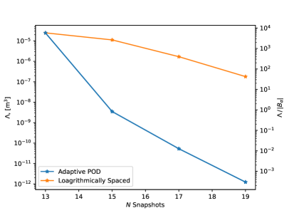
Figure 5: Magnetic Conducting Sphere: Sphere of radius $\alpha=1\times 10^{-3}$ m, conductivity $\sigma_{*}=1\times 10^{6}$ S/m, and permeability $\mu_{r}=32$ with $\Omega$ discretised using a mesh with 21 151 tetrahedra and 1275 prisms and uniform $p=3$ elements. Showing $\Lambda$ and $\Lambda/|B_{\alpha}|$ obtained against $N$ for adaptively chosen and logarithmically spaced SS frequencies.

7.2 Conducting and Magnetic Disks

In this section, we consider the MPT characterisation of thin conducting and magnetic disks with their circular face in the $x_{1}-x_{3}$ plane. We consider a disk with physical dimensions radius $r=10\times 10^{-3}$ m and thickness $h=1\times 10^{-3}$ m and start with $\mu_{r}=32$ and $\sigma_{*}=1\times 10^{6}$ S/m. The computational domain $\Omega$ consists of a dimensionless disk $B$ of radius $r/\alpha$, and thickness $h/\alpha$ with $\alpha=1\times 10^{-3}$ m placed centrally in the box $[-1000,1000]^{3}$. The geometric increasing methodology from Section 6 is applied to construct boundary layers for different values of $\mu_{r}$ at a target frequency of $\omega=1\times 10^{8}$ rad/s. Then, $N=13$ solutions are computed at logarithmically spaced SS frequencies in the range $1\times 10^{1}\leq\omega\leq 1\times 10^{8}$ rad/s using $TOL_{\Sigma}=1\times 10^{-6}$, resulting in $M=11$. This process results in a discretisation of 24 748 tetrahedra and 2995 prisms with $p=3$ giving converged solutions at the snapshots. Due to the symmetries of the disk, which, in addition to mirror symmetries, is rotationally symmetric around ${\bm{e}}_{2}$, the non-zero independent tensor coefficients associated with the object reduce to $({\mathcal{M}})_{11}=({\mathcal{M}})_{33}$ and $({\mathcal{M}})_{22}$ [25]. For this reason, in Figures 6 and 7 we show only $(\tilde{\mathcal{R}})_{11}=(\tilde{\mathcal{R}})_{33}$, $(\tilde{\mathcal{R}})_{22}$, $(\tilde{\mathcal{R}})_{12}=(\tilde{\mathcal{R}})_{23}=(\tilde{\mathcal{R}})_{13}=0$ and $({\mathcal{I}})_{11}=(\mathcal{I})_{33}$, $({\mathcal{I}})_{22}$, $({\mathcal{I}})_{12}=({\mathcal{I}})_{23}=({\mathcal{I}})_{13}=0$. The figures show excellent agreement between the IM and MM methodologies.

$\begin{array}[]{cc}\includegraphics[width=208.13599pt]{disk_thin_disk_tensor_comparison_real}&\includegraphics[width=208.13599pt]{disk_thin_disk_tensor_comparison_imag}\\ (a)&(b)\end{array}$

Figure 6: Thin Conducting Magnetic Disk: Disk of radius $10\times 10^{-3}$ m, height $1\times 10^{-3}$ m, conductivity $\sigma_{*}=1\times 10^{6}$ S/m, and permeability $\mu_{r}=32$ with $\Omega$ discretised using a mesh with 24 748 tetrahedra and 2995 prisms, uniform $p=3$ elements and $N=13$. Showing a comparison between the original IM and the new faster MM approach for the calculation of the MPT spectral signature $(a)$ $(\tilde{\mathcal{R}})_{ij}$ and $(b)$ $({\mathcal{I}})_{ij}$. On this scale, the MM and IM methods are indistinguishable.

To illustrate the adaptive procedure described by Algorithm 1, we show the spectral signature for $(\tilde{\mathcal{R}})_{ij}$ including the a-posteriori error certificates $(\tilde{\mathcal{R}}\pm\Delta)_{ij}$ obtained at different iterations for same magnetic disk in Figure 7. Starting with the setup used in Figure 6 and a stopping tolerance of $TOL_{\Delta}=1\times 10^{-3}$, we show the first 4 iterations of the adaptive algorithm resulting in $N=15,17,19$ non-logarithmically spaced snapshots, respectively, in the subsequent 3 iterations in a similar manner to the earlier sphere example. The convergence behaviour for certificates for $({\mathcal{I}}+\Delta)_{ij}$ is very similar and, therefore, not shown.

$\begin{array}[]{c c}\includegraphics[width=208.13599pt]{disk_disk_iter1}&\includegraphics[width=208.13599pt]{disk_disk_iter2}\\ (a)&(b)\\ \includegraphics[width=208.13599pt]{disk_disk_iter3}&\includegraphics[width=208.13599pt]{disk_disk_iter4}\\ (c)&(d)\end{array}$

Figure 7: Thin Conducting Permeable Disk: Disk of radius $10\times 10^{-3}$ m, height $1\times 10^{-3}$ m, conductivity $\sigma_{*}=1\times 10^{6}$ S/m, and permeability $\mu_{r}=32$ with $\Omega$ discretised using a mesh with 24 748 tetrahedra and 2995 prisms with uniform $p=3$ elements. Showing $(\tilde{\mathcal{R}})_{ij}$ and $(\tilde{\mathcal{R}}+\Delta)_{ij}$ obtained by applying Algorithm 1 for $(a)$ iteration 1, $N=13$, $(b)$ iteration 2, $N=15$, $(c)$ iteration 3, $N=17$ and $(d)$ iteration 4, $N=19$.

To illustrate the performance of the adaptive POD, compared to non-adaptive logarithmically spaced SS, Figure 8 shows the maximum error, $\Lambda$, against $N$, which, like the earlier sphere example, shows significant benefits of the adaptive scheme over logarithmically spaced SS.

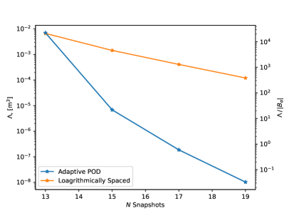
Figure 8: Thin Conducting Permeable Disk: Disk of radius $10\times 10^{-3}$ m, height $1\times 10^{-3}$ m, conductivity $\sigma_{*}=1\times 10^{6}$ S/m, and permeability $\mu_{r}=32$ with $\Omega$ discretised using a mesh with 24 748 tetrahedra and 2995 prisms with uniform $p=3$ elements. Showing $\Lambda$ and $\Lambda/|B_{\alpha}|$ obtained against $N$ for the first 4 iterations of adaptively chosen and logarithmically spaced SS frequencies.

Considering the limiting case of an infinitely thin conducting non-magnetic disk in the $x_{1}-x_{3}$ plane and the corresponding limiting case when the disk is magnetic, based on measurements observations for finitely thick disks [1, 35] (which is rotated to a disk in the $x_{1}-x_{2}$ plane for our situation), it has been proposed that the form of the MPT (when its coefficients are displayed as a matrix) undergo the transition

$$\mathcal{M}(\alpha B,\omega,\sigma_{*},1)=\begin{bmatrix}0&0&0\\ 0&c&0\\ 0&0&0\end{bmatrix}\to\mathcal{M}(\alpha B,\omega,\sigma_{*},\mu_{r}\to\infty)=\begin{bmatrix}m&0&0\\ 0&m&0\\ 0&0&0\end{bmatrix}$$

as $\mu_{r}$ becomes large. We would like to investigate the form this transition takes numerically for a finitely thick disk and wish to understand the impact of changing the $\mu_{r}$ value. Thus, we consider the same conducting permeable disk as in Figure 6, but now with $\mu_{r}=1,8,16,64$ in turn. In each case, different thickness prismatic layers were constructed according to the recipe in Section 6 for a target value of $\omega=1\times 10^{8}$ rad/s and then the MPT coefficients obtained by using a PODP method for $N=13$ snapshot solutions at logarithmically spaced frequencies in the range $1\times 10^{1}\leq\omega\leq 1\times 10^{8}$ rad/s and $TOL_{\Sigma}=1\times 10^{-6}$. We show the independent non-zero diagonal coefficients of $\tilde{\mathcal{R}}$ and ${\mathcal{I}}$. Interestingly, despite the relative simplicity of the geometry and its homogeneous materials, we observe the presence of multiple local maxima in $({\mathcal{I}})_{ij}$ for the cases of $\mu_{r}=16$ and $\mu_{r}=64$. This can be explained by the spectral theory of MPT spectral signatures [28] where, in this case, the first term in the expansions in Lemma 8.5 is no longer dominant and multiple terms play an important role.

$\begin{array}[]{c c}\includegraphics[width=208.13599pt]{disk_combined_real_i=j=3}&\includegraphics[width=208.13599pt]{disk_combined_imag_i=j=3}\\ (a)&(b)\\ \includegraphics[width=208.13599pt]{disk_combined_real_i=j=2}&\includegraphics[width=208.13599pt]{disk_combined_imag_i=j=2}\\ (c)&(d)\\ \end{array}$

Figure 9: Thin Conducting Permeable Disk: Disk of radius $10\times 10^{-3}$ m, height $1\times 10^{-3}$ m, conductivity $\sigma_{*}=1\times 10^{6}$ S/m, and varying permeability with $\Omega$ discretised using a mesh with 24 748 tetrahedra and 2995 prisms using $L=2$ prismatic layers and thickness according to geometric increasing methodology of Section 6 and uniform $p=3$ elements. Showing the effect of increasing $\mu_{r}=1,8,16,64$ with arrows indicating the evolution of the spectral signature with ($a$) $(\tilde{\mathcal{R}})_{11}=(\tilde{\mathcal{R}})_{33}$, ($b$) $(\mathcal{I})_{11}=({\mathcal{I}})_{33}$, ($c$) $(\tilde{\mathcal{R}})_{22}$, and ($d$) $(\mathcal{I})_{22}$.

7.3 Inhomogeneous Bomblet

One potential practical application is the MPT characterisation of unexploded ordnance, which may assist in allowing the land to be safely released for civilian use in areas of former conflict. A common type of ordnance is the near spherical bomblet (e.g. a BLU-26 submunition [11, 46]). This commonly consists of a die-cast aluminium shell, an explosive payload and fuze, aerodynamic flutes used to induce a rotation in the bomblet as it falls as part of the arming process, multiple (typically hundreds) small steel fragmentation balls, and a steel clamp ring [46]. As an example, Figure 10 shows photographs of a recovered bomblet shell, showing the metallic ring, remnants of the fragmentation balls that are cast in the shell, and flutes. See also Figure 1 in [46].

$\begin{array}[]{c c c}\includegraphics[width=138.75967pt]{bomblet_photo.png}&\includegraphics[width=138.75967pt]{bomblet_photo2.png}&\includegraphics[width=138.75967pt]{bomblet_photo3.png}\end{array}$

Figure 10: Recovered hemispherical bomblet shell part of diameter 6.3 cm. Images taken courtesy of the group of Professor A.J. Peyton, Department of Electrical and Electronic Engineering, The University of Manchester.

In the following we consider idealised models of the bomblet, first without fragmentation balls and then with them included. Throughout the following we make assumptions based on a sample part a BLU-26 bomblet and our understanding from the limited information openly available.

7.3.1 No Fragmentation Balls

While the flutes (which appear to be made of the same material as the shell [46]) are geometrically interesting (having a mirror symmetry and a 4-fold rotation symmetry [29]), with the steel clamp ring orientated in the same plane as the mirror symmetry, which we take to be ${x}_{1}-{x}_{2}$, the symmetries of this object imply the MPT will be diagonal with $(\mathcal{M})_{11}=(\mathcal{M})_{22}$ and $(\mathcal{M})_{33}$ as independent non-zero coefficients. But, given that the flutes make up only a small fraction of the overall volume, and removing them does not change which coefficients are independent, they are omitted. In this section, we consider two simplified idealised models: The first has a 3.14 cm radius a solid spherical aluminium ball with a steel clamp ring attached around the outside; the second is the same as the first but has a hollow spherical region of radius 2.4 cm.

To compute the MPT spectral signature of the first model, a computational domain $\Omega$ consisting of a dimensionless object $B$ made up of a sphere of radius $3.14$ cm joined to a clamp ring, which is modelled with radius $3.44$ cm and height $0.31$ cm, is centrally placed in a $[-100,100]^{3}$ non-conducting region. The physical object $B_{\alpha}$ is obtained from the non-dimensional object $B$ using a scaling of $\alpha=0.01$ m. The material parameters are chosen as $\mu_{r}=1$ and $\sigma_{*}=3\times 10^{7}$ S/m for the aluminium sphere and $\mu_{r}=200$, $\sigma_{*}=6\times 10^{6}$ S/m for the steel ring. Based on these materials, the resulting $\tau=\delta/\alpha$ at a maximum target frequency of $\omega=1\times 10^{8}$ rad/s for both materials is much smaller than those previously considered, making this problem considerably more challenging. For this reason, boundary layer elements are added to both the non-magnetic sphere, and the magnetic ring with thickness chosen according to $\tau$ for each material. In particular, the geometric increasing refinement strategy with $L=2$ layers is used resulting in a mesh with 29 141 unstructured tetrahedra, and 6355 prisms, which was found to be converged at SS frequencies using uniform $p=4$ elements, resulting in a problem with $N_{d}\approx 1.23\times 10^{6}$. Due to the complexity and size of this object, we have increased the regularisation to $\varepsilon=1\times 10^{-8}$ and the iterative solver tolerance to $TOL=1\times 10^{-7}$. For the POD, $N=13$ logarithmically spaced frequency SS was employed using $TOL_{\Sigma}=1\times 10^{-6}$ and the resulting MPT signature obtained by applying the adaptive Algorithm 1 after 4 iterations, where $M=19$ and $TOL_{\Delta}=10^{-3}$, are compared in Figure 11.

The figure shows that the initial logarithmically spaced snapshots are in good agreement with the additional adaptively introduced snapshots and that the addition of new full order solutions does not significantly change the approximate tensor coefficients obtained by the POD method. The MPT spectral signature of the hollow bomblet, which is also shown, was obtained in a similar way using a discretisation with 30 379 tetrahedra and 8115 prisms and the same settings as before. As shown in the figure, The solid bomblet provides a good approximation for the hollow example. This agreement improves with frequency due to the decreasing skin depth and reduced contribution from the cavity.

$\begin{array}[]{c c}\includegraphics[width=208.13599pt]{bomblet_real_hollow_solid_comparison}&\includegraphics[width=208.13599pt]{bomblet_imag_hollow_solid_comparison}\\ (a)&(b)\end{array}$

Figure 11: Conducting Magnetic Bomblet: Comparison between a solid and hollow bomblet consisting of a non-magnetic spherical core of radius 3.14 cm, with material properties $\mu_{r}=1,\sigma_{*}=3\times 10^{7}$ S/m, and a magnetic ring of radius 3.44 cm and height 0.31 cm with $\mu_{r}=200,\sigma_{*}=6\times 10^{6}$ S/m with $\Omega$ discretised by 29 141 tetrahedra and 6355 prisms for the solid example and 30 379 tetrahedra and 8115 prisms for the hollow example using uniform $p=4$ elements. Due to the symmetries of the object $(\mathcal{M})_{11}=(\mathcal{M})_{22}$ and $(\mathcal{M})_{12}=(\mathcal{M})_{13}=(\mathcal{M})_{23}=0$ thus we only show only ($a$) $(\tilde{\mathcal{R}})_{11}=(\tilde{\mathcal{R}})_{22}$, $(\tilde{\mathcal{R}})_{33}$ and ($b$) $(\mathcal{I})_{11}=(\mathcal{I})_{22}$, $(\mathcal{I})_{33}$, obtained using the MM approach and adaptive schemes with SS solutions also superimposed.

We show contours of the computed $|{\rm Re}({\bm{\theta}}_{2}^{(1,hp)})|$ (normalised to $[0,1]$ to ease comparison) that are obtained as part of the solution process at the fixed frequencies $\omega=1\times 10^{2},1\times 10^{4}$, and $1\times 10^{6}$ rad/s in Figure 12. The figure shows the contours on a plane chosen to be perpendicular to ${\bm{e}}_{3}$, highlighting the decay of the fields inside the object as skin depth decreases. We use the same mesh, as the earlier discussion, however, we have increased the order to $p=5$ in order ensure a fine resolution of the field, which was not necessary for the MPT spectral signature due to the averaging through volume integration. The results highlight the extremely small skin depths associated with the higher frequencies, and that the fields concentrate along the magnetic ring, although in the case of $\omega=1\times 10^{2}$ rad/s the wavelength is too large to induce significant eddy currents in the ring.

$\begin{array}[c]{c c c c}\includegraphics[width=124.88441pt]{bomblet_om=1e2_cropped}&\includegraphics[width=124.88441pt]{bomblet_om=1e4_cropped}&\includegraphics[width=124.88441pt]{bomblet_om=1e6_cropped}&\includegraphics[width=32.38031pt]{bomblet_colormap}\\ (a)&(b)&(c)\end{array}$

Figure 12: Conducting Magnetic Bomblet: Contours of $\lvert{\rm Re}({\bm{\theta}}_{2}^{(1,hp)})\rvert$ (normalised to $[0,1]$) for $(a)$ $\omega=1\times 10^{2}$ rad/s, $(b)$ $\omega=1\times 10^{4}$ rad/s, and $(c)$ $\omega=1\times 10^{6}$ rad/s. Results shown on a bisecting plane perpendicular to the unit vector ${\bm{e}}_{3}$.

7.3.2 With Fragmentation Balls

Next we consider the case where steel fragmentation balls are included in the hollow bomblet. We believe that they are cast in to the aluminium shell, although we are not certain of this. We also do not know the number of balls, their size, or their location inside the bomblet. For our model, we have assumed that they are 2mm in radius and are placed approximately equidistant from each other throughout a layer adjacent to the interior of the shell. The properties of the balls are also unknown, but they are likely to be made of steel. We assume that they have material parameters $\mu_{r}=200$, $\sigma_{*}=6\times 10^{6}$ S/m as per the assumed steel for the clamp ring. Importantly, introducing these fragmentation balls breaks the mirror and rotational symmetries of the bomblet, and so the MPT now has 6 independent coefficients as a function of $\omega$.

We consider models with 100, 200, and 400 fragmentation balls which, given their size relative to the bomblet diameter, cannot be easily resolved without introducing an extremely large number of additional elements in the mesh or using a special geometrical techniques such as a NURB enhanced finite elements [44]. Given the aforementioned assumptions and approximations, we instead use an $L_{2}$ projection to project the expected varying distribution of $\mu_{r}$ and $\sigma_{*}$ on to piecewise constant materials for a mesh consisting of 33 410 tetrahedra and 9 063 prisms.

To show the effect of increasing the number of fragmentation balls, we show a comparison between the hollow bomblet used for Figure 11, the addition of a steel layer in the interior shell and alternatively the addition of a layer with 100, 200, and 400 fragmentation balls. The effect of increasing the number of fragmentation balls is shown in Figure 13 where $(\tilde{\mathcal{R}})_{11}$, $({\mathcal{I}})_{11}$, $(\tilde{\mathcal{R}})_{12}$, and $({\mathcal{I}})_{12}$ are shown as a sample of the 6 independent coefficients. The figure shows an increase in magnitude from the hollow bomblet solution towards the layered bomblet solution for the on-diagonal entries and the generation of off-diagonal terms in the MPT when the fragmental balls are added due to the breaks in the previous symmetries for the hollow and layered bomblets. The inclusion of the balls has important effects on the MPT signature and these differences may be useful when undertaking object classification.

$\begin{array}[]{c c}\includegraphics[width=208.13599pt]{bomblet_R11_balls_comparison_4mm}&\includegraphics[width=208.13599pt]{bomblet_I11_balls_comparison_4mm}\\ (a)&(b)\\ \includegraphics[width=208.13599pt]{bomblet_R12_balls_comparison_4mm}&\includegraphics[width=208.13599pt]{bomblet_I12_balls_comparison_4mm}\\ (c)&(d)\\ \end{array}$

Figure 13: Conducting Magnetic Bomblet: Idealised bomblet consisting of a solid non-magnetic spherical core of radius 3.14 cm, with material properties $\mu_{r}=1,\sigma_{*}=3\times 10^{7}$ S/m, and a magnetic ring of radius 3.44 cm and height 0.31 cm with $\mu_{r}=200,\sigma_{*}=6\times 10^{6}$ S/m. Comparison between the hollow bomblet example, and the inclusion of either a solid layer of steel ($\mu_{r}=200,\sigma_{*}=6\times 10^{6}$ S/m) or 100, 200, and 400 steel fragmentation balls. Figure shows ($a$) $(\tilde{\mathcal{R}})_{11}$, ($b$) $(\mathcal{I})_{11}$, ($c$) $(\tilde{\mathcal{R}})_{21}$, and ($d$) $({\mathcal{I}})_{21}$. Note that all 6 coefficients of $\tilde{\mathcal{R}}$ and $\mathcal{I}$ are independent when fragmentation balls are added.

7.3.3 Timings

As an illustration of timings for the challenging bomblet example, we consider the solid bomblet from Section 7.3.1 and note the computations savings reported here also carry over to the other bomblet models and other challenging examples in general. Timings were performed using workstation 2 described in Section 5 with comparisons made for IM and MM for the MPT coefficient computation in the POD scheme. In Figure 14, we show the wall clock timing break down for the aforementioned setup, accelerated with the use of multi-threading as previously described in Section 5 and 2 multiprocessing cores. The timing is broken down in to the off-line stage of generating the mesh, computing the solution coefficients for the ${\bm{\theta}}_{i}^{(0,hp)}$, computing the solution coefficients for the ${\bm{\theta}}_{i}^{(1,hp)}$ snapshots, and computing the ROM (in which the TSVDs are obtained), and an on-line stage consisting of solving the smaller linear systems (16) and computing the tensor coefficients. Comparing the IM and MM approaches, we see a significant saving in the final stage of computing the MPT coefficients, which, for this particular discretisation, required approximately $6\times 10^{4}$ seconds using the IM. In comparison, the computation of the MPT coefficients for the MM becomes negligible and reduces the overall computation to around $2\times 10^{4}$ seconds. There is an additional memory overhead in the MM approach, which is associated with the building of the larger matrices ${\mathbf{K}}$, ${\mathbf{C}}$, ${\mathbf{C}}^{(1)}$ and ${\mathbf{C}}^{(2)}$ of dimension $N_{d}\times N_{d}$ if $M_{d}=N_{d}$, which can be incorporated to the off-line stage of the ROM if desired. The on-line stage of the ROM only requires the smaller dimension matrices of size at most $M\times M$ with $M\ll N_{d}$ and the larger matrices can be disposed off once ${\mathbf{U}}_{i}^{M}$ are available. Nevertheless, this additional memory overhead is still less than the peak memory requirements during the computation of the solution coefficients for the ${\bm{\theta}}_{i}^{(1,hp)}$ snapshots and so it is not of concern.

$\begin{array}[]{c c}\includegraphics[width=208.13599pt]{bomblet_Timings_bomblet_p=4_int_increased_reg_22_06_23}&\includegraphics[width=208.13599pt]{bomblet_Timings_bomblet_p=4_mat_increased_reg_22_06_23}\\ (a)&(b)\end{array}$

Figure 14: Conducting Magnetic Bomblet: Idealised bomblet consisting of a solid non-magnetic spherical core of radius 3.14 cm, with material properties $\mu_{r}=1,\sigma_{*}=3\times 10^{7}$ S/m, and a magnetic ring of radius 3.44 cm and height 0.31 cm with $\mu_{r}=200,\sigma_{*}=6\times 10^{6}$ S/m with $\Omega$ discretised by 29 141 tetrahedra and 6355 prisms and uniform $p=4$ elements. Showing timing results for $(a)$ IM, and $(b)$ MM methods.

8 Conclusions

In this paper, we developed a new computational formulation for efficiently computing MPT coefficients from POD predictions. This, in turn, has led to significant computational savings associated with obtaining MPT spectral signature characterisations of complex and highly magnetic conducting objects including magnetic disks of varying magnetic permeability and an idealised bomblet geometry. We have included timings to demonstrate the improvement in performance.

The paper has proposed a significant enhancement to our previous POD scheme by incorporating adaptivity where we choose new snapshot frequencies based on an a–posteriori error estimate computed, which is obtained at negligible computational cost. This adaptive method has been shown to provide an efficient way of choosing new frequency snapshots that leads in smaller a–posteriori error estimates compared to using the same number of logarithmically spaced frequency snapshots. The adaptive scheme is particularly useful for further refining the number and location of frequency snapshots given an initial set of logarithmically spaced snapshots.

In addition, we have significantly extended our earlier work [16] and provided a simple recipe to determine the number and thicknesses of prismatic boundary layers so as to achieve accurate solutions under $p$–refinement. By considering a magnetic sphere (for which an exact solution is known), we have shown that by choosing suitable thicknesses of 2 layers of prismatic elements and $p$–refinement was sufficient to achieve a relative error $E<1\times 10^{-3}$ for the MPT over a wide range of skin depths associated with materials and frequency excitations.

We have also included challenging realistic numerical examples that show the importance of using prismatic layers and the increased efficiency and improved accuracy of our new MPT calculation formulation.

We expect the procedures presented in this work to be invaluable for constructing large dictionaries of MPT characterisations of complex in-homogeneous realistic metallic objects. We also expect that the presented formulations for the adaptive POD, boundary layer construction, and the efficient post-processing to be transferable to the computation of GMPT object characterisations.

9 Acknowledgements

The authors would like to thank Prof. Peyton, Prof. Lionheart and Dr Davidson for their helpful discussions and comments on polarizability tensors. The authors are grateful for the financial support received from the Engineering and Physical Science Research Council (EPSRC, U.K.) through the research grant EP/V009028/1. Both authors would also like to thank the Isaac Newton Institute for Mathematical Sciences, Cambridge, for their support and hospitality during the programme Rich and Non-linear Tomography - a multidisciplinary approach where work on this paper was undertaken and related support from EPSRC grant EP/R014604/1.

References

- [1] Abdel-Rehim, O. A., Davidson, J. L., Marsh, L. A., O’Toole, M. D., and Peyton, A. J. Magnetic polarizability tensor spectroscopy for low metal anti-personnel mine surrogates. IEEE Sensors 16 (2016), 3775–3783.
- [2] Ambruš, D., Vasić, D., and Bilas, V. Robust estimation of metal target shape using time-domain electromagnetic induction data. IEEE Transactions Instrumentation and Measurement 65 (2016), 795–807.
- [3] Ammari, H., Chen, J., Chen, Z., Garnier, J., and Volkov, D. Target detection and characterization from electromagnetic induction data. Journal de Mathématiques Pures et Appliquées 101(1) (2014), 54–75.
- [4] Ammari, H., Chen, J., Chen, Z., Volkov, D., and Wang, H. Detection and classification from electromagnetic induction data. Journal of Computational Physics 301 (2015), 201–217.
- [5] Ao, C. O., Braunisch, H., O’Neill, K., and Kong, J. A. Quasi-magnetostatic solution for a conducting and permeable spheroid with arbitrary excitation. IEEE Transactions on Geoscience and Remote Sensing 40 (2002), 887–897.
- [6] Balanis, C. A. Advanced Engineering Electromagnetics, 2nd ed. CourseSmart Series. Wiley, Hoboken, NJ, USA, 2012.
- [7] Barrowes, B. E., O’Neill, K., Gregorcyzk, T. M., and Kong, J. A. Broadband analytical magnetoquasistatic electromagnetic induction solution for a conducting and permeable spheroid. IEEE Transactions on Geoscience and Remote Sensing 42 (2004), 2479–2489.
- [8] Baum, C. E. Low frequency near field magnetic scattering from highly, but not perfectly. Tech. Rep. 499, 1993.
- [9] Bjorck, A. Numerical Methods for Least Squares Problems. SIAM, Philadelphia, USA, 1996.
- [10] Ciarlet, P. Finite Element Method for Elliptic Equations. SIAM (2nd edition), 2002.
- [11] Collective Awareness to UXO. Cat-uxo - blu 26 submunition. https://cat-uxo.com/explosive-hazards/submunitions/blu-26-submunition. Accessed: 19/06/2023.
- [12] Davidson, J. L., Abdel-Rehim, O. A., Hu, P., Marsh, L. A., O’Toole, M. D., and Peyton, A. J. On the magnetic polarizability tensor of US coinage. Measurement Science and Technology 29 (2018), 035501.
- [13] Dekdouk, B., Ktistis, C., Marsh, L. A., Armitage, D. W., and Peyton, A. J. Towards metal detection and identification for humanitarian demining using magnetic polarizability tensor spectroscopy. Measurement Science and Technology 26 (2015), 115501.
- [14] Dohrmann, C. R. A preconditioner for substructuring based on constrained energy minimization. SIAM Journal of Scientific Computing 25, 1 (2003), 246–258.
- [15] Elgy, J., Ledger, P. D., Davidson, J. L., Özdeğer, T., and Peyton, A. J. Computations and measurements of the magnetic polarizability tensor characterisation of highly conducting and magnetic objects. Submitted (2022).
- [16] Elgy, J., Ledger, P. D., Davidson, J. L., and T. Özdeger. Computations and measurements of the magnetic polarizability tensor characterisation of high conducting and magnetic objects. Submitted.
- [17] Fernández, J. P., Barrowes, B., O’Neill, K., Paulsen, K., Shamatava, I., Shubitidze, F., and Sun, K. Evaluation of SVM classification of metallic objects based on a magnetic-dipole representation. Detection and Remediation Technologies for Mines and Minelike Targets XI 6217, June (2006), 621703.
- [18] Gabbay, J. E., and Scott, W. R. Wideband models for the electromagnetic induction signatures of thin conducting shells. IEEE Transactions on Geoscience and Remote Sensing 57, 10 (2019), 7330–7338.
- [19] Golub, G. H., and Loan, C. F. V. Matrix Computations. JHU Press, 1996.
- [20] Gregorcyzk, T. M., Zhang, B., Kong, J. A., Barrowes, B. E., and O’Neill, K. Electromagnetic induction from highly permeable and conductive ellipsoids under arbitrary excitation: application to the detection of unexploded ordances. IEEE Transactions on Geoscience and Remote Sensing 46 (2008), 1164–1176.
- [21] Hansen, P. C. Rank-Deficient and Discrete Ill-Posed Problems: Numerical Aspects of Linear Inversion. SIAM, Philadelphia, USA, 2005.
- [22] Hesthaven, J. S., Stamm, B., and Zhang, S. Efficient greedy algorithms for high-dimensional parameter spaces with applications to empirical interpolation and reduced basis methods. ESAIM: Mathematical Modelling and Numerical Analysis 48, 1 (2014), 259–283.
- [23] Karimian, N., O’Toole, M. D., and Peyton, A. J. Electromagnetic tensor spectroscopy for sorting of shredded metallic scrap. In IEEE SENSORS 2017 - Conference Proceedings (2017), IEEE.
- [24] Landau, L., Lifshitz, E., and L.P.Pitaevskii. Electrodynamics of Continuous Media. 1984.
- [25] Ledger, P. D., and Lionheart, W. R. B. Characterising the shape and material properties of hidden targets from magnetic induction data. IMA Journal of Applied Mathematics 80(6) (2015), 1776–1798.
- [26] Ledger, P. D., and Lionheart, W. R. B. An explicit formula for the magnetic polarizability tensor for object characterization. IEEE Transactions on Geoscience and Remote Sensing 56(6) (2018), 3520–3533.
- [27] Ledger, P. D., and Lionheart, W. R. B. Generalised magnetic polarizability tensors. Mathematical Methods in the Applied Sciences 41 (2018), 3175–3196.
- [28] Ledger, P. D., and Lionheart, W. R. B. The spectral properties of the magnetic polarizability tensor for metallic object characterisation. Mathematical Methods in the Applied Sciences 43 (2020), 78–113.
- [29] Ledger, P. D., and Lionheart, W. R. B. Minimal object characterisations using harmonic generalised polarizability tensors and symmetry groups. SIAM Journal on Applied Mathematics 82 (6) (2022), 2057–2079.
- [30] Ledger, P. D., Wilson, B. A., Amad, A. A. S., and Lionheart, W. R. B. Identification of metallic objects using spectral magnetic polarizability tensor signatures: Object characterisation and invariants. International Journal for Numerical Methods in Engineering 122 (2021), 3941–3984.
- [31] Ledger, P. D., Wilson, B. A., and Lionheart, W. R. B. Identification of metallic objects using spectral magnetic polarizability tensor signatures: Object classification. International Journal for Numerical Methods in Engineering 123 (2022), 2076–2111.
- [32] Ledger, P. D., and Zaglmayr, S. -finite element simulation of three-dimensional eddy current problems on multiply connected domains. Computer Methods in Applied Mechanics and Engineering 199 (2010), 3386–3401.
- [33] Makkonen, J., Marsh, L. A., Vihonen, J., Järvi, A., Armitage, D. W., Visa, A., and Peyton, A. J. KNN classification of metallic targets using the magnetic polarizability tensor. Measurement Science and Technology 25 (2014), 055105.
- [34] Makkonen, J., Marsh, L. A., Vihonen, J., Järvi, A., Armitage, D. W., Visa, A., and Peyton, A. J. Improving reliability for classification of metallic objects using a WTMD portal. Measurement Science and Technology 26 (2015), 105103.
- [35] Marsh, L. A., Ktisis, C., Järvi, A., Armitage, D. W., and Peyton, A. J. Three-dimensional object location and inversion of the magnetic polarisability tensor at a single frequency using a walk-through metal detector. Measurement Science and Technology 24 (2013), 045102.
- [36] Marsh, L. A., Ktistis, C., Järvi, A., .Armitage, D. W., and Peyton, A. J. Determination of the magnetic polarizability tensor and three dimensional object location for multiple objects using a walk-through metal detector. Measurement Science and Technology 25 (2014), 055107.
- [37] Özdeg̃er, T., Ledger, P. D., Lionheart, W. R. B., and Peyton, A. J. Measurement of GMPT coefficients for improved object characterisation in metal detection. IEEE Sensors Journal (2021). Accepted, DOI:10.1109/JSEN.2021.3133950.
- [38] Özdeğer, T. Advances in Techniques for the Characterisation of Targets in Metal Detection and Ultrawide Band Electromagnetic Screening Applications. Phd thesis, The University of Manchester, 2022.
- [39] Rehim, O. A. A., Davidson, J. L., Marsh, L. A., O’Toole, M. D., Armitage, D., and Peyton, A. J. Measurement system for determining the magnetic polarizability tensor of small metallic targets. In IEEE Sensor Application Symposium (2015).
- [40] Schöberl, J. NETGEN - an advancing front 2D/3D-mesh generator based on abstract rules. Computing and Visualization in Science 1(1) (1997), 41–52.
- [41] Schöberl, J. C++11 implementation of finite elements in NGSolve. Tech. rep., ASC Report 30/2014, Institute for Analysis and Scientific Computing, Vienna University of Technology, 2014.
- [42] Schöberl, J., and Zaglmayr, S. High order Nédélec elements with local complete sequence properties. COMPEL-The International Journal for Computation and Mathematics in Electrical and Electronic Engineering 24(2) (2005), 374–384.
- [43] Schwab, C., and Suri, M. The and versions of the finite element method for problems with boundary layers. Mathematics of Computation 65 (1996), 1403–1429.
- [44] Sevilla, R., Fernández-Méndez, S., and Huerta, A. NURBS-enhanced finite element method (NEFEM). Archives of Computational Methods in Engineering 18, 4 (2011), 441–484.
- [45] Song, L. P., Billings, S. D., Pasion, L. R., and Oldenburg, D. W. Transient electromagnetic scattering of a metallic object buried in underwater sediments. IEEE Transactions on Geoscience and Remote Sensing 54, 2 (2016), 1091–1102.
- [46] United States Air Force. Review Of BLU-63 / B bomblet program: B-173803. Tech. rep., United States Air Force, Washington, D.C, USA, 1972.
- [47] Wait, J. R. A conducting sphere in a time varying magnetic field. Geophysics 16(4) (1951), 666–672.
- [48] Wait, J. R. On the electromagnetic response of a conducting sphere to a dipole field. Geophysics 25 (1960), 569–687.
- [49] Wilson, B. A., and Ledger, P. D. Efficient computation of the magnetic polarizabiltiy tensor spectral signature using proper orthogonal decomposition. International Journal for Numerical Methods in Engineering 122, 8 (2021), 1940–1963.
- [50] Zaglmayr, S. High Order Finite Elements for Electromagnetic Field Computation. PhD thesis, Johannes Kepler University Linz, 2006.
- [51] Zhao, Y., Yin, W., Ktistis, C., Butterworth, D., and Peyton, A. J. Determining the electromagnetic polarizability tensors of metal objects during in-line scanning. IEEE Transactions on Instrumentation and Measurement 65 (2016), 1172–1181.