Channel State Information-Free Location-Privacy Enhancement: Fake Path Injection

Abstract

In this paper, a channel state information-free, fake path injection (FPI) scheme is proposed for location-privacy preservation. Specifically, structured artificial noise is designed to introduce virtual fake paths into the channels of the illegitimate devices. By leveraging the geometrical feasibility of the fake paths, under mild conditions, it can be proved that the illegitimate device cannot distinguish between a fake and true path, thus degrading the illegitimate devices’ ability to localize. Two closed-form, lower bounds on the illegitimate devices’ estimation error are derived via the analysis of the Fisher information of the location-relevant channel parameters, thus characterizing the enhanced location-privacy. A transmit beamformer is proposed, which efficiently injects the virtual fake paths. The intended device receives the two parameters of the beamformer design over a secure channel in order to enable localization. The impact of leaking the beamformer structure and associated localization leakage are analyzed. Theoretical analyses are verified via simulation. Numerical results show that a $20$dB degradation of the illegitimate devices’ localization accuracy can be achieved thus validating the efficacy of the proposed FPI versus using unstructured Gaussian noise.

I Introduction

With the wide deployment of the Internet-of-Things, location of user equipment (UE) is becoming an important commodity. The proliferation of wearables and the associated location-based services necessitate location-privacy preservation. Unfortunately, most existing works on localization, such as [2, 3, 4], focus on how to leverage the features of the wireless signals to improve estimation accuracy without considering location-privacy. These wireless signals that have the confidential location information embedded in them are easily exposed to the risk of eavesdropping, i.e., illegitimate devices can determine the locations of the UE when the UEs request the location-based services from legitimate devices. Even worse, more private information, such as age, gender, and personal preference, can be snooped and inferred from the leaked location information as well [5]. Hence, it is critical to develop new strategies to limit location-privacy leakage (LPL).

To combat eavesdropping, location-privacy preservation has predominantly been studied at the application and network layers [6, 7, 8]. To the best of our knowledge, enabling physical-layer signals for protecting the location-privacy of UEs has not been fully investigated. Due to the nature of the propagation of electromagnetic waves, as long as the illegitimate devices can listen to the wireless channel and leverage the received signals for localization, the location-privacy of the UE is inevitably jeopardized. Traditionally, to preserve the location-privacy at the physical layer, the statistics of the channel, or the actual channel, have been exploited to prevent the illegitimate devices from easily extracting the location-relevant information from the wireless signals [9, 10, 11, 5]. Example strategies include artificial noise injection [9, 10] and beamforming design [11, 5]. More precisely, to make the malicious localization harder, via artificial noise, the received signal-to-noise ratio (SNR) can be decreased for illegitimate devices; to maintain the legitimate localization accuracy, actual noise realizations have to be shared with the legitimate devices or the channel state information (CSI) is known to the UE so as to inject the artificial noise into the null space of the legitimate channel [9, 10]. On the other hand, if Alice has prior knowledge of the CSI for the illegitimate channel, the transmit beamformer can be specifically designed to hide the key location-relevant information [11, 5]. In particular, by exploiting the CSI to design a transmit beamformer, [5] misleads the illegitimate device into incorrectly treating one non-line-of-sight (NLOS) path as the line-of-sight (LOS) path such that UE’s position cannot be accurately inferred, where the obfuscation is achieved by adding a delay for the transmission over the LOS path. However, all these existing physical-layer security designs [9, 10, 11, 5] highly rely on accurate or even perfect CSI and thus are costly.

In the sequel, motivated by the analysis of the structure of the channel model in [12, 13, 4, 14], we propose a fake path injection (FPI)-aided location-privacy enhancement scheme to reduce location privacy leakage to illegitimate devices. A provably, statistically hard estimation problem is created, while providing localization guarantees to legitimate devices. In contrast to [9, 11, 10, 5], our design does not require CSI, which avoids extra channel estimation and reduces the overhead for resource-limited UEs.

The main contributions of this paper are:

• A general framework for FPI-aided location-privacy enhancement is proposed without CSI, where the intrinsic structure of the channel is explicitly exploited to design the fake paths.

• The identifiability of the designed fake paths is investigated. The analysis indicates that the illegitimate devices cannot provably distinguish and remove the fake paths.

• In the presence of the proposed fake paths, two closed-form, lower bounds on the estimation error are derived for the illegitimate devices, suggesting appropriate values of key design parameters to enhance location-privacy.

• A beamforming strategy is designed to efficiently inject the fake paths, where LPL is mitigated, while the securely shared information (a secret key [15, 16, 17, 18]) is characterized to maintain authorized devices’ localization accuracy. Only two parameters need to be shared with the legitimate device. The potential leakage of the beamformer structure is also studied for the robustness of the proposed scheme.

• Theoretical analyses are validated via simulation and numerical comparisons of the localization accuracy of legitimate devices. The proposed method can contribute to $20$dB localization accuracy degradation for illegitimate devices even when the LOS path exists. If the structure of the designed beamformer is unfortunately leaked, there is still around a $4$dB accuracy degradation for the illegitimate device. This degradation can be increased by creating more complex beamformers.

• For low SNRs, the proposed scheme is numerically shown to be more effective for location-privacy preservation, than the injection of unstructured Gaussian noise, which requires the sharing of entire noise realizations.

The present work completes our previous work [1] with an analysis of identifiability of the designed fake paths, which ensures that the fake paths are challenging for the illegitimate devices to remove. In addition, considering the injected fake paths, we derive two closed-form, lower bounds on the estimation error based on the Fisher information of the location-relevant channel parameters. Our work is different from the analysis of the stability of the super-resolution problem [19, 20, 21, 22] with the goal of guaranteeing high estimation accuracy with a certain statistical resolution limit at high SNR. In contrast, our lower bounds are to validate that estimation accuracy can be efficiently degraded for an eavesdropper, if the injected fake paths are close to the true paths in terms of the location-relevant parameters. We note that, in the presence of noise, the stability of the Fisher information matrix (FIM) of the line spectral estimation problem has been studied (see e.g. [23]) for a new algorithm-free resolution limit; our analysis is tailored to location-privacy preserving design with multi-dimensional signals.

The rest of this paper is organized as follows. Section II introduces the signal model adopted for localization. Section III presents the proposed CSI-free location-privacy enhancement framework, with the fake paths designed according to the intrinsic channel structure. In Section IV, the identifiability of the injected fake paths is investigated to show that such fake paths cannot be removed. In the presence of the fake paths, two closed-form, lower bounds on the estimation error are derived and analyzed in Section V, proving the efficacy of the proposed scheme. Section VI proposes a transmit beamformer to practically inject the designed fake paths. The beamformer design does not rely on CSI. Numerical results are provided in Section VII to validate the theoretical analyses and highlight the performance degradation caused by the FPI to the eavesdropper. Conclusions are drawn in Section VIII. Appendices A, B, C, and E provide the proofs for the key technical results.

We use the following notation. Scalars are denoted by lower-case letters $x$ and column vectors by bold letters $\bm{x}$. The $i$-th element of $\bm{x}$ is denoted by $\bm{x}[i]$. Matrices are denoted by bold capital letters $\bm{X}$ and $\boldsymbol{X}[i,j]$ is the ($i$, $j$)-th element of $\bm{X}$. The operators $\lfloor{x}\rfloor$, $|x|$, $\|\bm{x}\|_{2}$, $\mathfrak{R}\{x\}$, $\mathfrak{I}\{x\}$, and $\operatorname{diag}(\mathcal{A})$ represent the largest integer that is less than or equal to $x$, the magnitude of $x$, the $\ell_{2}$ norm of $\bm{x}$, the real part of $x$, the imaginary part of $x$, and a diagonal matrix whose diagonal elements are given by $\mathcal{A}$, respectively. $\boldsymbol{I}_{l}$ stands for a $l\times l$ identity matrix and $\mathbb{P}(\cdot)$ is reserved for the probability of an event. The operators $\mathbb{E}\{\cdot\}$ denotes the expectation of a random variable. The operators $\operatorname{Rank}(\cdot)$, $\operatorname{Tr}(\cdot)$, $\operatorname{det}(\cdot)$, $(\cdot)^{\mathrm{T}}$, and $(\cdot)^{\mathrm{H}}$ are defined as the rank of a matrix, the trace of a matrix, the determinant of a matrix, the transpose of a matrix or vector, and the conjugate transpose of a vector or matrix, respectively.

II System Model

We consider a legitimate device (Bob) serving a UE (Alice), as shown in Figure 1. The locations of Alice and Bob are denoted by $\bm{p}=[p_{x},p_{y}]^{\mathrm{T}}\in\mathbb{R}^{2}$ and $\bm{q}=[q_{x},q_{y}]^{\mathrm{T}}\in\mathbb{R}^{2}$, respectively. To acquire location-based services, Alice transmits pilot signals to Bob, while Bob estimates Alice’s position based on the received signals and his location $\bm{q}$. We assume that the pilot signals are known to Bob. An illegitimate device (Eve) exists at location $\bm{z}=[z_{x},z_{y}]^{\mathrm{T}}\in\mathbb{R}^{2}$. Eve also knows the same pilot signals and her location $\bm{z}$. By eavesdropping on the channel to infer $\bm{p}$, Eve jeopardizes Alice’s location-privacy.

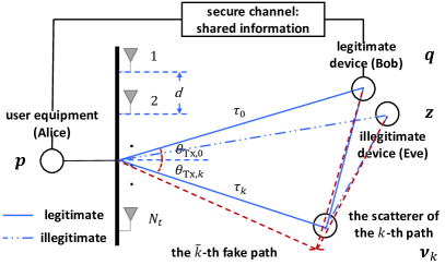
Figure 1: System model.

Without of loss of generality, we adopt the millimeter-wave (mmWave) multiple-input-single-output (MISO) orthogonal frequency-division multiplexing (OFDM) channel model of [24] for transmissions, where Alice is equipped with $N_{t}$ antennas, while both Bob and Eve have a single antenna. Assume that $K+1$ paths, i.e., one LOS path and $K$ NLOS paths, exist in the MISO OFDM channel, and the scatterer of the $k$-th NLOS path is located at an unknown position $\bm{v}_{k}=[v_{k,x},v_{k,y}]^{\mathrm{T}}\in\mathbb{R}^{2}$, for $k=1,2,\cdots,K$. We transmit $G$ OFDM pilot signals via $N$ sub-carriers with central carrier frequency $\varphi_{c}$ and bandwidth $B$. It is assumed that a narrowband channel is employed, i.e., $B\ll\varphi_{c}$. Denoting by $x^{(g,n)}$ and $\bm{f}^{(g,n)}\in\mathbb{C}^{N_{t}\times 1}$ the $g$-th symbol transmitted over the $n$-th sub-carrier and the corresponding beamforming vector, respectively, we can express the $g$-th pilot signal over the $n$-th sub-carrier as $\boldsymbol{s}^{(g,n)}\triangleq\bm{f}^{(g,n)}x^{(g,n)}\in\mathbb{C}^{N_{t}\times 1}$ and write the received signal ${y}^{(g,n)}$ as

$${y}^{(g,n)}=\boldsymbol{h}^{(n)}\boldsymbol{s}^{(g,n)}+{w}^{(g,n)},$$ (1)

for $n=0,1,\cdots,N-1$ and $g=1,2,\cdots,G$, where ${w}^{(g,n)}\sim\mathcal{CN}({0},\sigma^{2})$ is an independent, zero-mean, complex Gaussian noise with variance $\sigma^{2}$, and $\bm{h}^{(n)}\in\mathbb{C}^{1\times N_{t}}$ represents the $n$-th sub-carrier public channel vector. We assume that the pilot signals transmitted over the $n$-th sub-carrier are independent and identically distributed and $\mathbb{E}\{\boldsymbol{s}^{(g,n)}(\boldsymbol{s}^{(g,n)})^{\mathrm{H}}\}=\frac{1}{N_{t}}\bm{I}_{N_{t}}$ holds for any $g$ and $n$. Denote by $c$, $d$, $T_{s}$ and $\bm{a}_{L}(f)\in\mathbb{C}^{L}$ the speed of light, the distance between antennas, the sampling period $T_{s}\triangleq\frac{1}{B}$, and the unit-norm Fourier vector $\bm{a}_{L}(\vartheta)\triangleq\frac{1}{\sqrt{L}}\left[1,e^{-j2\pi\vartheta},\dots,e^{-j2\pi(L-1)\vartheta}\right]^{\mathrm{T}}$, respectively. The public channel vector $\bm{h}^{(n)}$ is defined as

$$\boldsymbol{h}^{(n)}\triangleq\sqrt{N_{t}}\sum_{k=0}^{K}\gamma_{k}e^{\frac{-j2\pi n\tau_{k}}{NT_{s}}}\boldsymbol{\alpha}\left(\theta_{\mathrm{Tx},k}\right)^{\mathrm{H}},$$ (2)

where $k=0$ corresponds to the LOS path, $\gamma_{k}$ represents the complex channel coefficient of the $k$-th path, while the steering vector $\boldsymbol{\alpha}(\theta_{\mathrm{Tx}})$ is defined as $\boldsymbol{\alpha}(\theta_{\mathrm{Tx}})\triangleq\bm{a}_{N_{t}}\left(\frac{d\sin(\theta_{\mathrm{Tx}})}{\lambda_{c}}\right)$ with $\lambda_{c}\triangleq\frac{c}{\varphi_{c}}$ being the wavelength. According to the geometry, the location-relevant channel parameters of each path, i.e., time-of-arrival (TOA) $\tau_{k}$ and angle-of-departure (AOD) $\theta_{\mathrm{Tx},k}$, are given by

$$\tau_{k} =\frac{\left\|\boldsymbol{v}_{0}-\boldsymbol{v}_{k}\right\|_{2}+\left\|\boldsymbol{p}-\boldsymbol{v}_{k}\right\|_{2}}{c},$$ (3a)

$$\theta_{\mathrm{Tx},k} =\arctan\left(\frac{v_{k,y}-p_{y}}{v_{k,x}-p_{x}}\right),$$ (3b)

for $k=0,1,\cdots,K$, where $\bm{v}_{0}\triangleq\bm{q}$ (or $\bm{v}_{0}\triangleq\bm{z}$) holds for Bob (or Eve). In addition, we assume $\frac{\tau_{k}}{NT_{s}}\in(0,1]$ and ${\frac{d\sin\left(\theta_{\mathrm{Tx},k}\right)}{\lambda_{c}}}\in(-\frac{1}{2},\frac{1}{2}]$ as in [4].

Given the pilot signals, the location of Alice can be estimated using all the received signals. Hereafter, we denote by ${y}^{(g,n)}_{\text{Bob}}$ and ${y}^{(g,n)}_{\text{Eve}}$ the signals received by Bob and Eve, respectively, which are defined according to Equation (1), while the public channels for Bob and Eve, denoted as $\boldsymbol{h}^{(n)}_{\text{Bob}}$ and $\boldsymbol{h}^{(n)}_{\text{Eve}}$, are modelled according to Equation (2), as a function of their locations. Note that the CSI is assumed to be unavailable to Alice. We aim to reduce the LPL to Eve with the designed FPI, providing localization guarantees to Bob with the shared information transmitted over a secure channel.

III Fake Path Injection-Aided Location-Privacy Enhancement

In this section, we present a general framework for CSI-free location-privacy enhancement with the FPI. Since it is assumed that the CSI is unknown, we inject the fake paths tailored to the intrinsic structure of the channel, which can be considered as structured artificial noise, to effectively prevent Eve from accurately inferring Alice’s position, and characterize the securely shared information to maintain Bob’s localization accuracy.

According to the analysis of the atomic norm minimization based localization [4, 25], high localization accuracy relies on super-resolution channel estimation; to ensure the quality of the estimate, the TOAs and AODs of the $K+1$ paths need to be sufficiently separated, respectively. Inspired by [12, 13, 4, 14], we propose the FPI to degrade the structure of the channel for location-privacy preservation, where the minimal separation for TOAs and AODs, i.e., $\Delta_{\min}\left(\left\{\frac{\tau_{k}}{NT_{s}}\right\}\right)$ and $\Delta_{\min}\left(\left\{\frac{d\sin\left(\theta_{\mathrm{Tx},k}\right)}{\lambda_{c}}\right\}\right)$, is reduced, respectively, with

$$\Delta_{\min}(\{\kappa_{k}\})\triangleq\min_{k\neq k^{\prime}}\min(|\kappa_{k}-\kappa_{k^{\prime}}|,1-|\kappa_{k}-\kappa_{k^{\prime}}|).\vspace{-3pt}$$ (4)

To be more precise, in this framework, denoting by $\widetilde{K}$ an integer assumed to be greater than or equal to $K$, we can design a virtual fake channel with $\widetilde{K}+1$ fake paths according to the channel structure as

$$\widetilde{\bm{h}}^{(n)}\triangleq\sqrt{N_{t}}\sum_{\widetilde{k}=0}^{\widetilde{K}}\widetilde{\gamma}_{\widetilde{k}}e^{\frac{-j2\pi n\widetilde{\tau}_{\widetilde{k}}}{NT_{s}}}\boldsymbol{\alpha}\left(\widetilde{\theta}_{\mathrm{Tx},\widetilde{k}}\right)^{\mathrm{H}}\in\mathbb{C}^{1\times N_{t}},$$ (5)

where $\widetilde{\gamma}_{\widetilde{k}}$, $\widetilde{\tau}_{\widetilde{k}}$, and $\widetilde{\theta}_{\mathrm{Tx},\widetilde{k}}$ can be interpreted as the artificial channel coefficient, TOA, and AOD of the $\widetilde{k}$-th fake path, respectively. With the injection of these fake paths to the original mmWave MISO OFDM channel, which is also shown in Figure 1, the received signal used by Eve is

$${y}^{(g,n)}_{\text{Eve}} =\left({\bm{h}}^{(n)}_{\text{Eve}}+\widetilde{\bm{h}}^{(n)}\right)\boldsymbol{s}^{(g,n)}+{w}_{\text{Eve}}^{(g,n)}$$ (6)

$$={\bm{h}}^{(n)}_{\text{Eve}}\boldsymbol{s}^{(g,n)}+\xi^{(g,n)}+{w}_{\text{Eve}}^{(g,n)},$$

where ${w}_{\text{Eve}}^{(g,n)}\sim\mathcal{CN}({0},\sigma^{2})$. As seen in Equation (6), the proposed FPI equivalently adds the structured artificial noise, denoted as $\xi^{(g,n)}$, to the $g$-th received signal transmitted over the $n$-th sub-carrier, with $n=0,1,\cdots,N-1$ and $g=1,2,\cdots,G$, i.e.,

$${\xi}^{(g,n)}\triangleq\widetilde{\bm{h}}^{(n)}\boldsymbol{s}^{(g,n)}.\vspace{-3pt}$$ (7)

Suppose that these artificial channel parameters are designed to be individually close to the true channel parameters, the introduced fake paths heavily overlap with the true paths and the minimal separation for TOAs and AODs is thus reduced according to the definition of $\Delta_{\min}(\cdot)$ in Equation (4), degrading the channel structure.

On the other hand, Bob is also affected by the FPI. To alleviate the distortion caused by the FPI for Bob, we assume Alice transmits the shared information $\{\{\widetilde{\gamma}_{\widetilde{k}}\},\{\widetilde{\tau}_{\widetilde{k}}\},\{\widetilde{\theta}_{\mathrm{Tx},\widetilde{k}}\}\}$ to Bob over a secure channel that is inaccessible by Eve. Then, Bob can exploit the shared information to remove the fake paths and the signal employed by Bob for localization is still given by

$${y}^{(g,n)}_{\text{Bob}}={\bm{h}}^{(n)}_{\text{Bob}}{\boldsymbol{s}}^{(g,n)}+{w}_{\text{Bob}}^{(g,n)},$$ (8)

where ${w}_{\text{Bob}}^{(g,n)}\sim\mathcal{CN}({0},\sigma^{2})$. In contrast to Bob who has the access to the shared information, the FPI distorts the structure of Eve’s channel and thus degrades her eavesdropping ability. We note that the proposed location-privacy enhancement framework does not rely on the CSI and any specific estimation method. In Section VI, to decrease the minimal separation without CSI, an efficient strategy for the FPI will be shown, where the virtually added fake paths are further elaborated upon, while the specific design of $\widetilde{\gamma}_{\widetilde{k}}$, $\widetilde{\tau}_{\widetilde{k}}$, $\widetilde{\theta}_{\mathrm{Tx},\widetilde{k}}$ and the accompanying shared information are provided.

IV Identifiability of Fake Paths

To enhance the location-privacy, FPI is proposed in Section III to distort the structure of Eve’s channel. However, if Eve can distinguish and remove the designed fake paths, the efficacy of the proposed method would be severely degraded. Hence, the identifiability of the proposed fake paths is investigated in this section and conditions are provided to ensure that Eve cannot distinguish the fake paths.

To show that Eve cannot distinguish the injected fake paths from the true paths, we introduce the following notion of the feasibility of paths.

Definition 1

Given a pair of TOA and AOD parameters, i.e., $\{\tau,\theta_{\text{Tx}}\}$, a path characterized by $\{\tau,\theta_{\text{Tx}}\}$ is geometrically feasible if there exists a scatterer at location $\bm{v}$ that can be mapped to the parameters $\{\tau,\theta_{\text{Tx}}\}$ according to Equation (3).

From Definition 1, to make the introduced fake paths indistinguishable, we need to show that they are geometrically feasible, where the required conditions are provided in the following proposition.

Proposition 1

With the injection of the structured artificial noise via fake paths proposed in Equation (7), Eve cannot distinguish between the equivalently added fake paths and the true paths if $c\widetilde{\tau}_{\widetilde{k}}\geq\|\bm{z}-\bm{p}\|_{2}$ holds for ${\widetilde{k}}=0,1,\cdots,{\widetilde{K}}$.

Proof:

See Appendix A. ∎

According to Proposition 1, with appropriate choice of the design parameters, the fake paths cannot be identified and thus cannot be removed. With the FPI, Eve will incorrectly believe that there are $K+\widetilde{K}+1$ NLOS paths associated with $K+\widetilde{K}+1$ scatterers at positions ${\bm{v}}_{k}$ and $\widetilde{\bm{v}}_{\widetilde{k}}$ with $k=1,2,\cdots,K$ and $\widetilde{k}=0,1,\cdots,\widetilde{K}$, where $\widetilde{\bm{v}}_{k}$ is given in Equation (36) and can be evaluated by substituting Equation (37) into Equation (36). The analysis of the identifiability of the proposed fake paths suggests the rationality of the proposed method. In Section V, the efficacy of the designed FPI will be investigated.

V Fisher Information of Channel Parameters with Fake Path Injection

Since localization accuracy highly relies on the quality of the estimates of channel parameters, the Fisher information of the location-relevant channel parameters is analyzed in this section to show that the FPI results in a reduction of the minimal separation and thus effectively increases the estimation error. As an example, we see that [4] determines the minimal separation which is a sufficient condition for uniqueness and optimality of the proposed localization algorithm. To this end, we first present the exact expression for the FIM. Then, two lower bounds on the estimation error are derived and analyzed based on an asymptotic FIM, suggesting appropriate values of the key design parameters.

For simplicity, in this section, $\widetilde{K}$ is assumed to be equal to $K$ and the $k$-th fake path is designed to be close to the $k$-th true path in terms of differences of the channel coefficients, TOAs and AODs. In addition, we assume the conditions in Proposition 1 are satisfied for the analysis in this section. To quantify how close the $k$-th true path is to the $k$-th fake path, we denote by $\delta_{\gamma_{k}}$, $\delta_{\tau_{k}}$ and $\delta_{\theta_{\mathrm{Tx},{k}}}$ the differences for the channel coefficients, TOAs and AODs, respectively, and define them as

$$\delta_{\gamma_{k}} \triangleq\widetilde{\gamma}_{k}-\gamma_{k},$$ (9a)

$$\delta_{\tau_{k}} \triangleq\widetilde{\tau}_{k}-\tau_{k},$$ (9b)

$$\delta_{\theta_{\mathrm{Tx},{k}}} \triangleq\arcsin\left(\sin(\widetilde{\theta}_{\mathrm{Tx},{k}})-\sin(\theta_{\mathrm{Tx},{k}})\right).\vspace{-5pt}$$ (9c)

According to Equation (4), if the values of $\delta_{\tau_{k}}$ and $\delta_{\theta_{\mathrm{Tx},{k}}}$ are sufficiently small, the minimal separation for TOAs and AODs are determined by $\delta_{\tau_{k}}$ and $\delta_{\theta_{\mathrm{Tx},{k}}}$, respectively. Hence, we will analyze the effects of $\delta_{\gamma_{k}}$, $\delta_{\tau_{k}}$ and $\delta_{\theta_{\mathrm{Tx},{k}}}$. We note that there are lower bounds on $|\delta_{\gamma_{k}}|$, $|\delta_{\tau_{k}}|$ and $|\delta_{\theta_{\mathrm{Tx},{k}}}|$ in practice, denoted as $\delta_{\gamma_{k},\min}$, $\delta_{\tau_{k},\min}$ and $\delta_{\theta_{\mathrm{Tx},{k}},\min}$, respectively, i.e., $0\leq\delta_{\gamma_{k},\min}\leq|\delta_{\gamma_{k}}|$, $0<\delta_{\tau_{k},\min}\leq|\delta_{\tau_{k}}|$ and $0<\delta_{\theta_{\mathrm{Tx},{k}},\min}\leq|\delta_{\theta_{\mathrm{Tx},{k}}}|$ so that each pair of fake and true paths is still considered to be produced by two distinct scatterers.

V-A Exact Expression for FIM

Considering the equivalently injected fake paths, we stack the true and artificial channel parameters as $\boldsymbol{\bar{\gamma}}\triangleq[\gamma_{0},\gamma_{1},\cdots,\gamma_{K},\widetilde{\gamma}_{0},\widetilde{\gamma}_{1},\cdots,\widetilde{\gamma}_{K}]^{\mathrm{T}}\in\mathbb{C}^{2(K+1)}$, $\boldsymbol{\bar{\tau}}\triangleq[\tau_{0},\tau_{1},\cdots,\tau_{K},\widetilde{\tau}_{0},\widetilde{\tau}_{1},\cdots,\widetilde{\tau}_{K}]^{\mathrm{T}}\in\mathbb{R}^{2(K+1)}$, and $\boldsymbol{\bar{\theta}}_{\mathrm{Tx}}\triangleq[{\theta}_{\mathrm{Tx},0},{\theta}_{\mathrm{Tx},1},\cdots,{\theta}_{\mathrm{Tx},K},\widetilde{\theta}_{\mathrm{Tx},0},\widetilde{\theta}_{\mathrm{Tx},1},\cdots,\widetilde{\theta}_{\mathrm{Tx},K}]^{\mathrm{T}}\in\mathbb{R}^{2(K+1)}$. Denote the vector of all the channel parameters as

$$\bm{\eta}\triangleq\left[\boldsymbol{\bar{\tau}}^{\mathrm{T}},\boldsymbol{\bar{\theta}}_{\mathrm{Tx}}^{\mathrm{T}},\mathfrak{R}\{\boldsymbol{\bar{\gamma}}^{\mathrm{T}}\},\mathfrak{I}\{\boldsymbol{\bar{\gamma}}^{\mathrm{T}}\}\right]^{\mathrm{T}}\in\mathbb{R}^{8(K+1)}.$$ (10)

Accordingly, the FIM $\bm{J}^{(\bm{\eta})}\in\mathbb{R}^{8(K+1)\times 8(K+1)}$ is given by [26]

$$\bm{J}^{(\bm{\eta})}=\begin{bmatrix}\bm{J}^{(\bm{\eta})}_{\boldsymbol{\bar{\tau}},\boldsymbol{\bar{\tau}}}&\bm{J}^{(\bm{\eta})}_{\boldsymbol{\bar{\tau}},\boldsymbol{\bar{\theta}}_{\mathrm{Tx}}}&\bm{J}^{(\bm{\eta})}_{\boldsymbol{\bar{\tau}},\mathfrak{R}\{\boldsymbol{\bar{\gamma}}\}}&\bm{J}^{(\bm{\eta})}_{\boldsymbol{\bar{\tau}},\mathfrak{I}\{\boldsymbol{\bar{\gamma}}\}}\\ \bm{J}^{(\bm{\eta})}_{\boldsymbol{\bar{\theta}}_{\mathrm{Tx}},\boldsymbol{\bar{\tau}}}&\bm{J}^{(\bm{\eta})}_{\boldsymbol{\bar{\theta}}_{\mathrm{Tx}},\boldsymbol{\bar{\theta}}_{\mathrm{Tx}}}&\bm{J}^{(\bm{\eta})}_{\boldsymbol{\bar{\theta}}_{\mathrm{Tx}},\mathfrak{R}\{\boldsymbol{\bar{\gamma}}\}}&\bm{J}^{(\bm{\eta})}_{\boldsymbol{\bar{\theta}}_{\mathrm{Tx}},\mathfrak{I}\{\boldsymbol{\bar{\gamma}}\}}\\ \bm{J}^{(\bm{\eta})}_{\mathfrak{R}\{\boldsymbol{\bar{\gamma}}\},\boldsymbol{\bar{\tau}}}&\bm{J}^{(\bm{\eta})}_{\mathfrak{R}\{\boldsymbol{\bar{\gamma}}\},\boldsymbol{\bar{\theta}}_{\mathrm{Tx}}}&\bm{J}^{(\bm{\eta})}_{\mathfrak{R}\{\boldsymbol{\bar{\gamma}}\},\mathfrak{R}\{\boldsymbol{\bar{\gamma}}\}}&\bm{J}^{(\bm{\eta})}_{\mathfrak{R}\{\boldsymbol{\bar{\gamma}}\},\mathfrak{I}\{\boldsymbol{\bar{\gamma}}\}}\\ \bm{J}^{(\bm{\eta})}_{\mathfrak{I}\{\boldsymbol{\bar{\gamma}}\},\boldsymbol{\bar{\tau}}}&\bm{J}^{(\bm{\eta})}_{\mathfrak{I}\{\boldsymbol{\bar{\gamma}}\},\boldsymbol{\bar{\theta}}_{\mathrm{Tx}}}&\bm{J}^{(\bm{\eta})}_{\mathfrak{I}\{\boldsymbol{\bar{\gamma}}\},\mathfrak{R}\{\boldsymbol{\bar{\gamma}}\}}&\bm{J}^{(\bm{\eta})}_{\mathfrak{I}\{\boldsymbol{\bar{\gamma}}\},\mathfrak{I}\{\boldsymbol{\bar{\gamma}}\}}\\ \end{bmatrix},$$ (11)

where

$$\bm{J}^{(\bm{\eta})}[r,u]=\frac{2}{\sigma^{2}}\sum_{n=0}^{N-1}\sum_{g=1}^{G}\mathfrak{R}\left\{\left(\frac{\partial\bm{u}^{(g,n)}}{\partial\bm{\eta}[r]}\right)^{*}\frac{\partial\bm{u}^{(g,n)}}{\partial\bm{\eta}[u]}\right\},$$ (12)

with $r,u=0,1,\cdots,8K+7$. Herein, we define

$$u^{(g,n)}\triangleq\sqrt{N_{t}}\sum_{k=0}^{2K+1}\bm{\bar{\gamma}}[k]e^{-j\frac{2\pi n\bm{\bar{\tau}}[k]}{NT_{s}}}\bm{\alpha}(\bm{\bar{\theta}}_{\text{Tx}}[k])^{\mathrm{H}}\bm{s}^{(g,n)},$$ (13)

while compute Equation (11) using

$$\frac{\partial u^{(g,n)}}{\partial\bm{\bar{\tau}}[k]} =-j\frac{2\pi\sqrt{N_{t}}n}{NT_{s}}\bm{\bar{\gamma}}[k]e^{-j\frac{2\pi n\bm{\bar{\tau}}[k]}{NT_{s}}}\bm{\alpha}(\bm{\bar{\theta}}_{\text{Tx}}[k])^{\mathrm{H}}\bm{s}^{(g,n)},$$ (14a)

$$\frac{\partial u^{(g,n)}}{\partial\bm{\bar{\theta}}_{\text{Tx}}[k]} =j\frac{2\pi\sqrt{N_{t}}d}{\lambda_{c}}\bm{\bar{\gamma}}[k]e^{-j\frac{2\pi n\bm{\bar{\tau}}[k]}{NT_{s}}}\cos(\bm{\bar{\theta}}_{\text{Tx}}[k])$$

$$\times{\bm{\alpha}(\bm{\bar{\theta}}_{\text{Tx}}[k])^{\mathrm{H}}}\operatorname{diag}([0,1,\cdots,N_{t}-1])\bm{s}^{(g,n)},$$ (14b)

$$\frac{\partial u^{(g,n)}}{\partial\mathfrak{R}\{\bm{\bar{\gamma}}[k]\}} =\sqrt{N_{t}}e^{-j\frac{2\pi n\bm{\bar{\tau}}[k]}{NT_{s}}}\bm{\alpha}(\bm{\bar{\theta}}_{\text{Tx}}[k])^{\mathrm{H}}\bm{s}^{(g,n)},$$ (14c)

$$\frac{\partial u^{(g,n)}}{\partial\mathfrak{I}\{\bm{\bar{\gamma}}[k]\}} =j\sqrt{N_{t}}e^{-j\frac{2\pi n\bm{\bar{\tau}}[k]}{NT_{s}}}\bm{\alpha}(\bm{\bar{\theta}}_{\text{Tx}}[k])^{\mathrm{H}}\bm{s}^{(g,n)},\vspace{-3pt}$$ (14d)

for $k=0,1,\cdots,2K+1$. Denote by $\widehat{\bm{\eta}}$ an unbiased estimator of $\bm{\eta}$. Based on the FIM in Equation (11), the mean squared error (MSE) of $\widehat{\bm{\eta}}$ can be evaluated according to [26]

$$\mathbb{E}\left\{\left(\widehat{\bm{\eta}}-{\bm{\eta}}\right)\left(\widehat{\bm{\eta}}-{\bm{\eta}}\right)^{\mathrm{T}}\right\}\succeq{\left(\bm{J}^{(\bm{\eta})}\right)^{-1}},\vspace{-3pt}$$ (15)

which is also well known as the Cramér-Rao lower bound (CRLB). Denote by $\bm{\phi}\triangleq\left[\boldsymbol{p}^{\mathrm{T}},\boldsymbol{v}_{1}^{\mathrm{T}},\boldsymbol{v}_{2}^{\mathrm{T}},\cdots,\boldsymbol{v}_{K}^{\mathrm{T}},\widetilde{\boldsymbol{v}}_{0}^{\mathrm{T}},\widetilde{\boldsymbol{v}}_{1}^{\mathrm{T}},\cdots,\widetilde{\boldsymbol{v}}_{K}^{\mathrm{T}},\mathfrak{R}\{\boldsymbol{\bar{\gamma}}^{\mathrm{T}}\},\mathfrak{I}\{\boldsymbol{\bar{\gamma}}^{\mathrm{T}}\}\right]^{\mathrm{T}}\in\mathbb{R}^{8(K+1)}$ a parameter vector including the positions of Alice and scatterers. The CRLB for localization can be obtained as well via the analysis of the associated FIM $\bm{J}^{(\bm{\phi})}$ given by

$$\bm{J}^{(\bm{\phi})}=\bm{\Pi}\bm{J}^{(\bm{\eta})}\bm{\Pi}^{\mathrm{T}},\vspace{-3pt}$$ (16)

where $\bm{\Pi}\triangleq\frac{\partial\bm{\eta}^{\mathrm{T}}}{\partial\bm{\phi}}\in\mathbb{R}^{8(K+1)\times 8(K+1)}$.

V-B Lower Bound on Estimation Error

Due to the structure of the FIM, it is complicated to theoretically analyze the exact FIM to determine how the design parameters $\delta_{\gamma_{k}},\delta_{\tau_{k}}$, and $\delta_{\theta_{\mathrm{Tx},{k}}}$ affect the estimation error. To show the efficacy of our framework, we derive two lower bounds on the estimation error using an approximated FIM in this subsection, which are closed-form expressions associated with $\delta_{\gamma_{k}},\delta_{\tau_{k}}$, and $\delta_{\theta_{\mathrm{Tx},{k}}}$, under certain mild conditions on these design parameters.

Since there are no assumptions on the path loss model and knowledge of the channel coefficients do not improve the localization accuracy [4], the channel coefficients are considered as nuisance parameters and we restrict the analysis to the Fisher information of the location-relevant channel parameters for each pair of the true and fake paths, i.e., $\bm{\zeta}_{k}\triangleq\left[\tau_{k},{\theta}_{\mathrm{Tx},k},\widetilde{\tau}_{k},{\widetilde{\theta}}_{\mathrm{Tx},k}\right]^{\mathrm{T}}\in\mathbb{R}^{4}$ with $k=0,1,\cdots,K$. Denote by $\bm{J}^{(\bm{\zeta}_{k})}\in\mathbb{R}^{4\times 4}$ the exact expression for the FIM with respect to $\bm{\zeta}_{k}$. According to Equation (11), $\bm{J}^{(\bm{\zeta}_{k})}$ can be analogously derived, but its complicated structure still hampers the theoretical analysis of the estimation error.

To associate the design parameters $\delta_{\gamma_{k}},\delta_{\tau_{k}}$, and $\delta_{\theta_{\mathrm{Tx},{k}}}$ with the estimation error in a closed-form expression, an asymptotic FIM $\breve{\bm{J}}^{(\bm{\zeta}_{k})}\in\mathbb{R}^{4\times 4}$ is studied, which is defined as

$$\breve{\bm{J}}^{(\bm{\zeta}_{k})}\doteq\frac{8\pi^{2}}{(\sigma NT_{s})^{2}}\mathfrak{R}\left\{{\bm{\Gamma}^{(k)}}\right\},\vspace{-3pt}$$ (17)

where the matrix $\bm{\Gamma}^{(k)}\in\mathbb{R}^{4\times 4}$ is provided in Equation (18), with constants $\Lambda$, $O_{i}$ and functions $M_{i}^{(k)}$, $i=1,2,\cdots,6$, defined as, $\Lambda\triangleq\frac{\lambda_{c}}{NT_{s}d}$, $O_{1}\triangleq\frac{N(N-1)(2N-1)}{6}$, $O_{2}\triangleq\frac{N(N-1)}{2}$, $O_{3}\triangleq\frac{N_{t}-1}{2}$, $O_{4}\triangleq\frac{(N_{t}-1)(2N_{t}-1)}{6}$, $O_{5}=N$, $O_{6}=1$, $M_{1}^{(k)}\triangleq\sum_{n=0}^{N-1}n^{2}e^{-j\frac{2\pi n\delta_{\tau_{k}}}{NT_{s}}}$, $M_{2}^{(k)}\triangleq\sum_{n=0}^{N-1}ne^{-j\frac{2\pi n\delta_{\tau_{k}}}{NT_{s}}}$, $M_{3}^{(k)}\triangleq\frac{1}{N_{t}}\sum_{n_{t}=0}^{N_{t}-1}n_{t}e^{j\frac{2\pi n_{t}d\sin\left(\delta_{\theta_{\text{Tx},k}}\right)}{\lambda_{c}}}$, $M_{4}^{(k)}\triangleq\frac{1}{N_{t}}\sum_{n_{t}=0}^{N_{t}-1}n_{t}^{2}e^{j\frac{2\pi n_{t}d\sin\left(\delta_{\theta_{\text{Tx},k}}\right)}{\lambda_{c}}}$, $M_{5}^{(k)}\triangleq\sum_{n=0}^{N-1}e^{-j\frac{2\pi n\delta_{\tau_{k}}}{NT_{s}}}$, and $M_{6}^{(k)}\triangleq\frac{1}{N_{t}}\sum_{n_{t}=0}^{N_{t}-1}e^{j\frac{2\pi n_{t}d\sin\left(\delta_{\theta_{\text{Tx},k}}\right)}{\lambda_{c}}}$.

$$\bm{\Gamma}^{(k)}\triangleq$$ (18)

$$\begin{bmatrix}{O_{1}O_{6}|\gamma_{k}|^{2}}&-\frac{O_{2}O_{3}|\gamma_{k}|^{2}\cos(\theta_{\text{Tx},k})}{\Lambda}&{M_{1}^{(k)}M_{6}^{(k)}\gamma^{*}_{k}\widetilde{\gamma}_{k}}&-\frac{M_{2}^{(k)}M_{3}^{(k)}\gamma^{*}_{k}\widetilde{\gamma}_{k}\cos(\widetilde{\theta}_{\text{Tx},k})}{\Lambda}\\ -\frac{O_{2}O_{3}|\gamma_{k}|^{2}\cos({\theta}_{\text{Tx},k})}{\Lambda}&\frac{O_{4}O_{5}|\gamma_{k}|^{2}\cos^{2}(\theta_{\text{Tx},k})}{\Lambda^{2}}&-\frac{M_{2}^{(k)}M_{3}^{(k)}\gamma^{*}_{k}\widetilde{\gamma}_{k}\cos({\theta}_{\text{Tx},k})}{\Lambda}&\frac{M_{4}^{(k)}M_{5}^{(k)}\gamma^{*}_{k}\widetilde{\gamma}_{k}\cos(\theta_{\text{Tx},k})\cos(\widetilde{\theta}_{\text{Tx},k})}{\Lambda^{2}}\\ \left({M_{1}^{(k)}M_{6}^{(k)}\gamma^{*}_{k}\widetilde{\gamma}_{k}}\right)^{*}&-\frac{\left(M_{2}^{(k)}M_{3}^{(k)}\gamma^{*}_{k}\widetilde{\gamma}_{k}\right)^{*}\cos({\theta}_{\text{Tx},k})}{\Lambda}&{O_{1}O_{6}|\widetilde{\gamma}_{k}|^{2}}&-\frac{O_{2}O_{3}|\widetilde{\gamma}_{k}|^{2}\cos(\widetilde{\theta}_{\text{Tx},k})}{\Lambda}\\ -\frac{\left(M_{2}^{(k)}M_{3}^{(k)}\gamma^{*}_{k}\widetilde{\gamma}_{k}\right)^{*}\cos(\widetilde{\theta}_{\text{Tx},k})}{\Lambda}&\frac{\left(M_{4}^{(k)}M_{5}^{(k)}\gamma^{*}_{k}\widetilde{\gamma}_{k}\right)^{*}\cos(\theta_{\text{Tx},k})\cos(\widetilde{\theta}_{\text{Tx},k})}{\Lambda^{2}}&-\frac{O_{2}O_{3}|\widetilde{\gamma}_{k}|^{2}\cos(\widetilde{\theta}_{\text{Tx},k})}{\Lambda}&\frac{O_{4}O_{5}|\widetilde{\gamma}_{k}|^{2}\cos^{2}(\theta_{\text{Tx},k})}{\Lambda^{2}}\\ \end{bmatrix}$$

We note that, as compared with $\frac{1}{G}{\bm{J}}^{(\bm{\zeta}_{k})}$, the approximation error with $\breve{\bm{J}}^{(\bm{\zeta}_{k})}$ is negligible when a large number of symbols are transmitted according to the following lemma.

Lemma 1

As $G\rightarrow\infty$, $\frac{1}{G}{\bm{J}}^{(\bm{\zeta}_{k})}$ converges almost surely (a.s.) to $\breve{\bm{J}}^{(\bm{\zeta}_{k})}$, i.e.,

$$\mathbb{P}\left(\lim_{G\rightarrow\infty}\frac{1}{G}{\bm{J}}^{(\bm{\zeta}_{k})}=\breve{\bm{J}}^{(\bm{\zeta}_{k})}\right)=1.\vspace{-3pt}$$ (19)

Proof:

See Appendix B. ∎

We will show that, using such an asymptotic FIM as an approximation of $\frac{1}{G}\bm{J}^{(\bm{\zeta}_{k})}$, the theoretical analysis of the degraded estimation accuracy is tractable.

Proposition 2

$\operatorname{Rank}\{\breve{\bm{J}}^{(\bm{\zeta}_{k})}\}\rightarrow\Omega^{(\bm{\zeta}_{k})}$ as $\delta_{\gamma_{k}},\delta_{\tau_{k}},\delta_{\theta_{\mathrm{Tx},{k}}}\rightarrow 0$, where $\Omega^{(\bm{\zeta}_{k})}$ is an integer with $\Omega^{(\bm{\zeta}_{k})}<4$.

Proof:

Since $\lim_{\delta_{\gamma_{k}}\rightarrow 0}\mathfrak{R}\left\{\gamma^{*}_{k}\widetilde{\gamma}_{k}\right\}=\lim_{\delta_{\gamma_{k}}\rightarrow 0}\mathfrak{R}\left\{\widetilde{\gamma}^{*}_{k}{\gamma}_{k}\right\}=\lim_{\delta_{\gamma_{k}}\rightarrow 0}|\widetilde{\gamma}_{k}|^{2}=|\gamma_{k}|^{2}$ holds for any $k$ while $M_{i}^{(k)}$ is a function with respect to $\delta_{\tau_{k}}$ or $\delta_{\theta_{\mathrm{Tx},{k}}}$ with

$$\lim_{\delta_{\tau_{k}},\delta_{\theta_{\mathrm{Tx},{k}}}\rightarrow 0}\mathfrak{R}\left\{M_{i}^{(k)}M_{t}^{(k)}\right\}=O_{i}O_{t},$$ (20a)

$$\left|\mathfrak{R}\left\{M_{i}^{(k)}M_{t}^{(k)}\right\}\right|\leq O_{i}O_{t},\vspace{-3pt}$$ (20b)

for $i,t=1,2,\cdots,6$, it can be verified that the third and fourth rows of $\bm{\Gamma}^{(k)}$ converge to its first and second rows, respectively, as $\delta_{\gamma_{k}},\delta_{\tau_{k}},\delta_{\theta_{\mathrm{Tx},{k}}}\rightarrow 0$, which concludes the proof. ∎

Proposition 2 indicates that $\breve{\bm{J}}^{(\bm{\zeta}_{k})}$ tends to a singular matrix as $\delta_{\gamma_{k}},\delta_{\tau_{k}},\delta_{\theta_{\mathrm{Tx},{k}}}\rightarrow 0$, which can be exploited to characterize the asymptotic property for ${\bm{J}}^{(\bm{\zeta}_{k})}$ based on Lemma 1 as well. By leveraging the approximated FIM $\breve{\bm{J}}^{(\bm{\zeta}_{k})}$, we denote by $\widehat{\bm{\zeta}}_{k}$ an unbiased estimator of $\bm{\zeta}^{(k)}$ and bound the estimation error with a closed-form expression as follows.

Proposition 3

For $k=0,1,\cdots,K$, if $\delta_{\gamma_{k}}=\delta_{\gamma_{k},\min}=0$ holds, for any real $\psi>0$, there always exists a positive integer $\mathcal{G}$ such that when $G\geq\mathcal{G}$. Then, the following lower bound on the MSE of $\widehat{\bm{\zeta}}^{(k)}$ holds with probability of $1$,

$$\mathbb{E}\left\{\left(\widehat{\bm{\zeta}}_{k}-{\bm{\zeta}}_{k}\right)^{\mathrm{T}}\left(\widehat{\bm{\zeta}}_{k}-{\bm{\zeta}}_{k}\right)\right\}>\frac{1}{G}\left(\Xi^{(k)}-\psi\right),\vspace{-3pt}$$ (21)

where $\Xi^{(k)}$ is provided in Equation (22).

$$\Xi^{(k)}$$ (22)

$$=\frac{\lambda_{c}\sigma^{2}}{2\pi^{2}d|\gamma_{k}|^{2}|\cos(\theta_{\text{Tx},k})\cos(\widetilde{\theta}_{\text{Tx},k})|}\sqrt[4]{\underbrace{\frac{(NT_{s})^{4}}{\left(\left(O_{1}O_{6}+\mathfrak{R}\left\{M_{1}M_{6}\right\}\right)\left(O_{4}O_{5}+\mathfrak{R}\left\{M_{4}M_{5}\right\}\right)-\left(O_{2}O_{3}+\mathfrak{R}\left\{M_{2}M_{3}\right\}\right)^{2}\right)}}_{\text{ }\Xi^{k}_{1}}}$$

$$\times\sqrt[4]{\underbrace{\frac{1}{\left(O_{1}O_{6}-\mathfrak{R}\left\{M_{1}M_{6}\right\}\right)\left(O_{4}O_{5}-\mathfrak{R}\left\{M_{4}M_{5}\right\}\right)-\left(O_{2}O_{3}-\mathfrak{R}\left\{M_{2}M_{3}\right\}\right)^{2}}}_{\text{ }\Xi^{k}_{2}}}.$$

$$\Psi^{(k)}= \underbrace{\frac{\lambda_{c}^{\frac{3}{2}}\sigma^{2}}{\sqrt{2}\pi^{\frac{5}{2}}d^{\frac{3}{2}}|\gamma_{k}|^{2}|\cos(\theta_{\text{Tx},k})\cos(\widetilde{\theta}_{\text{Tx},k})|}}_{\Psi^{(k)}_{1}}\underbrace{\sqrt[4]{\frac{T_{s}^{4}}{O_{1}O_{4}O_{5}O_{6}(6N_{t}^{4}-11N_{t}^{3}+21N_{t}^{2}-6N_{t})}}}_{\Psi^{(k)}_{2}}\underbrace{\sqrt{\frac{1}{\sin\left(\delta_{\theta_{\text{Tx},k}}\right)}}}_{\Psi^{(k)}_{3}}$$ (23)

Proof:

See Appendix C. ∎

According to Equations (20a) and (22), $\Xi^{(k)}\rightarrow\infty$ as $\delta_{\tau_{k}},\delta_{\theta_{\mathrm{Tx},{k}}}\rightarrow 0$; constrained by the boundary, i.e., $\delta_{\tau_{k},\min}$ and $\delta_{\theta_{\mathrm{Tx},{k},\min}}$, smaller values for $\left|\delta_{\tau_{k}}\right|$ and $\left|\delta_{\theta_{\mathrm{Tx},{k}}}\right|$ are preferred to degrade Eve’s estimation accuracy. To make the effect of $\delta_{\tau_{k}}$ and $\delta_{\theta_{\mathrm{Tx},{k}}}$ on the estimation error more clear, we can further bound the lower bound derived in Equation (21). To this end, we note that, according to Equation (20a), there exist two positive real numbers, denoted as $\delta_{\tau_{k},\max}$ and $\delta_{\theta_{\mathrm{Tx},k},\max}$, such that for a given constant $\epsilon\triangleq\frac{2\left(O_{1}O_{4}O_{5}O_{6}-(O_{2}O_{3})^{2}\right)}{O_{1}O_{6}+2O_{2}O_{3}+O_{4}O_{5}}>0$, the following inequalities hold,

$$\left|\mathfrak{R}\left\{M_{1}^{(k)}M_{6}^{(k)}\right\}-O_{1}O_{6}\right|<\epsilon$$ (24a)

$$\left|\mathfrak{R}\left\{M_{2}^{(k)}M_{3}^{(k)}\right\}-O_{2}O_{3}\right|<\epsilon$$ (24b)

$$\left|\mathfrak{R}\left\{M_{4}^{(k)}M_{5}^{(k)}\right\}-O_{4}O_{5}\right|<\epsilon\vspace{-3pt}$$ (24c)

if $|\delta_{\theta_{\mathrm{Tx},k}}|\leq\delta_{\theta_{\mathrm{Tx},k},\max}$ and $|\delta_{\tau_{k}}|\leq\delta_{\tau_{k},\max}$, which will be used to bound $\Xi^{(k)}$ with other additional assumptions.

Corollary 1

For $k=0,1,\cdots,K$, supposed that

• $\delta_{\gamma_{k}}=\delta_{\gamma_{k},\min}=0$,

• $0<\delta_{\tau_{k},\min}\leq\delta_{\tau_{k}}\leq\delta_{\tau_{k},\max}$,

• $0<\delta_{\theta_{\mathrm{Tx},{k}},\min}\leq\delta_{\theta_{\mathrm{Tx},{k}}}\leq\delta_{\theta_{\mathrm{Tx},k},\max}$,

• $\max_{n_{t}=0,1,2,\cdots,N_{t}-1\atop n=0,1,2,\cdots,N-1}n_{t}\sin\left(\delta_{\theta_{\text{Tx},k}}\right)+n\Lambda\delta_{\tau_{k}}\leq\frac{\lambda_{c}}{4d}$,

• $(N-1)\Lambda\delta_{\tau_{k},\max}\geq\sin\left(\delta_{\theta_{\mathrm{Tx},{k}}}\right)\geq(N-1)\Lambda\delta_{\tau_{k}}$,

the MSE of $\widehat{\bm{\zeta}}^{(k)}$ can be bounded as Equation (21), where $\Xi^{(k)}$ is replaced with $\Psi^{(k)}$, given in Equation (23).

Proof:

See Appendix D. ∎

As observed in Equation (23), $\Psi^{(k)}$ can be decomposed into three terms, i.e., $\Psi^{(k)}=\Psi^{(k)}_{1}\Psi^{(k)}_{2}\Psi^{(k)}_{3}$. Define $\operatorname{SNR}_{k}\triangleq\frac{|\gamma_{k}|^{2}}{\sigma^{2}}$ as the received SNR for the $k$-th true path. Several key properties of $\Psi^{(k)}$ are listed as follows.

• According to $\Psi^{(k)}_{1}$, the lower bound on the MSE of $\bm{\zeta}^{(k)}$ is not only inversely proportional to $\operatorname{SNR}_{k}$ but also related to the AODs;

• Coinciding with the analysis for the atomic norm minimization based method [4], we have

  $$\Psi^{(k)}_{2}=\frac{1}{\mathcal{O}(BNN^{\frac{3}{2}}_{t})},\vspace{-3pt}$$ (25)

  which suggests employing narrower bandwidth $B$, smaller number of transmit antennas and sub-carriers, i.e., $N_{t}$, and $N$, to improve location-privacy enhancement;

• The value of $\Psi^{(k)}_{3}$ increases as $\sqrt{\sin\left(\delta_{\theta_{\text{Tx},k}}\right)}$ decreases; supposed that the value of $\delta_{\theta_{\text{Tx},k}}$ is small enough such that $\delta_{\theta_{\text{Tx},k},\min}\leq\delta_{\theta_{\text{Tx},k}}\leq\frac{\pi}{2}$, the value of $\Psi^{(k)}_{3}$ monotonically decreases with respect to $\delta_{\theta_{\text{Tx},k}}$ and the largest value of $\Psi^{(k)}_{3}$ is achieved when $\delta_{\theta_{\text{Tx},k}}=\delta_{\theta_{\text{Tx},k},\min}$. In addition, since we set $\delta_{\tau_{k}}=\frac{\sin\left(\delta_{\theta_{\mathrm{Tx},{k}}}\right)}{(N-1)\Lambda}$ according to the proof of Corollary 1, the value of $\delta_{\tau_{k}}$ is reduced as well when $\delta_{\theta_{\text{Tx},k}}$ decreases, showing that Eve’s eavesdropping ability can be efficiently degraded if the injected fake paths are close to the true paths.

Remark 1 (Discussions on assumptions)

Assumption A1 can be realized with a transmit beamformer that will be proposed in Section VI. With respect to the upper bounds in assumptions A2 and A3, they are needed to show Equation (47); it can be numerically shown that $\delta_{\tau_{k},\max}$ and $\delta_{\theta_{\mathrm{Tx},k},\max}$ can be quite large in practice such that $\delta_{\tau_{k},\min}\leq\delta_{\tau_{k},\max}$ and $\delta_{\theta_{\mathrm{Tx},k},\min}\leq\delta_{\theta_{\mathrm{Tx},k},\max}$ can be easily satisfied. For small values of $\delta_{\tau_{k}}$ and $\delta_{\theta_{\mathrm{Tx},k}}$, the assumptions A4 and A5 will be met.

Remark 2 (Orthogonal true paths)

Inspired by the analysis of the NLOS paths for the single-carrier mmWave MIMO channels in [27, 28], due to the low-scattering sparse nature of the mm-Wave channels, the true paths are not close to each other and we have

$$\frac{2}{\sigma^{2}}\sum_{n=0}^{N-1}\sum_{g=1}^{G}\mathfrak{R}\left\{\left(\frac{\partial\bm{u}^{(g,n)}}{\partial\xi_{k}}\right)^{*}\frac{\partial\bm{u}^{(g,n)}}{\partial\xi_{k^{\prime}}}\right\}\approx 0,\quad k\neq k^{\prime},\vspace{-3pt}$$ (26)

for a large number of symbols and transmit antennas, where $\xi_{k}\in\{\tau_{k},\theta_{\mathrm{Tx},k},\mathfrak{R}\{{\gamma_{k}}\},\mathfrak{I}\{{\gamma_{k}}\}\}$ and $\xi_{k^{\prime}}$ is defined similarly, with $k,k^{\prime}=0,1,\cdots,K-1$. Thus, the true paths of mmWave MISO OFDM channels are approximately orthogonal to each other, i.e., by grouping the true channel parameters path-by-path, the associated FIM is almost a block diagonal matrix. Furthermore, the $k$-th path is designed to be close to the $k$-th true path so the estimation accuracy for $\bm{\zeta}^{(k)}$ does not rely much on the uncertainties for the channel parameters of the other paths; if the channel coefficients are also assumed to be known, $\operatorname{Tr}\left({\left(\bm{J}^{(\bm{\zeta}_{k})}\right)^{-1}}\right)$ is nearly the CRLB for the MSE of $\widehat{\bm{\zeta}}^{(k)}$.

Remark 3 (Degraded localization accuracy)

Since Eve cannot distinguish between the true paths and fake paths, as proved in Section IV, all the estimated location-relevant channel parameters are used for localization. Hence, though it is unclear how the injected fake paths affect the estimation accuracy of the individual channel parameters from Proposition 3 and Corollary 1, the derived lower bound in Equation (21) still indicates that Eve’s localization accuracy can be effectively decreased with the proper design of the FPI according to Equation (16).

VI Beamforming Design for the Fake Path Injection

From Section III, it is clear that the injection of fake paths will increase location privacy. However, it is impractical to create extra physical scatterers to generate the fake paths. In the sequel, following the principle of the proposed framework, we design a transmit beamforming strategy that ensures the creation of fake paths that are close to the true ones, to efficiently reduce the LPL to Eve without the need for CSI.

VI-A Alice’s Beamformer

Let $\bar{\delta}_{\tau}$ and $\bar{\delta}_{\theta_{\text{TX}}}$ represent two parameters used for beamforming design. To enhance the location-privacy, Alice still employs the mmWave MISO OFDM signaling according to Section II, but designs her transmitter beamformer $\widetilde{\bm{f}}^{(g,n)}$ as

$$\widetilde{\bm{f}}^{(g,n)}\triangleq\left(\bm{I}_{N_{t}}+\sqrt{N_{t}}e^{-j\frac{2\pi n\bar{\delta}_{\tau}}{NT_{s}}}\operatorname{diag}\left(\bm{\alpha}\left(\bar{\delta}_{\theta_{\text{Tx}}}\right)^{\mathrm{H}}\right)\right){\bm{f}}^{(g,n)},\vspace{-3pt}$$ (27)

for the $g$-th pilot signal transmitted over the $n$-th sub-carrier. By analyzing the received signals in the following subsections, we will observe that adopting the transmit beamformer in Equation (27) equivalently injects $K$ virtual fake paths to the mmWave MISO OFDM channels.

VI-B Bob’s Localization

Through the public channel ${\bm{h}}^{(n)}_{\text{Bob}}$, Bob receives

$${y}^{(g,n)}_{\text{Bob}}={\bm{h}}^{(n)}_{\text{Bob}}\widetilde{\boldsymbol{f}}^{(g,n)}x^{(g,n)}+{w}_{\text{Bob}}^{(g,n)},\vspace{-3pt}$$ (28)

for $n=0,1,\cdots,N-1$ and $g=1,2,\cdots,G$. Assume Bob has the knowledge of the structure of Alice’s beamformer in Equation (27), i.e., the construction of $\widetilde{\bm{f}}^{(g,n)}$ based on ${\bm{f}}^{(g,n)}$. By leveraging the secure channel, Bob also knows $\bar{\bm{\delta}}\triangleq[\bar{\delta}_{\tau},\bar{\delta}_{\theta_{\text{TX}}}]^{\mathrm{T}}\in\mathbb{R}^{2}$ that is shared information. Rather than directly remove the fake paths, he can construct effective pilot signals $\widetilde{\bm{s}}^{(g,n)}$ based on the known pilot signal $\bm{s}^{(g,n)}$ as

$$\widetilde{\bm{s}}^{(g,n)} \triangleq\widetilde{\boldsymbol{f}}^{(g,n)}x^{(g,n)}$$ (29)

$$=\left(\bm{I}_{N_{t}}+\sqrt{N_{t}}e^{-j\frac{2\pi n\delta_{\tau}}{NT_{s}}}\operatorname{diag}\left(\bm{\alpha}\left(\bar{\delta}_{\theta_{\text{Tx}}}\right)^{\mathrm{H}}\right)\right){\bm{s}}^{(g,n)},\vspace{-3pt}$$

which simplifies Equation (28) into Equation (8), i.e., ${y}^{(g,n)}_{\text{Bob}}={\bm{h}}^{(n)}_{\text{Bob}}\widetilde{\boldsymbol{s}}^{(g,n)}+{w}_{\text{Bob}}^{(g,n)}$. Using the securely shared information, Bob can remove the fake paths. Note that the amount of shared information $\bar{\bm{\delta}}$ does not increase with respect to the number of received signal samples, i.e., $NG$. As assumed in Section III, Bob receives $\bar{\bm{\delta}}$ noiselessly through the secure channel.

VI-C Eve’s Localization

Assume that the shared information $\bar{\bm{\delta}}$ is refreshed at a certain rate such that Eve cannot decipher it. Then, the following received signal has to be used if Eve attempts to estimate Alice’s position,

$${y}^{(g,n)}_{\text{Eve}} ={\bm{h}}^{(n)}_{\text{Eve}}\widetilde{\boldsymbol{f}}^{(g,n)}x^{(g,n)}+{w}_{\text{Eve}}^{(g,n)}$$ (30)

$$=\left({\bm{h}}^{(n)}_{\text{Eve}}+\widetilde{\bm{h}}^{(n)}\right){\boldsymbol{s}}^{(g,n)}+{w}_{\text{Eve}}^{(g,n)}$$

$$={\bm{h}}^{(n)}_{\text{Eve}}{\boldsymbol{s}}^{(g,n)}+{\xi}^{(n)}+{w}_{\text{Eve}}^{(g,n)},\vspace{-3pt}$$

where ${\xi}^{(n)}$ and $\widetilde{\bm{h}}^{(n)}$ are defined in Equations (7) and (5), respectively, with $\widetilde{K}=K$ and artificial channel parameters designed as

$$\widetilde{\gamma}_{{k}} ={\gamma}_{{k}},$$ (31a)

$$\widetilde{\tau}_{k} =\tau_{k}+\bar{\delta}_{\tau},$$ (31b)

$$\widetilde{\theta}_{\text{Tx},k} =\arcsin(\sin(\theta_{\text{Tx},k})+\sin(\bar{\delta}_{\theta_{\text{Tx}}})).\vspace{-5pt}$$ (31c)

Accordingly, if Alice uses the proposed transmit beamformer, the differences defined in Equation (9) are given by

$$\delta_{\gamma_{0}} =\delta_{\gamma_{1}}=\cdots=\delta_{\gamma_{K}}=0,$$ (32a)

$$\delta_{\tau_{0}} =\delta_{\tau_{1}}=\cdots=\delta_{\tau_{K}}=\bar{\delta}_{\tau},$$ (32b)

$$\delta_{\theta_{\mathrm{Tx},{0}}} =\delta_{\theta_{\mathrm{Tx},{1}}}=\cdots=\delta_{\theta_{\mathrm{Tx},{K}}}=\bar{\delta}_{\theta_{\mathrm{Tx},}},\vspace{-3pt}$$ (32c)

Hence, given that the values of $\bar{\delta}_{\tau}$ and $\bar{\delta}_{\theta_{\text{Tx}}}$ are small enough, the minimal separation for TOAs and that for AODs are $\left|\frac{\bar{\delta}_{\tau}}{NT_{s}}\right|$ and $\left|\frac{d\sin(\bar{\delta}_{\theta_{\text{Tx}}})}{\lambda_{c}}\right|$, respectively, according to the definition of $\Delta_{\min}(\cdot)$ provided in Equation (4), which can be efficiently decreased to degrade Eve’s channel structure.

VI-D Prior Knowledge of the Beamformer Structure

Supposed that Eve does not have any prior information regarding the beamformer structure, she would treat ${\bm{f}}^{(g,n)}$ as Alice’s beamformer and employ ${\bm{s}}^{(g,n)}$ to infer Alice’s position. For such a case, the condition to ensure the geometrical feasibility of the fake paths is provided in the following corollary based on Proposition 1.

Corollary 2

If Alice uses the designed beamformer in Equation (27) with $\bar{\delta}_{\tau}>0$ to inject the structured artificial noise, Eve cannot distinguish the fake paths, even when she can perfectly estimate the TOAs and AODs of the fake paths.

Proof:

Given $\bar{\delta}_{\tau}>0$, we have

$$c\widetilde{\tau}_{k}\overset{\mathrm{(m)}}{>}c\tau_{k}\overset{\mathrm{(n)}}{\geq}\|\bm{z}-\bm{p}\|_{2},\vspace{-5pt}$$ (33)

where $\mathrm{(m)}$ follows from Equation (31b) while $\mathrm{(n)}$ holds due to the geometry and the triangular inequality. Then, according to Proposition 1, the proof is concluded. ∎

Consequently, as analyzed in Section IV, using a proper choice of $\bar{\bm{\delta}}$, the proposed FPI can mislead Eve into believing that there are $2K+1$ NLOS paths while the existing paths heavily overlaps. Hence, it is unnecessary to refresh the shared information $\bar{\bm{\delta}}$ in the beamforming design to prevent it from being deciphered in practice if Eve does not actively attempt to snoop Alice’s beamformer structure. Furthermore, as $\bar{\delta}_{\tau}$ and $\bar{\delta}_{\theta_{\text{Tx}}}$ approach $0$, the estimation error for all the location-relevant channel parameters tends to significantly increase based on the analysis of the associated FIM in Section V-B; smallest values of $\bar{\delta}_{\tau}$ and $\bar{\delta}_{\theta_{\text{Tx}}}$ are desired according to the derived lower bound on estimation error using Equation (23).

On the other hand, if Alice’s beamformer structure is unfortunately leaked, Eve would learn the shared information. To be more precise, in contrast to Bob who exploits ${y}^{(g,n)}_{\text{Bob}}$ and $\widetilde{\bm{s}}^{(g,n)}_{\text{Bob}}$ to estimate $\left\{\left\{\tau_{k}\right\},\left\{\theta_{\mathrm{Tx},{k}}\right\},\mathfrak{R}\{{\gamma}_{k}\},\mathfrak{I}\{{\gamma}_{k}\}\right\}$, Eve can infer $\boldsymbol{\chi}\triangleq\left\{\left\{\tau_{k}\right\},\left\{\theta_{\mathrm{Tx},{k}}\right\},\mathfrak{R}\{{\gamma}_{k}\},\mathfrak{I}\{{\gamma}_{k}\},\bar{\delta}_{\tau},\bar{\delta}_{\theta_{\text{TX}}}\right\}$ using ${y}^{(g,n)}_{\text{Eve}}$ and ${\bm{s}}^{(g,n)}_{\text{Eve}}$. The corresponding FIM for the channel estimation and localization can be derived, similar to Equations (11) and (16). We denote by $\boldsymbol{J}^{(\boldsymbol{\chi})}\in\mathbb{R}^{(4K+6)\times(4K+6)}$ the FIM for Eve’s channel estimation with the prior knowledge of Alice’s beamformer structure, whose asymptotic property is studied as follows.

Proposition 4

As $\bar{\delta}_{\tau_{k}},\bar{\delta}_{\theta_{\mathrm{Tx},{k}}}\rightarrow 0$ and $G,N\rightarrow\infty$, $\operatorname{Rank}\{\boldsymbol{J}^{(\boldsymbol{\chi})}\}\rightarrow\Omega^{(\boldsymbol{\chi})}$ a.s., where $\Omega^{(\boldsymbol{\chi})}$ is an integer with $\Omega^{(\boldsymbol{\chi})}<4K+6$.

Proof:

See Appendix E. ∎

According to Proposition 4, $\boldsymbol{J}^{(\boldsymbol{\chi})}$ also tends to a singular matrix when $\bar{\delta}_{\tau_{k}},\bar{\delta}_{\theta_{\mathrm{Tx},{k}}}\rightarrow 0$ and $G,N\rightarrow\infty$. Thus, the FIM for Eve’s localization in this case is also asymptotically rank-deficient. Based on the definition of CRLB in Equation (15), large estimation error still can be achieved with small values of $\bar{\delta}_{\tau_{k}},\bar{\delta}_{\theta_{\mathrm{Tx},{k}}}$ employed in the design of Alice’s beamformer, even when the beamformer structure is snooped by Eve. However, in contrast to the case where Eve does not know the beamformer structure, the shared information $\bar{\bm{\delta}}$ has to be refreshed for this case though the optimal design of the refresh rate is beyond the scope of this paper. We will numerically show the impact of the beamformer structure leakage in Section VII, yet there is still a strong degradation of Eve’s estimation accuracy with a proper choice of the design parameters.

VII Simulation Results

In this section, we evaluate the performance of our proposed scheme with the CRLB derived in Sections V and VI, which is not restricted to any specific estimators. First, the theoretical analyses presented in Section V-B are numerically validated. Then, our location-privacy enhanced scheme is compared with the case where location-privacy preservation is not considered to show the degraded estimation accuracy of individual location-relevant channel parameters as well as the location. Finally, a comparison to the unstructured Gaussian noise is conducted to validate the efficacy of the proposed FPI.

VII-A Signal Parameters

In all of the numerical results, unless otherwise stated, the system parameters $B$, $\varphi_{c}$, $c$, $N_{t}$, $N$, $G$, $K$, and $d$ are set to $15$ MHz, $60$ GHz, $300$ m/us, $16$, $16$, $16$, $2$, and $\frac{\lambda_{c}}{2}$, respectively. The free-space path loss model [29] is used to determine channel coefficients in the simulation, while the pilot signals $\boldsymbol{s}^{(g,n)}$ are random, complex values uniformly generated on the unit circle, scaled by a factor of $\frac{1}{\sqrt{N_{t}}}$. The scatterers of the two NLOS paths are located at $[8.89\text{ m},-6.05\text{ m}]^{\mathrm{T}}$ and $[7.45\text{ m},8.54\text{ m}]^{\mathrm{T}}$, respectively, while Alice is at $[3\text{ m},0\text{ m}]^{\mathrm{T}}$. To make a fair comparison, Bob and Eve are placed at the same location, i.e., $[10\text{ m},5\text{ m}]^{\mathrm{T}}$, and the same received signal is used for the simulation. To enhance the location-privacy, $\widetilde{K}=K$ fake paths are injected via the design of the transmit beamformer according to Section VI. In the presence of independent, zero mean, complex Gaussian noise and the proposed FPI, the received SNR is defined as $10\log_{10}\frac{\sum^{G}_{g=1}\sum^{N-1}_{n=0}\left|{\bm{h}}^{(n)}_{\text{Bob}}\widetilde{\boldsymbol{s}}^{(g,n)}\right|^{2}}{NG\sigma^{2}}$. The minimal separation constraints desired by the atomic norm minimization based method [4] is denoted as $\Upsilon_{\tau}\triangleq\frac{NT_{s}}{\left\lfloor\frac{N-1}{4}\right\rfloor}$ and $\Upsilon_{\theta}\triangleq\arcsin\left(\frac{\lambda_{c}}{d\left\lfloor\frac{N_{t}-1}{4}\right\rfloor}\right)$, for the TOAs and AODs, respectively.

VII-B Validation of Theoretical Analyses in Section V-B

In terms of the root-mean-square error (RMSE) for the estimation of the LOS path and the corresponding fake path, Figure 2 shows the lower bounds derived in Proposition 3 and Corollary 1, where $\operatorname{Tr}\left(\left(\boldsymbol{J}^{(\boldsymbol{\zeta}_{0})}\right)^{-1}\right)$ and $\operatorname{Tr}\left(\left(\breve{\bm{J}}^{(\bm{\zeta}_{0})}\right)^{-1}\right)$ are provided as comparisons. The received SNR is set to $0$dB. To manifest the effect of $\bar{\delta}_{\tau}$ and $\bar{\delta}_{\theta_{\text{TX}}}$ on the estimation error, we set $\bar{\delta}_{\theta_{\text{TX}}}$ and $\bar{\delta}_{\tau}$ to $\mu\Upsilon_{\theta}$ and $\frac{\sin\left(\mu\Upsilon_{\theta}\right)}{(N-1)\Lambda}$, respectively, with $\mu$ being a constant. As seen in Figure 2, $\frac{1}{G}\Xi^{(0)}$ is a lower bound for $\operatorname{Tr}\left(\left(\boldsymbol{J}^{(\boldsymbol{\zeta}_{0})}\right)^{-1}\right)$, which is further bounded by $\frac{1}{G}\Psi^{(0)}$; with the decreasing value of $\mu$, the values for $\bar{\delta}_{\tau}$ and $\bar{\delta}_{\theta_{\text{TX}}}$ decrease accordingly and the reduced distance between the truth path and fake path results in significant increases of the estimation error, though these lower bounds are not sharp, consistent with our analysis in Section V. In addition, from Figure 2, we can also observe that $\frac{1}{G}\operatorname{Tr}\left(\left(\breve{\bm{J}}^{(\bm{\zeta}_{0})}\right)^{-1}\right)\approx\operatorname{Tr}\left(\left(\boldsymbol{J}^{(\boldsymbol{\zeta}_{0})}\right)^{-1}\right)$, indicating the small approximation error with $\breve{\bm{J}}^{(\bm{\zeta}_{0})}$ even for a realistic setting of $G$.

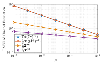
Figure 2: Error bounds for Eve’s channel estimation.

Perturbed by the proposed fake paths, the CRLB for Eve’s localization is presented in Figure 3 with different choices of $\bar{\delta}_{\tau}$ and $\bar{\delta}_{\theta_{\text{TX}}}$. According to Figure 3, coinciding with the analysis of the derived lower bounds, simultaneously decreasing the values of $\bar{\delta}_{\tau}$ and $\bar{\delta}_{\theta_{\text{TX}}}$ is desired to effectively degrade Eve’s localization accuracy. We note that, with the choices of $\bar{\delta}_{\tau}$ and $\bar{\delta}_{\theta_{\text{TX}}}$ in Figure 3, the assumptions A4 and A5 in Corollary 1 are not satisfied, suggesting that these sufficient conditions for the derivation of $\Psi^{(k)}$ are not necessary for the location-privacy enhancement.

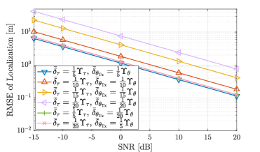
Figure 3: The influence of the choices of $\bar{\delta}_{\tau}$ and $\bar{\delta}_{\theta}$ on the $\sqrt{\text{CRLB}}$ for Eve’s localization.

VII-C Estimation Accuracy Comparison

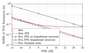
Figure 4: The $\sqrt{\text{CRLB}}$ for TOA estimation.

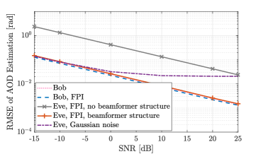
Figure 5: The $\sqrt{\text{CRLB}}$ for AOD estimation.

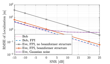
Figure 6: The $\sqrt{\text{CRLB}}$ for localization.

According to Sections V and VII-B, we assume $\delta_{\tau_{k},\min}=\frac{1}{20}\Upsilon_{\tau}$ and $\delta_{\theta_{\mathrm{Tx},{k}},\min}=\frac{1}{20}\Upsilon_{\theta}$ for any $k$ and we set $\bar{\delta}_{\tau}$ and $\bar{\delta}_{\theta_{\text{TX}}}$ to $\delta_{\tau_{k},\min}$ and $\delta_{\theta_{\mathrm{Tx},{k}},\min}$, respectively, to enhance the location-privacy. The RMSE of TOA estimation and AOD estimation is shown in Figures 4 and 5, respectively, where the CRLB for Bob’s estimation is compared with that for Eve’s estimation. As observed in Figures 4 and 5, without the leakage of the channel structure, our proposed scheme contributes to more than $25$dB degradation with respect to the TOA and AOD estimation, by virtue of the fact that the FPI effectively distorts the structure of Eve’s channel. In contrast, Bob can compensate for the presence of the fake paths given the secure side information.

Due to the strong degradation of the quality of channel estimates, a larger CRLB for Eve’s localization is achieved as seen in Figure 6. With respect to the localization accuracy, there is a $20$dB advantage for Bob versus Eve using our proposed scheme. As analyzed in Section VI-D, if the structure of Alice’s beamformer is unfortunately leaked to Eve, Eve can actively estimate the shared information $\bar{\bm{\delta}}$ to mitigate the perturbation of the fake paths while inferring Alice’s position so the efficacy of our scheme is degraded. However, considering the uncertainties in the shared information, there is still around $4$dB degradation of localization accuracy for Eve versus Bob according to Figure 6, indicating the robustness of our scheme with respect to the beamformer structure leakage. We note that the model order can be adjusted via changing the value of $\widetilde{K}$ at a certain rate such that Eve has insufficient samples to learn the true beamformer structure and has to tackle the virtually introduced fake paths. In addition, as shown in Figure 7, if we inject an additional set of fake paths, Eve’s localization accuracy can be further degraded at the cost of higher transmit power. On the other hand, more side information needs to be shared with Bob to maintain his performance. Hence, there is an interesting trade-off to be investigated in the future.

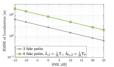
Figure 7: The $\sqrt{\text{CRLB}}$ for localization, 3 fake paths versus 6 fake paths, where $\bar{\delta}_{\tau}$ and $\bar{\delta}_{\theta_{\mathrm{Tx}}}$ are still set to $\frac{1}{20}\Upsilon_{\tau}$ and $\frac{1}{20}\Upsilon_{\theta}$ for the original 3 fake paths. With respect to the additionally injected 3 fake paths and the true paths, the separations for their TOAs and AODs are determined by the design parameters $\bar{\delta}_{\tau,2}$ and $\bar{\delta}_{\theta_{\mathrm{Tx}},2}$ that are set to $\frac{1}{10}\Upsilon_{\tau}$ and $\frac{1}{10}\Upsilon_{\theta}$, respectively.

To validate the efficacy of the FPI, CRLBs for channel estimation and localization with the injection of additional Gaussian noise [30] are also provided in Figures 4, 5 and 6 as comparisons. For relatively fair comparisons, the variance of the artificially added Gaussian noise $\widetilde{w}^{(g,n)}\sim\mathcal{CN}({0},\varsigma^{2})$ is set to a constant value for all the received SNRs, i.e., $\varsigma^{2}\triangleq\frac{\sum^{G}_{g=1}\sum^{N-1}_{n=0}\left|\widetilde{\bm{h}}^{(n)}{\boldsymbol{s}}^{(g,n)}\right|^{2}}{NG}$, while the received SNR is still defined as previously stated. As observed in Figures 4, 5 and 6, the injection of the extra Gaussian noise is ineffective to preserve location-privacy at low SNRs since its constant variance is relatively small as compared with that for the Gaussian noise naturally introduced during the transmission over the wireless channel. In contrast, through the degradation of the channel structure, the proposed FPI strongly enhances location-privacy. As the received SNR increases, the injection of the additional Gaussian noise can further degrade Eve’s performance due to the constant variance. However, the comparison is not fully fair as the amount of side information needed by Bob to remove the artificially injected Gaussian noise without CSI is high, i.e., the realization of $\widetilde{w}^{(g,n)}$ for all $g=1,2,\cdots,G$ and $n=0,1,\cdots,N-1$; our beamforming strategy requires very little side information, i.e., $\bar{\delta}_{\tau}$ and $\bar{\delta}_{\theta_{\text{TX}}}$. The exact amount of shared information transmitted over the secure channel depends on the distribution of the shared information required for the FPI, refresh rate, the quantization and coding strategy. The associated analysis is beyond the scope of this paper.

VIII Conclusions

A location-privacy enhancement strategy was investigated with the injection of fake paths. A novel CSI-free location-privacy enhancement framework was proposed, where the structure of the channel was exploited for the design of the fake paths. The injected fake paths were proved to be indistinguishable while two closed-form, lower bounds on the estimation error with the FPI were provided to validate that the proposed method can strongly degrade the eavesdropping ability of illegitimate devices. To effectively preserve location-privacy based on the proposed framework, a transmit beamformer was designed to inject the fake paths for the reduction of the LPL to illegitimate devices, while legitimate devices can maintain localization accuracy using the securely shared information. With respect to the CRLB for localization, there was $20$dB degradation in contrast to legitimate devices with the shared information and the robustness to the leakage of beamformer structure was also highlighted. Furthermore, the efficacy of the FPI was numerically verified with the comparison to unstructured Gaussian noise.

Appendix A Proof of Proposition 1

From the analysis for the feasibility of paths, to show Eve cannot make a distinction between fake paths and true paths, we seek to prove all the fake paths are geometrically feasible. To find the scatterers that can produce the injected fake paths, we consider $\widetilde{K}+1$ potential positions for these scatterers and denote by $b_{\widetilde{k}}$ the distance between Alice and the $\widetilde{k}$-th potential position, with $\widetilde{k}=0,1,\cdots,\widetilde{K}$. Then, the $\widetilde{k}$-th potential position, denoted as $\widetilde{\bm{v}}_{\widetilde{k}}=[\widetilde{v}_{{\widetilde{k}},x},\widetilde{v}_{{\widetilde{k}},y}]^{\mathrm{T}}\in\mathbb{R}^{2}$, can be mapped to $\{\widetilde{\tau}_{\widetilde{k}},\widetilde{\theta}_{\text{Tx},{\widetilde{k}}}\}$ according to Equation (3), i.e., the $\widetilde{k}$-th fake path is geometrically feasible, suppose that

• the inequality

  $$0\overset{\mathrm{(a)}}{\leq}b_{\widetilde{k}}\overset{\mathrm{(b)}}{\leq}c\widetilde{\tau}_{\widetilde{k}}\vspace{-3pt}$$ (34)

  holds;

• given $\widetilde{\theta}_{\text{Tx},{\widetilde{k}}}$, the equality

  $$\widetilde{\tau}_{\widetilde{k}}=\frac{b_{\widetilde{k}}+\left\|\left[\widetilde{v}_{{\widetilde{k}},x}-z_{x},\widetilde{v}_{{\widetilde{k}},y}-z_{y}\right]\right\|_{2}}{c},\vspace{-3pt}$$ (35)

  is satisfied, where $\left\|\left[\widetilde{v}_{{\widetilde{k}},x}-z_{x},\widetilde{v}_{{\widetilde{k}},y}-z_{y}\right]\right\|_{2}$ represents the distance between Eve and the $\widetilde{k}$-th potential position that can be expressed as

  $$\widetilde{v}_{{\widetilde{k}},x}= \ b_{\widetilde{k}}\cos(\widetilde{\theta}_{\text{Tx},{\widetilde{k}}})+p_{x},$$ (36a)

  $$\widetilde{v}_{{\widetilde{k}},y}= \ b_{\widetilde{k}}\sin(\widetilde{\theta}_{\text{Tx},{\widetilde{k}}})+p_{y}.\vspace{-3pt}$$ (36b)

According to Equation (35), we set the distance $b_{\widetilde{k}}$ to

$$b_{\widetilde{k}}=\frac{\left(c\widetilde{\tau}_{\widetilde{k}}\right)^{2}-\left(z_{x}-p_{x}\right)^{2}-\left(z_{y}-p_{y}\right)^{2}}{2\left(c\widetilde{\tau}_{\widetilde{k}}-\left(z_{x}-p_{x}\right)\cos(\widetilde{\theta}_{\text{Tx},{\widetilde{k}}})-\left(z_{y}-p_{y}\right)\sin(\widetilde{\theta}_{\text{Tx},{\widetilde{k}}})\right)}.\vspace{-3pt}$$ (37)

It can be verified that the condition C2) is satisfied using the distance $b_{\widetilde{k}}$ in Equation (37) if the condition C1) is met. Hence, the final step of this proof is to show Equation (34) holds if $b_{\widetilde{k}}$ is set according to Equation (37), under the assumption of $c\widetilde{\tau}_{\widetilde{k}}\geq\|\bm{z}-\bm{p}\|_{2}$.

For notational convenience, we introduce two variables $\dot{z}_{x}$ and $\dot{z}_{y}$ that are defined as $\dot{z}_{x}\triangleq z_{x}-p_{x}$ and $\dot{z}_{y}\triangleq z_{y}-p_{y}$. To prove $\mathrm{(a)}$, considering the assumption $c\widetilde{\tau}_{\widetilde{k}}\geq\|\bm{z}-\bm{p}\|_{2}>0$, we equivalently need to justify

$$c\widetilde{\tau}_{\widetilde{k}}-\dot{z}_{x}\cos(\widetilde{\theta}_{\text{Tx},{\widetilde{k}}})-\dot{z}_{y}\sin(\widetilde{\theta}_{\text{Tx},{\widetilde{k}}})\geq 0,\vspace{-3pt}$$ (38)

which holds since we have

$$\left(\dot{z}_{x}\cos(\widetilde{\theta}_{\text{Tx},{\widetilde{k}}})+\dot{z}_{y}\sin(\widetilde{\theta}_{\text{Tx},{\widetilde{k}}})\right)^{2}=$$ (39)

$$\dot{z}_{x}^{2}\cos^{2}(\widetilde{\theta}_{\text{Tx},{\widetilde{k}}})+\dot{z}_{y}^{2}\sin^{2}(\widetilde{\theta}_{\text{Tx},{\widetilde{k}}})+2\dot{z}_{x}\dot{z}_{y}\sin(\widetilde{\theta}_{\text{Tx},{\widetilde{k}}})\cos(\widetilde{\theta}_{\text{Tx},{\widetilde{k}}})$$

$$\overset{\mathrm{(c)}}{=}\dot{z}_{x}^{2}+\dot{z}_{y}^{2}-\left(\dot{z}_{x}\sin(\widetilde{\theta}_{\text{Tx},{\widetilde{k}}})-\dot{z}_{y}\cos(\widetilde{\theta}_{\text{Tx},{\widetilde{k}}})\right)^{2}$$

$$\leq\dot{z}_{x}^{2}+\dot{z}_{y}^{2}\overset{\mathrm{(d)}}{\leq}\left(c\widetilde{\tau}_{\widetilde{k}}\right)^{2}.\vspace{-3pt}$$

The equality $\mathrm{(c)}$ can be verified with the property of the trigonometric functions while inequality $\mathrm{(d)}$ holds according to the assumption $c\widetilde{\tau}_{\widetilde{k}}\geq\|\bm{z}-\bm{p}\|_{2}$. In addition, we can re-express $c\widetilde{\tau}_{\widetilde{k}}-b_{\widetilde{k}}$ as

$$\frac{\left(c\widetilde{\tau}_{\widetilde{k}}\right)^{2}+\dot{z}_{x}^{2}+\dot{z}_{y}^{2}-2c\widetilde{\tau}_{\widetilde{k}}\left(\dot{z}_{x}\cos(\widetilde{\theta}_{\text{Tx},{\widetilde{k}}})+\dot{z}_{y}\sin(\widetilde{\theta}_{\text{Tx},{\widetilde{k}}})\right)}{2\left(c\widetilde{\tau}_{\widetilde{k}}-\dot{z}_{x}\cos(\widetilde{\theta}_{\text{Tx},{\widetilde{k}}})-\dot{z}_{y}\sin(\widetilde{\theta}_{\text{Tx},{\widetilde{k}}})\right)},\vspace{-3pt}$$ (40)

where the denominator has been proved to be non-negative according to Equation (38). Hence, to validate $\mathrm{(b)}$, we need to prove that

$$\left(c\widetilde{\tau}_{\widetilde{k}}\right)^{2}+\dot{z}_{x}^{2}+\dot{z}_{y}^{2}-2c\widetilde{\tau}_{\widetilde{k}}\left(\dot{z}_{x}\cos(\widetilde{\theta}_{\text{Tx},{\widetilde{k}}})+\dot{z}_{y}\sin(\widetilde{\theta}_{\text{Tx},{\widetilde{k}}})\right)\geq 0.\vspace{-3pt}$$ (41)

Since we have

$$\left(2c\widetilde{\tau}_{\widetilde{k}}\left(\dot{z}_{x}\cos(\widetilde{\theta}_{\text{Tx},{\widetilde{k}}})+\dot{z}_{y}\sin(\widetilde{\theta}_{\text{Tx},{\widetilde{k}}})\right)\right)^{2}$$ (42)

$$\overset{\mathrm{(e)}}{\leq}4\left(c\widetilde{\tau}_{\widetilde{k}}\right)^{2}(\dot{z}_{x}^{2}+\dot{z}_{y}^{2})\leq\left(\left(c\widetilde{\tau}_{\widetilde{k}}\right)^{2}+\dot{z}_{x}^{2}+\dot{z}_{y}^{2}\right)^{2},$$

where $\mathrm{(e)}$ follows from Equation (39), Equation (41) holds, concluding the proof.

Appendix B Proof of Lemma 1

Proving Lemma 1 is equivalent to showing that each element of $\frac{1}{G}{\bm{J}}^{(\bm{\zeta}_{k})}$ converges a.s. to the corresponding element of $\breve{\bm{J}}^{(\bm{\zeta}_{k})}$ as $G\rightarrow\infty$. Therefore, according to their definitions with $\frac{\partial u^{(g,n)}}{\partial\bm{\bar{\tau}}[k]}$ and $\frac{\partial u^{(g,n)}}{\partial\bm{\bar{\theta}}_{\text{Tx}}[k]}$ presented in Equation (14), we restrict the derivations to

$$\frac{2}{G\sigma^{2}}\sum_{n=0}^{N-1}\sum_{g=1}^{G}\mathfrak{R}\left\{\left(\frac{\partial u^{(g,n)}}{\partial\bm{\bar{\tau}}[k]}\right)^{*}\frac{\partial u^{(g,n)}}{\partial\bm{\bar{\tau}}[k]}\right\}$$ (43)

$$\quad\quad\quad\quad\quad\quad\overset{\text{a.s.}}{\longrightarrow}\frac{8\pi^{2}O_{1}O_{6}}{(\sigma{NT_{s}})^{2}}|\bm{\bar{\gamma}}[k]|^{2},\text{ as }G\rightarrow\infty,$$

in Equation (B) as the others can be verified analogously, where $\mathrm{(f)}$ results from the law of large number.

$$\frac{2}{G\sigma^{2}}\sum_{n=0}^{N-1}\sum_{g=1}^{G}\mathfrak{R}\left\{\left(\frac{\partial u^{(g,n)}}{\partial\bm{\bar{\tau}}[k]}\right)^{*}\frac{\partial u^{(g,n)}}{\partial\bm{\bar{\tau}}[k]}\right\}$$

$$=\frac{2}{G\sigma^{2}}\sum_{n=0}^{N-1}\sum_{g=1}^{G}\mathfrak{R}\left\{\left(j\frac{2\pi\sqrt{N_{t}}n}{NT_{s}}\bar{\gamma}^{*}_{k}e^{j\frac{2\pi n\bar{\tau}_{k}}{NT_{s}}}\left(\bm{s}^{(g,n)}\right)^{\mathrm{H}}\bm{\alpha}(\bar{\theta}_{\text{Tx},k})\right)\left(-j\frac{2\pi\sqrt{N_{t}}n}{NT_{s}}\bar{\gamma}_{k}e^{-j\frac{2\pi n\bar{\tau}_{k}}{NT_{s}}}\bm{\alpha}(\bar{\theta}_{\text{Tx},k})^{\mathrm{H}}\bm{s}^{(g,n)}\right)\right\}$$

$$=\frac{2}{\sigma^{2}}\sum_{n=0}^{N-1}\mathfrak{R}\left\{\left(\frac{2\pi\sqrt{N_{t}}n}{NT_{s}}\right)^{2}|\bar{\gamma}_{k}|^{2}\bm{\alpha}(\bar{\theta}_{\text{Tx},k})^{\mathrm{H}}\left(\frac{1}{G}\sum_{g=1}^{G}\left(\bm{s}^{(g,n)}\right)\left(\bm{s}^{(g,n)}\right)^{\mathrm{H}}\right)\bm{\alpha}(\bar{\theta}_{\text{Tx},k})\right\}$$

$$\xrightarrow[\text{a.s.}]{\mathrm{(f)}}\frac{2}{\sigma^{2}}\sum_{n=0}^{N-1}\mathfrak{R}\left\{\left(\frac{2\pi n}{NT_{s}}\right)^{2}|\bar{\gamma}_{k}|^{2}\bm{\alpha}(\bar{\theta}_{\text{Tx},k})^{\mathrm{H}}\bm{\alpha}(\bar{\theta}_{\text{Tx},k})\right\}=\frac{2}{\sigma^{2}}\sum_{n=0}^{N-1}\left(\frac{2\pi n}{NT_{s}}\right)^{2}|\bm{\bar{\gamma}}[k]|^{2}=\frac{8\pi^{2}O_{1}O_{6}}{(\sigma{NT_{s}})^{2}}|\bm{\bar{\gamma}}[k]|^{2}.$$ (44)

Appendix C Proof of Proposition 3

For the $k$-th true path and the $k$-th fake path, considering the TOAs and AODs of the other paths as well as all the channel coefficients as the nuisance parameters, we can bound the mean squared error of $\widehat{\bm{\zeta}}^{(k)}$ as $\mathbb{E}\left\{\left(\widehat{\bm{\zeta}}^{(k)}-{\bm{\zeta}}^{(k)}\right)^{\mathrm{T}}\left(\widehat{\bm{\zeta}}^{(k)}-{\bm{\zeta}}^{(k)}\right)\right\}\geq\operatorname{Tr}\left({\left(\bm{J}^{(\bm{\zeta}_{k})}\right)^{-1}}\right)$ according to [26]. Following from Lemma 1, if $G\rightarrow\infty$, we have $G\operatorname{Tr}\left({\left(\bm{J}^{(\bm{\zeta}_{k})}\right)^{-1}}\right)\overset{\text{a.s.}}{\longrightarrow}\operatorname{Tr}\left({\left(\breve{\bm{J}}^{(\bm{\zeta}_{k})}\right)^{-1}}\right)$. Hence, for any real $\psi>0$, there always exists a positive integer $\mathcal{G}$ such that when $G\geq\mathcal{G}$, we have $G\operatorname{Tr}\left({\left(\bm{J}^{(\bm{\zeta}_{k})}\right)^{-1}}\right)>\operatorname{Tr}\left({\left(\breve{\bm{J}}^{(\bm{\zeta}_{k})}\right)^{-1}}\right)-\psi$ with probability of 1. Then, the final step is prove $\operatorname{Tr}\left({\left(\breve{\bm{J}}^{(\bm{\zeta}_{k})}\right)^{-1}}\right)\geq\Xi^{(k)}$.

Denoting by $\rho^{(k)}_{i}$ the $i$-th eigenvalue of $\breve{\bm{J}}^{(\bm{\zeta}_{k})}$ with $i=1,2,3,4$, we have the following lower bound on $\operatorname{Tr}\left({\left(\breve{\bm{J}}^{(\bm{\zeta}_{k})}\right)^{-1}}\right)$,

$$\operatorname{Tr}\left({\left(\breve{\bm{J}}^{(\bm{\zeta}_{k})}\right)^{-1}}\right)=\sum_{i=1}^{4}\frac{1}{\rho^{(k)}_{i}}\overset{\mathrm{(g)}}{\geq}\Xi^{(k)}\triangleq 4\sqrt[4]{\frac{1}{\prod_{i=1}^{4}\rho^{(k)}_{i}}},$$ (45)

where $\mathrm{(g)}$ follows from the inequality of arithmetic and geometric means. Then, leveraging Equation (18), the equality that $\prod_{i=1}^{4}\rho^{(k)}_{i}=\operatorname{det}\left(\breve{\bm{J}}^{(\bm{\zeta}_{k})}\right)$, and the assumption of $\delta_{\gamma_{k}}=\delta_{\gamma_{k},\min}=0$ yields the desired statement.

Appendix D Proof of Corollary 1

Under the assumption A1, the lower bound with $\Xi^{(k)}$ has been derived in Proposition 3. Given the assumptions A2 and A3, Equation (24) holds so we have the following inequalities,

$$2O_{1}O_{6}-\epsilon<\mathfrak{R}\left\{M_{1}^{(k)}M_{6}^{(k)}\right\}+O_{1}O_{6},$$ (46a)

$$2O_{4}O_{5}-\epsilon<\mathfrak{R}\left\{M_{4}^{(k)}M_{5}^{(k)}\right\}+O_{4}O_{5}$$ (46b)

$$\mathfrak{R}\left\{M_{2}^{(k)}M_{3}^{(k)}\right\}+O_{2}O_{3}<2O_{2}O_{3}+\epsilon.\vspace{-3pt}$$ (46c)

$$\left(\mathfrak{R}\left\{M_{1}^{(k)}M_{6}^{(k)}\right\}+O_{1}O_{6}\right)\left(\mathfrak{R}\left\{M_{4}^{(k)}M_{5}^{(k)}\right\}+O_{4}O_{5}\right)-\left(\mathfrak{R}\left\{M_{2}^{(k)}M_{3}^{(k)}\right\}+O_{2}O_{3}\right)^{2}$$ (47)

$$> \left(2O_{1}O_{6}-\epsilon\right)\left(2O_{4}O_{5}-\epsilon\right)-\left(2O_{2}O_{3}+\epsilon\right)^{2}=4\left(O_{1}O_{6}O_{4}O_{5}-\left(O_{2}O_{3}\right)^{2}\right)-2\epsilon(O_{1}O_{6}+2O_{2}O_{3}+O_{4}O_{5})=0.$$

With the definition of $\epsilon$, $\Xi^{(k)}_{1}$ in Equation (22) is a positive value according to Equation (47) so

$$\Xi^{(k)}_{1}\geq \frac{(NT_{s})^{4}}{\left(O_{1}O_{6}+\mathfrak{R}\left\{M_{1}M_{6}\right\}\right)\left(O_{4}O_{5}+\mathfrak{R}\left\{M_{4}M_{5}\right\}\right)}$$ (48)

$$\overset{\mathrm{(h)}}{\geq} \frac{(NT_{s})^{4}}{4O_{1}O_{4}O_{5}O_{6}}$$

holds, where $\mathrm{(h)}$ follows from Equation (20b). In addition, it can be verified that $\breve{\bm{J}}^{(\bm{\zeta}_{k})}$ is a positive semidefinite matrix so $\operatorname{det}\left(\breve{\bm{J}}^{(\bm{\zeta}_{k})}\right)\geq 0$ and thus $\Xi^{(k)}_{2}\geq 0$ according to Equation (47). Then, we have

$$\Xi^{(k)}_{2}\geq\frac{1}{\left(O_{1}O_{6}-\mathfrak{R}\left\{M_{1}M_{6}\right\}\right)\left(O_{4}O_{5}-\mathfrak{R}\left\{M_{4}M_{5}\right\}\right)},$$ (49)

where the denominator of the right-hand side can be bounded according to

$$O_{1}O_{6}-\mathfrak{R}\left\{M_{1}M_{6}\right\}$$ (50)

$$= \mathfrak{R}\left\{O_{1}O_{6}-M_{1}M_{6}\right\}$$

$$\leq |O_{1}O_{6}-M_{1}M_{6}|$$

$$= \left|\frac{1}{N_{t}}\sum_{n=0}^{N-1}\sum_{n_{t}=0}^{N_{t}-1}n^{2}\left(1-e^{j2\pi\left(\frac{n_{t}d\sin\left(\delta_{\theta_{\text{Tx},k}}\right)}{\lambda_{c}}-\frac{n\delta_{\tau_{k}}}{NT_{s}}\right)}\right)\right|$$

$$\overset{\mathrm{(i)}}{\leq} \frac{1}{N_{t}}\sum_{n=0}^{N-1}\sum_{n_{t}=0}^{N_{t}-1}n^{2}\left|\left(1-e^{j2\pi\left(\frac{n_{t}d\sin\left(\delta_{\theta_{\text{Tx},k}}\right)}{\lambda_{c}}-\frac{n\delta_{\tau_{k}}}{NT_{s}}\right)}\right)\right|$$

$$\overset{\mathrm{(j)}}{\leq} \frac{3\pi}{N_{t}}\sum_{n=0}^{N-1}\sum_{n_{t}=0}^{N_{t}-1}n^{2}\left|\frac{n_{t}d\sin\left(\delta_{\theta_{\text{Tx},k}}\right)}{\lambda_{c}}-\frac{n\delta_{\tau_{k}}}{NT_{s}}\right|$$

$$\overset{\mathrm{(k)}}{=} \frac{3\pi}{N_{t}}\sum_{n=0}^{N-1}\left(\frac{n^{3}\delta_{\tau_{k}}}{NT_{s}}+\sum_{n_{t}=1}^{N_{t}-1}n^{2}\left(\frac{n_{t}d\sin\left(\delta_{\theta_{\text{Tx},k}}\right)}{\lambda_{c}}-\frac{n\delta_{\tau_{k}}}{NT_{s}}\right)\right)$$

$$= \frac{\pi N(N-1)(2N-1)(N_{t}-1)d\sin\left(\delta_{\theta_{\text{Tx},k}}\right)}{4\lambda_{c}}$$

$$-\frac{3\pi N(N-1)^{2}(N_{t}-2)\delta_{\tau_{k}}}{4N_{t}T_{s}},\vspace{-5pt}$$

and

$$O_{4}O_{5}-\mathfrak{R}\left\{M_{4}M_{5}\right\}\leq \frac{3\pi NN_{t}(N_{t}-1)^{2}d\sin\left(\delta_{\theta_{\text{Tx},k}}\right)}{4\lambda_{c}}$$ (51)

$$-\frac{\pi(N_{t}-1)(2N_{t}-1)(N-1)\delta_{\tau_{k}}}{4T_{s}}.\vspace{-3pt}$$

Herein, it can be verified with some algebra that ${\mathrm{(i)}}$, ${\mathrm{(j)}}$, and ${\mathrm{(k)}}$ result from the triangle inequality, the assumption A4, and the assumption A5, respectively, while Equation (51) can be derived analogously. By leveraging Equations (49), (50) and (51), the quantity $\Xi^{(k)}_{2}$ can be further bounded as provided in Equation (52), where ${\mathrm{(l)}}$ follows from the fact that $N,N_{t}\geq 2$ holds for MISO OFDM systems. Then, substituting Equations (48) and (52) into Equation (22) simplifies $\Xi^{(k)}$ into $\aleph^{(k)}$ shown in Equation (53). Since the lower bound $\aleph^{(k)}$ holds for any $\delta_{\tau_{k}}$ and $\delta_{\theta_{\text{Tx},k}}$ that satisfy assumptions A1-A5, we can set $\delta_{\tau_{k}}=\frac{\sin\left(\delta_{\theta_{\mathrm{Tx},{k}}}\right)}{(N-1)\Lambda}$ for $\aleph^{(k)}$ so that Equation (23) can be verified with some algebra.

$$\Xi_{2}^{(k)}\geq \frac{4N_{t}T_{s}\Lambda}{\pi(N-1)\left((2N-1)(N_{t}-1)N_{t}\sin\left(\delta_{\theta_{\text{Tx},k}}\right)-3\Lambda N(N-1)(N_{t}-2)\delta_{\tau_{k}}\right)}$$ (52)

$$\times\frac{4T_{s}\Lambda}{\pi(N_{t}-1)\left(3N_{t}(N_{t}-1)\sin\left(\delta_{\theta_{\text{Tx},k}}\right)-\Lambda(2N_{t}-1)(N-1)\delta_{\tau_{k}}\right)}$$

$$\overset{\mathrm{(l)}}{\geq} \frac{(4T_{s}\Lambda)^{2}}{\pi^{2}N_{t}N^{2}\left((2N_{t}^{2}\sin\left(\delta_{\theta_{\text{Tx},k}}\right)-3\Lambda(N-1)(N_{t}-2)\delta_{\tau_{k}}\right)\left(3N_{t}\sin\left(\delta_{\theta_{\text{Tx},k}}\right)-\Lambda(N-1)\delta_{\tau_{k}}\right)}\vspace{-5pt}$$

$$\aleph^{(k)}= \frac{\lambda_{c}\sigma^{2}}{\sqrt{2}\pi^{\frac{5}{2}}d|\gamma_{k}|^{2}|\cos(\theta_{\text{Tx},k})\cos(\widetilde{\theta}_{\text{Tx},k})|}$$ (53)

$$\times\sqrt[4]{\frac{(N\Lambda)^{2}T_{s}^{6}}{O_{1}O_{4}O_{5}O_{6}N_{t}\left(2N_{t}^{2}\sin\left(\delta_{\theta_{\text{Tx},k}}\right)-3\Lambda(N-1)(N_{t}-2)\delta_{\tau_{k}}\right)\left(3N_{t}\sin\left(\delta_{\theta_{\text{Tx},k}}\right)-\Lambda(N-1)\delta_{\tau_{k}}\right)}}$$

Appendix E Proof of Proposition 4

Since we assume that Eve knows Alice’s beamformer structure, the associated noise-free observation is defined as

$$\iota^{(g,n)}\triangleq\sqrt{N_{t}}\sum_{k=0}^{K}{\gamma}_{k}e^{-j\frac{2\pi n{\tau}_{k}}{NT_{s}}}\bm{\alpha}({\theta}_{\text{Tx},k})^{\mathrm{H}}\widetilde{\bm{s}}^{(g,n)}.\vspace{-3pt}$$ (54)

Let $\varpi^{(g,n)}\triangleq\sqrt{N_{t}}\sum_{k=0}^{K}{\gamma}_{k}e^{-j\frac{2\pi n{\tau}_{k}}{NT_{s}}}\bm{\alpha}({\theta}_{\text{Tx},k})^{\mathrm{H}}{\bm{s}}^{(g,n)}$. It can be verified that $\iota^{(g,n)}\rightarrow 2\varpi^{(g,n)}$ as $\bar{\delta}_{\tau},\bar{\delta}_{\theta_{\mathrm{Tx}}}\rightarrow 0$. To derive the FIM for Eve’s channel estimation with the prior knowledge of the beamformer structure, we can compute the derivative $\frac{\partial\iota^{(g,n)}}{\partial\xi_{k}}$ by replacing ${\bm{s}}^{(g,n)}$ in Equation (14) with $\widetilde{\bm{s}}^{(g,n)}$, where $\xi_{k}\in\{\tau_{k},\theta_{\mathrm{Tx},k},\mathfrak{R}\{{\gamma_{k}}\},\mathfrak{I}\{{\gamma_{k}}\}\}$, while derive $\frac{\partial\iota^{(g,n)}}{\partial\bar{\delta}_{\tau}}$ and $\frac{\partial\iota^{(g,n)}}{\partial\bar{\delta}_{{\theta}_{\text{Tx}}}}$ as follows,

$$\frac{\partial\iota^{(g,n)}}{\partial\bar{\delta}_{\tau}} =-j\frac{2\pi{N_{t}}n}{NT_{s}}\sum_{k=0}^{K}{\gamma}_{k}e^{-j\frac{2\pi n\left({\tau}_{k}+\delta_{\tau}\right)}{NT_{s}}}{\bm{\alpha}({\theta}_{\text{Tx},k})^{\mathrm{H}}}$$

$$\quad\times\operatorname{diag}\left(\bm{\alpha}\left(\bar{\delta}_{\theta_{\text{Tx}}}\right)^{\mathrm{H}}\right)\bm{s}^{(g,n)},$$ (55a)

$$\frac{\partial\iota^{(g,n)}}{\partial\bar{\delta}_{{\theta}_{\text{Tx}}}} =j\frac{2\pi{N_{t}}d}{\lambda_{c}}\sum_{k=0}^{K}{\gamma}_{k}e^{-j\frac{2\pi n\left({\tau}_{k}+\delta_{\tau}\right)}{NT_{s}}}\cos(\bar{\delta}_{{\theta}_{\text{Tx}}})$$

$$\quad\times{\bm{\alpha}({\theta}_{\text{Tx},k})^{\mathrm{H}}}\operatorname{diag}([0,1,\cdots,N_{t}-1])$$

$$\quad\times\operatorname{diag}\left(\bm{\alpha}\left(\bar{\delta}_{\theta_{\text{Tx}}}\right)^{\mathrm{H}}\right)\bm{s}^{(g,n)}.\vspace{-5pt}$$ (55b)

Then, it is straightforward to show that, as $\bar{\delta}_{\tau},\bar{\delta}_{\theta_{\mathrm{Tx}}}\rightarrow 0$,

$$\frac{\partial\iota^{(g,n)}}{\partial\xi_{k}} \rightarrow 2\frac{\partial\varpi^{(g,n)}}{\partial\xi_{k}},$$ (56a)

$$\frac{\partial\iota^{(g,n)}}{\partial\bar{\delta}_{\tau}} \rightarrow\sum_{k=0}^{K}\frac{\partial\varpi^{(g,n)}}{\partial{\tau}_{k}},$$ (56b)

$$\frac{\partial\iota^{(g,n)}}{\partial\bar{\delta}_{\theta_{\text{Tx}}}} \rightarrow\sum_{k=0}^{K}\frac{\partial\varpi^{(g,n)}}{\partial{\theta}_{\text{Tx},k}}.\vspace{-5pt}$$ (56c)

On the other hand, similar to Equation (B), it can be verified that for any $\xi_{k}$ and $\xi_{k^{\prime}}\in\{\tau_{k^{\prime}},\theta_{\mathrm{Tx},k^{\prime}},\mathfrak{R}\{{\gamma_{k^{\prime}}}\},\mathfrak{I}\{{\gamma_{k^{\prime}}}\}\}$,

$$\frac{2}{\sigma^{2}}\sum_{n=0}^{N-1}\sum_{g=1}^{G}\mathfrak{R}\left\{\left(\frac{\partial\varpi^{(g,n)}}{\partial\xi_{k}}\right)^{*}\frac{\partial\varpi^{(g,n)}}{\partial\xi_{k^{\prime}}}\right\}\overset{\text{a.s.}}{\longrightarrow}0,\ k\neq{k^{\prime}},\vspace{-3pt}$$ (57)

holds when $G,N_{t}\rightarrow\infty$. Hence, given $\bar{\delta}_{\tau},\bar{\delta}_{\theta_{\mathrm{Tx}}}\rightarrow 0$ and $G,N_{t}\rightarrow\infty$, for any $\xi_{k}$, we have

$$2\bm{J}^{(\bm{\chi})}_{\bar{\delta}_{\tau},\xi_{k}}=2\bm{J}^{(\bm{\chi})}_{\xi_{k},\bar{\delta}_{\tau}} \rightarrow\bm{J}^{(\bm{\chi})}_{{\tau}_{k},\xi_{k}},$$ (58a)

$$2\bm{J}^{(\bm{\chi})}_{\bar{\delta}_{\theta_{\text{Tx}}},\xi_{k}}=2\bm{J}^{(\bm{\chi})}_{\xi_{k},\bar{\delta}_{\theta_{\text{Tx}}}} \rightarrow\bm{J}^{(\bm{\chi})}_{{\theta}_{\text{Tx},k},\xi_{k}},$$ (58b)

$$4\bm{J}^{(\bm{\chi})}_{\bar{\delta}_{\tau},\bar{\delta}_{\tau}} \rightarrow\sum_{k=0}^{K}\bm{J}^{(\bm{\chi})}_{{\tau}_{k},{\tau}_{k}},$$ (58c)

$$4\bm{J}^{(\bm{\chi})}_{\bar{\delta}_{\theta_{\text{Tx}}},\bar{\delta}_{\theta_{\text{Tx}}}} \rightarrow\sum_{k=0}^{K}\bm{J}^{(\bm{\chi})}_{{\theta}_{\text{Tx},k},{\theta}_{\text{Tx},k}},$$ (58d)

$$4\bm{J}^{(\bm{\chi})}_{\bar{\delta}_{\tau},\bar{\delta}_{\theta_{\text{Tx}}}}=4\bm{J}^{(\bm{\chi})}_{\bar{\delta}_{\theta_{\text{Tx}}},\bar{\delta}_{\tau}} \rightarrow\sum_{k=0}^{K}\bm{J}^{(\bm{\chi})}_{{\tau}_{k},{\theta}_{\text{Tx},k}}=\sum_{k=0}^{K}\bm{J}^{(\bm{\chi})}_{{\theta}_{\text{Tx},k},{\tau}_{k}}.\vspace{-3pt}$$ (58e)

Hence, two rows of $\bm{J}^{(\bm{\chi})}$ are linearly dependent on the other rows as $\bar{\delta}_{\tau},\bar{\delta}_{\theta_{\mathrm{Tx}}}\rightarrow 0$ and $G,N_{t}\rightarrow\infty$, i.e.,

$$2\left[\bm{J}^{(\bm{\chi})}_{\bar{\delta}_{\tau},\tau_{0}},\bm{J}^{(\bm{\chi})}_{\bar{\delta}_{\tau},\theta_{\text{Tx},0}},\cdots,\bm{J}^{(\bm{\chi})}_{\bar{\delta}_{\tau},\bar{\delta}_{\theta_{\text{Tx}}}}\right]$$

$$\rightarrow \sum_{k=0}^{K}\left[\bm{J}^{(\bm{\chi})}_{\tau_{k},\tau_{0}},\bm{J}^{(\bm{\chi})}_{\tau_{k},\theta_{\text{Tx},0}},\cdots,\bm{J}^{(\bm{\chi})}_{\tau_{k},\bar{\delta}_{\theta_{\text{Tx}}}}\right],$$ (59a)

$$2\left[\bm{J}^{(\bm{\chi})}_{\bar{\delta}_{\theta_{\text{Tx}}},\tau_{0}},\bm{J}^{(\bm{\chi})}_{\bar{\delta}_{\theta_{\text{Tx}}},\theta_{\text{Tx},0}},\cdots,\bm{J}^{(\bm{\chi})}_{\bar{\delta}_{\theta_{\text{Tx}}},\bar{\delta}_{\theta_{\text{Tx}}}}\right]$$

$$\rightarrow \sum_{k=0}^{K}\left[\bm{J}^{(\bm{\chi})}_{\theta_{\text{Tx},k},\tau_{0}},\bm{J}^{(\bm{\chi})}_{\theta_{\text{Tx},k},\theta_{\text{Tx},0}},\cdots,\bm{J}^{(\bm{\chi})}_{\theta_{\text{Tx},k},\bar{\delta}_{\theta_{\text{Tx}}}}\right],\vspace{-5pt}$$ (59b)

which leads to the desired statement.

References

• [1] Jianxiu Li and Urbashi Mitra “Channel State Information-Free Artificial Noise-Aided Location-Privacy Enhancement” In ICASSP 2023 - 2023 IEEE International Conference on Acoustics, Speech and Signal Processing (ICASSP), 2023, pp. 1–5 DOI: 10.1109/ICASSP49357.2023.10095571
• [2] Arash Shahmansoori et al. “Position and Orientation Estimation Through Millimeter-Wave MIMO in 5G Systems” In IEEE Transactions on Wireless Communications 17.3, 2018, pp. 1822–1835 DOI: 10.1109/TWC.2017.2785788
• [3] Bingpeng Zhou, An Liu and Vincent Lau “Successive Localization and Beamforming in 5G mmWave MIMO Communication Systems” In IEEE Transactions on Signal Processing 67.6, 2019, pp. 1620–1635 DOI: 10.1109/TSP.2019.2894789
• [4] Jianxiu Li, Maxime Ferreira Da Costa and Urbashi Mitra “Joint Localization and Orientation Estimation in Millimeter-Wave MIMO OFDM Systems via Atomic Norm Minimization” In IEEE Transactions on Signal Processing 70, 2022, pp. 4252–4264 DOI: 10.1109/TSP.2022.3198188
• [5] Roshan Ayyalasomayajula, Aditya Arun, Wei Sun and Dinesh Bharadia “Users Are Closer than They Appear: Protecting User Location from WiFi APs” In Proceedings of the 24th International Workshop on Mobile Computing Systems and Applications, HotMobile ’23 Newport Beach, California: Association for Computing Machinery, 2023, pp. 124–130 DOI: 10.1145/3572864.3580345
• [6] Ruiyun Yu et al. “A Location Cloaking Algorithm Based on Combinatorial Optimization for Location-Based Services in 5G Networks” In IEEE Access 4, 2016, pp. 6515–6527 DOI: 10.1109/ACCESS.2016.2607766
• [7] Stefano Tomasin and Javier German Luzon Hidalgo “Virtual Private Mobile Network with Multiple Gateways for B5G Location Privacy” In 2021 IEEE 94th Vehicular Technology Conference (VTC2021-Fall), Norman, OK, USA, 2021, pp. 1–6 DOI: 10.1109/VTC2021-Fall52928.2021.9625457
• [8] Paul Schmitt and Barath Raghavan “Pretty Good Phone Privacy” In 30th USENIX Security Symposium (USENIX Security 21) USENIX Association, 2021, pp. 1737–1754
• [9] Satashu Goel and Rohit Negi “Guaranteeing Secrecy using Artificial Noise” In IEEE Transactions on Wireless Communications 7.6, 2008, pp. 2180–2189 DOI: 10.1109/TWC.2008.060848
• [10] Stefano Tomasin “Beamforming and Artificial Noise for Cross-Layer Location Privacy of E-Health Cellular Devices” In 2022 IEEE International Conference on Communications Workshops (ICC Workshops), Seoul, Korea, Republic of, 2022, pp. 568–573 DOI: 10.1109/ICCWorkshops53468.2022.9814457
• [11] Javier Jiménez Checa and Stefano Tomasin “Location-Privacy-Preserving Technique for 5G mmWave Devices” In IEEE Communications Letters 24.12, 2020, pp. 2692–2695 DOI: 10.1109/LCOMM.2020.3018165
• [12] Sajjad Beygi, Amr Elnakeeb, Sunav Choudhary and Urbashi Mitra “Bilinear Matrix Factorization Methods for Time-Varying Narrowband Channel Estimation: Exploiting Sparsity and Rank” In IEEE Transactions on Signal Processing 66.22, 2018, pp. 6062–6075 DOI: 10.1109/TSP.2018.2872886
• [13] Amr Elnakeeb and Urbashi Mitra “Bilinear Channel Estimation for MIMO OFDM: Lower Bounds and Training Sequence Optimization” In IEEE Transactions on Signal Processing 69, 2021, pp. 1317–1331 DOI: 10.1109/TSP.2021.3056591
• [14] Jianxiu Li and Urbashi Mitra “Improved Atomic Norm Based Time-Varying Multipath Channel Estimation” In IEEE Transactions on Communications 69.9, 2021, pp. 6225–6235 DOI: 10.1109/TCOMM.2021.3087793
• [15] Javier Via “Robust secret key capacity for the MIMO induced source model” In 2014 IEEE International Conference on Acoustics, Speech and Signal Processing (ICASSP), Florence, Italy, 2014, pp. 8178–8182 DOI: 10.1109/ICASSP.2014.6855195
• [16] Rafael F. Schaefer, Ashish Khisti and H. Poor “Secure Broadcasting Using Independent Secret Keys” In IEEE Transactions on Communications 66.2, 2018, pp. 644–661 DOI: 10.1109/TCOMM.2017.2764892
• [17] Qiaosheng Zhang, Mayank Bakshi and Sidharth Jaggi “Covert Communication Over Adversarially Jammed Channels” In IEEE Transactions on Information Theory 67.9, 2021, pp. 6096–6121 DOI: 10.1109/TIT.2021.3096176
• [18] Uppalapati Somalatha and Parthajit Mohapatra “Role of Shared Key for Secure Communication Over 2-User Gaussian Z-Interference Channel” In IEEE Transactions on Information Forensics and Security 17, 2022, pp. 85–98 DOI: 10.1109/TIFS.2021.3132234
• [19] Ankur Moitra “Super-Resolution, Extremal Functions and the Condition Number of Vandermonde Matrices” In Proceedings of the Forty-Seventh Annual ACM Symposium on Theory of Computing, STOC ’15 Portland, Oregon, USA: Association for Computing Machinery, 2015, pp. 821–830 DOI: 10.1145/2746539.2746561
• [20] Weilin Li, Wenjing Liao and Albert Fannjiang “Super-Resolution Limit of the ESPRIT Algorithm” In IEEE Transactions on Information Theory 66.7, 2020, pp. 4593–4608 DOI: 10.1109/TIT.2020.2974174
• [21] Emmanuel J Candès and Carlos Fernandez-Granda “Towards a Mathematical Theory of Super-Resolution” In Communications on pure and applied Mathematics 67.6 Wiley Online Library, 2014, pp. 906–956
• [22] Qiuwei Li and Gongguo Tang “Approximate support recovery of atomic line spectral estimation: A tale of resolution and precision” In Applied and Computational Harmonic Analysis 48.3, 2020, pp. 891–948 DOI: https://doi.org/10.1016/j.acha.2018.09.005
• [23] Maxime Ferreira Da Costa and Urbashi Mitra “On the Stability of Super-Resolution and a Beurling–Selberg Type Extremal Problem” In 2022 IEEE International Symposium on Information Theory (ISIT), 2022, pp. 1737–1742 DOI: 10.1109/ISIT50566.2022.9834831
• [24] Alessio Fascista, Angelo Coluccia, Henk Wymeersch and Gonzalo Seco-Granados “Downlink Single-Snapshot Localization and Mapping With a Single-Antenna Receiver” In IEEE Transactions on Wireless Communications 20.7, 2021, pp. 4672–4684 DOI: 10.1109/TWC.2021.3061407
• [25] Gongguo Tang, Badri Narayan Bhaskar and Benjamin Recht “Near Minimax Line Spectral Estimation” In IEEE Transactions on Information Theory 61.1, 2015, pp. 499–512 DOI: 10.1109/TIT.2014.2368122
• [26] Louis L Scharf and Cédric Demeure “Statistical Signal Processing: Detection, Estimation, and Time Series Analysis” Prentice Hall, 1991
• [27] Zohair Abu-Shaban et al. “Error Bounds for Uplink and Downlink 3D Localization in 5G Millimeter Wave Systems” In IEEE Transactions on Wireless Communications 17.8, 2018, pp. 4939–4954 DOI: 10.1109/TWC.2018.2832134
• [28] Rico Mendrzik, Henk Wymeersch, Gerhard Bauch and Zohair Abu-Shaban “Harnessing NLOS Components for Position and Orientation Estimation in 5G Millimeter Wave MIMO” In IEEE Transactions on Wireless Communications 18.1, 2019, pp. 93–107 DOI: 10.1109/TWC.2018.2877615
• [29] Andrea Goldsmith “Wireless Communications” Cambridge University Press, 2005 DOI: 10.1017/CBO9780511841224
• [30] Jun Xu, Xiaodong Wang, Pengcheng Zhu and Xiaohu You “Privacy-Preserving Channel Estimation in Cell-Free Hybrid Massive MIMO Systems” In IEEE Transactions on Wireless Communications 20.6, 2021, pp. 3815–3830 DOI: 10.1109/TWC.2021.3053770