Differential Analysis of Triggers and Benign Features for Black-Box DNN Backdoor Detection

Abstract

This paper proposes a data-efficient detection method for deep neural networks against backdoor attacks under a black-box scenario. The proposed approach is motivated by the intuition that features corresponding to triggers have a higher influence in determining the backdoored network output than any other benign features. To quantitatively measure the effects of triggers and benign features on determining the backdoored network output, we introduce five metrics. To calculate the five-metric values for a given input, we first generate several synthetic samples by injecting the input’s partial contents into clean validation samples. Then, the five metrics are computed by using the output labels of the corresponding synthetic samples. One contribution of this work is the use of a tiny clean validation dataset. Having the computed five metrics, five novelty detectors are trained from the validation dataset. A meta novelty detector fuses the output of the five trained novelty detectors to generate a meta confidence score. During online testing, our method determines if online samples are poisoned or not via assessing their meta confidence scores output by the meta novelty detector. We show the efficacy of our methodology through a broad range of backdoor attacks, including ablation studies and comparison to existing approaches. Our methodology is promising since the proposed five metrics quantify the inherent differences between clean and poisoned samples. Additionally, our detection method can be incrementally improved by appending more metrics that may be proposed to address future advanced attacks.

I Introduction

Deep neural networks (DNN) should be secure and reliable since they are utilized in many applications [66, 67, 9, 22, 58, 56, 55, 14, 59, 57, 15]. Therefore, studying the security problems for DNN is an important research topic [3, 7, 20, 27, 32, 51, 23]. This paper considers defending against backdoor attacks in neural networks for classification tasks under a black-box scenario, in which only the network output is accessible and other information (e.g., model weights and intermediate layer outputs) is not available. Backdoor attacks may appear in models trained by a third party. In backdoor attacks, the attacker injects triggers into the network during the training phase. During the testing phase, the backdoored neural network outputs the attacker-chosen labels whenever the corresponding triggers appear. This paper proposes a novel defense against backdoor attacks based on a differential analysis of the behaviors of backdoor triggers and benign features used by the network for classification.

Although there is substantial literature on backdoor attacks and defenses, effective detection methods are scarce. Detecting backdoors is challenging due to the asymmetric-information advantage available to the adversary (i.e., the attacker has complete control of the trigger, whereas the defender has little information about the trigger). Among the existing defenses, many make assumptions about the trigger, such as assuming that the trigger is small or non-adaptive. However, the assumptions may not be valid in real-world situations because a clever attacker can design any trigger. Another set of existing literature assumes that the defender has access to a contaminated dataset that contains trigger information. In real-world cases, accessing a contaminated dataset may not be feasible for the defender. Some studies do not have assumptions on triggers or a need for contaminated datasets. However, they require a large amount of clean data. Collecting a large amount of clean data may not always be affordable to the defender. Many works focus on detecting if a neural network is backdoored and should be abandoned. However, this paper is interested in designing a detection algorithm with limited clean validation samples to reject poisoned inputs (i.e., the inputs with triggers) so that the backdoored model can still be used without causing considerable loss. Therefore, we propose a detection method that has no assumptions on triggers, does not require the availability of a contaminated dataset, and only requires a tiny clean validation dataset.

Our method is inspired by the definition of the backdoor attack: the attacker controls the neural network output by overriding the original logic of the network when he/she presents triggers. This overriding behavior of the neural network will be exposed only for poisoned inputs, whereas for clean inputs, the neural network behaves normally. Therefore, we claim that the trigger has a higher influence than the benign features in determining the backdoored network output. Based on this difference, we propose five metrics (i.e., robustness $r$, weakness $w$, sensitivity $s$, inverse sensitivity $is$, and noise invariance $Inv$) such that a function exists to separate the clean and poisoned inputs regarding their five-metric values.

To calculate the five-metric values for a given input, our detection algorithm generates a few synthetic images by injecting the input’s partial contents into samples from a tiny validation dataset and utilizes the output labels corresponding to the synthetic images. Having the computed five metrics, five novelty detectors are trained from the tiny validation dataset. The trained novelty detectors will output high (resp., low) confidence scores for clean (resp., poisoned) inputs because a clean (resp., poisoned) input’s metric values will be similar to (resp., different from) the clean validation samples’ metric values (i.e., the training data for the novelty detectors) with a high probability. Thereafter, a meta novelty detector fuses the confidence scores by the five trained novelty detectors. During online testing, our method determines if a new input is poisoned and should be rejected via assessing its meta confidence score output by the meta novelty detector.

Besides the backdoor study, the proposed five metrics also contribute to solving two important problems for hand-crafted features-based anomaly detection [13, 50, 36]: 1) designing an effective descriptor, and 2) deciding suitable features for specific anomaly detection situations [21]. Our approach is novel in that it contributes effective hand-crafted features for backdoor detection (which can be regarded as an anomaly detection) using the proposed five novel metrics and achieves high accuracy under a black-box scenario with scarce available clean samples, whereas existing hand-crafted features-based anomaly detection methods are not designed for backdoor detection purposes and hence are not as effective as ours.

Overall, the contributions of this paper include:

• We utilize the conceptual ways that triggers can be injected into a backdoored network in order to achieve an unsupervised approach for backdoor detection;

• We propose five metrics to measure the behavior of the network for different scenarios;

• We propose a data-efficient online detection algorithm using the five-metric values as inputs to detect poisoned inputs for neural networks under a black-box scenario;

• We evaluate and compare the efficacy of our detection approach with other methods on various backdoor attacks.

II Related Work

Backdoor attack was first proposed by [28] and [48]. Several types of backdooring triggers have been studied including triggers with semantic real-world meaning [71], hidden invisible triggers [43, 63, 42, 53], smooth triggers [76], and reflection triggers [49]. Backdoor attacks have been devised in several contexts including federated learning [74, 4, 2], transfer learning [75], graph networks [77], text-classification [16], and out-sourced cloud environments [26]. Several scenarios/variants of backdoor attacks have been considered including all-label attacks [28], clean label attacks [78, 46], and defense-aware attacks [45]. The backdooring mechanism has also been applied for benign/beneficial purposes, such as watermarking for patent protection [64].

Backdoor attack defenses can be classified into several groups regarding their assumptions or proposed methods. The reverse-engineering-based approaches [70, 62, 47, 29] attempt to solve an optimization problem under certain restrictive assumptions; hence, those methods are effective only in a small portion of cases. [18] proposed a gradient-free technology to reverse-engineer the trigger with limited data. Clustering-based approaches [68, 8, 73, 30] assume a contaminated training dataset is available, whose acquisition might be expensive. Novelty-detection-based approaches [40, 1, 54, 41, 10, 79] require enough clean validation samples for training the complex novelty detector models, especially for the neural-network-based novelty detectors. The retraining-based approaches [38, 23] also need a reasonable amount of clean data to achieve high performance. If the available clean data is not sufficient, their performance degrades dramatically. [24] used online data to improve detection accuracy. However, the method becomes ineffective when online data is limited. Some works tested if a network has a backdoor [34, 47] and should be abandoned. Fine-pruning [45] and STRIP [25] have their assumptions and limitations that require further improvements. Some works modify the original problem and show the behavior of the backdoored networks in their settings, such as noise response analysis [19] and generation of universal litmus patterns [35]. [76] studied backdoor attacks in the frequency domain.

III Problem Formulation

III-A Background and Assumptions

TABLE I: Behavior of benign and backdoored neural networks.

data / model	Benign $f$	Backdoored $f^{*}$
Clean $(z,l)$	$\mathbb{P}(f(z)=l)$ high	$\mathbb{P}(f^{*}(z)=l)$ high
Poisoned $(z^{*},l^{*})$	$\mathbb{P}(f(z^{*})=l)$ high	$\mathbb{P}(f^{*}(z^{*})=l^{*})$ high

The difference between a backdoored network and a benign network in classification is shown in Table I: a backdoored network $f^{*}$ outputs ground truth label $l$ for a clean input $z$ and a wrong label $l^{*}$ (called attacker-chosen label) for a poisoned input $z^{*}$ with a high probability, as shown in the last column in the table. However, poisoning an input adds negligible influence on the output of a benign model $f$, as shown in the middle column in the table.

We assume that only the network output is available to our approach. The network’s other information (e.g., gradients, weights, and hidden layer outputs) is not available. This black-box assumption makes our detection approach realistic since such internal access into the network may be unavailable due to proprietary/security considerations in real-world cases. Additionally, this black-box setting is widely used in the literature of neural network backdoor studies [18]. We assume that there is a small set of clean data $\{x_{i}\}_{i=1}^{n}$ (e.g., with size $n\leq 30$) to confirm the performance of $f$ on clean data. We assume that only the backdoor attack appears in our problem. Other types of attacks are out of the scope of this paper.

III-B Problem Formulation

Given a black-box network $f$ and a tiny validation dataset $\{x_{i}\}_{i=1}^{n}$, we want to find a detection algorithm $g(\cdot;\{x_{i}\}_{i=1}^{n},f)$ such that $g(z^{*};\{x_{i}\}_{i=1}^{n},f)=1$ with a high probability for poisoned inputs $z^{*}$ (if $f$ is backdoored) and $g(z;\{x_{i}\}_{i=1}^{n},f)=0$ with a high probability for clean inputs $z$, i.e.,

$$\mathbb{P}(g(z;\{x_{i}\}_{i=1}^{n},f)=0|z\text{ is clean}) \geq 1-\epsilon_{1},$$ (1)

$$\mathbb{P}(g(z^{*};\{x_{i}\}_{i=1}^{n},f)=1|z^{*}\text{ is poisoned}) \geq 1-\epsilon_{2}$$ (2)

where $\epsilon_{1}$ and $\epsilon_{2}$ are two small positive numbers.

III-C Important Concepts

Classification Accuracy (CA) is the ratio of the number of clean inputs for which the network outputs ground-truth labels to the total number of clean inputs. Both backdoored networks and benign networks should have high CA. Attack Success Rate (ASR) is the ratio of the number of poisoned inputs for which the network outputs attacker-chosen labels to the total number of poisoned inputs. ASR should be high for backdoored networks and low for benign networks.

True-Positive Rate (TPR) is the ratio of the number of poisoned inputs detected by the detection algorithm to the total number of poisoned inputs. An accurate detection algorithm should have high TPR. False-Positive Rate (FPR) is the ratio of the number of clean inputs misidentified as poisoned by the detection algorithm to the total number of clean inputs. An accurate detection algorithm should have low FPR.

Receiver Operating Characteristic Curve (ROC) is a graph that shows the detection algorithm’s performance at all thresholds. Its two parameters are TPR and FPR. Area Under the ROC Curve (AUROC) is the entire two-dimensional area underneath the entire ROC curve. An accurate detection algorithm should have AUROC close to 1. Area Under the Precision and Recall (AUPR) is similar to AUROC but with precision and recall as its two parameters. AUPR is useful when the testing dataset is imbalanced. Higher AUPR implies a better performance of the approach.

Novelty Detector is a one-class detector that learns the training data distribution and detects if an incoming new sample belongs to this distribution or not. In this paper, clean validation data and clean online data belong to the same distribution, whereas clean validation data and poisoned online data belong to different distributions.

IV Methodology

IV-A Intuition – Rethinking the Pattern-Based Triggers

Consider the naive trigger with functionality shown in Fig. 1: the trigger is one pixel with a fixed value located at the lower-right corner of the image. Any image attached with this trigger makes the backdoored network $f^{*}$ output the attacker-chosen label $l^{*}$ (i.e., 0). This shows that the trigger pattern has a higher influence than other benign features in deciding the network output. We measure this influence with the following steps: 1) given an image, we copy its partial content (i.e., the dashed area in Fig. 1) and paste the content into different clean validation samples in the exact corresponding location to generate synthetic images. 2) We feed these synthetic images into the network and observe the outputs. If the image is poisoned and the pasted content contains the trigger, then all the output labels should be $l^{*}$ (i.e., the left “Apply-Get” in Fig. 1). If the image is clean, it is less likely that all the output labels are the same (i.e., the right “Apply-Get” in Fig. 1). Therefore, the consistency among the network output labels for synthetic images can be used to measure this influence.

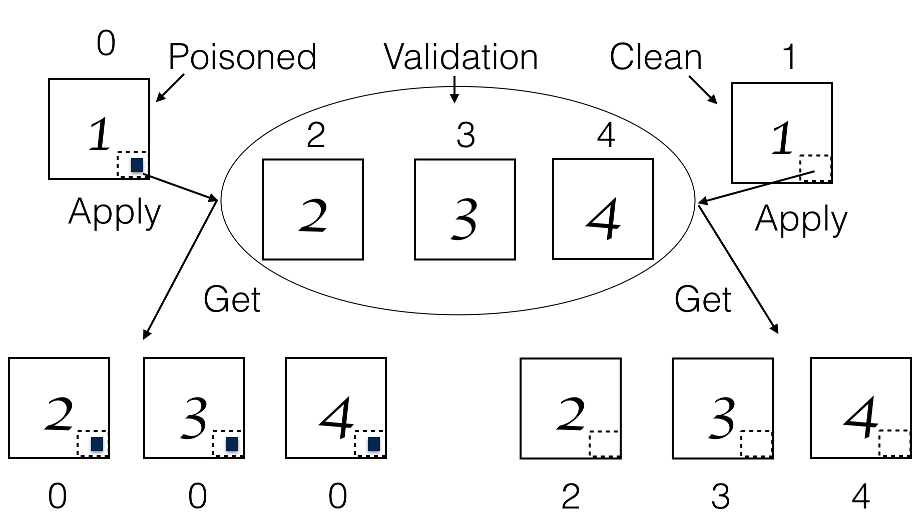
Figure 1: Network outputs before and after pasting the dashed area into the clean validation samples for the poisoned and clean input cases. The trigger is the black pixel. The attacker-chosen label is $0$. The number inside each image is the ground-truth label, whereas the number outside each image is the corresponding backdoored network output label.

Based on motivations analogous to the above discussion, we propose five metrics to quantitatively measure the effect of regions of a given image. Using these five metrics as a five-metric set, we will train a classifier that will enable testing of the given image for the presence of triggers.

IV-B The Five Metrics

The five proposed metrics are robustness $r$, weakness $w$, sensitivity $s$, inverse sensitivity $is$, and noise invariance $Inv$. Defining them will use the following notations:

• $z$ represents an input image to be evaluated for backdoor presence.

• $\{x_{i}\}_{i=1}^{n}$ represents $n$ clean validation samples.

• $U_{(\cdot)}$ represents the partial content of the image $(\cdot)$. For example, $U_{z}$ represents the partial content of image $z$.

• $paste(\cdot,*)$ pastes $(\cdot)$ into $(*)$ in the exact corresponding location and returns the synthetic image. For example, $paste(U_{z},x_{i})$ pastes $U_{z}$ into $x_{i}$ in the exact corresponding location and returns the synthetic image.

• $\mathds{1}$ represents the indicator function.

• $f^{*}$ represents the neural network (possibly backdoored).

• $\epsilon\sim\mathcal{N}(0,\delta)$ represents the normal noise tensor.

Robustness $r$ quantifies the likelihood that $U_{z}$ overrides the prediction of the backdoored network $f^{*}$ on $x_{i}$:

$$r=\frac{1}{n}\sum_{i=1}^{n}\mathds{1}\{f^{*}(z)=f^{*}(paste(U_{z},x_{i}))\}.$$ (3)

As one example scenario, if $z$ is poisoned and $U_{z}$ does not include the benign features of $z$ but includes the trigger, $r$ will be high. Inversely, if $z$ is clean and $U_{z}$ does not contain the benign features, $r$ will be low.

Weakness $w$ quantifies the likelihood that $U_{z}$ fails to make the backdoored network $f^{*}$ change its prediction on $x_{i}$:

$$w=\frac{1}{n}\sum_{i=1}^{n}\mathds{1}\{f^{*}(x_{i})=f^{*}(paste(U_{z},x_{i}))\}.$$ (4)

As one example scenario, if $z$ is poisoned and $U_{z}$ does not include the benign features of $z$ but includes the trigger, $w$ will be low. Inversely, if $z$ is clean and $U_{z}$ does not include the benign features, $w$ will be high.

Sensitivity $s$ quantifies the likelihood that $z$ still contains high influence features after $U_{x_{i}}$ is pasted:

$$s=\frac{1}{n}\sum_{i=1}^{n}\mathds{1}\{f^{*}(z)=f^{*}(paste(U_{x_{i}},z))\}.$$ (5)

As one example case, if $z$ is poisoned and $U_{x_{i}}$ contains the benign features of $x_{i}$ but $paste(U_{x_{i}},z)$ still contains the trigger, $s$ will be high. Inversely, if $z$ is clean and $U_{x_{i}}$ contains the benign features of $x_{i}$, $s$ will be low.

Inverse Sensitivity $is$ quantifies the likelihood that $z$ does not contain high influence features after $U_{x_{i}}$ is pasted:

$$is=\frac{1}{n}\sum_{i=1}^{n}\mathds{1}\{f^{*}(x_{i})=f^{*}(paste(U_{x_{i}},z))\}.$$ (6)

As one example scenario, if $z$ is poisoned and $U_{x_{i}}$ contains the benign features of $x_{i}$ but $paste(U_{x_{i}},z)$ still contains the trigger, $is$ will be low. Inversely, if $z$ is clean and $U_{x_{i}}$ contains the benign features of $x_{i}$, $is$ will be high. Thus, the metrics help distinguish between clean and poisoned samples.

The following observations are made:

• Each metric is expected to contribute in different ways to detect various triggers, although it is possible that multiple metrics capture the same trigger in some cases. Fusing all metrics further enhances the true positive rates and detection of the triggers. For example, one can easily design counterexamples for poisoned samples to evade detection using $r$ or $s$. However, $w$ and $is$ help complement $r$ and $s$ to detect those counterexamples.

• Having some reasonable regions $U$ is the key step to distinguishing the clean and poisoned samples. Therefore, we use several regions.

• These four metrics consider insertions of regions of a given image into corresponding regions of the validation set images (or vice versa), which are expected to be most relevant for pattern-based triggers (i.e., triggers contained in some regions in the image). However, non-pattern-based triggers exist (i.e., triggers that are based on inserting subtle variations throughout the image) and are usually entangled with benign features, which cannot be separated from benign features by any region. Consequently, the performance of these four metrics can be very low on certain non-pattern-based triggers. Therefore, the fifth metric $Inv$ is needed.

Noise Invariance $Inv$ quantifies the robustness of the features in $z$ against noise perturbation:

$$Inv=\frac{1}{n}\sum_{i=1}^{n}\mathds{1}\{f^{*}(z)=f^{*}(z+\epsilon_{i})\}.$$ (7)

If $z$ is poisoned and $\epsilon_{i}$ does not break the function of the benign features of $z$ but breaks the function of the trigger, $Inv$ will be low. Inversely, if $z$ is clean and $\epsilon_{i}$ does not break the function of the benign features, $Inv$ will be high. Thus, clean and poisoned samples are distinguishable. Similarly, finding the ideal noise $\epsilon$ is the key to distinguishing clean and poisoned samples. Therefore, we utilize a pool of noise distributions (i.e., different $\delta$). Fig. 2 is made with noise $\epsilon$ sampled from $\mathcal{N}(0,\delta)$ with different $\delta$ shown in the X-axis. The noise pattern is global with the same shape as the input image (i.e., a noise perturbation $\epsilon\sim\mathcal{N}(0,\delta)$ is added into each pixel of the image). From the figure, the clean and poisoned samples are empirically distinguishable. We also empirically observed that although $Inv$ is designed for non-pattern-based triggers, it also works well on some pattern-based triggers. The explanation is that some generated noise perturbations break the trigger pattern’s function but do not break the benign features’ influence. Overall, $Inv$ helps in distinguishing clean and poisoned samples, especially for non-pattern-based triggers and sometimes for pattern-based triggers.

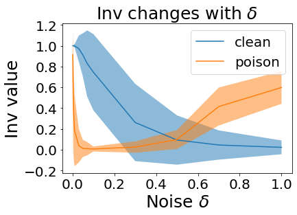
Figure 2: As noise variance $\delta$ changes, $Inv$ for the clean inputs decreases, whereas $Inv$ for the poisoned inputs decreases first and then increases. The plots show the average of multiple runs utilizing multiple samples in each run. The involved dataset is GTSRB [65] and the used trigger is Wanet [53].

IV-C The Pool of Feature Extraction Regions and Noise Variance

Separating different triggers and benign features could require multiple regions. Therefore, one should use a pool of regions to separate the triggers and benign features. Similarly, as shown in Fig. 2, a pool of $\delta$ can better capture the poisoned samples. This paper uses a pool of 16 central regions and a pool of 16 noise variances. Specifically, the aspect ratio of the central regions to the image is 0.1, 0.15, 0.2, 0.25, 0.3, 0.35, 0.4,0.45, 0.5,0.55, 0.6,0.65, 0.7,0.75, 0.8, and 0.9, respectively. And the noise variances are 0.001, 0.003, 0.005, 0.007, 0.01, 0.03, 0.05, 0.07, 0.1, 0.3, 0.5, 0.7, 1, 1.5, 2, and 3, respectively. Alg. 1 shows the extraction process used in this paper. We use the aspect ratio to calculate the coordinates of the extraction regions and then copy the content of the regions (i.e., $U_{z}$ and $U_{x_{i}}$) to calculate the five-metric values. Since the pool has 16 elements, each metric value will be a 16-dimensional vector. Note that the pools can be expanded by adding more regions and noise. For example, one can use and add extra regions with different locations and shapes. The paper later shows the performance of our approach using central regions and additional corner regions. Similarly, one can use and add extra noise perturbations from a wide range of distributions.

Algorithm 1 MetricCal($z$, $\{x_{i}\}_{i=1}^{n}$)

Initialization:

Ratio $\leftarrow$ [0.1, 0.15, 0.2, 0.25, 0.3, 0.35, 0.4,0.45, 0.5,0.55, 0.6,0.65, 0.7,0.75, 0.8, 0.9]

Variance $\leftarrow$ [0.001, 0.003, 0.005, 0.007, 0.01, 0.03, 0.05, 0.07, 0.1, 0.3, 0.5, 0.7, 1, 1.5, 2, 3]

### Calculating the Five-Metric Values for $z$ ###

H, W $\leftarrow$ Height of $z$, Width of $z$

$r,w,s,is,Inv\leftarrow\{\},\{\},\{\},\{\},\{\}$

for $j=1\to 16$ do

     k $\leftarrow$ Ratio[j]

     $m_{1},n_{1},m_{2},n_{2}\leftarrow\frac{1-k}{2}H,\frac{1-k}{2}W,\frac{1+k}{2}H,\frac{1+k}{2}W$

     $U_{z}\leftarrow z[m_{1}:m_{2},n_{1}:n_{2}]$

     $\{U_{x_{i}}\}_{i=1}^{n}\leftarrow\{x_{i}[m_{1}:m_{2},n_{1}:n_{2}]\}_{i=1}^{n}$

     $\delta\leftarrow$ Variance[j]

     $r_{j}^{\prime},w_{j}^{\prime},s_{j}^{\prime},is_{j}^{\prime},Inv_{j}^{\prime}\leftarrow$ (3), (4), (5), (6), (7)

     $r.append(r_{j}^{\prime})$, $w.append(w_{j}^{\prime})$

     $s.append(s_{j}^{\prime})$, $is.append(is_{j}^{\prime})$

     $Inv.append(Inv_{j}^{\prime})$

end for

Return: $r,w,s,is,Inv$

IV-D Novelty Detection Process

The novelty detection process is shown in Fig. 3. For any input $z$, we first calculate the five-metric values using the validation data, the pool of central regions, and the noise variances via $MetricCal$ in Alg. 1. The metric values are then sent into the corresponding novelty detectors, each of which will output a confidence score of the input not being a novelty. A meta novelty detector takes all five confidence scores to output a final confidence score. By setting a user-defined threshold, poisoned inputs can be detected. We expect each metric novelty detector to detect triggers in different ways. The reason to use the meta novelty detector is that it fuses the confidence scores nonlinearly and is more accurate than a simple linear combination of the confidence scores.

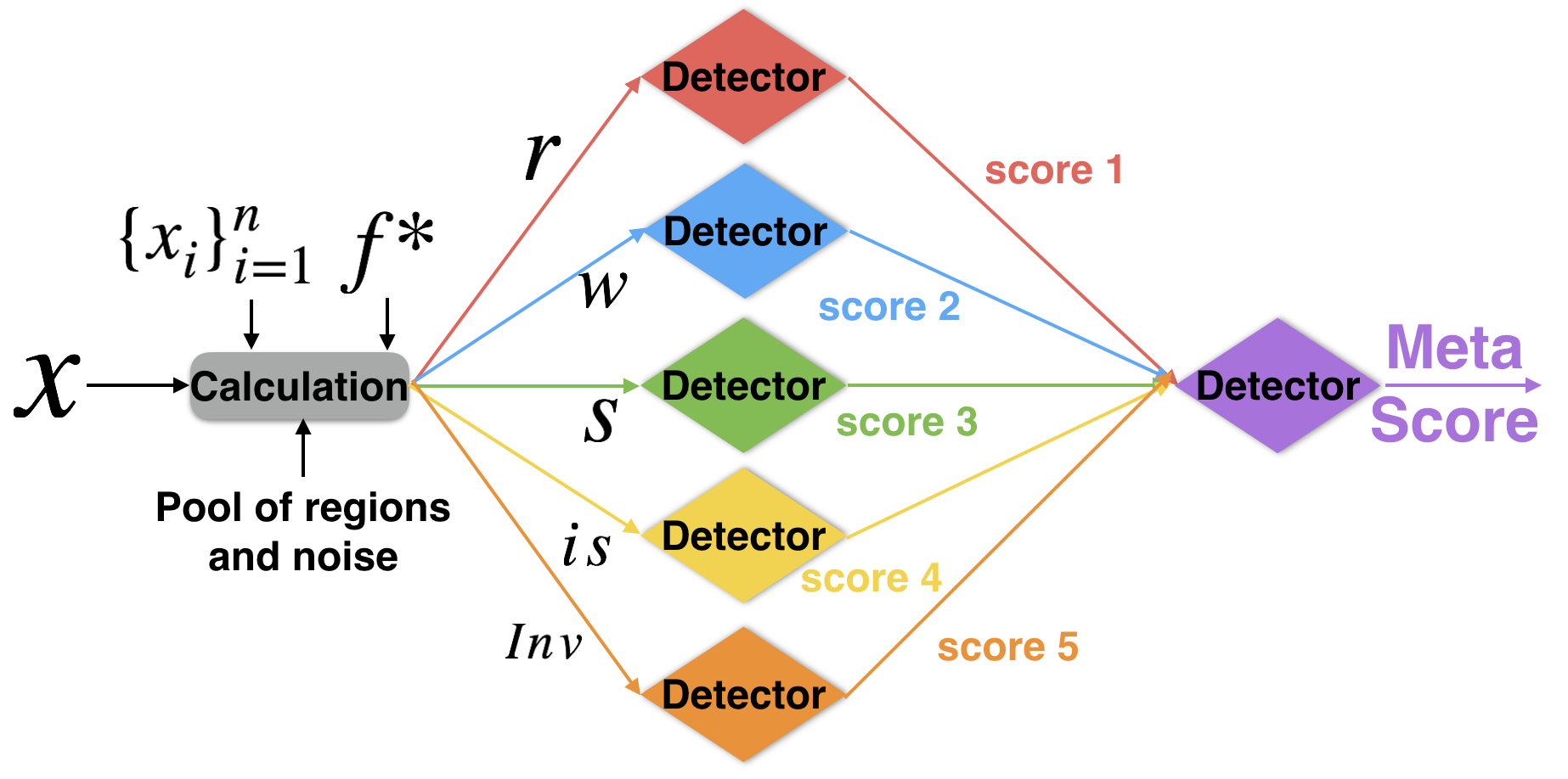
Figure 3: The novelty detection process: the five-metric values are first calculated for the input. Then each metric value is sent into a novelty detector that outputs a confidence score of the input not being a novelty. Lastly, five confidence scores are fed into a meta novelty detector to output a final confidence score.

In this paper, Local Outlier Factor (LOF) [6] from scikit-learn [60] with default parameter settings is used as the novelty detector. The meta novelty detector is also a LOF with default parameter settings. However, our approach is applicable to any type of anomaly detector and does not necessarily require nearest-neighbor detectors. Indeed, we empirically observed that our approach is also accurate with one-class SVM [12] as the novelty detector. The number of LOF’s parameters that need to be learned is small. Therefore, over-fitting is not likely to happen even if the available clean validation dataset is tiny. In contrast, novelty detectors with a large parameter size (e.g., neural-network-based detectors) are likely to face over-fitting with small training datasets. In this paper, the clean validation dataset size is $30$. Therefore, the neural-network-based novelty detectors may be over-fitted and have low accuracy. Training the LOF is simple: after the training data is prepared, one calls $model.fit$(training data) for training. We used default values set by scikit-learn for all the training hyper-parameters.

Algorithm 2 Detection Algorithm

Initialization:

Given validation dataset $\{x_{i}\}_{i=1}^{n}$ and network $f^{*}$

Off-line training:

### Calculating the Five-Metric Values for $\{x_{i}\}_{i=1}^{n}$ ###

$\{r_{l},w_{l},s_{l},is_{l},Inv_{l}\}_{l=1}^{n}\leftarrow\{MetricCal(x_{l},\{x_{i}\}_{i=1}^{n})\}_{l=1}^{n}$

### Training the First Set of Novelty Detectors ###

$\mathcal{N}_{r}.fit(\{r_{l}\}_{l=1}^{n})$, $\mathcal{N}_{w}.fit(\{w_{l}\}_{l=1}^{n})$, $\mathcal{N}_{s}.fit(\{s_{l}\}_{l=1}^{n})$

$\mathcal{N}_{is}.fit(\{is_{l}\}_{l=1}^{n})$, $\mathcal{N}_{Inv}.fit(\{Inv_{l}\}_{l=1}^{n})$

### Training the Meta Novelty Detector ###

$\{Score_{l}\}_{l=1}^{n}$ $\leftarrow$ $\{(\mathcal{N}_{r}.score(r_{l})$, $\mathcal{N}_{w}.score(w_{l})$, $\mathcal{N}_{s}.score(s_{l})$, $\mathcal{N}_{is}.score(is_{l})$, $\mathcal{N}_{Inv}.score(Inv_{l}))\}_{l=1}^{n}$

$\mathcal{N}_{meta}.fit(\{Score_{l}\}_{l=1}^{n})$

online detection:

Set a threshold $thres$

while True do

     Given an input $z$;

     $r,w,s,is,Inv\leftarrow MetricCal(z,\{x_{i}\}_{i=1}^{n})$

     $Score\leftarrow(\mathcal{N}_{r}.score(r),\mathcal{N}_{w}.score(w),\mathcal{N}_{s}.score(s)$,

     $\mathcal{N}_{is}.score(is),\mathcal{N}_{Inv}.score(Inv))$

     if $\mathcal{N}_{meta}.score(Score)<thres$ then

         $z$ is poisoned, and the output should not be trusted

     else

         $z$ is clean, and the output should be trusted

     end if

end while

IV-E The Detection Algorithm

Alg. 2 describes how to train the novelty detectors and use them to detect poisoned inputs. It first calculates the five-metric values for the clean validation samples $\{x_{i}\}_{i=1}^{n}$ using $MetricCal$ function. It then trains the five novelty detectors with the calculated metric values. The algorithm next feeds the calculated metric values to the trained novelty detectors to acquire the corresponding confidence scores. Finally, a meta novelty detector is trained with confidence scores. During online testing, the algorithm first calculates the metric values for a given input and then acquires the confidence scores by feeding the metric values into the first set of novelty detectors. It next feeds the scores into the meta novelty detector to get a meta score. If the meta score is lower than a user-defined threshold, the algorithm will consider $z$ poisoned. Otherwise, the input $z$ will be considered clean.

V Experimental Results

V-A Datasets, Triggers, and Compared Methods

TABLE II: Clean and poisoned samples per class in training and testing datasets and clean validation dataset Size.

		Train / Class		Test / Class		Total Valid
Dataset	Class	Clean	Poison	Clean	Poison	1st	2nd
MNIST	10	5500	825	1000	1000	30	100
GTSRB	43	820	123	294	294	30	100
CIFAR-10	10	5000	750	500	500	30	100
You. Face	1283	81	12	10	10	30	100
ImageNet	200	500	50	10	10	30	100

Clean Datasets and Network Architecture: Our method is evaluated on various datasets, including MNIST [39], GTSRB [65], CIFAR-10 [37], YouTube Face [72], and a subset of ImageNet [17]. The number of classes and the number of clean samples in the training and testing datasets for each class are shown in Table II. For MNIST, the model was from [28]. For GTSRB, the models were from [70] and Pre-activation Resnet-18 [31]. For CIFAR-10, the models were Network in Network [44] and Pre-activation Resnet-18. For YouTube Face, the network was from [70]. For ImageNet, Resnet-18 was used. Since our method addresses a black-box scenario, any backdoored models (even models other than neural networks, such as SVM [61] or random forest [5]) can be addressed.

Triggers and Their Impacts: The triggers for each dataset are shown in Fig. 4. In MNIST dataset, we considered all label attack (AAA) [28], clean label attack (CLA) [46], and blended (Ble.) [11]. Three additional triggers were created: the 4 corner trigger (4C) is four pixels at each corner; the 2 piece trigger (2P) is 2 pixels at the image’s center and upper-left corner; the centered trigger (Cen.) is one pixel located in the image center. The desired impact of the triggers is to misguide the backdoored network to output the attacker-chosen label $l^{*}$ given in Table III, where “+1” means $l^{*}=(l+1)$ mod 10. In CIFAR-10 dataset, we considered combination attack (TCA) [69] and Wanet (Wa.C) [53] with the impact shown in Table III. In GTSRB dataset, we considered a white box (Whi.) [70], a moving trigger (Mov.) [23, 69, 24], feature space attack (FSA) [47], and Wanet (Wa.G) [53]. In ImageNet dataset, we used an invisible (Invs.) trigger [43]. In YouTube Face dataset, we used sunglasses (Sun.) [11], lipstick (Lip.), and eyebrow (Eye.) [23, 69, 24] as triggers. All the impacts (i.e., $l^{*}$) can be found in Table III. This paper later discusses the trigger patterns in more detail.

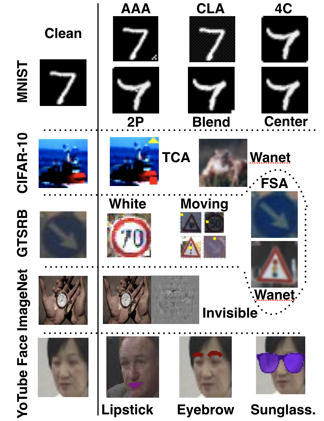
Figure 4: Clean and Poisoned Samples.

Details of Training Datasets: We randomly injected the corresponding triggers into 15% of the training clean samples for each class to create the training poisoned samples and changed the ground-truth label to the attacker-chosen label shown in Table III. Table II shows the number of clean and poisoned samples per class in the training dataset. CIFAR-10, YouTube Face, and Sub-Imagenet are balanced datasets. Therefore, the numbers in Table II are the numbers of samples per class in these three datasets. MNIST and GTSRB are not strictly balanced, but the numbers of samples per class for these two datasets are very close to the numbers shown in Table II. One can acquire more information on their distributions through the corresponding references. We followed the standard training process with CrossEntropy-based loss function and Adam optimizer to make the backdoored networks (badnet) have the classification accuracy (CA) and attack success rate (ASR) shown in Table III “Setup”.

TABLE III: Badnet behavior and accuracy, ablation study in ROC (unless specified), and performance of using the adaptive threshold.

Setup				Comparison, Different Regions, Replacing LOFs with OC-SVMs							Adaptive Threshold (%)
Badnet Behavior and Accuracy (%)				Ours		STRIP		Add Extra Reg.		OC-	Our Method		Applying
Trigger	$l^{*}$	CA	ASR	ROC	AUPR	ROC	AUPR	$\mathcal{N}_{w}$	Overall	SVM	TPR	FPR	CA	ASR
AAA	+1	97.24	95.17	0.938	0.974	0.457	0.601	0.972	0.972	0.972	100	7.6	90.7	0
CLA	0	89.1	100	0.934	0.972	0.914	0.915	0.781	0.971	0.969	100	8.31	87.09	0
4C	0	98.83	99.15	0.953	0.973	0.937	0.935	0.504	0.973	0.973	100	5.3	93.65	0
2P	0	99.17	94.71	0.965	0.973	0.959	0.962	0.524	0.972	0.962	94.1	1.35	97.93	1.1
Ble.	0	98.45	99.55	0.974	0.971	0.910	0.908	0.973	0.970	0.972	91.35	2.45	96.32	8.54
Cen.	0	98.96	92.21	0.989	0.974	0.782	0.778	0.972	0.972	0.972	92.6	1.05	98.04	3.01
Whi.	33	96.55	97.4	0.969	0.972	0.932	0.942	0.972	0.971	0.971	98.1	2.95	94.8	0.05
Mov.	0	95.15	99.88	0.988	0.973	0.845	0.854	0.707	0.973	0.972	99.75	1.01	94.62	0
FSA	35	95.03	90.2	0.930	0.935	0.402	0.423	0.777	0.928	0.940	90.2	4.9	91.34	0
TCA	7	88.9	99.7	0.965	0.973	0.967	0.970	0.485	0.973	0.970	95.45	1.85	87.65	4.27
Sun.	0	97.85	100	0.986	0.934	0.918	0.925	0.559	0.970	0.949	91.55	0.95	97.3	8.45
Lip.	0	97.3	91.39	0.962	0.957	0.881	0.898	0.732	0.947	0.946	88.7	0.83	96.81	2.85
Invs.	0	78.41	99.94	0.984	0.972	0.875	0.890	0.835	0.970	0.970	97.61	2.53	77.8	2.33
Wa.C	0	93.9	99.45	0.924	0.937	0.510	0.507	0.422	0.935	0.928	87.14	11.2	85.13	12.36
Wa.G	0	99.05	99.45	0.992	0.972	0.424	0.419	0.482	0.970	0.969	97.65	1.23	98.17	1.8

Details of Validation and Testing Datasets: Our work considers two small validation datasets with sizes $n=30$ and $100$ for all cases as shown in Table II. The first clean validation datasets were used for training all the novelty detectors. In this work, we randomly select clean samples to form the validation datasets so that the clean validation datasets have the same underlying data distributions as the clean testing datasets. We do not require the clean validation samples to be 100% correctly classified by the model. The number of samples per class for MNIST and YouTube Face is shown in the first row of Fig. 5. CIFAR-10 and MNIST have similar numbers of clean validation samples per class because they both have 10 classes, whereas the numbers of clean validation samples per class for GTSRB and sub-ImageNet are similar to YouTube Face because they all have a large number of classes. The second validation datasets were utilized to determine a proper threshold for our approach and have the same underlying distributions as the clean testing datasets as well. The second row in Fig. 5 shows the number of samples per class in the second clean validation datasets of MNIST and YouTube Face. Table II also shows the testing datasets that are used to evaluate our approach and other compared methods. The ratio of poisoned samples to clean samples is 1 (i.e., the testing datasets are balanced). Specifically, we generated the poisoned testing samples by injecting triggers into their corresponding clean versions. It is worth noticing that methods evaluated on imbalanced binary classification datasets may have high inference accuracy but poor run-time performance.

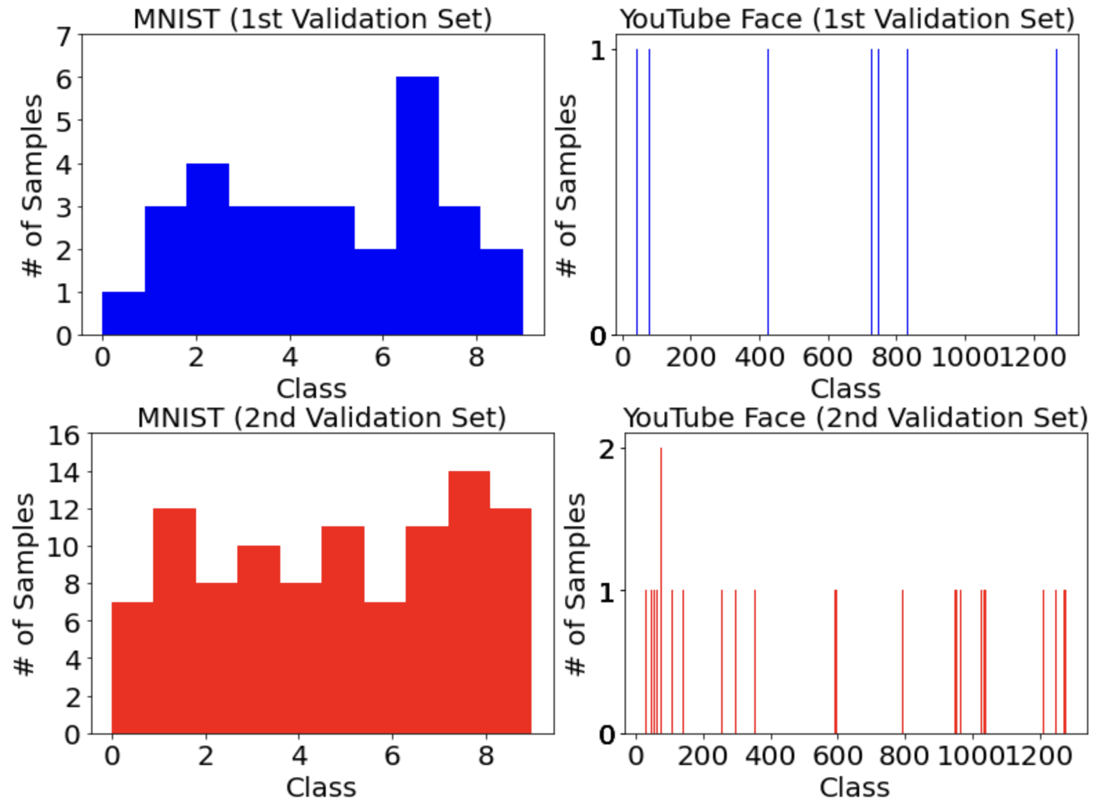
Figure 5: Histograms of clean validation datasets. Validation samples are randomly selected from the clean datasets. Blue: $n=30$. Red: $n=100$.

Compared Methods: We selected one reverse-engineering-based approach (i.e., Neural Cleanse [70]), one out-of-distribution detection (i.e., Mahalanobis-distance-based novelty detection (MD) [40]), one retraining-based approach (i.e., Kwon’s method [38]), and STRIP [25]. Neural Cleanse directly modifies the parameters of the original backdoored network to cap the maximum neuron values for the reverse-engineered triggers. Kwon’s method trains a new clean network on some relabeled poisoned samples. STRIP utilizes an entropy-based confidence score and “blend” technique for backdoor detection. MD is a feature-based anomaly detector with a Gaussian-based confidence score. MSP [33] and GEM [52] are two additional feature-based anomaly detectors whose performance was found to be close to MD. Therefore, for brevity, we only present the results with MD. The compared methods are representative in their types of defenses.

Fitting the Novelty Detectors: We used LOFs for the metric and meta novelty detectors. However, other types of novelty detectors are also allowed, such as one-class SVM. The training process is shown in Alg. 2. Only the clean validation datasets with size $n=30$ are available. Neither poisoned samples nor information about triggers were used. All the training hyper-parameters were set to default values provided by scikit-learn [60].

V-B Ablation Study for the Five Metrics

The ablation study shows the efficacy of each metric detector, the reasoning behind the validation dataset size and central regions, and improvement by incrementally adding metrics. The results are shown in Table III and Figs. 6-8.

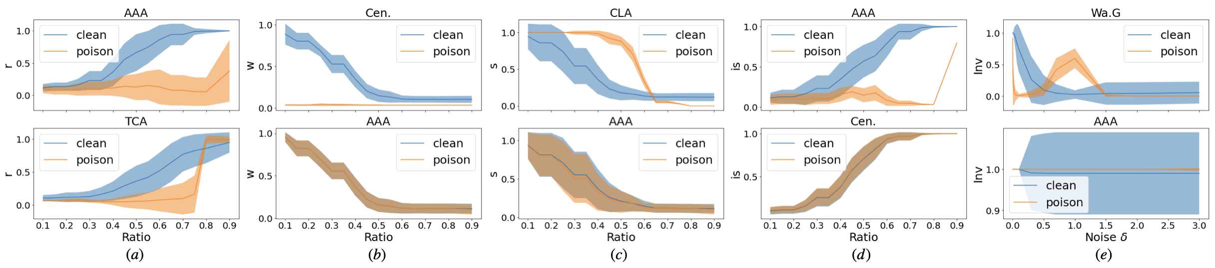
Figure 6: The five metrics values of clean and poisoned samples for different backdoor attack cases. The plots show the average of multiple runs utilizing multiple samples in each run. The first row shows the cases where clean and poisoned samples are distinguishable with respect to each metric value. The second row shows the cases where clean and poisoned samples are not distinguishable with respect to each metric value. (a): the visualization of (3) for $r$. (b): the visualization of (4) for $w$. (c): the visualization of (5) for $s$. (d): the visualization of (6) for $is$. (e) the visualization of (7) for $Inv$.

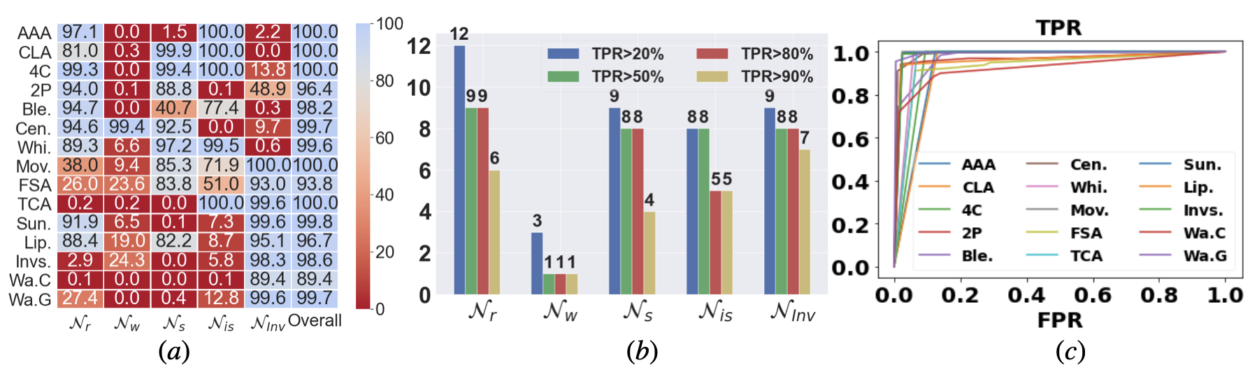
Figure 7: (a): TPR of the five metric novelty detectors. Overall: $or$ operation of the five novelty detectors. Higher numbers indicate better performance. (b): The total number of effective cases for each metric. (c): ROC curve for the meta novelty detector.

How Each Metric Works: To show the efficacy of the introduced five metrics given by (3), (4), (5), (6), and (7), we have plotted the five metrics values of clean and poisoned samples with respect to different aspect ratios (small ratios represent small central regions) and noise variances (small variances represent small noise perturbations) for several backdoor attack cases. The results are shown in Fig. 6. The first row shows the cases where clean and poisoned samples are distinguishable with respect to each metric value. Based on this observation, it is important to use several central regions with different sizes together to increase the detection probability of poisoned samples. For example, in the case AAA, clean and poisoned samples have similar $r$ and $is$ values for small central regions. However, they have distinguishable $r$ and $is$ values for large central regions. As for the case Cen., clean and poisoned samples are distinguishable in terms of $w$ for small and medium central regions. Clean and poisoned samples in CLA can be distinguished in terms of $s$ using medium central regions. Clean and poisoned samples in Wa.G can be distinguished by the metric $Inv$ using small and medium noise perturbations. The second row in Fig. 6 shows the cases where clean and poisoned samples are not distinguishable with respect to each metric value for all central regions and noise variances. Therefore, it is important to use all the five metrics together to increase the detection probability of poisoned samples. Details are given in the following ablation study.

Contribution of Each Metric: We calculated the five-metric values of the poisoned samples in the testing data for each backdoor attack case and input them into the five novelty detectors. After receiving the confidence scores, we calculated the TPR of each novelty detector using the default threshold value provided by scikit-learn (i.e., 0). Fig. 7(a) shows the TPR for each backdoor attack case. The “Overall” column is the final TPR of $or$ operation of the five novelty detectors. It is seen that each metric contributes to detecting poisoned inputs for some cases. Combining the five metrics can achieve a high TPR of over 90% for most cases except Wanet CIFAR-10 (Wa.C) whose TPR is 89.4%.

Fig. 7(b) shows the number of cases in which each metric contributes to detecting poisoned samples over the total 15 cases. $\mathcal{N}_{r}$ has a TPR of more than 20% in over 80% the cases. $\mathcal{N}_{w}$ helps increase the “Overall” TPR for some cases. For example, without using $\mathcal{N}_{w}$, the TPR reduces by 3% in both “Cen.” and “Lip.” cases. We also observed that $\mathcal{N}_{w}$ improved its own performance in some triggers if additional regions are utilized as shown in Table III “$\mathcal{N}_{w}$”. For more than half the cases, $\mathcal{N}_{s}$ and $\mathcal{N}_{is}$ have TPR of over 50%. Besides the non-pattern-based triggers, $\mathcal{N}_{Inv}$ is also effective on some pattern-based triggers since the generated noise breaks the impact of some pattern-based triggers, leading to an abrupt change in $Inv$ and the detection by $\mathcal{N}_{Inv}$.

The FPR of using the $or$ operation in “Overall” column is less than 30% for most cases. However, our meta novelty detector can reach a better trade-off between TPR and FPR than a simple $or$ operation of the five novelty detectors.

Performance of the Meta Novelty Detector: Choosing different threshold values $thres$ will lead to different TPR and FPR. We, therefore, draw the ROC curves for the meta novelty detector shown in Fig. 7(c) with the AUROC shown in Table III. The meta novelty detector can reach an AUROC over 0.9 for all the triggers. Therefore, for a proper threshold value, the meta novelty detector will have a high TPR and a low FPR. Although the testing datasets are balanced with an equal number of clean and poisoned samples, we still show the AUPR to investigate the performance of our approach in finding the poisoned samples. From Table III, our approach also has high AUPRs. Compared with the baseline method STRIP, our approach shows consistently high performance in all the cases, whereas STRIP performs poorly in several cases, such as AAA, Wa.C, and Wa.G. We also applied one-class SVM (OC-SVM) as the metric detectors and the meta detector and show the result in Table III. Based on the result, our approach is applicable to any type of anomaly detector and does not necessarily require LOFs.

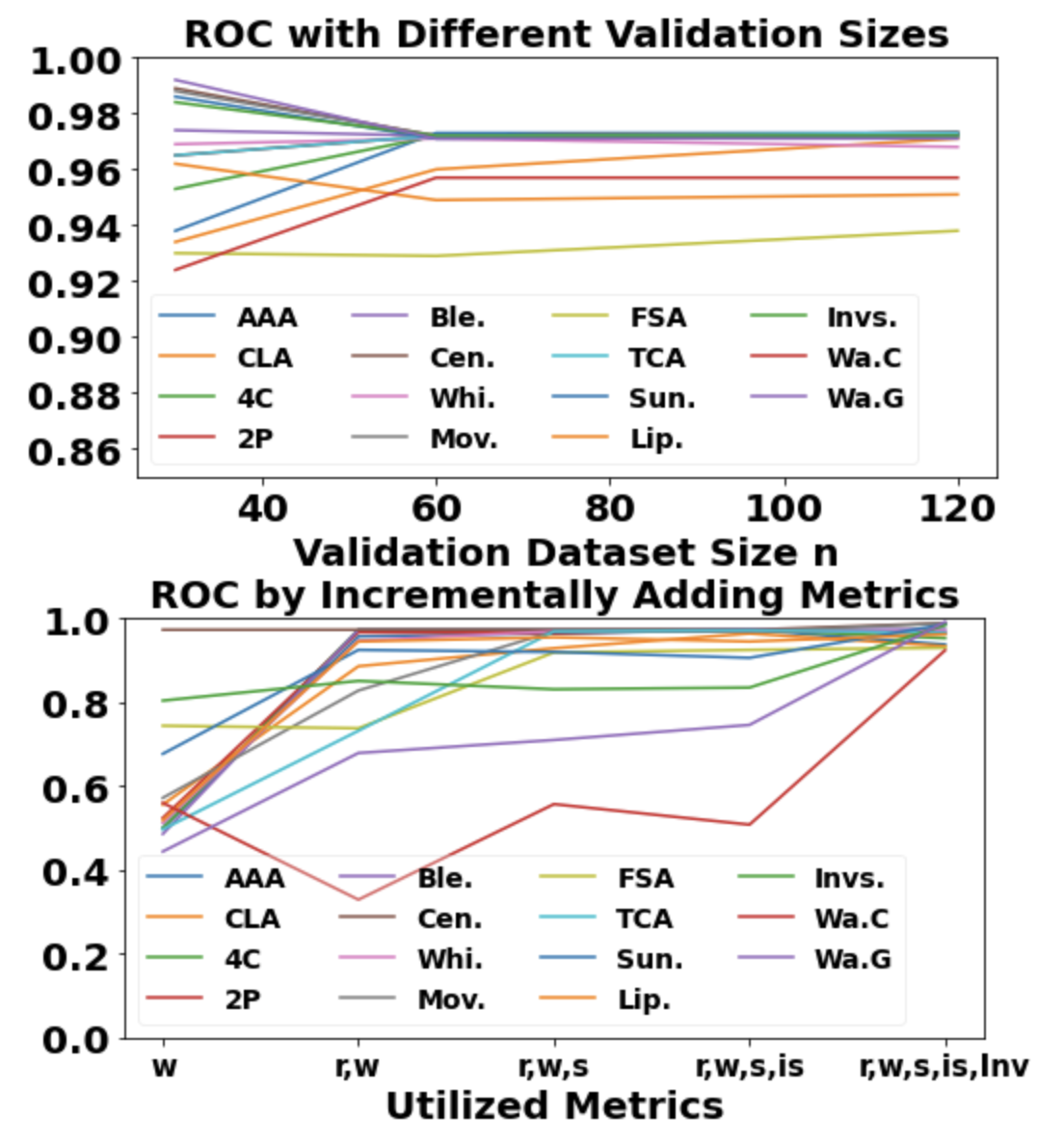
Figure 8: AUROC of the meta novelty detector with different clean validation dataset sizes $n$ (up) and incrementally adding metrics (bottom).

Regions, Sizes, and Incremental Improvements: We evaluated our approach by using additional regions. Specifically, the coordinates of the additional regions are $m_{1}=(1-k)L$, $n_{1}=(1-k)W$, $m_{2}=L$, and $n_{2}=W$, where $k$ is the aspect ratio from the same ratio pool in Alg. 1. The results are shown in Table III “Overall”. The AUROC of using extra regions is close to using only the central regions. Therefore, to minimize the computation cost, we choose to use only the central regions. The first plot in Fig. 8 shows the performance of our approach with different validation sizes. Using more validation samples does not significantly improve our approach but adds memory and computation complexity. Therefore, we consider $n=30$ to be optimal. The second plot in Fig. 8 shows the improvement of our approach by incrementally adding metrics. The AUROC is over 0.9 by using only two metrics ($w$ and $r$) in eight cases. With three metrics ($w$, $r$, and $is$), the AUROC is over 0.9 in twelve cases. Therefore, our approach requires metrics less than five to be accurate in some cases. Our approach in the remaining three cases requires all five metrics to achieve over 0.9 AUROC (using only $r$, $w$, $s$, and $is$, the AUROC of our approach is 0.835 for Invs., 0.508 for Wa.C, and 0.746 for Wa.G). To further highlight the contribution of each metric, we have evaluated our approach on all the cases by using only four metrics. The Sun. case mostly highlights the contribution of each metric. Therefore, this paper mainly discusses the Sun. case for brevity. The AUROC is 0.571 for using only $w$, $s$, $is$, $Inv$, 0.937 for using only $r$, $s$, $is$, $Inv$, 0.895 for using only $r$, $w$, $is$, $Inv$, 0.905 for using only $r$, $w$, $s$, $Inv$, and 0.906 for using only $r$, $w$, $s$, $is$. The AUROC of using all the five metrics is 0.986. According to these numbers, the metric $r$ contributes to detecting poisoned samples most for the Sun. case. However, the other four metrics also greatly fine-tune the performance of our approach by increasing the AUROC by roughly 5% $\sim$ 8%. Therefore, all the five metrics are needed to maximally capture poisoned samples.

V-C Adaptive Search for Threshold

Recall that our approach requires an appropriate threshold value is required to have a high TPR and a low FPR. To find such a threshold, we propose an adaptive-search solution. After the meta novelty detector is trained, one collects all the meta scores of the clean validation data (i.e., $\mathcal{N}_{meta}.score(\{Score_{l}\}_{l=1}^{n}$)). One finds the mean $\mu$ and standard deviation $\sigma$ of these meta scores. The threshold value can be set to $thres=\mu-h*\sigma$, where $h$ is a coefficient. With the second validation dataset available as shown in Table II, the user can vary $h$ and observe the FPR by testing the meta novelty detector on this validation dataset. Then, the user can choose the desired $h$ according to the corresponding FPR. If the second validation dataset is not available, the user can set $h$ to be any reasonable number.

With this adaptive search, our detection algorithm can reach the FPR of less than 5% and TPR of more than 90% for most cases, as shown in Table III. The CA and ASR of the backdoored network before and after applying our method are also shown in Table III. It is seen that our approach reduces the ASR by identifying and discarding potential poisoned inputs and maintains a reasonable CA. Even though our approach has a relatively low TPR (88.78%) for the trigger Lipsticks, the ASR for the Lipsticks is low (2.85%). This is because there exist null poisoned samples that fail to make the backdoored network output the attacker-chosen label. Since our approach is based on detecting differences in behaviors of the network when presented with triggers vs. benign features, the null poisoned samples may be considered clean by our approach and bypass the detection. However, failing to detect null poisoned samples does not increase the ASR. Note that the adaptive-search method can find better thresholds if a larger second validation dataset is used. For example, in Sun., the ASR can be further reduced to 0.9% with the CA being 95%.

V-D Data-Efficiency and Comparisons

TABLE IV: Original badnet performance and comparisons with compared methods on selected triggers and muti-trigger attacks.

	Bad Net.		Ours		Neural Cleanse [70]		MD [40]		Kwon’s [38]		STRIP [25]
Trigger	CA	ASR	CA	ASR	CA	ASR	CA	ASR	CA	ASR	CA	ASR
AAA	97.24	95.17	90.7	0	97.25	95.06	0	0	52.49	5.2	96.71	94.22
CLA	89.1	100	87.09	0	86.65	100	Fail		54.88	5.69	87.44	55.37
Whi.	96.55	97.4	94.8	0.05	96.55	97.44	Fail		25.45	0	96.03	97.13
Mov.	95.15	99.88	94.62	0	95.2	99.88	Fail		20.13	0	95.41	100
FSA	95.03	90.2	91.34	0	94.80	89.43	Fail		18.93	0	94.11	90.3
TCA	88.9	99.7	87.65	4.27	87.92	99.68	70.72	86.58	15.3	0	81.92	0.25
Sun.	97.85	100	97.3	8.45	97.59	99.90	Fail		1.1	0	90.74	7.02
Lip.	97.3	91.39	96.81	2.85	96.81	91.41	Fail		1.1	0	90.93	6.91
Sun., Lip., Eye. $l^{*}$	95.90	92.2	92.15	0	N/A	N/A	N/A	N/A	N/A	N/A	91	3.7
		92.2		0.5								41.7
		100		0								0
Sun., Lip., Eye. $l_{1}^{*},l_{2}^{*},l_{3}^{*}$	95.94	91.5	92.96	0.3	N/A	N/A	N/A	N/A	N/A	N/A	90.5	3.8
		91.3		0								32.3
		100		0								0
Invs.	78.41	99.94	77.8	2.33	N/A	N/A	0	0	N/A	N/A	74.01	24.13

We selected several types of triggers and compared our approach with other methods. We trained the baseline models with the two tiny validation datasets (i.e., a total of 130 samples) for a fair comparison. The hyper-parameters for training the compared methods were set based on the original papers and the codes provided by the authors. We set the thresholds for STRIP and MD so that 5% of the clean validation samples are considered poisoned. The results are summarized in Table IV.

Naive Triggers: The naive triggers (i.e., CLA and Whi.) are simple patterns associated with an attacker-chosen label. Our method reduces the ASR to a low value (maximum is 0.05%) while maintaining a reasonable CA. The other methods either do not work or cannot achieve comparable CA or ASR.

Functional Complex Triggers: According to the $l^{*}$ in Table III, the attack AAA depends on the trigger pattern and the image’s benign features. Additionally, AAA is a one-to-all attack with attacker-chosen label $l^{*}=l+1$ mod 10. The trigger of Mov. is randomly attached to the image. The trigger for TCA is the combination of two different shapes, and the network will output the attacker-chosen label only when both shapes exist. If only one shape appears in the image, the network behaves normally. The compared methods cannot both detect poisoned inputs and maintain high CA.

Real-World Meaning Triggers: The attacker uses some real-world objects as the triggers (i.e., Sun. and Lip.), and the trigger size can be large. Neural Cleanse cannot reverse-engineer large-sized triggers and thus has low accuracy. This is verified in Table IV. STRIP is still valid in this case, but our method shows a higher CA.

Filter Trigger and Invisible Sample-Specific Trigger: The trigger for FSA is a Gotham filter. Inputs that pass through this filter become poisoned. This trigger essentially changes the entire input image. However, our method shows its efficacy while all other methods fail. Trigger Invs. is an invisible sample-specific trigger. The attacker extracts content information and generates a hidden pattern for each image (the last picture in the “ImageNet” row in Fig. 4). By injecting the hidden pattern, the poisoned input looks identical to the clean input to human eyes (the middle picture in the “ImageNet” row), and the network will output the attacker-chosen label. Our method can detect this advanced attack as well.

Information Comparison: Table V shows the information needed for each method to detect or defend against backdoor attacks. For reverse-engineering-based approaches such as Neural Cleanse, they need access to the network parameters. However, it may not always be possible since such information could be proprietary. Feature-based statistical detection tools, such as MD, require some hidden layer outputs of the network. Compared to reverse-engineering-based approaches, they require less information about the network. Nevertheless, they may not be viable if the network is proprietary. The retraining-based approaches, such as Kwon’s, need the architecture of the network. However, to achieve high performance, they need a large amount of clean data, which may not be possible. Lastly, STRIP is a statistical detection tool that requires only the logits layer (i.e., the layer before the softmax function) output. However, if a neural network is entirely black-box, STRIP is also inapplicable. In contrast, our method can operate in completely black-box scenarios (black-box-efficient) and with smaller amounts of clean validation data (data-efficient).

TABLE V: Required information for each detection method.

Approach	Hidden Layer Output	Logits	Output Label
Ours	No	No	Required
Neural Cleanse	Required	Required	Required
MD	Required	No	No
Kwon’s	No	No	Required
STRIP	No	Required	No

Reasons for Low Accuracy on the Compared Methods: The most important reason for their low accuracy is that the available clean validation dataset is small. Neural Cleanse and Kwon’s method need to fine-tune a neural network model. The two tiny validation datasets are not enough to fine-tune neural network models to have high accuracy. MD and STRIP do not use neural networks. However, MD trains a novelty detector with hidden layer outputs of the validation samples, which are high-dimensional vectors (e.g., a 100-dimensional vector). The small number of validation samples and the high dimension of the hidden layer outputs make the trained novelty detector have low accuracy. STRIP uses the “blend” function to create synthetic images. However, there are many triggers whose functionality can be broken by the “blend” function. Therefore, STRIP becomes ineffective on those triggers. For example, STRIP is not accurate for one-to-all cases (i.e., AAA). Our method utilizes multiple regions to extract image contents to avoid breaking the triggers’ functionality.

V-E Benign Models and Multiple Triggers

Although our method does not detect if the model is backdoored and instead detects potentially poisoned inputs, other works (e.g., Neural Cleanse) can be used for checking if a model is backdoored. If the model is indeed backdoored, our method still applies to find poisoned inputs during online operation while using the model. If the model is clean but misidentified as backdoored, our method can retain a reasonable CA value. For example, we trained a benign model with MNIST dataset, which has 98.95% CA. After applying our method, the CA becomes 95.86%, which is still reasonable. Therefore, it is safe to use our method even when there are no backdoor attacks. We also considered multi-trigger-single-target attack (MTSTA) and multi-trigger-multi-target attack (MTMTA). In MTSTA, there are three triggers associated with a single attacker-chosen label. In MTMTA, the three triggers are associated with three different attacker-chosen labels. As shown in Table IV, our method works for both cases for all triggers. However, STRIP fails to detect some triggers.

VI Adaptive Attacks and Future Works

The proposed metrics help understand the backdoored network behavior. To bypass our detection, a backdoor attack needs to satisfy several conditions. Its trigger should be non-pattern-based since our approach uses four metrics to detect pattern-based triggers and attains high accuracy. Additionally, the robustness of the trigger against noise perturbation should be close to benign features so that the metric values $Inv$ for clean and poisoned samples are similar. The attacker can attempt to design an adaptive attack by using the five metrics in the training loss function. While we have not so far been able to devise a straightforward way to construct such an adaptive backdoor attack, it appears that the Wanet in CIFAR-10 case provides some clue in this direction since it provided a relatively low CA and high ASR compared to other attacks (although we did reasonably well in this case as well).

From the ablation studies, it appears that one metric $Inv$ is dominant for detecting non-pattern-based triggers although other metrics have some contribution. One potential direction for future work is to add new metrics for non-pattern-based triggers. For example, the denoising technique may also contribute to detecting non-pattern-based triggers. Another potential direction is to build new deep novelty detectors based on the existing ones to capture poisoned samples more accurately. The deep novelty detectors have shown promising performance for many applications. However, there are several factors that limit the existing deep novelty detectors to be utilized on detecting poisoned samples under the considered scenario. One factor is that training the deep novelty detectors requires sufficiently a large amount of data. Deep networks, such as LeNet, have thousands of parameters for even a single layer. However, the available clean samples considered in this work are scarce (i.e., $n\leq 30$). Therefore, the overfitting is likely to happen when using the existing deep novelty detectors for backdoor detection with limited data. Another factor is that the existing deep novelty detectors’ accuracy still requires improvement. Therefore, building new deep novelty detectors that are less demanding for data and more accurate for backdoor detection can be fruitful.

VII Conclusion

The behavioral differences between triggers and benign features are illustrated and utilized to detect backdoored networks. Five metrics are proposed to measure the behavior of the network for a given input. A novelty detection process is proposed to detect poisoned inputs by taking as input the five-metric values. The method is black-box-efficient and data-efficient. The ablation study for the five metrics, the efficacy of our approach, and the comparison with other methods are shown on various types of backdoor attacks. Potential adaptive attacks and prospective works are also discussed.

Hao Fu is a Ph.D. candidate in the Department of Electrical and Computer Engineering at New York University, Tandon School of Engineering, Brooklyn, NY, USA. In 2019, he received his M.S. degree in the same department. He received his B.S. in Physics from the University of Science and Technology of China, Hefei, China, in 2017. In 2018 Fall, he joined in Control/Robotics Research Laboratory (CRRL). His research interest is backdooring attacks and security in cyber-physical systems.

Prashanth Krishnamurthy received the B.Tech. degree in electrical engineering from Indian Institute of Technology Madras, Chennai, in 1999, and M.S. and Ph.D. degrees in electrical engineering from Polytechnic University (now NYU) in 2002 and 2006, respectively. He is a Research Scientist and Adjunct Faculty with the Department of Electrical and Computer Engineering at NYU Tandon School of Engineering. He has co-authored over 150 journal and conference papers and a book. His research interests include autonomous vehicles and robotic systems, multi-agent systems, sensor data fusion, robust and adaptive nonlinear control, resilient control, machine learning, real-time embedded systems, cyber-physical systems and cyber-security, decentralized and large-scale systems, and real-time software implementations.

Siddharth Garg received the B.Tech. degree in electrical engineering from the Indian Institute of Technology Madras, Chennai, India, and the Ph.D. degree in electrical and computer engineering from Carnegie Mellon University, Pittsburgh, PA, in 2009. He is currently an Associate Professor at New York University, New York, where he joined as an Assistant Professor in 2014. Prior to this, he was an Assistant Professor with the University of Waterloo, Waterloo, ON, Canada, from 2010 to 2014. His current research interests include computer engineering, and more particularly in secure, reliable, and energy efficient computing. He was a recipient of the NSF Career Award in 2015, and the paper awards at the IEEE Symposium on Security and Privacy 2016, the USENIX Security Symposium in 2013, the Semiconductor Research Consortium TECHCON in 2010, and the International Symposium on Quality in Electronic Design in 2009. He was listed in popular science magazine’s annual list of “Brilliant 10” researchers. He serves on the technical program committee of several top conferences in the area of computer engineering and computer hardware and has served as a reviewer for several IEEE and ACM journals conferences.

Farshad Khorrami received the bachelor’s degrees in mathematics and in electrical engineering from The Ohio State University in 1982 and 1984, respectively, and the master’s degree in mathematics and the Ph.D. degree in electrical engineering from The Ohio State University, in 1984 and 1988, respectively. He is currently a Professor with the Electrical and Computer Engineering Department, NYU, where he joined as an Assistant Professor in September 1988. He has developed and directed the Control/Robotics Research Laboratory, Polytechnic University (Now NYU) and Co-Director of the Center for AI and Robotics. His research has been supported by the DARPA, ARO, NSF, ONR, DOE, AFRL, NASA, and several corporations. He has published more than 320 refereed journal articles and conference papers in these areas. His book on ”modeling and adaptive nonlinear control of electric motors” was published by Springer Verlag in 2003. He also holds 14 U.S. patents on novel smart micropositioners and actuators, control systems, cyber security, and wireless sensors and actuators. His research interests include adaptive and nonlinear controls, robotics, unmanned vehicles (fixed-wing and rotary wing aircrafts as well as underwater vehicles and surface ships), machine learning, resilient control and cyber security for cyber-physical systems, large-scale systems, decentralized control, and real-time embedded instrumentation and control. He has served as the general chair and a conference organizing committee member for several international conferences.

References

- [1] Davide Abati, Angelo Porrello, Simone Calderara, and Rita Cucchiara. Latent space autoregression for novelty detection. In Proc. IEEE / CVF Comput. Vis. and Pattern Recog., pages 481–490, 2019.
- [2] Sebastien Andreina, Giorgia Azzurra Marson, Helen Möllering, and Ghassan Karame. Baffle: Backdoor detection via feedback-based federated learning. In Proc. Int. Conf. on Distrib. Comput. Syst., pages 852–863, 2021.
- [3] Anish Athalye, Nicholas Carlini, and David Wagner. Obfuscated gradients give a false sense of security: Circumventing defenses to adversarial examples. In Proc. Int. Conf. on Mach. Learn., pages 274–283, 2018.
- [4] Eugene Bagdasaryan, Andreas Veit, Yiqing Hua, Deborah Estrin, and Vitaly Shmatikov. How to backdoor federated learning. In Proc. Int. Conf. on Artif. Intell. and Statistics, pages 2938–2948, 2020.
- [5] Leo Breiman. Random forests. Mach. Learn., 45(1):5–32, 2001.
- [6] Markus M Breunig, Hans-Peter Kriegel, Raymond T Ng, and Jörg Sander. Lof: Identifying density-based local outliers. In Proc. ACM SIGMOD Int. Conf. on Management of Data, pages 93–104, 2000.
- [7] Nicholas Carlini and David Wagner. Towards evaluating the robustness of neural networks. In Proc. IEEE Symp. on Secur. and Privacy, pages 39–57, 2017.
- [8] Bryant Chen, Wilka Carvalho, Nathalie Baracaldo, Heiko Ludwig, Benjamin Edwards, Taesung Lee, Ian Molloy, and Biplav Srivastava. Detecting backdoor attacks on deep neural networks by activation clustering. In Proc. Workshop on Artif. Intell. Safety, 2019.
- [9] Chenyi Chen, Ari Seff, Alain Kornhauser, and Jianxiong Xiao. Deepdriving: Learning affordance for direct perception in autonomous driving. In Proc. Int. Conf. on Comput. Vis., pages 2722–2730, 2015.
- [10] Huili Chen, Cheng Fu, Jishen Zhao, and Farinaz Koushanfar. Deepinspect: A black-box trojan detection and mitigation framework for deep neural networks. In Proc. Int. Joint Conf. on Artif. Intell., pages 4658–4664, 2019.
- [11] Xinyun Chen, Chang Liu, Bo Li, Kimberly Lu, and Dawn Song. Targeted backdoor attacks on deep learning systems using data poisoning. arXiv preprint arXiv:1712.05526, 2017.
- [12] Yunqiang Chen, Xiang Sean Zhou, and Thomas S Huang. One-class svm for learning in image retrieval. In Proc. Int. Conf. on Image Process., volume 1, pages 34–37, 2001.
- [13] Yang Cong, Junsong Yuan, and Ji Liu. Sparse reconstruction cost for abnormal event detection. In Proc. IEEE / CVF Comput. Vis. and Pattern Recog., pages 3449–3456, 2011.
- [14] Bolun Dai, Prashanth Krishnamurthy, Andrew Papanicolaou, and Farshad Khorrami. State constrained stochastic optimal control using lstms. In Proc. Am. Control Conf., pages 1294–1299, 2021.
- [15] Bolun Dai, Prashanth Krishnamurthy, Andrew Papanicolaou, and Farshad Khorrami. State constrained stochastic optimal control for continuous and hybrid dynamical systems using dfbsde. Automatica, 155:111146, 2023.
- [16] Jiazhu Dai, Chuanshuai Chen, and Yufeng Li. A backdoor attack against lstm-based text classification systems. IEEE Access, 7:138872–138878, 2019.
- [17] J. Deng, W. Dong, R. Socher, L. Li, Kai Li, and Li Fei-Fei. Imagenet: A large-scale hierarchical image database. In Proc. IEEE / CVF Comput. Vis. and Pattern Recog., pages 248–255, 2009.
- [18] Yinpeng Dong, Xiao Yang, Zhijie Deng, Tianyu Pang, Zihao Xiao, Hang Su, and Jun Zhu. Black-box detection of backdoor attacks with limited information and data. In Proc. Int. Conf. on Comput. Vis., pages 16482–16491, 2021.
- [19] N Benjamin Erichson, Dane Taylor, Qixuan Wu, and Michael W Mahoney. Noise-response analysis of deep neural networks quantifies robustness and fingerprints structural malware. In Proc. SIAM Int. Conf. on Data Mining, pages 100–108, 2021.
- [20] Kevin Eykholt, Ivan Evtimov, Earlence Fernandes, Bo Li, Amir Rahmati, Chaowei Xiao, Atul Prakash, Tadayoshi Kohno, and Dawn Song. Robust physical-world attacks on deep learning visual classification. In Proc. IEEE / CVF Comput. Vis. and Pattern Recog., pages 1625–1634, 2018.
- [21] Yachuang Feng, Yuan Yuan, and Xiaoqiang Lu. Learning deep event models for crowd anomaly detection. Neurocomputing, 219:548–556, 2017.
- [22] Hao Fu, Prashanth Krishnamurthy, and Farshad Khorrami. Functional replicas of proprietary three-axis attitude sensors via LSTM neural networks. In Proc. IEEE Conf. on Control Technol. and Appl., pages 70–75, 2020.
- [23] Hao Fu, Akshaj Kumar Veldanda, Prashanth Krishnamurthy, Siddharth Garg, and Farshad Khorrami. Detecting backdoors in neural networks using novel feature-based anomaly detection. arXiv preprint arXiv:2011.02526, 2020.
- [24] Hao Fu, Akshaj Kumar Veldanda, Prashanth Krishnamurthy, Siddharth Garg, and Farshad Khorrami. A feature-based on-line detector to remove adversarial-backdoors by iterative demarcation. IEEE Access, 10:5545 – 5558, 2022.
- [25] Yansong Gao, Change Xu, Derui Wang, Shiping Chen, Damith C Ranasinghe, and Surya Nepal. Strip: A defence against trojan attacks on deep neural networks. In Proc. Annu. Comput. Secur. Appl. Conf., pages 113–125, 2019.
- [26] Xueluan Gong, Yanjiao Chen, Qian Wang, Huayang Huang, Lingshuo Meng, Chao Shen, and Qian Zhang. Defense-resistant backdoor attacks against deep neural networks in outsourced cloud environment. IEEE J. on Selected Areas in Commun., 39(8):2617–2631, 2021.
- [27] Ian J Goodfellow, Jonathon Shlens, and Christian Szegedy. Explaining and harnessing adversarial examples. In Proc. Int. Conf. on Learn. Representations, pages 1–14, 2015.
- [28] Tianyu Gu, Kang Liu, Brendan Dolan-Gavitt, and Siddharth Garg. Badnets: Evaluating backdooring attacks on deep neural networks. IEEE Access, 7:47230–47244, 2019.
- [29] Wenbo Guo, Lun Wang, Xinyu Xing, Min Du, and Dawn Song. Tabor: A highly accurate approach to inspecting and restoring trojan backdoors in AI systems. arXiv preprint arXiv:1908.01763, 2019.
- [30] Jonathan Hayase and Weihao Kong. Spectre: Defending against backdoor attacks using robust covariance estimation. In Proc. Int. Conf. on Mach. Learn., 2020.
- [31] Kaiming He, Xiangyu Zhang, Shaoqing Ren, and Jian Sun. Deep residual learning for image recognition. In Proc. IEEE / CVF Comput. Vis. and Pattern Recog., pages 770–778, 2016.
- [32] Warren He, James Wei, Xinyun Chen, Nicholas Carlini, and Dawn Song. Adversarial example defenses: Ensembles of weak defenses are not strong. In Proc. USENIX Workshop on Offensive Technol., pages 15–15, 2017.
- [33] Dan Hendrycks and Kevin Gimpel. A baseline for detecting misclassified and out-of-distribution examples in neural networks. In Proc. Int. Conf. on Learn. Representations, 2017.
- [34] Shanjiaoyang Huang, Weiqi Peng, Zhiwei Jia, and Zhuowen Tu. One-pixel signature: Characterizing cnn models for backdoor detection. In Proc. Eur. Conf. on Comput. Vis., pages 326–341, 2020.
- [35] Soheil Kolouri, Aniruddha Saha, Hamed Pirsiavash, and Heiko Hoffmann. Universal litmus patterns: Revealing backdoor attacks in cnns. In Proc. IEEE / CVF Comput. Vis. and Pattern Recog., pages 301–310, 2020.
- [36] Louis Kratz and Ko Nishino. Anomaly detection in extremely crowded scenes using spatio-temporal motion pattern models. In Proc. IEEE / CVF Comput. Vis. and Pattern Recog., pages 1446–1453, 2009.
- [37] Alex Krizhevsky and Geoffrey Hinton. Learning multiple layers of features from tiny images. Technical Report 0, University of Toronto, Toronto, Ontario, 2009.
- [38] Hyun Kwon. Detecting backdoor attacks via class difference in deep neural networks. IEEE Access, 8:191049–191056, 2020.
- [39] Yann LeCun and Corinna Cortes. MNIST handwritten digit database, 2010. http://yann.lecun.com/exdb/mnist.
- [40] Kimin Lee, Kibok Lee, Honglak Lee, and Jinwoo Shin. A simple unified framework for detecting out-of-distribution samples and adversarial attacks. In Proc. Advances in Neural Inf. Process. Syst., pages 7167–7177, 2018.
- [41] Kibok Lee, Kimin Lee, Kyle Min, Yuting Zhang, Jinwoo Shin, and Honglak Lee. Hierarchical novelty detection for visual object recognition. In Proc. IEEE / CVF Comput. Vis. and Pattern Recog., pages 1034–1042, 2018.
- [42] Shaofeng Li, Minhui Xue, Benjamin Zhao, Haojin Zhu, and Xinpeng Zhang. Invisible backdoor attacks on deep neural networks via steganography and regularization. IEEE Trans. on Dependable and Secure Comput., 2020.
- [43] Yuezun Li, Yiming Li, Baoyuan Wu, Longkang Li, Ran He, and Siwei Lyu. Invisible backdoor attack with sample-specific triggers. In Proc. Int. Conf. on Comput. Vis., pages 16463–16472, 2021.
- [44] Min Lin, Qiang Chen, and Shuicheng Yan. Network in network. In Proc. Int. Conf. on Learn. Representations, pages 1–10, 2014.
- [45] Kang Liu, Brendan Dolan-Gavitt, and Siddharth Garg. Fine-pruning: Defending against backdooring attacks on deep neural networks. In Proc. Int. Symp. on Res. in Attacks, Intrusions, and Defenses, pages 273–294, 2018.
- [46] Kang Liu, Benjamin Tan, Ramesh Karri, and Siddharth Garg. Poisoning the (data) well in ml-based cad: A case study of hiding lithographic hotspots. In Proc. Design, Autom. & Test in Eur. Conf. & Exhib., pages 306–309, 2020.
- [47] Yingqi Liu, Wen-Chuan Lee, Guanhong Tao, Shiqing Ma, Yousra Aafer, and Xiangyu Zhang. Abs: Scanning neural networks for back-doors by artificial brain stimulation. In Proc. ACM SIGSAC Conf. on Comput. and Commun. Secur., pages 1265–1282, 2019.
- [48] Yingqi Liu, Shiqing Ma, Yousra Aafer, Wen-Chuan Lee, Juan Zhai, Weihang Wang, and Xiangyu Zhang. Trojaning attack on neural networks. In Proc. Annu. Network And Distrib. Syst. Secur. Symp., 2018.
- [49] Yunfei Liu, Xingjun Ma, James Bailey, and Feng Lu. Reflection backdoor: A natural backdoor attack on deep neural networks. In Proc. Eur. Conf. on Comput. Vis., pages 182–199, 2020.
- [50] Ramin Mehran, Alexis Oyama, and Mubarak Shah. Abnormal crowd behavior detection using social force model. In Proc. IEEE / CVF Comput. Vis. and Pattern Recog., pages 935–942, 2009.
- [51] Seyed-Mohsen Moosavi-Dezfooli, Alhussein Fawzi, Omar Fawzi, and Pascal Frossard. Universal adversarial perturbations. In Proc. IEEE / CVF Comput. Vis. and Pattern Recog., pages 1765–1773, 2017.
- [52] Peyman Morteza and Yixuan Li. Provable guarantees for understanding out-of-distribution detection. In Proc. AAAI Conf. on Artif. Intell., volume 8, 2022.
- [53] Tuan Anh Nguyen and Anh Tuan Tran. Wanet - imperceptible warping-based backdoor attack. In Proc. Int. Conf. on Learn. Representations, 2021.
- [54] Poojan Oza, Hien V Nguyen, and Vishal M Patel. Multiple class novelty detection under data distribution shift. In Proc. Eur. Conf. on Comput. Vis., pages 432–449, 2020.
- [55] Naman Patel, Anna Choromanska, Prashanth Krishnamurthy, and Farshad Khorrami. A deep learning gated architecture for UGV navigation robust to sensor failures. Robot. and Auton. Syst., 116:80–97, 2019.
- [56] Naman Patel, Prashanth Krishnamurthy, Siddharth Garg, and Farshad Khorrami. Adaptive adversarial videos on roadside billboards: Dynamically modifying trajectories of autonomous vehicles. In Proc. IEEE/RSJ Int. Conf. on Intell. Robots and Syst., pages 5916–5921, 2019.
- [57] Naman Patel, Prashanth Krishnamurthy, Siddharth Garg, and Farshad Khorrami. Overriding autonomous driving systems using adaptive adversarial billboards. IEEE Trans. on Intell. Transportation Syst., 23(8):11386–11396, 2021.
- [58] Naman Patel, Apoorva Nandini Saridena, Anna Choromanska, Prashanth Krishnamurthy, and Farshad Khorrami. Adversarial learning-based on-line anomaly monitoring for assured autonomy. In Proc. IEEE/RSJ Int. Conf. on Intell. Robots and Syst., pages 6149–6154, 2018.
- [59] Naman Patel, Apoorva Nandini Saridena, Anna Choromanska, Prashanth Krishnamurthy, and Farshad Khorrami. Learning-based real-time process-aware anomaly monitoring for assured autonomy. IEEE Trans. on Intell. Vehicles, 5(4):659–669, 2020.
- [60] F. Pedregosa, G. Varoquaux, A. Gramfort, V. Michel, B. Thirion, O. Grisel, M. Blondel, P. Prettenhofer, R. Weiss, V. Dubourg, J. Vanderplas, A. Passos, D. Cournapeau, M. Brucher, M. Perrot, and E. Duchesnay. Scikit-learn: Machine learning in Python. J. of Mach. Learn. Res., 12:2825–2830, 2011.
- [61] John Platt. Probabilistic outputs for support vector machines and comparisons to regularized likelihood methods. Advances in Large Margin Classifiers, 10(3):61–74, 1999.
- [62] Ximing Qiao, Yukun Yang, and Hai Li. Defending neural backdoors via generative distribution modeling. In Proc. Advances in Neural Inf. Process. Syst., pages 14004–14013, 2019.
- [63] Aniruddha Saha, Akshayvarun Subramanya, and Hamed Pirsiavash. Hidden trigger backdoor attacks. In Proc. AAAI Conf. on Artif. Intell., volume 34, pages 11957–11965, 2020.
- [64] Masoumeh Shafieinejad, Nils Lukas, Jiaqi Wang, Xinda Li, and Florian Kerschbaum. On the robustness of backdoor-based watermarking in deep neural networks. In Proc. ACM Workshop on Inf. Hiding and Multimedia Secur., pages 177–188, 2021.
- [65] Johannes Stallkamp, Marc Schlipsing, Jan Salmen, and Christian Igel. Man vs. computer: Benchmarking machine learning algorithms for traffic sign recognition. Neural Networks, 32:323–332, 2012.
- [66] Yi Sun, Xiaogang Wang, and Xiaoou Tang. Deep learning face representation from predicting 10,000 classes. In Proc. IEEE / CVF Comput. Vis. and Pattern Recog., pages 1891–1898, 2014.
- [67] Yaniv Taigman, Ming Yang, Marc’Aurelio Ranzato, and Lior Wolf. Deepface: Closing the gap to human-level performance in face verification. In Proc. IEEE / CVF Comput. Vis. and Pattern Recog., pages 1701–1708, 2014.
- [68] Brandon Tran, Jerry Li, and Aleksander Madry. Spectral signatures in backdoor attacks. In Proc. Advances in Neural Inf. Process. Syst., pages 8000–8010, 2018.
- [69] Akshaj Kumar Veldanda, Kang Liu, Benjamin Tan, Prashanth Krishnamurthy, Farshad Khorrami, Ramesh Karri, Brendan Dolan-Gavitt, and Siddharth Garg. Nnoculation: Catching badnets in the wild. In Proc. ACM Workshop on Artif. Intell. and Secur., pages 49–60, 2021.
- [70] Bolun Wang, Yuanshun Yao, Shawn Shan, Huiying Li, Bimal Viswanath, Haitao Zheng, and Ben Y Zhao. Neural cleanse: Identifying and mitigating backdoor attacks in neural networks. In Proc. IEEE Symp. on Secur. and Privacy, pages 707–723, 2019.
- [71] Emily Wenger, Josephine Passananti, Arjun Nitin Bhagoji, Yuanshun Yao, Haitao Zheng, and Ben Y Zhao. Backdoor attacks against deep learning systems in the physical world. In Proc. IEEE / CVF Comput. Vis. and Pattern Recog., pages 6206–6215, 2021.
- [72] Lior Wolf, Tal Hassner, and Itay Maoz. Face recognition in unconstrained videos with matched background similarity. In Proc. IEEE / CVF Comput. Vis. and Pattern Recog., pages 529–534, 2011.
- [73] Zhen Xiang, David J Miller, and George Kesidis. Reverse engineering imperceptible backdoor attacks on deep neural networks for detection and training set cleansing. Computers & Secur., 106:102280, 2021.
- [74] Chulin Xie, Keli Huang, Pin-Yu Chen, and Bo Li. Dba: Distributed backdoor attacks against federated learning. In Proc. Int. Conf. on Learn. Representations, 2019.
- [75] Yuanshun Yao, Huiying Li, Haitao Zheng, and Ben Y Zhao. Latent backdoor attacks on deep neural networks. In Proc. ACM SIGSAC Conf. on Comput. and Commun. Secur., pages 2041–2055, 2019.
- [76] Yi Zeng, Won Park, Z Morley Mao, and Ruoxi Jia. Rethinking the backdoor attacks’ triggers: A frequency perspective. In Proc. Int. Conf. on Comput. Vis., pages 16473–16481, 2021.
- [77] Zaixi Zhang, Jinyuan Jia, Binghui Wang, and Neil Zhenqiang Gong. Backdoor attacks to graph neural networks. In Proc. ACM Symp. on Access Control Models and Technol., pages 15–26, 2021.
- [78] Shihao Zhao, Xingjun Ma, Xiang Zheng, James Bailey, Jingjing Chen, and Yu-Gang Jiang. Clean-label backdoor attacks on video recognition models. In Proc. IEEE / CVF Comput. Vis. and Pattern Recog., pages 14443–14452, 2020.
- [79] Liuwan Zhu, Rui Ning, Cong Wang, Chunsheng Xin, and Hongyi Wu. Gangsweep: Sweep out neural backdoors by gan. In Proc. ACM Int. Conf. on Multimedia, pages 3173–3181, 2020.