No-resonance conditions, random matrices, and quantum chaotic models

Abstract

In this article we investigate no-resonance conditions for quantum chaotic and random matrix models. No-resonance conditions are properties on the spectrum of a model, usually employed as a theoretical tool in the analysis of late time dynamics. The first order no-resonance condition holds when a spectrum is non-degenerate, while higher order no-resonance conditions imply sums of an equal number of energies are non-degenerate outside of permutations of the indices. The condition is usually assumed to hold for quantum chaotic models. In this work we use several tests from random matrix theory to demonstrate that no-resonance conditions are likely to be violated for all equal sums containing greater than one energy. This is due to the presence of level-attraction in the spectra after resolving appropriate symmetries. This result is produced for both a quantum chaotic Hamiltonian and two random matrix models. We then generalize important bounds in quantum equilibration theory to a case where the conditions are violated, and to the case of random matrix models.

One of the most ubiquitous observations in many body physics is the connection between the spectral statistics of many body quantum systems and that of random matrices. Quantum systems are not chaotic in the classical sense since unitary time evolution guarantees that the overlap between two states in time is constant. This excludes the classical notion of chaos in quantum systems for which we observe exponential sensitivity to small differences in initial conditions. However, their spectral statistics behave qualitatively differently if their corresponding classical limit is integrable or chaotic. If the classical limit is chaotic, the spectral statistics of the quantum Hamiltonian agree with the predictions of Random Matrix Theory (random) and we refer to these models as quantum chaotic Berry (1987). The notion of quantum chaos can be extended to quantum systems that do not have a well-defined classical limit D’Alessio et al. (2016).

An extremely important property of the spectral statistics of a quantum chaotic Hamiltonian is the presence of level-repulsion amongst neighboring energies. Originally this level-repulsion was first modeled for heavy atomic nuclei by Wigner using Gaussian ensembles of random matrices. Since Wigner’s work, it has been established that features of the spectrum of classically chaotic quantum systems are accurately described by various ensembles of random matricesPorter (1965); Brody et al. (1981); Guhr et al. (1998); Berry and Tabor (1976, 1977). The connection between the spectrum of quantum chaotic systems and random matrices has been well studied in single particle systems Jalabert et al. (1990); Marcus et al. (1992); Milner et al. (2001); Friedman et al. (2001); Stockmann and Stein (1990); Sridhar (1991); Moore et al. (1994); Steck et al. (2001); Hensinger et al. (2001); Chaudhury et al. (2009); Weinstein et al. (2002); Zhang et al. (2022); Łydżba et al. (2021a, b), along with many body systems Santos and Rigol (2010a, b); Rigol (2010); Kollath et al. (2010); Santos et al. (2012); Richter et al. (2020); Atas et al. (2013a, b); $\boldsymbol{S}$untajs et al. (2020) and recently has seen a surge of interest in the case of circuit or periodically driven type models Chan et al. (2018a); D’Alessio and Rigol (2014); Bertini et al. (2021a, 2018). The first to extend Wigner’s work were Dyson and Mehta in the series of papers Dyson (1962a, b, c); Dyson and Mehta (1963); Mehta and Dyson (1963). In particular, Dyson classified the three most immediately relevant ensembles: the Gaussian Unitary Ensemble, the Gaussian Orthogonal Ensemble, and the Gaussian Symmplectic Ensemble in what is known as the “threefold way” Dyson (1962d). Of the most immediate interest to this work is the Gaussian Orthogonal Ensemble (GOE). The Bohigas, Giannoni, and Schmit (BGS) conjecture Bohigas et al. (1984) states that the GOE has the same level-spacing as a wide class of quantum systems with classical limits Bohrdt et al. (2017); Andreev et al. (1996); Müller et al. (2004). Let $E_{0}\leq E_{1}\leq E_{2},...$ be a sequence of unfolded energy eigenvalues of the GOE; then Wigner surmised the distribution of average consecutive level-spacings, that is the average of $s_{k}=E_{k+1}-E_{k}$ for all $k$ is

$$p(s)=\frac{\pi s}{2}e^{-\pi^{2}s^{2}/4}.$$ (1)

To see how to unfold a spectrum see Chapter 6 of Mehta (2004) or for example Bruus and Angl‘es d’Auriac (1997). It is important to note that Wigner’s Surmise is an approximation Mehta (1960) of the actual distribution, originally derived in Jimbo et al. (1980). This was further simplified in terms of Painlevé transcendentals Forrester and Witte (2000).

In contrast to level-repulsion, if one considers the level-spacing of i.i.d. random variables, not only does one not see repulsion, but rather one sees attraction Livan et al. (2018), which has been used as a marker for non-chaotic systems D’Alessio et al. (2016). In particular after unfolding the spacing of such systems, the distribution is Poisson

$$p(s)=e^{-s}.$$ (2)

The presence of level-repulsion and GOE spectral statistics is a hallmark test of Quantum chaos, while Poisson statistics are associated with integrable or non-chaotic models.

A key consequence of the presence of level-repulsion is that the value of the probability density at zero is zero, meaning that we can assume with high probability that we will not find degeneracies in the quantum chaotic spectrum. This observation is useful, for example, when considering dephasing arguments, which has recently been particularly popular in the quantum equilibration community Alhambra et al. (2020); Riddell and Sørensen (2020); Gogolin and Eisert (2016); Masanes et al. (2013); Wilming et al. (2018); Heveling et al. (2020); Campos Venuti and Zanardi (2010); Knipschild and Gemmer (2020); Carvalho et al. (2023). If we consider the time-evolution of many dynamical functions under unitary dynamics, time-dependent terms in the series will often appear as the following:

$$z\,e^{-i(E_{m}-E_{n})t},$$ (3)

where $z$ is a complex number and $t$ is time. Terms such as these survive the infinite time average if and only if $E_{m}=E_{n}$. In the case of quantum chaotic Hamiltonians it is a safe assumption that any surviving term would imply that $m=n$, since we do not expect degeneracy due to the presence of level-repulsion. The cases where $E_{m}=E_{n}$ and $m\not=n$ are referred to as resonances. However, in general dynamical functions can be more complex with terms such as

$$z\,e^{-i(E_{m_{1}}-E_{n_{1}}+E_{m_{2}}-E_{n_{2}}+...)t}.$$ (4)

Such terms can, for example, appear in out of time ordered correlators or other higher order correlation functions Riddell and Sørensen (2020); Riddell et al. (2021); Riddell and Sørensen (2019); Yoshida and Yao (2019); Fortes et al. (2019); Shukla et al. (2022); Fortes et al. (2020). To discuss the terms that survive the infinite time average in equation 4 we introduce the qth order no-resonance condition.

Definition 1.

Let $H$ be a Hamiltonian with spectrum $H=\sum_{j}E_{j}\ket{E_{j}}\bra{E_{j}}$, and let $\Lambda_{q},\Lambda^{\prime}_{q}$ be two arbitrary sets of $q$ energy levels $\{E_{j}\}$. $H$ satisfies the q no-resonance condition if for all $\Lambda_{q},\Lambda^{\prime}_{q}$, the equality

$$\sum_{j\in\Lambda_{q}}E_{j}=\sum_{j\in\Lambda^{\prime}_{q}}E_{j}$$ (5)

implies that $\Lambda_{q}=\Lambda^{\prime}_{q}$.

By definition 1 the set of terms that satisfy the q no-resonance condition are the minimum set of terms that survive the infinite time average as in equation 4. Terms that fall outside of definition 1 are referred to as $q$-resonances. Typically in the literature it is suggested that quantum chaotic Hamiltonians satisfy definition 1 Mark et al. (2022); Srednicki (1999); Riddell et al. (2022). This greatly simplifies arguments involving infinite time averages in quantum chaotic models. Despite this condition being somewhat common in the literature, studies only test this condition for the $q=1$ case where one finds level-repulsion governed by the Wigner-Dyson distribution Richter et al. (2020); D’Alessio et al. (2016). As for the $q=2$ case, an explicit formula is known for the density of states Khalkhali and Pagliaroli (2022), but as far the authors can tell nothing is known about the level-spacing distribution. However, as we will see, the numerical simulations performed in this paper strongly suggest that for the GOE the $q=2$ level-spacing distribution is Poisson. In the appendix we numerically demonstrate that $q=3,4$ also appear Poisson and have level-attraction. We then conjecture that all level spacing distributions for $q\geq 2$ have level-attraction and appear Poissonian.

I Spectral statistics for a quantum chaotic Hamiltonian

In this section we first investigate what the spectral statistics look like for a specific quantum chaotic model. In particular we study a Heisenberg type model with nearest and next nearest neighbour interactions.

$${H}= \sum_{j=1}^{L}J_{1}\left({S}_{j}^{+}S_{j+1}^{-}+\text{h.c.}\right)+\gamma_{1}\,{S}_{j}^{Z}{S}_{j+1}^{Z}$$ (6)

$$+J_{2}\left({S}_{j}^{+}{S}_{j+2}^{-}+\text{h.c.}\right)+\gamma_{2}{S}_{j}^{Z}{S}_{j+2}^{Z},$$ (7)

where $(J_{1},\gamma_{1},J_{2},\gamma_{2})\nobreak=\nobreak(-1,1,-0.2,0.5)$ gives us a non-integrable model. This model has a free limit for $(J_{1},0,0,0)$ and an interacting integrable limit for $(J_{1},\gamma_{1},0,0)$. Recently this model was confirmed to obey the eigenstate thermalization hypothesis LeBlond et al. (2019). We perform full spectrum exact diagonalization in the maximally symmetric sector of this model. In particular, this matrix conserves the total magnetization $m_{z}=\sum_{j}S_{j}^{Z}$, and is translation invariant. We choose to work in the sector such that $\langle m_{z}\rangle=0$ with quasi-momenta $k=0$. This allows us to further diagonalize the model with the spatial reflection symmetry $P$ and the spin inversion symmetry $Z$.

In this section we will focus on the spectral statistics for the cases $q=1$, as a benchmark, and $q=2$, the first non-resonance condition that is unexplored in the literature. As we will show in the appendix, the behavior for $q>2$ is qualitatively similar to $q=2$. First, let us establish that our model satisfies the usual tests for quantum chaos in the $q=1$ case. Perhaps the most common test is to investigate the level spacing distribution $s_{j}=E_{j+1}-E_{j}$. The act of unfolding allows us to have a universal scale for the comparison of spectra of different Hamiltonians. The distribution of $s_{j}$ for a quantum chaotic model should be a Wigner surmise. To unfold the spectrum we use Gaussian broadening. Namely we map our energies $E_{k}$ to $\epsilon_{k}$ in the following way Bruus and Angl‘es d’Auriac (1997),

$$\epsilon_{k}=N(E_{k}),$$ (8)

$$N(E)=\int_{-\infty}^{E}\sum_{k}\frac{1}{\sigma_{k}\sqrt{2\pi}}e^{-\frac{(e-E_{k})^{2}}{2\sigma_{k}^{2}}}de,$$ (9)

where we use the same convention as in Bruus and Angl‘es d’Auriac (1997) and take

$$\sigma_{k}=0.608\alpha\Delta_{k},$$ (10)

where $\Delta=(E_{k+\alpha}-E_{k-\alpha})/{2\alpha}$ and we find that $\alpha=20$ is quite suitable for our spectrum.

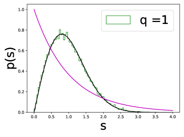
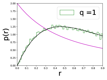
Figure 1: (a) Level spacing $q=1$, $L=24$ unfolded data, which looks approximately like a Wigner-surmise exhibiting level propulsion. In black we plot the Wigner-surmise and in purple we plot the Poisson distribution. (b) Ratio test for spectral statistics at $L=24$. In black we plot the corresponding GOE distribution.

Fig. 1 demonstrates that our model for $q=1$ has level-repulsion and appears to have a level spacing distribution well approximated by the Wigner surmise. While this result shows us that our spectrum strongly resembles the predictions of RMT, the unfolding procedure is usually chosen to find such agreement, therefore it is desirable to perform a test that does not need unfolding. Such a test is given by investigating the distribution of ratios between successive gaps Łydżba et al. (2021c); Oganesyan and Huse (2007); Atas et al. (2013c). We introduce the ratios

$$r_{j}=\frac{\min\{s_{j},s_{j+1}\}}{\max\{s_{j},s_{j+1}\}},$$ (11)

which tells us that $r_{j}\in[0,1]$. We emphasize that the $s_{j}$ we use here don’t need to be unfolded gaps. This test can be done with the model’s physical spectrum. For the GOE in Atas et al. (2013c) it was analytically shown that the distribution of the $r_{j}$ for $3\times 3$ matrices is given by

$$p(r)=\frac{27}{4}\frac{r+r^{2}}{\left(1+r+r^{2}\right)^{\frac{5}{2}}}.$$ (12)

If instead our energy levels were independent randomly distributed variables we would instead get level-attraction,

$$p(r)=\frac{2}{(1+r)^{2}}.$$ (13)

We see in Fig. 1 (b) that our result experiences level-repulsion, agreeing with the distribution in equation 12.

Next we consider the case for $q=2$. The spectrum we are now interested in is equivalent to the spectrum of the Hamiltonian,

$$\hat{H}_{2}=\hat{H}\otimes\mathbb{I}+\mathbb{I}\otimes\hat{H},$$ (14)

which has the spectrum $\Lambda_{k,l}=E_{k}+E_{l}$. This construction introduces an unwanted symmetry in the spectrum of $\hat{H}_{2}$, namely that $\Lambda_{k,l}=\Lambda_{l,k}$, that is, the spectrum is invariant under permutations of the individual energies’ indices. For $q=2$ this might be understood as a spatial reflection symmetry for a larger two component non-interacting system. Addressing this symmetry is simple. We only consider unique pairs of $(k,l)$, namely, we take $l>k$, where we also ignore the portion of the spectrum where $k=l$. Ignoring $k=l$ does not appear to significantly alter the results but allows us to eliminate trivial multiples of the $q=1$ spectrum. In fact, the contribution of the $q=l$ portion of the spectrum is vanishingly small compared to the total size of our spectrum. We further introduce a new index that orders the spectrum $\alpha=1,2\dots$ such that $\Lambda_{\alpha}<\Lambda_{\alpha+1}$. With this new spectrum we can analyze the level spacing and ratio distribution.

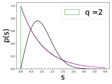
Figure 2: (a) Level spacing $q=2$, $L=20$ unfolded data, which looks approximately like a Poisson distribution. (b) Ratio test for spectral statistics at $L=20$ for $q=2$. In both plots we draw the GOE prediction in black and the independent random variable prediction (Poisson) in purple.

Fig. 2 indicates that the spectrum of $\hat{H}_{2}$ experiences level-attraction. This is contrary to the $q=1$ case which has level-repulsion. Importantly this indicates that the spectrum of $\hat{H}_{2}$ behaves like an integrable model, and has gaps clustered around $s=0$. While this does not guarantee violations of the $q=2$ no-resonance theorem, it does make violations more likely. Likewise, we expect a large amount of pseudo violations such that $s_{j}=\Lambda_{j+1}-\Lambda_{j}\approx 0$, meaning unless very large time scales (potentially non-physically large) are considered these violations would appear as resonances in the spectrum. Considering this fact, results such as Short (2011); Riddell et al. (2022); Srednicki (1999); Mark et al. (2022) should be investigated to understand the effects of resonances. In the appendix B we demonstrate that the Poisson statistics and level-attraction persist for higher values of $q$ and conjecture that level-attraction persists for all values of $q>1$.

One further test we can perform is to test the actual average value of $r$ we observe in the ratio distribution. $\langle r\rangle=2\ln 2-1\approx 0.38629436112$ for Poisson systems and $\langle r\rangle=4-2\sqrt{3}\approx 0.535898384$ for the GOE. Testing this quantity allows us to clearly observe convergence to the predictions of random matrix theory as a function of system size. We see this test in Fig. 3. In the right panel we see the test for $q=2$ which reveals a strong convergence in agreement with the Poisson predictions. The data at $L=22$ gives $\langle r\rangle=0.386294325894$, which confirms seven decimal points of convergence. Therefore, from the perspective of short range correlations in the spectrum we conclude that $\hat{H}_{2}$ obeys Poisson statistics, and importantly, that the $q=2$ case experiences level-attraction.

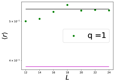
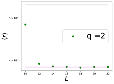
Figure 3: Plotted data for the convergence of $\langle r\rangle$ to RMT predictions. In black we plot the GOE predictions and in purple we plot the corresponding Poisson prediction. Left: We see the $q=1$ data converge to the GOE prediction as a function of system size. Right: We see the $q=2$ data.

In appendix B, we demonstrate that this level-attraction persists for higher values of $q$ and speculate that for all $q>1$ the spectrum must experience level-attraction. In appendix A we repeat our numerical studies but for random matrices, showing that our results from a quantum chaotic Hamiltonian agree with the results of RMT. Importantly our tests here are local tests on the spectrum. It is an open question if the symmetry resolved Hamiltonian $\hat{H}_{2}$ will still obey Poisson statistics for more complex tests such as investigating the spectral form factor Bertini et al. (2021b); Chan et al. (2018b). We leave this question to future work. An important observation from this work is that when studying $q>1$ we never find cases where the spectral statistics aren’t Poisson. In some models such as the tight binding model for free fermions we expect $p(s)$ to be a delta function in the the thermodynamic limit. Crucially, this implies the $q$ no resonance condition is robustly violated for free fermions. We do not observe any such behavior in the spectral statistics for $q>1$ when starting with a chaotic Hamiltonian implying violations should be rare or non-existent.

We emphasize that the presence of level-attraction does not imply violations of the $q>1$ no-resonance condition. It does, however, imply the gaps in the spectrum of $\hat{H}_{2}$ cluster close to zero. If we investigate the probability of finding a gap within the range $0<s<\epsilon$, where $\epsilon$ is small, we have for the GOE,

$$\int_{0}^{\epsilon}\frac{\pi s}{2}e^{-\pi^{2}s^{2}/4}ds=\frac{1-e^{-\frac{-\pi^{2}\epsilon^{2}}{4}}}{\pi}\approx\frac{\pi\epsilon^{2}}{4}-\frac{\pi^{3}\epsilon^{4}}{32}\dots,$$ (15)

so we see the probability is proportional to $\epsilon^{2}$ for small gaps. On the contrary for the Poisson distribution one intuitively yields something much larger,

$$\int_{0}^{\epsilon}e^{-s}ds=\sinh\epsilon-\cosh\epsilon+1\approx\epsilon-\frac{\epsilon^{2}}{2}\dots,$$ (16)

giving us only linear scaling for small gaps. While both probabilities are of course small, the GOE is significantly smaller, giving one a significantly stronger case to assume definition 1 is satisfied in your chaotic model. In the case of Poisson statistics, one might expect to find one or many gaps that are essentially zero due to level-attraction. Infinite time averages are theoretical tools for which we average over times significantly longer than the Heisenberg time $\tau_{H}\sim e^{S}$, where $S$ is the thermodynamic entropy at the appropriate energy $E$ Srednicki (1999). The presence of essentially zero gaps will lead to terms $e^{i(E_{k}-E_{k-1})t}$ which are stationary on time scales proportional to $\tau_{H}$. Despite the presence of such violators, we expect the set of problematic gaps to be small relative to the total Hilbert space dimension. Since it is likely that some violations or cases that are indistinguishable from violations of definition 1 are inevitable, especially for cases using $q>1$, it is instructive to revisit past results keeping in mind a small number of violations will most likely be present. Below we discuss modifying key results in the field of quantum equilibration theory to accommodate the presence of violations of definition 1.

II Equilibration and recurrence

II.1 Physical models

In this section we tackle the problem of equilibration in light of our investigation of the higher order no-resonance conditions and the presence of level-attraction. First, let us review a basic setup. Consider a time independent system with the Hamiltonian $\hat{H}$ where we label the energy eigen basis as $\hat{H}|E_{k}\rangle=E_{k}|E_{k}\rangle$. For simplicity, we take the spectrum of $\hat{H}$ to be discrete and finite. We will initialize our system in some pure state

$$|\psi(t=0)\rangle=\sum_{m}c_{m}|E_{k}\rangle.$$ (17)

To track equilibration, we study properties of the expectation value of an observable $\hat{A}$. This observable is general, but we demand that the largest single value $||A||$ is independent of system size or saturates to a finite value in the thermodynamic limit. In what follows we will assume our spectrum has level-repulsion, so that we may safely assume,

$$E_{m}=E_{l}\implies m=l$$ (18)

.

If our observable equilibrates, its finite time value $\langle\hat{A}(t)\rangle=\langle\psi(t)|\hat{A}|\psi(t)\rangle$ must relax to its infinite time average value i.e.

$$\bar{A}=\lim_{T\to\infty}\frac{1}{T}\int_{0}^{T}\langle\hat{A}(t)\rangle dt=\lim_{T\to\infty}\frac{1}{T}\int_{0}^{T}\sum_{m,n}\bar{c}_{m}c_{n}A_{m,n}e^{i(E_{m}-E_{n})t}dt=\sum_{m}|c_{m}|^{2}A_{m,m}.$$ (19)

$\bar{A}$ is usually written in terms of the diagonal ensemble $\omega=\sum_{m}|c_{m}|^{2}|E_{m}\rangle\langle E_{m}|$ as $\bar{A}=\operatorname{Tr}\left(\omega\hat{A}\right)$. A typical quantity to study in quantum equilibration would be the variance of the expectation value around $\bar{A}$. This was studied and bounded in Short (2011); Reimann and Kastner (2012) assuming that the $q=2$ no-resonance condition was satisfied. The variance is written as

$$\mu_{2}=\lim_{T\to\infty}\frac{1}{T}\int_{0}^{T}\left(\langle\hat{A}(t)\rangle-\bar{A}\right)^{2}dt.$$ (20)

It was famously found in Short (2011) that this variance can be bounded by the purity of the diagonal ensemble

$$\mu_{2}\leq||A||^{2}\operatorname{Tr}\left(\omega^{2}\right).$$ (21)

Note equation 21 holds as a consequence of the $q=2$ no-resonance condition holding. The purity of the diagonal ensemble usually decays exponentially fast with respect to the system size (see for example Fig. 2 in Riddell et al. (2022)). If one assumes higher order $q$ no-resonance conditions, it was recently found that, for higher moments,

$$\mu_{q}=\lim_{T\to\infty}\frac{1}{T}\int_{0}^{T}\left(\langle\hat{A}(t)\rangle-\bar{A}\right)^{q}dt,$$ (22)

a similar bound can be found Riddell et al. (2022),

$$|\mu_{q}|\leq\left(q||A||\sqrt{\operatorname{Tr}\left(\omega^{2}\right)}\right)^{q}.$$ (23)

In light of section I and the presence of level-attraction for higher order $q$, these results should be updated to reflect the high probability of there being a violation of the $q$ no-resonance condition.

Theorem 1.

Suppose we have a model that has violations of the $q$ no-resonance condition. Then the moments $\mu_{q}$ can be bounded as

$$|\mu_{q}|\leq||A||^{q}\left(q^{q}+\frac{\mathcal{N}_{q,L}}{2q}\right)\sqrt{\operatorname{Tr}\left(\omega^{2}\right)}^{q},$$ (24)

where $\mathcal{N}_{q,L}$ is the maximum number of times one $E_{m}$ appears in violations of the $q$ no-resonance condition for a given system size $L$. We call the $E_{m}$’s that appear in more than one violation of the resonance condition exceptional violators.

Proof.

Terms that contribute to $\mu_{q}$ are sums of energies that are equal. Let $\Lambda_{q}$ and $\Lambda_{q}^{\prime}$ be sets of indices corresponding to particular energies,

$$\sum_{m\in\Lambda_{q}}E_{m}=\sum_{m\in\Lambda_{q}^{\prime}}E_{m}.$$ (25)

The no-resonance condition picks out the trivial set of energies that satisfy this equality, which is when $\Lambda_{q}=\Lambda_{q}^{\prime}$. These contributions were bounded in Short (2011); Riddell et al. (2022). We collect the remaining violations in a set $\mathcal{S}$ and write,

$$|\mu_{q}|\leq\left(q||A||\sqrt{\operatorname{Tr}\left(\omega^{2}\right)}\right)^{q}+\left|\sum_{\Lambda_{q}\in\mathcal{S}}\prod_{j=1}^{q}\bar{c}_{m_{j}}c_{n_{j}}A_{m_{j},n_{j}}\right|,$$ (26)

where we have identified $\Lambda_{q}\in\mathcal{S}=\{m_{j},n_{j}\}$. The second term can be bounded as follows.

$$\left|\sum_{\Lambda_{q}\in\mathcal{S}}\prod_{j=1}^{q}\bar{c}_{m_{j}}c_{n_{j}}A_{m_{j},n_{j}}\right|\leq||A||^{q}\sum_{\Lambda_{q}\in\mathcal{S}}\prod_{j=1}^{q}|c_{m_{j}}||c_{n_{j}}|.$$ (27)

Since all $|c_{m_{j}}|$ are positive, we may use the inequality of arithmetic and geometric means, giving

$$\leq\frac{||A||^{q}}{2q}\sum_{\Lambda_{q}\in\mathcal{S}}\sum_{j=1}^{q}\left(|c_{m_{j}}|^{2q}+|c_{n_{j}}|^{2q}\right).$$ (28)

We know that $\operatorname{Tr}\left(\omega^{q}\right)=\sum_{m}|c_{m}|^{2q}$. Assuming an individual $|c_{m_{j}}|^{2q}$ contributes at most $\mathcal{N}_{q,L}$ times, we have that

$$\leq\frac{||A||^{q}\mathcal{N}_{q,L}}{2q}\operatorname{Tr}\left(\omega^{q}\right).$$ (29)

We lastly recall that $\operatorname{Tr}\left(\omega^{q}\right)\leq\operatorname{Tr}\left(\omega^{2}\right)^{q/2}$, which completes the proof. ∎

Accommodating the presence of degenerate gaps for the $q=2$ case has been considered before in Short and Farrelly (2012). Our bound reads,

$$|\mu_{2}|\leq||A||^{2}\left(1+\frac{\mathcal{N}_{2,L}}{4}\right)\operatorname{Tr}\left(\omega^{2}\right).$$ (30)

Instead, one can likewise write Short and Farrelly (2012) as

$$|\mu_{2}|\leq N(\epsilon)||A||^{2}\operatorname{Tr}\left(\omega^{2}\right),$$ (31)

where $N(\epsilon)$ is the maximum number of energy gaps in any interval for $\epsilon>0$, i.e.

$$N(\epsilon)=\max_{E}|\{(k,l)|\enspace E_{k}-E_{l}\in[E,E+\epsilon)\}|.$$ (32)

One can recover the maximum degeneracy of the gaps by considering $\lim_{\epsilon\to 0^{+}}N(\epsilon)$. In the limit of non-degenerate gaps these bounds are identical, and only differ by a constant factor for a small number of degeneracies in the gaps. Our result might in theory give better constant factors than the result in Short and Farrelly (2012), however $N(\epsilon)$ is likely a more intuitive quantity and easier to work with numerically.

We next wish to understand the properties of $\mathcal{N}_{q,L}$, which in practice is challenging to study numerically. The worst scaling it could have is the total number of violations, i.e. $0\leq\mathcal{N}_{q,L}\leq|\mathcal{S}|$. As we have noted earlier, the presence of level-attraction does not imply $|\mathcal{S}|>0$. An easy property to understand however is that if $\mathcal{N}_{q,L}\geq 2$ this implies at the very least that $\mathcal{N}_{q+1,L}\geq 1$. To see this consider $q=2$ for an exceptional violator $E_{m}$ that appears at least twice. We might have $E_{m}$ as an exceptional violator as,

$$E_{m}+E_{n}=E_{p}+E_{l},\enspace E_{m}+E_{k}=E_{r}+E_{h}.$$ (33)

This implies for $q=3$, a violation of the no-resonance condition is

$$E_{p}+E_{l}+E_{k}=E_{r}+E_{h}+E_{n}.$$ (34)

Despite two exceptional violations for $q=2$ implying at least one for $q=3$, this does not imply $\mathcal{N}_{q,L}$ is decreasing in $q$.

To get a handle on the size of $\mathcal{N}_{q,L}$ we can attempt to quantify the expected or average behavior of the quantity. First, let us assume we randomly generated the set $S$. We will assume that the indices which appear are uniformly generated, so each element of $S$ can be understood to be a tuple of $2q$ indices, $(m_{1},\dots m_{2q})$. These indices are not necessarily independent. For example, they cannot be equal to each other under our assumptions. Despite this, in the large $L$ limit this dependence cannot effect results due to the smallness of $q$ and the corresponding exponential nature of the number of possible indices $2^{L}$. We can therefore focus on the first index of each tuple $m_{1}$. Our goal will be to predict the average number of times $m_{1}$ ends up being the same index. It can at most appear $|S|$ times, and thus we wish to compute

$$\langle\mathcal{N}_{q,L}\rangle=\sum_{n=1}^{|S|}np(n),$$ (35)

where $p(n)$ is the probability of the same index appearing $n$ times. The total number of configurations possible for the first index of each tuple in $S$ is $2^{|S|L}$, and therefore we must simply count the number of configurations where $n$ copies of the same $m_{1}$ appear. This is given by

$${|S|\choose n}2^{L\left(|S|-n\right)},$$ (36)

which gives the following formula for our expected value

$$\langle\mathcal{N}_{q,L}\rangle=\sum_{n=0}^{|S|}\frac{n{|S|\choose n}}{2^{Ln}}=\frac{|S|}{2^{L}}(2^{-L}+1)^{|S|-1}.$$ (37)

We now have some special limiting cases to consider. Suppose that $|S|\propto c2^{L}$ for some constant $c$. Then the expected value of $\langle\mathcal{N}_{q,L}\rangle$ is $c\,e^{c}$ as $L$ goes to infinity. However, if $|S|$ has sub exponential growth, for example if it scales as $L$, then the expected value goes to zero for large system size as $\mathcal{O}(L/2^{L})=\mathcal{O}(|S|/2^{L})$. Therefore we expect that for most cases, even with modest violations of the no-resonance condition we expect $\lim_{L\to\infty}N_{q,L}$ to be finite and quite small.

II.2 A Random Matrix Theory Approach

In this section we will show how one could compute $\mu_{q}$ for the GUE and GOE with an unfolded spectrum in the large $N$ limit. We can rewrite equation 22 for finite $T$ as

$$\mu_{q}(T)=\sum_{i_{1},j_{1},...,i_{q},j_{q}}\left(\prod_{k=1}^{q}c_{i_{k}}\overline{c}_{j_{k}}\langle i_{k}|A|j_{k}\rangle\right)\frac{1}{T}\int_{0}^{T}e^{i\sum_{k=1}^{q}(\lambda_{i_{k}}-\lambda_{j_{k}})t}dt,$$ (38)

where the eigenvalues are unfolded and from either a $N\times N$ GUE or GOE distributed matrix. We define its moments as its expectation value.

Define the $n$-level spectral form factor as

$$\mathcal{K}_{2n}^{\overline{\beta}}(t)=\frac{1}{N^{2n}}\left\langle\sum_{i_{1},j_{1},...,i_{n},j_{n}=1}^{N}e^{it\sum_{k=1}^{n}\lambda_{i_{k}}-\lambda_{j_{k}}}\right\rangle_{\overline{\beta}},$$

where the subscript $\overline{\beta}=1$ or 2 denotes the GOE and GUE expectation values, respectively. Then we may express the expectation values of $\mu_{q}$ in terms of its its $q$-level spectral form factor

$$\langle\mu_{q}(T)\rangle_{\overline{\beta}} =\lim_{N\rightarrow\infty}\sum_{i_{1},j_{1},...,i_{q},j_{q}}\left(\prod_{k=1}^{q}c_{i_{k}}\overline{c}_{j_{k}}\langle i_{k}|A|j_{k}\rangle\right)\frac{1}{T}\int_{0}^{T}\left.\langle e^{i\sum_{k=1}^{q}(\lambda_{i_{k}}-\lambda_{j_{k}})t}\right.\rangle_{\overline{\beta}}dt$$ (39)

$$=\left(\frac{1}{T}\int_{0}^{T}\mathcal{K}_{2|B|}^{\overline{\beta}}(t)dt\right)\sum_{i_{1}\not=j_{1},...,i_{q}\not=j_{q}}\left(\prod_{k=1}^{q}c_{i_{k}}c_{j_{k}}\langle i_{k}|A|j_{k}\rangle\right)$$ (40)

$$=\left(\frac{1}{T}\int_{0}^{T}\mathcal{K}_{2|B|}^{\overline{\beta}}(t)dt\right)(\operatorname{Tr}(A\rho-\omega))^{q}.$$ (41)

It is also worth noting that this equation is so general that it applies to any random matrix ensemble. Usually the GUE and GOE are of interest, but progress has been made studying the spectral form factor for other matrix ensembles. For example see Forrester (2021a, b); Cipolloni et al. (2023).

The $q$-level spectral form factor can be computed explicitly, but it is a computationally heavy task. For example see Liu (2018), where it is computed but for ensembles that are not unfolded. In particular, for the GOE and GUE, the 2-level spectral form factor of the unfolded spectrum has a well-known explicit formula in the large $N$ limit Mehta (2004). This leads to the following result.

Theorem 2.

For any fixed $T$ greater than zero, the GOE and GUE the expectation value of $\mu_{2}(T)$ goes to zero as $1/N^{2}$ in the large $N$ limit. Furthermore, if $T$ goes to infinity at the same rate as $N$ (i.e. $N=T$) then $\mu_{2}(T)$ goes to zero as $1/T$.

Proof.

From Mehta (2004); Cipolloni et al. (2023), we know that for large $N$ the spectral form factors can be approximated by

$$\mathcal{K}_{2}^{1}(t)\approx\left\{\begin{array}[]{lr}\frac{4t}{\pi N^{2}}+\frac{2t}{\pi N^{2}}\ln(1+\frac{4t}{\pi N})&\text{if }0\leq t\leq\frac{\pi N}{2}\\ \frac{2}{N}+\frac{2t}{\pi N^{2}}\ln\left(\frac{\frac{4t}{\pi N}+1}{\frac{4t}{\pi N}-1}\right)&\text{if }t\geq\frac{\pi N}{2}\end{array}\right.$$ (42)

and

$$\mathcal{K}_{2}^{2}(t)\approx\left\{\begin{array}[]{lr}\frac{2t}{\pi N^{2}}&\text{if }0\leq t\leq\frac{\pi N}{2}\\ \frac{1}{N}&\text{if }t\geq\frac{\pi N}{2}\end{array}\right..$$ (43)

Clearly, the first part of every piecewise function will dominate for large $N$, thus completing the first claim.

Next, set $T=N$. Taking the above quantities time averages we get

$$\frac{1}{T}\int_{0}^{T}\mathcal{K}_{2}^{1}(t)dt\approx\frac{1}{T}\left(\frac{3}{2\,\pi}-{\frac{\pi}{16}\ln\left(1+{\frac{4}{\pi}}\right)}+{\frac{1}{\pi}\ln\left(1+{\frac{4}{\pi}}\right)}+{\frac{3\,\pi}{32}}+{\frac{1}{4}}\right)$$ (44)

and

$$\frac{1}{T}\int_{0}^{T}\mathcal{K}_{2}^{2}(t)dt\approx\frac{1}{\pi\,T}.$$ (45)

This proves the second claim. ∎

As we demonstrate in appendix A, the spectrum of the random matrix Hamiltonian likewise experiences level-attraction for $q\geq 2$. However, despite the presence of level-attraction, the above RMT result indicates that we still should expect $\mu_{q}\to 0$ indicating equilibration on average of our observable.

III Conclusion

In this work we have explored spectral statistics of chaotic Hamiltonians, namely the statistics surrounding sums of energies. We found that despite being chaotic, sums of energies displayed Poisson statistics instead of Wigner-Dyson statistics. This was demonstrated numerically for both a chaotic spin Hamiltonian and the GOE. The presence of level-attraction leads one to believe that accounting for potential degeneracies or “resonances” in infinite time averages of some dynamical quantities is necessary. We applied this observation to the theory of equilibration where we generalized known bounds to accommodate for degeneracies. Assuming the number of degeneracies is not exponentially large in system size, we demonstrated that the the bounds can be easily generalized to accomondate the presence of resonances. We further used techniques from RMT to prove that, for the GOE, moments of equilibration go to zero in the thermodynamic limit.

IV Acknowledgements

J.R. would like to thank Bruno Bertini, Marcos Rigol and Alvaro Alhambra for fruitful conversations. J.R. would like to extend special thanks in particular to Bruno who gave valuable feedback at various stages of the project. J.R. acknowledges the support of Royal Society through the University Research Fellowship No. 201101. N.J.P. acknowledges support from the Natural Sciences and Engineering Research Council of Canada (NSERC).

Appendix A RMT predictions for $q=2,3$

In this section we demonstrate that random matrix models have level-attraction for $q=2,3$. We accomplish this by simply looking at the ratio test outlined in the main text. First let us define a random matrix Hamiltonian,

$$\hat{H}=A+A^{T},$$ (46)

where $A$ is a matrix filled with random numbers generated from a normal distribution with zero mean and unit variance. We label the side length of $A$ as $N$. Similar to the physical Hamiltonian, we can study the $q=2$ case by first constructing the Hamiltonian,

$$\hat{H}_{2}=\hat{H}\otimes\mathbb{I}+\mathbb{I}\otimes\hat{H},$$ (47)

with the spectrum $\Lambda_{k,l}$. Again this spectrum is symmetric under permutations of the indices, so we resolve this symmetry and only treat eigenvalues with unique $(k,l)$ such that $l>k$. We investigate the spectral properties of this Hamiltonian after resolving our symmetry in figure 4 in the left panel. Here we clearly see agreement with a Poisson distribution. The random matrix model experiences level-attraction.

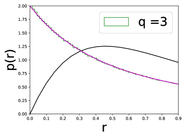
Figure 4: (a) Ratio test for the $q=2$ symmetry resolved random matrix Hamiltonian. Side length is $N=1200$. (b) Ratio test for the $q=3$ symmetry resolved random matrix Hamiltonian. Side length is $N=200$.

The construction of a new Hamiltonian for $q=3$ is similar. We have

$$\hat{H}_{3}=\hat{H}\otimes\mathbb{I}\otimes\mathbb{I}+\mathbb{I}\otimes\hat{H}\otimes\mathbb{I}+\mathbb{I}\otimes\mathbb{I}\otimes\hat{H}.$$ (48)

This gives us a new spectrum of $\Lambda_{k,l,q}=E_{k}+E_{l}+E_{q}$, where this new spectrum is also invariant under permutations of its indices. We resolve this symmetry by considering terms such that $q>l>k$. The result of the ratio test on this new spectrum is given in the right panel of Fig. 4, indicating again level-attraction and agreement with Poisson statistics. This is similarly found for higher values of $q$, which leads us to conjecture that this will be true for all $q\geq 2$.

Appendix B Physical Hamiltonian q = 3,4 spectral statistics

In this section we provide numerical evidence for level-attraction for $q=3,4$ in the physical Hamiltonian. We repeat the $q=3$ case as was covered in the RMT appendix, and also investigate the $q=4$ statistics. Both cases will be covered with the ratio test, and we will use the same physical model as the main text, where we resolve all relevant symmetries. For the $q=4$ case, we must work with the Hamiltonian,

$$\hat{H}_{4}=\hat{H}\otimes\mathbb{I}\otimes\mathbb{I}\otimes\mathbb{I}+\mathbb{I}\otimes\hat{H}\otimes\mathbb{I}\otimes\mathbb{I}+\mathbb{I}\otimes\mathbb{I}\otimes\hat{H}\otimes\mathbb{I}+\mathbb{I}\otimes\mathbb{I}\otimes\mathbb{I}\otimes\hat{H}.$$ (49)

This gives us a new spectrum, again which is invariant under index permutations. We can resolve this symmetry with an identical strategy to the $q=2,3$ cases, and study the corresponding symmetry-resolved spectrum. The results of this for $q=3,4$ in the physical Hamiltonian are given in Fig. 5. These results again indicate that the spectrum has level-attraction and obeys Poisson statistics. The left panel in Fig. 5 also serves as evidence that the statistics of the Hamiltonian agrees with RMT as seen in the right panel of Fig. 4.

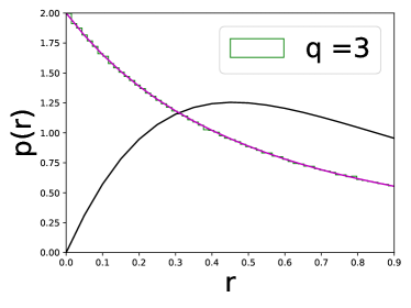
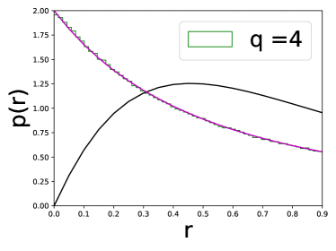
Figure 5: (a) Ratio test for the $q=3$ symmetry resolved physical Hamiltonian. The physical Hamiltonian $\hat{H}$ is generated with $L=16$. (b) Ratio test for the $q=4$ symmetry resolved physical Hamiltonian. The Hamiltonian $\hat{H}$ here has $L=14$.

References

- Berry (1987) M. V. Berry, Proc. R. Soc. A 413, 183 (1987).
- D’Alessio et al. (2016) L. D’Alessio, Y. Kafri, A. Polkovnikov, and M. Rigol, Advances in Physics 65, 239 (2016).
- Porter (1965) C. E. Porter, Statistical theories of spectra: fluctuations, Tech. Rep. (1965).
- Brody et al. (1981) T. A. Brody, J. Flores, J. B. French, P. Mello, A. Pandey, and S. S. Wong, Reviews of Modern Physics 53, 385 (1981).
- Guhr et al. (1998) T. Guhr, A. Müller-Groeling, and H. A. Weidenmüller, Physics Reports 299, 189 (1998).
- Berry and Tabor (1976) M. V. Berry and M. Tabor, Proc. R. Soc. A 349, 101 (1976).
- Berry and Tabor (1977) M. V. Berry and M. Tabor, Proc. R. Soc. A 356, 375 (1977).
- Jalabert et al. (1990) R. A. Jalabert, H. U. Baranger, and A. D. Stone, Phys. Rev. Lett. 65, 2442 (1990).
- Marcus et al. (1992) C. M. Marcus, A. J. Rimberg, R. M. Westervelt, P. F. Hopkins, and A. C. Gossard, Phys. Rev. Lett. 69, 506 (1992).
- Milner et al. (2001) V. Milner, J. L. Hanssen, W. C. Campbell, and M. G. Raizen, Phys. Rev. Lett. 86, 1514 (2001).
- Friedman et al. (2001) N. Friedman, A. Kaplan, D. Carasso, and N. Davidson, Phys. Rev. Lett. 86, 1518 (2001).
- Stockmann and Stein (1990) H. J. Stockmann and J. Stein, Phys. Rev. Lett. 64, 2215 (1990).
- Sridhar (1991) S. Sridhar, Phys. Rev. Lett. 67, 785 (1991).
- Moore et al. (1994) F. L. Moore, J. C. Robinson, C. Bharucha, P. E. Williams, and M. G. Raizen, Phys. Rev. Lett. 73, 2974 (1994).
- Steck et al. (2001) D. A. Steck, W. H. Oskay, and M. G. Raizen, Science 293, 274 (2001).
- Hensinger et al. (2001) W. K. Hensinger, H. Häffner, A. Browaeys, N. R. Heckenberg, K. Helmerson, C. McKenzie, G. J. Milburn, W. D. Phillips, S. L. Rolston, H. Rubinsztein-Dunlop, and B. Upcroft, Nature 412, 52 (2001).
- Chaudhury et al. (2009) S. Chaudhury, A. Smith, B. E. Anderson, S. Ghose, and P. S. Jessen, Nature 461, 768 (2009).
- Weinstein et al. (2002) Y. S. Weinstein, S. Lloyd, J. Emerson, and D. G. Cory, Phys. Rev. Lett. 89, 157902 (2002).
- Zhang et al. (2022) Y. Zhang, L. Vidmar, and M. Rigol, Phys. Rev. E 106, 014132 (2022).
- Łydżba et al. (2021a) P. Łydżba, Y. Zhang, M. Rigol, and L. Vidmar, Phys. Rev. B 104, 214203 (2021a).
- Łydżba et al. (2021b) P. Łydżba, M. Rigol, and L. Vidmar, Phys. Rev. B 103, 104206 (2021b).
- Santos and Rigol (2010a) L. F. Santos and M. Rigol, Phys. Rev. E 81, 036206 (2010a).
- Santos and Rigol (2010b) L. F. Santos and M. Rigol, Phys. Rev. E 82, 031130 (2010b).
- Rigol (2010) M. Rigol, ArXiv e-prints (2010), arXiv:1008.1930 [cond-mat.stat-mech] .
- Kollath et al. (2010) C. Kollath, G. Roux, G. Biroli, and A. M. Läuchli, Journal of Statistical Mechanics: Theory and Experiment 2010, P08011 (2010).
- Santos et al. (2012) L. F. Santos, A. Polkovnikov, and M. Rigol, Physical Review E 86 (2012), 10.1103/physreve.86.010102.
- Richter et al. (2020) J. Richter, A. Dymarsky, R. Steinigeweg, and J. Gemmer, Physical Review E 102 (2020), 10.1103/physreve.102.042127.
- Atas et al. (2013a) Y. Y. Atas, E. Bogomolny, O. Giraud, and G. Roux, Phys. Rev. Lett. 110, 084101 (2013a).
- Atas et al. (2013b) Y. Y. Atas, E. Bogomolny, O. Giraud, P. Vivo, and E. Vivo, Journal of Physics A: Mathematical and Theoretical 46, 355204 (2013b).
- untajs et al. (2020) J. untajs, J. Bona, T. c. v. Prosen, and L. Vidmar, Phys. Rev. E 102, 062144 (2020).
- Chan et al. (2018a) A. Chan, A. De Luca, and J. Chalker, Phys. Rev. X 8, 041019 (2018a).
- D’Alessio and Rigol (2014) L. D’Alessio and M. Rigol, Phys. Rev. X 4, 041048 (2014).
- Bertini et al. (2021a) B. Bertini, P. Kos, and T. Prosen, Communications in Mathematical Physics 387, 597 (2021a).
- Bertini et al. (2018) B. Bertini, P. Kos, and T. c. v. Prosen, Phys. Rev. Lett. 121, 264101 (2018).
- Dyson (1962a) F. J. Dyson, Journal of Mathematical Physics 3, 140 (1962a).
- Dyson (1962b) F. J. Dyson, Journal of Mathematical Physics 3, 157 (1962b).
- Dyson (1962c) F. J. Dyson, Journal of Mathematical Physics 3, 166 (1962c).
- Dyson and Mehta (1963) F. J. Dyson and M. L. Mehta, Journal of Mathematical Physics 4, 701 (1963).
- Mehta and Dyson (1963) M. Mehta and F. Dyson, Journal of Mathematical Physics (New York)(US) 4 (1963).
- Dyson (1962d) F. J. Dyson, Journal of Mathematical Physics 3, 1199 (1962d).
- Bohigas et al. (1984) O. Bohigas, M.-J. Giannoni, and C. Schmit, Physical review letters 52, 1 (1984).
- Bohrdt et al. (2017) A. Bohrdt, C. B. Mendl, M. Endres, and M. Knap, New. J. Phys. 19, 063001 (2017).
- Andreev et al. (1996) A. Andreev, O. Agam, B. Simons, and B. Altshuler, Physical review letters 76, 3947 (1996).
- Müller et al. (2004) S. Müller, S. Heusler, P. Braun, F. Haake, and A. Altland, Physical review letters 93, 014103 (2004).
- Mehta (2004) M. L. Mehta, Random matrices (Elsevier, 2004).
- Bruus and Angl‘es d’Auriac (1997) H. Bruus and J.-C. Angl‘es d’Auriac, Phys. Rev. B 55, 9142 (1997).
- Mehta (1960) M. L. Mehta, Nuclear Physics 18, 395 (1960).
- Jimbo et al. (1980) M. Jimbo, T. Miwa, Y. Mori, and M. Sato, Physica D: Nonlinear Phenomena 1, 80 (1980).
- Forrester and Witte (2000) P. Forrester and N. Witte, Letters in Mathematical Physics 53, 195 (2000).
- Livan et al. (2018) G. Livan, M. Novaes, and P. Vivo, Monograph Award 63 (2018).
- Alhambra et al. (2020) Á. M. Alhambra, J. Riddell, and L. P. García-Pintos, Phys. Rev. Lett. 124, 110605 (2020).
- Riddell and Sørensen (2020) J. Riddell and E. S. Sørensen, Phys. Rev. B 101, 024202 (2020).
- Gogolin and Eisert (2016) C. Gogolin and J. Eisert, Rep. Prog. Phys. 79, 056001 (2016).
- Masanes et al. (2013) L. Masanes, A. J. Roncaglia, and A. Acín, Phys. Rev. E 87, 032137 (2013).
- Wilming et al. (2018) H. Wilming, T. R. de Oliveira, A. J. Short, and J. Eisert, in Thermodynamics in the Quantum Regime (Springer, 2018) pp. 435–455.
- Heveling et al. (2020) R. Heveling, L. Knipschild, and J. Gemmer, Journal of Physics A: Mathematical and Theoretical 53, 375303 (2020).
- Campos Venuti and Zanardi (2010) L. Campos Venuti and P. Zanardi, Phys. Rev. A 81 (2010), 10.1103/physreva.81.022113.
- Knipschild and Gemmer (2020) L. Knipschild and J. Gemmer, Physical Review E 101 (2020), 10.1103/physreve.101.062205.
- Carvalho et al. (2023) G. D. Carvalho, L. F. dos Prazeres, P. S. Correia, and T. R. de Oliveira, (2023), arXiv:2305.11985 [quant-ph] .
- Riddell et al. (2021) J. Riddell, W. Kirkby, D. H. J. O’Dell, and E. S. Sørensen, “Scaling at the otoc wavefront: Integrable versus chaotic models,” (2021), arXiv:2111.01336 [cond-mat.stat-mech] .
- Riddell and Sørensen (2019) J. Riddell and E. S. Sørensen, Physical Review B 99, 054205 (2019).
- Yoshida and Yao (2019) B. Yoshida and N. Y. Yao, Phys. Rev. X 9, 011006 (2019).
- Fortes et al. (2019) E. M. Fortes, I. García-Mata, R. A. Jalabert, and D. A. Wisniacki, Phys. Rev. E 100, 042201 (2019).
- Shukla et al. (2022) R. K. Shukla, A. Lakshminarayan, and S. K. Mishra, Phys. Rev. B 105, 224307 (2022).
- Fortes et al. (2020) E. M. Fortes, I. García-Mata, R. A. Jalabert, and D. A. Wisniacki, Europhysics Letters 130, 60001 (2020).
- Mark et al. (2022) D. K. Mark, J. Choi, A. L. Shaw, M. Endres, and S. Choi, “Benchmarking quantum simulators using quantum chaos,” (2022).
- Srednicki (1999) M. Srednicki, Journal of Physics A: Mathematical and General 32, 1163 (1999).
- Riddell et al. (2022) J. Riddell, N. Pagliaroli, and Á. M. Alhambra, arXiv preprint arXiv:2206.07541 (2022).
- Khalkhali and Pagliaroli (2022) M. Khalkhali and N. Pagliaroli, Journal of Mathematical Physics 63, 053504 (2022).
- LeBlond et al. (2019) T. LeBlond, K. Mallayya, L. Vidmar, and M. Rigol, Phys. Rev. E 100, 062134 (2019).
- Łydżba et al. (2021c) P. Łydżba, M. Rigol, and L. Vidmar, Phys. Rev. B 103, 104206 (2021c).
- Oganesyan and Huse (2007) V. Oganesyan and D. A. Huse, Physical review b 75, 155111 (2007).
- Atas et al. (2013c) Y. Atas, E. Bogomolny, O. Giraud, and G. Roux, Physical review letters 110, 084101 (2013c).
- Short (2011) A. J. Short, New. J. Phys. 13, 053009 (2011).
- Bertini et al. (2021b) B. Bertini, P. Kos, and T. Prosen, Communications in Mathematical Physics 387, 597 (2021b).
- Chan et al. (2018b) A. Chan, A. De Luca, and J. T. Chalker, Phys. Rev. X 8, 041019 (2018b).
- Reimann and Kastner (2012) P. Reimann and M. Kastner, New Journal of Physics 14, 043020 (2012).
- Short and Farrelly (2012) A. J. Short and T. C. Farrelly, New. J. Phys. 14, 013063 (2012).
- Forrester (2021a) P. J. Forrester, Journal of Statistical Physics 183, 33 (2021a).
- Forrester (2021b) P. J. Forrester, Communications in Mathematical Physics 387, 215 (2021b).
- Cipolloni et al. (2023) G. Cipolloni, L. Erdős, and D. Schröder, Communications in Mathematical Physics , 1 (2023).
- Liu (2018) J. Liu, Physical Review D 98, 086026 (2018).