Accreting luminous low-mass planets escape from migration traps at pressure bumps

Abstract

We investigate the migration of Mars- to super-Earth-sized planets in the vicinity of a pressure bump in a 3D radiative protoplanetary disc while accounting for the effect of accretion heat release. Pressure bumps have often been assumed to act as efficient migration traps, but we show that the situation changes when the thermal forces are taken into account. Our simulations reveal that for planetary masses $\lesssim$$2\,M_{\earth}$, once their luminosity exceeds the critical value predicted by linear theory, thermal driving causes their orbits to become eccentric, quenching the positive corotation torque responsible for the migration trap. As a result, planets continue migrating inwards past the pressure bump. Additionally, we find that planets that remain circular and evolve in the super-Keplerian region of the bump exhibit a reversed asymmetry of their thermal lobes, with the heating torque having an opposite (negative) sign compared to the standard circular case, thus leading to inward migration as well. We also demonstrate that the super-critical luminosities of planets in question can be reached through the accretion of pebbles accumulating in the bump. Our findings have implications for planet formation scenarios that rely on the existence of migration traps at pressure bumps, as the bumps may repeatedly spawn inward-migrating low-mass embryos rather than harbouring newborn planets until they become massive.

1 Introduction

The recent advancements of interferometric observations with high angular resolution have enabled to detect ring-like concentrations of small solid particles (dust or pebbles) in numerous protoplanetary discs (e.g. Andrews et al., 2018; Dipierro et al., 2018; Cieza et al., 2019). Such ring-shaped accumulations could have formed at the locations of pressure bumps where the disc rotation becomes locally super-Keplerian and the inward drift of small solids due to the aerodynamic drag is blocked (Nakagawa et al., 1986; Dullemond et al., 2018; Teague et al., 2018).

Since pressure bumps overlap with transitions in the gas density, they can act as barriers for planetary migration due to a local boost of the positive corotation torque, which balances the negative Lindblad torque (e.g. Masset et al., 2006; Ataiee & Kley, 2021; Chrenko et al., 2022). Therefore, a pressure bump could hypothetically represent a sweat spot for planet formation: Any planet growing at the bump would be protected from planetary migration and it would remain submerged in a relatively dense and self-replenishing reservoir of solids from which it could continue accreting. Such an interplay has become a key component of many novel planet formation scenarios (Morbidelli, 2020; Guilera et al., 2020; Chambers, 2021; Andama et al., 2022; Lau et al., 2022; Jiang & Ormel, 2023).

However, the existence of the migration trap at the pressure bump has so far been justified by taking only the Lindblad and corotation disc-driven torques (Goldreich & Tremaine, 1979; Ward, 1991; Masset, 2001; Tanaka et al., 2002) into account and thus, from the viewpoint of planet-disc interactions, the picture is not entirely complete. In non-isothermal discs with any form of thermal diffusion, planets are subject to additional thermal torques (Masset, 2017). When the planet is non-luminous, the gas traveling past the planet gains energy by compressional heating but this energy is spread by thermal diffusion (Lega et al., 2014) and a perturbation arises which is cooler and denser compared to a fully adiabatic case. When the planet is accreting and luminous, a threshold luminosity exists for which the disc perturbation is similar to the fully adiabatic case (Masset, 2017). Planets with super-critical luminosities switch to the regime of the heating torque (Benítez-Llambay et al., 2015; Hankla et al., 2020; Chametla & Masset, 2021).

The heating torque arises because the accretion heat renders the gas flowing past the planet underdense. The underdense gas is redistributed by the thermal (or radiative) diffusion and disc shear and two lobes are formed, the inner lobe leading and the outer lobe trailing the orbital motion of the planet (Benítez-Llambay et al., 2015; Masset, 2017). For a typical sub-Keplerian disc and a circular planetary orbit, the outer trailing lobe is more pronounced because the corotation radius between the planet and the disc material is shifted inwards. We recall, however, that Chrenko & Lambrechts (2019) showed that the advection of hot gas near super-Earth-sized planets is not governed purely by the shear motion but rather by a complex 3D circumplanetary flow interacting with the horseshoe region of the planet (see also Chametla & Masset, 2021).

Additionally, the perturbing force acting upon the luminous planet can also excite its orbital eccentricity (Chrenko et al., 2017; Eklund & Masset, 2017; Fromenteau & Masset, 2019; Velasco Romero et al., 2022; Cornejo et al., 2023). When that happens, the two thermal lobes are replaced with a single lobe whose trajectory can be well approximated with an epicycle and the planet is said to enter the headwind-dominated regime of thermal torques (Eklund & Masset, 2017). While the heating torque is typically positive and supports outward migration in the circular shear-dominated regime (Benítez-Llambay et al., 2015; Masset, 2017), its contribution to the overall torque balance in the eccentric headwind-dominated regime is less clear.

In our study, we investigate the migration of pebble-accreting planets in the vicinity of the pressure bump while taking the thermal torques into account, with the aim to answer the following questions. Will the thermal torques assist or counteract the migration trap? Will the orbital eccentricity grow and if so, how will the torque balance change? By carrying out an extensive set of numerical simulations, we show that planets with super-critical luminosities are likely to experience the eccentricity excitation and enter the headwind-dominated regime. The subsequent orbital migration of such planets is dominated by the Lindblad torque because the corotation torque is quenched for eccentric orbits (Bitsch & Kley, 2010; Fendyke & Nelson, 2014) and we demonstrate that the influence of the thermal torque on the evolution of the semi-major axis weakens as well (see also Pierens, 2023). Finally, for parameters that allow the planet to remain in the circular shear-dominated regime, we show that the thermal torques in the super-Keplerian region of the pressure bump have an opposite effect compared to Benítez-Llambay et al. (2015).

2 3D radiative hydrodynamic model

We model a patch of a 3D gas disc on an Eulerian grid with uniform spacing and $N_{r}\times N_{\theta}\times N_{\phi}$ cells, where the subscripts stand for the radial, azimuthal, and colatitudinal spherical coordinates, respectively. The azimuthal extent of the grid for our simulations with planets covers a quadrant, not the full azimuth (see Section 2.1). We use the Fargo3D code (Benítez-Llambay & Masset, 2016) and treat the gas disc as a viscous fluid evolving in a non-inertial frame centered on the star $M_{\star}$ and co-rotating with an embedded planet $M_{\mathrm{p}}$, whose orbital evolution we study. The gravitational potential of the planet is smoothed with the cubic spline function of Klahr & Kley (2006) at cell-planet distances $d<r_{\mathrm{sm}}$, where $r_{\mathrm{sm}}$ is the smoothing length (Table 1), as

$$\Phi_{\mathrm{p}}=-\frac{GM_{\mathrm{p}}}{d}\left[\left(\frac{d}{r_{\mathrm{sm}}}\right)^{4}-2\left(\frac{d}{r_{\mathrm{sm}}}\right)^{3}+2\frac{d}{r_{\mathrm{sm}}}\right]\,,$$ (1)

where $G$ is the gravitational constant.

Aside from the continuity and momentum equations that are included in the public version of Fargo3D (Benítez-Llambay & Masset, 2016), we consider the evolution of the internal energy density of the gas $\epsilon$ and the energy density of diffuse thermal radiation $E_{\mathrm{R}}$ following the two-temperature approximation (Commerçon et al., 2011; Bitsch et al., 2013):

$$\frac{\partial E_{\mathrm{R}}}{\partial t}+\nabla\cdot\vec{F}=\rho\kappa_{\mathrm{P}}\left[4\sigma T^{4}-cE_{\mathrm{R}}\right]\,,$$ (2)

$$\frac{\partial\epsilon}{\partial t}+\nabla\cdot\left(\epsilon\vec{v}\right)=-\rho\kappa_{\mathrm{P}}\left[4\sigma T^{4}-cE_{\mathrm{R}}\right]-P\nabla\cdot\vec{v}+Q_{\mathrm{visc}}+Q_{\mathrm{art}}+Q_{\mathrm{acc}}\,,$$ (3)

where $t$ is the time, $\vec{F}$ is the radiation flux vector, $\rho$ is the gas density, $\kappa_{\mathrm{P}}$ is the Planck opacity, $\sigma$ is the Stefan-Boltzmann constant, $T$ is the gas temperature, $c$ is the speed of light, $\vec{v}=(v_{r},v_{\theta},v_{\phi})$ is the velocity vector of the gas flow, $P$ is the gas pressure ($P=(\gamma-1)\epsilon$ for the ideal gas with the adiabatic index $\gamma$), $Q_{\mathrm{visc}}$ is the viscous heating term (Mihalas & Weibel Mihalas, 1984), $Q_{\mathrm{art}}$ is the heating due to the shock-spreading viscosity of finite-difference codes (Stone & Norman, 1992), and $Q_{\mathrm{acc}}$ is the heat source related to the luminosity of the embedded planet. For the implementation of the energy equations, the flux-limited approximation, and the remaining closure relations, the reader is referred to Chrenko & Lambrechts (2019) and references therein. Let us only point out that the Planck and Rosseland opacities (the latter of which governs the radiation diffusion) assumed here are uniform and equal, $\kappa_{\mathrm{P}}=\kappa_{\mathrm{R}}=\kappa$. Equations (2) and (3) are solved implicitly using the successive over-relaxation method with the relative precision of $10^{-8}$.

To model the heat release due to planetary accretion, we consider a simple luminosity relation (Benítez-Llambay et al., 2015)

$$L=\frac{GM_{\mathrm{p}}\dot{M_{\mathrm{p}}}}{R_{\mathrm{p}}}=\frac{GM_{\mathrm{p}}^{2}}{R_{\mathrm{p}}\tau}\,,$$ (4)

where $\dot{M_{\mathrm{p}}}$ is the mass accretion rate of the planet, $R_{\mathrm{p}}$ is its physical radius, and $\tau=M_{\mathrm{p}}/\dot{M_{\mathrm{p}}}$ is its mass doubling time. Let us point out that $\tau$ is used only to regulate $L$ but $M_{\mathrm{p}}$ itself is kept fixed throughout our simulations. The heat source is non-zero in eight cells surrounding the planet (Benítez-Llambay et al., 2015) and zero elsewhere. To account for the shift of the planet with respect to these cells, we define the grid coordinates of the planet $(r_{\mathrm{p}},\theta_{\mathrm{p}},\phi_{\mathrm{p}})$, coordinates of an $n$-th cell centre $(r_{n},\theta_{n},\phi_{n})$, dimensions of the respective cell $(\Delta r,\Delta\theta,\Delta\phi)$, its volume $V_{n}$, and apply (e.g. Velasco Romero et al., 2022)

$$Q_{\mathrm{acc},n}=\frac{L}{V_{n}}\left(1-\frac{|r_{\mathrm{p}}-r_{n}|}{\Delta r}\right)\left(1-\frac{|\theta_{\mathrm{p}}-\theta_{n}|}{\Delta\theta}\right)\left(1-\frac{|\phi_{\mathrm{p}}-\phi_{n}|}{\Delta\phi}\right)\,,$$ (5)

inside cells that satisfy $|r_{\mathrm{p}}-r_{n}|<\Delta r$, $|\theta_{\mathrm{p}}-\theta_{n}|<\Delta\theta$, and $|\phi_{\mathrm{p}}-\phi_{n}|<\Delta\phi$.

Most of our simulations are performed on a (i) disc quadrant and with (ii) migrating planets. Due to (i), it is not possible to consider the indirect potential term related to the acceleration of the star generated by the disc. Point (ii) motivates us to subtract the azimuthally-averaged gas density from $\rho$ before the disc-planet interaction is evaluated (Baruteau & Masset, 2008). Such a procedure improves the displacement of the Lindblad resonances in a non-self-gravitating disc. The planetary orbit is propagated using the standard fourth-order Runge-Kutta integrator of Fargo3D.

Table 1: Fixed parameters for simulations with embedded planets (simulations of disc relaxation differ in the grid span and resolution; Section 2.1). Below, $r_{\mathrm{p}}$ marks the initial radial planet position and $R_{\mathrm{H}}$ is the planet’s Hill radius.

Parameter	Notation	Value
Grid resolution	$N_{r}\times N_{\theta}\times N_{\phi}$	$1536\times 4096\times 128$
Radial grid span	$(r_{\mathrm{min}},r_{\mathrm{max}})$	$(0.7,1.3)\,r_{\mathrm{p}}$
Azimuthal grid span	$(\theta_{\mathrm{min}},\theta_{\mathrm{max}})$	$(-\pi/4,\pi/4)$
Vertical grid span	$(\phi_{\mathrm{min}},\phi_{\mathrm{max}})$	$(7\pi/15,\pi/2)$
Stellar mass	$M_{\star}$	$1\,M_{\sun}$
Surface density (at 1 au)	$\Sigma_{0}$	$456\,\mathrm{g}\,\mathrm{cm}^{-2}$
Adiabatic index	$\gamma$	$1.43$
Mean molecular weight	$\mu$	$2.3$
Kinematic viscosity	$\nu$	$10^{15}\,\mathrm{cm}^{2}\,\mathrm{s}^{-1}$
Opacity	$\kappa$	$1\,\mathrm{cm}^{2}\,\mathrm{g}^{-1}$
Bump amplitude	$A_{\mathrm{b}}$	$1.45$
Bump centre	$r_{\mathrm{b}}$	$5.2\,\mathrm{au}$
Bump width	$w_{\mathrm{b}}$	$0.32\,\mathrm{au}$
Smoothing length	$r_{\mathrm{sm}}$	$0.15\,R_{\mathrm{H}}$

2.1 Initial conditions with a pressure bump

Before conducting simulations with embedded planets, it is imperative to find an equilibrium state of the unperturbed disc determined by the balance between viscous heating and radiative cooling. We start with a disc that has a radial extension of $(r_{\mathrm{min}},r_{\mathrm{max}})=(2.6,7.8)\,\mathrm{au}$ and a grid resolution of $N_{r}\times N_{\theta}\times N_{\phi}=768\times 1\times 64$. The disc is azimuthally symmetric (as represented by $N_{\theta}=1$) as well as vertically symmetric around the midplane (only one hemisphere of the disc is modelled). Remaining parameters are the same as in Table 1.

The initial temperature profile is that of an optically thin disc (e.g. Ueda et al., 2017) and the initial surface density profile follows

$$\Sigma(r)=\Sigma_{0}\left(\frac{r}{1\,\mathrm{au}}\right)^{-0.5}\,.$$ (6)

We introduce the pressure bump as a Gaussian perturbation of the surface density (Pinilla et al., 2012; Dullemond et al., 2018)

$$\Sigma^{\prime}(r)=\Sigma(r)\left[1+(A_{\mathrm{b}}-1)\exp{\left(-\frac{(r-r_{\mathrm{b}})^{2}}{2w_{\mathrm{b}}^{2}}\right)}\right]\,,$$ (7)

where $A_{\mathrm{b}}$ is the bump amplitude, $r_{\mathrm{b}}$ is the radial centre of the perturbation, and $w_{\mathrm{b}}$ parametrizes the width of the Gaussian. To minimize the viscous spreading over the course of our simulations, we ‘mirror’ the Gaussian perturbation as a minimum in the viscosity profile (e.g. Ataiee et al., 2014)

$$\nu^{\prime}(r)=\nu\left[1+(A_{\mathrm{b}}-1)\exp{\left(-\frac{(r-r_{\mathrm{b}})^{2}}{2w_{\mathrm{b}}^{2}}\right)}\right]^{-1}\,.$$ (8)

Let us point out that in the absence of the pressure bump, the disc would be similar to that of Eklund & Masset (2017).

The first part of our relaxation procedure is hydrostatic and iterative. For a given temperature field, we solve the equations of hydrostatic equilibrium (Flock et al., 2016; Chrenko & Nesvorný, 2020) to find a new density distribution $\rho(r,\phi)$. Then we fix the new density distribution and perform one time step equal to the characteristic radiation diffusion time-scale in the energy equations. With the updated temperature field, the iteration process is repeated until the relative change in $T$ and $\rho$ per iteration becomes as small as $10^{-5}$.

In the second step of our relaxation procedure, we continue to evolve the disc using the full set of time-dependent fluid equations over 2,000 orbital time-scales at $r_{\mathrm{b}}$. To insert a planet at an arbitrary position $r_{\mathrm{p}}$ in the disc, we remap the relaxed disc to a numerical grid with the radial extension of $(r_{\mathrm{min}},r_{\mathrm{max}})=(0.7,1.3)\,r_{\mathrm{p}}$ and an azimuthal extension of a quadrant. The resolution of the remapped grid is given in Table 1. We also transform the azimuthal gas velocity $v_{\theta}$ to a frame corotating with the planet. If the planet starts in an eccentric orbit, the frame velocity is corrected for the eccentricity (planets start in their apocentre).

2.2 Boundary conditions

The boundaries are periodic in the azimuthal direction and the disc is mirrored at the midplane. Scalar quantities $(\rho,\epsilon,E_{\mathrm{R}})$ have symmetric boundary conditions, with the exception of $E_{\mathrm{R}}$ at the lower boundary in the colatitude, where we allow for the escape of photons through the disc surface by setting $E_{\mathrm{R}}=a_{\mathrm{R}}T_{\mathrm{bc}}^{4}$, $a_{R}$ being the radiation constant and $T_{\mathrm{bc}}=5\,\mathrm{K}$. Azimuthal velocities are symmetric at the vertical boundaries and a Keplerian extrapolation is used at the radial boundaries. Radial/vertical velocities are anti-symmetric at radial/vertical boundaries, respectively, and symmetric elsewhere.

Boundary conditions are supplemented with the wave-damping zones (de Val-Borro et al., 2006) in the radial intervals of $(1,1.2^{2/3})r_{\mathrm{min}}$ and $(1.2^{-2/3},1)r_{\mathrm{max}}$. We damp $\rho$, $v_{r}$ and $v_{\phi}$ towards their values corresponding to the end of the disc relaxation. Azimuthal velocities and energy densities are not damped and there is no damping zone at the disc surface, nor in the midplane.

3 Results

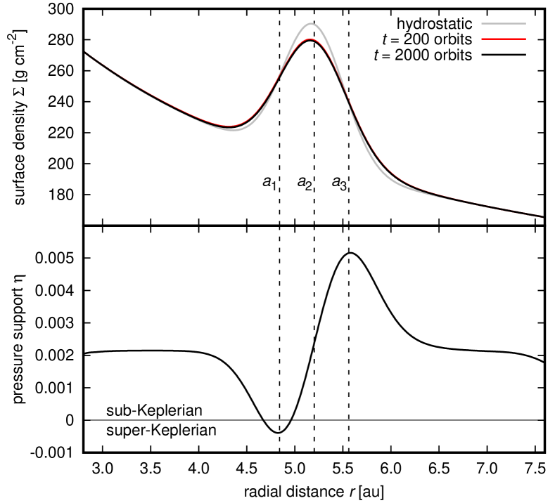
Figure 1: Top: Radial profile of the gas surface density $\Sigma$ after the hydrostatic relaxation (grey curve), after 200 orbits of the hydrodynamic relaxation (red curve), and at the end of the hydrodynamic relaxation (black curve). Bottom: Radial profile of the pressure support parameter $\eta$ in the relaxed disc. In both panels, vertical dashed lines mark the semi-major axes of planets considered in this work, $a=4.84$, $5.2$, and $5.56\,\mathrm{au}$. The horizontal $\eta=0$ line in the bottom panel separates the regimes of sub-Keplerian ($\eta>0$) and super-Keplerian ($\eta<0$) orbital velocities of the gas.

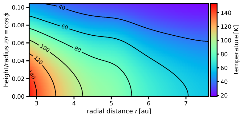
Figure 2: Gas temperature $T$ in the vertical plane of the relaxed disc before planet insertion. Black curves depict several temperature isocontours.

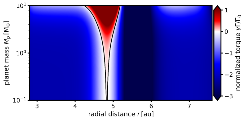
Figure 3: Estimate of the normalized gas-driven torque $\gamma\Gamma/\Gamma_{0}$ as a function of the planetary mass $M_{\mathrm{p}}$ and radial distance $r$ based on the formulae of Jiménez & Masset (2017), i.e. in the absence of thermal torques. Black isocontours mark the zero-torque locations; planets are expected to become trapped at the outer black curve where the predicted migration is convergent.

3.1 Relaxed disc

Fig. 1 (top panel) shows the radial profiles of the gas surface density $\Sigma$ obtained during the relaxation towards the thermodynamic equilibrium. Starting from our hydrostatic estimate, the bump amplitude slightly decreases and the bump edges undergo minor spreading over the first 200 dynamical time-scales of the hydrodynamic relaxation. Afterwards, the red and black curves are difficult to distinguish from one another and the profile remains almost unchanged.

Pressure bumps are typically characterized by the variation of the pressure support that a gas parcel feels while orbiting in the disc. We computed the pressure support parameter in the midplane (e.g. Nakagawa et al., 1986)

$$\eta=-\frac{1}{2}\left(\frac{H}{r}\right)^{2}\frac{\partial\log P}{\partial\log r}\,,$$ (9)

where $H$ is the non-isothermal pressure scale height that relates to the sound speed $c_{\mathrm{s}}=\sqrt{\gamma P/\rho}$ and the local Keplerian frequency $\Omega_{\mathrm{K}}=\sqrt{GM_{\star}/r^{3}}$ as $H=c_{\mathrm{s}}/(\sqrt{\gamma}\Omega_{\mathrm{K}})$. If $\eta>0$, the gas parcel orbits at a sub-Keplerian velocity. If, on the other hand, $\eta<0$, the gas parcel becomes super-Keplerian. Fig. 1 (bottom panel) indicates that $\eta\simeq 0.002$ away from the pressure bump, the maximum value of $\eta\simeq 0.005$ is reached roughly in the outer half of the surface density peak, and the minimum value of $\eta\simeq-4\times 10^{-4}$ is reached in the inner half of the $\Sigma$ peak.

In Fig. 2, we show the gas temperature $T$ in the vertical plane of the disc. The vertical temperature stratification is rather steep, as expected for a disc dominated by the viscous heating, and it is apparent that the bump does not have a strong influence on $T$. The bump only slightly flattens the radial temperature gradient, which results in the leveling of isocontours with the horizontal axis near 5 au in Fig. 2.

3.2 Bump parameters and the migration trap

The span of possible parameters characterizing pressure bumps in protoplanetary discs is largely unconstrained because the physics of these bumps is still a subject of intensive research. We choose the bump position $r_{\mathrm{b}}=5.2\,\mathrm{au}$ to tie our study of planet migration to previous works (Benítez-Llambay et al., 2015; Eklund & Masset, 2017). The Gaussian width $w_{\mathrm{b}}=0.32\,\mathrm{au}\simeq 1.5H$ is chosen to ensure that the bump remains Rossby-stable (wider than $H$; Lovelace et al., 1999; Dullemond et al., 2018). Regarding the bump amplitude $A_{\mathrm{b}}=1.45$, it is kept rather small but large enough to facilitate the existence of (i) a radial interval of super-Keplerian gas rotation and (ii) a migration trap in the absence of thermal torques, even for planets with very low masses. Point (i) is fulfilled based on Fig. 1 and point (ii) is proven in the following paragraph. As such, our bump can be interpreted to be close to the lower limit of $A_{\mathrm{b}}$ and $w_{\mathrm{b}}$ (while satisfying all of the above-mentioned requirements). Larger values of $A_{\mathrm{b}}$ and $w_{\mathrm{b}}$ are not ruled out by our study.

To verify that the pressure bump would act as a migration trap in the absence of thermal torques, we applied the torque formulae of Jiménez & Masset (2017) to our disc model and constructed the migration map shown in Fig. 3. According to the obtained result, low-mass planets would migrate inwards due to the dominance of the Lindblad torque in the majority of the disc (Tanaka et al., 2002). However, there is indeed a narrow interval of radii for which the disc torque would become positive due to a boost of the corotation torque (red colour in Fig. 3) and the planets would experience outward migration (Masset et al., 2006). At the outer edge of the red-coloured region, there is the zero-torque radius that would act as a migration trap in the pressure bump.

Having analyzed the disc properties and their influence on the Lindblad and corotation torques, we specify three values of interest for the planetary semi-major axes $a$. Our fiducial value is $a_{1}=4.84,\mathrm{au}$ and it is marked in Fig. 1 with the innermost vertical dashed line. At this disc location, the planet starts within the minimum of $\eta$ and at the same time, it finds itself within the V-shaped region of outward migration in Fig. 3. The second semi-major axis of interest is $a_{2}=5.2\,\mathrm{au}$ (middle dashed line in Fig. 1) for which the planet is close to the maximum of the surface density peak while $\eta$ is rather similar to the background unperturbed value. Finally, we choose $a_{3}=5.56\,\mathrm{au}$ (outermost dashed line in Fig. 1) as a counterpart to $a_{1}=4.84\,\mathrm{au}$ because it overlaps with the maximum of $\eta$.

3.3 Characteristic scales

The linear perturbation theory of thermal torques (Masset, 2017) argues that the thermal disturbance near a luminous planet has a characteristic length-scale

$$\lambda_{\mathrm{c}}=\sqrt{\frac{\chi}{(3/2)\Omega_{\mathrm{K}}\gamma}}\,,$$ (10)

where $\chi$ is the thermal diffusivity. Recent high-resolution simulations of inviscid discs with thermal diffusivity (Chametla & Masset, 2021; Velasco Romero et al., 2022) have demonstrated that the numerical convergence of thermal forces depends on the resolution and requires at least 10 cells per $\lambda_{\mathrm{c}}$, or $l/\lambda_{\mathrm{c}}=0.1$ where $l$ is the cell size.

In order to verify that our resolution is sufficient, we calculate the thermal diffusivity due to radiation diffusion in an optically thick medium as (Kley et al., 2009; Bitsch & Kley, 2011)

$$\chi=\frac{16\gamma(\gamma-1)\sigma T^{4}}{3\kappa(\rho H\Omega_{\mathrm{K}})^{2}}\,,$$ (11)

and, at $a_{1}=4.84\,\mathrm{au}$, we obtain $\chi=3.82\times 10^{15}\,\mathrm{cm}^{2}\,\mathrm{s}^{-1}$ and $\lambda_{\mathrm{c}}=0.02\,\mathrm{au}=0.1H$. Using the quadrant grid in the azimuth and the resolution specified in Table 1, we reach $l_{r}/\lambda_{\mathrm{c}}=0.09$, $l_{\theta}/\lambda_{\mathrm{c}}=0.09$, and $l_{\phi}/\lambda_{\mathrm{c}}=0.2$, where $l_{r,\theta,\phi}$ are the lengths of cell interfaces along the respective spherical coordinates. Therefore, the thermal disturbance is well resolved in the radial and azimuthal directions and only slightly under-resolved in the vertical direction, which we consider a reasonable compromise.

Additionally, Type I migration critically depends on the resolution of the half-width of the horseshoe region $x_{s}$ (Paardekooper et al., 2011; Jiménez & Masset, 2017), which influences the accuracy of the horseshoe drag (Ward, 1991; Masset, 2001; Baruteau & Masset, 2013). The minimal requirement for radiative discs is to resolve $x_{s}$ by 4 cells (Lega et al., 2014). For the lowest planetary mass that we shall consider in the following (see Table 2 for the range of parameters varied in our simulations), that is $M_{\mathrm{p}}=0.1\,M_{\earth}$, we have $(7,7,3)$ cells per $x_{s}$ in the $(r,\theta,\phi)$ directions. For $M_{\mathrm{p}}=1\,M_{\earth}$, we have $(21,21,10)$ cells per $x_{s}$, respectively. For completeness, let us remark the resolution of the Hill radius $R_{\mathrm{H}}$; we have $(12,12,6)$ cells per $R_{\mathrm{H}}$ for the Mars-mass planet and $(26,26,12)$ cells per $R_{\mathrm{H}}$ for the Earth-mass planet.

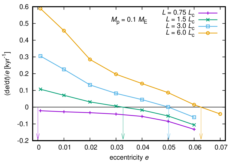
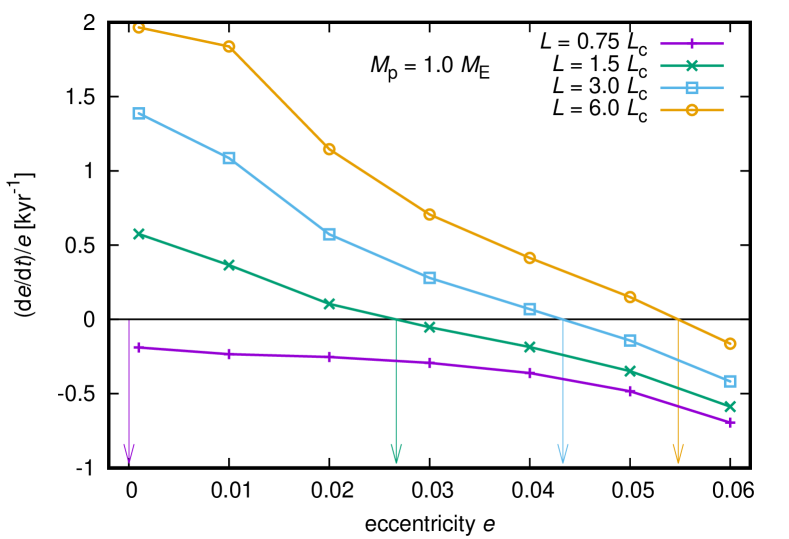
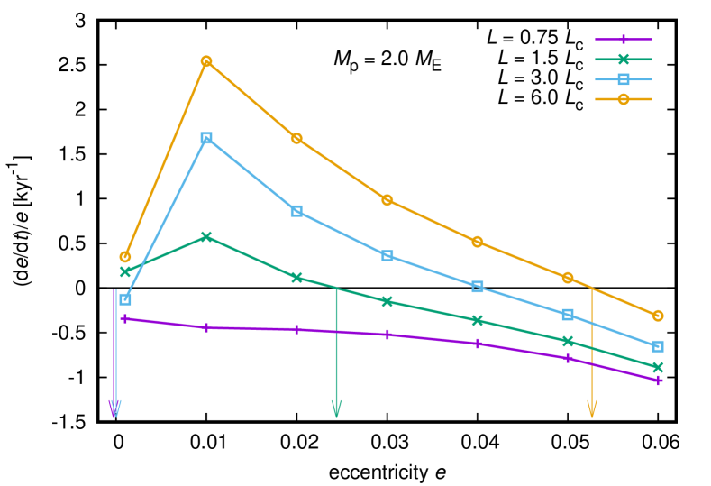
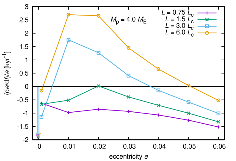
Figure 4: Eccentricity evolution rate $\dot{e}/e$ as a function of the initial orbital eccentricity $e$. Each panel summarizes simulations for a different planetary mass $M_{\mathrm{p}}$, as represented by the labels. Points and coloured segmented lines distinguish different values of the accretion luminosity $L$ as specified in the legend. Using corresponding colours, the vertical arrows mark the equilibrium eccentricity $e_{\mathrm{eq}}$ that the planets would asymptotically reach if they were evolving from a circular orbit at the given value of $L$. The horizontal zero line separates the regimes of eccentricity driving, $\dot{e}/e>0$, and damping, $\dot{e}/e<0$. Clearly, non-zero $e_{\mathrm{eq}}$ is reached in a substantial part of our parameter space. The case for $M_{\mathrm{p}}=0.5\,M_{\earth}$ is given in Fig. 13. We note that planets start migrating from $a_{1}=4.84\,\mathrm{au}$, i.e. from the minimum of $\eta$ (Fig. 1).

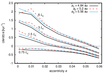
Figure 5: Eccentricity evolution rate $\dot{e}/e$ as a function of $e$ for $M_{\mathrm{p}}=1\,M_{\earth}$ migrating from different initial semi-major axes: $a_{1}=4.84$ (black solid curve), $a_{2}=5.2$ (dashed red curve), and $a_{3}=5.56\,\mathrm{au}$ (blue solid curve). The labels mark individual sets of curves with the respective value of $L$. For a given $L$, the curves are rather similar and therefore, $e_{\mathrm{eq}}$ is nearly independent of the initial position of the planet relative to the pressure bump.

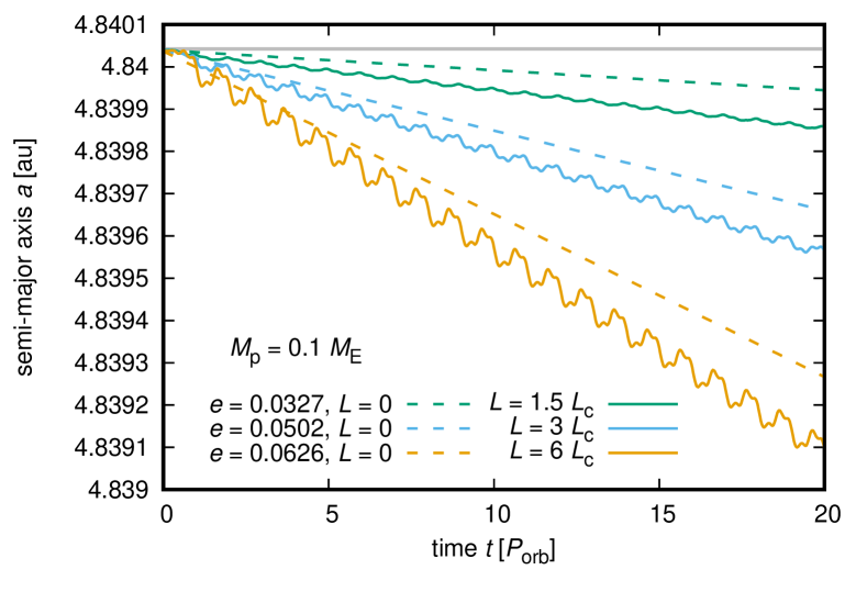
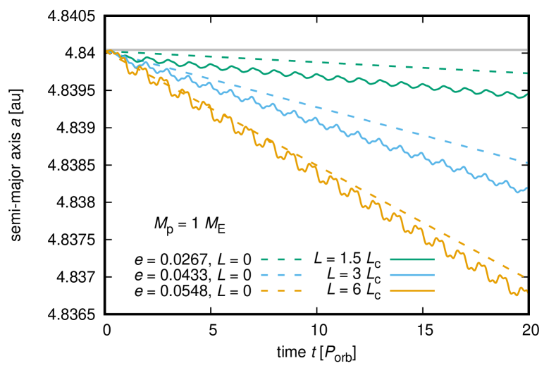
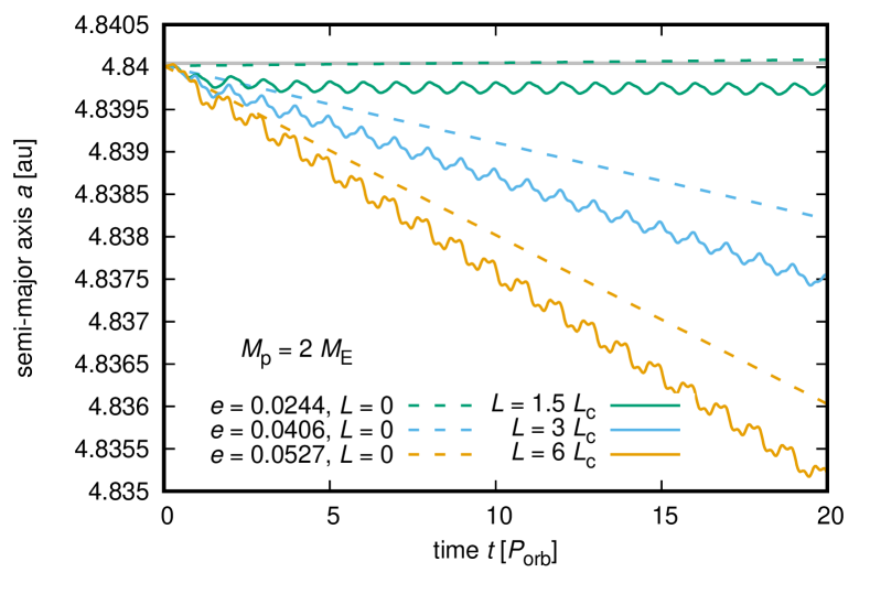
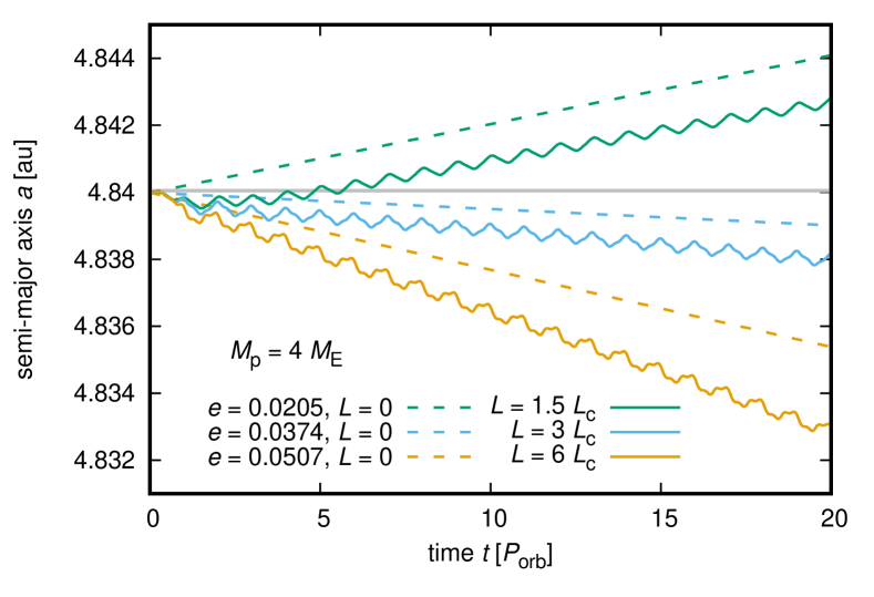
Figure 6: Temporal evolution of the semi-major axis $a$ for planets of different masses (see the labels of individual panels) in the headwind-dominated regime of thermal torques. Solid curves follow the migration of luminous planets starting at non-zero eccentricities $e$ for which $\dot{e}=0$ (Fig. 4). The values of $e$ and $L$ are given in the plot legend. We remind the reader that the values of $e$ represent $e_{\mathrm{eq}}$ for all luminous cases with the exceptions of $M_{\mathrm{p}}=4\,M_{\earth}$ and $M_{\mathrm{p}}=2\,M_{\earth}$, $L=3\,L_{\mathrm{c}}$. Dashed curves are the expected migration tracks for non-luminous planets at the same $e$ (they were obtained by analyzing the power of disc-driven forces affecting a planet in a fixed eccentric orbit). The horizontal gray line represents the initial semi-major axis. For both luminous and non-luminous planets, the change in the migration rate (slope) is mostly driven by the change in the eccentricity, not by a modification of thermal torques themselves. The reader is referred to Fig. 13 for $M_{\mathrm{p}}=0.5\,M_{\earth}$.

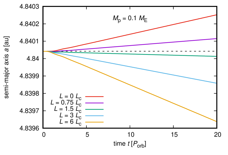
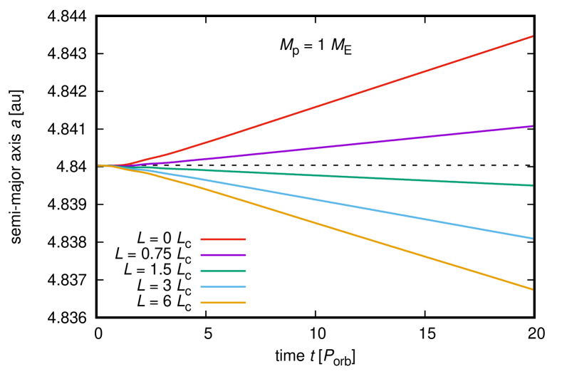
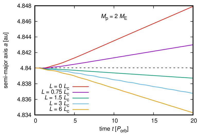
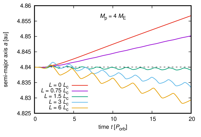
Figure 7: Evolution of the semi-major axis $a$ for planets starting at $a_{1}$ and $e=0$ (circular planets orbiting near the minimum of $\eta$). Individual panels are labelled with the planetary masses $M_{\mathrm{p}}$; the curves are coloured according to the luminosity of the planet $L$ (see the plot legend). Unlike in typical sub-Keplerian discs, here the shear-dominated regime of thermal torques facilitates inward migration with increasing $L$. The reader is referred to Fig. 13 for $M_{\mathrm{p}}=0.5\,M_{\earth}$.

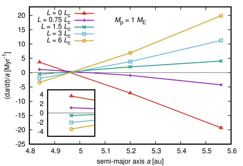
Figure 8: Evolution rate of the semi-major axis as a function of the position with respect to the pressure bump for $M_{\mathrm{p}}=1\,M_{\earth}$. The planet starts at $e=0$ and thermal torques operate in the shear-dominated regime. Different points and colours represent different luminosities of the planet, as specified in the plot legend. The inset shows an enlarged detail of measurements at $a_{1}$. We point out that the influence of thermal torques on the resulting migration rate is reversed at $a_{1}=4.84\,\mathrm{au}$ compared to $a_{2}=5.2$ and $a_{3}=5.56\,\mathrm{au}$ due to the variations of the background pressure support.

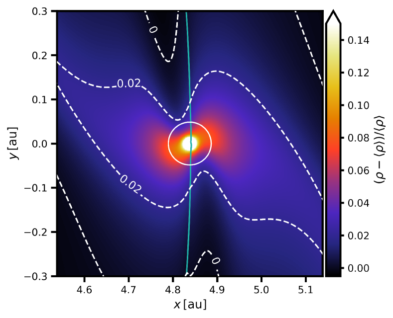
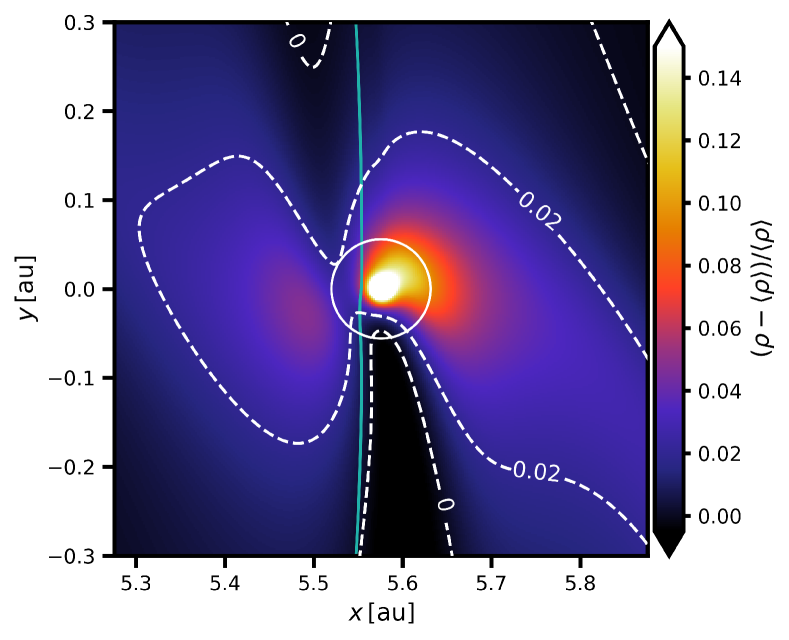
Figure 9: Perturbation of the gas density $\rho$ relative to the azimuthally-averaged gas density $\langle\rho\rangle$ in the disc midplane. The planet with $M_{\mathrm{p}}=1\,M_{\earth}$ is positioned in the centre of each panel and in the inertial frame, it would orbit in the $y>0$ direction. Left: Situation at $a_{1}$ where the disc is super-Keplerian. Right: Situation at $a_{3}$ where the disc is strongly sub-Keplerian. The white circle marks the Hill sphere, the light green curve marks the position where the disc material corotates with the planet ($v_{\theta}=0$ with respect to the planet), and white dashed curves are selected isocontours. The closeness of a given isocontour to the Hill sphere can be used as a measure of the asymmetry between the two underdense lobes (isocontours near a deeper lobe are prolated closer to the planet). The inner leading lobe dominates at $a_{1}$ while the outer trailing lobe dominates at $a_{3}$. The thermal torque is negative at $a_{1}$ while it is positive at $a_{3}$.

Parameter	Notation/Scaling	Values
Planet mass	$M_{\mathrm{p}}/M_{\earth}$	$0.1,0.5,1,2,4$
Semi-major axis	$a/\mathrm{au}$	$4.84,5.2,5.56$
Luminosity	$L/L_{\mathrm{c}}$	$0,0.75,1.5,3,6$
Eccentricity	$e$	$(0,0.1,1,2,3,4,5,6)\times 10^{-2}$

Table 2: Parameter space explored in our simulations. The respective combinations of parameters are specified in individual sections. We remind the reader that $L_{\mathrm{c}}$ itself is a function of $M_{\mathrm{p}}$.

3.4 Eccentricity excitation of luminous planets in the super-Keplerian bump region

Thermal forces can in principle change both the semi-major axis $a$ and eccentricity $e$ of migrating planets. Therefore, to evaluate the migration of planets near pressure bumps, it is necessary to establish whether $e$ can become non-zero and if so, what is the equilibrium value $e\rightarrow e_{\mathrm{eq}}$ for which the eccentricity driving and damping are balanced.

We start our investigation at $a_{1}=4.84\,\mathrm{au}$ where the region of outward (or stalled) migration is expected to exist and planets should become trapped close to it (Fig. 3). We explore the parameter space of planetary masses $M_{\mathrm{p}}/M_{\earth}=(0.1,0.5,1,2,4)$, initial eccentricities $e(t=0)=(0.1,1,2,3,4,5,6)\times 10^{-2}$, and luminosities $L/L_{\mathrm{c}}=(0.75,1.5,3,6)$ that are scaled using the critical luminosity (Masset, 2017)

$$L_{\mathrm{c}}=\frac{4\pi GM_{\mathrm{p}}\chi\rho}{\gamma}\,.$$ (12)

The critical luminosity is expected to separate the regimes of eccentricity damping and driving for $L<L_{\mathrm{c}}$ and $L>L_{\mathrm{c}}$, respectively (Masset & Velasco Romero, 2017; Fromenteau & Masset, 2019; Velasco Romero et al., 2022; Cornejo et al., 2023). By plugging equation (12) into (4), one finds that the mass doubling time necessary to reach $L_{\mathrm{c}}$ scales as $\tau\propto M_{\mathrm{p}}^{2/3}$. For our span of planetary masses $M_{\mathrm{p}}/M_{\earth}=(0.1,0.5,1,2,4)$, the luminosity becomes equal to $L_{\mathrm{c}}$ for $\tau\simeq(36,105,166,264,419)\,\mathrm{kyr}$, respectively. These values of $\tau$ are substantially larger with respect to our typical integration times, which cover several planetary orbits. It is therefore appropriate to keep the planetary masses fixed in our simulations and consider the luminosity as a free parameter. Since our high-resolution radiative simulations are numerically demanding and the number of parameters is relatively large, we start by performing simulations over $5$ orbital periods of the planet (with a few exceptions specified below). Planets are smoothly introduced in the simulations by ramping $M_{\mathrm{p}}$ from zero to its parametric value over the first orbital time-scale.

Fig. 4 shows the eccentricity evolution rate $\dot{e}/e$ as a function of the initial orbital eccentricity for all our parameters (see Fig. 13 for $M_{\mathrm{p}}=0.5\,M_{\earth}$). The time derivative of the eccentricity $\dot{e}$ was obtained by fitting a linear function to the time series of $e(t)$ that were recorded during our simulations. The fit was performed over the last three orbits and $\dot{e}$ was determined from its slope. For several cases with the lowest eccentricity $e=10^{-3}$, the behaviour of $e(t)$ was deviating from a linear trend on the time-scale of three orbits. We thus extended these specific cases to twenty orbital periods and we performed the linear fit over the last eighteen orbits.

Similarly to Eklund & Masset (2017) or Velasco Romero et al. (2022), Fig. 4 allows us to find the equilibrium asymptotic eccentricity $e_{\mathrm{eq}}$ that the planets would reach. If $\dot{e}<0$ for $e=10^{-3}$, we take $e_{\mathrm{eq}}=0$. Such cases represent planets that, when starting on circular orbits, feel the eccentricity damping straightaway, which prevents them from any eccentricity growth. If, on the other hand, $\dot{e}>0$ for $e=10^{-3}$, we find $e_{\mathrm{eq}}$ by applying linear interpolation to our measurements and identifying the point where $\dot{e}=0$. In these cases, planets starting at $e<e_{\mathrm{eq}}$ experience eccentricity driving while planets starting at $e>e_{\mathrm{eq}}$ experience eccentricity damping. Equilibrium eccentricities $e_{\mathrm{eq}}$ are marked by arrows in Fig. 4 and summarized in Table 3.

We see that the planets remain circular as long as their luminosity is sub-critical. Once the luminosity becomes super-critical, $e_{\mathrm{eq}}$ reaches values of the order of $h=H/r$ (Chrenko et al., 2017) in most cases. As for other trends, larger $L$ implies larger $e_{\mathrm{eq}}$ for fixed $M_{\mathrm{p}}$, while smaller $M_{\mathrm{p}}$ implies larger $e_{\mathrm{eq}}$ for fixed $L$, in good agreement with Velasco Romero et al. (2022). In the case with $M_{\mathrm{p}}=2\,M_{\earth}$ and $L=3\,L_{\mathrm{c}}$, as well as for all cases with $M_{\mathrm{p}}=4\,M_{\earth}$, we find $e_{\mathrm{eq}}=0$ even for the super-critical $L$. We attribute this behaviour to the non-linearities that arise for increasing planetary masses for which the advective redistribution of hot gas close to the planet does not reach a steady state (Chrenko & Lambrechts, 2019). These cases are covered in greater detail in Section 3.7. For $M_{\mathrm{p}}\leq 1\,M_{\earth}$, however, we conclude that $L_{\mathrm{c}}$ (that was originally derived from the linear perturbation theory in discs with thermal diffusion; Masset, 2017) is a robust separation for the eccentricity damping and excitation even in 3D radiative discs.

$L$	$e_{\mathrm{eq}}$ for $M_{\mathrm{p}}/M_{\earth}=$
	0.1	0.5	1	2	4
0.75 $L_{\mathrm{c}}$	0	0	0	0	0
1.5 $L_{\mathrm{c}}$	0.033	0.029	0.027	0.024	0
3 $L_{\mathrm{c}}$	0.05	0.046	0.043	0	0
6 $L_{\mathrm{c}}$	0.063	0.057	0.055	0.053	0

Table 3: Equilibrium eccentricities $e_{\mathrm{eq}}$ (columns 2–6) for various planetary masses $M_{\mathrm{p}}$ and luminosities $L$ (column 1). For $L>L_{\mathrm{c}}$, planets acquire orbits with substantial eccentricities in the majority of our parameter space.

3.5 Headwind-dominated regime

Section 3.4 reveals that $e_{\mathrm{eq}}\sim h$ for the majority of our parameter space. These relatively large eccentricities place the planets firmly to the headwind-dominated regime of thermal torques (Eklund & Masset, 2017) for which the two-lobed density perturbation (Benítez-Llambay et al., 2015) becomes replaced by a single hot trail (Chrenko et al., 2017). Here, we focus on the headwind-dominated regime in greater detail.

As a first step, we need to establish whether the magnitude of eccentricity excitation from Fig. 4 is universal or rather dependent on the local conditions within the pressure bump. To this point, we repeated the measurement from Fig. 4 for $M_{\mathrm{p}}=1\,M_{\earth}$ but this time we placed the planet at initial semi-major axes $a_{2}=5.2$ and $a_{3}=5.56\,\mathrm{au}$ to investigate $\dot{e}$ at the bump centre and at the maximum of $\eta$, respectively.

Fig. 5 compares the eccentricity evolution rate at different locations in the pressure bump. Although we detect marginal differences at very low $e$, the values obtained at fixed $L$ are rather similar, which makes them independent of $a$. Therefore, the ability of a planet to reach the headwind-dominated regime with non-zero $e_{\mathrm{eq}}$ does not depend on its position with respect to the pressure bump. Once the planet develops non-zero $e_{\mathrm{eq}}$ anywhere, it will tend to maintain it despite its radial migration.

Next, we explore the migration in the headwind-dominated regime. Focusing solely on $a_{1}$ again, we let the planets migrate using $e_{\mathrm{eq}}$ from Table 3 as their initial eccentricities. For the cases with $L\geq 1.5\,L_{\mathrm{c}}$ and $M_{\mathrm{p}}\geq 2\,M_{\earth}$ that exhibit $e_{\mathrm{eq}}=0$ in Table 3, we start from their largest $e$ that would lead to $\dot{e}=0$ in Fig. 4. The simulation time-scales for migrating planets are equal to 20 orbital periods.

Fig. 6 (solid curves) shows the resulting temporal evolution of semi-major axes. Clearly, planets with super-critical luminosities often abandon the outward migration predicted by Fig. 3 and they predominantly switch to inward migration. We only detect stalled migration for $M_{\mathrm{p}}=2\,M_{\earth}$ and $L=1.5\,L_{\mathrm{c}}$, outward migration for $M_{\mathrm{p}}=4\,M_{\earth}$ and $L=1.5\,L_{\mathrm{c}}$, and we point out that the migration of $M_{\mathrm{p}}=0.1\,M_{\earth}$ is generally slow because of its very low mass (see the extent of the vertical axis in Fig. 6).

Since the inward migration becomes faster with increasing $L$, is is natural to ask whether this effect is somehow regulated by the thermal torques themselves or whether it is driven by the Lindblad and corotation torques operating at increased eccentricities. To find the answer, we performed simulations with non-luminous planets that are subject to cold thermal torques in radiative discs (Lega et al., 2014; Masset, 2017). We placed these planets on fixed eccentric orbits with the same span of $e$ as used for their luminous counterparts. The purpose of fixing the orbits is to prevent the eccentricity damping. To predict the migration outcome, we measured the torque $\Gamma$ and power $P$ exerted by the gravitational disc forces, then we averaged these values over the last ten orbital periods, and we estimated (e.g. Bitsch & Kley, 2010)

$$\frac{\dot{a}}{a}=\frac{2a}{GM_{\star}M_{\mathrm{p}}}P\,,$$ (13)

which expresses the evolution rate of the semi-major axis from the change in the orbital energy.

By integrating Equation (13), we obtained the dashed curves shown in Fig. 6. Focusing on the change in the slope of $a(t)$ curves, it becomes clear that the cases with $L=0$ exhibit the same change of slope with the increase of $e$ as the cases with $L\neq 0$. Although there is a small systematic offset between the $L=0$ and $L\neq 0$ curves, it does not seem to strongly depend on the actual value of $L$ (in contrast to Fig. 7 discussed later). Therefore, we obtain an important result: The actual migration rate for $e_{\mathrm{eq}}$ corresponding to the headwind-dominated regime is not controlled by thermal torques themselves, these are only responsible for keeping $e$ pumped up. Instead, the migration rate is controlled by the standard Lindblad and corotation torques. Since the latter experiences exponential quenching with increasing $e$ (Fendyke & Nelson, 2014), the inward migration in Fig. 6 becomes faster for larger $e$ as the Lindblad torque becomes more and more dominant.

The implications of this section are the following. The excitation of $e_{\mathrm{eq}}\sim h$ is a global effect independent of planet position in the disc and at this level of eccentricity, the migration is governed mostly by the Lindblad and corotation torques. Then, if a luminous planet is found to exhibit inward migration at $a_{1}$ where Fig. 3 predicts outward (or stalled) migration and where the corotation torque is the strongest, it will be subject to inward migration in our entire simulated disc because the corotation torque can only become weaker away from $a_{1}$ and the Lindblad torque is always negative. Hence, for the inward-migrating planets from Fig. 6, the migration trap at the pressure bump does not exist.

3.6 Shear-dominated regime

Let us now turn out attention to the migration at $e=0$ for which the thermal torques operate in the shear-dominated regime. This regime becomes important when $L<L_{\mathrm{c}}$ (Table 3), or when the behaviour of thermal torques becomes highly non-linear (e.g. for our case $M_{\mathrm{p}}=4\,M_{\earth}$), and we also expect that planets can temporarily evolve in this regime if they are born in circular orbit before having their $e$ excited.

We performed simulations of both cold and luminous planets ($L/L_{\mathrm{c}}=(0,0.75,1.5,3,6)$) evolving from $e=0$ and starting at three distinct positions $a_{1}$, $a_{2}$, and $a_{3}$ spread across the pressure bump. The simulations covered 20 orbital periods again. Fig. 7 depicts the migration tracks at $a_{1}$. The migration is outward, and thus in accordance with the migration map in Fig. 3, as long as $L<L_{\mathrm{c}}$ and we also find one case of stalled migration for $M_{\mathrm{p}}=4\,M_{\earth}$, $L=1.5\,L_{\mathrm{c}}$. For the remaining cases, however, the migration becomes directed inwards and surprisingly, its rate becomes faster with increasing $L$. This is in striking contrast to the usual behaviour of thermal torques in simple power-law discs (Benítez-Llambay et al., 2015) where increasing $L$ typically makes the migration tracks more and more outward.

To further highlight this finding, Fig. 8 shows the evolution rate of the semi-major axis $\dot{a}/a$ for $M_{\mathrm{p}}=1\,M_{\earth}$ at all three initial semi-major axes $a_{1}$, $a_{2}$, and $a_{3}$. The behaviour at $a_{1}$ is as described in the previous paragraph. The behaviour at $a_{2}$ and $a_{3}$ is antisymmetric, in a sense that the fastest inward migration (i.e. the most negative total torque) is found for $L=0$ and then it slows down and reverses as $L$ increases (i.e. the torque receives gradual positive boosts each time $L$ grows).

We infer that these trends are related to the local disc rotation and pressure support. The locations $a_{2}$ and $a_{3}$ have $\eta>0$ (Fig. 1) and the local rotation is sub-Keplerian. Therefore, the exact corotation between the disc material and the planet is offset inwards with respect to the planet and the resulting two-lobed underdensity is asymmetric because the disc shear is more efficient in advecting the hot gas into the outer lobe, trailing the orbital motion of the planet. Since $\eta$ is larger at $a_{3}$, so is the offset of the planet from the corotation and the thermal torques are more prominent compared to $a_{2}$. This is in accordance with Benítez-Llambay et al. (2015).

However, $\eta<0$ at $a_{1}$ (super-Keplerian rotation) and the same reasoning implies that the exact corotation is located outwards from the planet and the inner underdense lobe that leads the orbital motion of the planet will dominate over the outer one. In other words, the lack of gas ahead of the planet means that the planet will be robed of angular momentum by the gas trailing it. The total torque will therefore become more negative, which facilitates the shift towards inward migration found in Figs. 7 and 8 at the minimum of $\eta$.

As a verification of our claims, Fig. 9 shows the density perturbation in the disc midplane near an Earth-mass planet. The density perturbation $(\rho-\langle\rho\rangle)/\langle\rho\rangle$ is computed with respect to the azimuthal average $\langle\rho\rangle$. By tracing the isocontours, one can see that the excavation of the inner lobe is larger at $a_{1}$ (left panel in Fig. 9), while the outer lobe dominates at $a_{3}$ (right panel in Fig. 9). This asymmetry depends on where the disc material corotates with the planet, as indicated by the light green curve in Fig. 9. We point out that the dependence of thermal torques on the corotation offset has already been described in previous works (Benítez-Llambay et al., 2015; Masset, 2017; Chametla & Masset, 2021), however, the case when the corotation is located farther out with respect to the planet was not considered in detail or it was explicitly regarded as unrealistic (Benítez-Llambay et al., 2015). Here, instead, we demonstrate that the impact of such an outward corotation offset, which inherently occurs near pressure bumps (left panel in Fig. 9), can be substantial.

Before summarizing this section, let us also point out that while the evolution of the semi-major axes can be reverted depending on $\eta$, the eccentricity evolution rate is affected only weakly as we saw in Fig. 5. An extended analysis of this fact for the shear-dominated regime is provided in Appendix B.

The implications of this section are best inferred from Fig. 8, which reveals a radius of convergent migration (roughly at $4.95\,\mathrm{au}$) for $L<L_{\mathrm{c}}$ but leads to divergent migration for $L>L_{\mathrm{c}}$. Therefore, if planets with super-critical luminosities remain circular (which happens only for a limited subset of our parameter space), they are again expected to migrate away from the pressure bump. If these planets were to start at $a_{1}$, they could possible get trapped near $a\simeq 4.67\,\mathrm{au}$ where $\eta$ becomes positive again and thus we can expect another change in the sign of $\dot{a}$ (not explored in our Fig. 8). If these planets were to start at $a_{2}$ or $a_{3}$, they would migrate outwards.

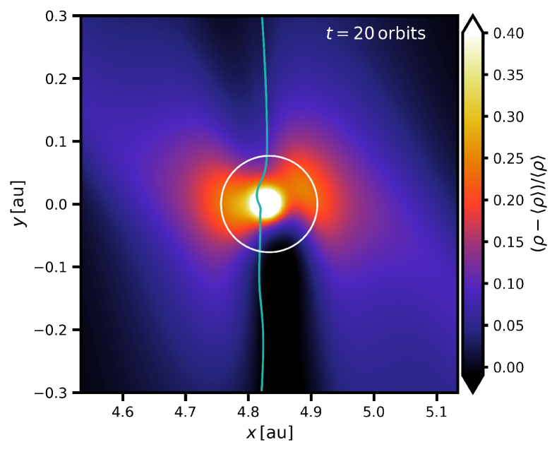
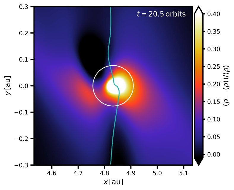
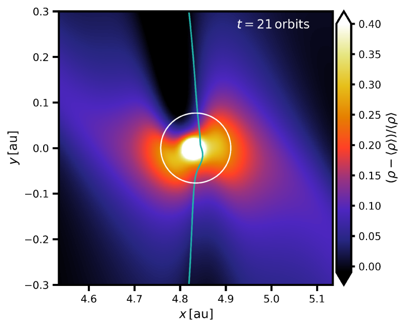
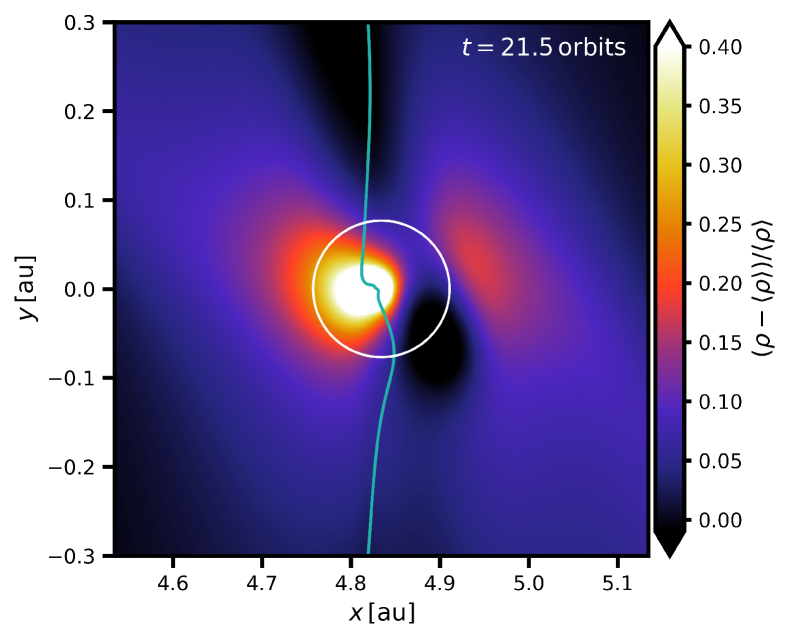
Figure 10: As in Fig. 9 but for $M_{\mathrm{p}}=4\,M_{\earth}$ at $a_{1}$ with $L=6\,L_{\mathrm{c}}$. The two rows cover two consecutive orbital cycles (individual panels are labelled with corresponding simulation times $t$). The fluctuations suggest that the circumplanetary flow never reaches a steady state, similarly to Chrenko & Lambrechts (2019).

3.7 Fluctuating thermal disturbance

When assessing the equilibrium eccentricities, we saw in Fig. 4 that while the planets with $M_{\mathrm{p}}\leq 1\,M_{\earth}$ exhibit an orderly and mildly decreasing dependence of $\dot{e}$ on $e$, our most massive planets exhibit a break near the smallest eccentricities. Consequently, these planets are capable of remaining circular even at super-critical luminosities (Table 3). Similarly, when focusing on the migration of these planets in the circular case, we saw that the semi-major axis evolution is accompanied by short-term oscillations that are best apparent for $M_{\mathrm{p}}=4\,M_{\earth}$ and $L\gtrsim 1.5\,L_{\mathrm{c}}$ (Fig. 7, bottom right).

By investigating the gas evolution for these peculiar cases, we found that they exhibit fluctuations of the thermal disturbance. These fluctuations were first reported in Chrenko & Lambrechts (2019) and they are driven by a complex reconfiguration of the 3D circumplanetary flow. An interesting fact is that while Chrenko & Lambrechts (2019) found the presence of these fluctuations in a setup with temperature-dependent disc opacities, here we obtain the same behaviour in a constant-opacity disc.

Fig. 10 shows the temporal evolution of the gas density perturbation for $M_{\mathrm{p}}=4\,M_{\earth}$ and $L=6\,L_{\mathrm{c}}$ during two orbits of the planet. At $t=20$ orbits (top left panel), the outer rear lobe dominates. After one half of the orbit (top right panel), the outer rear lobe shrinks while the inner front lobe becomes more pronounced. At $t=21$ orbits (bottom left panel), the inner front lobe dominates. The cycle returns to the beginning shortly after $t=21.5$ orbits (bottom right panel).

The realism of the fluctuating thermal disturbance is still somewhat unclear because Chrenko & Lambrechts (2019) showed that its occurrence is favoured in discs with vertically steep temperature gradients. Realistic protoplanetary discs that are stellar-irradiated have shallower vertical temperature gradients than discs heated purely by viscous friction (considered here), future work should therefore examine the occurrence of fluctuating thermal disturbances in stellar-irradiated discs as well. However, the fact that the fluctuations naturally appear in our constant-opacity setup with much better resolution than Chrenko & Lambrechts (2019) provides additional independent indication of their robustness.

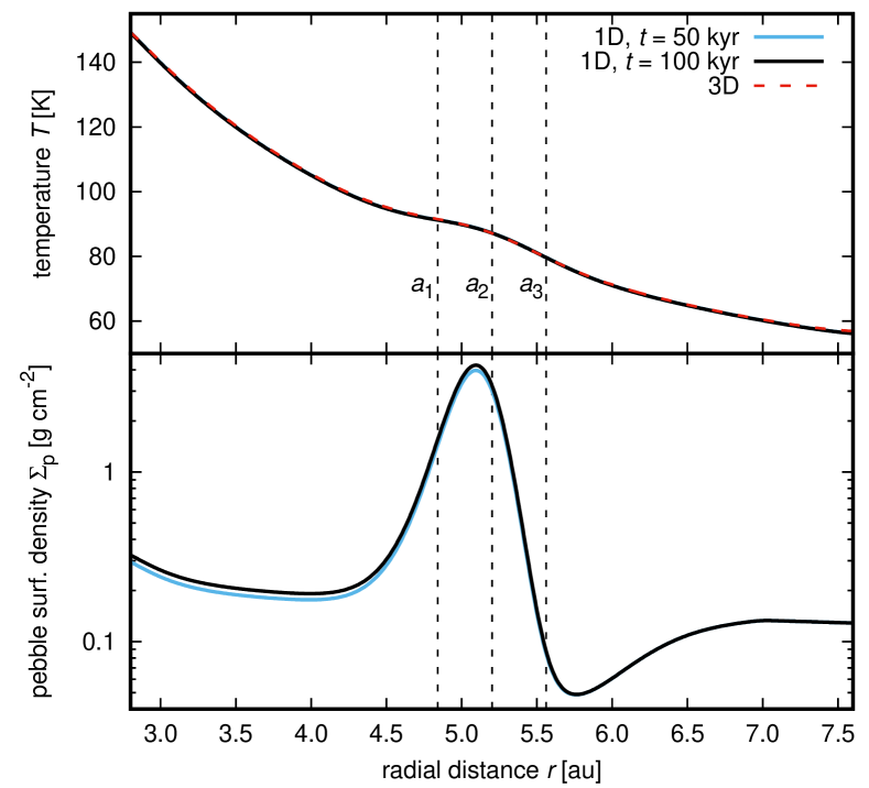
Figure 11: Radial profile of the gas temperature $T$ (top) and pebble surface density $\Sigma_{\mathrm{p}}$ (bottom) during the evolution (blue and black curves) of our bi-fluid 1D model. Red dashed curve in the top panel shows the equilibrium profile of our 3D disc (see Fig. 1) for reference. The vertical dashed lines mark the positions $a_{1}$, $a_{2}$, and $a_{3}$ used in our simulations with planets.

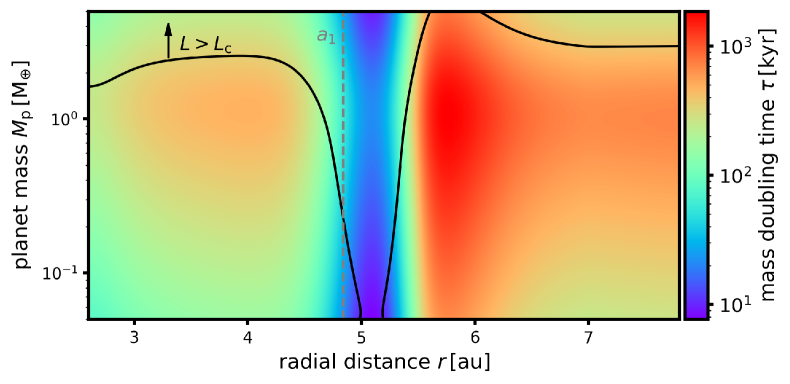
Figure 12: Mass doubling time $\tau$ due to pebble accretion as a function of the planet mass $M_{\mathrm{p}}$ and radial distance $r$ in the disc. The region above the solid black curve is where the luminosity of accreting planets becomes super-critical, $L>L_{\mathrm{c}}$. The vertical dashed line marks the location $a_{1}$. Planets are accreting pebbles with $\mathrm{St}=0.07$ and the pebble flux at the outer boundary is $10^{-4}\,M_{\earth}\,\mathrm{yr}^{-1}$.

3.8 Luminosity reached by pebble accretion

In previous sections, the luminosity $L$ of accreting planets was a free parameter unrelated to any physical process. The aim of this section is to determine the values of $L$ that can be reached by pebble accretion (Ormel & Klahr, 2010; Lambrechts & Johansen, 2012), which is thought to be a major accretion channel in many planet formation scenarios (e.g. Lambrechts et al., 2014; Bitsch et al., 2019; Venturini et al., 2020; Brož et al., 2021).

We constructed a simple model for a coupled evolution of gas and pebbles. We solved 2D vertically-integrated continuity and Navier-Stokes equations for a bi-fluid mixture of gas and pebbles using Fargo3D again and we additionally assumed axial symmetry, thus making the model effectively 1D. Gas and pebbles were aerodynamically coupled (e.g. Chametla & Chrenko, 2022) and the turbulent pebble diffusion was taken into account as well (Weber et al., 2019). To maintain the disc non-isothermal and thus comparable to our 3D model, we included a one-temperature gas energy equation in the form of Chrenko et al. (2017) while neglecting the stellar irradiation term. Unlike in Chrenko et al. (2017) (see equation 11 of that paper), we did not include any opacity correction in the vertical optical depth (Hubeny, 1990). The disc parameters were the same as in the case of our 3D disc.

The 1D simulation was started by an iterative hydrostatic relaxation similar to Section 2.1. Once the gas temperature equilibrated, we added the pebble component by assuming a constant pebble flux $\dot{M}_{\mathrm{F}}=10^{-4}\,M_{\earth}\,\mathrm{yr}^{-1}$ through the disc:

$$\Sigma_{\mathrm{p}}=-\frac{\dot{M}_{\mathrm{F}}}{2\pi rv_{r,\mathrm{p}}}\simeq\frac{\dot{M}_{\mathrm{F}}}{4\pi r^{2}\mathrm{St}\eta\Omega_{\mathrm{K}}}\,,$$ (14)

where $\Sigma_{\mathrm{p}}$ is the initial pebble surface density, $v_{r,\mathrm{p}}$ is the radial drift velocity of pebbles and $\mathrm{St}=0.07$ is the Stokes number (dimensionless stopping time) of pebbles (Nakagawa et al., 1986). For the sake of pebble initialization, we used $\eta$ corresponding to a bump-free disc (because Equation 14 would lead to $\Sigma_{\mathrm{p}}<0$ for $\eta<0$ inside the bump, which would be unphysical). The value of $\mathrm{St}$ was derived in a bump-free disc again, assuming that the dominant physical radius of pebbles is drift-limited (Lambrechts & Johansen, 2014; Chrenko et al., 2017). We evolved the disc for $8,500$ orbital time-scales, which evaluates roughly to $t\simeq 100\,\mathrm{kyr}$. To maintain the pebble flux entering the disc uniform, we damped $\Sigma_{\mathrm{p}}$ to its initial value close to the outer boundary.

The result of our simulation is given in Fig. 11. First, the top panel demonstrates that the temperature profile of the 1D disc is indeed comparable to our more advanced 3D model. Second, the bottom panel shows the radial profile of $\Sigma_{\mathrm{p}}$ and reveals that our parametrization of the pressure bump does not create a perfect barrier to the pebble flux. This is because the region of $\eta<0$ is relatively narrow (see Fig. 1) and thus, once the mass loading of the bump by pebbles becomes sufficient, the pebbles start to penetrate the bump by means of turbulent diffusion. Due to the latter, the radial flux of pebbles inwards from the bump remains non-zero. Since $\Sigma_{\mathrm{p}}$ is not evolving substantially between $t=50$ and $100\,\mathrm{kyr}$, it is clear that an equilibrium state was reached.

Having the knowledge of $\Sigma_{\mathrm{p}}$, we calculated the pebble accretion rate for a range of planetary masses across the disc. The calculation followed the recipe of Liu & Ormel (2018) that was reformulated by Jiang & Ormel (2023) for the environment of pressure bumps. We neglected any vertical stirring of pebbles (and thus also the 3D regime of pebble accretion) and we assumed circular orbits of planets. The results are shown in Fig. 12 in terms of the mass doubling time $\tau$. Clearly, the accumulation of pebbles at the bump boosts the accretion efficiency (shortens $\tau$) and the growth of planets can become rapid. In the light of our study, however, we can see that growing planets easily exceed the critical luminosity $L_{\mathrm{c}}$. At $a_{1}$, this happens for $M_{\mathrm{p}}\simeq 0.2\,M_{\earth}$. Consequently, planets with $M_{\mathrm{p}}\gtrsim 0.2\,M_{\earth}$ would undergo eccentricity excitation, they would enter the headwind-dominated regime, and they would start migrating inwards.

4 Discussion

4.1 On the viability of model parameters

The full parameter space of our model is extensive and we thus only focused on exploring several specific dependencies. We have already explained our rationale behind selecting parameters for the pressure bump and planetary luminosity in Sections 3.2 and 3.4, respectively. However, it is important to discuss the remaining model parameters, namely, the opacity $\kappa=1\,\mathrm{cm}^{2}\,\mathrm{g}^{-1}$ and the kinematic viscosity $\nu=10^{15}\,\mathrm{cm}^{2}\,\mathrm{s}^{-1}$. These values were adopted from Eklund & Masset (2017) in order to establish a connection between our study and prior research. Nevertheless, one should bear in mind that $\kappa$ and $\nu$ can vary over orders of magnitude in realistic protoplanetary discs.

For less opaque protoplanetary discs, the efficiency of thermal torques decreases, as numerically demonstrated by Benítez-Llambay et al. (2015) and analytically shown by Masset (2017). This torque reduction occurs because a lower opacity leads to a larger thermal diffusivity (Equation 11) while the hot thermal torque component scales as $\propto$$\chi^{-3/2}$ in the linear regime. In the light of our study, however, we must also ask how the eccentricity excitation is affected. By utilizing the results from linear theory, we can roughly estimate that the eccentricity will grow as long as (i) the response time of the thermal driving $t_{\mathrm{th}}$ is shorter than the time-scale of wave-induced damping $t_{\mathrm{wave}}$ (Tanaka & Ward, 2004) and (ii) the luminosity remains super-critical. Both of these conditions are dependent on $\chi$ and thus influenced by $\kappa$. Regarding (i), Fromenteau & Masset (2019) found

$$\frac{t_{\mathrm{th}}}{t_{\mathrm{wave}}}=\sqrt{\frac{\pi}{2}}\frac{1}{\gamma\left(\gamma-1\right)}\frac{\lambda_{\mathrm{c}}}{H}\,,$$ (15)

and we recall that $\lambda_{\mathrm{c}}=0.1H$ in our model. To prevent the eccentricity growth of luminous planets born in circular orbits, $\kappa$ would need to decrease sufficiently to expand $\lambda_{\mathrm{c}}\propto\sqrt{\chi}$ by an order of magnitude. Nevertheless, determining the critical value of $\kappa$ at which the wave-induced damping dominates is not straightforward because not only $\chi\propto\kappa^{-1}$, but also $\chi\propto T^{4}$ and we expect that the equilibrium temperature profile of a disc with lower opacity would be cooler. Regarding (ii), lower $\kappa$ (and consequently larger $\chi$) would elevate the critical luminosity threshold $L_{\mathrm{c}}$. In other words, larger accretion rates (lower mass doubling times $\tau$) would be required to initiate the eccentricity growth.

To assess whether the value of $\kappa=1\,\mathrm{cm}^{2}\,\mathrm{g}^{-1}$ is appropriate for the studied disc region, we compared it with the Rosseland opacities based on the DIANA standard for the dust composition (Woitke et al., 2016) within the temperature range of our disc. Appendix C and Fig. 15 show that these more detailed opacities are similar to $\kappa=1\,\mathrm{cm}^{2}\,\mathrm{g}^{-1}$ at the radial positions $a_{1}$–$a_{3}$, which we have considered as the initial locations for the planets. We admit, however, that the planets themselves are surrounded by temperature peaks when they release the accretion heat (for instance, $M_{p}=1\,M_{\earth}$ at $L=3\,L_{\mathrm{c}}$ exhibits a temperature peak exceeding $200\,\mathrm{K}$) and our constant-opacity model is certainly a simplification within these local temperature maxima.

Concerning the viscosity, the value of $\nu=10^{15}\,\mathrm{cm^{2}}\,\mathrm{s}^{-1}$ translates to the Shakura-Sunyaev viscosity (Shakura & Sunyaev, 1973) of $\alpha\simeq 3.5$–$4\times 10^{-3}$ across the pressure bump, which is relatively large and requires a substantial level of turbulent stress to operate. Such a stress might be difficult to achieve because a hydrodynamic turbulence is typically weaker (e.g. Nelson et al., 2013; Klahr et al., 2018; Pfeil & Klahr, 2019) and a magneto-hydrodynamic turbulence in the midplane at several au is likely to be suppressed (e.g. Turner et al., 2014; Lesur et al., 2022). At lower and vanishing viscosities, we think that the response of planets to the thermal perturbation shown in our study remains valid because Velasco Romero et al. (2022) reported similar eccentricity evolution in models of inviscid power-law discs with thermal diffusion. Additional effects, however, can be expected in discs with pressure bumps because in the low-viscosity limit, embedded planets might perturb the bumps more prominently and they might even destabilize them. This problem is left for future work.

4.2 Implications for planet formation at pressure bumps

Pressure bumps have been proposed as efficient sites of planet accretion in several recent works (Section 1). However, if the accretion is indeed efficient, it is likely that the accreting planets will exceed the critical luminosity and begin experiencing eccentricity excitation due to thermal driving. Our simulations robustly demonstrate that the eccentricities become non-zero for the majority of considered planetary masses, beginning with those as small as Mars-sized embryos. Such eccentric planets experience inward migration because they lose the support of the corotation torque. Planets with $M_{\mathrm{p}}\simeq 4\,M_{\earth}$ undergo more complex behaviour and they can actually remain on circular orbits. Nonetheless, we argue that before reaching this mass, the planet would have grown through a sequence of lower masses, during which its eccentricity would become excited and then maintained even upon reaching $M_{\mathrm{p}}\simeq 4\,M_{\earth}$ (the planet would start in the headwind-dominated regime of the bottom-right panel of Fig. 4 and it would remain there).

In Section 3.8, we developed a 1D model to estimate the pebble accretion rates, which revealed that for planets with masses $M_{\mathrm{p}}\lesssim 2\,M_{\earth}$, the accretion rate slows down near the inner edge of the bump, resulting in a sub-critical luminosity (see Fig. 12). However, when that occurs, the planet is already located inwards the island of outward migration (Fig. 3) which is radially narrower than the radial range of super-critical luminosities. Therefore, the planet is not saved from inward migration.

In other words, the main implication of our model is that the pressure bump is not likely to harbour a growing embryo until it becomes a full-grown planet. Instead, the bump is likely to lose the embryo to inward migration. This process could be repeated and thus the bump could spawn sub-Earth-mass embryos and populate the disc region interior to the bump with them.

Future work is necessary to explore more parameters of the pressure bump itself, as only one pressure bump was studied here. For instance, one can imagine more pronounced pressure bumps that would act as perfect barriers for drifting pebbles. In such cases, the pebble concentration would be confined to a narrow ring, as studied by Morbidelli (2020), who showed that the range of equilibrium planet positions (without thermal torques) would be wider than the pebble ring itself. By incorporating thermal torques, it might be feasible for a planet starting within the pebble ring to migrate outside it, switch to $L<L_{\mathrm{c}}$, and still find itself in the range of the Type-I migration trap. However, we emphasize that any model considering pressure bumps as perfect pebble traps should be able to account for streaming instabilities and planetesimal formation because large solid-to-gas ratios are expected to be reached (e.g. Lau et al., 2022). How planetesimal accretion near pressure bumps affects our study is unclear and requires further investigation, but it can in principle only increase the energy output of the planets.

4.3 General implications for the assembly of planetary systems

We would like to emphasize that even though Benítez-Llambay et al. (2015) argued that the heating torque adds a positive contribution to the total torque and even though the linear heating torque of Masset (2017) is positive for circular orbits in classical power-law discs, the heating torque does not necessarily support outward migration once the eccentricity is excited (see Fig. 6). And since the heating torque operates at $L>L_{\mathrm{c}}$, the eccentricity excitation will inevitably accompany it. Therefore, current predictions for planet evolution with the addition of the heating torque, such as those from Guilera et al. (2019), might strongly overestimate the importance of outward migration because they do not take the eccentricity driving into account. The inclusion of the eccentricity excitation (Fromenteau & Masset, 2019; Cornejo et al., 2023) in N-body codes seems to be the most important missing piece at the moment because non-zero $e$ affects all components of the disc-driven torques.

If planets accrete efficiently and their eccentricities are pumped, we think that they might ignore any migration traps driven by positive corotation torques, even those related to the entropy-driven corotation torque (Paardekooper & Mellema, 2006, 2008). To explain the clustering and trapping of low-mass planets at the inner disc edge (e.g. Mulders et al., 2018; Flock et al., 2019; Chrenko et al., 2022), it might be necessary for planets to switch back to sub-critical luminosities and circularize via the usual eccentricity damping. One way to achieve this in the pebble accretion paradigm is for the planet to reach the terminal pebble isolation mass $M_{\mathrm{iso}}$ (Lambrechts et al., 2014), which decreases in the inner disc (Bitsch, 2019) as well as when the orbits are eccentric (Chametla et al., 2022). Another possibility is to rely on a decrease of the pebble flux as the pebble disc becomes depleted (e.g. Appelgren et al., 2023) or as multiple planets contribute to the filtering of pebbles (Morbidelli & Nesvorný, 2012; Izidoro et al., 2021).

5 Conclusions

Previous studies have suggested that pressure bumps in protoplanetary discs can facilitate rapid and efficient planet accretion (e.g. Morbidelli, 2020; Guilera et al., 2020; Chambers, 2021; Andama et al., 2022; Lau et al., 2022; Jiang & Ormel, 2023) because the Lindblad and corotation disc-driven torques cancel out near the bump, allowing the growing planets to remain close to a reservoir of accumulating dust and pebbles. In this study, we explored the robustness of the migration trap when the thermal torques (Lega et al., 2014; Benítez-Llambay et al., 2015) are taken into account. To this end, we conducted high-resolution 3D radiative hydrodynamic simulations, modelling the pressure bump as a Gaussian perturbation of the density and viscosity. We focused on planets in the mass range of $M_{\mathrm{p}}=0.1$–$4\,M_{\earth}$ and we considered that they release the accretion heat, parametrized with respect to the critical luminosity $L_{\mathrm{c}}$ derived from the linear theory of thermal torques (Masset, 2017). For instance, Mars- and Earth-sized planets in our disc model require the mass doubling times $\tau\simeq 35$ and $170\,\mathrm{kyr}$, respectively, to achieve $L=L_{\mathrm{c}}$.

Our study yields several key findings:

• The migration trap is robust when the planet’s luminosity is sub-critical ($L<L_{\mathrm{c}}$).

• For super-critical luminosities ($L>L_{\mathrm{c}}$), planets with $M_{\mathrm{p}}\lesssim 2\,M_{\earth}$ experience eccentricity excitation by thermal driving and enter the headwind-dominated regime of thermal torques (Chrenko et al., 2017; Eklund & Masset, 2017). This excitation causes $e$ to become a sizeable fraction of the disc aspect ratio $h$ (see also Velasco Romero et al., 2022), which quenches the positive corotation torque and allows the negative Lindblad torque to prevail. As a result, the planet undergoes orbital decay and migrates past the bump. Our findings suggest that although the thermal forces maintain $e$ excited (which modifies the Lindblad and corotation torques), they have a negligible contribution to the migration rate in the headwind-dominated regime (see also Pierens, 2023).

• For a handful of cases with super-critical luminosities ($M_{\mathrm{p}}=2\,M_{\earth}$ with $L=3\,L_{\mathrm{c}}$, and all cases with $M_{\mathrm{p}}=4\,M_{\earth}$), the thermal disturbance near the planet fluctuates as in Chrenko & Lambrechts (2019) and the eccentricity excitation can be prevented.

• If the planet remains circular and evolves in the region of the bump where the gas rotation is super-Keplerian ($\eta<0$), the asymmetry of thermal lobes becomes reversed compared to the standard circular case of Benítez-Llambay et al. (2015). The reversal is driven by an outward shift of the corotation between the planet and the gas. The inner thermal lobe leading the orbital motion deepens and the thermal torque becomes negative, contributing again to inward migration.

We also simulated a simplified 1D gas-pebble disc to estimate the mass loading of the pressure bump by pebbles and to calculate expected pebble accretion rates. Our results indicate that most of the planets considered in our study reach super-critical luminosities in the vicinity of the bump. Therefore, the prevalent outcome of our model is that growing low-mass embryos leave the bump and populate the disc interior from the bump.

Planet formation scenarios with pressure bumps should be refined by considering that the migration trap due to the positive corotation torque is not robust in the presence of vigorous accretion heating and eccentricity driving. This fact can be generalized to any Type-I migration trap operating in protoplanetary discs. Accumulation of low-mass planets at migration traps might delicately depend on the processes regulating their accretion efficiency, such as the pebble isolation.

Data Availability

The public version of the Fargo3D code is available at https://bitbucket.org/fargo3d/public/. The simulation data underlying this article will be shared on reasonable request to the corresponding author. The Optool code is available at https://github.com/cdominik/optool.

Appendix A Results for the half-Earth-mass planet

With the aim to keep the main text short and comprehensive, this appendix summarizes simulation results for the planetary mass $M_{\mathrm{p}}=0.5\,M_{\earth}$. Individual panels of Fig. 13 are complementary to Figs. 4, 6, and 7 as well as to their discussion in the main text of the article.

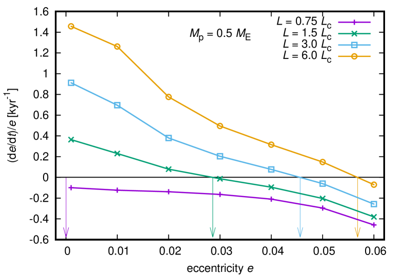
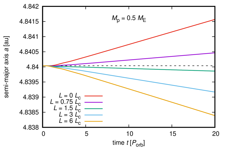
Figure 13: Supplementary figures for $M_{\mathrm{p}}=0.5\,M_{\earth}$. Top: as in Fig. 4, middle: as in Fig. 6, bottom: as in Fig. 7.

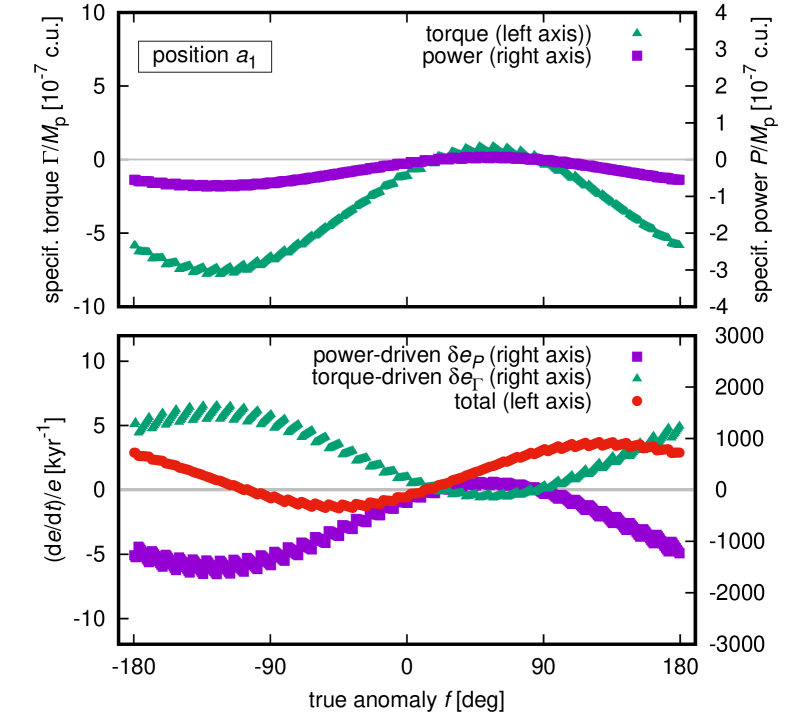
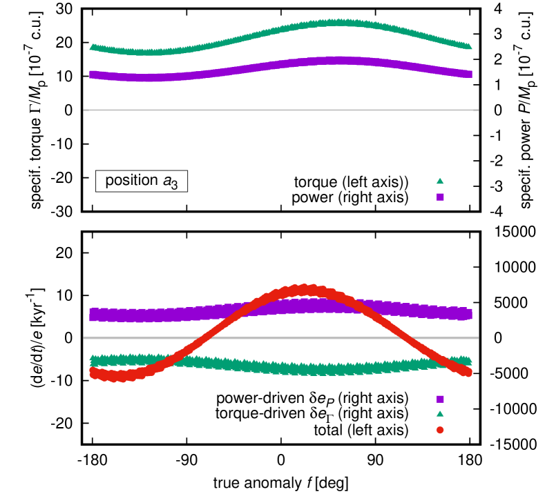
Figure 14: Analysis of the torque, power, and eccentricity evolution rate for $M_{\mathrm{p}}=1\,M_{\earth}$, $L=3\,L_{\mathrm{c}}$, and $e=0.001$ at the initial semi-major axes $a_{1}$ (left) and $a_{3}$ (right). Top: Specific torque $\Gamma/M_{\mathrm{p}}$ (purple squares, primary vertical axis) and power $P/M_{\mathrm{p}}$ (green triangles, secondary vertical axis) as a function of the true anomaly $f$. Bottom: Eccentricity evolution rate $\dot{e}/e$ (red circles, primary vertical axis), and its components driven by the disc power $\delta e_{P}$ (purple squares, secondary vertical axis) and disc torque $\delta e_{\Gamma}$ (green triangles, secondary vertical axis). Data points were recorded over the last 10 orbits of the planet.

Appendix B Eccentricity growth in the shear-dominated regime

We demonstrated in Section 3.6, for the case of circular orbits, that the influence of thermal torques on the semi-major axis evolution at $a_{2}$ and $a_{3}$ is in agreement with previous studies (e.g. Benítez-Llambay et al., 2015), while it can facilitate inward migration in the super-Keplerian region near $a_{1}$. However, the eccentricity evolution rate is quite similar at $a_{1}$, $a_{2}$, and $a_{3}$ (Fig. 5).

To provide more insight into the eccentricity evolution in the shear-dominated regime, we performed two simulations at $a_{1}$ and $a_{3}$ for the parameters $M_{\mathrm{p}}=1\,M_{\earth}$, $e=0.001$, and $L=3\,L_{\mathrm{c}}$. These simulations were performed over 20 orbits and the planets were free to migrate. We measured the disc torque $\Gamma$ and power $P$ with the aim to relate them to the eccentricity evolution rate. To do so, one can utilize (Bitsch & Kley, 2010)

$$\frac{\dot{e}}{e}=\frac{1-e^{2}}{e^{2}}\left(\frac{1}{2}\frac{\dot{a}}{a}-\frac{\Gamma}{L}\right)\coloneqq\delta e_{P}+\delta e_{\Gamma}\,,$$ (16)

where $\dot{a}/a$ comes from Equation (13) and the orbital angular momentum is

$$L=\mu\sqrt{GMa\left(1-e^{2}\right)}\,,$$ (17)

where $M=M_{\star}+M_{\mathrm{p}}$ and $\mu=M_{\star}M_{\mathrm{p}}/M$. In writing Equation (16), we split the expression into a power-driven term $\delta e_{P}$ and a torque-driven term $\delta e_{\Gamma}$.

Fig. 14 shows $\Gamma$, $P$, $\delta e_{\Gamma}$, $\delta e_{P}$, and $\dot{e}/e$ as functions of the true anomaly $f$. We can therefore infer how the instantaneous change of the orbital angular momentum and energy propagates into the change of $e$ during orbital cycles of the planet. First, we notice that $P$ is negative at $a_{1}$ while it is positive at $a_{3}$. This corresponds to the opposite $\dot{a}$ at these two locations (see Equation 13). Second, $\dot{e}$ oscillates during each orbit but the positive values clearly dominate on average and as a result, $e$ grows both at $a_{1}$ and $a_{3}$. However, there is a systematic difference between the profiles of $\dot{e}(f)/e$. For $a_{1}$, $\dot{e}$ is zero when the planet is at the pericentre, then it follows a broad positive peak as the planet moves towards the apocentre, and a small negative peak occurs between $f=-90^{\circ}$ and $0^{\circ}$. For $a_{3}$, the maximum (minimum) of $\dot{e}$ occurs roughly at the pericentre (apocentre).

Appendix C Connection to detailed opacity models

In our disc model, we assumed a constant uniform opacity $\kappa=1\,\mathrm{cm}^{2}\,\mathrm{g}^{-1}$. Whether this value is realistic or not depends mostly on the dust composition and grain sizes in the given disc region. To provide at least one quantitative comparison of our $\kappa$ with a more detailed opacity model, we calculated frequency-dependent dust opacities $\kappa_{\nu,\mathrm{d}}$ using the Optool code (Dominik et al., 2021), while assuming the DIANA standard for the dust grain composition and size-frequency distribution (Woitke et al., 2016). Subsequently, we converted $\kappa_{\nu,\mathrm{d}}$ into the Rosseland mean opacities $\kappa_{\mathrm{R}}$, which are commonly used to describe the transfer of thermal radiation in the gray diffusion approximation. Finally, since $\kappa$ is used in our model to calculate optical depths in the gas, we rescaled $\kappa_{\mathrm{R}}$ by multiplying it with the canonical dust-to-gas ratio of the interstellar medium $f_{\mathrm{d2g}}=0.01$.

Fig. 15 shows the scaled Rosseland opacities as a function of the local disc temperature $T$. At radial positions $a_{1}$, $a_{2}$, and $a_{3}$, which are highlighted with vertical dashed lines, we can see that $\kappa=1\,\mathrm{cm}^{2}\,\mathrm{g}^{-1}$ differs from the Rosseland opacity curve by 6, 9, and 15 per cent, respectively.

Figure 15: Frequency-averaged Rosseland opacity $\kappa_{R}$ as a function of the local disc temperature $T$. To calculate $\kappa_{R}$, we considered the standard DIANA dust grain composition and we also scaled $\kappa_{R}$ by the typical dust-to-gas ratio $f_{\mathrm{d2g}}=0.01$. The vertical dashed lines show the temperature of our unperturbed disc at locations $a_{1}$, $a_{2}$, and $a_{3}$. The opacity curve can be readily compared with the choice of the uniform opacity $\kappa=1\,\mathrm{cm^{2}}\,\mathrm{g}^{-1}$ used in our simulations.

References

- Andama et al. (2022) Andama G., Ndugu N., Anguma S. K., Jurua E., 2022, MNRAS, 512, 5278
- Andrews et al. (2018) Andrews S. M., et al., 2018, ApJ, 869, L41
- Appelgren et al. (2023) Appelgren J., Lambrechts M., van der Marel N., 2023, A&A, 673, A139
- Ataiee & Kley (2021) Ataiee S., Kley W., 2021, A&A, 648, A69
- Ataiee et al. (2014) Ataiee S., Dullemond C. P., Kley W., Regály Z., Meheut H., 2014, A&A, 572, A61
- Baruteau & Masset (2008) Baruteau C., Masset F., 2008, ApJ, 678, 483
- Baruteau & Masset (2013) Baruteau C., Masset F., 2013, in Souchay J., Mathis S., Tokieda T., eds, Lecture Notes in Physics, Berlin Springer Verlag Vol. 861, Lecture Notes in Physics, Berlin Springer Verlag. p. 201 (arXiv:1203.3294), doi:10.1007/978-3-642-32961-6_6
- Benítez-Llambay & Masset (2016) Benítez-Llambay P., Masset F. S., 2016, ApJS, 223, 11
- Benítez-Llambay et al. (2015) Benítez-Llambay P., Masset F., Koenigsberger G., Szulágyi J., 2015, Nature, 520, 63
- Bitsch (2019) Bitsch B., 2019, A&A, 630, A51
- Bitsch & Kley (2010) Bitsch B., Kley W., 2010, A&A, 523, A30
- Bitsch & Kley (2011) Bitsch B., Kley W., 2011, A&A, 536, A77
- Bitsch et al. (2013) Bitsch B., Crida A., Morbidelli A., Kley W., Dobbs-Dixon I., 2013, A&A, 549, A124
- Bitsch et al. (2014) Bitsch B., Morbidelli A., Lega E., Crida A., 2014, A&A, 564, A135
- Bitsch et al. (2019) Bitsch B., Raymond S. N., Izidoro A., 2019, A&A, 624, A109
- Brož et al. (2021) Brož M., Chrenko O., Nesvorný D., Dauphas N., 2021, Nature Astronomy, 5, 898
- Chambers (2021) Chambers J., 2021, ApJ, 914, 102
- Chametla & Chrenko (2022) Chametla R. O., Chrenko O., 2022, MNRAS, 512, 2189
- Chametla & Masset (2021) Chametla R. O., Masset F. S., 2021, MNRAS, 501, 24
- Chametla et al. (2022) Chametla R. O., Masset F. S., Baruteau C., Bitsch B., 2022, MNRAS, 510, 3867
- Chrenko & Lambrechts (2019) Chrenko O., Lambrechts M., 2019, A&A, 626, A109
- Chrenko & Nesvorný (2020) Chrenko O., Nesvorný D., 2020, A&A, 642, A219
- Chrenko et al. (2017) Chrenko O., Brož M., Lambrechts M., 2017, A&A, 606, A114
- Chrenko et al. (2022) Chrenko O., Chametla R. O., Nesvorný D., Flock M., 2022, A&A, 666, A63
- Cieza et al. (2019) Cieza L. A., et al., 2019, MNRAS, 482, 698
- Commerçon et al. (2011) Commerçon B., Teyssier R., Audit E., Hennebelle P., Chabrier G., 2011, A&A, 529, A35
- Cornejo et al. (2023) Cornejo S., Masset F. S., Chametla R. O., Fromenteau S., 2023, MNRAS,
- Dipierro et al. (2018) Dipierro G., et al., 2018, MNRAS, 475, 5296
- Dominik et al. (2021) Dominik C., Min M., Tazaki R., 2021, Astrophysics Source Code Library, p. ascl:2104.010
- Dullemond et al. (2018) Dullemond C. P., et al., 2018, ApJ, 869, L46
- Eklund & Masset (2017) Eklund H., Masset F. S., 2017, MNRAS, 469, 206
- Fendyke & Nelson (2014) Fendyke S. M., Nelson R. P., 2014, MNRAS, 437, 96
- Flock et al. (2016) Flock M., Fromang S., Turner N. J., Benisty M., 2016, ApJ, 827, 144
- Flock et al. (2019) Flock M., Turner N. J., Mulders G. D., Hasegawa Y., Nelson R. P., Bitsch B., 2019, A&A, 630, A147
- Fromenteau & Masset (2019) Fromenteau S., Masset F. S., 2019, MNRAS, 485, 5035
- Goldreich & Tremaine (1979) Goldreich P., Tremaine S., 1979, ApJ, 233, 857
- Guilera et al. (2019) Guilera O. M., Cuello N., Montesinos M., Miller Bertolami M. M., Ronco M. P., Cuadra J., Masset F. S., 2019, MNRAS, 486, 5690
- Guilera et al. (2020) Guilera O. M., Sándor Z., Ronco M. P., Venturini J., Miller Bertolami M. M., 2020, A&A, 642, A140
- Hankla et al. (2020) Hankla A. M., Jiang Y.-F., Armitage P. J., 2020, ApJ, 902, 50
- Hubeny (1990) Hubeny I., 1990, ApJ, 351, 632
- Izidoro et al. (2021) Izidoro A., Bitsch B., Raymond S. N., Johansen A., Morbidelli A., Lambrechts M., Jacobson S. A., 2021, A&A, 650, A152
- Jiang & Ormel (2023) Jiang H., Ormel C. W., 2023, MNRAS, 518, 3877
- Jiménez & Masset (2017) Jiménez M. A., Masset F. S., 2017, MNRAS, 471, 4917
- Klahr & Kley (2006) Klahr H., Kley W., 2006, A&A, 445, 747
- Klahr et al. (2018) Klahr H., Pfeil T., Schreiber A., 2018, Instabilities and Flow Structures in Protoplanetary Disks: Setting the Stage for Planetesimal Formation. p. 138, doi:10.1007/978-3-319-55333-7_138
- Kley et al. (2009) Kley W., Bitsch B., Klahr H., 2009, A&A, 506, 971
- Lambrechts & Johansen (2012) Lambrechts M., Johansen A., 2012, A&A, 544, A32
- Lambrechts & Johansen (2014) Lambrechts M., Johansen A., 2014, A&A, 572, A107
- Lambrechts et al. (2014) Lambrechts M., Johansen A., Morbidelli A., 2014, A&A, 572, A35
- Lau et al. (2022) Lau T. C. H., Drążkowska J., Stammler S. M., Birnstiel T., Dullemond C. P., 2022, A&A, 668, A170
- Lega et al. (2014) Lega E., Crida A., Bitsch B., Morbidelli A., 2014, MNRAS, 440, 683
- Lesur et al. (2022) Lesur G., et al., 2022, arXiv e-prints, p. arXiv:2203.09821
- Liu & Ormel (2018) Liu B., Ormel C. W., 2018, A&A, 615, A138
- Lovelace et al. (1999) Lovelace R. V. E., Li H., Colgate S. A., Nelson A. F., 1999, ApJ, 513, 805
- Masset (2001) Masset F. S., 2001, ApJ, 558, 453
- Masset (2017) Masset F. S., 2017, MNRAS, 472, 4204
- Masset & Velasco Romero (2017) Masset F. S., Velasco Romero D. A., 2017, MNRAS, 465, 3175
- Masset et al. (2006) Masset F. S., Morbidelli A., Crida A., Ferreira J., 2006, ApJ, 642, 478
- Mihalas & Weibel Mihalas (1984) Mihalas D., Weibel Mihalas B., 1984, Foundations of radiation hydrodynamics. Oxford University Press, New York
- Morbidelli (2020) Morbidelli A., 2020, A&A, 638, A1
- Morbidelli & Nesvorný (2012) Morbidelli A., Nesvorný D., 2012, A&A, 546, A18
- Mulders et al. (2018) Mulders G. D., Pascucci I., Apai D., Ciesla F. J., 2018, AJ, 156, 24
- Nakagawa et al. (1986) Nakagawa Y., Sekiya M., Hayashi C., 1986, Icarus, 67, 375
- Nelson et al. (2013) Nelson R. P., Gressel O., Umurhan O. M., 2013, MNRAS, 435, 2610
- Ormel & Klahr (2010) Ormel C. W., Klahr H. H., 2010, A&A, 520, A43
- Paardekooper & Mellema (2006) Paardekooper S.-J., Mellema G., 2006, A&A, 459, L17
- Paardekooper & Mellema (2008) Paardekooper S.-J., Mellema G., 2008, A&A, 478, 245
- Paardekooper et al. (2011) Paardekooper S.-J., Baruteau C., Kley W., 2011, MNRAS, 410, 293
- Pfeil & Klahr (2019) Pfeil T., Klahr H., 2019, ApJ, 871, 150
- Pierens (2023) Pierens A., 2023, MNRAS, 520, 3286
- Pinilla et al. (2012) Pinilla P., Birnstiel T., Ricci L., Dullemond C. P., Uribe A. L., Testi L., Natta A., 2012, A&A, 538, A114
- Shakura & Sunyaev (1973) Shakura N. I., Sunyaev R. A., 1973, A&A, 500, 33
- Stone & Norman (1992) Stone J. M., Norman M. L., 1992, ApJS, 80, 753
- Tanaka & Ward (2004) Tanaka H., Ward W. R., 2004, ApJ, 602, 388
- Tanaka et al. (2002) Tanaka H., Takeuchi T., Ward W. R., 2002, ApJ, 565, 1257
- Teague et al. (2018) Teague R., Bae J., Birnstiel T., Bergin E. A., 2018, ApJ, 868, 113
- Turner et al. (2014) Turner N. J., Fromang S., Gammie C., Klahr H., Lesur G., Wardle M., Bai X. N., 2014, in Beuther H., Klessen R. S., Dullemond C. P., Henning T., eds, Protostars and Planets VI. pp 411–432 (arXiv:1401.7306), doi:10.2458/azu_uapress_9780816531240-ch018
- Ueda et al. (2017) Ueda T., Okuzumi S., Flock M., 2017, ApJ, 843, 49
- Velasco Romero et al. (2022) Velasco Romero D. A., Masset F. S., Teyssier R., 2022, MNRAS, 509, 5622
- Venturini et al. (2020) Venturini J., Guilera O. M., Ronco M. P., Mordasini C., 2020, A&A, 644, A174
- Ward (1991) Ward W. R., 1991, in Lunar and Planetary Science Conference.
- Weber et al. (2019) Weber P., Pérez S., Benítez-Llambay P., Gressel O., Casassus S., Krapp L., 2019, ApJ, 884, 178
- Woitke et al. (2016) Woitke P., et al., 2016, A&A, 586, A103
- de Val-Borro et al. (2006) de Val-Borro M., et al., 2006, MNRAS, 370, 529