Geometrically Parametrised Reduced Order Models for Studying the Hysteresis of the Coanda Effect in Finite-elements-based Incompressible Fluid Dynamics

Abstract

This article presents a general reduced order model (ROM) framework for addressing fluid dynamics problems involving time-dependent geometric parametrisations. The framework integrates Proper Orthogonal Decomposition (POD) and Empirical Cubature Method (ECM) hyper-reduction techniques to effectively approximate incompressible computational fluid dynamics simulations. To demonstrate the applicability of this framework, we investigate the behavior of a planar contraction-expansion channel geometry exhibiting bifurcating solutions known as the Coanda effect. By introducing time-dependent deformations to the channel geometry, we observe hysteresis phenomena in the solution.

The paper provides a detailed formulation of the framework, including the stabilised finite elements full order model (FOM) and ROM, with a particular focus on the considerations related to geometric parametrisation. Subsequently, we present the results obtained from the simulations, analysing the solution behavior in a phase-space for the fluid velocity at a probe point, considered as the Quantity of Interest (QoI). Through qualitative and quantitative evaluations of the ROMs and hyper-reduced order models (HROMs), we demonstrate their ability to accurately reproduce the complete solution field and the QoI.

While HROMs offer significant computational speedup, enabling efficient simulations, they do exhibit some errors, particularly for testing trajectories. However, their value lies in applications where the detection of the Coanda effect holds paramount importance, even if the selected bifurcation branch is incorrect. Alternatively, for more precise results, HROMs with lower speedups can be employed.

1 Introduction

This study focuses on projection-based reduced order models for fluid dynamics problems with time-dependent geometric parametrisations. We solve the Navier-Stokes equations on a parametrised domain denoted as $\Omega(\boldsymbol{\mu})\subset\mathbb{R}^{d}$ , with a time span $[0,T]$. Later on, in section 2.1, the specific form of the equations is shown. The geometric parametrisation is defined via a mapping $\varphi(\boldsymbol{\mu}):\Omega_{0}\times\mathcal{P}\rightarrow\Omega$, such that, given a parameter $\boldsymbol{\mu}\in\mathcal{P}\subset\mathbb{R}^{p}$, each point in the original configuration is mapped onto a corresponding point in the deformed one as in Fig. 1.

Figure 1: Transformation of a domain $\Omega_{0}$ into $\Omega$ via a mapping $\varphi$

The particular case we are focusing on in this study involves a planar contraction-expansion channel. This simple geometry has been widely used in both experimental and numerical investigations [31, 29, 7]. This case was chosen due to its tendency to exhibit complex dynamics, even at relatively low Reynolds numbers. A noteworthy characteristic of the model is that it leads to the emergence of the so-called Coanda effect [47], which is characterised by an asymmetric jet adhering to an adjacent wall.

The inherent nonlinearity of the Navier-Stokes equations can give rise to a bifurcation phenomenon in the solution. Within a certain range of values for the driving parameter, typically the Reynolds number in most computational fluid dynamics (CFD) problems, a unique solution exists. However, once a critical point is surpassed, it is possible for multiple solutions to coexist for the same Reynolds number value [2].

Figure 2: For $Re<{Re}_{\text{\tiny SB}}\$ there exists a unique solution. For $Re\geq Re_{\text{\tiny SB}}$ three solutions coexist

In this investigation, the variation in geometry acts as the sole driving factor for the Reynolds number. The viscosity and density of the fluid remain constant throughout the study, and once the fluid is initialised, the boundary conditions remain unchanged. In this setting, as the width of the channel narrows, the Reynolds number increases.

The fluid development in a contraction-expansion channel can be described as follows:

• For sufficiently small values of the Reynolds number, there exists a single perfectly symmetric solution, exhibiting symmetry in both the horizontal and vertical directions.

• As the Reynolds number increases, the horizontal symmetry of the solution is lost, but the solution remains symmetric about the vertical axis. This results in the formation of a symmetric jet.

• At a critical Reynolds number value, denoted as ${Re}_{\text{\tiny SB}}$ (see Fig. 2), the symmetry of the jet is disrupted due to the Coanda Effect. In this scenario, the jet attaches itself to either the upper or lower wall. While the symmetric jet solution is still mathematically possible, it becomes unstable. Numerical simulations or experiments typically yield one of the non-symmetric solutions unless advanced techniques are employed to extract the unstable solution, for instance, when constructing the complete bifurcation diagram [33, 32].

• With further increases in the Reynolds number, the presence of eddies becomes prominent. At a specific critical Reynolds number, denoted as ${Re}_{\text{\tiny H}}$, a Hopf bifurcation occurs, resulting in the emergence of an oscillating solution. However, the discussion of the Hopf bifurcation lies beyond the scope of this work. Interested readers are referred e.g. to [36, 42] for further exploration of Hopf bifurcations.

The contraction-expansion channel has previously been utilised in research on mitral valve regurgitation disease, as demonstrated in studies such as [34]. This disease is characterised by the improper closure of the mitral valve, as depicted in Fig 3. As a result of this faulty closure, blood is able to flow through a narrow opening, giving rise to the wall-hugging behavior mentioned earlier.

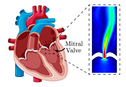
Figure 3: Mitral valve of the human heart and the contraction-expansion channel model used in this investigation. Contraction-expansion channel models can help in the study of mitral valve regurgitation disease

Previous numerical studies on the contraction-expansion channel have utilised an affine mapping $\varphi(\boldsymbol{\mu})$, in conjunction with the spectral element method (SEM)[18]. The affine nature of the geometric mapping in that study facilitated a complete online-offline decoupling of the reduced-order models, eliminating the need for additional interpolation and achieving significant speedup factors for the reduced-order models.

In a subsequent study [17], a nonlinear geometric mapping was introduced to account for walls with varying curvature. To effectively evaluate the reduced-order models in this scenario, the discrete empirical interpolation (DEIM) method was employed [6, 37].

More recently, the fluid-structure interaction problem has been investigated by incorporating (hyper)elastic walls [22]. In that case, the deformation of the walls was computed from their interaction with the flow, rather than being imposed. For the present work, we will adhere to the approach of explicitly imposing the walls deformation.

Furthermore, in [32] a non-intrusive neural network framework, known as POD-NN, was employed for efficiently approximating the bifurcating phenomena in a contraction-expansion channel, as well as in other geometries.

In the aforementioned studies, the main objective was to construct the bifurcation diagram. To achieve this goal, steady-state solutions were computed for each parameter variation. This means that even when the geometry was parametrised, the geometric parametrisation remained unchanged over time. The focus was on capturing the steady-state behavior of the system and analyzing the bifurcation phenomena, rather than considering time-dependent variations in the geometric parametrisation.

Time dependent geometry variations for studying wall-hugging phenomena in flow jets have been investigated for example in [1]. In that work, both numerical and experimental setups were applied to study the Coanda effect on jets interacting with inclined planes. The parameter to vary was the angle of the plate at the exit of the jet. It was observed that as the inclination angle of the planes was varied, the jet eventually attached, detached, or re-attached to either one of the walls, depending on whether the inclination angle was being increased or decreased. Thus, resulting on a hysteresis loop. This hysteresis phenomena in fluid problems exhibiting bifurcations had already been reported in classical works [30, 23], and more recently in [35, 41, 41]

Our main contributions in this study expand on the existing literature by considering a contraction-expansion channel geometry that undergoes time-dependent deformations. By incorporating this dynamically morphed geometry, we are able to observe hysteresis phenomena in the solution, which has been previously documented in works such as [35].

Moreover, the framework presented in this work offers broad applicability to a range of geometrically parametrised ROMs. This versatility allows for the framework to be employed in various scenarios. Unlike previous approaches that rely on assumptions about the nature of the mapping $\varphi(\boldsymbol{\mu})$ to achieve efficient offline-online decoupling, as seen in works like [24, 27, 37, 18], we achieve efficient offline-online decoupling through the use of the empirical cubature method (ECM) [15, 14]. ECM is a mesh-sampling and weighting hyper-reduction technique that has been successfully employed in several studies to attain high computational efficiency.

This paper is structured as follows. In Chapter 2, we present the formulation of the general framework for the fluid problem, including the formulations for the reduced and hyper-reduced order models. Section 3 provides a detailed description of the finite element model utilised in this study, along with the two different geometric mappings employed. One mapping involves an affine transformation with straight walls, while the other employs a nonlinear mapping with curved walls. The obtained results are presented in Section 4. Finally, in Section 5, we discuss the conclusions drawn from this study and provide insights into future research directions.

2 Formulation

In order to maintain this paper as self-contained as possible, this section presents a concise overview of the stabilised finite element discretisation of the governing equations employed in this study. We then introduce the Galerkin Proper Orthogonal Decomposition (POD-Galerkin) and the Empirical Cubature Method (ECM) hyper-reduction techniques, highlighting the specific considerations related to the geometrically parametrised problem under investigation. We conclude the chapter by providing a summary of the simulation workflow for all the models employed in this study.

2.1 Governing Equations

As mentioned earlier in the introduction, we now proceed to explicitly state the fluids problem. The governing equations consirered are the standard Differential-Algebraic incompressible Navier-Stokes equations in an Arbitrary Lagrangian Eulerian (ALE) frame of reference

$$\left\{\begin{array}[]{ll}\frac{\partial\boldsymbol{u}}{\partial t}+(\boldsymbol{c}\cdot\nabla)\boldsymbol{u}-\boldsymbol{b}-\nabla\cdot\boldsymbol{\sigma}=\boldsymbol{0}&\mathrm{in\ \ }\Omega(\boldsymbol{\mu})\times(0,T]\ ,\\ \nabla\cdot\boldsymbol{u}=0&\mathrm{in\ \ }\Omega(\boldsymbol{\mu})\times(0,T]\ ,\end{array}\right.$$ (1)

where $\boldsymbol{u}$ is the velocity, $\boldsymbol{b}$ are the body forces, $\boldsymbol{\sigma}=-p\boldsymbol{I}+2\nu\nabla^{s}\boldsymbol{u}$ is the Cauchy stress tensor, $p$ is the pressure, $\nu$ is the kinematic viscosity, $\boldsymbol{c}=\boldsymbol{u}-\hat{\boldsymbol{u}}$ is the convective velocity, and $\hat{\boldsymbol{u}}$ is the so-called mesh velocity which results from the deformation of the domain and is a datum to the fluids problem. The governing equations, taking into account the provided expressions, can be written as follows:

$$\left\{\begin{array}[]{ll}\frac{\partial\boldsymbol{u}}{\partial t}+\nabla\cdot(\boldsymbol{c}\otimes\boldsymbol{u})-\boldsymbol{b}+\nabla p-\nabla\cdot(2\nu\nabla^{s}\boldsymbol{u})=\boldsymbol{0}&\mathrm{in\ \ }\Omega(\boldsymbol{\mu})\times(0,T]\ ,\\ \nabla\cdot\boldsymbol{u}=0&\mathrm{in\ \ }\Omega(\boldsymbol{\mu})\times(0,T]\ .\end{array}\right.$$ (2)

The initial conditions $g_{0}$, and Dirichlet and Neumann boundary conditions $g_{D}$ and $g_{N}$ are case-specific and are specified by the corresponding functions, as:

$$\begin{array}[]{ll}(\boldsymbol{u},p)=g_{0}(\boldsymbol{u},p,\boldsymbol{x})&\mathrm{in\ \ }\Omega(\boldsymbol{\mu})\times\{0\}\ ,\\ \left(2\nu\nabla^{s}\boldsymbol{u}-p\boldsymbol{I}\right)\boldsymbol{n}=g_{N}(\boldsymbol{u},p,\boldsymbol{x})&\mathrm{on\ \ }\partial\Omega_{N}(\boldsymbol{\mu})\times(0,T]\ ,\\ (\boldsymbol{u},p)=g_{D}(\boldsymbol{u},p,\boldsymbol{x})&\mathrm{on\ \ }\partial\Omega_{D}(\boldsymbol{\mu})\times(0,T]\ ,\end{array}$$ (3)

with $\partial\Omega_{N}(\boldsymbol{\mu})\cup\partial\Omega_{D}(\boldsymbol{\mu})=\partial\Omega(\boldsymbol{\mu})$ and $\partial\Omega(\boldsymbol{\mu})_{N}\cap\partial\Omega(\boldsymbol{\mu})_{D}=\emptyset$.

2.2 Full Order Model FOM

Let us introduce the functional spaces to pose the weak formulation for the space discretisation as

$$\mathcal{V}:=\{\boldsymbol{v}\in H^{1}(\Omega)\mid\boldsymbol{v}=\boldsymbol{0}\text{ on }\partial\Omega_{D}\}\ ,\hskip 22.76219pt\mathcal{Q}:=L^{2}(\Omega)\ .$$ (4)

In what follows, we will use the standard $L^{2}(\Omega)$ inner product notation $(\cdot,\cdot)_{\Omega}$ for brevity. The weak form of the governing equations in Eq. 2 is then given by:

$$\left\{\begin{array}[]{ll}\left(\frac{\partial\boldsymbol{u}}{\partial t},\boldsymbol{v}\right)_{\Omega}-\left(\boldsymbol{c}\otimes\boldsymbol{u},\nabla\boldsymbol{v}\right)_{\Omega}+2\nu\left(\nabla^{s}\boldsymbol{u},\nabla^{s}\boldsymbol{v}\right)_{\Omega}-\left(p,\nabla\cdot\boldsymbol{v}\right)_{\Omega}-\left(\boldsymbol{b},\boldsymbol{v}\right)_{\Omega}=\boldsymbol{0}&\forall\boldsymbol{\boldsymbol{v}}\in\mathcal{V}\ ,\\ \left(q,\nabla\cdot\boldsymbol{u}\right)_{\Omega}=0&\forall q\in\mathcal{Q}\ .\end{array}\right.$$ (5)

We define the finite element spaces $\mathcal{V}^{h}\subset\mathcal{V}$ and $\mathcal{Q}^{h}\subset\mathcal{Q}$. These spaces are spanned respectively by a set of basis functions $\{\boldsymbol{\psi}_{i}\}_{i=1}^{N_{v}}$ and $\{\hat{\psi}_{j}\}_{j=1}^{N_{p}}$, being $\text{dim}\mathcal{V}^{h}=N_{v}$, and $\text{dim}\mathcal{Q}^{h}=N_{p}$. The finite elements weak form of the governing equations can be expressed as follows:

$$\left\{\begin{array}[]{ll}\left(\frac{\partial\boldsymbol{u}^{h}}{\partial t},\boldsymbol{v}^{h}\right)_{\Omega}-\left(\boldsymbol{c}^{h}\otimes\boldsymbol{u}^{h},\nabla\boldsymbol{v}^{h}\right)_{\Omega}+2\nu\left(\nabla^{s}\boldsymbol{u}^{h},\nabla^{s}\boldsymbol{v}^{h}\right)_{\Omega}-\left(p^{h},\nabla\cdot\boldsymbol{v}^{h}\right)_{\Omega}-\left(\boldsymbol{b},\boldsymbol{v}^{h}\right)_{\Omega}=\boldsymbol{0}&\forall\boldsymbol{\boldsymbol{v}}^{h}\in\mathcal{V}^{h}\ ,\\ \left(q^{h},\nabla\cdot\boldsymbol{u}^{h}\right)_{\Omega}=0&\forall q^{h}\in\mathcal{Q}^{h}\ ,\end{array}\right.$$ (6)

where $\boldsymbol{c}^{h}=\boldsymbol{u}^{h}-\hat{\boldsymbol{u}}^{h}$ is the finite elements convective velocity.

To ensure the well-posedness of the problem, the selected spaces for the approximation of pressure and velocity should be compatible and satisfy the Ladyzhenskaya–Babuška–Brezzi (LBB) condition [11]. The LBB condition can be stated as follows:

$$\inf_{q^{h}\in\mathcal{Q}^{h}}\sup_{\boldsymbol{v}^{h}\in\mathcal{V}^{h}}\frac{\left(q^{h},\nabla\cdot\boldsymbol{v}^{h}\right)}{\left\lVert q^{h}\right\rVert_{\mathcal{Q}^{h}}\left\lVert\boldsymbol{v}^{h}\right\rVert_{\mathcal{V}^{h}}}\geq\alpha>0\hskip 14.22636pt\iff\hskip 14.22636pt\exists\ (\boldsymbol{u}^{h}\in\mathcal{V}^{h},q\in\mathcal{Q}^{h})\ .$$ (7)

LBB compatible spaces necessarily comply with

$$\text{dim}\mathcal{Q}^{h}\leq\text{dim}\mathcal{V}^{h}\Leftarrow\hskip 14.22636pt\exists\ (\boldsymbol{u}^{h}\in\mathcal{V}^{h},q\in\mathcal{Q}^{h})\ ,$$ (8)

however, in this work, we aim to use the same order of interpolation for the finite element approximation of both variables. To overcome the limitation imposed by the LBB condition, we employ the Variational Multiscale (VMS) stabilisation technique [9, 10, 43].

2.2.1 Variational Multiscale VMS Stabilisation

The VMS approach introduces subgrid spaces $\mathcal{V}^{\prime}$ and $\mathcal{Q}^{\prime}$, defined as:

$$\mathcal{V}=\mathcal{V}^{h}\oplus\mathcal{V}^{\prime}\ ,\hskip 19.91692pt\mathcal{Q}=\mathcal{Q}^{h}\oplus\mathcal{Q}^{\prime}\ ,$$ (9)

where $\oplus$ denotes the direct sum. The complementary velocity and pressure functions $(\boldsymbol{u}^{\prime},p^{\prime})$ are such that

$$\begin{split}\boldsymbol{u}=\boldsymbol{u}^{h}+\boldsymbol{u}^{\prime}\hskip 14.22636pt,\hskip 14.22636pt\boldsymbol{u}^{h}\in\mathcal{V}^{h}\ \ ,\ \boldsymbol{u}^{\prime}\in\mathcal{V}^{\prime}\ ,\\ p=p^{h}+p^{\prime}\hskip 14.22636pt,\hskip 14.22636ptp^{h}\in\mathcal{Q}^{h}\ \ ,\ p^{\prime}\in\mathcal{Q}^{\prime}\ ,\\ \boldsymbol{u}^{\prime}=\boldsymbol{0}\text{ on }\partial\Omega_{D}(\boldsymbol{\mu})\ ,\hskip 14.22636pt\boldsymbol{u}^{h}=g_{D}^{h}\text{ on }\partial\Omega_{D}(\boldsymbol{\mu})\ .\end{split}$$ (10)

In VMS, the complementary functions are modelled as

$$\boldsymbol{u}^{\prime}=-\tau_{M}r_{M}(\boldsymbol{u}^{h},p^{h})\ ,\hskip 19.91692ptp^{\prime}=-\tau_{C}r_{C}(\boldsymbol{u}^{h})\ ,$$ (11)

where the terms $\tau_{M}$ and $\tau_{C}$ represent respectively the momentum and mass conservation residuals defined as

$$\begin{array}[]{l}r_{M}(\boldsymbol{u}^{h},p^{h})=\frac{\partial\boldsymbol{u}^{h}}{\partial t}+\nabla\cdot(\boldsymbol{c}^{h}\otimes\boldsymbol{u}^{h})-\nabla\cdot(2\nu\nabla^{s}\boldsymbol{u}^{h})+\nabla p^{h}-\boldsymbol{b}\ ,\\ r_{C}(\boldsymbol{u}^{h})=\nabla\cdot\boldsymbol{u}^{h}\ .\end{array}$$ (12)

The modelling of the complementary functions with respect to the residuals ensures the consistency of the method, moreover the selection of $\tau_{M}$ and $\tau_{C}$ depends on the specific type of VMS to apply. For example, considering $\tau_{M},\tau_{C}=0$ leads to the Galerkin method. In the case of the quasi-static variational multiscale (QSVMS), which we employ in this study, the time evolution of the complementary functions is neglected [9].

To proceed with an algebraic formulation, we consider a spatial tessellation of the domain $\bar{\Omega}$ into $N_{el}$ finite elements, such that $\bigcup_{e=1}^{N_{el}}\Omega_{e}=\bar{\Omega}$; moreover we specify standard finite elements shape functions with compact support and equal degree of interpolation. The velocity and pressure algebraic vectors are obtained by collecting the nodal solutions for both variables as $\mathbf{u}=\left(u_{1},u_{2},\dots,u_{dN_{n}}\right)^{T}$ and $\mathbf{p}=\left(p_{1},p_{2},\dots,p_{N_{n}}\right)^{T}$, where $N_{n}$ is the number of nodes, and $d$ is the number of spatial dimensions. The QSVMS semi-discrete system can then be expressed as follows:

$$\left\{\begin{array}[]{lll}\boldsymbol{M}\frac{d\mathbf{u}}{dt}+\boldsymbol{A}\mathbf{u}+\boldsymbol{C}(\mathbf{c})\mathbf{u}+\boldsymbol{D}(\mathbf{u},\mathbf{p})+\boldsymbol{B}^{T}\mathbf{p}=\boldsymbol{F}\ ,\\ \boldsymbol{B}\mathbf{u}=\boldsymbol{E}(\mathbf{u},\mathbf{p})\ ,\end{array}\right.$$ (13)

where the standard Galerkin finite element terms are given by

$$\begin{array}[]{llllll}\boldsymbol{M}&=\mathop{\vphantom{\sum}\mathchoice{\vbox{\hbox{\leavevmode\resizebox{9.20009pt}{}{$\mathrm{A}$}}}}{\vbox{\hbox{\leavevmode\resizebox{10.00012pt}{}{$\mathrm{A}$}}}}{\vbox{\hbox{\leavevmode\resizebox{7.00009pt}{}{$\mathrm{A}$}}}}{\vbox{\hbox{\leavevmode\resizebox{5.00006pt}{}{$\mathrm{A}$}}}}}\slimits@^{e}\boldsymbol{M}^{e}&&M_{ij}^{e}&=\left(\boldsymbol{\psi}_{j},\boldsymbol{\psi}_{i}\right)_{\Omega^{e}}&\textit{the mass matrix}\ ,\\ \boldsymbol{A}&=\mathop{\vphantom{\sum}\mathchoice{\vbox{\hbox{\leavevmode\resizebox{9.20009pt}{}{$\mathrm{A}$}}}}{\vbox{\hbox{\leavevmode\resizebox{10.00012pt}{}{$\mathrm{A}$}}}}{\vbox{\hbox{\leavevmode\resizebox{7.00009pt}{}{$\mathrm{A}$}}}}{\vbox{\hbox{\leavevmode\resizebox{5.00006pt}{}{$\mathrm{A}$}}}}}\slimits@^{e}\boldsymbol{A}^{e}&&A_{ij}^{e}&=\left(\nabla^{s}\boldsymbol{\psi}_{j},\nabla^{s}\boldsymbol{\psi}_{i}\right)_{{\Omega}^{e}}&\textit{the diffusion matrix}\ ,\\ \boldsymbol{C}(\mathbf{c})&=\mathop{\vphantom{\sum}\mathchoice{\vbox{\hbox{\leavevmode\resizebox{9.20009pt}{}{$\mathrm{A}$}}}}{\vbox{\hbox{\leavevmode\resizebox{10.00012pt}{}{$\mathrm{A}$}}}}{\vbox{\hbox{\leavevmode\resizebox{7.00009pt}{}{$\mathrm{A}$}}}}{\vbox{\hbox{\leavevmode\resizebox{5.00006pt}{}{$\mathrm{A}$}}}}}\slimits@^{e}\boldsymbol{C}^{e}&&C_{ij}^{e}&=-\left(\boldsymbol{\psi}_{j},\boldsymbol{c}^{h}\cdot\nabla\boldsymbol{\psi}_{i}\right)_{\Omega^{e}}&\textit{the convection matrix}\ ,\\ \boldsymbol{B}&=\mathop{\vphantom{\sum}\mathchoice{\vbox{\hbox{\leavevmode\resizebox{9.20009pt}{}{$\mathrm{A}$}}}}{\vbox{\hbox{\leavevmode\resizebox{10.00012pt}{}{$\mathrm{A}$}}}}{\vbox{\hbox{\leavevmode\resizebox{7.00009pt}{}{$\mathrm{A}$}}}}{\vbox{\hbox{\leavevmode\resizebox{5.00006pt}{}{$\mathrm{A}$}}}}}\slimits@^{e}\boldsymbol{B}^{e}&&B_{ij}^{e}&=-\left(\hat{\psi}_{j},\nabla\cdot\boldsymbol{\psi}_{i}\right)_{\Omega^{e}}&\textit{the pressure/divergence matrix}\ ,\\ \boldsymbol{F}&=\mathop{\vphantom{\sum}\mathchoice{\vbox{\hbox{\leavevmode\resizebox{9.20009pt}{}{$\mathrm{A}$}}}}{\vbox{\hbox{\leavevmode\resizebox{10.00012pt}{}{$\mathrm{A}$}}}}{\vbox{\hbox{\leavevmode\resizebox{7.00009pt}{}{$\mathrm{A}$}}}}{\vbox{\hbox{\leavevmode\resizebox{5.00006pt}{}{$\mathrm{A}$}}}}}\slimits@^{e}\boldsymbol{F}^{e}&&F_{i}^{e}&=\left(b,\boldsymbol{\psi}_{i}\right)_{\Omega^{e}}&\textit{the forcing term}\ ,\end{array}$$ (14)

where $\mathop{\vphantom{\sum}\mathchoice{\vbox{\hbox{\leavevmode\resizebox{9.20009pt}{}{$\mathrm{A}$}}}}{\vbox{\hbox{\leavevmode\resizebox{10.00012pt}{}{$\mathrm{A}$}}}}{\vbox{\hbox{\leavevmode\resizebox{7.00009pt}{}{$\mathrm{A}$}}}}{\vbox{\hbox{\leavevmode\resizebox{5.00006pt}{}{$\mathrm{A}$}}}}}\slimits@^{e}$ is the finite elements assembly operator, $1\leq i,j\leq n_{en}$, and $n_{en}$ is the number of nodes per element. The remaining terms are related to the VMS stabilisation and are defined as follows:

$$\begin{array}[]{llllll}\boldsymbol{D}(\mathbf{u},\mathbf{p})=&\mathop{\vphantom{\sum}\mathchoice{\vbox{\hbox{\leavevmode\resizebox{9.20009pt}{}{$\mathrm{A}$}}}}{\vbox{\hbox{\leavevmode\resizebox{10.00012pt}{}{$\mathrm{A}$}}}}{\vbox{\hbox{\leavevmode\resizebox{7.00009pt}{}{$\mathrm{A}$}}}}{\vbox{\hbox{\leavevmode\resizebox{5.00006pt}{}{$\mathrm{A}$}}}}}\slimits@^{e}\boldsymbol{D}^{e}&&&D_{i}=&\left(\nabla(\boldsymbol{\psi}_{i})\boldsymbol{u}^{h},\tau_{M}r_{M}(\boldsymbol{u}^{h},p^{h})\right)_{\Omega^{e}}\\ &&&&&+\left((\nabla\boldsymbol{\psi}_{i})^{T}\boldsymbol{u}^{h},\tau_{M}r_{M}(\boldsymbol{u}^{h},p^{h})\right)_{\Omega^{e}}\\ &&&&&-\left(\boldsymbol{\psi}_{i},\tau_{M}r_{M}(\boldsymbol{u}^{h},p^{h})\otimes\tau_{M}r_{M}(\boldsymbol{u}^{h},p^{h})\right)_{\Omega^{e}}\\ &&&&&+\left(\tau_{C}r_{C}(\boldsymbol{u}^{h}),\nabla\cdot\boldsymbol{\psi}_{i}\right)_{\Omega^{e}}\ ,\\ \boldsymbol{E}(\mathbf{u},\mathbf{p})=&\mathop{\vphantom{\sum}\mathchoice{\vbox{\hbox{\leavevmode\resizebox{9.20009pt}{}{$\mathrm{A}$}}}}{\vbox{\hbox{\leavevmode\resizebox{10.00012pt}{}{$\mathrm{A}$}}}}{\vbox{\hbox{\leavevmode\resizebox{7.00009pt}{}{$\mathrm{A}$}}}}{\vbox{\hbox{\leavevmode\resizebox{5.00006pt}{}{$\mathrm{A}$}}}}}\slimits@^{e}\boldsymbol{E}^{e}&&&E_{i}=&\left(\nabla\hat{\psi}_{i},\tau_{M}r_{M}(\boldsymbol{u}^{h},p^{h})\right)_{\Omega^{e}}\ .\end{array}$$ (15)

2.2.2 Time Discretisation

We employ a generalised-$\alpha$ time integration scheme [8]. In these schemes, a set of parameters $\gamma,\beta,\alpha_{m},\alpha_{f}$ are defined and used to obtain a linear combination of the terms of the system in Eq. 13 with respect to current and past time steps. Specifically, the Bossak scheme, which is second-order accurate and unconditionally stable, is used in this work. The application of the time integration scheme leads to the fully discrete system:

$$\textbf{K}_{\text{eff}}(\textbf{d}_{n+\ell})\textbf{d}_{n+1}=\textbf{F}_{\text{eff}}\ ,$$ (16)

where $\textbf{K}_{\text{eff}}(\textbf{d}_{n+\ell})\in\mathbb{R}^{\mathcal{N}\times\mathcal{N}}$ is the fully discrete system matrix, $\mathcal{N}$ is the total number of degrees of freedom, $\textbf{d}_{n+1}\in\mathbb{R}^{\mathcal{N}}$ is the finite elements solution vector at time step $n+1$, that is

$$\textbf{d}_{n+1}=\begin{bmatrix}\mathbf{u}_{n+1}\\ \mathbf{p}_{n+1}\end{bmatrix}\ .$$ (17)

The dependence of the matrix $\textbf{K}_{\text{eff}}(\textbf{d}_{n+\ell})$ on the solution is due to the nonlinearity in the convective term, the subscript $n+\ell$ depends on the type of linearisation used. We now spend a word on the linearisation technique employed.

2.2.3 Linearisation of the Discrete System

Given a solution at a time step $n$, the solution corresponding to time step $n+1$ is written in incremental form as

$$\textbf{d}_{n+1}=\textbf{d}_{n}+{\boldsymbol{\Delta}\textbf{d}}_{n+1}\ ,$$ (18)

where $\boldsymbol{\Delta d}\in\mathbb{R}^{\mathcal{N}}$ is a solution increment. We define the residual $\textbf{R}:\mathbb{R}^{\mathcal{N}}\times\mathcal{P}\rightarrow\mathbb{R}^{\mathcal{N}}$ (highlighting the dependence of all terms of the residual on the geometric parameter $\boldsymbol{\mu}\in\mathcal{P}$), as

$$\textbf{R}(\textbf{d}_{n+1};\boldsymbol{\mu}):=\textbf{F}_{\text{eff}}-\textbf{K}_{\text{eff}}(\textbf{d}_{n+\ell})\textbf{d}_{n+1}\ ,$$ (19)

together with a fixed-point iteration method of the form

$$-\textbf{J}(\textbf{d}_{n+1}^{k})\delta\textbf{d} =\textbf{R}(\textbf{d}_{n+1}^{k})\ ,$$ (20a)

$${\boldsymbol{\Delta}\textbf{d}}_{n+1}^{k+1} ={\boldsymbol{\Delta}\textbf{d}}^{k+1}_{n+1}+\delta\textbf{d}\ ,$$ (20b)

where the Jacobian matrix $\textbf{J}=\partial\textbf{R}/\partial\textbf{d}$, and $k$ is the current iterate index. We use a Picard method [11], which amounts to choosing $\ell=0$ for the matrix $\textbf{K}_{\text{eff}}(\textbf{d}_{n+\ell})$ in Eq. 19. A Newton-Raphson method would amount to choosing the subindex $\ell=1$, and therefore taking the tangent in the current iterate.

2.2.4 Quantity of Interest QoI

It is not uncommon that, rather than the complete solution field d, a quantity of interest is computed through a given operator $\Gamma$ on the solution field as:

$$\textbf{z}=\Gamma(\textbf{d}),\hskip 14.22636pt\textbf{z}\in\mathbb{R}^{\alpha}\subseteq\mathbb{R}^{\mathcal{N}}\ .$$ (21)

Examples of this QoI are the lift and drag coefficients. For the case at hand, such a QoI will be given by the vertical component of the velocity at a selected position indicating the presence of the Coanda effect.

2.3 Reduced Order Model ROM

Projection-based reduced order models involve constructing an optimal basis that spans a subspace where a high-dimensional system can be projected and solved. Various techniques in the literature fall under this classification, and for our research, we have chosen a Garlekin proper orthogonal decomposition (POD-Galerkin) technique.

POD, like other projection-based reduced order modeling techniques, comprises two stages:

• Offline stage: In this stage, a set of simulations is performed using the computationally expensive FOM, and the resulting solutions are stored in matrix form. These matrices are then analysed to obtain the aforementioned basis. Ideally, the produced ROMs should not require the evaluation of full dimensional variables. We accomplish this decoupling through a hyper-reduction training.

• Online stage: With the basis and additional hyper-reduction data available, the hyper-reduced order models (HROMs) can be efficiently launched for unexplored parameters at a fraction of the cost associated with the FOMs.

In the subsequent sections, we will delve into the details primarily concerning the offline stage of ROMs and HROMs.

2.3.1 Proper Orthogonal Decomposition POD-Galerkin

We define the discrete solution manifold as the set of solution vectors $\mathbf{d}$ for all possible values of the parameters vector, that is

$$\mathcal{M}^{h}=\{\textbf{d}(\boldsymbol{\mu})\mid\boldsymbol{\mu}\in\mathcal{P},t\in[0,T]\}\ \subset\ \mathbb{R}^{\mathcal{N}}\ ,$$ (22)

We employ a linear approximation that, given a reduced order model solution at a time step $n$, $\tilde{\textbf{d}}_{n}\in\mathbb{R}^{\mathcal{N}}$, the solution corresponding to the step $n+1$ is

$$\tilde{\textbf{d}}_{n+1}=\tilde{\textbf{d}}_{n}+\boldsymbol{\Phi}\boldsymbol{\Delta q}_{n+1}\ ,$$ (23)

where $\boldsymbol{\Delta q}\in\mathbb{R}^{N}$ is the reduced solution increment, with $N\leq\mathcal{N}$ (usually $N\ll\mathcal{N}$ is expected) , and $\boldsymbol{\Phi}=[\boldsymbol{\phi}_{1},\dots,\boldsymbol{\phi}_{N}]\in\mathbb{R}^{\mathcal{N}\times N}$, is the reduced basis matrix, obtained by employing the proper orthogonal decomposition POD method [40, 20].

The procedure consists in taking $m$ samples (FOM solutions) of the discrete solution manifold, and store them in a snapshots matrix $\boldsymbol{S}=[\textbf{d}_{1},\cdots,\textbf{d}_{m}]\in\mathbb{R}^{\mathcal{N}\times m}$. Here, each of the $m$ samples corresponds to a time step. For this, we consider a function

$$f_{\mu}: \mathbb{R}_{+}\rightarrow\mathbb{R}^{p}\ ,$$ (24)

$$t\mapsto\boldsymbol{\mu}\ ,$$

defining a trajectory over the discrete solution manifold with $m$ cases corresponding to the pairs (t, $f_{\mu}(t)$). The specific trajectories used in our investigation are shown later in section 4.1.1.

Having at one’s disposal the snapshots matrix $\boldsymbol{S}$, we apply the truncated singular value decomposition with a truncation tolerance $0\leq\epsilon_{\text{\tiny SOL}}\leq 1$, as $\boldsymbol{S}=\boldsymbol{U}_{N}\boldsymbol{\Sigma}_{N}\boldsymbol{V}_{N}^{T}+\boldsymbol{E}$ where,

$$\boldsymbol{U}_{N}\in\mathbb{R}^{\mathcal{N}\times N}\ \ ,\ \ \boldsymbol{\Sigma}_{N}=\text{diag}(\sigma_{1},\sigma_{2},\dots,\sigma_{N})\in\mathbb{R}^{N\times N}\ \ ,\ \ \boldsymbol{V}_{N}^{T}\in\mathbb{R}^{N\times m}\ \ ,\ \ \left\lVert\boldsymbol{E}\right\rVert\leq\epsilon_{\text{\tiny SOL}}\left\lVert\boldsymbol{S}\right\rVert\ .$$ (25)

The optimal $N$-dimensional -basis [12] is obtained as the truncated matrix of left singular vectors $\boldsymbol{\Phi}:=\boldsymbol{U}_{N}$.

Substitution of Eq. 23 into Eq. 19, and subsequent projection of the over-determined system of equations onto $\boldsymbol{\Phi}$ (Galerkin projection), results in

$$\boldsymbol{\Phi}^{T}\textbf{R}(\tilde{\textbf{d}}_{n+1};\boldsymbol{\mu})=\boldsymbol{0}\ .$$ (26)

The fixed-point method for solving for the reduced increment $\boldsymbol{\Delta q}\in\mathbb{R}^{N}$ is given as

$$-\boldsymbol{\Phi}^{T}\textbf{J}(\tilde{\textbf{d}}_{n+1}^{k})\boldsymbol{\Phi}\delta\textbf{q} =\boldsymbol{\Phi}^{T}\textbf{R}(\tilde{\textbf{d}}_{n+1}^{k})\ ,$$ (27a)

$${\boldsymbol{\Delta}\textbf{q}}^{k+1}_{n+1} ={\boldsymbol{\Delta}\textbf{q}}_{n+1}^{k}+\delta\textbf{q}\ .$$ (27b)

The same operator defining the QoI for the FOM, can be used for the reduced order model solution vector as

$$\tilde{\textbf{z}}=\Gamma(\tilde{\textbf{d}}),\hskip 14.22636pt\tilde{\textbf{z}}\in\mathbb{R}^{\alpha}\subseteq\mathbb{R}^{\mathcal{N}}\ .$$ (28)

2.3.2 Hyper-Reduction via Empirical Cubature

In order to reduce the cost of assembling the system in Eq. 27 for each iteration, we employ the Empirical Cubature Method (ECM), first proposed in [15] and later refined in [14].

Taking into account the finite elements discretisation employed, Eq. 26 can also be represented as

$$\boldsymbol{\Phi}^{T}\textbf{R}(\tilde{\textbf{d}};\boldsymbol{\mu})=\sum_{e=1}^{N_{el}}\boldsymbol{\Phi}^{T}\boldsymbol{L}_{e}^{T}\textbf{R}_{e}(\boldsymbol{L}_{e}\tilde{\textbf{d}};\boldsymbol{\mu})=\sum_{e=1}^{N_{el}}\boldsymbol{\Phi}_{e}^{T}\textbf{R}_{e}(\tilde{\textbf{d}}_{e};\boldsymbol{\mu})\ ,$$ (29)

where $\boldsymbol{L}_{e}\in\{0,1\}^{e_{dof}\times\mathcal{N}}$ is the Boolean operator localising the high dimensional vector of dimension $\mathcal{N}$ to the degrees of freedom associated to element $e$. Consequently, $\boldsymbol{\Phi}_{e}$ and $\tilde{\textbf{d}}_{e}$ are respectively the entries of the basis and reduced solution vector associated to element $e$.

One can approximate Eq. 29 looping over the elements contained in a subset $\mathbb{E}\subset\{1,2,\dots,N_{el}\}$ and multiplying every elemental contribution by a corresponding weight $\omega_{e}$ as

$$\sum_{e\in\mathbb{E}}\boldsymbol{\Phi}_{e}^{T}\textbf{R}_{e}(\tilde{\textbf{d}}_{e};\boldsymbol{\mu})\omega_{e}=\boldsymbol{0}\ .$$ (30)

The optimisation problem for finding $\mathbb{E}$ and $\boldsymbol{\omega}$, requires to store the elemental contributions in Eq. 30 for each of the $m$ studied cases.

Let the projected residual for element $e$ for parameter case $i$ (here we write $\boldsymbol{\mu}_{i}$ to mean $t=i,\boldsymbol{\mu}=f_{\mu}(i)$, see Eq. 24) be defined as

$$\mathbb{R}^{N}\ni\boldsymbol{\mathcal{R}}_{ie}=\boldsymbol{\Phi}_{e}^{T}\textbf{R}_{e}(\tilde{\textbf{d}}_{e};\boldsymbol{\mu}_{i})\ .$$ (31)

We construct then the matrix of projected residuals for all $N_{el}$ elements and $m$ studied parameters, as

$$\mathbb{R}^{N\cdot m\times N_{el}}\ni\boldsymbol{S_{r}}=\begin{bmatrix}\boldsymbol{\mathcal{R}}_{11}&\dots&\boldsymbol{\mathcal{R}}_{1N_{el}}\\ \vdots&\ddots&\vdots\\ \boldsymbol{\mathcal{R}}_{m1}&\dots&\boldsymbol{\mathcal{R}}_{mN_{el}}\end{bmatrix}\ .$$ (32)

The exact assembly of the residuals, for the $m$ studied parameters variations, is given as

$$\mathbb{R}^{N\cdot m}\ni\boldsymbol{d}\ =\ \boldsymbol{S_{r}}\ \mathbbm{1}\ ,$$ (33)

where $\mathbbm{1}:=\{1\}^{N_{el}}$.

Let us consider the sparse vector of reduced weights $\boldsymbol{\zeta}\in\mathbb{R}_{+}^{N_{el}}$, with non-zero values $\boldsymbol{\omega}$ at indices $\mathbb{E}$. Then, the optimisation problem to solve is

$$(\mathbb{E},\boldsymbol{\omega})=arg\ min \left\lVert\boldsymbol{\zeta}\right\rVert_{0}$$ (34)

s.t. $$\left\lVert\boldsymbol{d}-\boldsymbol{S_{r}}\boldsymbol{\zeta}\right\rVert_{2}<\epsilon\left\lVert\boldsymbol{d}\right\rVert_{2}$$

$$\boldsymbol{\zeta}\succeq\boldsymbol{0}\ ,$$

where $\left\lVert\cdot\right\rVert_{0}$ represents the zero pseudo norm (counting the number of non-zero entries of its argument), $\epsilon$ is a user-defined tolerance, and the squiggly inequality symbol $\cdot\succeq\cdot$ represents inequality with respect to the non-negative orthant, i.e.

$$\boldsymbol{\zeta}\succeq\boldsymbol{0}\hskip 8.53581pt\iff\hskip 8.53581pt\zeta_{i}\geq 0,\ \ \ i=1,\dots,N_{el}\ .$$ (35)

It is well known [5] that the optimisation problem in Eq. 34 is computationally intractable (NP-hard) and therefore, recourse to either suboptimal greedy heuristic or convexification is to be made. The Empirical Cubature Method [15, 14] tackles the problem by first computing a basis for the matrix $\boldsymbol{S}_{r}$ via a truncated SVD as,

$$\boldsymbol{S_{r}}=\boldsymbol{U}_{\beta}\boldsymbol{\Sigma}_{\beta}\boldsymbol{G}+\boldsymbol{E}\hskip 22.76219pt\left\lVert\boldsymbol{E}\right\rVert\leq\epsilon_{\text{\tiny RES}}\left\lVert\boldsymbol{S}_{r}\right\rVert\ .$$ (36)

We use the truncated matrix of right singular vectors $\boldsymbol{G}$ to define a vector $\boldsymbol{b}$ containing the assembly of the modes of the residual as

$$\mathbb{R}^{\beta}\ni\boldsymbol{b}\ =\ \boldsymbol{G}\ \mathbbm{1}\ .$$ (37)

The optimisation problem solved in a greedy fashion by the ECM is

$$(\mathbb{E},\boldsymbol{\omega})=arg\ min \left\lVert\boldsymbol{b}-\boldsymbol{G}\boldsymbol{\zeta}\right\rVert_{2}$$ (38)

s.t. $$\boldsymbol{\zeta}\succeq\boldsymbol{0}\ .$$

2.4 Global Workflow

We now present the general workflow followed for running the $\boldsymbol{\mu}-$geometrically parametrised simulation. In algorithm 1 the steps to be followed by either a FOM, ROM or HROM; are delineated. The main difference among these occurs in point 7.

1     Input: final time $T$, time increment size $\Delta t$, trajectory function $f_{\mu}(t):t\mapsto\boldsymbol{\mu}$

    Output: State variable $\mathbf{u}_{n}\in\mathbb{R}^{\mathcal{N}}$ for all time steps ($\boldsymbol{S}$) and/or QoI $\boldsymbol{z}_{n}\in\mathbb{R}^{\alpha}$ for all time steps ($\boldsymbol{Z}$)

21:  Initialisations

3inital time $t\leftarrow 0$

4initial geometry $\Omega_{0}\leftarrow\varphi(\boldsymbol{\mu}_{0})$

initial solution fields $(\boldsymbol{u}^{h},p^{h})\leftarrow g_{0}(\boldsymbol{x},\boldsymbol{u},p)$

2:  while $t\leq T$ do

3:     update time: $t\leftarrow t+\Delta t$

4:     update the geometric parameter: $\boldsymbol{\mu}_{n+1}\leftarrow f_{\mu}(t)$

5:     morph the geometry $\Omega_{n+1}\leftarrow\varphi(\boldsymbol{\mu}_{n+1})$

6:     compute the mesh velocity $\hat{\boldsymbol{u}}^{h}\leftarrow g_{\text{\tiny mesh}}(\Omega_{n+1})$

7:     get the solution increment $\Delta\textbf{d}_{n+1}$ by applying until convergence system 20(FOM) or 27(ROM). In case of HROM, construct the reduced system by looping only over the selected elements as in 30

8:     store required data $\boldsymbol{S}[:,n+1]\leftarrow\textbf{d}_{n+1}$; $\boldsymbol{Z}[:,n+1]\leftarrow\textbf{z}_{n+1}$

9:  end while

Algorithm 1 Pseudo code for the geometrically parametrised simulations

Algorithm 1 has been applied first to a FOM, for a given function $f_{\mu}$ defining a training trajectory. The resulting snapshots matrix $\boldsymbol{S}$ was used to obtain a basis $\boldsymbol{\Phi}$ for a ROM following the POD-Galerkin procedure presented in Section 2.3.1. Then, a ROM was run following again algorithm 1, while storing the projected residuals as outlined in Section 2.3.2.

It is worth noting that this way of performing the HROM training can be expensive (in particular in terms of memory). In other works, the authors have chosen to project the readily available snapshots matrices onto the column space of the basis as $\mathbf{d}_{\text{\tiny projected}}=\boldsymbol{\Phi}\boldsymbol{\Phi}^{T}\mathbf{d}$, to finally obtain the residuals with respect to these projected snapshots. Our decision to run the complete workflow to obtain the residuals projected is completely consistent with the theory presented in section 2.3.2.

Finally, using the selected HROM elements and weights $(\mathbb{E},\boldsymbol{\omega})$, the workflow was run once more for the training trajectory. For other trajectories $f_{\mu}$, the same basis $\boldsymbol{\Phi}$, together with the selected elements and weights $(\mathbb{E},\boldsymbol{\omega})$ are to be used to cheaply obtain an approximation to the solution field and/or QoI.

3 Model Description

The plane contraction-expansion channel used in this study is shown in Fig. 4. This geometry serves as the base or reference configuration. To obtain a deformed configuration for a given solution step, two different types of geometric mappings were applied, each of them depending on a single scalar geometric parameter $\mu\in\mathbb{R}$. These mappings are an affine mapping denoted as $\boldsymbol{\varphi}_{\text{\tiny AFFINE}}$ and a nonlinear mapping that combines Free Form Deformation (FFD) and Radial Basis Functions (RBF) denoted as $\boldsymbol{\varphi}_{\text{\tiny FFD + RBF}}$.

The affine mapping $\boldsymbol{\varphi}_{\text{\tiny AFFINE}}$ changes the narrowing width $w_{c}$ in a symmetric way while preserving the walls straight. On the other hand, the nonlinear mapping $\boldsymbol{\varphi}_{\text{\tiny FFD + RBF}}$ allows to obtain deformed configurations that undergo more complex transformations and lead to curved walls of the narrowing.

Figure 4: Base model of contraction-expansion channel

3.1 Affine mapping

For the affine mapping, the only parameter that dictates the shape of the geometry is the narrowing width $\mu=w_{c}\in[0.1,2.9]$. Following [18], the affine mapping

$$\boldsymbol{\varphi}_{\text{\tiny AFFINE}}: \Omega_{0}\times[0.1,2.9]\rightarrow\Omega\ ,$$ (39)

$$(\boldsymbol{x}_{0},\mu)\mapsto\boldsymbol{x}\ ,$$

is defined by decomposing the original domain $\Omega_{0}$ into $N_{dom}$ non-overlapping subdomains as,

$$\Omega_{0}=\bigcup_{i=1}^{N_{dom}}\Omega_{0}^{i}\hskip 11.38109pt\text{with },\ \ \Omega_{0}^{i}\cap\Omega_{0}^{j}=\emptyset\ \ \ \forall i\neq j\ ,$$ (40)

and defining for each subdomain

$$\boldsymbol{x}_{0}=\boldsymbol{T}_{i}(\mu)(\boldsymbol{x}-\boldsymbol{g}_{i})+\boldsymbol{g}_{i}\ ,\hskip 14.22636pt\boldsymbol{x}_{0}\in\Omega_{0}\ \ \boldsymbol{x}\in\Omega\ ,\hskip 14.22636ptT_{i}\in\mathbb{R}^{2\times 2}\ \ \boldsymbol{g}_{i}\in\mathbb{R}^{2}\ .$$ (41)

For the geometry at hand, five distinct regions can be identified, as shown in Fig. 5. For each of them, a particular Jacobian allows to map the point in the original configuration to the deformed configuration, using as parameter the narrowing width $w_{c}$. Eq. 42 shows the Jacobians corresponding to each of the coloured regions.

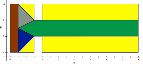
Figure 5: Reference subdomains for affine mapping

$$\boldsymbol{T}_{brown}=\begin{bmatrix}1&0\\ 0&1\end{bmatrix}\hskip 8.53581pt\boldsymbol{T}_{yellow}=\begin{bmatrix}1&0\\ 0&\frac{2}{3-w_{c}}\end{bmatrix}\hskip 8.53581pt\boldsymbol{T}_{green}=\begin{bmatrix}1&0\\ 0&\frac{1}{w_{c}}\end{bmatrix}\hskip 8.53581pt\boldsymbol{T}_{grey}=\begin{bmatrix}1&0\\ \frac{1-w_{c}}{2}&1\end{bmatrix}\hskip 8.53581pt\boldsymbol{T}_{blue}=\begin{bmatrix}1&0\\ \frac{w_{c}-1}{2}&1\end{bmatrix}\ .$$ (42)

3.2 Nonlinear Mapping

We perform the nonlinear mapping in two stages. In the first stage, a Free Form Deformation (FFD) technique is applied to the boundary points of the 2D geometry. The second stage involves moving the points in the interior of the geometry. This is accomplished using a Radial Basis Function (RBF) interpolator.

In FFD, the geometry to morph is surrounded by a box of control points, as can be seen in Fig. 6. Let $\boldsymbol{P}_{0}$ represent the set containing the original position of the control points defining the bounding box. For our particular case, the set of deformed control points’ positions $\boldsymbol{P}(\mu)$ depends on a single scalar $\mu\in[0,1]$. The deformed position $\boldsymbol{x}\in\partial\Omega$ of a point $\boldsymbol{x}_{0}\in\partial\Omega_{0}$ is then given then as,

$$\boldsymbol{x}=\text{FFD}(\boldsymbol{x}_{0},\boldsymbol{P}_{0},\boldsymbol{P}(\mu))\hskip 14.22636pt,\forall\ \boldsymbol{x}_{0}\in\partial\Omega_{0}\ ,\ \boldsymbol{x}\in\partial\Omega\ .$$ (43)

For information on the specific expression of the mappings and blending functions used, the interested reader is directed to [39, 26, 46]. We employ the implementation of FFD from the Python library PyGeM [45].

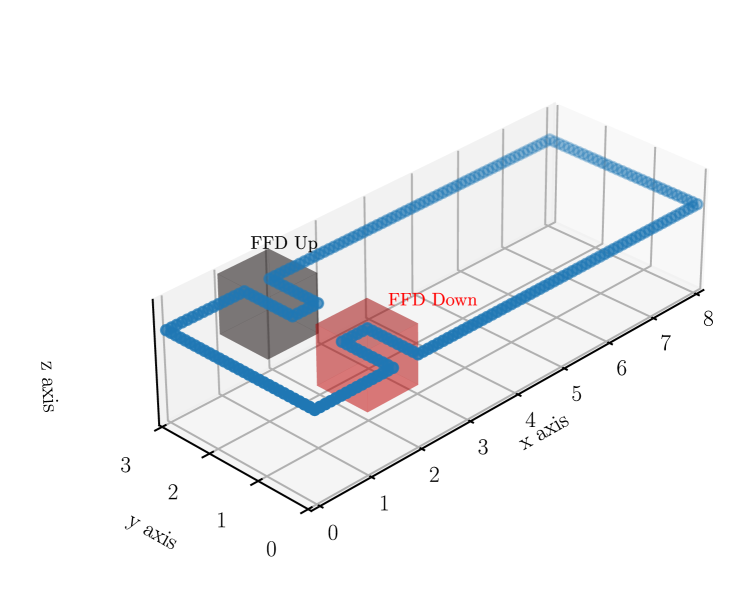
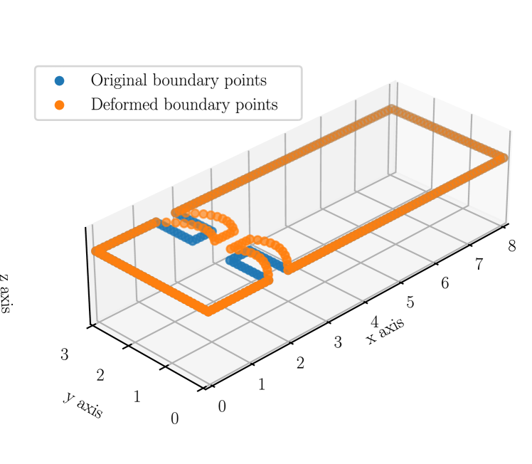
Figure 6: Free Form Deformation (FFD) part of the nonlinear mapping. For the second part of the nonlinear mapping, the interior points are moved according to a Radial Basis Function (RBF) interpolation

After the deformed boundary points have been computed, the deformed position of the points in the interior of the geometry $\boldsymbol{x}\in\Omega$ can be obtained by applying an RBF interpolator.

Let $\hat{\boldsymbol{x}}_{i}$ represent the $i$-th undeformed boundary mesh point (whose deformed position is obtained via the FFD mapping). The deformed position $\boldsymbol{x}\in\Omega$ of a point $\boldsymbol{x}_{0}\in\Omega_{0}$ is then given then as,

$$\boldsymbol{x}=\text{RBF}(\boldsymbol{x}_{0})=\sum_{i=1}^{N_{b}}\beta_{i}\phi\left(\left\lVert\boldsymbol{x}_{0}-\hat{\boldsymbol{x}}_{i}\right\rVert\right)+q(\boldsymbol{x}_{0})\ ,$$ (44)

where $N_{b}$ is the number of points in the deformed boundary, $\phi(\cdot)$ is a given basis function depending on the distance from the desired point in the interior to a mesh point in the boundary, and $q(\boldsymbol{x}_{0})$ is a polynomial. The coefficients $\beta_{i}$ and the polynomial $q(\boldsymbol{x}_{0})$, are obtained as a function of the deformed boundary points by imposing the interpolation conditions

$$\text{RBF}(\hat{\boldsymbol{x}}_{i})=\text{FFD}(\hat{\boldsymbol{x}}_{i},\boldsymbol{P}_{0},\boldsymbol{P}(\mu))\hskip 14.22636pt,\ i=1,\dots,N_{b}\ .$$ (45)

Further details about Radial Basis Functions interpolation can be found in [44, 4]. Successive application of the FFD mapping for all mesh points on the boundary of the geometry, followed by RBF parameters computation and application for all mesh points in the interior, completely defines the mapping

$$\boldsymbol{\varphi}_{\text{\tiny FFD+RBF}}: \Omega_{0}\times[0,1]\rightarrow\Omega\ ,$$ (46)

$$(\boldsymbol{x}_{0},\mu)\mapsto\boldsymbol{x}\ .$$

3.3 Mesh

The two geometric mappings require different control surfaces with a corresponding label to exist. For example, the affine mapping requires to clearly identify the coloured regions in Fig. 5 to apply the respective transformations on them. Therefore, a conforming mesh fitted to each of them was generated. On the other hand, the FFD+RBF mapping only required to identify the upper and lower rectangles defining the narrowing. For this second case, the geometry could be meshed by considering the whole geometry as a single region, while only labelling correctly the required walls. We have used unstructured meshes for both cases because they are known to work better for the specific example under consideration [36].

The bijective nature of the affine mapping allows to preserve the positive Jacobians of the isoparametric finite elements under large deformations. On the other hand, using the FFD+RBF mapping can lead to distorted finite elements which intersect, or completely swap, whenever deformations are too large. The generation of the mesh to use with the FFD+RBF mapping was chosen to be fine enough to be able to observe the desired bifurcating phenomena under a relatively large deformation, while maintaining all elements with positive Jacobians for the isoparametric transformation. For comparison purposes, the same mesh size used for the FFD+RBF mapping was also employed for the affine one.

The general purpose software KratosMultiphysics [13] was used for launching the FOM, ROM and HROM simulations, by taking advantage of the KratosRomApplication. In Kratos, the finite elements discretisation is closely linked to the physics to be simulated. For the physics in these simulations, Navier-Stokes in an Arbitrary Lagrangian Eulerian framework, the only available option was to use P1-P1 triangular elements.

The information of the meshes used can be seen in Table 1, while Figures 7, and 8 show the generated meshes.

In both figures, the presence of the probe point $p^{*}$ allows to monitor the evolution of the QoI, and therefore the occurrence of the Coanda effect. As the geometry morphs in time following a circular trajectory, a hysteresis plot can be created. The position of the probe point is selected to be located at a node in the corresponding finite element mesh that is close to the y-direction centre line, and slightly behind the narrowing.

The generation of the meshes was performed using the pre- and post-processor GiD [28].

Type of mapping	Number of Nodes	Number of Elements
Affine	2589	5147
FFD+RBF	2707	5412

Table 1: Meshes information

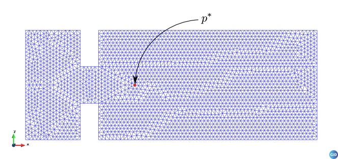
Figure 7: Finite elements mesh used for the Affine mapping. The point $p^{*}$ refers to the probe position in the mesh whose information is used for the hysteresis plot

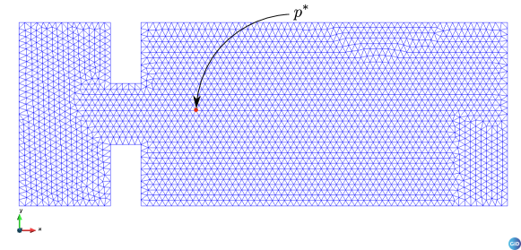
Figure 8: Finite elements mesh used for the FFD + RBF mapping. The point $p^{*}$ refers to the probe position in the mesh whose information is used for the hysteresis plot

3.4 Boundary and Initial Conditions

Both models contemplate the initial and boundary conditions shown next

$$\boldsymbol{u}=\boldsymbol{0}\ ,\ p=0\ \ ,\ \boldsymbol{x}=\begin{bmatrix}x\\ y\end{bmatrix}\in\Omega_{0}\ \ t=0\ ,$$ (47)

$$\begin{array}[]{ll}\boldsymbol{u}=\begin{bmatrix}u\\ v\end{bmatrix}&=\left\{\begin{array}[]{ll}\begin{bmatrix}y(3-y)\ sin\left(\frac{t\pi}{2}\right)\\ 0\end{bmatrix}&,x=0\ \ t=[0,1]\ ,\\ \\ \begin{bmatrix}y(3-y)\\ 0\end{bmatrix}&,x=0\ \ t=(1,T]\ ,\end{array}\right.\\ \\ p=0&\ \ \ \ ,x=8\ \ t=[0,T]\ .\end{array}$$ (48)

As can be seen, the maximum horizontal velocity at the inlet is set to 3. Moreover, the inlet velocity has been allowed to undergo an initialisation period for one second following a smooth path.

3.5 Material Properties

The values of the viscosity and density for the fluid have been selected so that, given the distortion allowed by the finite element discretisations under the respective geometric mappings, the results were qualitatively comparable to the ones reported in similar works, e.g. [36, 31, 34, 17, 18, 16]. Moreover, the material properties are held constant for all simulations.

For both models, we used the values of dynamic viscosity and density reported in the following table.

fluid property	value
dynamic viscosity $\tilde{\mu}$	0.1
density $\rho$	1.0

4 Results

In this section, we begin by providing a qualitative overview of the full order model (FOM). We present the different geometrical configurations and showcase the observed Coanda effect along with their corresponding hysteresis loops. Additionally, we offer insights into the training process of the reduced order model (ROM) and hyper-reduced order model (HROM). We discuss the testing trajectory and present the results obtained from all models. To conclude this section, we provide a quantitative comparison including error and speedup factors among the models.

The models’ files will be made available via the Examples repository of KratosMultiphysics[13] at
https://github.com/KratosMultiphysics/Examples/tree/master/rom_application/ContractionExpansionChannel.

4.1 FOM Results

Before delving into the study of the hysteresis of the Coanda effect for the contraction-expansion channel under scrutiny, we first examine the behavior of the full order model (FOM) and how variations in the geometry impact the fluid solution.

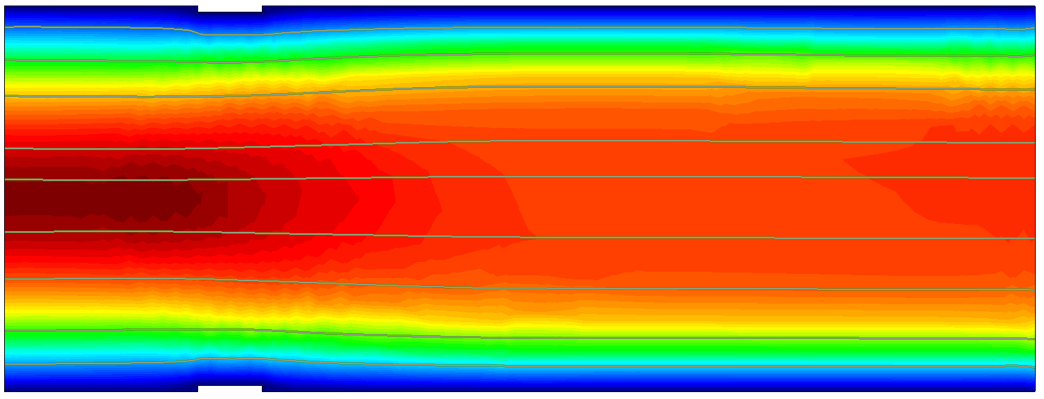
(a) $\boldsymbol{\varphi}_{\text{\tiny AFFINE}}(\cdot,2.9),\ \ w_{c}=2.9$

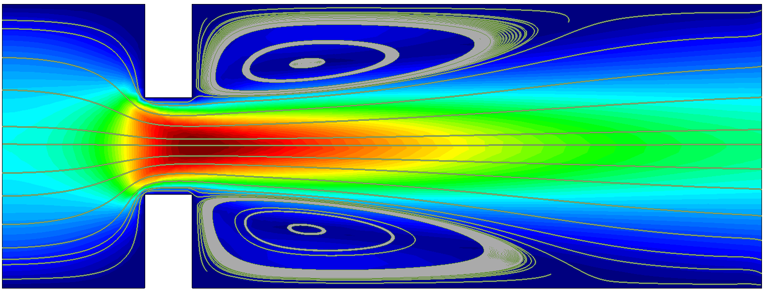
(b) $\boldsymbol{\varphi}_{\text{\tiny AFFINE}}(\cdot,1),\ \ w_{c}=1$

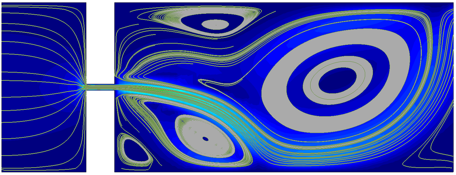
(c) $\boldsymbol{\varphi}_{\text{\tiny AFFINE}}(\cdot,0.1),\ \ w_{c}=0.1$

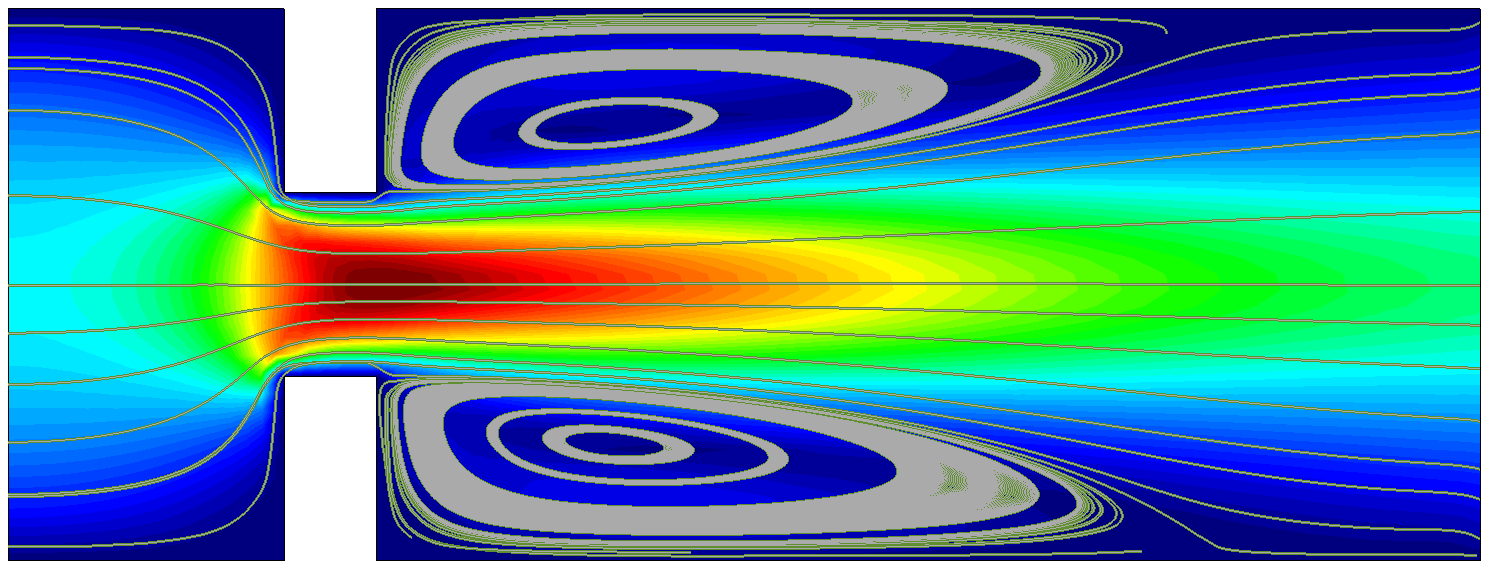
(d) $\boldsymbol{\varphi}_{\text{\tiny FFD+RBF}}(\cdot,0),\ \ w_{c}=1$

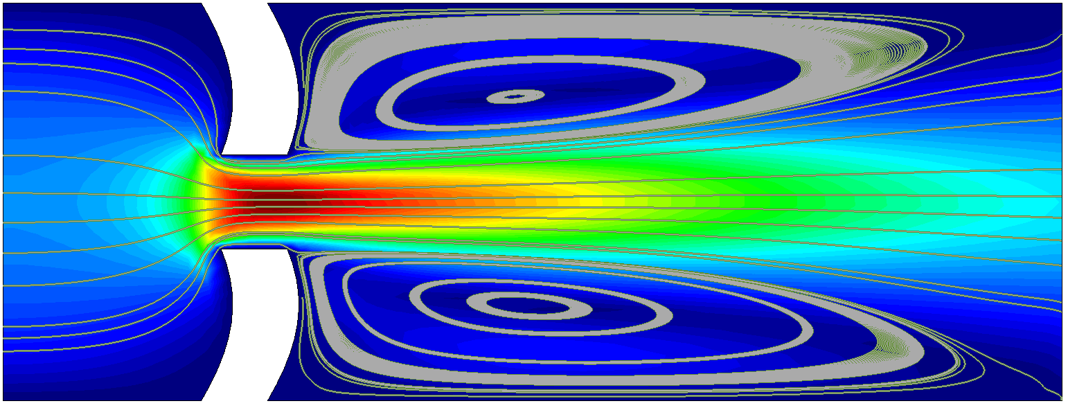
(e) $\boldsymbol{\varphi}_{\text{\tiny FFD+RBF}}(\cdot,0.5),\ \ w_{c}=0.7113$

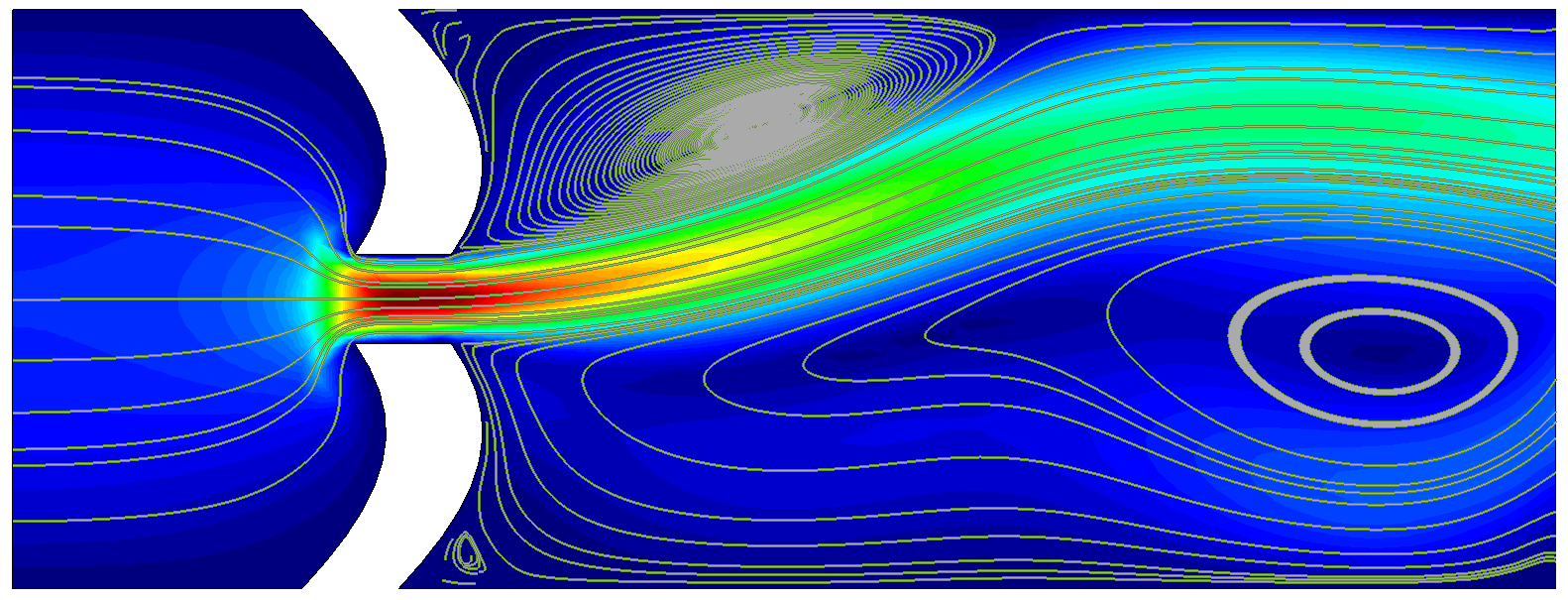
(f) $\boldsymbol{\varphi}_{\text{\tiny FFD+RBF}}(\cdot,1),\ \ w_{c}=0.422$

Figure 9: FOM solutions for different deformed configurations

Fig. 9 illustrates the flow field for extreme values of the geometric parameter $\mu$ for both the affine mapping (ranging from 0.1 to 2.9) and the FFD+RBF mapping (ranging from 0 to 1) in the contraction-expansion channel.

For the case where the narrowing width $w_{c}$ is set to 1 (Figures 9(b) and 9(d)), both mappings yield qualitatively similar solutions, characterized by a horizontally symmetric jet. However, as the narrowing width decreases, the Coanda effect becomes present, and small eddies appear on the asymmetric jets (Figures 9(c) and 9(f)).

Fig. 9(c) exhibits a complex flow pattern. Notice the relatively small value of the narrowing width made possible by the affine mapping thanks to its bijectivity. On the other hand, in Fig. 9(f), the maximum distortion allowed by employing the FFD+RBF mapping produces a narrowing width of $w_{c}=0.422$. Although this value is larger than the minimum narrowing width for the affine mapping, it still produces flow patterns relevant to the current investigation.

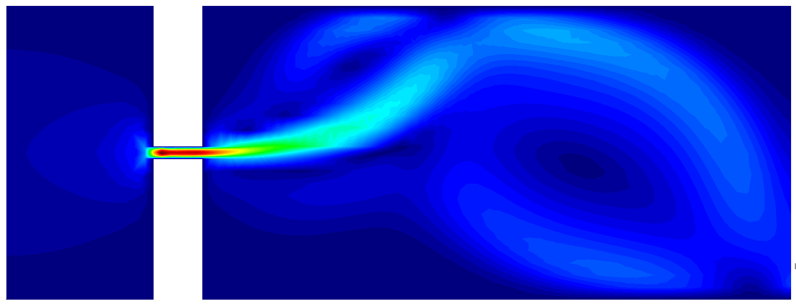
(a) $\boldsymbol{\varphi}_{\text{\tiny AFFINE}}(\cdot,0.1),\ \ w_{c}=0.1$

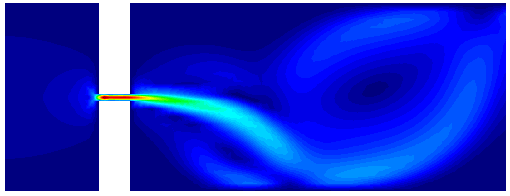
(b) $\boldsymbol{\varphi}_{\text{\tiny AFFINE}}(\cdot,0.1),\ \ w_{c}=0.1$

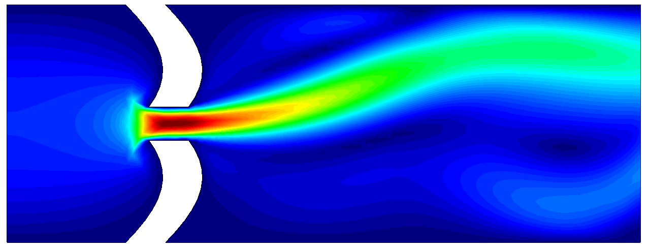
(c) $\boldsymbol{\varphi}_{\text{\tiny FFD+RBF}}(\cdot,1),\ \ w_{c}=0.422$

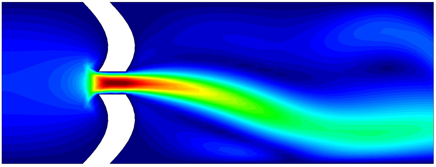
(d) $\boldsymbol{\varphi}_{\text{\tiny FFD+RBF}}(\cdot,1),\ \ w_{c}=0.422$

Figure 10: Stable solutions attach to the upper or lower walls. The symmetric jet solution is unstable and therefore not achieved

In Fig. 10, we show the possible solutions obtained for the same values of the geometric parameter $\mu$ for both mappings. Advanced methods can be used for obtaining one or the other of the stable solutions, e.g. [33]. For our specific case, we have observed that given a specific trajectory (earlier mentioned to be defined by $f_{\mu}$), that is, given an initial value of the parameter $\mu$, and then deforming the geometry in a closed loop, one of the stable solutions is obtained consistently, and a hysteresis loop can be observed.

4.1.1 Trajectories

We refer here to trajectories as the ordered set of values of the geometric parameter that define in turn a geometric morphing from an initial geometry $\Omega_{0}$, going to a maximally deformed geometry and from there back to the initial geometric configuration. For this study, two trajectories have been used. The training trajectory was used for generating the snapshots for the basis matrix $\boldsymbol{\Phi}$, as well as the hyper-reduced set of elements and weights ($\mathbb{E},\boldsymbol{\omega}$). Moreover, a testing trajectory was used for measuring the capacity of the generated ROMs to capture different geometric transformations.

In Fig. 11, the training trajectories for both mappings are shown. We keep the initial geometry static for a period of time to allow the flow to develop. Then, the morphing of the trajectory progressively makes the narrowing width $w_{c}$ arrive to a minimum value. For the case of the FFD+RBF mapping, we keep the minimum value of the narrowing width for enough time for the Coanda effect to develop. For the case of the affine mapping, the asymmetric jet is already strongly present in the solution by the time the maximum deformation is reached, therefore, for this mapping we immediately start the progressive deformation back to the initial configuration.

(a) $\boldsymbol{\varphi}_{\text{\tiny AFFINE}}(\cdot,\cdot),\ \ w_{c}\in[0.1,2.9]$

(b) $\boldsymbol{\varphi}_{\text{\tiny FFD+RBF}}(\cdot,\cdot),\ \ w_{c}\in[0.422,1]$

Figure 11: Training trajectories for both mappings

To evaluate the performance of the ROMs, we designed a specific testing trajectory for each of the considered mappings, as shown in Fig. 12. In contrast to the training trajectories, the initial and final states of the testing trajectory are swapped. This deliberate modification consistently triggers the opposite branch of the bifurcation compared to the training trajectory.

By employing this testing trajectory, we can assess the ability of the ROMs to accurately approximate simulation trajectories where the opposite branch of the bifurcation should be taken. It is expected that ROMs whose modes favor one of the branches in the bifurcation will face challenges in accurately capturing the behavior of the opposite branch. Therefore, this testing approach provides valuable insights into the performance and limitations of the ROMs in capturing the full range of system behavior.

(a) $\boldsymbol{\varphi}_{\text{\tiny AFFINE}}(\cdot,\cdot),\ \ w_{c}\in[0.1,2.9]$

(b) $\boldsymbol{\varphi}_{\text{\tiny FFD+RBF}}(\cdot,\cdot),\ \ w_{c}\in[0.422,1]$

Figure 12: Testing trajectories for both mappings

4.1.2 FOM Training Hysteresis

By monitoring the velocity on the probe point $p^{*}$ (See Fig. 7 and Fig. 8 ), we can observe the hysteresis of the velocity that this training trajectories produce, as shown in Fig 13.

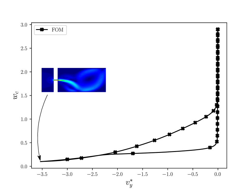
(a) $\boldsymbol{\varphi}_{\text{\tiny AFFINE}}(\cdot,\cdot),\ \ w_{c}\in[0.1,2.9]$

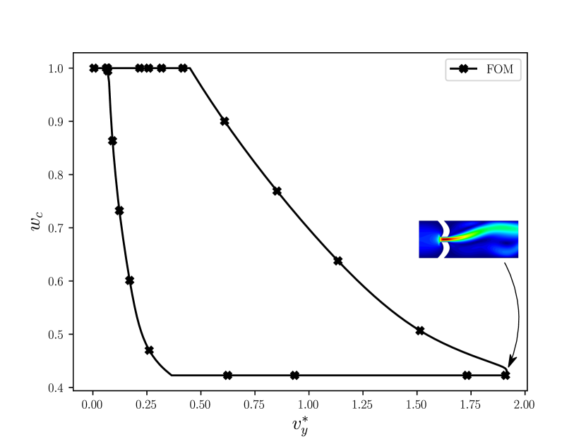
(b) $\boldsymbol{\varphi}_{\text{\tiny FFD+RBF}}(\cdot,\cdot),\ \ w_{c}\in[0.422,1]$

Figure 13: Hysteresis for the training trajectories for both mappings

As can be seen, for the training trajectories, the flow attaches to the lower wall in the case of the affine mapping, while a jet attaching to the upper wall is obtained when using the FFD+RBF mapping. These plots are to be approximated by the reduced order models, and for that purpose, can be considered the ground truth.

4.2 ROM Results

The POD procedure introduced in section 2.3.1 is applied to the snapshots matrices corresponding to the training trajectories. The singular value decay of such snapshots matrices is shown in Fig. 14. It is observed that the decay profiles of the singular values for both cases, affine mapping and nonlinear mapping, are similar. This similarity can be attributed to the fact that the flow properties and the employed meshes are comparable in both cases.

The larger number of singular values for the affine mapping compared to the nonlinear mapping arises from the smaller time step required by the model with the affine mapping, particularly when the narrowing width $w_{c}$ was at its minimum.

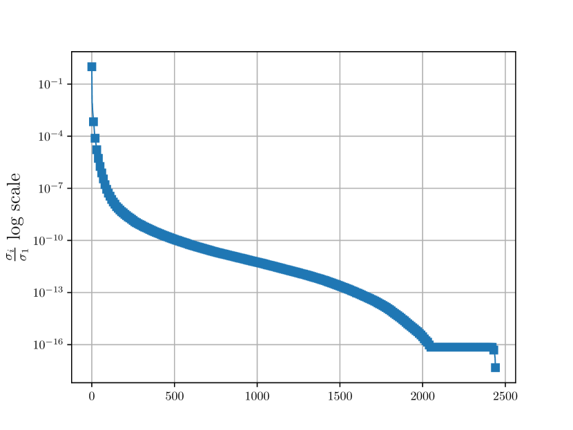
(a) $\boldsymbol{\varphi}_{\text{\tiny AFFINE}}(\cdot,\cdot),\ \ w_{c}\in[0.1,2.9]$

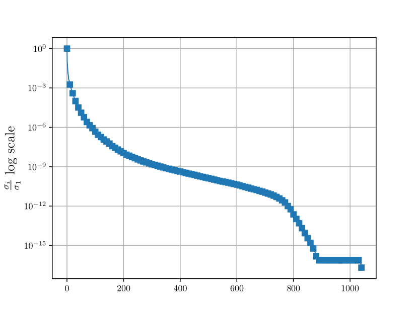
(b) $\boldsymbol{\varphi}_{\text{\tiny FFD+RBF}}(\cdot,\cdot),\ \ w_{c}\in[0.422,1]$

Figure 14: Singular values decay for the training trajectories for both mappings

In this study we have explored four different truncation tolerances for the SVD of the snapshots matrices (we use a subscript SOL referring to the solution vector, in order to differentiate it from the snapshots of the residual projected present during the hyper-reduction). In particular $\epsilon_{\text{\tiny SOL}}=\{1e-3,1e-4,1e-5,1e-6\}$, such that

$$\left\lVert\boldsymbol{S}-\boldsymbol{\Phi}\boldsymbol{\Phi}^{T}\boldsymbol{S}\right\rVert_{F}\leq\epsilon_{\text{\tiny SOL}}\left\lVert\boldsymbol{S}\right\rVert_{F}\ ,$$ (49)

where $\boldsymbol{S}$ is the snapshots matrix and $\left\lVert\cdot\right\rVert_{F}$ is the Frobenius norm. The leading velocity and pressure modes for the affine mapping are shown in Fig. 15, while the leading modes for the FFD+RBF mapping are shown in Fig. 16.

4.2.1 Selected Modes

The modes obtained for the affine mapping, in terms of velocity and pressure, exhibit a tendency for the asymmetric jet to bend towards the lower wall. This behavior is reflected in the dominant flow patterns captured by these modes.

On the other hand, the modes obtained for the FFD+RBF mapping exhibit a preference for the upper wall. These modes capture the flow patterns where the jet tends to attach to the upper wall of the channel.

The different modes obtained for each mapping highlight the distinct flow characteristics and behaviors induced by the geometric deformations in the training trajectories.

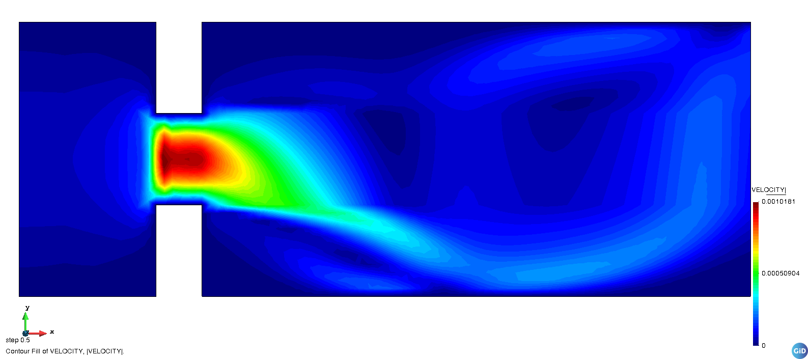
(a) velocity mode 1

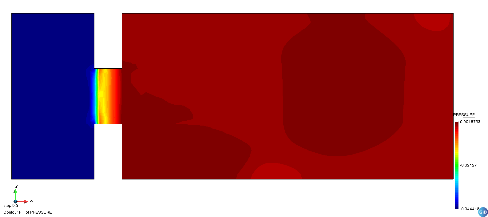
(b) pressure mode 1

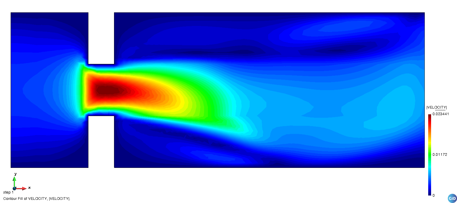
(c) velocity mode 2

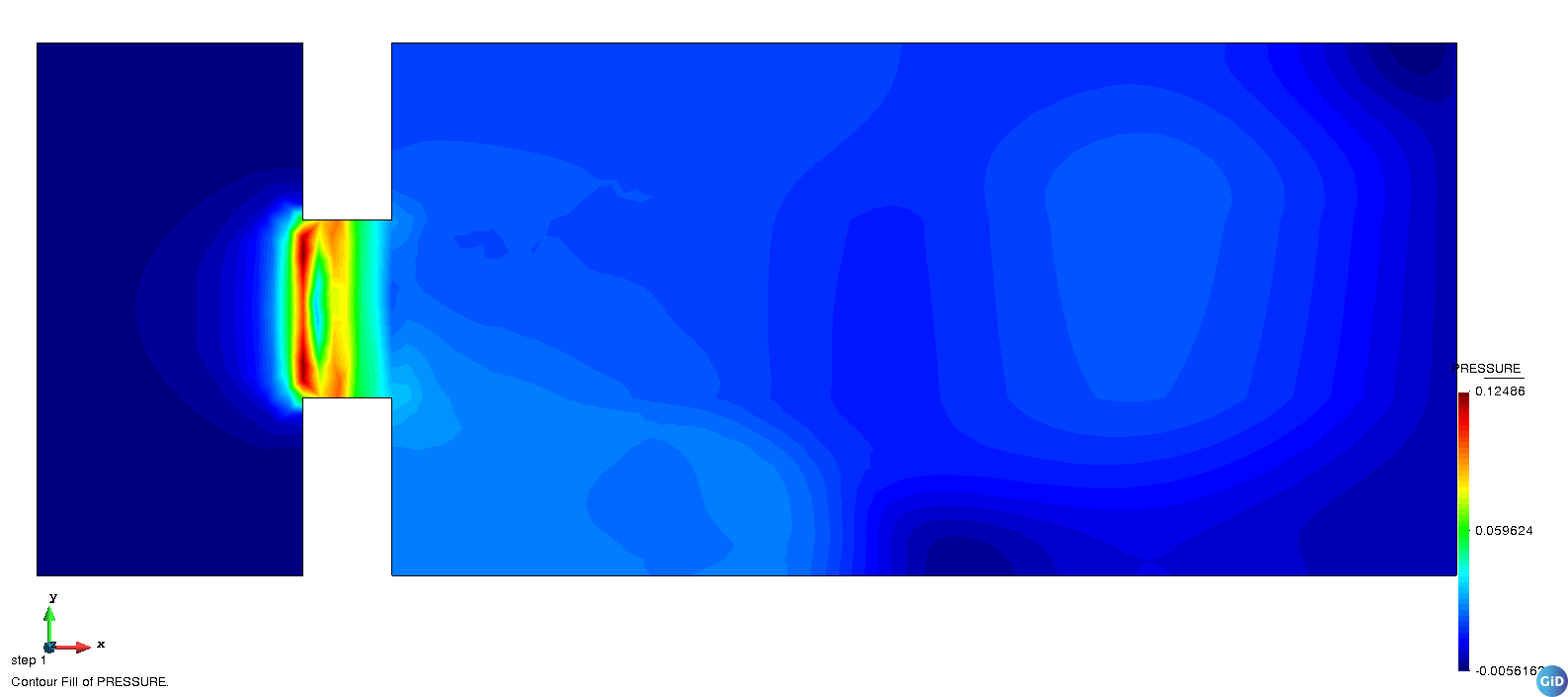
(d) pressure mode 2

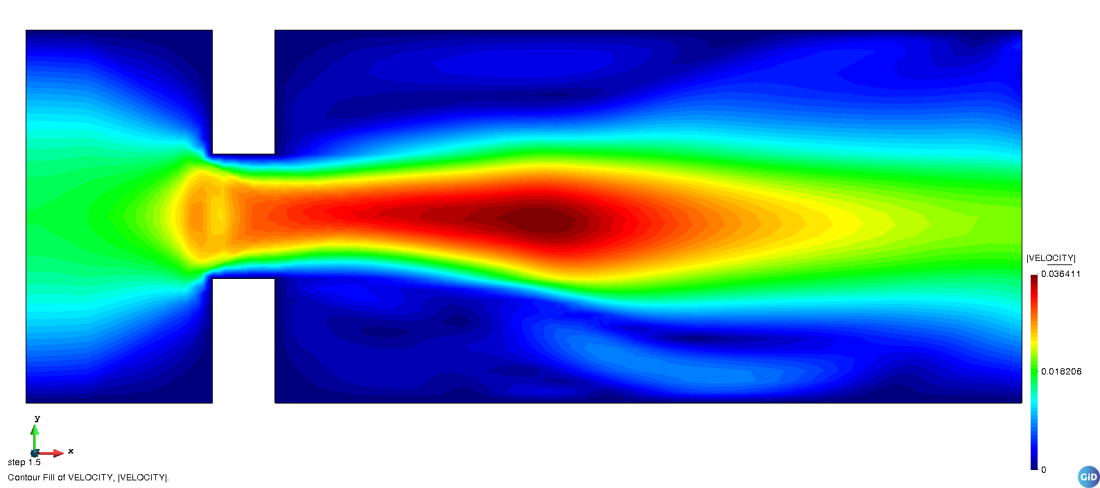
(e) velocity mode 3

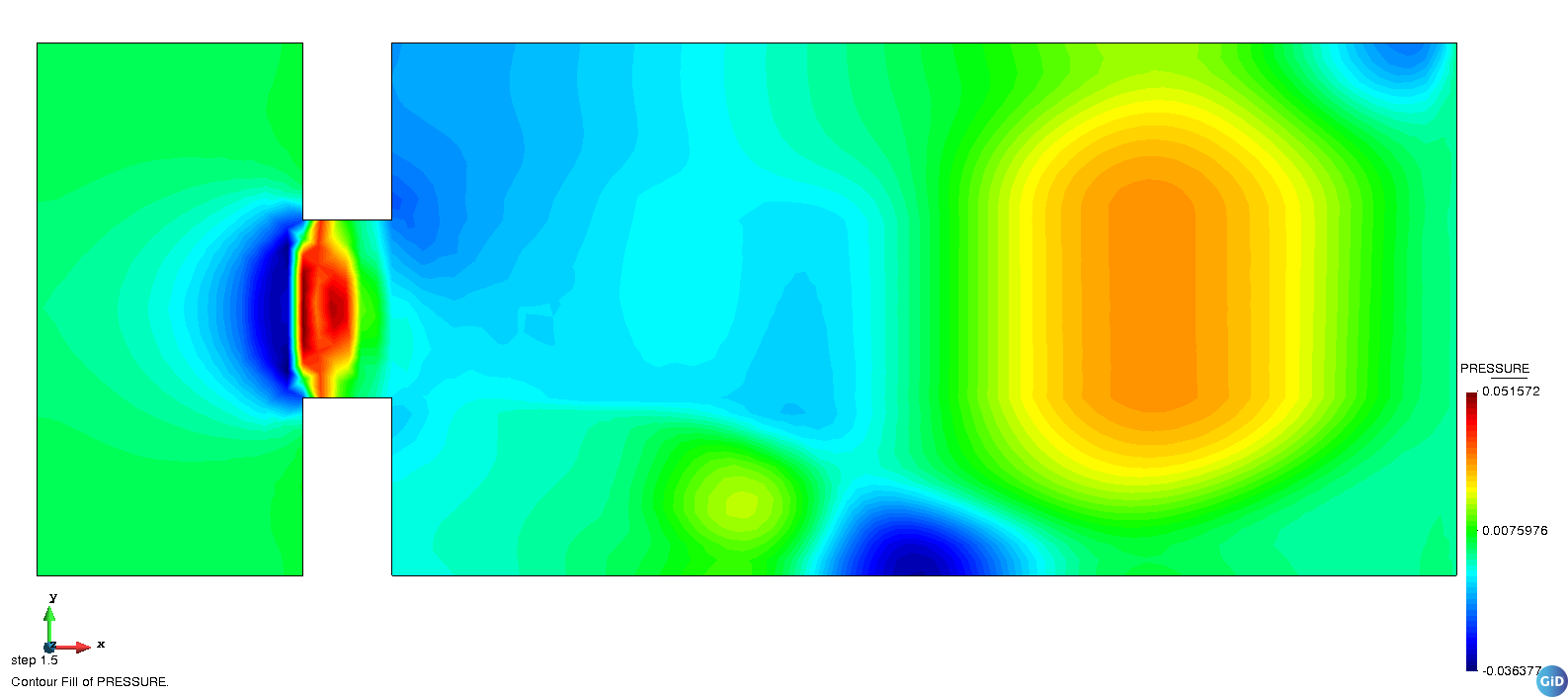
(f) pressure mode 3

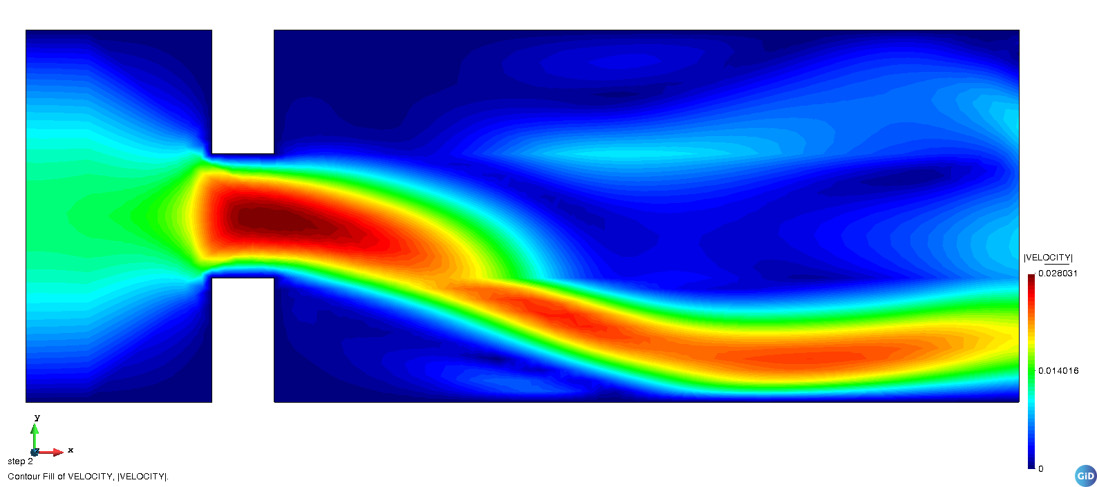
(g) velocity mode 4

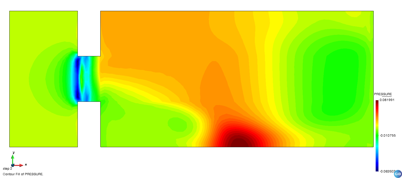
(h) pressure mode 4

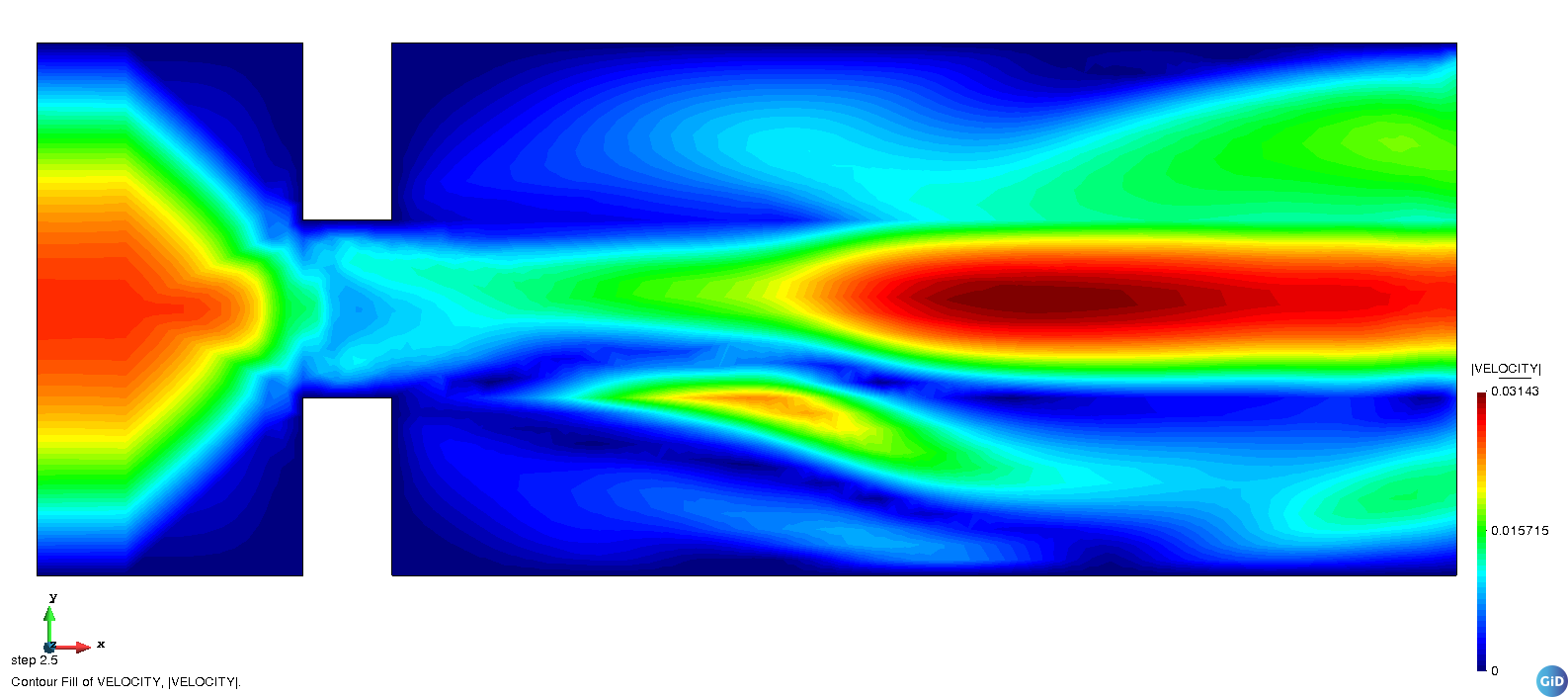
(i) velocity mode 5

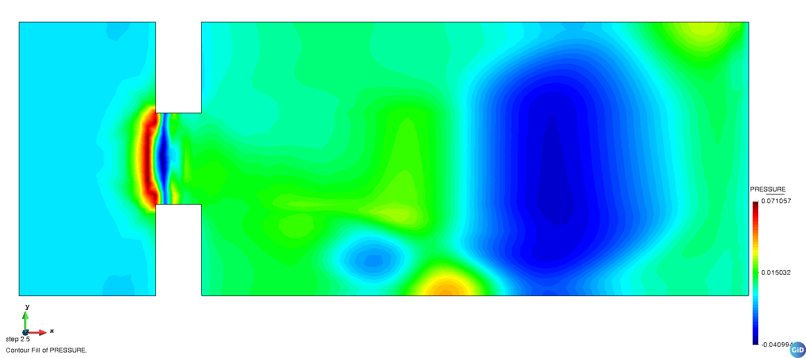
(j) pressure mode 5

Figure 15: First five velocity and pressure modes for the $\boldsymbol{\varphi}_{\text{\tiny AFFINE}}$ mapping

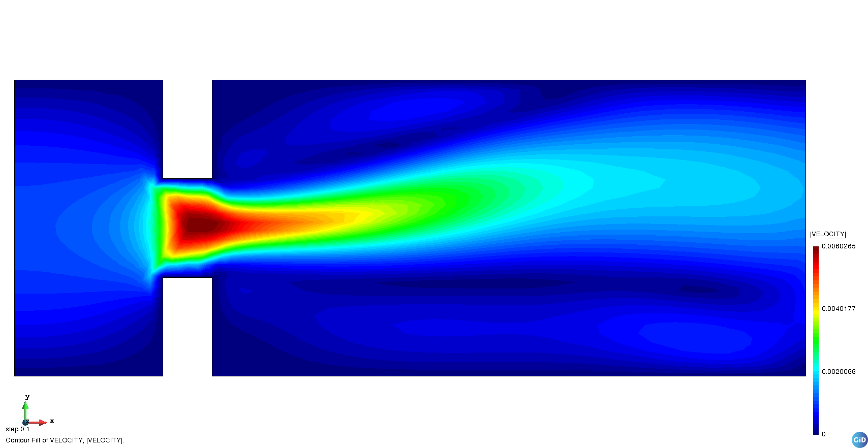
(a) velocity mode 1

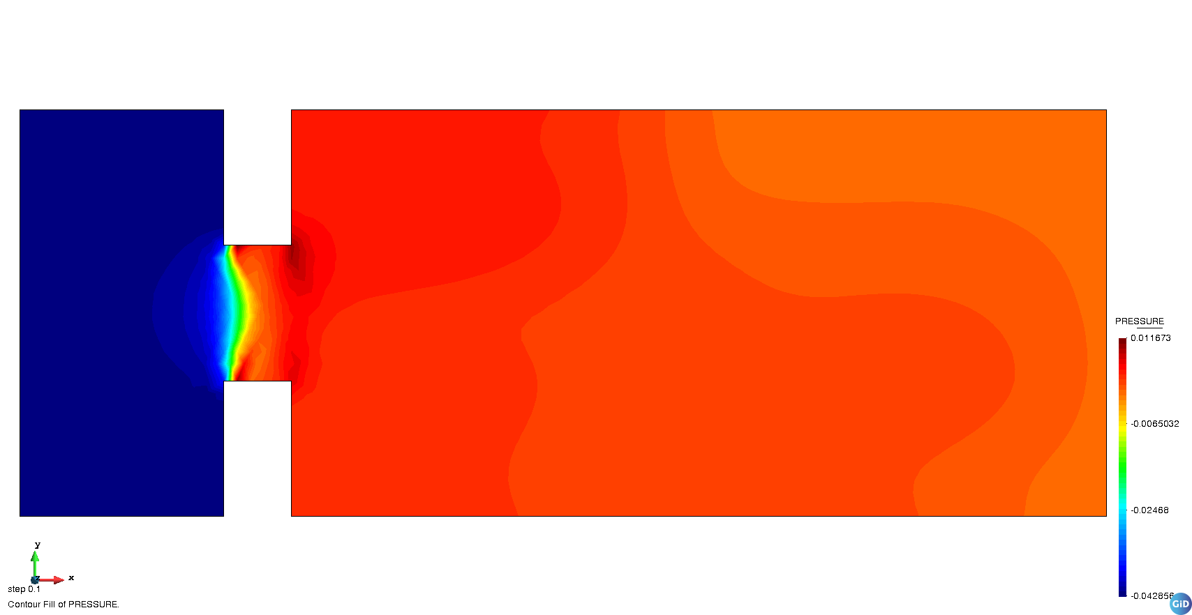
(b) pressure mode 1

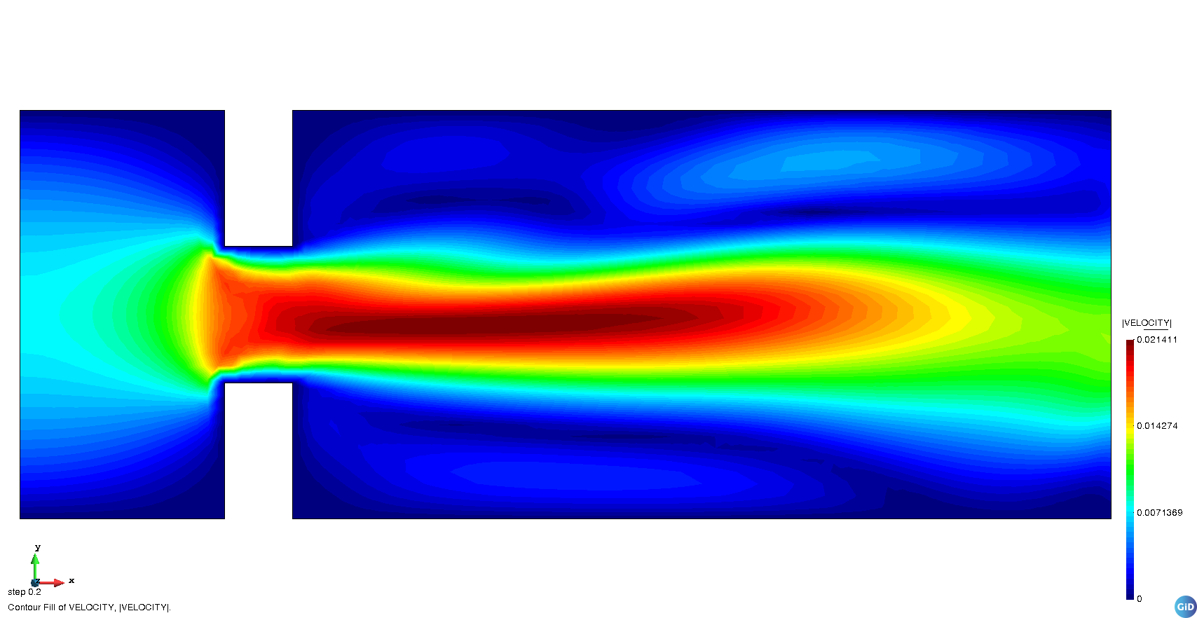
(c) velocity mode 2

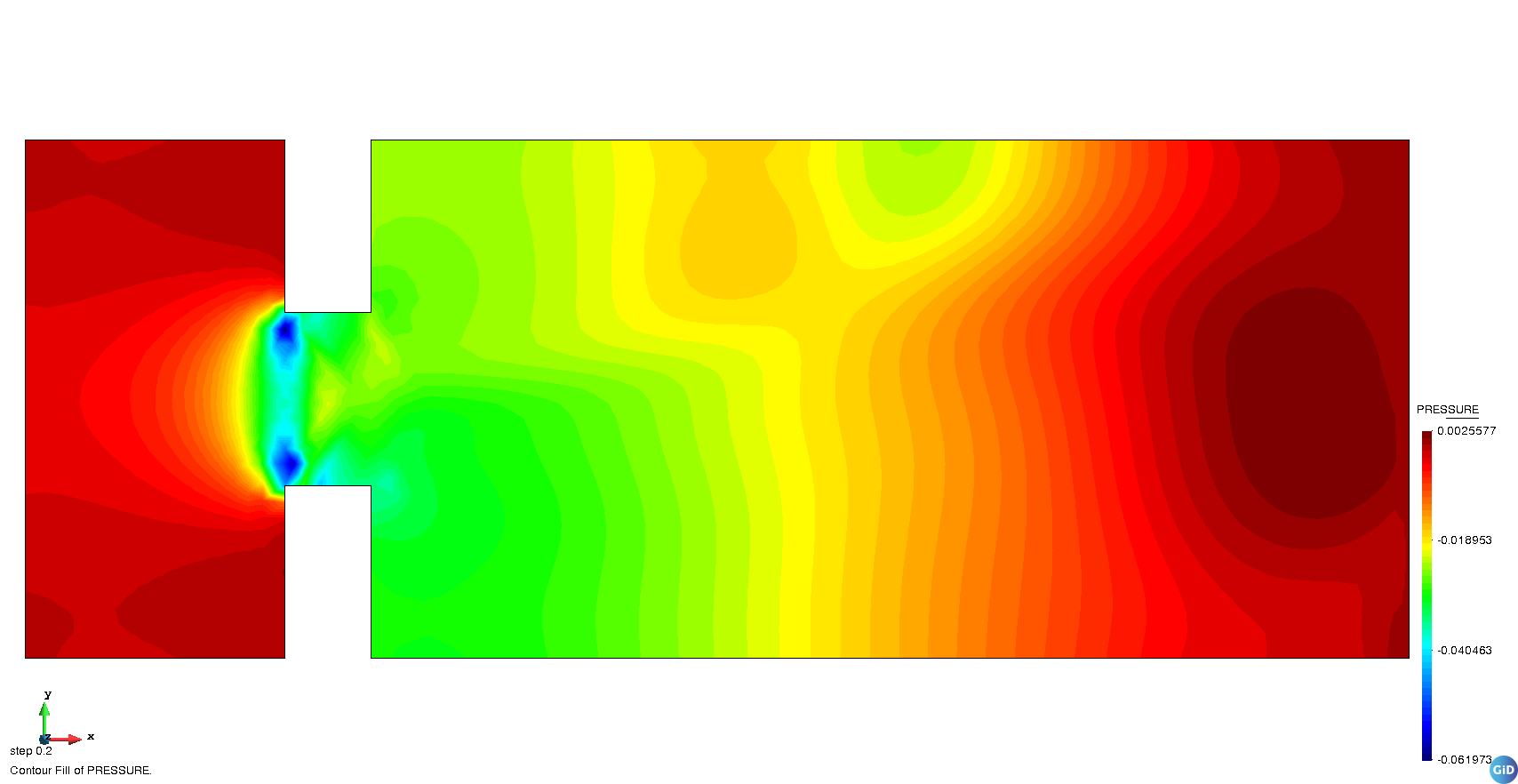
(d) pressure mode 2

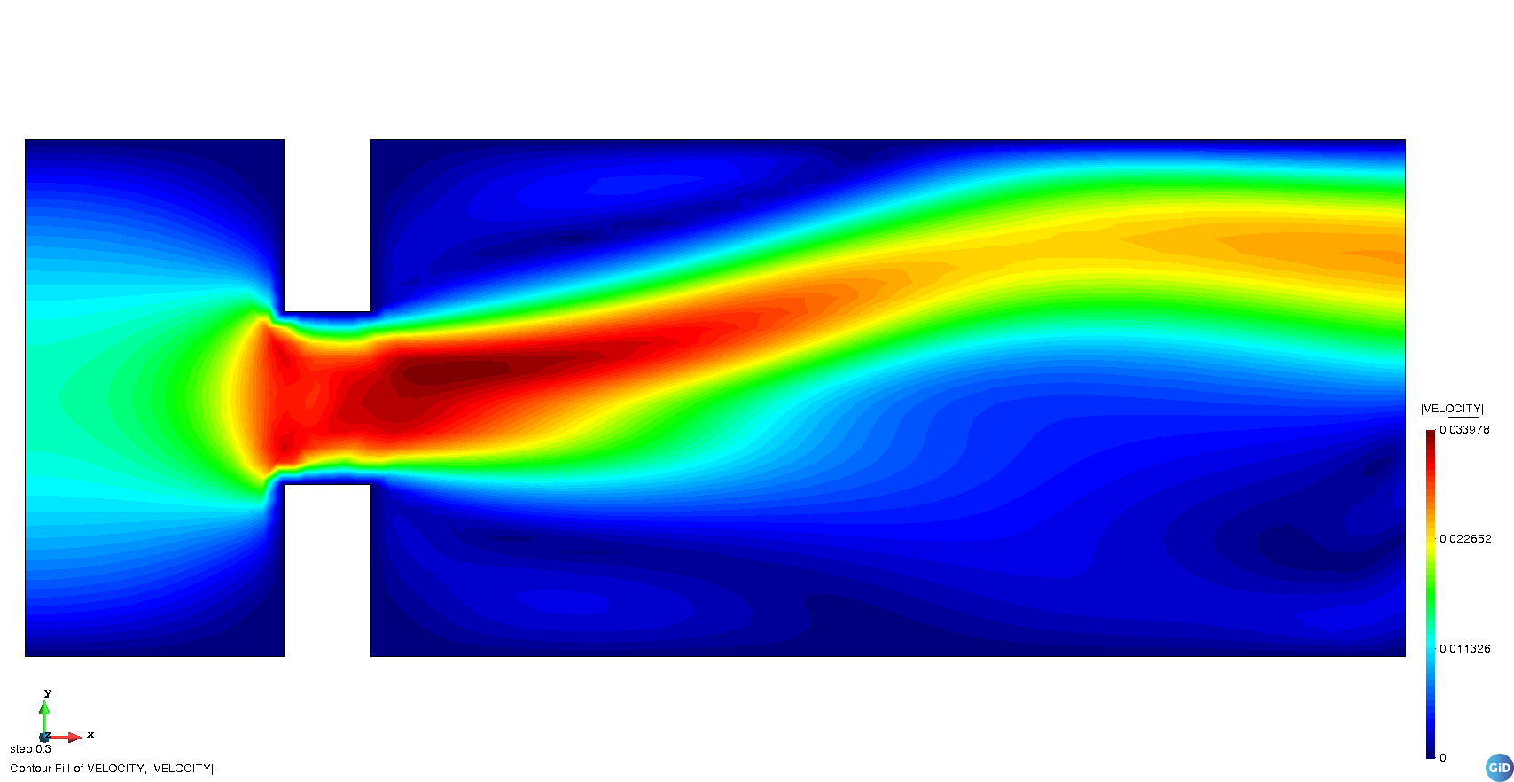
(e) velocity mode 3

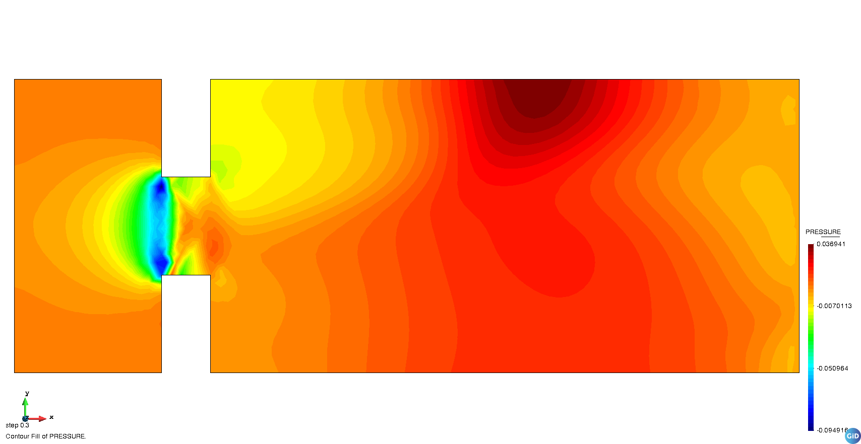
(f) pressure mode 3

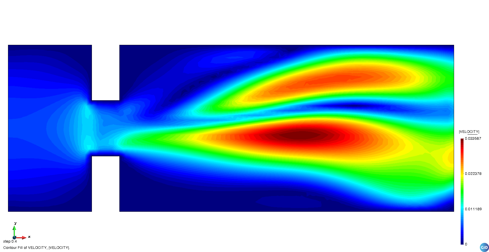
(g) velocity mode 4

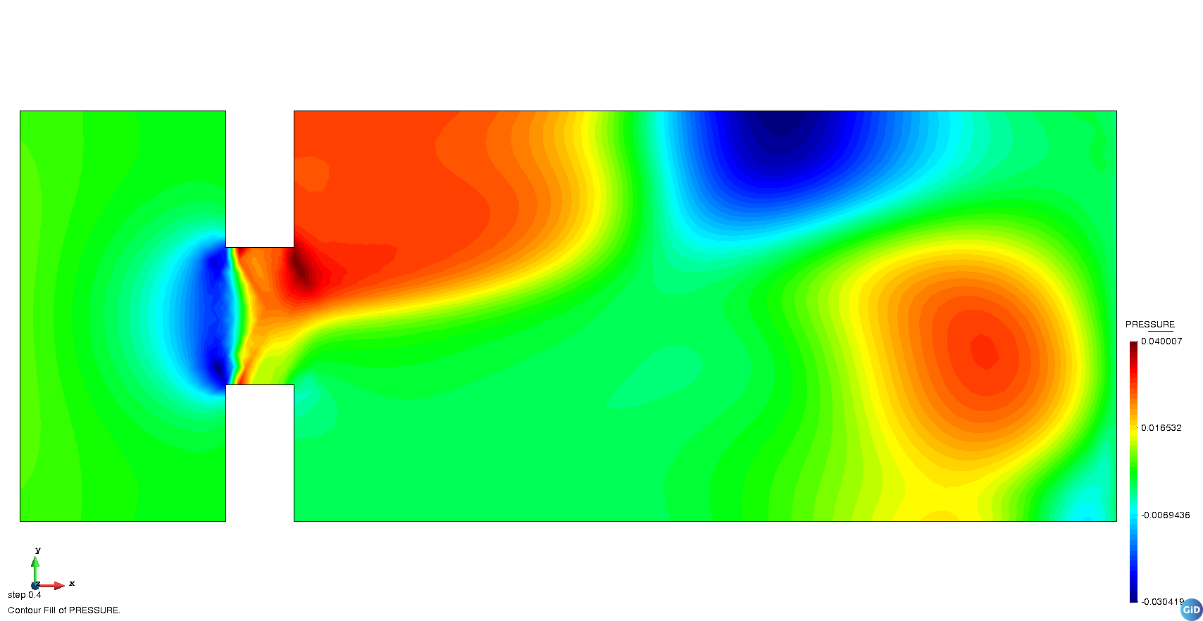
(h) pressure mode 4

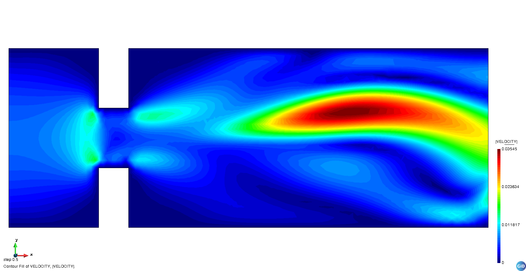
(i) velocity mode 5

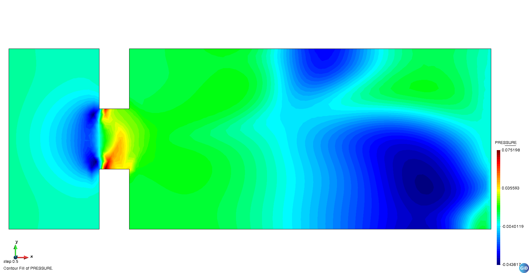
(j) pressure mode 5

Figure 16: First five velocity and pressure modes for the $\boldsymbol{\varphi}_{\text{\tiny FFD+RBF}}$ mapping

4.2.2 FOM vs ROM hysteresis for training trajectory

The Reduced Order Model of the training trajectory was launched taking the required amount of modes to comply with the truncation tolerance $\epsilon_{\text{\tiny SOL}}$. The results in the phase-space for the quantity of interest $v_{y}^{*}$ are shown in Fig. 17.

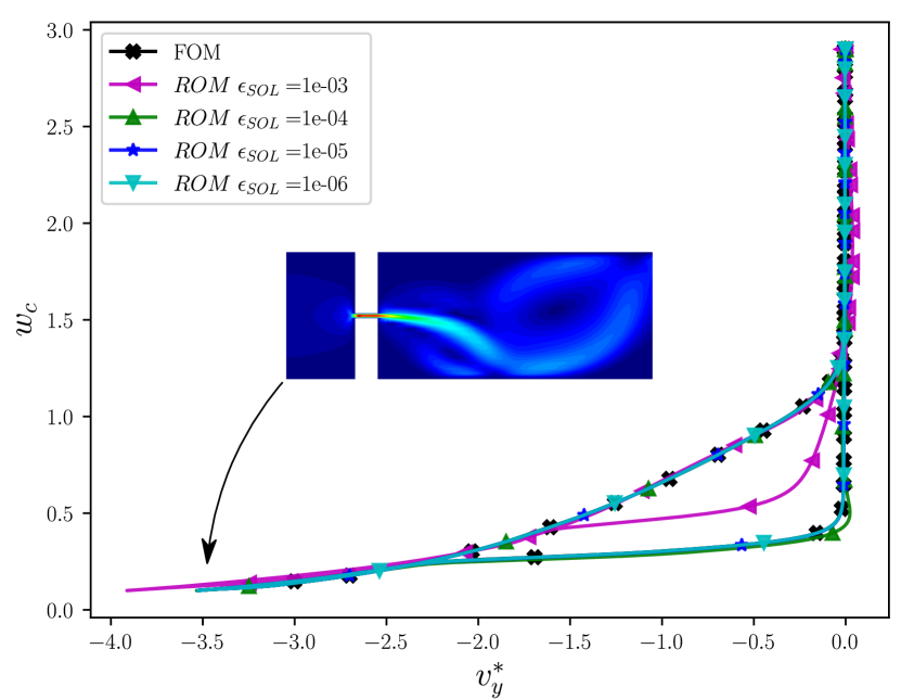
(a) $\boldsymbol{\varphi}_{\text{\tiny AFFINE}}(\cdot,\cdot),\ \ w_{c}\in[0.1,2.9]$

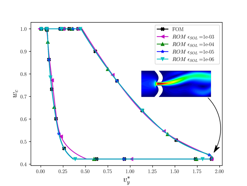
(b) $\boldsymbol{\varphi}_{\text{\tiny FFD+RBF}}(\cdot,\cdot),\ \ w_{c}\in[0.422,1]$

Figure 17: FOM vs ROM hysteresis for the training trajectories for both mappings

The behavior of the Coanda effect is accurately captured when reconstructing the training trajectory using the reduced order model (ROM) for all the considered truncation tolerances. However, it is observed that the ROM solution with a truncation tolerance of $\epsilon_{\text{\tiny SOL}}=1e-3$ deviates considerably from the solutions of the other models, in particular for the affine mapping, and less so for the FFD+RBF mapping.

This discrepancy suggests that a higher truncation tolerance leads to a loss of accuracy in reproducing the Coanda effect phenomenon. Therefore, it is important to choose an appropriate truncation tolerance to ensure reliable and accurate ROM predictions of the Coanda effect behavior.

4.2.3 FOM vs ROM hysteresis for testing trajectory for both mappings

Fig. 18 presents the testing trajectory plots, illustrating a comparison between the full order model (FOM) solution and the reduced order model (ROM) solutions for each truncation tolerance and both mappings.

In the case of the affine mapping, none of the truncation tolerances yield a basis capable of accurately reproducing the FOM trend in the Coanda effect. The ROMs constructed with the affine mapping fail to capture the correct branch of the bifurcation.

On the other hand, for the FFD+RBF mapping, only the ROM constructed with a tolerance of $\epsilon_{\text{\tiny RES}}=1e-3$ deviates to take the ”wrong” branch of the bifurcation. The remaining ROMs show an improved performance compared to the affine mapping case. Although none of the ROMs perfectly match the FOM solution, they progressively approach it.

These results highlight the challenges of accurately capturing the Coanda effect and its hysteresis behavior using reduced order models, especially when dealing with testing trajectories that require capturing the behavior of the opposite branch of the bifurcation.

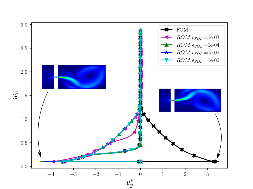
(a) $\boldsymbol{\varphi}_{\text{\tiny AFFINE}}(\cdot,\cdot),\ \ w_{c}\in[0.1,2.9]$

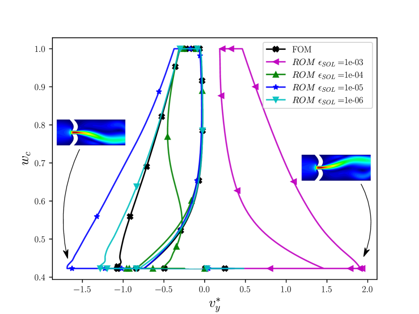
(b) $\boldsymbol{\varphi}_{\text{\tiny FFD+RBF}}(\cdot,\cdot),\ \ w_{c}\in[0.422,1]$

Figure 18: FOM vs ROM hysteresis for the testing trajectory for both mappings

4.3 HROM

In order to obtain a more efficient reduced order model, we developed a hyper-reduced order model (HROM) by projecting the residual onto the corresponding solution basis as exposed in section 2.3.2. The process involved taking the SVD of the matrix of projected residuals, denoted as $\boldsymbol{S}_{r}$. The truncation tolerances chosen for $\boldsymbol{S}r$ were $\epsilon_{\text{\tiny RES}}=\{1e-3,1e-4,1e-5,1e-6\}$, satisfying the condition:

$$\left\lVert\boldsymbol{S}_{r}-\boldsymbol{G}^{T}\boldsymbol{G}\boldsymbol{S}_{r}\right\rVert_{F}\leq\epsilon_{\text{\tiny RES}}\left\lVert\boldsymbol{S}_{r}\right\rVert_{F}\ .$$ (50)

Here, the matrix $\boldsymbol{G}(\boldsymbol{R},\boldsymbol{\Phi})$ represents a basis for the row space of the projected residuals matrix. The Empirical Cubature Method (ECM) algorithm [15, 14] was then applied to obtain the selected hyper-reduced elements and their corresponding positive weights:

$$(\mathbb{E},\boldsymbol{\omega})=\texttt{ECM}(\boldsymbol{G})\ .$$ (51)

Empirical observations have shown that the total number of selected elements is proportional to the number of modes in the POD basis

$$\dim(\mathbb{E})\propto\dim(\boldsymbol{\Phi})\ .$$ (52)

Based on experience, a rule of thumb has been developed to estimate the number of selected elements as the square of the number of modes in the solution basis. For some structural mechanics problems, this claim can be shown. For other physical problems, this rule of thumb provides a useful guideline for estimating the number of selected elements in the HROM.

4.3.1 Selected HROM elements

Figures 19 and 20 display the finite element meshes for both the affine mapping and FFD+RBF mapping, highlighting the selected HROM elements for all the combinations of the studied tolerances $\epsilon_{\text{\tiny SOL}}$ and $\epsilon_{\text{\tiny RES}}$. It can be observed that as the tolerances become smaller, the number of selected elements increases, and they tend to accumulate in regions that match the patterns present in the corresponding modes (as shown in Figures 16 and 15). Specifically, the selected elements concentrate in the narrowing area and either the lower or upper walls, depending on which branch of the bifurcation was preferred during the corresponding training trajectories.

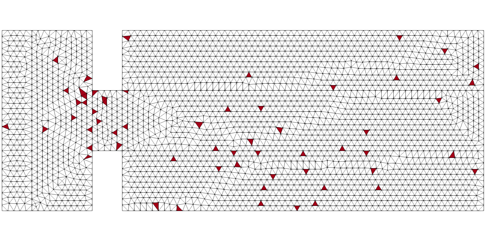
(a) $\epsilon_{\text{\tiny SOL}}=1e-3,\epsilon_{\text{\tiny RES}}=1e-3,$

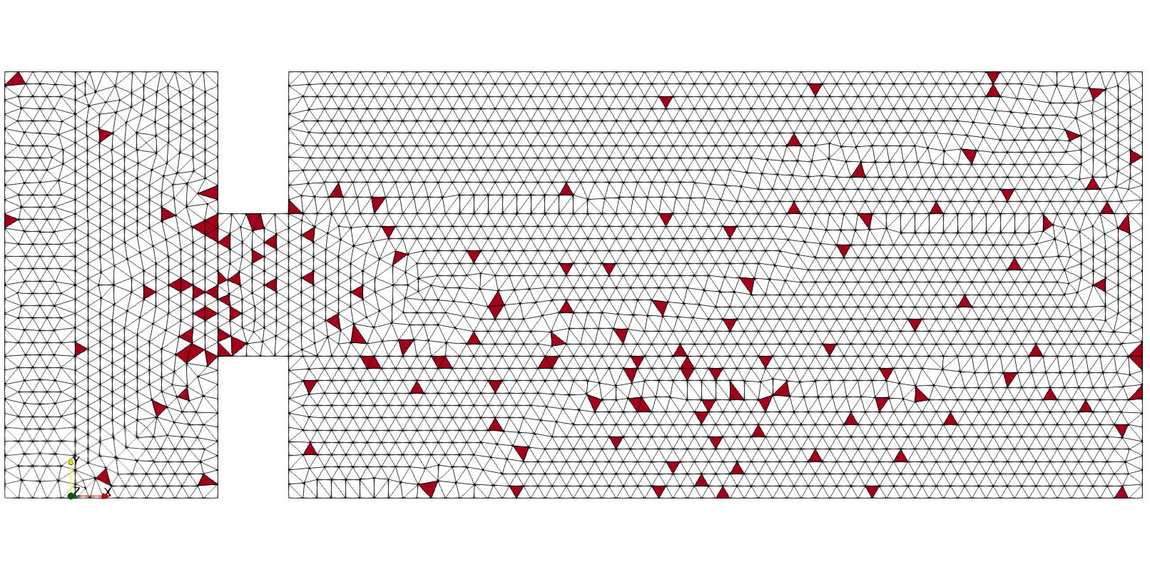
(b) $\epsilon_{\text{\tiny SOL}}=1e-3,\epsilon_{\text{\tiny RES}}=1e-4,$

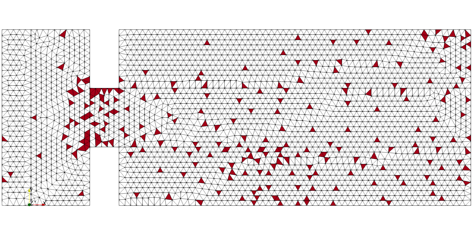
(c) $\epsilon_{\text{\tiny SOL}}=1e-3,\epsilon_{\text{\tiny RES}}=1e-5,$

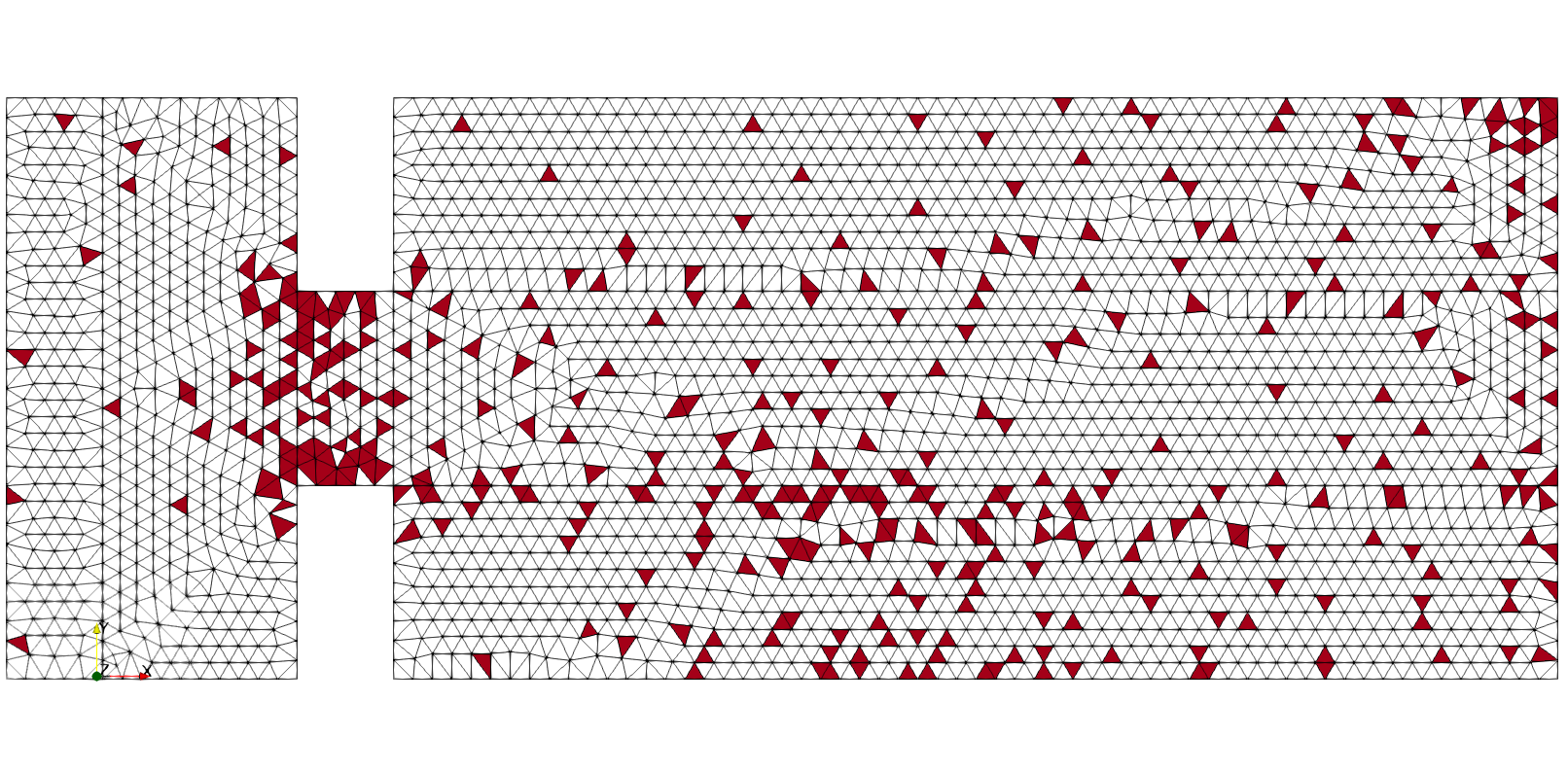
(d) $\epsilon_{\text{\tiny SOL}}=1e-3,\epsilon_{\text{\tiny RES}}=1e-6,$

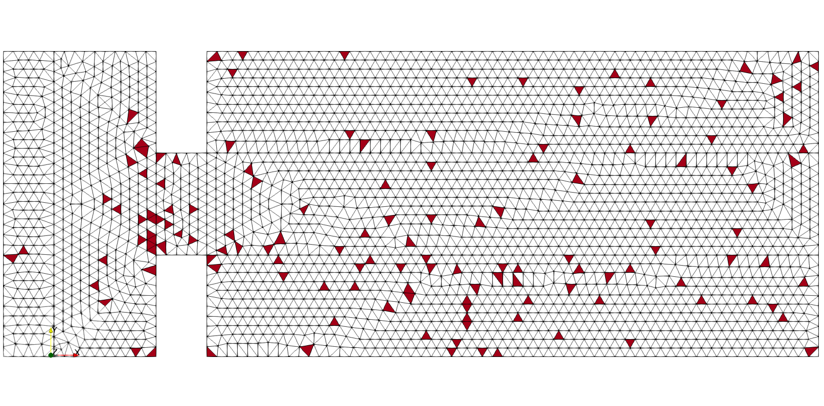
(e) $\epsilon_{\text{\tiny SOL}}=1e-4,\epsilon_{\text{\tiny RES}}=1e-3,$

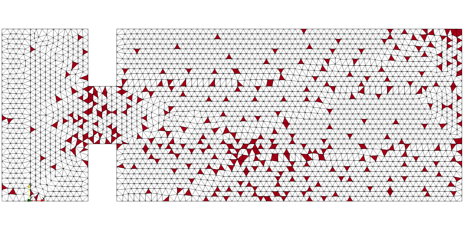
(f) $\epsilon_{\text{\tiny SOL}}=1e-4,\epsilon_{\text{\tiny RES}}=1e-4,$

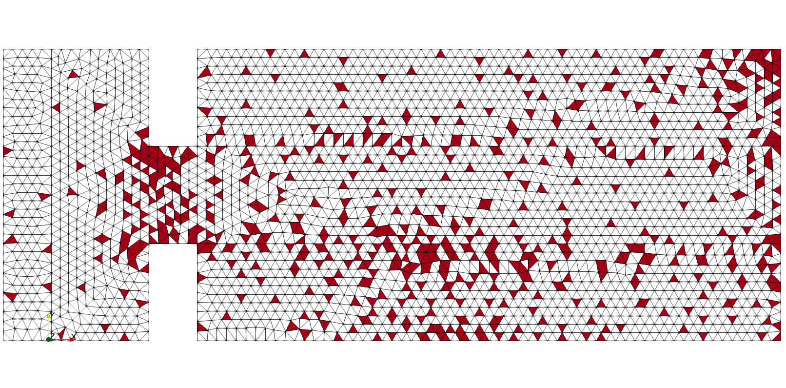
(g) $\epsilon_{\text{\tiny SOL}}=1e-4,\epsilon_{\text{\tiny RES}}=1e-5,$

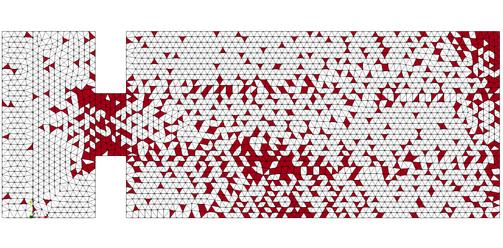
(h) $\epsilon_{\text{\tiny SOL}}=1e-4,\epsilon_{\text{\tiny RES}}=1e-6,$

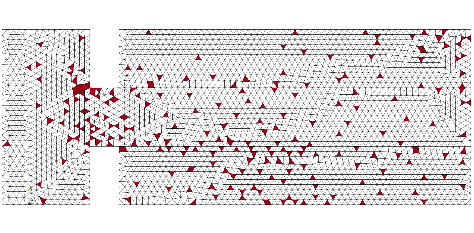
(i) $\epsilon_{\text{\tiny SOL}}=1e-5,\epsilon_{\text{\tiny RES}}=1e-3,$

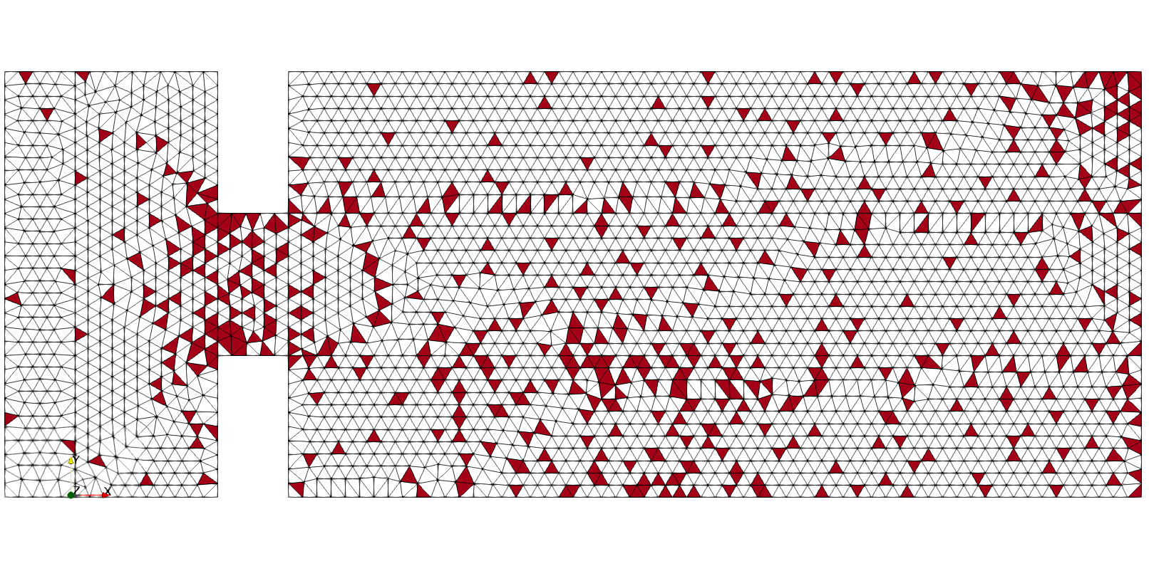
(j) $\epsilon_{\text{\tiny SOL}}=1e-5,\epsilon_{\text{\tiny RES}}=1e-4,$

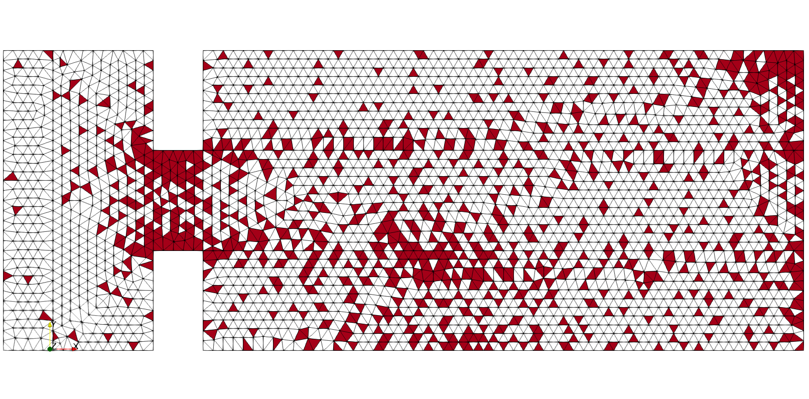
(k) $\epsilon_{\text{\tiny SOL}}=1e-5,\epsilon_{\text{\tiny RES}}=1e-5,$

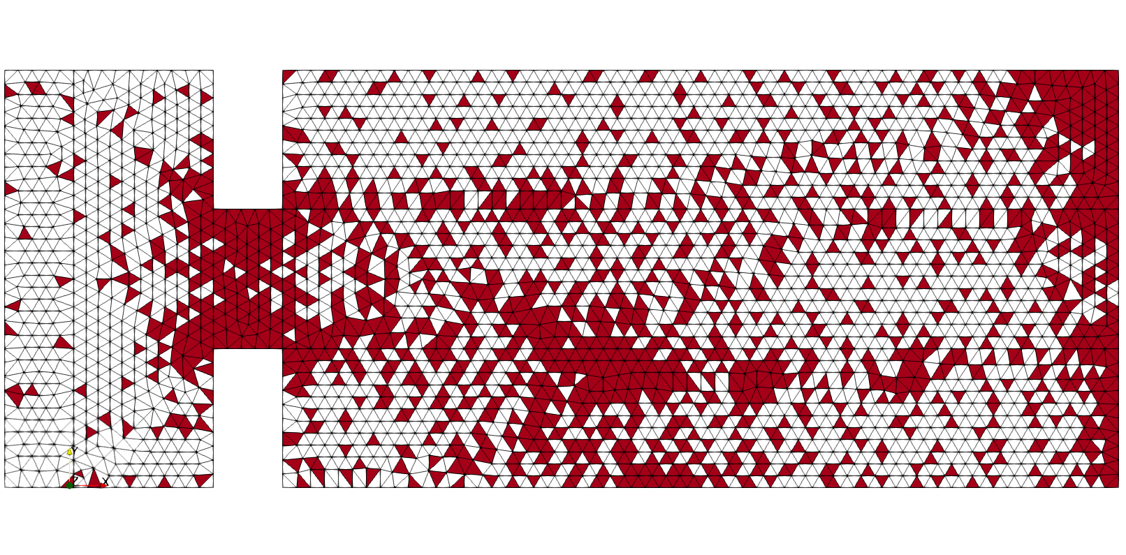
(l) $\epsilon_{\text{\tiny SOL}}=1e-5,\epsilon_{\text{\tiny RES}}=1e-6,$

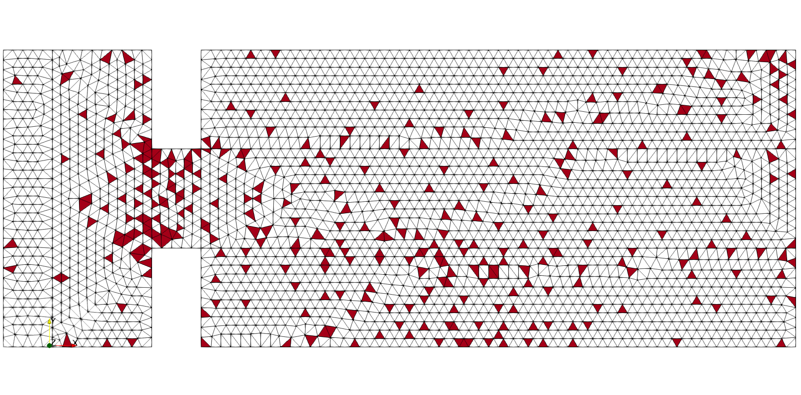
(m) $\epsilon_{\text{\tiny SOL}}=1e-6,\epsilon_{\text{\tiny RES}}=1e-3,$

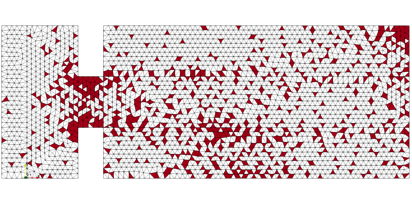
(n) $\epsilon_{\text{\tiny SOL}}=1e-6,\epsilon_{\text{\tiny RES}}=1e-4,$

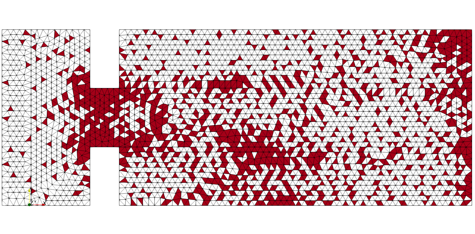
(o) $\epsilon_{\text{\tiny SOL}}=1e-6,\epsilon_{\text{\tiny RES}}=1e-5,$

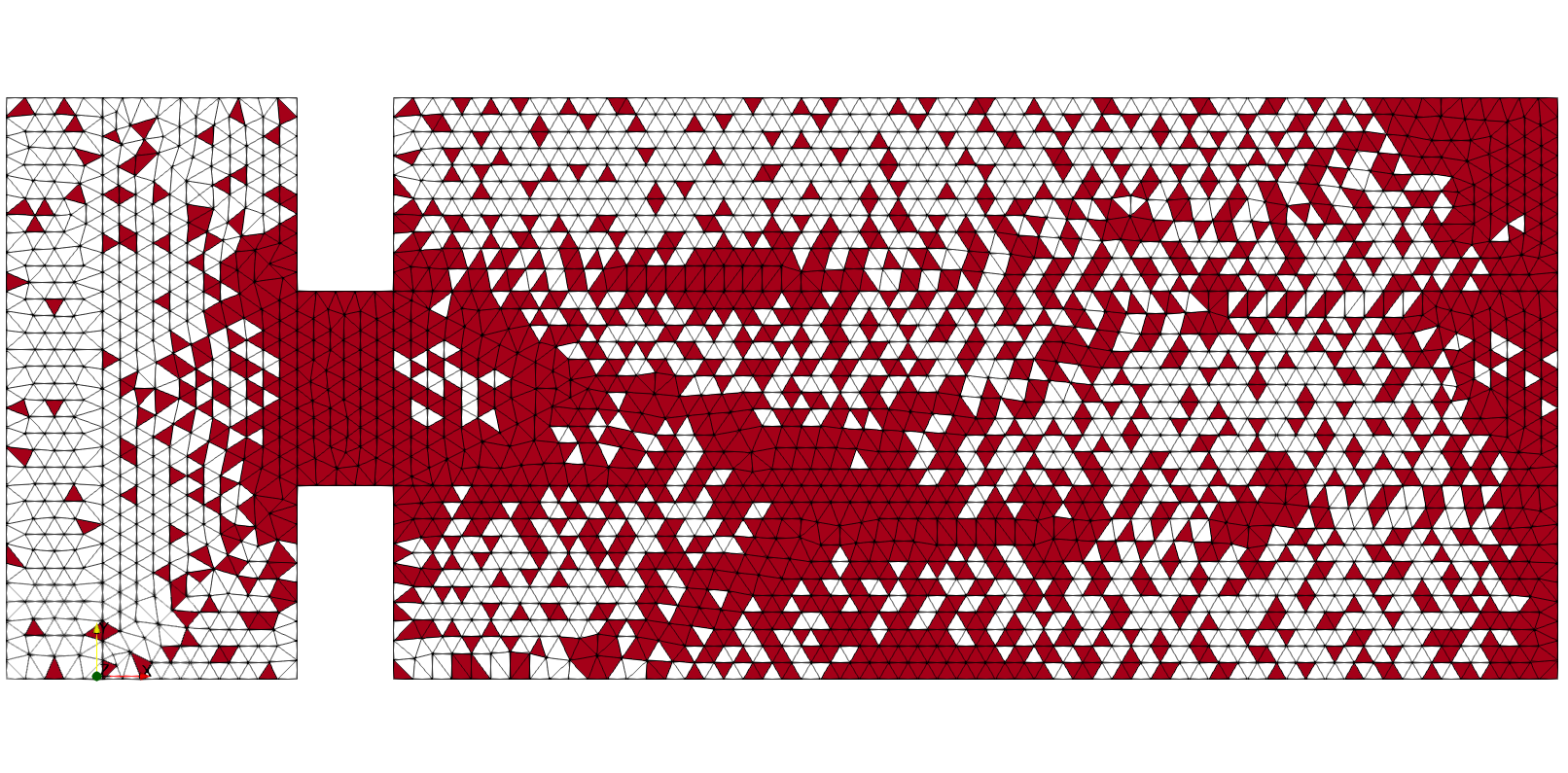
(p) $\epsilon_{\text{\tiny SOL}}=1e-6,\epsilon_{\text{\tiny RES}}=1e-6,$

Figure 19: Hyper-reduced elements selected for $\boldsymbol{\varphi}_{\text{\tiny AFFINE}}$

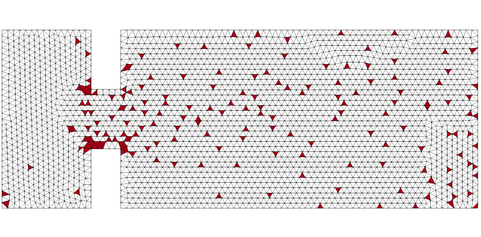
(a) $\epsilon_{\text{\tiny SOL}}=1e-3,\epsilon_{\text{\tiny RES}}=1e-3,$

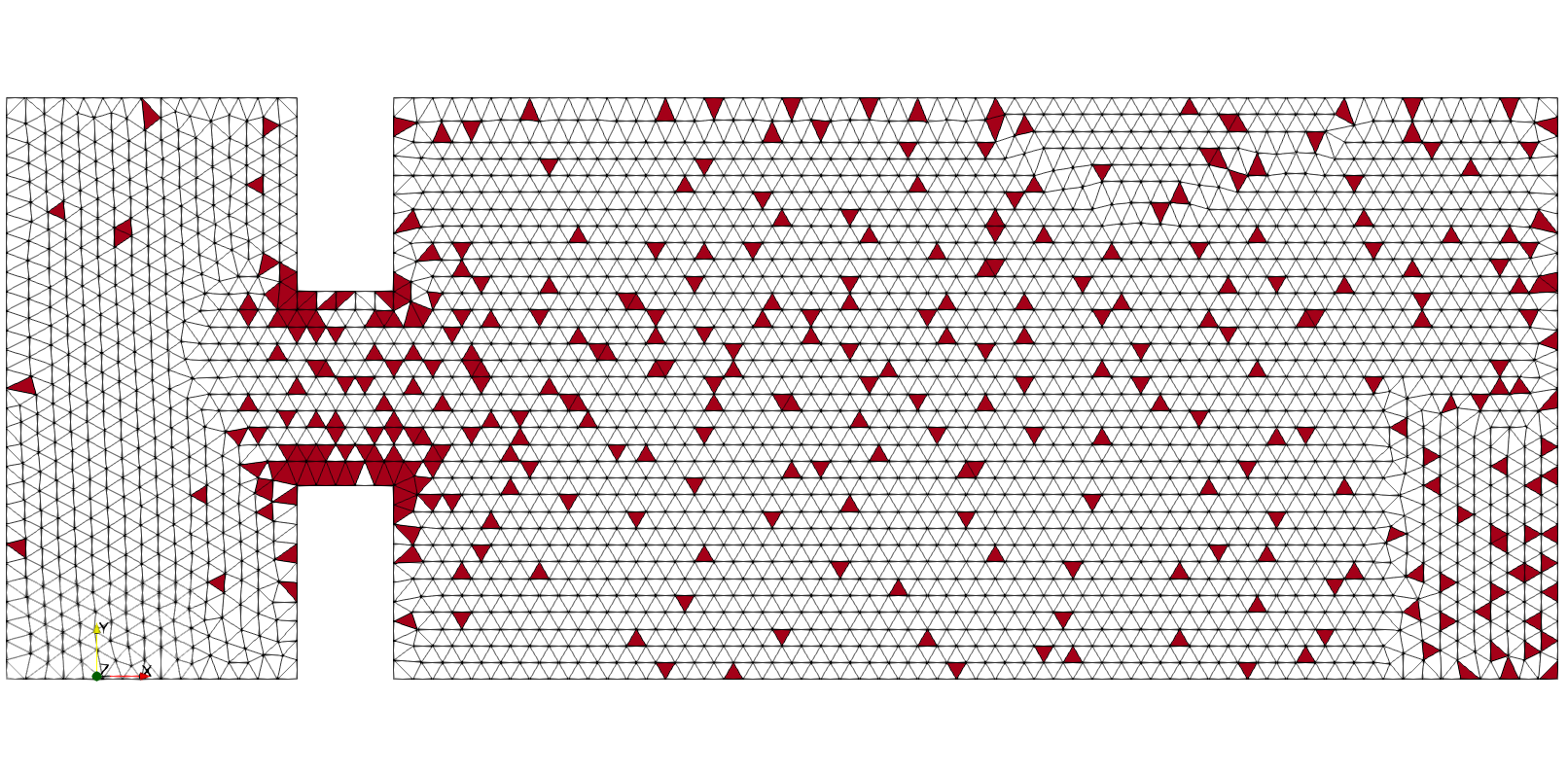
(b) $\epsilon_{\text{\tiny SOL}}=1e-3,\epsilon_{\text{\tiny RES}}=1e-4,$

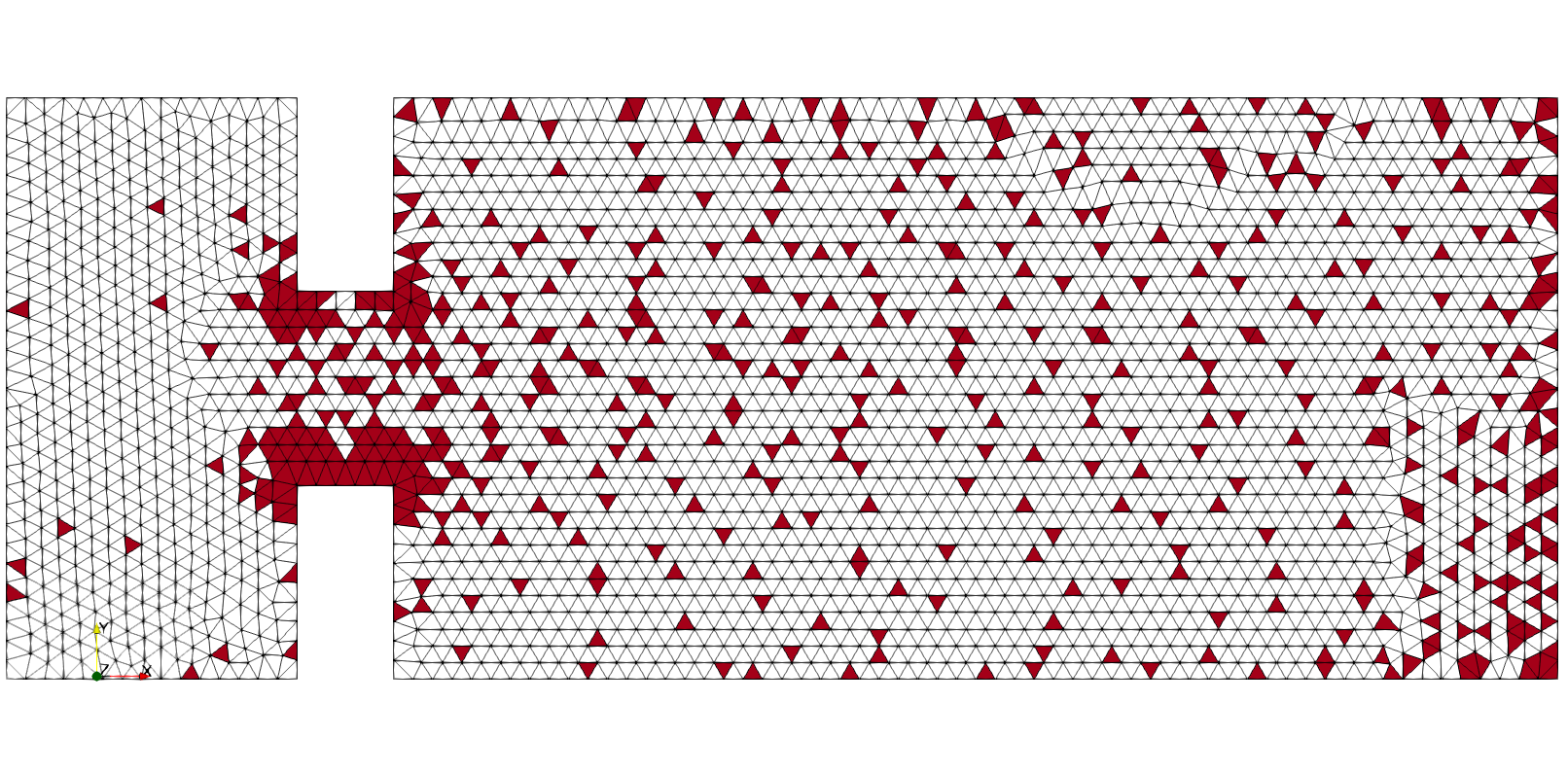
(c) $\epsilon_{\text{\tiny SOL}}=1e-3,\epsilon_{\text{\tiny RES}}=1e-5,$

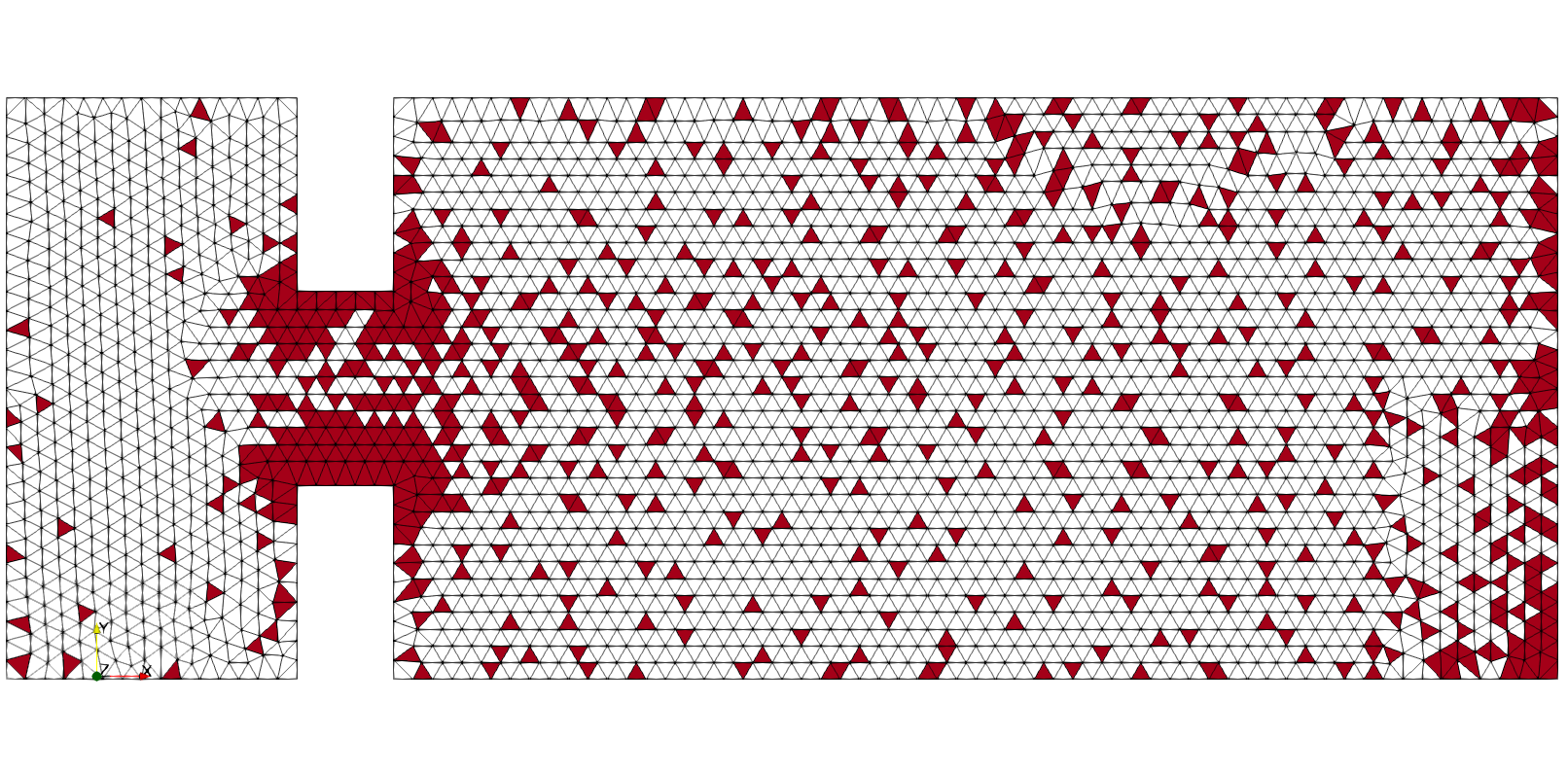
(d) $\epsilon_{\text{\tiny SOL}}=1e-3,\epsilon_{\text{\tiny RES}}=1e-6,$

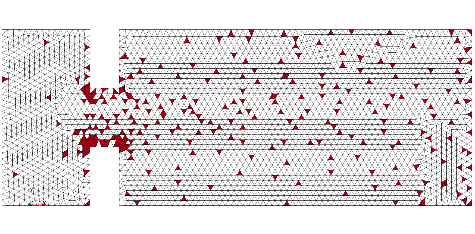
(e) $\epsilon_{\text{\tiny SOL}}=1e-4,\epsilon_{\text{\tiny RES}}=1e-3,$

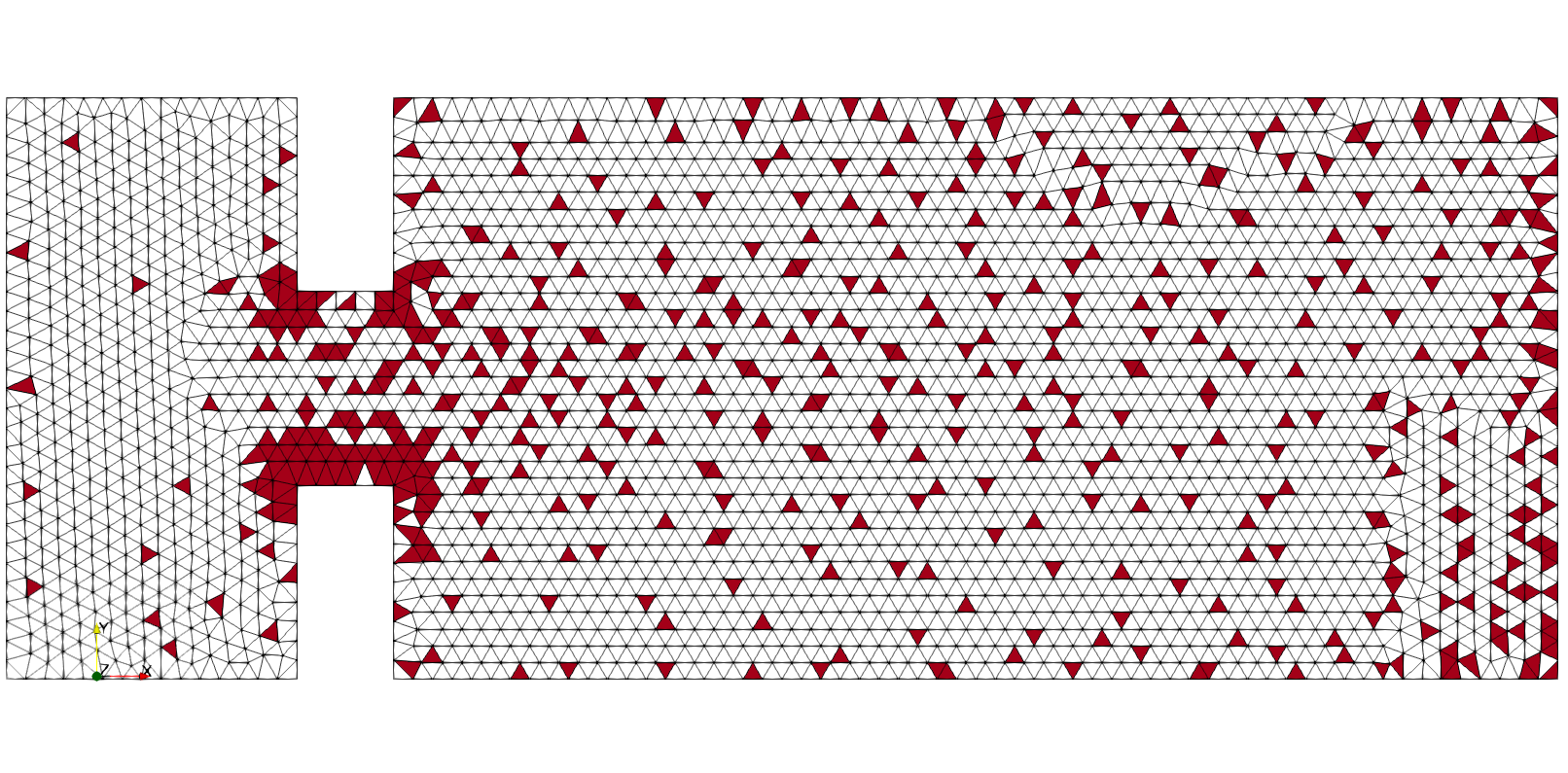
(f) $\epsilon_{\text{\tiny SOL}}=1e-4,\epsilon_{\text{\tiny RES}}=1e-4,$

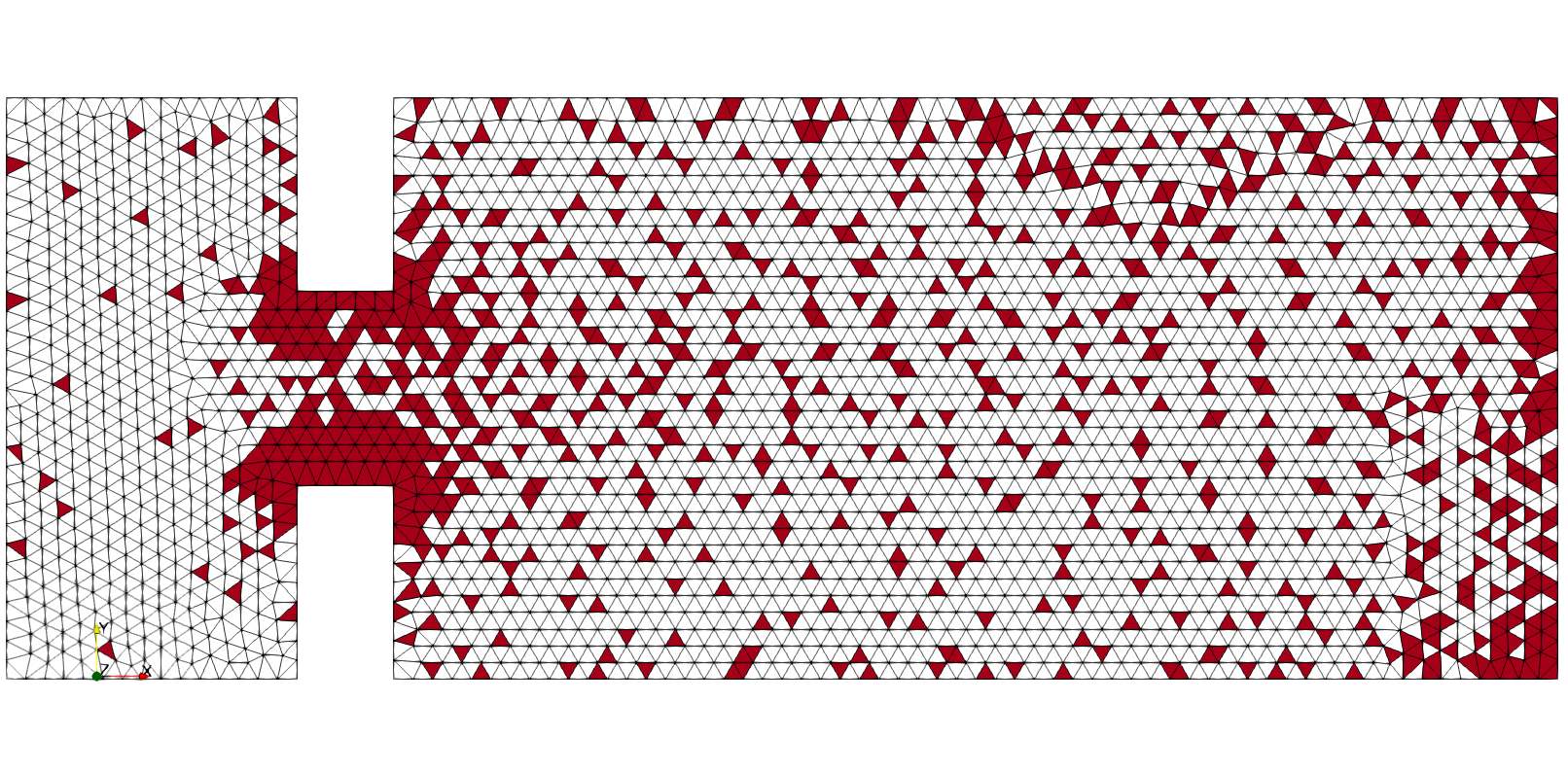
(g) $\epsilon_{\text{\tiny SOL}}=1e-4,\epsilon_{\text{\tiny RES}}=1e-5,$

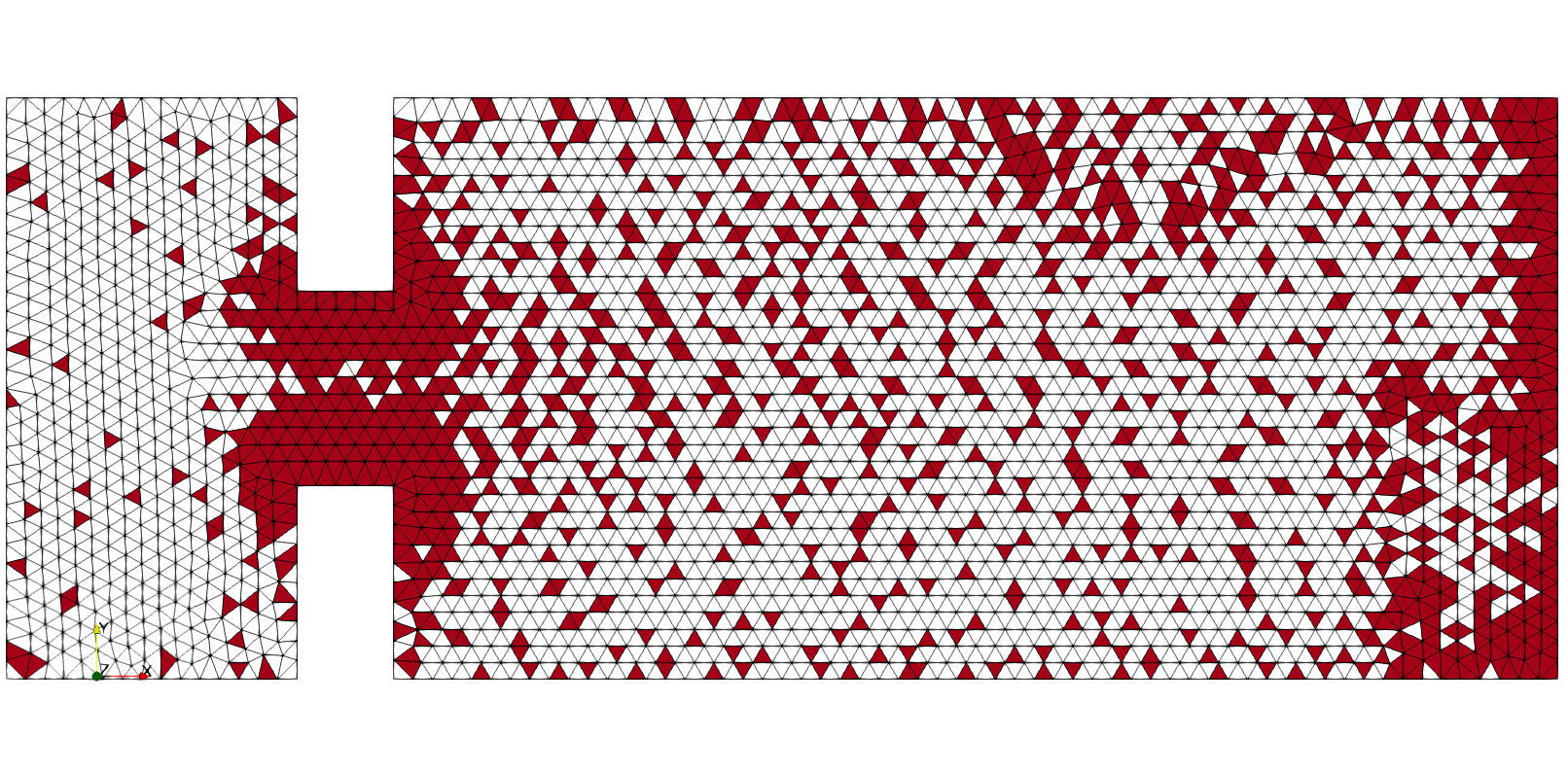
(h) $\epsilon_{\text{\tiny SOL}}=1e-4,\epsilon_{\text{\tiny RES}}=1e-6,$

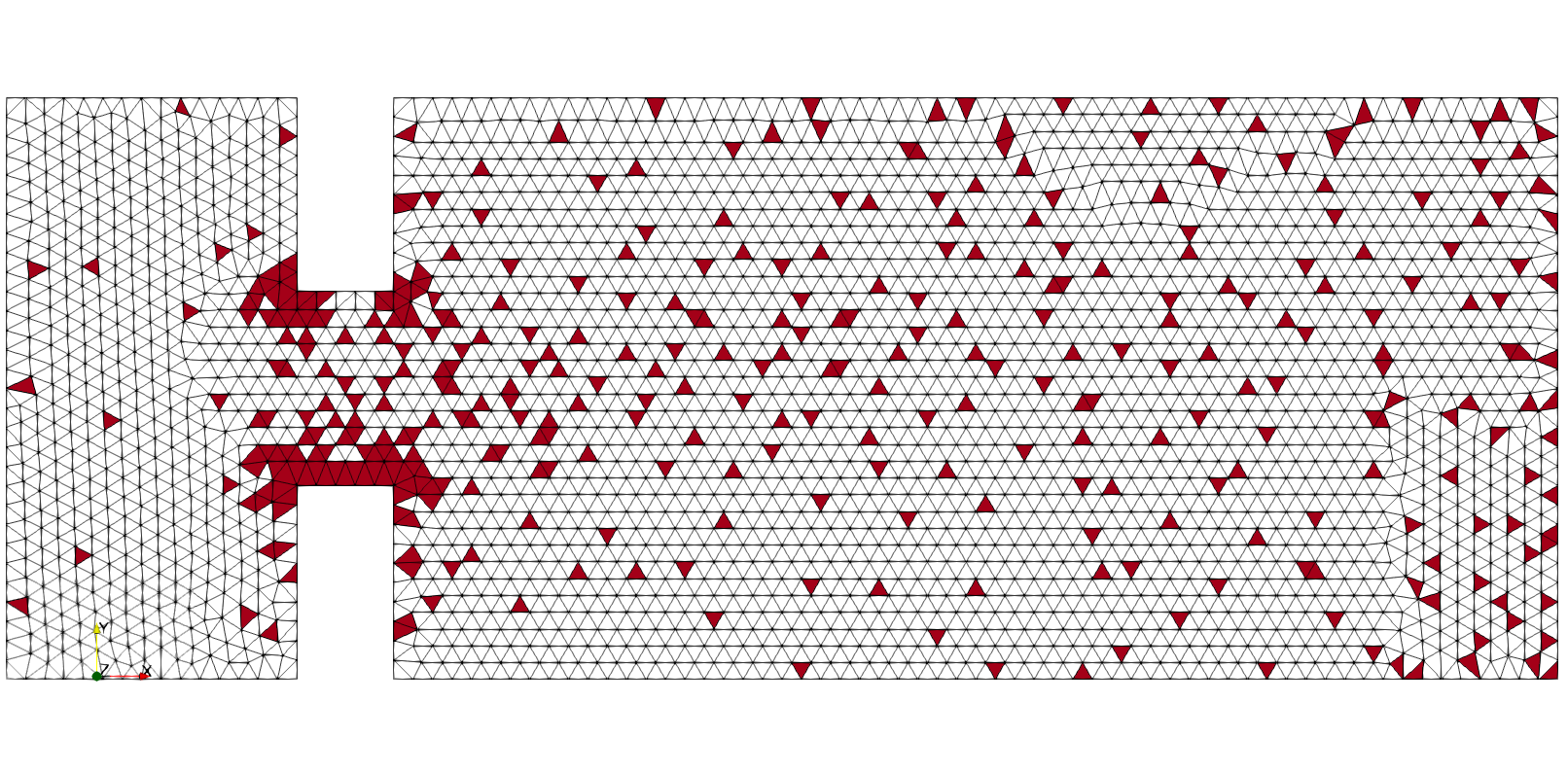
(i) $\epsilon_{\text{\tiny SOL}}=1e-5,\epsilon_{\text{\tiny RES}}=1e-3,$

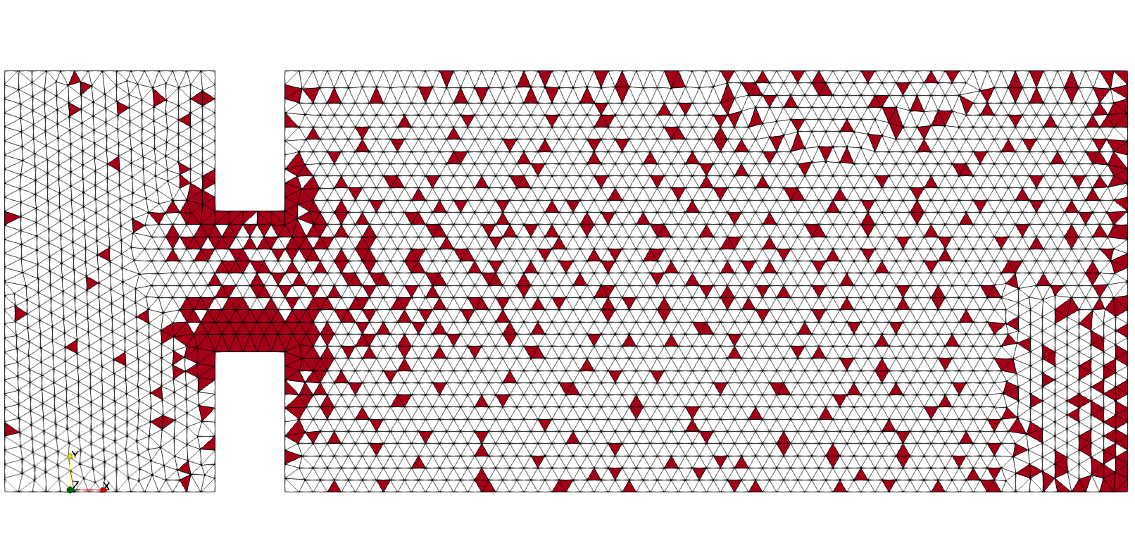
(j) $\epsilon_{\text{\tiny SOL}}=1e-5,\epsilon_{\text{\tiny RES}}=1e-4,$

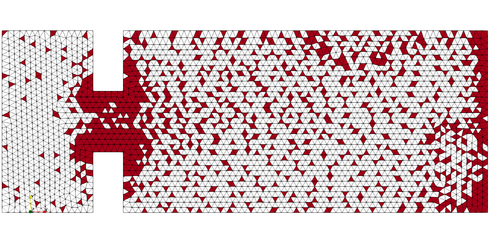
(k) $\epsilon_{\text{\tiny SOL}}=1e-5,\epsilon_{\text{\tiny RES}}=1e-5,$

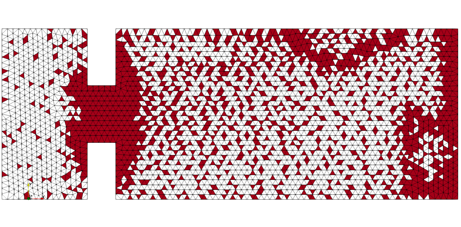
(l) $\epsilon_{\text{\tiny SOL}}=1e-5,\epsilon_{\text{\tiny RES}}=1e-6,$

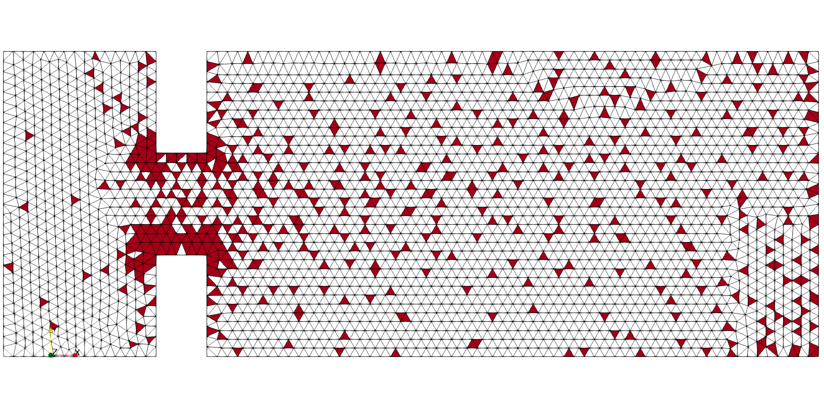
(m) $\epsilon_{\text{\tiny SOL}}=1e-6,\epsilon_{\text{\tiny RES}}=1e-3,$

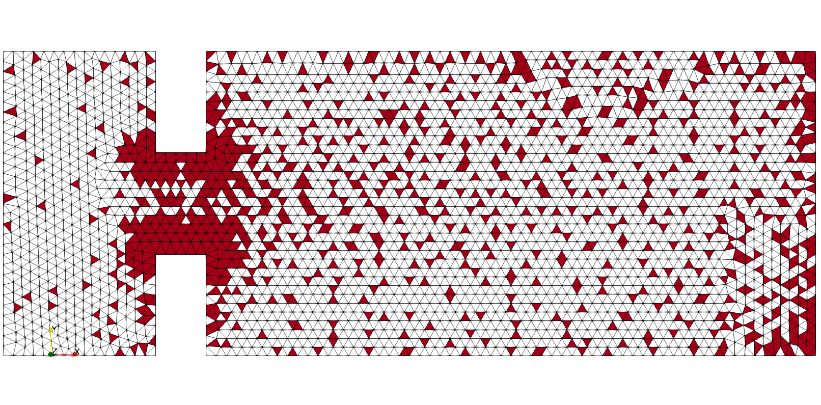
(n) $\epsilon_{\text{\tiny SOL}}=1e-6,\epsilon_{\text{\tiny RES}}=1e-4,$

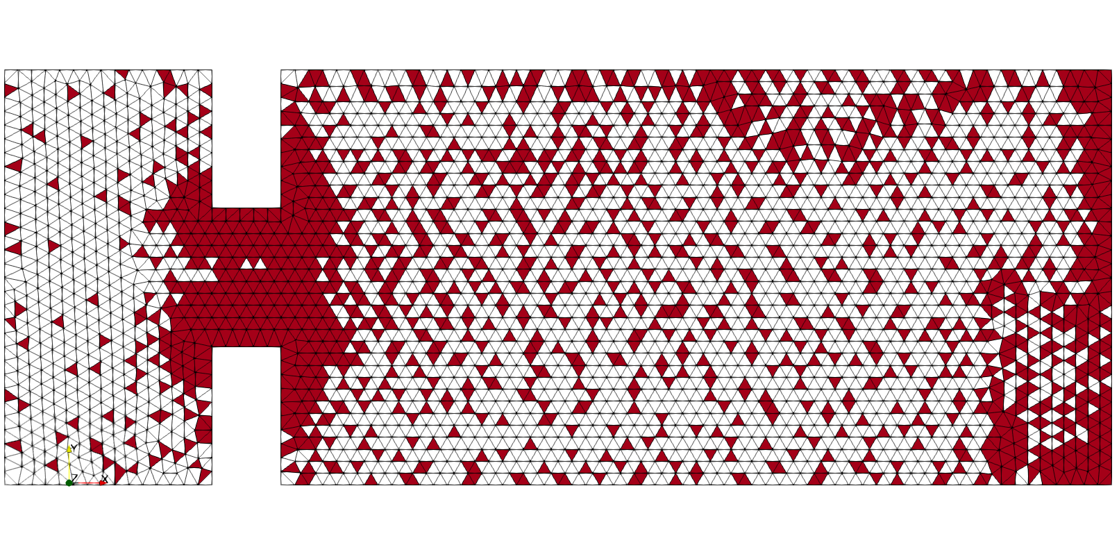
(o) $\epsilon_{\text{\tiny SOL}}=1e-6,\epsilon_{\text{\tiny RES}}=1e-5,$

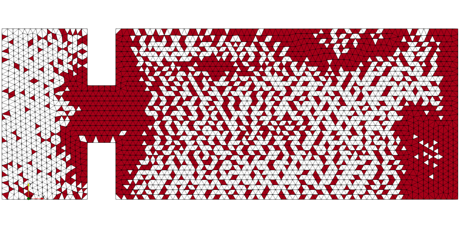
(p) $\epsilon_{\text{\tiny SOL}}=1e-6,\epsilon_{\text{\tiny RES}}=1e-6,$

Figure 20: Hyper-reduced elements selected for $\boldsymbol{\varphi}_{\text{\tiny FFD+RBF}}$

4.3.2 Hysteresis ROM vs HROM training trajectory

The hyper-reduced order models (HROMs) were utilised to reconstruct the training trajectories for both geometries. Fig. 21 and 22 depict the phase space reconstruction of the velocity at the probe points. In these plots, the ground truth is represented by the corresponding ROM solution, and the HROM solution serves as an approximation to the ROM. Any attempts to improve the HROM should result in convergence towards the ROM solution.

In the case of the affine mapping shown in Fig. 21, the simulations using the HROM constructed with a truncation tolerance of $\epsilon_{\text{\tiny RES}}=1e-3$ are not presented. These simulations consistently became unstable, yielding no useful data. Therefore, the largest truncation tolerance for the residual that is considered for the affine mapping is $\epsilon_{\text{\tiny RES}}=1e-4$. However, it can still be observed that the HROM simulation with this tolerance is deficient, as it exhibits visible differences from the ROM solution and still presents instabilities (see Figures 21(a), 21(d), 21(d)).

On the other hand, the phase space reconstruction of the training trajectory for the FFD+RBF mapping can be observed in Fig. 22. For this mapping, all four values of the truncation tolerance for the residual result in HROMs that produce stable solutions. However, it is noteworthy that using a larger value of $\epsilon_{\text{\tiny RES}}$ (e.g., Figures 24(a), 24(b), 24(c)) causes the solution to follow the opposite stable branch of the bifurcation. Only in Fig. 24(c), do all four studied values of $\epsilon_{\text{\tiny RES}}$ yield HROMs that follow the same bifurcation branch as the corresponding ROM.

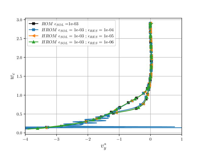
(a) ROM $1e-3$ vs HROM

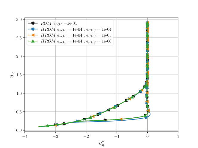
(b) ROM $1e-4$ vs HROM

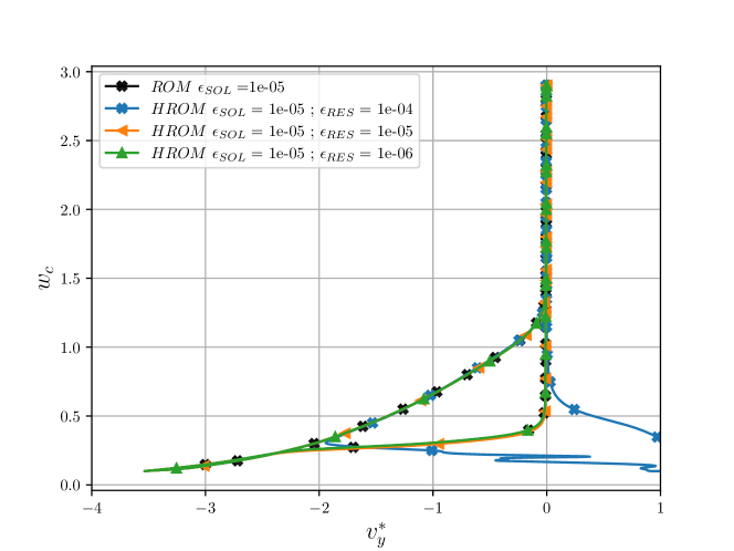
(c) ROM $1e-5$ vs HROM

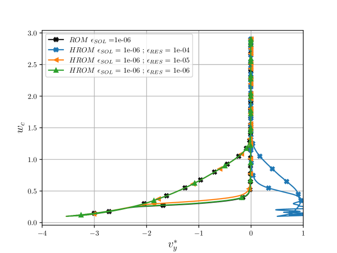
(d) ROM $1e-6$ vs HROM

Figure 21: ROM vs HROM hysteresis for training trajectory $\varphi_{\text{\tiny AFFINE}}$

(a) ROM $1e-3$ vs HROM

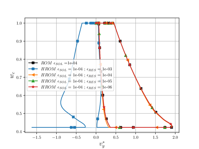
(b) ROM $1e-4$ vs HROM

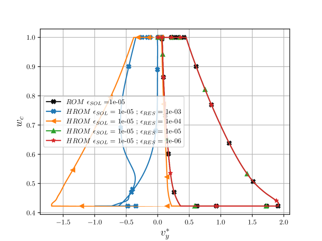
(c) ROM $1e-5$ vs HROM

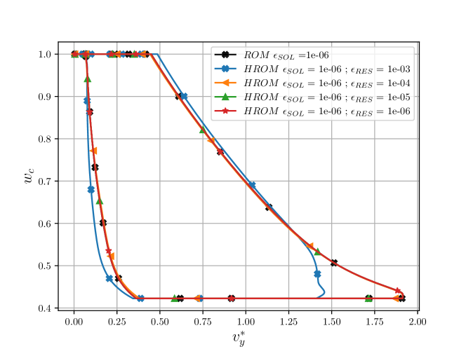
(d) ROM $1e-6$ vs HROM

Figure 22: ROM vs HROM hysteresis for training trajectory $\varphi_{\text{ \tiny FFD+RBF}}$

4.3.3 Hysteresis ROM vs HROM testing trajectory

Moving on to the reconstruction of the testing trajectory, we examine the results for both mappings. Figures 23 and 24 illustrate the ROM (taken as the ground truth) compared to the HROMs constructed using different truncation tolerances.

In the case of the affine mapping, where the FOM solution for the testing trajectory shows the jet attaching to the upper wall (Fig. 18(a)), all of the HROMs in Fig. 23 follow their respective ROMs, which means they take the opposite branch compared to the FOM. Furthermore, the HROMs with a tolerance of $\epsilon_{\text{\tiny RES}}=1e-3$ were unstable, similar to what was observed in the training trajectory.

In Fig. 24, the solutions for all combinations of truncation tolerances remain stable for the FFD+RBF mapping. However, the HROM with a truncation tolerance of $\epsilon_{\text{\tiny RES}}=1e-3$ produces solutions that deviate considerably from their corresponding ROMs. Specifically, in Fig. 24(d), the HROM with $\epsilon_{\text{\tiny RES}}=1e-3$ actually chooses the opposite branch of the bifurcation. It is important to recall that for the testing trajectory, the FOM consistently chose the lower branch (Fig. 18(b)).

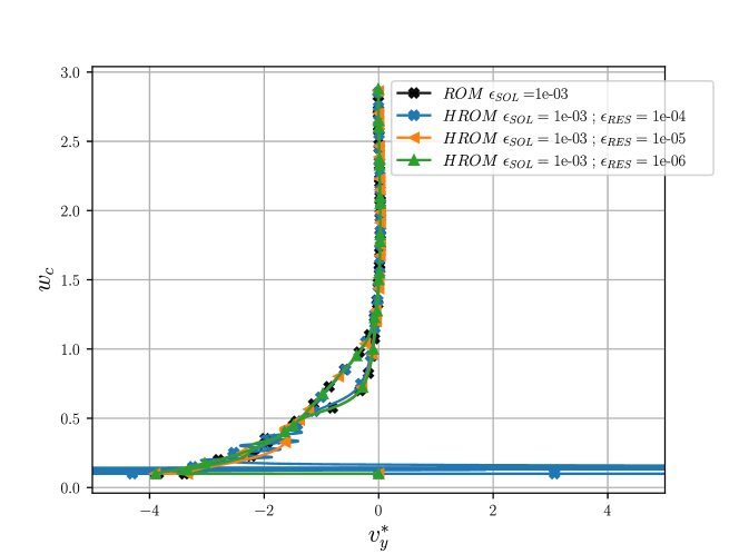
(a) ROM $1e-3$ vs HROM

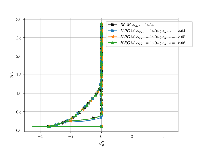
(b) ROM $1e-4$ vs HROM

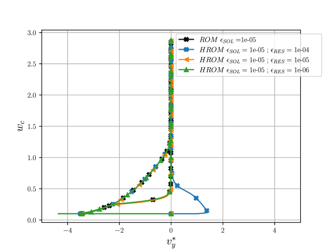
(c) ROM $1e-5$ vs HROM

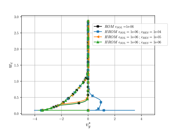
(d) ROM $1e-6$ vs HROM

Figure 23: ROM vs HROM hysteresis for testing trajectory $\varphi_{\text{\tiny AFFINE}}$

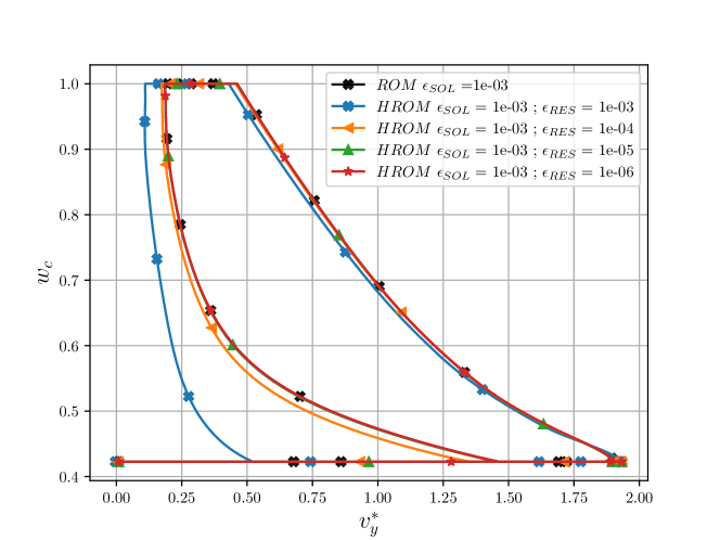
(a) ROM $1e-3$ vs HROM

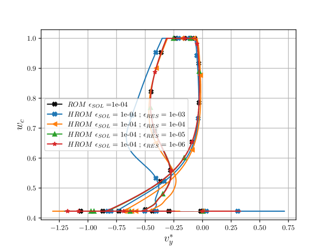
(b) ROM $1e-4$ vs HROM

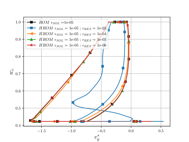
(c) ROM $1e-5$ vs HROM

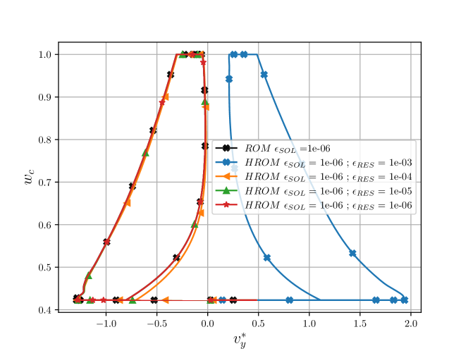
(d) ROM $1e-6$ vs HROM

Figure 24: ROM vs HROM hysteresis for testing trajectory $\varphi_{\text{\tiny FFD+RBF}}$

4.4 Error quantification

To quantitatively evaluate the results obtained for the different models, we define a percentage error operator as follows:

$$e: (\boldsymbol{a},\boldsymbol{b})\mapsto\frac{\left\lVert\boldsymbol{a}-\boldsymbol{b}\right\rVert}{\left\lVert\boldsymbol{a}\right\rVert}\cdot 100\ .$$ (53)

Here, $\boldsymbol{a}$ and $\boldsymbol{b}$ can be either matrices or column vectors. In our case, we will use this operator to compare the snapshots matrices of the solution fields for the FOM, ROM, and HROM, denoted respectively as $\boldsymbol{S}_{\text{\tiny FOM}}$, $\boldsymbol{S}_{\text{\tiny ROM}}$, and $\boldsymbol{S}_{\text{\tiny HROM}}$. We also quantify the error in the reconstruction of our quantity of interest (QoI) at the probe point $p^{*}$ (as shown in Figures 7 and 8), denoted as ${v^{*}_{y}}_{\text{\tiny FOM}}$, ${v^{*}_{y}}_{\text{\tiny ROM}}$, and ${v^{*}_{y}}_{\text{\tiny HROM}}$ for each of the considered models.

4.4.1 Error training trajectories

Table 2 and 3 provide a summary of the errors for the reconstruction of the training trajectories for both, the complete solution fields and the QoI.

For the affine mapping (Table 2), it can be observed that using only 11 modes for the ROM leads to a reconstruction error of 6% for the solution field. Increasing the number of modes does not significantly reduce the error, with the lowest error achieved at 1.8% already with 23 modes. In terms of the QoI error, it reaches its minimum value with 43 modes and increases slightly with 70 modes.

Regarding hyper-reduction, it is evident from the analysis in the previous sections and can be observed quantitatively here that using a tolerance of 1e-3 for the HROM selection algorithm results in unstable solutions. The minimum tolerance for the HROM element selection algorithm $\epsilon_{\text{\tiny RES}}$ appears to be 1e-4, and using 1e-5 yields better results.

$\epsilon_{SOL}$	# modes	$e\left({v^{*}_{y}}_{\text{\tiny FOM}},{v^{*}_{y}}_{\text{\tiny ROM}}\right)$	$e\left(\boldsymbol{S}_{\text{\tiny FOM}},\boldsymbol{S}_{\text{\tiny ROM}}\right)$	$\epsilon_{RES}$	# elems	$e\left({v^{*}_{y}}_{\text{\tiny ROM}},{v^{*}_{y}}_{\text{\tiny HROM}}\right)$	$e\left(\boldsymbol{S}_{\text{\tiny ROM}},\boldsymbol{S}_{\text{\tiny HROM}}\right)$
1e-3	11	38.41%	6.13%	1e-3	60	3620%	4323 %
				1e-4	143	101%	167 %
				1e-5	243	0.4%	0.32 %
				1e-6	388	0.03%	0.02 %
1e-4	23	4.07%	1.8%	1e-3	140	25188%	11647 %
				1e-4	354	11.54%	2.07%
				1e-5	621	0.36%	0.30%
				1e-6	930	0.1%	0.03%
1e-5	43	0.11%	1.8%	1e-3	233	1198%	2198%
				1e-4	555	111%	10%
				1e-5	1033	2.83%	0.12%
				1e-6	1652	0.45%	0.02%
1e-6	70	0.13%	1.8%	1e-3	348	685234%	3840455%
				1e-4	802	141%	3.13%
				1e-5	1442	10.68%	0.317%
				1e-6	2238	1.5%	0.05%

Table 2: Error summary for training trajectory for mapping $\boldsymbol{\varphi_{\text{\tiny AFFINE}}(\cdot,\mu)}$

The error results for the nonlinear geometric mapping are shown in (Table 3). In this case, the minimum number of modes is 19 and the maximum is 110. As in the case of the affine mapping, here the ROM employing 110 modes exhibits a slightly higher error in both the complete solution field and the QoI compared to the ROMs with 67 or 38 modes. Similar to the affine mapping, the tolerance of $\epsilon_{\text{\tiny RES}}=1e-3$ for the HROM element selection algorithm leads to comparatively large errors. However, in contrast to the affine mapping, all HROMs constructed with this tolerance remain stable.

In terms of the reconstruction of the complete solution field, it is observed that a minimum truncation tolerance of $\epsilon_{\text{\tiny RES}}=1e-4$ yields satisfactory results, with maximum errors ranging from 9.47% (for $\epsilon_{\text{\tiny SOL}}=1e-5$, $\epsilon_{\text{\tiny RES}}=1e-4$) to a minimum of 0.67% (for $\epsilon_{\text{\tiny SOL}}=1e-6$, $\epsilon_{\text{\tiny RES}}=1e-4$). However, when assessing the reconstruction of the QoI, it might be advisable to adopt a minimum tolerance of $\epsilon_{\text{\tiny RES}}=1e-5$ for HROM element selection, as it ensures errors below 1% in all cases studied.

$\epsilon_{SOL}$	# modes	$e\left({v^{*}_{y}}_{\text{\tiny FOM}},{v^{*}_{y}}_{\text{\tiny ROM}}\right)$	$e\left(\boldsymbol{S}_{\text{\tiny FOM}},\boldsymbol{S}_{\text{\tiny ROM}}\right)$	$\epsilon_{RES}$	# elems	$e\left({v^{*}_{y}}_{\text{\tiny ROM}},{v^{*}_{y}}_{\text{\tiny HROM}}\right)$	$e\left(\boldsymbol{S}_{\text{\tiny ROM}},\boldsymbol{S}_{\text{\tiny HROM}}\right)$
1e-3	19	15.9%	3.6%	1e-3	174	134.28%	12.35 %
				1e-4	351	10.50%	2.71 %
				1e-5	561	0.09%	0.02 %
				1e-6	819	0.001%	0.001 %
1e-4	38	0.44%	0.14%	1e-3	268	148.46 %	11.15 %
				1e-4	545	16.91 %	4.05 %
				1e-5	930	0.14 %	0.04 %
				1e-6	1412	0.001 %	0.001%
1e-5	67	0.16%	0.04%	1e-3	381	143.90 %	13.02 %
				1e-4	740	170.19 %	9.47 %
				1e-5	1232	0.26 %	0.05 %
				1e-6	1873	0.003 %	0.001 %
1e-6	110	0.6%	0.17%	1e-3	541	37.22 %	8.00 %
				1e-4	1018	2.20 %	0.67 %
				1e-5	1659	0.13 %	0.02 %
				1e-6	2428	0.01 %	0.003 %

Table 3: Error summary for training trajectory for mapping $\boldsymbol{\varphi_{\text{\tiny FFD+RBF}}(\cdot,\mu)}$

4.4.2 Error testing trajectories

The errors for the reconstruction of the testing trajectories, including the complete solution fields and the QoI, are summarized in Tables 4 and 5.

In Table 4, it is observed that the ROM using only 11 modes yields a 10% error in the reconstruction of the solution field compared to the FOM. As the number of modes increases, the error decreases, reaching a minimum of 8.99% with 70 modes. However, the errors in the QoI between the FOM and ROM remain above 145%. This is primarily due to the dominance of the opposite branch in the bifurcation diagram in the training trajectory, which differs from the branch induced by the FOM in this testing trajectory. The conclusions drawn from the training trajectory results regarding the tolerance parameter $\epsilon_{\text{\tiny RES}}$ for the HROM algorithm are equally applicable to the testing trajectory. A tolerance of $\epsilon_{\text{\tiny RES}}=1e-4$ yields potentially acceptable error values for the reconstruction of the solution field in the HROM compared to the corresponding ROM (except for the combination $\epsilon_{\text{\tiny SOL}}=1e-3$, $\epsilon_{\text{\tiny RES}}=1e-4$). However, for the reconstruction of the QoI, it is safer to adhere to tolerances of $\epsilon_{\text{\tiny RES}}=1e-5$ for the HROM selection algorithm.

$\epsilon_{SOL}$	# modes	$e\left({v^{*}_{y}}_{\text{\tiny FOM}},{v^{*}_{y}}_{\text{\tiny ROM}}\right)$	$e\left(\boldsymbol{S}_{\text{\tiny FOM}},\boldsymbol{S}_{\text{\tiny ROM}}\right)$	$\epsilon_{RES}$	# elems	$e\left({v^{*}_{y}}_{\text{\tiny ROM}},{v^{*}_{y}}_{\text{\tiny HROM}}\right)$	$e\left(\boldsymbol{S}_{\text{\tiny ROM}},\boldsymbol{S}_{\text{\tiny HROM}}\right)$
1e-3	11	147.42%	10.15%	1e-3	67	159423%	82877 %
				1e-4	165	1038%	732 %
				1e-5	284	4.17%	1.85 %
				1e-6	445	3.36%	0.28 %
1e-4	23	146.36%	9.29%	1e-3	141	195957%	627544 %
				1e-4	357	7.83%	1.54%
				1e-5	626	0.92%	0.77%
				1e-6	938	0.27%	0.07%
1e-5	43	145.93%	9.05%	1e-3	235	47853%	31811%
				1e-4	559	65.63%	3.68%
				1e-5	1042	2.03%	0.19%
				1e-6	1665	0.33%	0.07%
1e-6	70	145.77%	8.99%	1e-3	355	1428%	1214%
				1e-4	815	90.75%	1.86%
				1e-5	1464	6.72%	0.27%
				1e-6	2270	0.94%	0.02%

Table 4: Error summary for testing trajectory for mapping $\boldsymbol{\varphi_{\text{\tiny AFFINE}}(\cdot,\mu)}$

Table 5 presents the error in the reconstruction of the FOM solution field using a ROM, ranging from 11% with 19 modes to 4.4% with 110 modes. Moreover, for the same number of modes, the error in the QoI goes from 270% to 16.37%. This expected behavior can be attributed to the ROM’s ability to select the same branch in the bifurcation as the FOM for the testing trajectory, despite the training trajectory following the opposite branch.

Regarding the tolerance parameter $\epsilon_{\text{\tiny RES}}$ for the HROM element selection algorithm, it can be stated that it delivers acceptable errors in terms of the reconstruction of the solution field. However, these errors can still be significant when considering the QoI. For instance, the combination $\epsilon_{\text{\tiny SOL}}=1e-5$, $\epsilon_{\text{\tiny RES}}=1e-4$ results in an error of 11.3% for the ROM vs HROM comparison in the QoI.

$\epsilon_{SOL}$	# modes	$e\left({v^{*}_{y}}_{\text{\tiny FOM}},{v^{*}_{y}}_{\text{\tiny ROM}}\right)$	$e\left(\boldsymbol{S}_{\text{\tiny FOM}},\boldsymbol{S}_{\text{\tiny ROM}}\right)$	$\epsilon_{RES}$	# elems	$e\left({v^{*}_{y}}_{\text{\tiny ROM}},{v^{*}_{y}}_{\text{\tiny HROM}}\right)$	$e\left(\boldsymbol{S}_{\text{\tiny ROM}},\boldsymbol{S}_{\text{\tiny HROM}}\right)$
1e-3	19	270.1%	10.57%	1e-3	174	36.18%	7.60 %
				1e-4	351	4.20%	1.14 %
				1e-5	561	0.98%	0.27 %
				1e-6	819	0.31%	0.076 %
1e-4	38	46.03%	10.86%	1e-3	268	43.50 %	4.72 %
				1e-4	545	25.27 %	1.55 %
				1e-5	930	1.19 %	0.08 %
				1e-6	1412	0.79 %	0.05%
1e-5	67	42.56%	7.86%	1e-3	381	60.15 %	8.23 %
				1e-4	740	11.31 %	1.97 %
				1e-5	1232	1.97 %	0.33 %
				1e-6	1873	0.38 %	0.05 %
1e-6	110	16.37%	4.44%	1e-3	541	247.69 %	10.73 %
				1e-4	1018	3.46 %	2.77 %
				1e-5	1659	0.52 %	0.16 %
				1e-6	2428	0.172 %	0.07 %

Table 5: Error summary for testing trajectory for mapping $\boldsymbol{\varphi_{\text{\tiny FFD+RBF}}(\cdot,\mu)}$

4.5 Speedup

In order to quantify the speedup factor, a comparison was conducted between the ROM and the HROM in relation to the FOM. This analysis considered the time required for the construction and solution of the linear system of equations. The time necessary for visualising the complete solution field was not taken into account.

To evaluate the speedup factor, we introduced a speedup operator denoted as $s$, which operates as follows:

$$s: T_{\text{\tiny a }}\mapsto\frac{T_{\text{\tiny FOM }}}{T_{\text{\tiny a }}}\ ,$$ (54)

where $T_{\text{\tiny a }}$ represents the time required for either the ROM or the HROM, while $T_{\text{\tiny FOM }}$ corresponds to the time taken by the FOM. The output of this operator indicates the number of times the reduced order model is faster in comparison to the FOM.

The subsequent tables provide an overview of the speed-up factors obtained for both geometrical mappings, and all of the examined values of basis truncation $\epsilon_{\text{\tiny SOL}}$ and element selection truncation $\epsilon_{\text{\tiny RES}}$.

	ROM	HROM
$\epsilon_{\text{\tiny SOL}}$	$\epsilon_{\text{\tiny RES}}$
	-	1e-3	1e-4	1e-5	1e-6
1e-3	7 $\times$	276 $\times$	94 $\times$	30 $\times$	12 $\times$
1e-4	6 $\times$	154 $\times$	50 $\times$	13 $\times$	10 $\times$
1e-5	5.5 $\times$	126 $\times$	30 $\times$	9.8 $\times$	9 $\times$
1e-6	5 $\times$	84 $\times$	20 $\times$	9.1 $\times$	8 $\times$

Table 6: Speedup factor for mapping $\varphi_{\text{\tiny AFFINE}}$.

	ROM	HROM
$\epsilon_{\text{\tiny SOL}}$	$\epsilon_{\text{\tiny RES}}$
	-	1e-3	1e-4	1e-5	1e-6
1e-3	4 $\times$	57 $\times$	20 $\times$	7.5 $\times$	6 $\times$
1e-4	3.8 $\times$	28 $\times$	11 $\times$	7 $\times$	5.5 $\times$
1e-5	3.2 $\times$	21 $\times$	7.3 $\times$	5.7 $\times$	5.2 $\times$
1e-6	2.9 $\times$	15 $\times$	6.4 $\times$	5.5 $\times$	4.5 $\times$

Table 7: Speedup factor for mapping $\varphi_{\text{\tiny FFD+RBF}}$.

Based on the tabulated data, the speedup factors observed for the affine mapping surpass those of the FFD+RBF mapping. This discrepancy can be attributed to the fact that, at the point of maximum domain deformation, the model using the affine mapping necessitates a higher number of iterations by the solver, resulting in larger time savings.

When considering an admissible error threshold, employing the affine mapping with $\epsilon_{\text{\tiny SOL}}=1e-4$ and $\epsilon_{\text{\tiny RES}}=1e-4$ introduces a perceptual error ($e\left(\boldsymbol{S}{\text{\tiny FOM}},\boldsymbol{S}{\text{\tiny ROM}}\right)$) of approximately 2% in the training trajectory, while achieving a significant speedup of 50 times. However, this same error measure for the testing trajectory rises as high as 10%. By adopting more stringent tolerance values, such as $\epsilon_{\text{\tiny SOL}}=1e-5$ and $\epsilon_{\text{\tiny RES}}=1e-5$, the speedup is reduced to nearly 10 times, but the errors do not decrease substantially.

Conversely, in the case of the FFD+RBF mapping, utilising tolerances of $\epsilon_{\text{\tiny SOL}}=1e-4$ and $\epsilon_{\text{\tiny RES}}=1e-4$ yields speedup factors of 11 times, accompanied by errors $e\left(\boldsymbol{S}{\text{\tiny FOM}},\boldsymbol{S}{\text{\tiny ROM}}\right)$ of approximately 2% for the training trajectory and 10% for the testing trajectory.

Finally, we must report that we detected a significant increase in assembly time in our implementation as the number of POD modes increased. In scenarios where a large number of modes are involved, we deviated from the element-by-element approach outlined in Section 2.3 for assembling the system of equations. Instead, we adopted a “global” approach. This entailed assembling the sparse system matrix in a manner similar to the Full Order Model, followed by sparse-dense, and posterior dense-dense matrix product with the complete basis matrix $\boldsymbol{\Phi}$. We observed that the element-by-element formulations consistently outperformed the global approach for cases with truncation tolerances of $\epsilon_{\text{\tiny SOL}}\geq 1e-5$ and $\epsilon_{\text{\tiny RES}}\geq 1e-5$. The speedup factors reported in Tables 7 and 7 show the superior formulation between the two options.

5 Conclusions and Perspectives

In this paper, our focus was on investigating a general ROM framework for addressing time-dependent fluid dynamics problems with geometric parametrisations. This framework encompasses the utilisation of two powerful techniques: Proper Orthogonal Decomposition (POD) and Empirical Cubature Method (ECM) hyperreduction. By employing these techniques, we aimed to effectively capture the intricate fluid behavior inherent in the contraction-expansion channel geometry. While this geometry offers a relatively straightforward setting, it still presents complex fluid dynamics phenomena, such as a bifurcating solution known as Coanda effect.

By utilising ROMs and hyper-reduced order models (HROMs), we have successfully constructed accurate models capable of capturing both the training trajectories, which represent a specific deformation of the geometry over time, and the testing trajectories, which not only introduce different deformations of the domain, but also trigger the opposite branch of the bifurcation, compared to the training trajectory.

We have analysed the solution behavior in a phase-space, specifically focusing on a Quantity of Interest (QoI), which is the velocity in the y direction at a probe point. This QoI allows for the detection and characterisation of phenomena such as the Coanda effect and its hysteresis. By qualitatively assessing the outputs of the ROMs and HROMs in this phase-space plot, we gain insights into the performance of the models. Additionally, quantitative evaluations have been conducted to assess the accuracy of the complete solution field and the QoI.

As discussed in Sections 4.4 and 4.5, there is a trade-off between accuracy and computational speedup. The HROM models exhibit significant speedups, reaching 154$\times$ for the affine mapping and 57$\times$ for the nonlinear mapping, while still providing physically acceptable and bounded solutions. However, these models incur relatively large errors in reproducing the complete solution field and the QoI of the full order model, particularly for testing trajectories. Despite these errors, these models can still be useful in applications where the detection of the Coanda effect is crucial, even if the selected bifurcation branch is incorrect. For more accurate results, HROMs offering 50$\times$ and 11$\times$ speedups while maintaining low errors can be employed.

5.1 Future work

There are several promising avenues for further advancing this research.

Firstly, it is important to acknowledge that our study focused on a single parameter variation within a mesh comprising a relatively small number of elements, which was suitable for our academic objectives. However, in scenarios where higher resolution and increased accuracy are required, it becomes imperative to employ a larger number of elements in the base model. Additionally, an effective reduced order model should be trained by exploring a multidimensional parameter space. Addressing these considerations necessitates addressing certain challenges within the framework presented in this paper. Specifically, the launch and analysis of simulations, as well as the management of the generated matrices via singular value decomposition, become computationally demanding on a single machine.

As mentioned in Section 2.3.2, the size of the snapshots matrices increases with the number of elements and the number of POD modes. To alleviate this challenge, we are actively engaged in the development of parallelisation techniques for the entire workflow. This includes parallel simulation orchestration, efficient data management strategies, and the implementation of parallel algorithms for computing the singular value decomposition. These parallelisation efforts aim to significantly enhance the computational efficiency and scalability of the training process, enabling the exploration of larger parameter spaces and higher fidelity models.

Furthermore, simulations involving qualitatively distinct solutions, such as the ones demonstrated in this paper, often require a large number of modes to capture the intricate behavior of the solutions. To address this challenge, we are exploring alternative strategies. One approach involves utilising multiple piece-wise linear bases that effectively capture the specific behavior in the vicinity of a particular region in the parametric space, as demonstrated in [16, 19]. Additionally, we are investigating the utilisation of nonlinear manifolds, particularly quadratic approximations as proposed in [21, 3], to mitigate the requirement of a high number of modes. Lastly, we are actively exploring the application of autoencoder neural networks as a form of generic manifold Galerkin approximation [25, 38]. We anticipate that the results of these advancements will be reported in subsequent papers, expanding upon the findings presented in this study.

References

- [1] C. Allery, S. Guérin, A. Hamdouni, and A. Sakout. Experimental and numerical pod study of the coanda effect used to reduce self-sustained tones. Mechanics Research Communications, 31(1):105–120, 2004.
- [2] A. Ambrosetti and G. Prodi. A primer of nonlinear analysis. Number 34. Cambridge University Press, 1995.
- [3] J. Barnett and C. Farhat. Quadratic approximation manifold for mitigating the kolmogorov barrier in nonlinear projection-based model order reduction. Journal of Computational Physics, 464:111348, 2022.
- [4] A. Beckert and H. Wendland. Multivariate interpolation for fluid-structure-interaction problems using radial basis functions. Aerospace Science and Technology, 5(2):125–134, 2001.
- [5] S. Boyd, S. P. Boyd, and L. Vandenberghe. Convex optimization. Cambridge university press, 2004.
- [6] S. Chaturantabut and D. C. Sorensen. Nonlinear model reduction via discrete empirical interpolation. SIAM Journal on Scientific Computing, 32(5):2737–2764, 2010.
- [7] W. Cherdron, F. Durst, and J. H. Whitelaw. Asymmetric flows and instabilities in symmetric ducts with sudden expansions. Journal of Fluid Mechanics, 84(1):13–31, 1978.
- [8] J. Chung and G. Hulbert. A time integration algorithm for structural dynamics with improved numerical dissipation: the generalized- method. 1993.
- [9] R. Codina. Stabilized finite element approximation of transient incompressible flows using orthogonal subscales. Computer methods in applied mechanics and engineering, 191(39-40):4295–4321, 2002.
- [10] R. Codina, S. Badia, J. Baiges, and J. Principe. Variational multiscale methods in computational fluid dynamics. Encyclopedia of computational mechanics, pages 1–28, 2018.
- [11] J. Donea and A. Huerta. Finite element methods for flow problems. John Wiley & Sons, 2003.
- [12] C. Eckart and G. Young. The approximation of one matrix by another of lower rank. Psychometrika, 1(3):211–218, 1936.
- [13] V. M. Ferrándiz, P. Bucher, R. Zorrilla, R. Rossi, A. Cornejo, jcotela, M. A. Celigueta, J. Maria, tteschemacher, C. Roig, M. Masó, S. Warnakulasuriya, G. Casas, M. Núñez, P. Dadvand, S. Latorre, I. de Pouplana, J. I. González, F. Arrufat, riccardotosi, AFranci, A. Ghantasala, P. Wilson, dbaumgaertner, B. Chandra, A. Geiser, K. B. Sautter, I. Lopez, lluís, and J. Gárate. Kratosmultiphysics/kratos: Release 9.3, Feb. 2023.
- [14] J. Hernández. A multiscale method for periodic structures using domain decomposition and ecm-hyperreduction. Computer Methods in Applied Mechanics and Engineering, 368:113192, 2020.
- [15] J. A. Hernandez, M. A. Caicedo, and A. Ferrer. Dimensional hyper-reduction of nonlinear finite element models via empirical cubature. Computer methods in applied mechanics and engineering, 313:687–722, 2017.
- [16] M. Hess, A. Alla, A. Quaini, G. Rozza, and M. Gunzburger. A localized reduced-order modeling approach for pdes with bifurcating solutions. Computer Methods in Applied Mechanics and Engineering, 351:379–403, 2019.
- [17] M. W. Hess, A. Quaini, and G. Rozza. Reduced basis model order reduction for navier–stokes equations in domains with walls of varying curvature. International Journal of Computational Fluid Dynamics, 34(2):119–126, 2020.
- [18] M. W. Hess, A. Quaini, and G. Rozza. A spectral element reduced basis method for navier–stokes equations with geometric variations. Spectral and High Order Methods for Partial Differential Equations ICOSAHOM 2018, pages 561–571, 2020.
- [19] M. W. Hess, A. Quaini, and G. Rozza. Data-driven enhanced model reduction for bifurcating models in computational fluid dynamics. In ECCOMAS Congress 2022, 2022.
- [20] J. S. Hesthaven, G. Rozza, B. Stamm, et al. Certified reduced basis methods for parametrized partial differential equations, volume 590. Springer, 2016.
- [21] S. Jain, P. Tiso, J. B. Rutzmoser, and D. J. Rixen. A quadratic manifold for model order reduction of nonlinear structural dynamics. Computers & Structures, 188:80–94, 2017.
- [22] M. Khamlich, F. Pichi, and G. Rozza. Model order reduction for bifurcating phenomena in fluid-structure interaction problems. International Journal for Numerical Methods in Fluids, 94(10):1611–1640, 2022.
- [23] J. Lai and D. Lu. Effect of wall inclination on the mean flow and turbulence characteristics in a two-dimensional wall jet. International journal of heat and fluid flow, 17(4):377–385, 1996.
- [24] T. Lassila, A. Manzoni, A. Quarteroni, and G. Rozza. Model order reduction in fluid dynamics: challenges and perspectives. Reduced Order Methods for modeling and computational reduction, pages 235–273, 2014.
- [25] K. Lee and K. T. Carlberg. Model reduction of dynamical systems on nonlinear manifolds using deep convolutional autoencoders. Journal of Computational Physics, 404:108973, 2020.
- [26] M. Lombardi, N. Parolini, A. Quarteroni, and G. Rozza. Numerical simulation of sailing boats: dynamics, fsi, and shape optimization. In Variational Analysis and Aerospace Engineering: Mathematical Challenges for Aerospace Design: Contributions from a Workshop held at the School of Mathematics in Erice, Italy, pages 339–377. Springer, 2012.
- [27] A. Manzoni. Reduced models for optimal control, shape optimization and inverse problems in haemodynamics. Technical report, EPFL, 2012.
- [28] A. Melendo, A. Coll, M. Pasenau, E. Escolano, and A. Monros. www.gidhome.com, 2018. [Online; accessed Jun-2018].
- [29] J. Mizushima and Y. Shiotani. Transitions and instabilities of flow in a symmetric channel with a suddenly expanded and contracted part. Journal of Fluid Mechanics, 434:355–369, 2001.
- [30] B. Newman. The deflection of plane jets by adjacent boundaries-coanda effect. Boundary layer and flow control, 1961.
- [31] M. S. Oliveira, L. E. Rodd, G. H. McKinley, and M. A. Alves. Simulations of extensional flow in microrheometric devices. Microfluidics and nanofluidics, 5(6):809–826, 2008.
- [32] F. Pichi, F. Ballarin, G. Rozza, and J. S. Hesthaven. An artificial neural network approach to bifurcating phenomena in computational fluid dynamics. Computers & Fluids, 254:105813, 2023.
- [33] M. Pintore, F. Pichi, M. Hess, G. Rozza, and C. Canuto. Efficient computation of bifurcation diagrams with a deflated approach to reduced basis spectral element method. Advances in Computational Mathematics, 47(1):1–39, 2021.
- [34] G. Pitton, A. Quaini, and G. Rozza. Computational reduction strategies for the detection of steady bifurcations in incompressible fluid-dynamics: Applications to coanda effect in cardiology. Journal of Computational Physics, 344:534–557, 2017.
- [35] G. Pitton and G. Rozza. On the application of reduced basis methods to bifurcation problems in incompressible fluid dynamics. Journal of Scientific Computing, 73(1):157–177, 2017.
- [36] A. Quaini, R. Glowinski, and S. Čanić. Symmetry breaking and preliminary results about a hopf bifurcation for incompressible viscous flow in an expansion channel. International Journal of Computational Fluid Dynamics, 30(1):7–19, 2016.
- [37] A. Quarteroni and G. Rozza. Numerical solution of parametrized navier–stokes equations by reduced basis methods. Numerical Methods for Partial Differential Equations: An International Journal, 23(4):923–948, 2007.
- [38] F. Romor, G. Stabile, and G. Rozza. Non-linear manifold rom with convolutional autoencoders and reduced over-collocation method. arXiv preprint arXiv:2203.00360, 2022.
- [39] T. W. Sederberg and S. R. Parry. Free-form deformation of solid geometric models. In Proceedings of the 13th annual conference on Computer graphics and interactive techniques, pages 151–160, 1986.
- [40] L. Sirovich. Turbulence and the dynamics of coherent structures. i. coherent structures. Quarterly of applied mathematics, 45(3):561–571, 1987.
- [41] A. Skotnicka-Siepsiak. Pressure distribution on a flat plate in the context of the phenomenon of the coanda effect hysteresis. Scientific Reports, 12(1):1–13, 2022.
- [42] I. J. Sobey and P. G. Drazin. Bifurcations of two-dimensional channel flows. Journal of Fluid Mechanics, 171:263–287, 1986.
- [43] G. Stabile, F. Ballarin, G. Zuccarino, and G. Rozza. A reduced order variational multiscale approach for turbulent flows. Advances in Computational Mathematics, 45:2349–2368, 2019.
- [44] G. Stabile, M. Zancanaro, and G. Rozza. Efficient geometrical parametrization for finite-volume-based reduced order methods. International journal for numerical methods in engineering, 121(12):2655–2682, 2020.
- [45] M. Tezzele, N. Demo, A. Mola, and G. Rozza. PyGeM: Python Geometrical Morphing. Software Impacts, page 100047, 2020.
- [46] M. Tezzele, F. Salmoiraghi, A. Mola, and G. Rozza. Dimension reduction in heterogeneous parametric spaces with application to naval engineering shape design problems. Advanced Modeling and Simulation in Engineering Sciences, 5(1):1–19, 2018.
- [47] R. Wille and H. Fernholz. Report on the first european mechanics colloquium, on the coanda effect. Journal of Fluid Mechanics, 23(4):801–819, 1965.