Unique continuation for an elliptic interface problem using unfitted isoparametric finite elements

Abstract.

We study unique continuation over an interface using a stabilized unfitted finite element method tailored to the conditional stability of the problem. The interface is approximated using an isoparametric transformation of the background mesh and the corresponding geometrical error is included in our error analysis. To counter possible destabilizing effects caused by non-conformity of the discretization and cope with the interface conditions, we introduce adapted regularization terms. This allows to derive error estimates based on conditional stability. Numerical experiments suggest that the presence of an interface seems to be of minor importance for the continuation of the solution beyond the data domain. On the other hand, certain convexity properties of the geometry are crucial as has already been observed for many other problems without interfaces.

1. Introduction

1.1. Motivation

Recently, there has been an increasing interest in the development of numerical methods for unique continuation problems, see e.g. [10, 11, 4, 17, 7, 35, 21]. These methods are based on so called conditional stability estimates which represent a quantitative form of the unique continuation property for solutions of certain partial differential equations (PDEs). In addition, many physical applications involve interfaces over which material parameters can exhibit jump discontinuities, e.g. in seismic wave propagation. Despite the practical relevance of these problems, numerical methods for unique continuation involving interfaces seem to be unavailable in the literature.

On the other hand, the development of numerical methods, e.g. finite elements methods (FEMs), for well-posed problems involving interfaces is well advanced. So called unfitted FEMs are very appealing to treat these problems, see e.g. [27, 44, 34, 6, 42, 31, 8, 43, 19], since they allow the use of simple meshes which are independent of the possibly complex geometry of the interface. However, the analysis and implementation of unfitted FEMs imposes some challenges (stability of variational formulations, usually only an implicit description of the geometry is available, …) which are poorly understood in the context of ill-posed problems. In this paper, we make some progress in this direction by developing an unfitted FEM for a unique continuation problem involving an interface.

1.2. The problem setting

We define the problem setting as sketched in Figure 1. Let $\Omega\subset\mathbb{R}^{d},d\in\{2,3\}$, be a bounded, connected and open set split by a smooth interface $\Gamma$ into two connected components $\Omega_{1}$ and $\Omega_{2}$ such that $\Gamma=\partial\Omega_{1}$ and $\Omega=\Omega_{1}\cup\Gamma\cup\Omega_{2}$. Given the functions $u_{i}$ on $\Omega_{i}$, we identify $u$ on $\Omega_{1}\cup\Omega_{2}$ with the pair $(u_{1},u_{2})$.

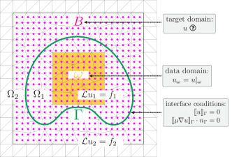
Figure 1. Sketch of geometry and data for unique continuation over an interface.

We consider the elliptic interface problem

$$\mathcal{L}u=f \text{ in }\Omega_{1}\cup\Omega_{2},$$ (1)

$$\llbracket u\rrbracket_{\Gamma}=0 \text{ on }\Gamma,$$ (2)

$$\llbracket\mu\nabla u\rrbracket_{\Gamma}\cdot n_{\Gamma}=0 \text{ on }\Gamma,$$ (3)

with $\mathcal{L}u:=-\nabla\cdot(\mu\nabla u)-\rho u$ for a quantity $\mu$ that is discontinuous across $\Gamma$ and constant on each $\Omega_{i}$ with $\mu_{i}:=\mu|_{\Omega_{i}}>0$. Similarly, $\rho$ is assumed to be piecewise constant such that $\rho_{i}:=\rho|_{\Omega_{i}}\in\mathbb{R}$. The jump over the interface $\Gamma$ is defined for $v=(v_{1},v_{2})\in H^{1}(\Omega_{1}\cup\Omega_{2})$ by $\llbracket v\rrbracket_{\Gamma}:=v_{1}-v_{2}$ and analogously for vector-valued functions. We fix the unit normal vector $n_{\Gamma}$ of $\Gamma$ to point from $\Omega_{1}$ into $\Omega_{2}$.

Note that no boundary data on $\partial\Omega$ is assumed to be given, which renders this problem ill-posed. To recover a weak form of stability, we will assume that measurements

$$u_{\omega}=u|_{\omega}$$ (4)

of a solution of (1)-(3) in a subset $\omega\subset\Omega$ are available. More precisely, we assume that $\omega$ is compactly contained in either $\Omega_{1}$ or $\Omega_{2}$. The objective is then to extend the solution from $\omega$ into a larger set $B\subset\Omega$ across the interface. From [20, Theorem 1.1], see Appendix A for details, we obtain that the following conditional stability estimate of Hölder-type holds. Let $\omega\subset B\subset\Omega$ such that $B\setminus\omega$ does not touch the boundary of $\Omega$ and $\omega$ is contained either in $\Omega_{1}$ or $\Omega_{2}$. Then for $u\in H^{1}(\Omega)$ we have

$$\left\lVert u\right\rVert_{B}\leqslant C\left(\left\lVert u\right\rVert_{\omega}+\left\lVert\mathcal{L}u\right\rVert_{H^{-1}(\Omega)}\right)^{\tau}\left(\left\lVert u\right\rVert_{\Omega}+\left\lVert\mathcal{L}u\right\rVert_{H^{-1}(\Omega)}\right)^{1-\tau}.$$ (5)

Here we introduced for $M\subset\mathbb{R}^{d}$ and $u,v\in L^{2}(M)$ the notation

$$(u,v)_{M}:=\int\limits_{M}uv\;\mathrm{d}x,\qquad\left\lVert v\right\rVert_{M}:=\sqrt{(v,v)_{M}}.$$

1.3. Content and structure of the article

In this article we propose a stabilized unfitted FEM for the numerical solution of (1)-(4). To cope with the fact that the problem merely enjoys conditional stability, see Corollary 1.2, we use the stabilization framework introduced in [5], which has been applied successfully to several different problems, see e.g. [11, 12, 13, 15, 7], using geometrically fitted discretizations. It turns out that some additional stabilization terms on the interface are necessary to allow for the use of an unfitted discretization.

Unfitted methods are usually based on an implicit description of the geometry, e.g. by levelset functions. Robust and accurate numerical integration on implicitly defined domains is challenging, which renders achieving high-order geometric accuracy with unfitted methods a difficult endeavor. Here, we adopt an approach developed in [28, 31, 32] based on an isoparametric mapping of the background mesh. In this framework the exact interface $\Gamma$ is represented numerically by an interface $\Gamma_{h}$ such that $\operatorname{dist}(\Gamma,\Gamma_{h})\leqslant Ch^{q+1}$ holds for a parameter $q\in\mathbb{N}$ which controls the geometric accuracy and a constant $C>0$ independent of the mesh width $h$. In contrast to well-posed problems, we find that the geometric error (stemming from $\Gamma\neq\Gamma_{h}$) exerts an additional destabilizing effect which has to be countered by a suitable regularization term.

As our main result (see Theorem 4.5) we show that the following error estimate for the extension of the solution given on the data domain $\omega$ to the target domain $B$ holds:

$$\left\lVert u-u_{h}\circ\Phi_{h}^{-1}\right\rVert_{B}\leqslant Ch^{\tau q}\left(\left\lVert u\right\rVert_{q}+h^{-q}\delta\right).$$

Here, $u_{h}$ is the numerical solution in an unfitted finite element space of order $p\geqslant q\geqslant 1$ and $\Phi_{h}$ is a continuous and piecewise smooth transformation mapping the exact to the approximate geometry. The term $\delta$ represent a data perturbation, $\tau\in(0,1)$ is the Hölder exponent from Corollary 1.2 and $\left\lVert u\right\rVert_{q}$ some Sobolev norm of the exact solution. Comparing our result with [11, 12, 13, 15], we conclude that (granted suitable stabilization is added) unfitted methods allow to solve unique continuation problems as good as their fitted counterparts.

We summarize the three main contributions of this article:

• We solve a unique conutinuation problem which involves an interface.

• We use an unfitted method to discretize an ill-posed problem and provide a fairly complete error analysis complemented by numerical experiments.

• In particular, our analysis allows arbitrary polynomial orders and includes geometric errors based on the technique from [28, 31, 32].

The remainder of this article is structured as follows. In Section 2 we explain how the geometry is resolved using the isoparametric mapping technique from [28, 31]. Some additional results for this technique are derived in this article which may be of independent interest. For example, we derive useful relations between derivates on the exact and approximate interface and show how the isoparametric mapping can be combined with a Galerkin-least squares stabilization. These results could be of interest in various setting, e.g. for convection-dominated problems, fluid problems involving interfaces or coupled bulk-surface problems. In Section 3 an unfitted isoparametric FEM for the problem (1)-(4) is introduced whose numerical analysis is carried out in Section 4. Numerical experiments are presented in Section 5. We conclude in Section 6.

2. Resolving the interface by an isoparametric mapping

This section deals with the geometrical approximation of the interface. In Subsection 2.1-2.3 three different levels of geometric accuracy will be introduced. We start in Subsection 2.1 with the exact geometry, proceed in Subsection 2.2 with the simplest approximation by a piecewise linear reference configuration and finish in Subsection 2.3 with the higher-order accurate approach from [28, 31] based on an isoparametric mapping. In Subsection 2.4 and Subsection 2.5 the basic properties of this mapping are recalled and some further extensions are derived. Please note that we have outsourced the proofs of this section into Appendix B.

2.1. The exact geometry

It is very common in unfitted FEMs to assume that the interface can be described by a smooth levelset function $\phi$ such that $\Gamma:=\{x\in\Omega\mid\phi(x)=0\}$. The corresponding subdomains are then given by $\Omega_{1}:=\{\phi<0\}$ and $\Omega_{2}:=\{\phi>0\}$. We introduce operators for restricting to these subdomains as follows:

$$(R_{1}u)(x):=\left\{\begin{array}[]{cc}u(x)&x\in\Omega_{1},\\ 0&\text{ else, }\end{array}\right.\quad(R_{2}u)(x):=\left\{\begin{array}[]{cc}u(x)&x\in\Omega_{2},\\ 0&\text{ else. }\end{array}\right.$$ (6)

Conversely, we need to be able to extend a function defined merely on a subdomain smoothly to all of $\Omega$. To this end, we utilize that our smoothness assumption on the interface guarantees, see [41, Theorem 5, Chapter VI], the existence of a linear and continuous Sobolev extension operator

$$\mathcal{E}_{i}:W^{m,p}(\Omega_{i})\rightarrow W^{m,p}(\mathbb{R}^{d}),\quad\text{such that }\mathcal{E}_{i}|_{\Omega_{i}}=\mathrm{id},\;i=1,2,$$ (7)

available for all $m\in\mathbb{N}_{0}$ and $1\leqslant p\leqslant\infty$. Here, $W^{m,p}(\Omega_{i})$ are the standard Sobolev spaces which we denote by $H^{m}(\Omega_{i})$ when $p=2$ as usual. For $u\in W^{m,p}(\Omega_{1}\cup\Omega_{2})$ it is convenient to use the notation $\mathcal{E}u=(\mathcal{E}u_{1},\mathcal{E}u_{2})$.
Further, we will have to consider derivatives along and normal to the interface. As in the introduction let $n_{\Gamma}$ be the unit normal vector on $\Gamma$ pointing from $\Omega_{1}$ into $\Omega_{2}$. Based on $n_{\Gamma}$ we define the tangential projection $P_{\Gamma}:=I-n_{\Gamma}(n_{\Gamma})^{T}$ and surface gradient $\nabla_{\Gamma}:=P_{\Gamma}\nabla$.

2.2. The piecewise linear reference geometry

Let us first introduce a quasi-uniform and simplicial triangulation $\mathcal{T}_{h}$ of $\Omega$, which is assumed to be independent of $\Gamma$. We use the notation $\lesssim$ (and $\sim$ for $\lesssim$ and $\gtrsim$) to denote that an inequality holds with a constant independent of $h$ and how the interface intersects the triangulation $\mathcal{T}_{h}$. In this work we would like to focus attention on how the geometrical resolution of the interface influences the reconstruction. To eliminate other sources of geometrical errors we assume (as in the sketch given in Figure 1):

Assumption 1.

Let $\Omega$ and $\omega$ be polygonal domains which are exactly fitted by $\mathcal{T}_{h}$.

We denote by $V_{h,p}$ the standard $H^{1}$-conforming finite element space on $\mathcal{T}_{h}$ based on piecewise polynomials of order $p$ and set $V_{h,p}^{0}:=\{v_{h}\in V_{h,p}\mid v_{h}|_{\partial\Omega}=0\}$. Let $\hat{\phi}$ be the piecewise linear nodal interpolation of $\phi$ into $V_{h,1}$. Based on $\hat{\phi}$ we define the piecewise linear reference interface $\Gamma^{\text{lin}}:=\{x\in\Omega\mid\hat{\phi}(x)=0\}$, respectively the subdomains $\Omega^{\text{lin}}_{1}:=\{\hat{\phi}<0\}$ and $\Omega^{\text{lin}}_{2}:=\{\hat{\phi}>0\}$. An illustration of some of these geometrical quantities is given in Figure 2. Further, the intersection of an element with $\Gamma^{\text{lin}}$ is denoted by $\Gamma_{T}:=T\cap\Gamma^{\text{lin}}$. We combine all the elements cut by the interface into the set $\mathcal{T}^{\Gamma}:=\{T\in\mathcal{T}_{h}\mid\Gamma_{T}\neq\emptyset\}$ with corresponding domain $\Omega^{\Gamma}:=\{x\in T\mid T\in\mathcal{T}^{\Gamma}\}$.
We now turn our attention to the elements in the bulk. Let $T_{i}:=T\cap\Omega^{\text{lin}}_{i}$ denote the portion of the element in $\Omega^{\text{lin}}_{i}$ and define the active mesh $\mathcal{T}_{h}^{i}:=\{T\in\mathcal{T}_{h}\mid T_{i}\neq\emptyset\}$ and corresponding active domain $\Omega^{+}_{i}:=\{x\in T:T\in\mathcal{T}_{h}^{i}\}$. As for the physical domains we define corresponding restriction operators which give rise to the so called Cut-FEM space:

$$(R_{i}^{+}u)(x):=\left\{\begin{array}[]{cc}u(x)&x\in\Omega_{i}^{+},\\ 0&\text{ else, }\end{array}\right.\qquad V_{h,p}^{\Gamma}:=R_{1}^{+}V_{h,p}\oplus R_{2}^{+}V_{h,p}.$$ (8)

Elements $v_{h}\in V_{h,p}^{\Gamma}$ have the form $v_{h}=(v_{h,1},v_{h,2})$ with $v_{h,i}\in R_{i}^{+}V_{h,p}$. Note that the introduced description of the geometry is only second order accurate, i.e. $\operatorname{dist}(\Gamma,\Gamma_{h})\lesssim\mathcal{O}(h^{2})$, which limits the overall accuracy of derived numerical method unless some form of correction is applied, see e.g. [9, 3].

2.3. The isoparametric mapping

The higher-order description of the geometry from [28, 31] is based on an interpolant $\phi_{h}\in V_{h,q},q\in\mathbb{N}$ of the levelset function in a higher-order finite element space. To circumvent that for $q\geqslant 2$ the geometry description given by $\phi_{h}$ is only implicit, a mapping $\Theta_{h}\in[V_{h,q}]^{d}$ is constructed based on $\phi_{h}$ and $\hat{\phi}$ which maps the piecewise linear reference geometry to a higher order accurate approximation of the exact geometry, i.e. we have

$$\hat{\phi}\approx\phi_{h}\circ\Theta_{h}\;\text{and for }\Gamma_{h}:=\Theta_{h}(\Gamma^{\text{lin}})\text{ it holds: }\operatorname{dist}(\Gamma,\Gamma_{h})\lesssim\mathcal{O}(h^{q+1}).$$

This means that $\Gamma_{h}$ defined as the image of the piecewise linear reference interface under the mapping $\Theta_{h}$ and $\Omega_{i,h}:=\Theta_{h}(\Omega^{\text{lin}}_{i})$ approximate the exact interface and subdomains with order $\mathcal{O}(h^{q+1})$ and thanks to

$$\int\limits_{\Omega_{i,h}}{f\;dx}=\int\limits_{\Omega^{\text{lin}}_{i}}{f\circ\Theta_{h}\left\lvert\det{\left(D\Theta_{h}\right)}\right\rvert\;dy}$$ (9)

it suffices to compute integrals on the piecewise linear reference configuration which is well-understood, see e.g. [6, Section 5] for details. We also define $\Omega_{i,h}^{+}:=\Theta_{h}(\Omega_{i}^{+})$.
For the analysis (not the implementation) we will need another mapping $\Psi$ which maps the piecewise linear reference geometry back to the exact geometry, in particular  $\Psi(\Gamma^{\text{lin}})=\Gamma$ holds. The transformation $\Theta_{h}$ is invertible for sufficiently small $h$ (see [31, Section 3.5]) and we can define $\Phi_{h}=\Psi\circ\Theta_{h}^{-1}$, which then fulfills $\Phi_{h}(\Gamma_{h})=\Gamma$ and has the smoothness property $\Phi_{h}\in[C(\Omega)]^{d}\cap[C^{q+1}(\Theta_{h}(\mathcal{T}_{h}))]^{d}$, see [32]. For a detailed description on how the mappings $\Theta_{h}$ and $\Psi$ are constructed we refer to [31, Section 3]. Here, we only recall the fact that both mappings are small perturbations of the identity whose action is localized in the vicinity of the interface. In particular, as $\omega$ is compactly contained in one of the subdomains it follows that for sufficiently small $h$ it holds

$$\Phi_{h}|_{\omega}=\mathrm{id}.$$ (10)

Let us close this subsection by defining some geometrical quantities on the discrete interface $\Gamma_{h}$. Let $n_{\Gamma_{h}}$ denote the unit normal vector on $\Gamma_{h}$. We also define the discrete tangential projection $P_{\Gamma_{h}}:=I-n_{\Gamma_{h}}(n_{\Gamma_{h}})^{T}$ and surface gradient $\nabla_{\Gamma_{h}}:=P_{\Gamma_{h}}\nabla$.

2.4. Basic properties of the mappings

As noted above, the mesh transformation is essentially a small perturbation of the identity. A quantitative version of this statement has been given in [31, Lemma 5.5] which is recalled below. Let $\underline{A}:=D\Phi_{h}$. The following holds

$$\left\lVert\Theta_{h}-\Psi\right\rVert_{\infty,\Omega}+h\left\lVert D(\Theta_{h}-\Psi)\right\rVert_{\infty,\Omega} \lesssim h^{q+1},$$ (11)

$$\left\lVert\Phi_{h}-\mathrm{id}\right\rVert_{\infty,\Omega}+h\left\lVert\underline{A}-I\right\rVert_{\infty,\Omega} \lesssim h^{q+1}.$$ (12)

Here, $\left\lVert\cdot\right\rVert_{\infty,M}$ denotes the $L^{\infty}$-norm on $M\subset\mathbb{R}^{d}$. From the proof of [31, Lemma 5.10] we also recall the following estimates:

$$\left\lVert\underline{A}^{-1}-I\right\rVert_{\infty,\Omega}\lesssim h^{q},\quad\left\lVert\det(\underline{A})-1\right\rVert_{\infty,\Omega}\lesssim h^{q},\quad\left\lVert C_{\Phi_{h}}\right\rVert_{\infty,\Omega}\lesssim h^{q},$$ (13)

where $C_{\Phi_{h}}:=(\underline{A}^{T}\underline{A})^{-1}\det(\underline{A})-I$. Notice also that this implies $\left\lVert\det(A^{-1})\right\rVert_{\infty,\Omega}\lesssim 1$ for $h$ sufficiently small. We will additionally require bounds for higher derivatives of $\Phi_{h}$ which were stated in [31, Remark 5.6] without proof. [Higher order bounds for $\Phi_{h}$] For $l=2,\cdots,q+1$ it holds that

1. $\max_{T\in\mathcal{T}_{h}}\left\lVert D^{l}(\Psi-\Theta_{h})\right\rVert_{\infty,T}\lesssim h^{q+1-l}$.

2. $\max_{T\in\mathcal{T}_{h}}\left\lVert D^{l}(\Phi_{h}-\mathrm{id})\right\rVert_{\infty,\Theta_{h}(T)}=\max_{T\in\mathcal{T}_{h}}\left\lVert D^{l}\Phi_{h}\right\rVert_{\infty,\Theta_{h}(T)}\lesssim h^{q+1-l}.$

Proof.

Given in Appendix B like the other proofs of this section. ∎

In the analysis we will frequently have to transform between exact and discrete interface. To this end, it is important to understand how the respective normal vectors and associated projections are related. We recall from [31, eq. (A.20)] that the transformation $\Phi_{h}$ induces the relations

$$n_{\Gamma}\circ\Phi_{h}=\frac{\underline{A}^{-T}n_{\Gamma_{h}}}{\left\lVert\underline{A}^{-T}n_{\Gamma_{h}}\right\rVert_{2}},\quad n_{\Gamma_{h}}\circ\Phi_{h}^{-1}=\frac{\underline{A}^{T}n_{\Gamma}}{\left\lVert\underline{A}^{T}n_{\Gamma}\right\rVert_{2}}.$$ (14)

Using these relations and (12) it is easy to show: [Normal and tangential projection] For $h$ sufficiently small the following estimates hold uniformly on $\Gamma$, respectively $\Gamma_{h}$.

1. On $\Gamma$ we have

   $$\left\lVert\underline{A}^{T}n_{\Gamma}\right\rVert_{2}\gtrsim 1\text{ and }\left\lvert\left\lVert\underline{A}^{T}n_{\Gamma}\right\rVert_{2}-1\right\rvert\lesssim h^{q},$$

   and on $\Gamma_{h}$:

   $$\left\lVert\underline{A}^{-T}n_{\Gamma_{h}}\right\rVert_{2}\gtrsim 1\text{ and }\left\lvert\left\lVert\underline{A}^{-T}n_{\Gamma_{h}}\right\rVert_{2}-1\right\rvert\lesssim h^{q}.$$

2. The perturbation of the exact normal vector is bounded by:

   $$\left\lVert n_{\Gamma}-n_{\Gamma_{h}}\circ\Phi_{h}^{-1}\right\rVert_{2}\lesssim h^{q}\text{ on }\Gamma,\quad\left\lVert n_{\Gamma}\circ\Phi_{h}-n_{\Gamma_{h}}\right\rVert_{2}\lesssim h^{q}\text{ on }\Gamma_{h}.$$

3. As a result, the tangential projections satisfy:

   $$\left\lVert P_{\Gamma_{h}}\circ\Phi_{h}^{-1}-P_{\Gamma}\right\rVert_{2}\lesssim h^{q},\text{ on }\Gamma,\quad\left\lVert P_{\Gamma}\circ\Phi_{h}-P_{\Gamma_{h}}\right\rVert_{2}\lesssim h^{q},\text{ on }\Gamma_{h}.$$

We remark that results similar to Lemma 14 already appear in [26, Lemma 3.3] and [33, Lemma 17].

2.5. Geometry errors for mapped functions

Since $\Phi_{h}$ maps the discrete to the exact geometry, precomposition with this map allows to pull back functions defined on the exact geometry to the discrete geometry and vice versa. The following two lemmas discuss how various norms of these functions are related. [norm equivalence] Let $\tilde{v}:=v\circ\Phi_{h}$ for $v\in H^{1}(\Omega_{i})\cap H^{2}(\Psi(\mathcal{T}_{h}^{i}))$. Then it holds that

1. $\left\lVert\tilde{v}\right\rVert_{\Omega_{i,h}}\sim\left\lVert v\right\rVert_{\Omega_{i}}$ and $\left\lVert\nabla\tilde{v}\right\rVert_{\Omega_{i,h}}\sim\left\lVert\nabla v\right\rVert_{\Omega_{i}}$.

2. For the second derivatives we have for $\nu,\mu\in\{1,\ldots,d\}$:

   $$\sum\limits_{T\in\mathcal{T}_{h}^{i}}\int\limits_{\Theta_{h}(T)}\left\lvert\partial_{y_{\nu}}\partial_{y_{\mu}}\tilde{v}\right\rvert^{2}\;\mathrm{d}y\lesssim\sum\limits_{\left\lvert\alpha\right\rvert\leqslant 2}\sum\limits_{T\in\mathcal{T}_{h}^{i}}\int\limits_{\Psi(T)}\left\lvert D_{x}^{\alpha}v\right\rvert^{2}\;\mathrm{d}x.$$

While the norms involving the full gradients on $\Gamma$ and $\Gamma_{h}$ are equivalent, the corresponding statement for the normal and tangential derivatives only holds up to a geometrical error proportional to $h^{q}$. In view of Lemma 14 this has to be expected. [Derivatives at the interface] Let $\tilde{v}:=v\circ\Phi_{h}$ for $v\in H^{1}(\Gamma)$. Then

1. We have $\left\lVert v\right\rVert_{\Gamma}\sim\left\lVert\tilde{v}\right\rVert_{\Gamma_{h}}$ and $\left\lVert\nabla v\right\rVert_{\Gamma}\sim\left\lVert\nabla\tilde{v}\right\rVert_{\Gamma_{h}}$.

2. For the normal derivates:

   $$\left\lVert\nabla\tilde{v}\cdot n_{\Gamma_{h}}\right\rVert_{\Gamma_{h}}\lesssim h^{q}\left\lVert\nabla v\right\rVert_{\Gamma}+\left\lVert\nabla v\cdot n_{\Gamma}\right\rVert_{\Gamma},\quad\left\lVert\nabla v\cdot n_{\Gamma}\right\rVert_{\Gamma}\lesssim h^{q}\left\lVert\nabla\tilde{v}\right\rVert_{\Gamma_{h}}+\left\lVert\nabla\tilde{v}\cdot n_{\Gamma_{h}}\right\rVert_{\Gamma_{h}}.$$

3. And for tangential derivatives:

   $$\left\lVert\nabla_{\Gamma_{h}}\tilde{v}\right\rVert_{\Gamma_{h}}\lesssim h^{q}\left\lVert\nabla v\right\rVert_{\Gamma}+\left\lVert\nabla_{\Gamma}v\right\rVert_{\Gamma},\quad\left\lVert\nabla_{\Gamma}v\right\rVert_{\Gamma}\lesssim h^{q}\left\lVert\nabla\tilde{v}\right\rVert_{\Gamma_{h}}+\left\lVert\nabla_{\Gamma_{h}}\tilde{v}\right\rVert_{\Gamma_{h}}.\quad$$

Finally, we will have to quantify the extent to which a function $f\circ\Phi_{h}^{-1}(x)$ differs from $f(x)$ when compared at the same point $x$. Clearly, smoothness assumptions need to be imposed on $f$ if one wants to guarantee that the difference is small. We remark that part (a) and (b) of the following lemma have been used before in the literature, see e.g. [29, in proof of Lemma 12]. [Pullback] Let $M\subset\Omega$ and $U,V\subset\Omega$ be open sets that are sufficiently large to contain all line segments between points in $\Phi_{h}^{-1}(M)$ and $M$, respectively between $\Phi_{h}(M)$ and $M$.

1. For $f\in W^{1,\infty}(U)$ we have $\left\lVert f\circ\Phi_{h}^{-1}-f\right\rVert_{M}\lesssim h^{q+1}\sqrt{\left\lvert M\right\rvert}\left\lVert\nabla f\right\rVert_{\infty,U}$, where $\left\lvert M\right\rvert$ denotes the Lebesgue measure of $M$.

2. For $f\in W^{2,\infty}(U)$ we have

   $$\left\lVert\nabla(f\circ\Phi_{h}^{-1}-f)\right\rVert_{M}\lesssim h^{q+1}\sqrt{\left\lvert M\right\rvert}\left\lVert f\right\rVert_{W^{2,\infty}(U)}+h^{q}\left\lVert\nabla{f}\right\rVert_{M}.$$

3. For $M=\Theta_{h}(T)$ with $T\in\mathcal{T}_{h}$ and $f\in W^{3,\infty}(V)$ it holds that

   $$\left\lVert f\circ\Phi_{h}-f\right\rVert_{H^{2}(M)}\lesssim h^{q-1}\sqrt{\left\lvert M\right\rvert}\left\lVert f\right\rVert_{W^{3,\infty}(V)}.$$

4. Moreover, for $f\in H^{2}(\Psi(T))$ we have

   $$\left\lVert\partial_{x_{\nu}}\partial_{x_{\mu}}(f\circ\Phi_{h})\circ\Phi_{h}^{-1}-\partial_{x_{\nu}}\partial_{x_{\mu}}f\right\rVert_{\Psi(T)}\lesssim h^{q}\left\lVert f\right\rVert_{H^{2}(\Psi(T))}+h^{q-1}\left\lVert\nabla f\right\rVert_{\Psi(T)}.$$

3. Isoparametric unfitted FEM

In this section we introduce a stabilized FEM for the solution of (1)-(4). Based on the technique to resolve the interface discussed in Section 2 we start in Subsection 3.1 by introducing isoparametric FEM spaces. In Subsection 3.2 we define the actual discrete variational formulation, discuss stabilization terms and record some basic properties including stability and bounds on geometric errors. The final Subsection 3.3 deals with interpolation into unfitted isoparametric FEM spaces.

3.1. Isoparametric finite element spaces

Following [31] we define the following isoparametric FEM spaces: For $\clubsuit\in\{\Gamma,0\}$:

$$V_{h,\Theta}^{\clubsuit}:=\{v_{h}\circ\Theta_{h}^{-1}\mid v_{h}\in V_{h,p}^{\clubsuit}\},\quad V_{h,\Phi}^{\clubsuit}:=\{v_{h}\circ\Phi_{h}^{-1}\mid v_{h}\in V_{h,\Theta}^{\clubsuit}\},$$ (15)

$$V_{h,\Psi}^{\clubsuit}:=\{v_{h}\circ\Psi_{h}^{-1}\mid v_{h}\in V_{h,p}^{\clubsuit}\}.$$ (16)

Note that $V_{h,\Theta}^{\Gamma}$ is an isoparametric version of the Cut-Finite element space defined in (8), while $V_{h,\Theta}^{0}$ is based on a standard finite element space on the background mesh with homogeneous Dirichlet boundary conditions on $\partial\Omega$. Since the mappings $\Psi$ and $\Theta_{h}$ reduce to the identity away from the interface, it follows that functions in the transformed spaces vanish on $\partial\Omega$ as well.
Let us also note that some of the tools frequently used in the analysis involving the spaces $V_{h,p}^{\clubsuit}$ easily carry over to their curved counterparts. Indeed, as $w_{h}\in V_{h,\Theta}^{\clubsuit}$ is of the form $w_{h}=v_{h}\circ\Theta_{h}^{-1}$ with $v_{h}\in V_{h,p}^{\clubsuit}$ and we have from [31, Lemma 3.14] the relations

$$\left\lVert\nabla w_{h}\right\rVert_{\Theta_{h}(T)}\sim\left\lVert\nabla v_{h}\right\rVert_{T}\text{ and }\left\lVert w_{h}\right\rVert_{\Theta_{h}(T)}\sim\left\lVert v_{h}\right\rVert_{T}$$ (17)

we can transfer standard inverse inequalities from $v_{h}$ to $w_{h}$, e.g.

$$\left\lVert\nabla w_{h}\right\rVert_{\Theta_{h}(T)}\sim\left\lVert\nabla v_{h}\right\rVert_{T}\lesssim h^{-1}\left\lVert v_{h}\right\rVert_{T}\sim h^{-1}\left\lVert w_{h}\right\rVert_{\Theta_{h}(T)}.$$ (18)

Since $\left\lVert w_{h}\right\rVert_{\Theta_{h}(\Gamma_{T})}\sim\left\lVert v_{h}\right\rVert_{\Gamma_{T}}$, we also obtain in analogy to the case with piecewise linear geometry, see [27], that

$$\left\lVert w_{h}\right\rVert_{\Theta_{h}(\Gamma_{T})}^{2}\lesssim h^{-1}\left\lVert w_{h}\right\rVert_{\Theta_{h}(T)}^{2}+h^{1}\left\lVert\nabla w_{h}\right\rVert_{\Theta_{h}(T)}^{2}.$$ (19)

We remark that (17) and (19) are valid for general $w=v\circ\Theta_{h}^{-1}$ with $v\in H^{1}(T)$.

3.2. Stabilized method for unique continuation

Let us start by defining the bilinear forms usually employed for the unfitted discretization of problem (1)-(3) when homogeneous Dirichlet boundary conditions on $\partial\Omega$ are given. In the bulk we define

$$a(u,v):=\sum\limits_{i=1,2}(\mu_{i}\nabla u_{i},\nabla v_{i})_{\Omega_{i}}-(\rho_{i}u_{i},v_{i})_{\Omega_{i}},$$ (20)

and analogously on the discrete geometry

$$a_{h}(u,v):=\sum\limits_{i=1,2}(\mu_{i}\nabla u_{i},\nabla v_{i})_{\Omega_{i,h}}-(\rho_{i}u_{i},v_{i})_{\Omega_{i,h}}.$$ (21)

On the interface we define

$$N^{c}(u,v):=\int\limits_{\Gamma}\{\!\!\{-\mu\nabla v\}\!\!\}\cdot n_{\Gamma}\llbracket u\rrbracket\;\mathrm{d}S,\quad\{\!\!\{\mu\nabla v\}\!\!\}\cdot n_{\Gamma}:=\kappa_{1}\mu_{1}\nabla v_{1}\cdot n_{\Gamma}+\kappa_{2}\mu_{2}\nabla v_{2}\cdot n_{\Gamma}$$ (22)

for convex weights $\kappa_{1}+\kappa_{2}=1$ in the numerical flux. Note that $N^{c}(u,v)=0$ for the exact solution $u$ of (1)-(3) holds. On the discrete geometry we define $N^{c}_{h}$ analogously where the integration is now over $\Gamma_{h}$ and the exact normal is replaced by $n_{\Gamma_{h}}$. We combine bulk and interface terms into

$$A(u,v):=a(u,v)+N^{c}(u,v),\quad A_{h}(u,v):=a_{h}(u,v)+N_{h}^{c}(u,v).$$ (23)

Notice that $N_{h}^{c}(u,v)$ is the only term on the interface remaining in a standard unfitted Nitsche formulation [27] when $v$ is continuous across $\Gamma$.

Next we proceed to the definition of the linear forms. Let $f_{i}=\mathcal{L}u_{i}\in W^{1,\infty}(\Omega_{i})$ be the exact right hand side of (1). In applications exact data is usually not available. We merely have access to perturbed data

$$\tilde{f}_{i}:=f_{i}+\delta f_{i},\quad\delta f_{i}\in L^{2}(\Omega_{i}).$$

For implementation, we have to extend the data $\tilde{f}_{i}$ given on $\Omega_{i}$ to $\Omega_{i,h}$. To this end, we use the Sobolev extension operator from (7). Hence,

$$\mathcal{E}_{i}\tilde{f}_{i}=\mathcal{E}_{i}f_{i}+\mathcal{E}_{i}\delta f_{i}:=f_{i,h}+\delta f_{i,h}$$

is well defined on $\Omega_{1,h}\cup\Omega_{2,h}$. Note that

$$\left\lVert f_{i,h}\right\rVert_{W^{1,\infty}(\Omega_{i,h})}\lesssim\left\lVert f_{i}\right\rVert_{W^{1,\infty}(\Omega_{i})},\quad\left\lVert\delta f_{i,h}\right\rVert_{\Omega_{i,h}}\lesssim\left\lVert\delta f_{i}\right\rVert_{\Omega_{i}}$$

holds by continuity of the extension. We write $f_{h}:=(f_{1,h},f_{1,h})$ and the same for $\delta f_{h}$ and $\mathcal{E}\tilde{f}$. Then we define the linear forms

$$\ell(w):=(f,w)_{\Omega_{1}\cup\Omega_{2}},\;\ell_{h}(w_{h}):=(f_{h},w_{h})_{\Omega_{1,h}\cup\Omega_{2,h}},\;\tilde{\ell}_{h}(w_{h}):=(\mathcal{E}\tilde{f},w_{h})_{\Omega_{1,h}\cup\Omega_{2,h}}.$$

We proceed analogously for the data domain. Recall that $u_{\omega}:=u|_{\omega}$ for $u$ being the exact solution of (1)-(3). We assume perturbed data

$$\tilde{u}_{\omega}:=u_{\omega}+\delta u_{\omega},\quad\delta u_{\omega}\in L^{2}(\omega)$$

is given. The strength of the entire data perturbation is measured in the norm

$$\delta:=\left\lVert\delta u_{\omega}\right\rVert_{\omega}+\left\lVert\delta f\right\rVert_{\Omega_{1}\cup\Omega_{2}}.$$ (24)

To define a stable method for the unique continuation problem, we follow the approach introduced in [5]. The idea is to formulate the ill-posed problem as a discrete optimization problem consisting of a data fidelity term: $\left\lVert u_{h}-\tilde{u}_{\omega}\right\rVert_{\omega}$, a term to enforce the PDE constraint: $A_{h}(u_{h},z_{h})-\tilde{\ell}_{h}(z_{h})$, where $z_{h}$ represents a Lagrange multiplier, and suitable stabilization terms to guarantee unique solvability and incorporate a priori knowledge of the solution. The stabilized FEM is then obtained from the first order optimality condition. For brevity we will skip the described steps here, which can be found in the literature e.g. [5, 11, 12, 13, 15], and advance immediately to the discrete variational formulation given as follows. Find $(u_{h},z_{h})\in V_{h,\Theta}^{\Gamma}\times V_{h,\Theta}^{0}$ such that

$$B_{h}[(u_{h},z_{h}),(v_{h},w_{h})]=(\tilde{u}_{\omega},v_{h})_{\omega}+\tilde{\ell}_{h}(w_{h})+\sum\limits_{i=1,2}\sum\limits_{T\in\mathcal{T}_{h}^{i}}h^{2}(\mathcal{E}_{i}\tilde{f}_{i},\mathcal{L}v_{h,i})_{\Theta_{h}(T_{i})}$$

$$=(u_{\omega},v_{h})_{\omega}+\ell_{h}(w_{h})+\sum\limits_{i=1,2}\sum\limits_{T\in\mathcal{T}_{h}^{i}}h^{2}(f_{i,h},\mathcal{L}v_{h,i})_{\Theta_{h}(T_{i})}+g(v_{h},w_{h})$$ (25)

with

$$g(v_{h},w_{h}):=(\delta u_{\omega},v_{h})_{\omega}+(\delta f_{h},w_{h})_{\Omega_{1,h}\cup\Omega_{2,h}}+\sum\limits_{i=1,2}\sum\limits_{T\in\mathcal{T}_{h}^{i}}h^{2}(\delta f_{i,h},\mathcal{L}v_{h,i})_{\Theta_{h}(T_{i})},$$

$$B_{h}[(u_{h},z_{h}),(v_{h},w_{h})]=A_{h}(v_{h},z_{h})+s_{h}(u_{h},v_{h})+(u_{h},v_{h})_{\omega}$$

$$\phantom{B_{h}[(u_{h},z_{h}),(v_{h},w_{h})]}+A_{h}(u_{h},w_{h})-s_{h}^{\ast}(z_{h},w_{h}).$$ (26)

We remark that as $z_{h}$ is continuous across the interface, the variables $z_{h,i}$ which appear in the definition of $A_{h}(v_{h},z_{h})$ (see e.g. (21)) are simply the restriction of $z_{h}$ to the respective subdomains. It remains to define the primal $s_{h}(\cdot,\cdot)$ and dual $s_{h}^{\ast}(\cdot,\cdot)$ stabilization terms. We commence by introducing the constituents of the former. A fairly standard component of methods based on the framework in [5] are Galerkin-least squares:

$$J_{\mathrm{GLS}}\left(u_{h},v_{h}\right):=\sum\limits_{i=1,2}\sum\limits_{T\in\mathcal{T}_{h}^{i}}h^{2}(\mathcal{L}u_{h,i},\mathcal{L}v_{h,i})_{\Theta_{h}(T_{i})}$$

and continuous interior penalty terms:

$$J_{\mathrm{CIP}}\left(u_{h},v_{h}\right):=\sum\limits_{i=1,2}\sum\limits_{F\in\mathcal{F}^{i}}h\!\!\int\limits_{\Theta_{h}(F)}\!\!\mu_{i}\llbracket\nabla u_{h,i}\rrbracket_{\Theta_{h}(F)}\cdot n\llbracket\nabla v_{h,i}\rrbracket_{\Theta_{h}(F)}\cdot n\;\mathrm{d}S_{\Theta_{h}(F)}.$$ (27)

Here, $\mathcal{F}^{i}:=\{F=T_{a}\cap T_{b}\mid T_{a},T_{b}\in\mathcal{T}_{h}^{i},T_{a}\neq T_{b},F\nsubseteq\partial\Omega\}$ is used to denote the facets of the active mesh not lying on $\partial\Omega$ (see Figure 2 for a sketch), $\llbracket v\rrbracket_{F}:=v|_{T_{a}}-v|_{T_{b}}$ represents the jump over a facet $F=T_{a}\cap T_{b}$ and $n$ denotes the outward pointing normal vector of $T_{a}$. We remark that it would be sufficient to carry out the integration in (27) merely over $\Theta_{h}(F\cap T_{i})$, i.e. the part of the facet lying in $\Omega_{i,h}$. However, the formulation in (27) is more convenient for implementation as integrals over cut facets are avoided.

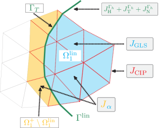
Figure 2. Domain of definition of stabilization terms on the piecewise linear reference geometry ($q=1$). Facets in $\mathcal{F}^{1}$ are indicated by red dashed lines.

Next we introduce stabilization terms on the discrete interface. The first two terms are strong analogs of the classical Nitsche terms commonly found in unfitted methods for interface problems [27, 31]. For $\bar{\mu}=(\mu_{1}+\mu_{2})/2$ we define

$$J_{\mathrm{H}}^{\Gamma_{h}}\left(u_{h},v_{h}\right) :=\frac{\bar{\mu}}{h}\int\limits_{\Gamma_{h}}\llbracket u_{h}\rrbracket_{\Gamma_{h}}\llbracket v_{h}\rrbracket_{\Gamma_{h}}\mathrm{d}S_{\Gamma_{h}},$$

$$J_{\mathrm{N}}^{\Gamma_{h}}\left(u_{h},v_{h}\right) :=h\int\limits_{\Gamma_{h}}\llbracket\mu\nabla u_{h}\rrbracket_{\Gamma_{h}}\cdot n_{\Gamma_{h}}\llbracket\mu\nabla v_{h}\rrbracket_{\Gamma_{h}}\cdot n_{\Gamma_{h}}\;\mathrm{d}S_{\Gamma_{h}}.$$

Additionally, we will stabilize the jump of the tangential gradient

$$J_{\mathrm{T}}^{\Gamma_{h}}\left(u_{h},v_{h}\right):=h\bar{\mu}\int\limits_{\Gamma_{h}}\llbracket\nabla_{\Gamma_{h}}u_{h}\rrbracket_{\Gamma_{h}}\llbracket\nabla_{\Gamma_{h}}v_{h}\rrbracket_{\Gamma_{h}}\mathrm{d}S_{\Gamma_{h}}.$$

The need for this penalty arises due to the nonconformity $V_{h,\Theta}^{\Gamma}\nsubseteq H^{1}(\Omega)$ as we will see later in Lemma 4. We combine the stabilization on the interface into

$$J^{\Gamma_{h}}\left(\cdot,\cdot\right):=\gamma_{\mathrm{IF}}\left(J_{\mathrm{H}}^{\Gamma_{h}}\left(\cdot,\cdot\right)+J_{\mathrm{N}}^{\Gamma_{h}}\left(\cdot,\cdot\right)+J_{\mathrm{T}}^{\Gamma_{h}}\left(\cdot,\cdot\right)\right),$$ (28)

where $\gamma_{\mathrm{IF}}$ is some positive parameter which we will set equal to one for the analysis. Whereas the previous terms would be consistent on the exact geometry for sufficiently smooth solutions of (1)-(3), we now introduce a weakly inconsistent Tikhonov term:

$$J_{\alpha}\left(u_{h},v_{h}\right):=h^{2q}\sum\limits_{i=1,2}\alpha_{1}(u_{h,i},v_{h,i})_{\Omega_{i,h}^{+}}+\alpha_{2}(\nabla u_{h,i},\nabla v_{h,i})_{\Omega_{i,h}^{+}},$$ (29)

for some $\alpha_{i}>0,i=1,2$. A weaker version of this stabilization only involving the $L^{2}$-norm has been utilized previously in the context of unique continuation problems in e.g. [7, 15]. Here we require additionally control over the gradient to compensate for geometric errors introduced by imperfect approximation of the interface, i.e. $\operatorname{dist}(\Gamma,\Gamma_{h})\lesssim\mathcal{O}(h^{q+1})$. We remark that it is possible to localize these geometric errors and consequently the corresponding stabilization to a band of elements around the interface by exploiting the locality of $\Theta_{h}$. As this measure did not lead to a significant improvement of the numerical results, we decided to present the technically simpler global stabilization in this paper.
We combine the introduced terms into the primal stabilization:

$$s_{h}(u_{h},v_{h}) :=\tilde{s}_{h}(u_{h},v_{h})+J_{\mathrm{GLS}}\left(u_{h},v_{h}\right),$$

$$\tilde{s}_{h}(u_{h},v_{h}) :=J_{\mathrm{CIP}}\left(u_{h},v_{h}\right)+J_{\alpha}\left(u_{h},v_{h}\right)+J^{\Gamma_{h}}\left(u_{h},v_{h}\right).$$ (30)

The dual stabilization is simply given by

$$s^{\ast}_{h}(z_{h},w_{h}):=(\mu\nabla z_{h},\nabla w_{h})_{\Omega}.$$ (31)

[Discretization space for dual variable] For the unique continuation problem the dual variable $z_{h}$ simply approximates zero and is therefore taken from the space $V_{h,\Theta}^{0}$ which solely contains functions that are continuous over the interface. However, for control problems as considered in [18] the dual variable approximates the control. Following [25], the control variable of minimal $L^{2}$-norm solves the homogeneous adjoint problem which inherits the discontinuous coefficients of the original problem. Consequently, the latter then has to be discretized using a subspace of $V_{h,\Theta}^{\Gamma}$. We have extended our error analysis to cover this case and arrived at the same final results. Here we present the slightly simpler version using a continuous variable $z_{h}$, yet we point out that the mentioned extension could pave the way to include interfaces in the control problem considered in [18].

3.2.1. Norms

For the error analysis we introduce the norms

$$\left\lVert v_{h}\right\rVert_{s_{h}}:=s_{h}(v_{h},v_{h})^{1/2},\;v_{h}\in V_{h,\Theta}^{\Gamma},\quad\left\lVert w_{h}\right\rVert_{s^{\ast}_{h}}:=s_{h}^{\ast}(w_{h},w_{h})^{1/2},\;w_{h}\in V_{h,\Theta}^{0}.$$ (32)

For $\alpha_{1}>0$ it is clear that $\left\lVert\cdot\right\rVert_{s_{h}}$ is indeed a norm on $V_{h,\Theta}^{\Gamma}$. On the product space $V_{h,\Theta}^{\Gamma}\times V_{h,\Theta}^{0}$ we define the norm

$$|\|(v_{h},w_{h})\||^{2}:=\left\lVert v_{h}\right\rVert_{s_{h}}^{2}+\left\lVert v_{h}\right\rVert_{\omega}^{2}+\left\lVert w_{h}\right\rVert_{s_{h}^{\ast}}^{2}.$$ (33)

Note in passing that combining Friedrich’s inequality with continuity of the data extension yields

$$g(v_{h},w_{h}) \lesssim\left\lVert\delta u_{\omega}\right\rVert_{\omega}\left\lVert v_{h}\right\rVert_{\omega}+\left\lVert\delta f_{h}\right\rVert_{\Omega_{1,h}\cup\Omega_{2,h}}\left\lVert w_{h}\right\rVert_{\Omega}$$

$$+J_{\mathrm{GLS}}\left(\mathcal{L}v_{h},\mathcal{L}v_{h}\right)^{1/2}h\left\lVert\delta f_{h}\right\rVert_{\Omega_{1,h}\cup\Omega_{2,h}}\lesssim\delta|\|(v_{h},w_{h})\||.$$ (34)

Moreover, we will frequently make use of the common notation

$$\left\lVert v_{h}\right\rVert_{\frac{1}{2},h,\Gamma_{h}}^{2}:=h^{-1}\left\lVert v_{h}\right\rVert_{\Gamma_{h}}^{2},\qquad\left\lVert v_{h}\right\rVert_{-\frac{1}{2},h,\Gamma_{h}}^{2}:=h\left\lVert v_{h}\right\rVert_{\Gamma_{h}}^{2}.$$ (35)

For measuring smoothness of the exact solution let us also define

$$\left\lVert u\right\rVert_{q}:=\left\lVert u\right\rVert_{H^{q+1}(\Omega_{1}\cup\Omega_{2})}+\left\lVert u\right\rVert_{W^{3,\infty}(\Omega_{1}\cup\Omega_{2})}.$$ (36)

By Sobolev embedding theorems the second term in (36) involving the infinity norm can be omitted for $q\geqslant 4$ in dimensions $d\leqslant 3$.

3.2.2. Stability, consistency and continuity

We record some elementary properties of the introduced variational forms. [Consistency] Let $u$ be a solution of (1)-(3). Then

$$A(u,v_{h})=\ell(v_{h}),\;\text{ for all }v_{h}\in V_{h,\Phi_{h}}^{0}.$$

Proof.

Follows analogously to [31, Lemma 5.7]. ∎

Further note that

$$B_{h}[(u_{h},z_{h}),(u_{h},-z_{h})]=\left\lVert u_{h}\right\rVert_{s_{h}}^{2}+\left\lVert u_{h}\right\rVert_{\omega}^{2}+\left\lVert z_{h}\right\rVert^{2}_{s_{h}^{\ast}}=|\|(u_{h},z_{h})\|||\|(u_{h},-z_{h})\||.$$

Hence,

$$\sup_{(v_{h},w_{h})\in V_{h,\Theta}^{\Gamma}\times V_{h,\Theta}^{0}}\frac{B_{h}[(u_{h},z_{h}),(v_{h},w_{h})]}{|\|(v_{h},w_{h})\||}\gtrsim|\|(u_{h},z_{h})\||.$$ (37)

The bilinear form $A_{h}$ is also continuous in the defined norms. [Continuity] For $v\in H^{1}(\Omega_{1,h}\cup\Omega_{2,h})+V_{h,\Theta}^{\Gamma}$ and $w_{h}\in V_{h,\Theta}^{0}$ we have

$$A_{h}(v,w_{h})\lesssim\left\lVert w_{h}\right\rVert_{s^{\ast}_{h}}\left(\left\lVert\sqrt{\mu}\nabla v\right\rVert_{\Omega_{1,h}\cup\Omega_{2,h}}+\left\lVert v\right\rVert_{\Omega_{1,h}\cup\Omega_{2,h}}+\left\lVert\llbracket v\rrbracket\right\rVert_{\frac{1}{2},h,\Gamma_{h}}\right).$$

Proof.

Using (19), $w_{h}\in V_{h,\Theta}^{0}$ (in particular it is univalued and smooth inside elements) and finally (18) we obtain

$$\sum\limits_{i=1,2}\sum\limits_{T\in\Gamma_{T}}h\left\lVert\nabla w_{h,i}\right\rVert_{\Theta_{h}(\Gamma_{T})}^{2}\lesssim\sum\limits_{T\in\mathcal{T}_{h}}\left(\left\lVert\nabla w_{h}\right\rVert^{2}_{\Theta_{h}(T)}+h^{2}\left\lVert\nabla w_{h}\right\rVert^{2}_{H^{1}(\Theta_{h}(T))}\right)\lesssim\left\lVert w_{h}\right\rVert_{s^{\ast}_{h}}^{2}.$$

Hence, the claim follows in view of

$$N_{h}^{c}(v,w_{h})\lesssim\left(\sum\limits_{i=1,2}\sum\limits_{T\in\Gamma_{T}}h\left\lVert\nabla w_{h,i}\right\rVert_{\Theta_{h}(\Gamma_{T})}^{2}\right)^{1/2}\left\lVert\llbracket v\rrbracket\right\rVert_{\frac{1}{2},h,\Gamma_{h}}.$$

∎

3.2.3. Geometry errors for bilinear and linear forms

We recall [31, Lemma 5.10] in which the geometric errors for the standard unfitted Nitsche formulation have been analyzed. For $u\in H^{1}(\Omega_{1}\cup\Omega_{2})$ and $w_{h}\in V_{h,\Theta}^{0}$ set $\tilde{u}:=u\circ\Phi_{h}$ and $\tilde{w}_{h}=w_{h}\circ\Phi_{h}^{-1}$.

1. The geometrical consistency error for the bilinear form in the bulk is bounded by

   $$\left\lvert a(u,\tilde{w}_{h})-a_{h}(\tilde{u},w_{h})\right\rvert\lesssim h^{q}\sum\limits_{i=1,2}\left\lVert\tilde{u}_{i}\right\rVert_{H^{1}(\Omega_{i,h})}\left\lVert w_{h}\right\rVert_{H^{1}(\Omega)}\lesssim h^{q}\left\lVert u\right\rVert_{H^{1}(\Omega_{1}\cup\Omega_{2})}\left\lVert w_{h}\right\rVert_{s_{h}^{\ast}}.$$

2. And for the linear form

   $$\left\lvert\ell(\tilde{w}_{h})-\ell_{h}(w_{h})\right\rvert\lesssim h^{q}\left\lVert f\right\rVert_{W^{1,\infty}(\Omega_{1}\cup\Omega_{2})}\left\lVert w_{h}\right\rVert_{\Omega}\lesssim h^{q}\left\lVert u\right\rVert_{W^{3,\infty}(\Omega_{1}\cup\Omega_{2})}\left\lVert w_{h}\right\rVert_{s_{h}^{\ast}},$$

   where the second inequality assumes that $u$ solves (1).

3.3. Unfitted interpolation

To derive error estimates in the next Section 4, we need to be able to compare the exact solution of (1)-(3) with an approximant in our unfitted curved finite element space. Since we are primarily interested in the case of a possibly underresolved geometry, we introduce

Assumption 2.

Let $1\leqslant q\leqslant p$.

Under this assumption it follows thanks to [31, Theorem 3.12] that $\Psi$ induces a family of (curved) finite elements in the sense of Bernardi [2] to which the interpolation theory developed in the latter paper can be applied. We then obtain from [2, Corollary 4.1] the existence of an interpolation operator $I_{h}:H^{\ell}(\Omega)\rightarrow V_{h,\Psi}$ with optimal approximation properties. For $v\in H^{\ell}(\Omega)$ it holds that

$$\left(\sum\limits_{T\in\mathcal{T}_{h}}\left\lvert v-I_{h}v\right\rvert_{H^{m}(\Psi(T))}^{2}\right)^{1/2}\lesssim h^{\ell-m}\left\lVert v\right\rVert_{H^{\ell}(\Omega)}$$ (38)

for $0\leqslant m\leqslant\ell\leqslant q+1$. To define an unfitted interpolation operator, we use standard techniques, see e.g. [27, 37, 31]. We define

$$I_{h}^{\Gamma}:L^{2}(\Omega_{1}\cup\Omega_{2})\rightarrow V_{h,\Psi}^{\Gamma},\quad I_{h}^{\Gamma}u=(R_{1}^{+}I_{h}\mathcal{E}_{1}R_{1}u,R_{2}^{+}I_{h}\mathcal{E}_{2}R_{2}u).$$ (39)

Sometimes we will refer to the components by $(I_{h}^{\Gamma}u)_{i}:=R_{i}^{+}I_{h}\mathcal{E}_{i}R_{i}u$. Since $(I_{h}^{\Gamma}u)_{i}$ will in the following only appear on domains which are part of of the active mesh $\mathcal{T}_{h}^{i}$ on which the restriction $R_{i}^{+}$ amounts to the identity, we will drop $R_{i}^{+}$ from now on to ease notation. We denote by $I_{h}^{0}:H^{1}_{0}(\Omega)\rightarrow V_{h,\Psi}^{0}$ the interpolation operator into the standard (curved) spaces with homogeneous Dirichlet boundary conditions on $\partial\Omega$, see [2, Theorem 5.1]. We then obtain the usual interpolation results. [Unfitted interpolation] Let $u\in H^{\ell}(\Omega_{1}\cup\Omega_{2})$ and $1\leqslant m\leqslant\ell\leqslant q+1$.

1. We have:

   $$\left\lVert(u-I_{h}^{\Gamma}u)\circ\Phi_{h}\right\rVert_{L^{2}(\Omega_{1,h}\cup\Omega_{2,h})}\sim\left\lVert u-I_{h}^{\Gamma}u\right\rVert_{L^{2}(\Omega_{1}\cup\Omega_{2})}\lesssim h^{\ell}\left\lVert u\right\rVert_{H^{\ell}(\Omega_{1}\cup\Omega_{2})}.$$

2. We have:

   $$\left\lVert\nabla(u\circ\Phi_{h}-I_{h}^{\Gamma}u\circ\Phi_{h})\right\rVert_{L^{2}(\Omega_{1,h}\cup\Omega_{2,h})}\sim\left\lVert\nabla(u-I_{h}^{\Gamma}u)\right\rVert_{L^{2}(\Omega_{1}\cup\Omega_{2})}\lesssim h^{\ell-1}\left\lVert u\right\rVert_{H^{\ell}(\Omega_{1}\cup\Omega_{2})}.$$

3. For $i=1,2$ it holds

   $$\left\lVert(\mathcal{E}_{i}R_{i}u-I_{h}\mathcal{E}_{i}R_{i}u)\circ\Phi_{h}\right\rVert_{\frac{1}{2},h,\Gamma_{h}}\lesssim h^{\ell-1}\left\lVert u\right\rVert_{H^{\ell}(\Omega_{i})}.$$

4. For $i=1,2$ and $m\geqslant 2$ it holds

   $$\left\lVert\nabla(\mathcal{E}_{i}R_{i}u-I_{h}\mathcal{E}_{i}R_{i}u)\circ\Phi_{h}\right\rVert_{-\frac{1}{2},h,\Gamma_{h}}\lesssim h^{\ell-1}\left\lVert u\right\rVert_{H^{\ell}(\Omega_{i})}.$$

5. For $i=1,2$ and $m\geqslant 2$ we have

   $$\sum\limits_{T\in\mathcal{T}_{h}^{i}}h^{2}\left\lVert(\mathcal{E}_{i}R_{i}u-I_{h}\mathcal{E}_{i}R_{i}u)\circ\Phi_{h}\right\rVert_{H^{2}(\Theta_{h}(T))}^{2}\lesssim h^{2(\ell-1)}\left\lVert u\right\rVert_{H^{\ell}(\Omega_{i})}^{2}.$$

Proof.

The proofs of statements (a)-(d) are standard, see [27, 37] for the case of a piecewise linear reference geometry and [31, 32] for higher order involving the mapping. We only show statement (e), which follows by applying Lemma 2.5 and the interpolation result (38):

$$\sum\limits_{T\in\mathcal{T}_{h}^{i}}h^{2}\left\lVert(\mathcal{E}_{i}R_{i}u-I_{h}\mathcal{E}_{i}R_{i}u)\circ\Phi_{h}\right\rVert_{H^{2}(\Theta_{h}(T))}^{2}\lesssim\sum\limits_{T\in\mathcal{T}_{h}^{i}}h^{2}\left\lVert\mathcal{E}_{i}R_{i}u-I_{h}\mathcal{E}_{i}R_{i}u\right\rVert_{H^{2}(\Psi_{h}(T))}^{2}$$

$$\lesssim h^{2(\ell-1)}\left\lVert u\right\rVert_{H^{\ell}(\Omega_{i})}^{2}\;\text{ for }2\leqslant m\leqslant\ell\leqslant q+1.$$

∎

As a consequence of the interpolation bounds, the continuity result of Lemma 37, and the geometry error estimate from Lemma 3.2.3 we obtain: Let $u\in H^{q+1}(\Omega_{1}\cup\Omega_{2})$ solve (1)-(3) and $w_{h}\in V_{h,\Theta}^{0}$. Then

$$\left\lvert A(u,w_{h}\circ\Phi_{h}^{-1})-A_{h}(I_{h}^{\Gamma}u\circ\Phi_{h},w_{h})\right\rvert\lesssim h^{q}\left\lVert u\right\rVert_{H^{q+1}(\Omega_{1}\cup\Omega_{2})}\left\lVert w_{h}\right\rVert_{s_{h}^{\ast}}.$$

Proof.

Since $\Phi_{h}(\Omega_{i,h})=\Omega_{i}$ we have $(\mathcal{E}_{i}R_{i}u)\circ\Phi_{h}|_{\Omega_{i,h}}=(R_{i}u)\circ\Phi_{h}|_{\Omega_{i,h}}$ and similarly on $\Gamma_{h}$. Using this along with $N^{c}(u,w_{h}\circ\Phi_{h}^{-1})=N_{h}^{c}(u\circ\Phi_{h},w_{h})=0$ for $u$ solving (2) yields

$$\left\lvert A(u,w_{h}\circ\Phi_{h}^{-1})-A_{h}(I_{h}^{\Gamma}u\circ\Phi_{h},w_{h})\right\rvert$$

$$\leqslant\left\lvert a(u,w_{h}\circ\Phi_{h}^{-1})-a_{h}(u\circ\Phi_{h},w_{h})\right\rvert+\left\lvert A_{h}(\mathcal{E}u\circ\Phi_{h}-I_{h}^{\Gamma}u\circ\Phi_{h},w_{h})\right\rvert$$

$$:=\mathrm{I}_{1}+\mathrm{I}_{2}.$$

By Lemma 3.2.3 we have $\mathrm{I}_{1}\lesssim h^{q}\left\lVert u\right\rVert_{H^{1}(\Omega_{1}\cup\Omega_{2})}\left\lVert w_{h}\right\rVert_{s_{h}^{\ast}}$. To estimate $\mathrm{I}_{2}$ we use continuity of $A_{h}(\cdot,\cdot)$, see Lemma 37, and the interpolation estimates from Lemma 39:

$$\mathrm{I}_{2} \lesssim\left\lVert w_{h}\right\rVert_{s_{h}^{\ast}}\Big{(}\sum\limits_{i=1,2}\left\lVert(\mathcal{E}_{i}R_{i}u-I_{h}\mathcal{E}_{i}R_{i}u)\circ\Phi_{h})\right\rVert_{H^{1}(\Omega_{i,h})}$$

$$+\left\lVert(\mathcal{E}_{i}R_{i}u-I_{h}\mathcal{E}_{i}R_{i}u)\circ\Phi_{h}\right\rVert_{\frac{1}{2},h,\Gamma_{h}}\Big{)}\lesssim h^{q}\left\lVert w_{h}\right\rVert_{s_{h}^{\ast}}\left\lVert u\right\rVert_{H^{q+1}(\Omega_{1}\cup\Omega_{2})}.$$

∎

We now derive several results related to the consistency of the stabilization. By this we mean that if $u$ solves (1)-(3), then inserting the interpolant $I_{h}^{\Gamma}u\circ\Phi_{h}$ into the stabilization terms should at most lead to an error of $\mathcal{O}(h^{q})$. The first lemma deals with the terms on the interface. [Consistency of interface stabilization] Let $u\in H^{q+1}(\Omega_{1}\cup\Omega_{2})$ solve (1)-(3). Then

1. $J_{\mathrm{N}}^{\Gamma_{h}}\left(I_{h}^{\Gamma}u\circ\Phi_{h},I_{h}^{\Gamma}u\circ\Phi_{h}\right)^{1/2}\lesssim h^{q}\left\lVert u\right\rVert_{H^{q+1}(\Omega_{1}\cup\Omega_{2})}.$

2. $J_{\mathrm{T}}^{\Gamma_{h}}\left(I_{h}^{\Gamma}u\circ\Phi_{h},I_{h}^{\Gamma}u\circ\Phi_{h}\right)^{1/2}\lesssim h^{q}\left\lVert u\right\rVert_{H^{q+1}(\Omega_{1}\cup\Omega_{2})}.$

3. $J_{\mathrm{H}}^{\Gamma_{h}}\left(I_{h}^{\Gamma}u\circ\Phi_{h},I_{h}^{\Gamma}u\circ\Phi_{h}\right)^{1/2}\lesssim h^{q}\left\lVert u\right\rVert_{H^{q+1}(\Omega_{1}\cup\Omega_{2})}.$

Proof.

1. From Lemma 2.5 (b) and $\llbracket\mu\nabla u\rrbracket_{\Gamma}\cdot n_{\Gamma}=\llbracket\mu\nabla\mathcal{E}u\rrbracket_{\Gamma}\cdot n_{\Gamma}=0$ we obtain

   $$J_{\mathrm{N}}^{\Gamma_{h}}\left(I_{h}^{\Gamma}u\circ\Phi_{h},I_{h}^{\Gamma}u\circ\Phi_{h}\right)=h\left\lVert\llbracket\mu\nabla I_{h}^{\Gamma}u\circ\Phi_{h}\rrbracket\cdot n_{\Gamma_{h}}\right\rVert_{\Gamma_{h}}^{2}$$

   $$\lesssim h^{2(q+\frac{1}{2})}\sum\limits_{i=1,2}\left\lVert\nabla(I_{h}^{\Gamma}u)_{i}\right\rVert_{\Gamma}^{2}+h\left\lVert\llbracket\mu\nabla(I_{h}^{\Gamma}u-\mathcal{E}u)\rrbracket\cdot n_{\Gamma}\right\rVert_{\Gamma}^{2}$$

   $$\lesssim h^{2(q+\frac{1}{2})}\sum\limits_{i=1,2}\left\lVert\nabla(I_{h}^{\Gamma}u)_{i}\right\rVert_{\Gamma}^{2}+h\sum\limits_{i=1,2}\left\lVert\nabla(I_{h}^{\Gamma}u-\mathcal{E}u)_{i}\right\rVert_{\Gamma}^{2}:=\mathrm{I}_{1}+\mathrm{I}_{2}.$$

   From Lemma 2.5 (a) and Lemma 39 (d) we obtain

   $$\mathrm{I}_{2}\lesssim\sum\limits_{i=1,2}\left\lVert\nabla(\mathcal{E}_{i}R_{i}u-I_{h}\mathcal{E}_{i}R_{i}u)\circ\Phi_{h}\right\rVert_{-\frac{1}{2},h,\Gamma_{h}}^{2}\lesssim h^{2q}\left\lVert u\right\rVert_{H^{q+1}(\Omega_{1}\cup\Omega_{2})}^{2}.$$

   Similarly, $\mathrm{I}_{1}\lesssim h^{2(q+\frac{1}{2})}\left\lVert u\right\rVert_{H^{q+1}(\Omega_{1}\cup\Omega_{2})}^{2}$, which concludes the proof of (a).

2. Since $u\in H^{q+1}(\Omega_{1}\cup\Omega_{2})$ with $q\geqslant 1$ we are allowed to take the tangential derivative of equation (2) to obtain $\llbracket\nabla_{\Gamma}u\rrbracket_{\Gamma}=0$. Then using Lemma 2.5 (c) yields

   $$J_{\mathrm{T}}^{\Gamma_{h}}\left(I_{h}^{\Gamma}u\circ\Phi_{h},I_{h}^{\Gamma}u\circ\Phi_{h}\right)=h\bar{\mu}\left\lVert\llbracket\nabla_{\Gamma_{h}}I_{h}^{\Gamma}u\circ\Phi_{h}\rrbracket\right\rVert_{\Gamma_{h}}^{2}$$

   $$\lesssim h^{2(q+\frac{1}{2})}\sum\limits_{i=1,2}\left\lVert\nabla(I_{h}^{\Gamma}u)_{i}\right\rVert_{\Gamma}^{2}+h\left\lVert\llbracket\nabla_{\Gamma}I_{h}^{\Gamma}u\rrbracket\right\rVert_{\Gamma}^{2}$$

   $$\sim h^{2(q+\frac{1}{2})}\sum\limits_{i=1,2}\left\lVert\nabla(I_{h}^{\Gamma}u)_{i}\right\rVert_{\Gamma}^{2}+h\left\lVert\llbracket\nabla_{\Gamma}(I_{h}^{\Gamma}u-\mathcal{E}u)\rrbracket\right\rVert_{\Gamma}^{2}\lesssim\mathrm{I}_{1}+\mathrm{I}_{2}.$$

   The terms $\mathrm{I}_{1}$ and $\mathrm{I}_{2}$ are the same as the ones already estimated in (a).

3. As $\Phi_{h}(\Gamma_{h})=\Gamma$ we have $0=\llbracket u\rrbracket_{\Gamma}=\llbracket\mathcal{E}u\rrbracket_{\Gamma}=\llbracket\mathcal{E}u\circ\Phi_{h}\rrbracket_{\Gamma_{h}}$. This allows to skip the transformation step to the exact interface that was necessary in part (a)-(b). Hence, by applying Lemma 39 (c):

   $$J_{\mathrm{H}}^{\Gamma_{h}}\left(I_{h}^{\Gamma}u\circ\Phi_{h},I_{h}^{\Gamma}u\circ\Phi_{h}\right)=\frac{\bar{\mu}}{h}\left\lVert\llbracket I_{h}^{\Gamma}u\circ\Phi_{h}\rrbracket_{\Gamma_{h}}\right\rVert_{\Gamma_{h}}^{2}=\frac{\bar{\mu}}{h}\left\lVert\llbracket I_{h}^{\Gamma}u\circ\Phi_{h}-\mathcal{E}u\circ\Phi_{h}\rrbracket_{\Gamma_{h}}\right\rVert_{\Gamma_{h}}^{2}$$

   $$\lesssim\sum\limits_{i=1,2}\left\lVert(\mathcal{E}_{i}R_{i}u-I_{h}\mathcal{E}_{i}R_{i}u)\circ\Phi_{h}\right\rVert_{\frac{1}{2},h,\Gamma_{h}}^{2}\lesssim h^{2q}\left\lVert u\right\rVert_{H^{q+1}(\Omega_{1}\cup\Omega_{2})}^{2}.$$

∎

Next we consider the least squares term. [Least-squares term] Let $u\in H^{q+1}(\Omega_{1}\cup\Omega_{2})\cap W^{3,\infty}(\Omega_{1}\cup\Omega_{2})$ solve (1)-(3). Then it holds that

$$\sum\limits_{i=1,2}\sum\limits_{T\in\mathcal{T}_{h}^{i}}h^{2}\left\lVert f_{i,h}-\mathcal{L}(I_{h}^{\Gamma}u\circ\Phi_{h})\right\rVert^{2}_{\Theta_{h}(T_{i})}\lesssim h^{2q}\left\lVert u\right\rVert_{q}^{2}.$$

Proof.

We have

$$\sum\limits_{i=1,2}\sum\limits_{T\in\mathcal{T}_{h}^{i}}h^{2}\left\lVert f_{i,h}-\mathcal{L}(I_{h}^{\Gamma}u\circ\Phi_{h})\right\rVert^{2}_{\Theta_{h}(T_{i})}\lesssim\sum\limits_{i=1,2}\sum\limits_{T\in\mathcal{T}_{h}^{i}}h^{2}\left\lVert f_{i,h}-\mathcal{L}(\mathcal{E}_{i}u_{i}\circ\Phi_{h})\right\rVert^{2}_{\Theta_{h}(T_{i})}$$

$$+\sum\limits_{i=1,2}\sum\limits_{T\in\mathcal{T}_{h}^{i}}h^{2}\left\lVert\mathcal{L}((\mathcal{E}_{i}R_{i}u-I_{h}\mathcal{E}_{i}R_{i}u)\circ\Phi_{h})\right\rVert^{2}_{\Theta_{h}(T)}$$

$$\lesssim\sum\limits_{i=1,2}\sum\limits_{T\in\mathcal{T}_{h}^{i}}h^{2}\left\lVert f_{i,h}-\mathcal{L}(\mathcal{E}_{i}u_{i}\circ\Phi_{h})\right\rVert^{2}_{\Theta_{h}(T_{i})}+h^{2q}\left\lVert u\right\rVert_{H^{q+1}(\Omega_{1}\cup\Omega_{2})}^{2},$$

where Lemma 39 (e) has been applied. To treat the remaining term further, we employ Lemma 2.5 (a) and the triangle inequality to split

$$\sum\limits_{i=1,2}\sum\limits_{T\in\mathcal{T}_{h}^{i}}h^{2}\left\lVert f_{i,h}-\mathcal{L}(\mathcal{E}_{i}u_{i}\circ\Phi_{h})\right\rVert^{2}_{\Theta_{h}(T_{i})}$$

$$\lesssim\sum\limits_{i=1,2}\sum\limits_{T\in\mathcal{T}_{h}^{i}}h^{2}\left\lVert f_{i,h}\circ\Phi_{h}^{-1}-\mathcal{L}(\mathcal{E}_{i}u_{i}\circ\Phi_{h})\circ\Phi_{h}^{-1}\right\rVert^{2}_{\Psi_{h}(T_{i})}$$

$$\lesssim\sum\limits_{i=1,2}\sum\limits_{T\in\mathcal{T}_{h}^{i}}h^{2}\left\lVert f_{i,h}\circ\Phi_{h}^{-1}-f_{i,h}\right\rVert^{2}_{\Psi_{h}(T_{i})}+\sum\limits_{i=1,2}\sum\limits_{T\in\mathcal{T}_{h}^{i}}h^{2}\left\lVert f_{i,h}-\mathcal{L}(\mathcal{E}_{i}u_{i}\circ\Phi_{h})\circ\Phi_{h}^{-1}\right\rVert^{2}_{\Psi_{h}(T_{i})}$$

$$:=\mathrm{J}_{1}+\mathrm{J}_{2}.$$

From Lemma 2.5 (a) we obtain

$$\mathrm{J}_{1}\lesssim h^{2(q+2)}\sum\limits_{i=1,2}\left\lVert\nabla f_{i,h}\right\rVert_{\infty,\Omega}^{2}\lesssim h^{2(q+2)}\left\lVert f\right\rVert_{W^{1,\infty}(\Omega_{1}\cup\Omega_{2})}^{2}\lesssim h^{2(q+2)}\left\lVert u\right\rVert_{W^{3,\infty}(\Omega_{1}\cup\Omega_{2})}^{2}$$

by our smoothness assumption on the data extension. To treat $\mathrm{J}_{2}$ we note that as $\Psi(T_{i})\subset\Omega_{i}$ by construction it holds

$$f_{i,h}|_{\Psi(T_{i})}=f_{i}=\mathcal{L}R_{i}u=(\mathcal{L}\mathcal{E}_{i}R_{i}u)|_{\Psi(T_{i})}.$$

Hence, we obtain from Lemma 2.5 (d)

$$\mathrm{J}_{2} =\sum\limits_{i=1,2}\sum\limits_{T\in\mathcal{T}_{h}^{i}}h^{2}\left\lVert\mathcal{L}(\mathcal{E}_{i}R_{i}u)-\mathcal{L}(\mathcal{E}_{i}u_{i}\circ\Phi_{h})\circ\Phi_{h}^{-1}\right\rVert^{2}_{\Psi_{h}(T_{i})}\lesssim h^{2q}\left\lVert u\right\rVert_{H^{2}(\Omega_{1}\cup\Omega_{2})}^{2},$$

which concludes the argument. ∎

We also have to estimate the continuous interior penalty term. The proof is similar to [29, Lemma 13] where a related estimate for a facet-based ghost penalty stabilization, which is a localized form of continuous interior penalty (possibly including higher order jumps), has been established. To this end, an interpolation operator which maps directly into $V_{h,\Theta}^{\Gamma}$ was constructed. Note that our interpolator $I_{h}^{\Gamma}$ maps to $V_{h,\Psi}^{\Gamma}$ instead so that we first compose with $\Phi_{h}$ to obtain $I_{h}^{\Gamma}u\circ\Phi_{h}\in V_{h,\Theta}^{\Gamma}$. [Continuous interior penalty] Let $u\in H^{q+1}(\Omega_{1}\cup\Omega_{2})\cap W^{3,\infty}(\Omega_{1}\cup\Omega_{2})$ solve (1)-(3). Then it holds that

$$J_{\mathrm{CIP}}\left(I_{h}^{\Gamma}u\circ\Phi_{h},I_{h}^{\Gamma}u\circ\Phi_{h}\right)^{1/2}\lesssim h^{q}\left\lVert u\right\rVert_{q}.$$

Proof.

Since $\mathcal{E}_{i}R_{i}u\in H^{2}(\Omega)$ we have

$$J_{\mathrm{CIP}}\left(I_{h}^{\Gamma}u\circ\Phi_{h},I_{h}^{\Gamma}u\circ\Phi_{h}\right)=\sum\limits_{i=1,2}\sum\limits_{F\in\mathcal{F}^{i}}h\!\!\!\!\int\limits_{\Theta_{h}(F)}\!\!\!\!\mu_{i}\left\lVert\llbracket\nabla(\mathcal{E}_{i}R_{i}u-(I_{h}\mathcal{E}_{i}R_{i}u)\circ\Phi_{h})\rrbracket_{\Theta_{h}(F)}\cdot n\right\rVert^{2}\!\!\mathrm{d}S$$

$$\lesssim\sum\limits_{i=1,2}\sum\limits_{T\in\mathcal{T}_{h}^{i}}h\left\lVert\nabla(\mathcal{E}_{i}R_{i}u-(I_{h}\mathcal{E}_{i}R_{i}u)\circ\Phi_{h})\right\rVert_{\partial\Theta_{h}(T)}^{2}$$

$$\lesssim\sum\limits_{i=1,2}\sum\limits_{T\in\mathcal{T}_{h}^{i}}\left\lVert\mathcal{E}_{i}R_{i}u-(I_{h}\mathcal{E}_{i}R_{i}u)\circ\Phi_{h}\right\rVert_{H^{1}(\Theta_{h}(T))}^{2}+h^{2}\left\lVert\mathcal{E}_{i}R_{i}u-(I_{h}\mathcal{E}_{i}R_{i}u)\circ\Phi_{h}\right\rVert_{H^{2}(\Theta_{h}(T))}^{2}$$

$$:=\mathrm{I}_{1}+\mathrm{I}_{2}.$$

From Lemma 2.5 (c) and Lemma 39 (e) we obtain

$$\mathrm{I}_{2} \lesssim\sum\limits_{i=1,2}\sum\limits_{T\in\mathcal{T}_{h}^{i}}h^{2}\left\lVert\mathcal{E}_{i}R_{i}u-(\mathcal{E}_{i}R_{i}u)\circ\Phi_{h}\right\rVert_{H^{2}(\Theta_{h}(T))}^{2}+h^{2}\left\lVert(\mathcal{E}_{i}R_{i}u-I_{h}\mathcal{E}_{i}R_{i}u)\circ\Phi_{h}\right\rVert_{H^{2}(\Theta_{h}(T))}^{2}$$

$$\lesssim h^{2q}\left\lVert u\right\rVert_{W^{3,\infty}(\Omega_{1}\cup\Omega_{2})}^{2}+h^{2q}\left\lVert u\right\rVert_{H^{q+1}(\Omega_{1}\cup\Omega_{2})}^{2}.$$

The term $\mathrm{I}_{1}$ is estimated similarly by appealing to Lemma 2.5 (b) and Lemma 39 (a)-(b). ∎

Let us define

$$S_{h}(I_{h}^{\Gamma}u\circ\Phi_{h}):=\sum\limits_{i=1,2}\sum\limits_{T\in\mathcal{T}_{h}^{i}}h^{2}\left\lVert f_{i,h}-\mathcal{L}(I_{h}^{\Gamma}u\circ\Phi_{h})\right\rVert^{2}_{\Theta_{h}(T_{i})}+J_{\alpha}\left(I_{h}^{\Gamma}u\circ\Phi_{h},I_{h}^{\Gamma}u\circ\Phi_{h}\right)$$

$$+J_{\mathrm{CIP}}\left(I_{h}^{\Gamma}u\circ\Phi_{h},I_{h}^{\Gamma}u\circ\Phi_{h}\right)+J^{\Gamma_{h}}\left(I_{h}^{\Gamma}u\circ\Phi_{h},I_{h}^{\Gamma}u\circ\Phi_{h}\right)$$

Then by combining the previous results we obtain: Let $u\in H^{q+1}(\Omega_{1}\cup\Omega_{2})\cap W^{3,\infty}(\Omega_{1}\cup\Omega_{2})$ solve (1)-(3). Then

$$S_{h}(I_{h}^{\Gamma}u\circ\Phi_{h})\lesssim h^{2q}\left\lVert u\right\rVert_{q}^{2}.$$

Proof.

This follows from Lemma 2, Lemma 2, Lemma 2 and

$$J_{\alpha}\left(I_{h}^{\Gamma}u\circ\Phi_{h},I_{h}^{\Gamma}u\circ\Phi_{h}\right)\lesssim h^{2q}\left\lVert u\right\rVert_{H^{1}(\Omega_{1}\cup\Omega_{2})}^{2}.$$

∎

4. Error analysis

Thanks to the results established in the previous two sections, the usual error analysis for methods based on the framework in [5] can be applied. First we establish convergence of the error in the stabilization norm $|\|\cdot\||$, see Corollary 4, then we utilize the conditional stability estimate to deduce convergence in the target domain, see Theorem 4.5. We start by analyzing the discretization error.

Proposition 1.

Let $u\in H^{q+1}(\Omega_{1}\cup\Omega_{2})\cap W^{3,\infty}(\Omega_{1}\cup\Omega_{2})$ be the exact solution of (1)-(4). Let $(u_{h},z_{h})\in V_{h,\Theta}^{\Gamma}\times V_{h,\Theta}^{0}$ be the solution of (25). Then

$$|\|(u_{h}-I_{h}^{\Gamma}u\circ\Phi_{h},z_{h})\||\lesssim h^{q}\left\lVert u\right\rVert_{q}+\delta.$$

Proof 4.1.

In view of the inf-sup condition (37), it suffices to show that

$$B_{h}[(u_{h}-I_{h}^{\Gamma}u\circ\Phi_{h},z_{h}),(v_{h},w_{h})]\lesssim|\|(v_{h},w_{h})\||(h^{q}\left\lVert u\right\rVert_{q}+\delta)$$

for all $(v_{h},w_{h})\in V_{h,\Theta}^{\Gamma}\times V_{h,\Theta}^{0}$. Using first order optimality (25) and consistency (Lemma 3.2.2) yields

$$B_{h}[(u_{h}-I_{h}^{\Gamma}u\circ\Phi_{h},z_{h}),(v_{h},w_{h})]=(u-I_{h}^{\Gamma}u\circ\Phi_{h},v_{h})_{\omega}+\ell_{h}(w_{h})+g(v_{h},w_{h})$$

$$+\sum\limits_{i=1,2}\sum\limits_{T\in\mathcal{T}_{h}^{i}}h^{2}(f_{i,h},\mathcal{L}v_{h,i})_{\Theta_{h}(T_{i})}-s_{h}(I_{h}^{\Gamma}u\circ\Phi_{h},v_{h})-A_{h}(I_{h}^{\Gamma}u\circ\Phi_{h},w_{h})$$

$$=\underbrace{(u-I_{h}^{\Gamma}u\circ\Phi_{h},v_{h})_{\omega}}_{I_{1}}+\underbrace{[\ell_{h}(w_{h})-\ell(w_{h}\circ\Phi_{h}^{-1})]}_{I_{2}}+\underbrace{[A(u,w_{h}\circ\Phi_{h}^{-1})-A_{h}(I_{h}^{\Gamma}u\circ\Phi_{h},w_{h})]}_{I_{3}}$$

$$+\underbrace{\left[\sum\limits_{i=1,2}\sum\limits_{T\in\mathcal{T}_{h}^{i}}h^{2}(f_{i,h}-\mathcal{L}I_{h}^{\Gamma}u\circ\Phi_{h},\mathcal{L}v_{h,i})_{\Theta_{h}(T_{i})}-\tilde{s}_{h}(I_{h}^{\Gamma}u\circ\Phi_{h},v_{h})\right]}_{I_{4}}+\underbrace{g(v_{h},w_{h})}_{I_{5}}.$$

We consider the terms $\mathrm{I}_{j}$ separately.

• Recall that we assume $\Phi_{h}|_{\omega}=\mathrm{id}$ and $\omega\subset\Omega_{i}$ for exactly one $i\in\{1,2\}$ so that from the interpolation estimates in Lemma 39 we obtain

  $$\mathrm{I}_{1}\lesssim\left\lVert v_{h}\right\rVert_{\omega}\left\lVert u-I_{h}^{\Gamma}u\right\rVert_{\omega}\lesssim h^{q+1}\left\lVert v_{h}\right\rVert_{\omega}\left\lVert u\right\rVert_{H^{q+1}(\Omega_{1}\cup\Omega_{2})}.$$

• From Lemma 3.2.3 and Lemma 3.3 we have

  $$\mathrm{I}_{2}+\mathrm{I}_{3}\lesssim h^{q}\left\lVert u\right\rVert_{q}\left\lVert w_{h}\right\rVert_{s_{h}^{\ast}}.$$

• For the second to last term we apply Corollary 3.3 to obtain

  $$\mathrm{I}_{4}\lesssim S_{h}(I_{h}^{\Gamma}u\circ\Phi_{h})^{1/2}\left\lVert v_{h}\right\rVert_{s_{h}}\lesssim h^{q}\left\lVert u\right\rVert_{q}\left\lVert v_{h}\right\rVert_{s_{h}}.$$

• Now only the perturbation remains which has already been estimated in (34).

Combining these estimates yields the claim.

Let $u\in H^{q+1}(\Omega_{1}\cup\Omega_{2})\cap W^{3,\infty}(\Omega_{1}\cup\Omega_{2})$ be the exact solution of (1)-(4). Let $(u_{h},z_{h})\in V_{h,\Theta}^{\Gamma}\times V_{h,\Theta}^{0}$ be the solution of (25). Then

$$|\|(u_{h}-\mathcal{E}u\circ\Phi_{h},z_{h})\||\lesssim h^{q}\left\lVert u\right\rVert_{q}+\delta.$$

Proof 4.2.

By the triangle inequality

$$|\|(u_{h}-\mathcal{E}u\circ\Phi_{h},z_{h})\||\lesssim|\|(u_{h}-I_{h}^{\Gamma}u\circ\Phi_{h},z_{h})\||+|\|((I_{h}^{\Gamma}u-\mathcal{E}u)\circ\Phi_{h},0)\||.$$

The first term has been estimated in Proposition 1 while the approximation error is easily treated by appealing to the interpolation results given in Lemma 39.

Corollary 4 has to be combined with the conditional stability estimate from Corollary 1.2 to deduce convergence rates in the target domain. To this end, we would like to apply the latter to $u-u_{h}\circ\Phi_{h}^{-1}$. Unfortunately, this is not immediately possible as $u_{h}\circ\Phi_{h}^{-1}\notin H^{1}(\Omega)$ due to the use of an unfitted discretization. This can be fixed by adding a corrector function which removes possible jumps across the interface. The next lemma shows that the norm of this correction can be controlled by the stabilization. Let $u\in H^{q+1}(\Omega_{1}\cup\Omega_{2})\cap W^{3,\infty}(\Omega_{1}\cup\Omega_{2})$ be the exact solution of (1)-(4). Let $(u_{h},z_{h})\in V_{h,\Theta}^{\Gamma}\times V_{h,\Theta}^{0}$ be the solution of (25). Let $\varphi\in H^{1}(\Omega_{1})$ be the solution of

$$\left\{\begin{array}[]{rcll}&-\Delta\varphi=0,&\text{ in }\Omega_{1},\\ &\varphi=-\llbracket u_{h}\circ\Phi_{h}^{-1}\rrbracket&\text{ on }\Gamma.\end{array}\right.$$ (40)

Then

$$\left\lVert\varphi\right\rVert_{H^{1}(\Omega_{1})}\lesssim h^{q}\left\lVert u\right\rVert_{q}+\delta.$$

Proof 4.3.

It follows from the Lax-Milgram lemma that

$$\left\lVert\varphi\right\rVert_{H^{1}(\Omega_{1})}\lesssim\left\lVert\llbracket u_{h}\circ\Phi_{h}^{-1}\rrbracket\right\rVert_{H^{1/2}(\Gamma)}.$$

We have to estimate the jump term on the right hand side using convergence of $u_{h}-\mathcal{E}u\circ\Phi_{h}$ in the $|\|\cdot\||$-norm, see Corollary 4. To achieve this, there are two main obstacles to overcome. Firstly, we have to eliminate the $H^{1/2}$-norm. To this end, we apply a Gagliardo-Nirenberg inequality on $\Gamma$ and use $\llbracket u\rrbracket_{\Gamma}=\llbracket\mathcal{E}u\rrbracket_{\Gamma}=0$ and $\llbracket\nabla_{\Gamma}u\rrbracket_{\Gamma}=\llbracket\nabla_{\Gamma}\mathcal{E}u\rrbracket_{\Gamma}=0$ to obtain

$$\left\lVert\llbracket u_{h}\circ\Phi_{h}^{-1}\rrbracket\right\rVert_{H^{1/2}(\Gamma)}^{2} \lesssim\left\lVert\llbracket u_{h}\circ\Phi_{h}^{-1}\rrbracket\right\rVert_{L^{2}(\Gamma)}\left\lVert\llbracket u_{h}\circ\Phi_{h}^{-1}\rrbracket\right\rVert_{H^{1}(\Gamma)}$$

$$\lesssim h^{-1}\left\lVert\llbracket u_{h}\circ\Phi_{h}^{-1}-\mathcal{E}u\rrbracket\right\rVert_{\Gamma}^{2}+h\left\lVert\llbracket\nabla_{\Gamma}(u_{h}\circ\Phi_{h}^{-1}-\mathcal{E}u)\rrbracket\right\rVert_{\Gamma}^{2}.$$

Secondly, we have to transform from the exact interface to its approximation $\Gamma_{h}$ on which the discretization is defined. According to Lemma 2.5 (c), this will lead to an additional geometrical error on the discrete interfaces involving the full gradient, that is

$$\left\lVert\llbracket u_{h}\circ\Phi_{h}^{-1}\rrbracket\right\rVert_{H^{1/2}(\Gamma)}^{2} \lesssim h^{-1}\left\lVert\llbracket u_{h}-\mathcal{E}u\circ\Phi_{h}\rrbracket\right\rVert_{\Gamma_{h}}^{2}+h\left\lVert\llbracket\nabla_{\Gamma_{h}}(u_{h}-\mathcal{E}u\circ\Phi_{h})\rrbracket\right\rVert_{\Gamma_{h}}^{2}$$

$$+h^{2(q+\frac{1}{2})}\sum\limits_{i=1,2}\left\lVert\nabla(u_{h,i}-\mathcal{E}_{i}u_{i}\circ\Phi_{h})\right\rVert_{\Gamma_{h}}^{2}$$

$$\lesssim|\|(u_{h}-\mathcal{E}u\circ\Phi_{h},z_{h})\||^{2}+h^{2(q+\frac{1}{2})}\sum\limits_{i=1,2}(\left\lVert\nabla u_{h,i}\right\rVert_{\Gamma_{h}}^{2}+\left\lVert\nabla\mathcal{E}_{i}u_{i}\right\rVert_{\Gamma}^{2})$$

$$\lesssim(h^{q}\left\lVert u\right\rVert_{q}+\delta)^{2}+h^{2(q+\frac{1}{2})}\sum\limits_{i=1,2}\left\lVert\nabla u_{h,i}\right\rVert_{\Gamma_{h}}^{2}.$$

Here we used that the jumps on the interface are controlled by the stabilization and Corollary 4. We will bound the remaining term in terms of the weak $H^{1}$-penalty using the trace (19) and inverse inequalitites (18):

$$h\left\lVert\nabla u_{h,i}\right\rVert_{\Gamma_{h}}^{2} \lesssim\sum\limits_{T\in\mathcal{T}^{\Gamma}}\left\lVert u_{h,i}\right\rVert_{H^{1}(\Theta_{h}(T))}^{2}+h^{2}\left\lVert u_{h,i}\right\rVert_{H^{2}(\Theta_{h}(T))}^{2}\lesssim\sum\limits_{T\in\mathcal{T}^{\Gamma}}\left\lVert u_{h,i}\right\rVert_{H^{1}(\Theta_{h}(T))}^{2}.$$

Hence,

$$h^{2(q+\frac{1}{2})}\sum\limits_{i=1,2}\left\lVert\nabla u_{h,i}\right\rVert_{\Gamma_{h}}^{2}\lesssim J_{\alpha}\left(u_{h},u_{h}\right)$$

$$\lesssim J_{\alpha}\left(u_{h}-\mathcal{E}u\circ\Phi_{h},u_{h}-\mathcal{E}u\circ\Phi_{h}\right)+h^{2q}\sum\limits_{i=1,2}\left\lVert\mathcal{E}_{i}u_{i}\circ\Phi_{h}\right\rVert_{H^{1}(\Omega)}^{2}\lesssim(h^{q}\left\lVert u\right\rVert_{q}+\delta)^{2}$$

by Corollary 4.

To benefit from the application of the conditional stability estimate, we have to control the terms on the right hand side of (5). In particular, we have to control the residual in the $H^{-1}$-norm, which is ensured by the following lemma. Let $u\in H^{q+1}(\Omega_{1}\cup\Omega_{2})\cap W^{3,\infty}(\Omega_{1}\cup\Omega_{2})$ be the exact solution of (1)-(4). Let $(u_{h},z_{h})\in V_{h,\Theta}^{\Gamma}\times V_{h,\Theta}^{0}$ be the solution of (25). Then for any $w\in H^{1}_{0}(\Omega)$ it holds that

$$a(u-u_{h}\circ\Phi_{h}^{-1},w)\lesssim(h^{q}\left\lVert u\right\rVert_{q}+\delta)\left\lVert w\right\rVert_{H^{1}(\Omega)}.$$

Proof 4.4.

Let us define the shorthand $w_{h}:=w\circ\Phi_{h},\tilde{w}_{h}:=w_{h}\circ\Phi_{h}^{-1}$ and $\tilde{u}=u\circ\Phi_{h}$. Clearly, we have to deduce the claim eventually from Corollary 4 for which we have to transform to the approximate geometry. Thus, the first step in this proof is to show that:

$$a(u-u_{h}\circ\Phi_{h}^{-1},w)\lesssim a_{h}(\tilde{u}-u_{h},w_{h})+(h^{q}\left\lVert u\right\rVert_{q}+\delta)\left\lVert w\right\rVert_{H^{1}(\Omega)}$$ (41)

holds true. To this end, note that $w=\tilde{w}_{h}$, so we have

$$a(u-u_{h}\circ\Phi_{h}^{-1},w)=[a(u,\tilde{w}_{h})-a_{h}(\tilde{u},w_{h})]+[a_{h}(u_{h},w_{h})-a(u_{h}\circ\Phi_{h}^{-1},\tilde{w}_{h})]+a_{h}(\tilde{u}-u_{h},w_{h}).$$

To estimate the first bracket we simply appeal to Lemma 3.2.3 (a). To control the second bracket, the term $J_{\alpha}\left(\cdot,\cdot\right)$ is essential. By definition (29) of this term, Lemma 3.2.3 (a) and Proposition 1 we deduce

$$\left\lvert a_{h}(u_{h},w_{h})-a(u_{h}\circ\Phi_{h}^{-1},\tilde{w}_{h})\right\rvert\lesssim h^{q}\left\lVert w\right\rVert_{H^{1}(\Omega)}\sum\limits_{i=1,2}\left\lVert u_{h,i}\right\rVert_{H^{1}(\Omega_{i,h})}$$

$$\lesssim h^{q}\left\lVert w\right\rVert_{H^{1}(\Omega)}\left(h^{-q}J_{\alpha}\left(u_{h}-I_{h}^{\Gamma}u\circ\Phi_{h},u_{h}-I_{h}^{\Gamma}u\circ\Phi_{h}\right)^{1/2}+\left\lVert I_{h}^{\Gamma}u\circ\Phi_{h}\right\rVert_{H^{1}(\Omega_{1,h}\cup\Omega_{2,h})}\right)$$

$$\lesssim\left\lVert w\right\rVert_{H^{1}(\Omega)}(h^{q}\left\lVert u\right\rVert_{q}+\delta),$$

which shows (41). The next step is to bound $a_{h}(\tilde{u}-u_{h},w_{h})$ by terms which can be controlled by the stabilization. We claim that

$$a_{h}(\tilde{u}-u_{h},w_{h})\lesssim h^{q}\left\lVert w\right\rVert_{H^{1}(\Omega)}\left\lVert u\right\rVert_{q}+\sum\limits_{j=1}^{6}\mathrm{I}_{j},$$ (42)

where

$$\mathrm{I}_{1}:=\sum\limits_{i=1,2}\sum\limits_{T\in\mathcal{T}_{h}^{i}}(\mathcal{L}(\mathcal{E}_{i}R_{i}u\circ\Phi_{h}-u_{h,i}),w\circ\Phi_{h}-(I_{h}^{0}w)\circ\Phi_{h})_{\Theta_{h}(T_{i})}$$

$$\mathrm{I}_{2}:=\sum\limits_{i=1,2}\sum\limits_{F\in\mathcal{F}^{i}}h\int\limits_{\Theta_{h}(F\cap T_{i})}\!\!\!\!\!\mu_{i}\llbracket\nabla(\mathcal{E}_{i}R_{i}u\circ\Phi_{h}-u_{h,i})\rrbracket_{\Theta_{h}(F)}\cdot n\;(w\circ\Phi_{h}-(I_{h}^{0}w)\circ\Phi_{h})\;\mathrm{d}S_{\Theta_{h}(F)}$$

$$\mathrm{I}_{3}:=N^{c}_{h}(u_{h},I_{h}^{0}w\circ\Phi_{h}),\quad\mathrm{I}_{4}:=-s_{h}^{\ast}(z_{h},I_{h}^{0}w\circ\Phi_{h}),\quad\mathrm{I}_{5}:=-(\delta f_{h},I_{h}^{0}w\circ\Phi_{h})_{\Omega_{1,h}\cup\Omega_{2,h}}$$

$$\mathrm{I}_{6}:=\left(\llbracket\mu\nabla(\mathcal{E}u\circ\Phi_{h}-u_{h})\rrbracket\cdot n_{\Gamma_{h}},w\circ\Phi_{h}-I_{h}^{0}w\circ\Phi_{h}\right)_{\Gamma_{h}}.\;$$

To establish (42), we first use consistency

$$\ell(I_{h}^{0}w)=a(u,I_{h}^{0}w),$$

which follows from Lemma 3.2.2. Hence,

$$a_{h}(\tilde{u}-u_{h},w_{h}) =a_{h}(\tilde{u}-u_{h},w\circ\Phi_{h}-I_{h}^{0}w\circ\Phi_{h})-a_{h}(u_{h},I_{h}^{0}w\circ\Phi_{h})$$

$$+[a_{h}(\tilde{u},I_{h}^{0}w\circ\Phi_{h})-a(u,I_{h}^{0}w)]+\ell(I_{h}^{0}w).$$ (43)

By appealing to Lemma 3.2.3 (a) we obtain

$$\left\lvert a_{h}(\tilde{u},I_{h}^{0}w\circ\Phi_{h})-a(u,I_{h}^{0}w)\right\rvert =\left\lvert a(u,(I_{h}^{0}w\circ\Phi_{h})\circ\Phi_{h}^{-1})-a_{h}(\tilde{u},I_{h}^{0}w\circ\Phi_{h})\right\rvert$$

$$\lesssim h^{q}\left\lVert u\right\rVert_{H^{1}(\Omega_{1}\cup\Omega_{2})}\left\lVert w\right\rVert_{H^{1}(\Omega)}.$$

Next we add the first order optimality condition

$$A_{h}(u_{h},I_{h}^{0}w\circ\Phi_{h})+\mathrm{I}_{4}-\ell_{h}(I_{h}^{0}w\circ\Phi_{h})+\mathrm{I}_{5}=0,$$

which follows from (25), to the right hand side of (43). Using that

$$\left\lvert\ell(I_{h}^{0}w)-\ell_{h}(I_{h}^{0}w\circ\Phi_{h})\right\rvert\lesssim h^{q}\left\lVert u\right\rVert_{q}\left\lVert I_{h}^{0}w\circ\Phi_{h}\right\rVert_{\Omega_{1,h}\cup\Omega_{2,h}}\lesssim h^{q}\left\lVert u\right\rVert_{q}\left\lVert w\right\rVert_{H^{1}(\Omega)},$$

as ensured by Lemma 3.2.3 (b) and

$$-a_{h}(u_{h},I_{h}^{0}w\circ\Phi_{h})+A_{h}(u_{h},I_{h}^{0}w\circ\Phi_{h})=\mathrm{I}_{3}$$

yields

$$a_{h}(\tilde{u}-u_{h},w_{h})\lesssim h^{q}\left\lVert u\right\rVert_{q}\left\lVert w\right\rVert_{H^{1}(\Omega)}+a_{h}(\tilde{u}-u_{h},w\circ\Phi_{h}-I_{h}^{0}w\circ\Phi_{h})+\mathrm{I}_{3}+\mathrm{I}_{4}+\mathrm{I}_{5}.$$ (44)

We recognize that the claimed inequality (42) slowly begins to appear. The final step is an element-wise integration by parts of $a_{h}(\tilde{u}-u_{h},w\circ\Phi_{h}-I_{h}^{0}w\circ\Phi_{h})$, which will in particular lead to a boundary term on $\partial\Omega_{i,h}\setminus\partial\Omega$ that can be written as $\mathrm{I}_{6}$. Hence, integration by parts yields

$$a_{h}(\tilde{u}-u_{h},w\circ\Phi_{h}-I_{h}^{0}w\circ\Phi_{h})=\mathrm{I}_{1}+\mathrm{I}_{2}+\mathrm{I}_{6}.$$

Inserting this identity into (44) establishes (42).

In view of (41) and (42) it now remains to show that

$$\sum\limits_{j=1}^{6}\mathrm{I}_{j}\lesssim\left\lVert w\right\rVert_{H^{1}(\Omega)}(h^{q}\left\lVert u\right\rVert_{q}+\delta).$$

Corollary 4 and interpolation estimates for $I_{h}^{0}$ yield

$$\mathrm{I}_{1} \lesssim(J_{\mathrm{GLS}}\left(u_{h}-\mathcal{E}u\circ\Phi_{h},u_{h}-\mathcal{E}u\circ\Phi_{h}\right))^{1/2}h^{-1}\left\lVert(w-I_{h}^{0}w)\circ\Phi_{h}\right\rVert_{\Omega}$$

$$\lesssim\left\lVert w\right\rVert_{H^{1}(\Omega)}(h^{q}\left\lVert u\right\rVert_{q}+\delta).$$

Similarly, by Corollary 4 and interpolation estimates

$$\mathrm{I}_{2} \lesssim(J_{\mathrm{CIP}}\left(u_{h}-\mathcal{E}u\circ\Phi_{h},u_{h}-\mathcal{E}u\circ\Phi_{h}\right))^{1/2}\sum\limits_{T\in\mathcal{T}_{h}}h^{\frac{1}{2}}\left\lVert(w-I_{h}^{0}w)\circ\Phi_{h}\right\rVert_{\partial\Theta_{h}(T)}$$

$$\lesssim\left\lVert w\right\rVert_{H^{1}(\Omega)}(h^{q}\left\lVert u\right\rVert_{q}+\delta).$$

Using the estimate for $N^{c}_{h}(u_{h},I_{h}^{0}w\circ\Phi_{h})$ from Lemma 37 along with $0=\llbracket u\rrbracket_{\Gamma}=\llbracket\mathcal{E}u\rrbracket_{\Gamma}=\llbracket\mathcal{E}u\circ\Phi_{h}\rrbracket_{\Gamma_{h}}$ and Corollary 4 as well as $H^{1}$-stability of $I_{h}^{0}$ we obtain

$$\mathrm{I}_{3}+\mathrm{I}_{4}\lesssim\left\lVert I_{h}^{0}w\circ\Phi_{h}\right\rVert_{s_{h}^{\ast}}|\|(u_{h}-\mathcal{E}u\circ\Phi_{h},z_{h})\||\lesssim\left\lVert w\right\rVert_{H^{1}(\Omega)}(h^{q}\left\lVert u\right\rVert_{q}+\delta).$$

From Corollary 4 and interpolation estimates

$$\mathrm{I}_{6} \lesssim(J_{\mathrm{N}}^{\Gamma_{h}}\left(u_{h}-\mathcal{E}u\circ\Phi_{h},u_{h}-\mathcal{E}u\circ\Phi_{h}\right))^{1/2}\left\lVert(w-I_{h}^{0}w)\circ\Phi_{h}\right\rVert_{\frac{1}{2},h,\Gamma_{h}}$$

$$\lesssim\left\lVert w\right\rVert_{H^{1}(\Omega)}(h^{q}\left\lVert u\right\rVert_{q}+\delta).$$

Finally, the perturbations are bounded using continuity of the data extension and stability of the interpolation:

$$\mathrm{I}_{5}\lesssim\left\lVert\delta f_{h}\right\rVert_{\Omega_{1,h}\cup\Omega_{2,h}}\left\lVert I_{h}^{0}w\circ\Phi_{h}\right\rVert_{\Omega}\lesssim\delta\left\lVert w\right\rVert_{H^{1}(\Omega)}.$$

This concludes the argument.

Finally, we can deduce convergence in the target domain.

Theorem 4.5 ($L^{2}$-error estimate in $B$).

Let $u\in H^{q+1}(\Omega_{1}\cup\Omega_{2})\cap W^{3,\infty}(\Omega_{1}\cup\Omega_{2})$ be the exact solution of (1)-(4). Let $(u_{h},z_{h})\in V_{h,\Theta}^{\Gamma}\times V_{h,\Theta}^{0}$ be the solution of (25). Assume that $\omega\subset B\subset\Omega$ such that $B\setminus\omega$ does not touch the boundary of $\Omega$. Then there exists a $\tau\in(0,1)$ such that

$$\left\lVert u-u_{h}\circ\Phi_{h}^{-1}\right\rVert_{B}\lesssim h^{\tau q}\left(\left\lVert u\right\rVert_{q}+h^{-q}\delta\right).$$

Proof 4.6.

As explained above, to apply the conditional stability estimate from Corollary 1.2 we first have to resolve the issue that $u_{h}\circ\Phi_{h}^{-1}\notin H^{1}(\Omega)$. To correct for jumps across the interface, we add the function $\varphi$ as defined in (40) to $u_{h}\circ\Phi_{h}^{-1}$, that is

$$\bar{u}_{h}=(\bar{u}_{h,1},\bar{u}_{h,2}):=(u_{h,1}\circ\Phi_{h}^{-1}+\varphi,u_{h,2}\circ\Phi_{h}^{-1}).$$

Using $\Phi_{h}(\Gamma_{h})=\Gamma$ and that $\varphi|_{\Gamma}=-\llbracket u_{h}\circ\Phi_{h}^{-1}\rrbracket_{\Gamma}$ we obtain

$$\bar{u}_{h,2}|_{\Gamma}=u_{h,2}|_{\Gamma_{h}}=u_{h,1}|_{\Gamma_{h}}-\llbracket u_{h}\rrbracket_{\Gamma_{h}}=u_{h,1}\circ\Phi_{h}^{-1}|_{\Gamma}-\llbracket u_{h}\circ\Phi_{h}^{-1}\rrbracket_{\Gamma}=\bar{u}_{h,1}|_{\Gamma}.$$

It follows that $\bar{u}_{h}\in H^{1}(\Omega)$ and hence Corollary 1.2 yields

$$\left\lVert u-u_{h}\circ\Phi_{h}^{-1}\right\rVert_{B}\leqslant\left\lVert u-\bar{u}_{h}\right\rVert_{B}+\left\lVert\varphi\right\rVert_{\Omega_{1}}$$

$$\lesssim h^{q}\left\lVert u\right\rVert_{q}+\delta+\left(\left\lVert u-\bar{u}_{h}\right\rVert_{\omega}+\left\lVert\bar{r}_{h}\right\rVert_{H^{-1}(\Omega)}\right)^{\tau}\left(\left\lVert u-\bar{u}_{h}\right\rVert_{\Omega}+\left\lVert\bar{r}_{h}\right\rVert_{H^{-1}(\Omega)}\right)^{1-\tau},$$ (45)

where $\bar{r}_{h}:=\mathcal{L}(u-\bar{u}_{h})$ and Lemma 4 was applied to estimate $\left\lVert\varphi\right\rVert_{\Omega_{1}}$. We have to estimate the terms on the right hand side of (45).

From Lemma 4 and Lemma 4 we obtain for any $w\in H^{1}_{0}(\Omega)$ that

$$a(u-\bar{u}_{h},w) =-(\mu_{1}\nabla\varphi,\nabla w)_{\Omega_{1}}+(k_{1}\varphi,w)_{\Omega_{1}}+a(u-u_{h}\circ\Phi_{h}^{-1},w)$$

$$\lesssim(h^{q}\left\lVert u\right\rVert_{q}+\delta)\left\lVert w\right\rVert_{H^{1}(\Omega)}.$$

Hence,

$$\left\lVert\bar{r}_{h}\right\rVert_{H^{-1}(\Omega)}=:\sup_{w\in H^{1}_{0}(\Omega)}\frac{a(u-\bar{u}_{h},w)}{\left\lVert w\right\rVert_{H^{1}(\Omega)}}\lesssim h^{q}\left\lVert u\right\rVert_{q}+\delta.$$

Using the assumption $\Phi_{h}|_{\omega}=\mathrm{id}$, Corollary 4 and Lemma 4 we have

$$\left\lVert u-\bar{u}_{h}\right\rVert_{\omega}\lesssim\left\lVert u-u_{h}\circ\Phi_{h}^{-1}\right\rVert_{\omega}+\left\lVert\varphi\right\rVert_{\Omega_{1}}\sim\left\lVert u\circ\Phi_{h}-u_{h}\right\rVert_{\omega}+\left\lVert\varphi\right\rVert_{\Omega_{1}}\lesssim h^{q}\left\lVert u\right\rVert_{q}+\delta.$$

By Lemma 2.5 (a) and Lemma 4:

$$\left\lVert u-\bar{u}_{h}\right\rVert_{\Omega}\lesssim\left\lVert u-u_{h}\circ\Phi_{h}^{-1}\right\rVert_{\Omega_{1}\cup\Omega_{2}}+\left\lVert\varphi\right\rVert_{\Omega_{1}}\lesssim\left\lVert\mathcal{E}u\circ\Phi_{h}-u_{h}\right\rVert_{\Omega_{1,h}\cup\Omega_{2,h}}+h^{q}\left\lVert u\right\rVert_{q}+\delta.$$

To control the remaining term, we use the definition of $J_{\alpha}\left(\cdot,\cdot\right)$ and Corollary 4:

$$\left\lVert\mathcal{E}u\circ\Phi_{h}-u_{h}\right\rVert_{\Omega_{1,h}\cup\Omega_{2,h}}\lesssim h^{-q}J_{\alpha}\left(\mathcal{E}u\circ\Phi_{h}-u_{h},\mathcal{E}u\circ\Phi_{h}-u_{h}\right)\lesssim\left\lVert u\right\rVert_{q}+h^{-q}\delta.$$

Inserting these estimates into (45) yields the claim:

$$\left\lVert u-u_{h}\circ\Phi_{h}^{-1}\right\rVert_{B} \lesssim h^{q}\left\lVert u\right\rVert_{q}+\delta+\left(h^{q}\left[\left\lVert u\right\rVert_{q}+h^{-q}\delta\right]\right)^{\tau}\left(\left\lVert u\right\rVert_{q}+h^{-q}\delta\right)^{1-\tau}$$

$$\lesssim h^{\tau q}\left(\left\lVert u\right\rVert_{q}+h^{-q}\delta\right).$$

5. Numerical experiments

We implemented the method in ngsxfem [30] - an Add-on which enriches the finite element library NGSolve [39, 40] to allow for the use of unfitted discretizations. Numerical experiments of increasing complexity will be presented to expose strengths and weaknesses of our approach. Reproduction material for the presented experiments is avalaible at zenodo [14] in the form of a docker image.

Throughout the experiments we use the levelset function

$$\phi=\left\lVert x\right\rVert_{4}-1,\qquad\left\lVert x\right\rVert_{4}:=\left(\sum\limits_{j=1}^{d}x_{i}\right)^{1/4},\qquad\text{for }x\in\mathbb{R}^{d},$$

to represent the geometry. We work on a sequence of uniform simplicial meshes which are not adapted to the interface. Linear systems are solved using a sparse direct solver. We distinguish the purely diffusive case, i.e. $\rho_{i}=0,i=1,2$, from the case of the Helmholtz equation in which we set $\rho_{i}=k_{i}^{2}$ where $k_{i}>0$ is the wavenumber in the $i$-th subdomain. In latter case we use the reference solution

$$u=\begin{cases}C_{1}\cos(k_{1}\left\lVert x\right\rVert_{4}^{4})+C_{2}&\text{ in }\Omega_{1},\\ \sin(k_{2}\left\lVert x\right\rVert_{4}^{4})&\text{ in }\Omega_{2},\end{cases}$$ (46)

for

$$C_{1}:=-\frac{k_{2}\mu_{2}}{k_{1}\mu_{1}}\frac{\cos(k_{2})}{\sin(k_{1})}\text{ and }C_{2}:=\sin(k_{2})-C_{1}\cos(k_{1}).$$

5.1. Convex geometry in $d=2$

It is well-known that the stability of unique continuation problems, which in our case means the value of $\tau$ in (5), is strongly linked to the geometry of the data and target domains, see e.g. numerical experiments in [11, 7, 15]. The stability is highest when the target domain is contained in the convex hull of the data domain. We consider such a case here by setting

$$\Omega=[-1.5,1.5]^{2},\quad\quad B=\Omega\setminus[-1.5,1.5]\times[1.25,1.5],\quad\omega=B\setminus[-1.25,1.25]^{2}.$$

The geometrical configuration and the coarsest mesh for our convergence studies are shown in Figure 3(b). We consider the case of the Helmholtz equation with reference solution (46) using parameters $k_{1}=16,k_{2}=2,\mu_{1}=1,\mu_{2}=2$. The inset of Figure 4 shows a plot of this function.

5.1.1. Exact data

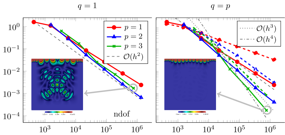
(a) Relative error.

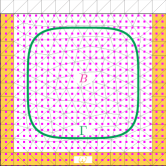
(b) Geometry.

Figure 3. Results for a Helmholtz problem using exact data. Solid and dashed lines show the relative $L^{2}$, respectively $H^{1}$-semi error, in the target domain $B$. In the insets the absolute error for the cases indicated by the arrows is shown.

We start by considering the case of exact data, i.e. $\delta=0$ in (24). The relative $L^{2}$-errors in the target domain under mesh refinement are shown in Figure 3(a). For $q=1$ the convergence for any polynomial degree $p$ is limited by the geometrical error, i.e. $\operatorname{dist}(\Gamma,\Gamma_{h})\lesssim\mathcal{O}(h^{2})$, introduced by the piecewise linear approximation of the interface. Interestingly the absolute error displayed in the inset of Figure 3(a) (left) looks like a spurious resonance and a strong pollution on part of the boundary where no data is given can be observed. When increasing the resolution of the geometry to $q=p$ (central plot in Figure 3) these effects are reduced significantly. We observe a convergence rate of $\mathcal{O}(h^{\tau q})$ in the $H^{1}$-semi norm with $\tau$ close to one and $\mathcal{O}(h^{\tau(q+1)})$ in the $L^{2}$-norm. This is better than predicted by our theoretical results, which in particular do not guarantee convergence in the $H^{1}$-semi norm at all. This is because the conditional stability estimate (5) merely yields control of the $L^{2}$-norm in the target domain. If such an estimate giving control over the $H^{1}$-norm was available, as e.g. derived in [11, Corollary 3] for the Helmholtz equation without interfaces in a specific convex geometric setting, then inspection of the proof of Theorem 4.5 shows that rates of $\mathcal{O}(h^{\tau q})$ in the $H^{1}$-norm would follow.

5.1.2. Perturbed data

Let us now consider perturbed data of strength $\delta=\tilde{\delta}_{p}h^{p-\theta}$ for some $\theta\in\{0,1,2\}$ and with $\tilde{\delta}_{p}$ independent of $h$. In the implementation these perturbations are realized by populating the degrees of freedom of a finite element function with random noise and subsequent normalization. Setting $q=p$ the error estimate of Theorem 4.5 predicts the following behavior:

$$\left\lVert u-u_{h}\circ\Phi_{h}^{-1}\right\rVert_{B}\lesssim h^{\tau p}\left(\left\lVert u\right\rVert_{p}+\tilde{\delta}_{p}h^{-\theta}\right).$$ (47)

Two different regimes can be distinguished:

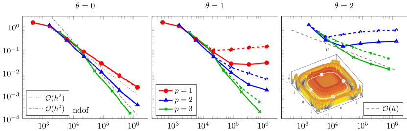
Figure 4. Results for a Helmholtz problem in a convex geometry using perturbed data with $\delta=\tilde{\delta}_{p}h^{p-\theta}$. Solid lines: $\tilde{\delta}_{p}\in[1,8,28]$ for $p\in[1,2,3]$, dashed line $\tilde{\delta}_{p}\in[5,24,80]$. All experiments use $q=p$.

• As long as $\left\lVert u\right\rVert_{p}h^{\theta}>\tilde{\delta}_{p}$ the first term in (47) will dominate. Then we expect to see the same convergence behavior as in Subsection 5.1.1 with exact data.

• When $h$ is small enough such that $\left\lVert u\right\rVert_{p}h^{\theta}<\tilde{\delta}_{p}$, then the second term takes over and the rate deteriorates to $\mathcal{O}(h^{\tau p-\theta})$.

The numerical results shown in Figure 4 confirm this behavior. The refinement level at which the transition from one regime to the other occurs can be shifted by scaling the coefficient $\tilde{\delta}_{p}$ of the noise as comparison of the solid and dashed lines in Figure 4 demonstrates.

5.2. Non-convex geometry in $d=2$

Let us now tackle a more challenging geometrical configuration sketched in Figure 5(b). The objective is to continue the solution given in $\omega=[-0.5,0.5]^{2}$ across the interface into $B=[-1.25,1.25]^{2}$. We will consider only exact data from now on.

5.2.1. Pure diffusion

Reconstructing the solution outside the convex hull of the data is very challenging for Helmholtz-type problems, see e.g. [11, 7, 15]. Therefore, we start by considering the purely diffusive problem first, i.e. $\rho_{i}=0$ for $i=1,2$. We use the reference solution

$$u=\begin{cases}\frac{1}{\sqrt{2}}\left(1+\pi\frac{\mu_{1}}{\mu_{2}}\right)-\cos\left(\frac{\pi\left\lVert x\right\rVert_{4}^{4}}{4}\right)&\text{ in }\Omega_{1},\\ \frac{\mu_{1}\pi}{\mu_{2}\sqrt{2}}\left\lVert x\right\rVert_{4}&\text{ in }\Omega_{2},\end{cases}$$ (48)

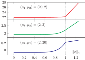
(a) Reference solution.

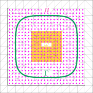
(b) Geometry.

Figure 5. Figure (a) shows the reference solution (48) in the purely diffusive case as a function of $\left\lVert x\right\rVert_{4}$ for different levels of the contrast. Figure (b) displays a sketch of the geometrical setup.

which is shown in Figure 5(a) as a function of $\left\lVert x\right\rVert_{4}$ for different levels of the contrast. Note that a kink occurs at the interface for $\mu_{1}\neq\mu_{2}$.

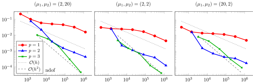
Figure 6. Dependence of the relative $L^{2}$-error in $B$ on the contrast for a pure diffusion problem in the non-convex geometry shown in Figure 5(b). Here we used $q=p$.

The relative $L^{2}$ errors in $B$ for different levels of the contrast are shown in Figure 6. This problem is slightly more challenging than the Helmholtz problem in the convex geometry as the rate does not exceed second order even for $p=3$. Nevertheless, we still obtain reasonably accurate solutions after a few refinement steps and the experiment even shows that contrasts of one order of magnitude in the diffusivities seem to be well-tolerated by the method. Here we have set the weights in the numerical flux to $\kappa_{1}=\mu_{2}/(\mu_{1}+\mu_{2})$ and $\kappa_{2}=\mu_{1}/(\mu_{1}+\mu_{2})$, which is a popular choice in the literature [22, 16, 23] for contrast problems.

As an additional experiment let us investigate the importance of the stabilization terms. In numerical experiments it is common practice to rescale these terms by some positive constants to optimize the preasymptotic convergence behavior. The stabilization terms $J_{\mathrm{CIP}}\left(\cdot,\cdot\right)$ and $J_{\mathrm{GLS}}\left(\cdot,\cdot\right)$ are a standard ingredient of methods based on the framework from [5]. Parameter studies on the optimal choice of the corresponding scaling parameters can be found in the literature, see e.g. [5, 10, 36, 15]. Here, we focus on the novel terms which appeared in this work, i.e. the choice of $\gamma_{\mathrm{IF}}$ for the interface stabilization in (28) and the choice of $\alpha_{2}$ in (29) which we introduced to counter propagation of geometric errors. The dependence of the relative $L^{2}$-error on the size of these parameters is displayed in Figure 7. This experiment has been carried out on the second finest mesh used for the previous convergence study. We discuss the results of the different stabilizations separately:

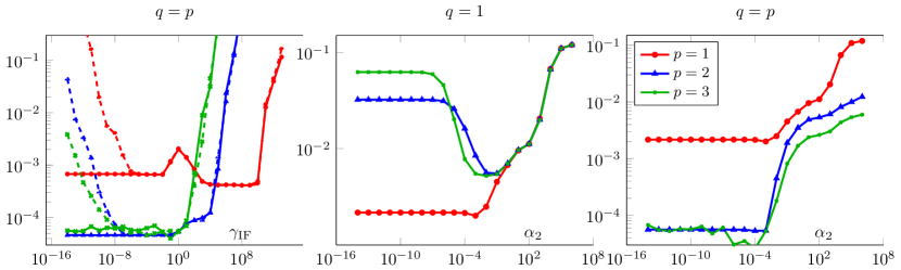
Figure 7. Dependence of the relative $L^{2}$-error in $B$ in terms of the choice of stabilization parameters. We consider a pure diffusion problem with $(\mu_{1},\mu_{2})=(20,2)$ in the non-convex geometry shown in Figure 5(b). The solid lines in the left plot show the results for the method as defined and analyzed in this paper, while dashed lines display the results for an alternative method in which the term $N_{h}^{c}$ in the bilinear form is omitted.

• The solid lines in the left plot of Figure 7 show that our method appears to be stable and accurate even when the stabilization on the interface is completely omitted, i.e.  $\gamma_{\mathrm{IF}}=0$. This is in fact due to the presence of the Nitsche term $N_{h}^{c}$ in the bilinear form $A_{h}$, see (22)-(23). If the latter term is omitted (dashed lines), the error increases dramatically as $\gamma_{\mathrm{IF}}$ goes to zero. Note that dropping $N_{h}^{c}$ means to sacrifice adjoint consistency of the Nitsche formulation, which seems to be of importance here.

• If the geometry is sufficiently resolved ($q=p$) it appears that $\alpha_{2}$ can be set to zero as well. This is reasonable since we introduced this stabilization to counter geometrical errors that are of order $\mathcal{O}(h^{q})$. However, when the geometry is underresolved (central plot with $q=1$) these geometric errors become significant and we indeed observe that the error in the target domain increases noticably when $\alpha_{2}$ is chosen too small and $p>1$. For $p=1$ on the other hand, we can always set $\alpha_{2}=0$ as the discrete Poincaré inequality given in [10, Lemma 2] ensures that the gradient weighted with $h$ is already controlled by the other stabilization terms.

5.2.2. Helmholtz problem

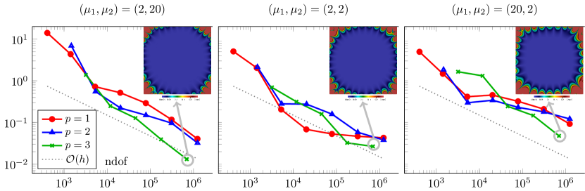
Figure 8. The relative $L^{2}$-error in $B$ for a Helmholz problem in a non-convex geometry. Here we have set $q=p$. In the insets the absolute error for the cases indicated by the arrows is shown.

Let us now consider the Helmholtz problem with $k_{1}=16,k_{2}=2$ in the non-convex geometry of Figure 5(b). The results for different contrasts are displayed in Figure 8. Clearly, the stability is very poor which results into slow convergence and makes the results difficult to interpret. Comparing the relative errors and pointwise absolute errors in the insets of the three plots suggests that having larger diffusion in the domain $\Omega_{2}$ is beneficial. This domain contains the bulk of the error which is concentrated near $\partial\Omega$. When the diffusion in this region is increased, which effectively decreases the wavenumber, the error seems to retreat slightly farther away from the target domain towards the boundary. These observations are consistent with similar results which were recently obtained for an elastodynamics problem in [15].

5.3. Convex geometry in $d=3$

Finally, we consider a three dimensional example similar to the setup from Subsection 5.1. Now the background domain is the cube $\Omega=[-1.75,1.75]^{3}$ and the objective is to extend the solution to $B=\Omega\setminus[-1.75,1.75]^{2}\times[1.2,1.75]$ where data is given in $\omega=B\setminus[-1.25,1.25]^{3}$. A sketch of the data domain is shown in the left part of Figure 9. Note that $B$ is the convex hull of $\omega$. We consider a purely diffusive problem using the reference solution (48) and $\mu_{1}=1,\mu_{2}=2$.

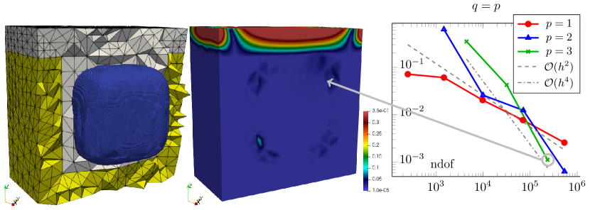
Figure 9. Left: data domain $\omega$ in yellow and subdomain $\Omega_{1}$ in blue. Middle: Absolute error on the finest mesh (shown on the left) considered for $p=3$. Right: Relative $L^{2}$-error in $B$.

The relative errors for $p=q$ are shown in Figure 9. Due to the high computational costs in three dimensions when using direct solvers we only performed a limited number of mesh refinements. The obtained results however indicate that the convergence rates appear to be similar as in the two-dimensional convex geometry considered in Subsection 5.1. This shows that our method is operational also in three dimensions, yet exposes the need to develop more efficients solvers for the linear systems to allow computations on finer meshes. The latter would also be required to solve Helmholtz problems at moderate to high frequencies.

6. Conclusion

We have investigated an unfitted FEM for unique continuation across an interface. To establish error estimates in the unfitted setting, we had to introduce additional stabilization terms on the interface and a weak Tikhonov penalization of the gradient in the bulk. The benefit of the latter has been observed in numerical experiments featuring geometrically underresolved regimes in which the distance between $\Gamma$ and $\Gamma_{h}$ is fairly large. At the analytical level we were able to understand the need for this particular stabilization by adopting a technique introduced in [28, 31] which allows for explicit control and analysis of geometric errors. It would be interesting to investigate whether our method and its analysis could be combined with other approaches for geometry approximation and numerical integration on unfitted geometries which have been proposed in the literature. In principle, any technique that can reduce the geometric error down to the level of the discretization error in a robust, accurate and (desirably) efficient way should be suitable.

Our numerical experiments suggest that the presence of a (smooth) interface itself seems to pose no major obstacle for the numerical solution of unique continuation problems for elliptic PDEs. Rather, the main challenge is to continue the solution beyond the convex hull of the data for problems of Helmholtz-type. However, this is already difficult if no interfaces are present [11, 7, 15]. Finally, we point out that our conclusions are naturally based on a fairly limited set of experiments and that further studies are necessary to reach definite conclusions. In particular, the influence of interfaces for ill-posed wave propagation problems in the time domain should be investigated in forthcoming research.

Appendix A Conditional stability estimate

From [20, Theorem 1.1] we get the following result: Let $u\in H^{1}(\Omega)$ be a solution of (1) where $f\in H^{-1}(\Omega)$ is of the form

$$\langle f,v\rangle=(f_{0},v)_{\Omega}+(F,\nabla v)_{\Omega}\text{ with }\left\lVert f_{0}\right\rVert_{\Omega}+\left\lVert F\right\rVert_{\Omega}\leqslant\varepsilon,$$ (49)

where we use the common notation $\langle\cdot,\cdot\rangle$ to denote the duality bracket on $H^{-1}\times H_{0}^{1}$. Then there exists $\bar{r}>0$ such that if $0<r_{1}<r_{2}<r_{3}<\bar{r}$, $x_{0}\in\Omega,\operatorname{dist}(x_{0},\partial\Omega)>r_{3}$, there exist $C>0,0<\tau<1$ such that

$$\left\lVert u\right\rVert_{B_{r_{2}}(x_{0})}\leqslant C\left(\left\lVert u\right\rVert_{B_{r_{1}}(x_{0})}+\varepsilon\right)^{\tau}\left(\left\lVert u\right\rVert_{B_{r_{3}}(x_{0})}+\varepsilon\right)^{1-\tau}.$$ (50)

Here, $B_{r_{j}}(x_{0})$ denotes the ball around $x_{0}$ with radius $r_{j},j=1,2,3$. We note that any $f\in H^{-1}(\Omega)$ with $\left\lVert f\right\rVert_{H^{-1}(\Omega)}\leqslant\varepsilon/2$ can be written in the form (49). Indeed, let $\phi\in H^{1}_{0}(\Omega)$ be the solution of the auxiliary problem

$$-\Delta\phi+\phi=f\in H^{-1}(\Omega).$$

Then clearly,

$$\langle f,v\rangle=(\phi,v)_{\Omega}+(\nabla\phi,\nabla v)_{\Omega}$$

for all $v\in H_{0}^{1}(\Omega)$. So we can take $f_{0}=\phi$ and $F=\nabla\phi$. Further,

$$\left\lVert f\right\rVert_{H^{-1}(\Omega)}=\sup_{v:\left\lVert v\right\rVert_{H^{1}(\Omega)=1}}\langle f,v\rangle=\sup_{v:\left\lVert v\right\rVert_{H^{1}(\Omega)=1}}(\phi,v)_{\Omega}+(\nabla\phi,\nabla v)_{\Omega}=\left\lVert\phi\right\rVert_{H^{1}(\Omega)}.$$

Hence,

$$\left\lVert f_{0}\right\rVert_{\Omega}+\left\lVert F\right\rVert_{\Omega}\leqslant 2\left\lVert\phi\right\rVert_{H^{1}(\Omega)}=2\left\lVert f\right\rVert_{H^{-1}(\Omega)}\leqslant\varepsilon.$$

Thus (50) yields

$$\left\lVert u\right\rVert_{B_{r_{2}}(x_{0})}\leqslant C\left(\left\lVert u\right\rVert_{B_{r_{1}}(x_{0})}+\left\lVert\mathcal{L}u\right\rVert_{H^{-1}(\Omega)}\right)^{\tau}\left(\left\lVert u\right\rVert_{B_{r_{3}}(x_{0})}+\left\lVert\mathcal{L}u\right\rVert_{H^{-1}(\Omega)}\right)^{1-\tau}.$$

The general case for $\omega\subset B\subset\Omega$ such that $B\setminus\omega$ does not touch the boundary stated in Corollary 1.2 then follows by using a covering argument, see [1, Section 5] or also [38].

Appendix B Proofs involving the isoparametric mapping

Lemma 13

1. From the construction of the mesh transformation, see [31, Section 3], we recall that

   $$\Psi-\Theta_{h}=\begin{cases}\Psi^{\Gamma}-\Theta_{h}^{\Gamma}&\text{ on }\Omega^{\Gamma},\\ E^{\partial\Omega^{\Gamma}}(\Psi^{\Gamma}-\Theta_{h}^{\Gamma})&\text{ on }\Omega^{\Gamma}_{+}\setminus\Omega^{\Gamma},\\ 0&\text{ on }\Omega\setminus\Omega^{\Gamma}_{+}.\end{cases}$$

   Here, $\Psi^{\Gamma}$ and $\Theta_{h}^{\Gamma}$ are local mappings on the cut elements $\Omega^{\Gamma}$ which are extended to a slightly larger domain $\Omega^{\Gamma}_{+}$ by a certain extension operator $E^{\partial\Omega^{\Gamma}}$, which according to [31, Theorem 3.11] fulfills

   $$\max_{T\in\mathcal{T}^{\Gamma}_{+}\setminus\mathcal{T}^{\Gamma}}\left\lVert D^{n}E^{\partial\Omega^{\Gamma}}w\right\rVert_{\infty,T}\lesssim\max_{F\in\mathcal{F}(\partial\Omega^{\Gamma})}\sum\limits_{r=n}^{q+1}h^{r-n}\left\lVert D^{r}w\right\rVert_{\infty,F},\quad n=2,\ldots,q+1.$$ (51)

   Here, $\mathcal{F}(\partial\Omega^{\Gamma})$ denotes the set of all edges ($d=2$) or faces ($d=3$) in $\partial\Omega^{\Gamma}$ and $\mathcal{T}^{\Gamma}_{+}\setminus\mathcal{T}^{\Gamma}$ the set of elements convering the extended region $\Omega^{\Gamma}_{+}\setminus\Omega^{\Gamma}$. We also have from [31, Lemma 3.7] the estimate

   $$\sum\limits_{r=0}^{q+1}h^{r}\max_{T\in\mathcal{T}^{\Gamma}}\left\lVert D^{r}(\Psi^{\Gamma}-\Theta_{h}^{\Gamma})\right\rVert_{\infty,T}\lesssim h^{q+1}$$ (52)

   which already proves the claim (a) on $\Omega^{\Gamma}$. It remains to consider

   $$\max_{T\in\mathcal{T}^{\Gamma}_{+}\setminus\mathcal{T}^{\Gamma}}\left\lVert D^{l}E^{\partial\Omega^{\Gamma}}(\Psi^{\Gamma}-\Theta_{h}^{\Gamma})\right\rVert\lesssim\max_{F\in\mathcal{F}(\partial\Omega^{\Gamma})}\sum\limits_{r=l}^{q+1}h^{r-l}\left\lVert D^{r}(\Psi^{\Gamma}-\Theta_{h}^{\Gamma})\right\rVert_{\infty,F}$$

   $$\lesssim h^{-l}\max_{T\in\mathcal{T}^{\Gamma}}\sum\limits_{r=0}^{q+1}h^{r}\left\lVert D^{r}(\Psi^{\Gamma}-\Theta_{h}^{\Gamma})\right\rVert_{\infty,T}\lesssim h^{q+1-l}.$$

   where (51) and (52) have been employed. For passing from the facet to the element we also used that the involved functions are continuous on the elements so that the $L^{\infty}$-norm coincides with the supremum norm, see e.g. [24, Chapter 6.1].

2. Recall that $\Phi-\mathrm{id}=(\Psi-\Theta_{h})\Theta_{h}^{-1}$. In [29, Lemma 2] the bounds

   $$\left\lVert D^{l}\Theta_{h}^{-1}\right\rVert_{\infty,\Theta_{h}(T)}\lesssim 1,\quad\text{ for }l\in\{1,\ldots,q+1\}$$

   have been shown (for $l\in\{0,1\}$ the bounds actually hold globally, see proof of [31, Lemma 5.5.]). Hence, in view of part (a) the claim follows from the product rule.

Lemma 14 We will only prove the results on $\Gamma$ as the statements on $\Gamma_{h}$ follow analogously.

1. From the reverse triangle inequality we obtain for $x\in\Gamma$

   $$\left\lvert\left\lVert\underline{A}^{T}(x)n_{\Gamma}(x)\right\rVert_{2}-1\right\rvert=\left\lvert\left\lVert\underline{A}^{T}(x)n_{\Gamma}(x)\right\rVert_{2}-\left\lVert n_{\Gamma}(x)\right\rVert_{2}\right\rvert\leqslant\left\lVert(\underline{A}^{T}(x)-I)n_{\Gamma}(x)\right\rVert_{2}.$$

   Since $\Theta_{h}(\mathcal{T}_{h})$ covers $\Omega$, there exists an element $T$ such that $x\in\Theta_{h}(T)$. As $\underline{A}^{T}$ is continuous on $\Theta_{h}(T)$ we obtain:

   $$\left\lVert(\underline{A}^{T}(x)-I)n_{\Gamma}(x)\right\rVert_{2}\lesssim\left\lVert\underline{A}^{T}-I\right\rVert_{\infty,\Theta_{h}(T)}\lesssim h^{q},$$

   where (12) was used in the last step. As a result, the lower bound

   $$\left\lVert\underline{A}^{T}n_{\Gamma}\right\rVert_{2}\geqslant 1-\left\lvert\left\lVert\underline{A}^{T}n_{\Gamma}\right\rVert_{2}-1\right\rvert\gtrsim 1$$

   for $h$ sufficiently small follows.

2. Using (14), (12) and (a) we obtain

   $$\left\lVert n_{\Gamma}-n_{\Gamma_{h}}\circ\Phi_{h}^{-1}\right\rVert_{2}=\frac{1}{\left\lVert\underline{A}^{T}n_{\Gamma}\right\rVert_{2}}\left\lVert n_{\Gamma}\left\lVert\underline{A}^{T}n_{\Gamma}\right\rVert-\underline{A}^{T}n_{\Gamma}\right\rVert_{2}$$

   $$\lesssim\left\lVert n_{\Gamma}\left(\left\lVert\underline{A}^{T}n_{\Gamma}\right\rVert_{2}-1\right)+\left(I-\underline{A}^{T}\right)n_{\Gamma}\right\rVert_{2}\lesssim\left\lvert\left\lVert\underline{A}^{T}n_{\Gamma}\right\rVert_{2}-1\right\rvert+\left\lVert I-\underline{A}^{T}\right\rVert_{2}\lesssim h^{q}.$$

3. From the result established in (b) we obtain

   $$\left\lVert P_{\Gamma_{h}}\circ\Phi_{h}^{-1}-P_{\Gamma}\right\rVert_{2} =\left\lVert(n_{\Gamma_{h}}\circ\Phi_{h}^{-1}-n_{\Gamma})(n_{\Gamma_{h}}\circ\Phi_{h}^{-1})^{T}+n_{\Gamma}(n_{\Gamma_{h}}\circ\Phi_{h}^{-1}-n_{\Gamma})^{T}\right\rVert_{2}$$

   $$\lesssim\left\lVert n_{\Gamma_{h}}\circ\Phi_{h}^{-1}-n_{\Gamma}\right\rVert_{2}+\left\lVert(n_{\Gamma_{h}}\circ\Phi_{h}^{-1}-n_{\Gamma})^{T}\right\rVert_{2}\lesssim h^{q}.$$

Lemma 2.5

1. See [31, proof of Lemma 5.10].

2. According to the chain rule

   $$\partial_{y_{\nu}}\partial_{y_{\mu}}\tilde{v}(y) =\sum\limits_{j=1}^{d}\sum\limits_{k=1}^{d}(\partial_{j}\partial_{k}v)\circ\Phi_{h}(y)\partial_{y_{\nu}}[\Phi_{h}]_{j}(y)\partial_{y_{\mu}}[\Phi_{h}]_{k}(y)$$

   $$+\sum\limits_{k=1}^{d}(\partial_{k}v)\circ\Phi_{h}(y)\partial_{y_{\nu}}\partial_{y_{\mu}}[\Phi_{h}]_{k}(y),$$

   where $[\Phi_{h}]_{j},j=1,\ldots,d$ denote the components of $\Phi_{h}$. In view of $\Theta_{h}=\Phi_{h}^{-1}\circ\Psi$ the transformation formula for integrals yields

   $$\sum\limits_{T\in\mathcal{T}_{h}^{i}}\int\limits_{\Theta_{h}(T)}\left\lvert\partial_{y_{\nu}}\partial_{y_{\mu}}\tilde{v}\right\rvert^{2}\;\mathrm{d}y=\sum\limits_{T\in\mathcal{T}_{h}^{i}}\int\limits_{\Psi(T)}\left\lvert(\partial_{y_{\nu}}\partial_{y_{\mu}}\tilde{v})\circ\Phi_{h}^{-1}(x)\right\rvert^{2}\det(\underline{A}^{-1}(x))\;\mathrm{d}x$$

   $$\lesssim\sum\limits_{T\in\mathcal{T}_{h}^{i}}\sum\limits_{j,k}\int\limits_{\Psi(T)}\left\lvert(\partial_{j}\partial_{k}v(x)\right\rvert^{2}\left\lvert\partial_{\nu}[\Phi_{h}]_{j}(\Phi_{h}^{-1}(x))\partial_{\mu}[\Phi_{h}]_{k}(\Phi_{h}^{-1}(x))\right\rvert^{2}\;\mathrm{d}x$$

   $$+\sum\limits_{T\in\mathcal{T}_{h}^{i}}\sum\limits_{k=1}^{d}\int\limits_{\Psi(T)}\left\lvert\partial_{k}v(x)\right\rvert^{2}\left\lvert\partial_{\nu}\partial_{\mu}[\Phi_{h}]_{k}(\Phi_{h}^{-1}(x))\right\rvert^{2}\;\mathrm{d}x$$

   $$\lesssim\sum\limits_{\left\lvert\alpha\right\rvert\leqslant 2}\sum\limits_{T\in\mathcal{T}_{h}^{i}}\int\limits_{\Psi(T)}\left\lvert D_{x}^{\alpha}v\right\rvert^{2}\;\mathrm{d}x,$$

   where we applied the bounds for the second derivatives from Lemma 13 (b) on $\Phi_{h}^{-1}\circ\Psi(T)=\Theta_{h}(T)$ and (13).

Lemma 2.5 We recall from [31, eq. (3.40)] that the measures $\mathrm{d}S_{\Gamma}$ on $\Gamma$ and $\mathrm{d}S_{\Gamma_{h}}$ on $\Gamma_{h}$ are related as follows:

$$\mathrm{d}S_{\Gamma}=\det(\underline{A})\left\lVert\underline{A}^{-T}n_{\Gamma_{h}}\right\rVert_{2}\mathrm{d}S_{\Gamma_{h}},\quad\mathrm{d}S_{\Gamma_{h}}=\det(\underline{A}^{-1})\left\lVert\underline{A}^{T}n_{\Gamma}\right\rVert_{2}\mathrm{d}S_{\Gamma}.$$ (53)

1. We will only show the result for the gradient. Using $(\nabla v)\circ\Phi_{h}=\underline{A}^{-T}\nabla\tilde{v}$ and the transformation rule (53) for the measure yields

   $$\int\limits_{\Gamma}\left\lvert\nabla v\right\rvert^{2}\mathrm{d}S_{\Gamma} =\int\limits_{\Gamma_{h}}\left\lvert\underline{A}^{-T}\nabla\tilde{v}\right\rvert^{2}\det(\underline{A})\left\lVert\underline{A}^{-T}n_{\Gamma_{h}}\right\rVert_{2}\mathrm{d}S_{\Gamma_{h}}\lesssim\int\limits_{\Gamma_{h}}\left\lvert\nabla\tilde{v}\right\rvert^{2}\mathrm{d}S_{\Gamma_{h}},$$

   where the last inequality follows from equation (13). The reverse estimate is obtained in the same way by transforming from $\Gamma_{h}$ to $\Gamma$ and appealing to equations (12)-(13). The situation is similar in (b) and (c) where we will likewise only show one of the directions.

2. Using $\underline{A}^{T}\nabla v=(\nabla\tilde{v})\circ\Phi_{h}^{-1}$ and the transformation rule (53) gives

   $$\int\limits_{\Gamma_{h}}\left\lVert\nabla\tilde{v}\cdot n_{\Gamma_{h}}\right\rVert_{2}^{2}\mathrm{d}S_{\Gamma_{h}}=\int\limits_{\Gamma}\left\lVert\underline{A}^{T}\nabla v\cdot(n_{\Gamma_{h}}\circ\Phi_{h}^{-1})\right\rVert_{2}^{2}\det(\underline{A}^{-1})\left\lVert\underline{A}^{T}n_{\Gamma}\right\rVert_{2}\mathrm{d}S_{\Gamma}$$

   $$\lesssim \int\limits_{\Gamma}\left[\left\lVert\underline{A}^{T}\nabla v\cdot(n_{\Gamma_{h}}\circ\Phi_{h}^{-1}-n_{\Gamma})\right\rVert_{2}+\left\lVert(\underline{A}^{T}-I)\nabla v\cdot n_{\Gamma}\right\rVert_{2}\right]^{2}\left\lvert\det(\underline{A}^{-1})\right\rvert\left\lVert\underline{A}^{T}n_{\Gamma}\right\rVert_{2}\mathrm{d}S_{\Gamma}$$

   $$+\int\limits_{\Gamma}\left\lVert\nabla v\cdot n_{\Gamma}\right\rVert_{2}^{2}\left\lvert\det(\underline{A}^{-1})\right\rvert\left\lVert\underline{A}^{T}n_{\Gamma}\right\rVert_{2}\mathrm{d}S_{\Gamma}$$

   $$\lesssim h^{2q}\left\lVert\nabla v\right\rVert_{\Gamma}^{2}+\left\lVert\nabla v\cdot n_{\Gamma}\right\rVert_{\Gamma}^{2},$$

   where Lemma 14 (b), equation (12) and (13) were employed in the last step.

3. Writing $P_{\Gamma_{h}}\circ\Phi_{h}^{-1}\underline{A}^{T}=P_{\Gamma_{h}}\circ\Phi_{h}^{-1}(\underline{A}^{T}-I)+(P_{\Gamma_{h}}\circ\Phi_{h}^{-1}-P_{\Gamma})+P_{\Gamma}$ we deduce the claim from Lemma 14 (c), equation (12) and (13):

   $$\int\limits_{\Gamma_{h}}\left\lVert\nabla_{\Gamma_{h}}\tilde{v}\right\rVert_{2}^{2}\mathrm{d}S_{\Gamma}=\int\limits_{\Gamma}\left\lVert P_{\Gamma_{h}}\circ\Phi_{h}^{-1}\underline{A}^{T}\nabla v\right\rVert_{2}^{2}\det(\underline{A}^{-1})\left\lVert\underline{A}^{T}n_{\Gamma}\right\rVert_{2}\mathrm{d}S_{\Gamma}$$

   $$\lesssim\int\limits_{\Gamma}\left[\left\lVert P_{\Gamma_{h}}\circ\Phi_{h}^{-1}(\underline{A}^{T}-I)\nabla v\right\rVert_{2}+\left\lVert(P_{\Gamma_{h}}\circ\Phi_{h}^{-1}-P_{\Gamma})\nabla v\right\rVert_{2}\right]^{2}\left\lvert\det(\underline{A}^{-1})\right\rvert\left\lVert\underline{A}^{T}n_{\Gamma}\right\rVert_{2}\mathrm{d}S_{\Gamma}$$

   $$+\int\limits_{\Gamma}\left\lVert P_{\Gamma}\nabla v\right\rVert_{2}^{2}\left\lvert\det(\underline{A}^{-1})\right\rvert\left\lVert\underline{A}^{T}n_{\Gamma}\right\rVert_{2}\mathrm{d}S_{\Gamma}$$

   $$\lesssim h^{2q}\left\lVert\nabla v\right\rVert_{\Gamma}^{2}+\left\lVert\nabla_{\Gamma}v\right\rVert_{\Gamma}^{2}.$$

Lemma 2.5

1. Let $\gamma(s):=f(s\Phi_{h}^{-1}(x)+(1-s)x)$ for $s\in[0,1]$ and $x\in M$. We have

   $$f\circ\Phi_{h}^{-1}(x)-f(x)=\int\limits_{0}^{1}\gamma^{\prime}(s)\mathrm{d}s =\int\limits_{0}^{1}(\nabla f(s\Phi_{h}^{-1}(x)+(1-s)x),\Phi_{h}^{-1}(x)-x)\;\mathrm{d}s$$

   $$\lesssim\left\lVert\nabla f\right\rVert_{\infty,U}\left\lVert\Phi_{h}^{-1}(x)-x\right\rVert_{2}.$$

   Hence, we obtain from Lemma 2.4 that

   $$\left\lVert f\circ\Phi_{h}^{-1}-f\right\rVert_{M}\lesssim\sqrt{\left\lvert M\right\rvert}\left\lVert\nabla f\right\rVert_{\infty,U}\left\lVert\Phi_{h}^{-1}-\mathrm{id}\right\rVert_{\infty,\Omega}\lesssim h^{q+1}\sqrt{\left\lvert M\right\rvert}\left\lVert\nabla f\right\rVert_{\infty,U}.$$

2. We have

   $$\left\lVert\nabla(f\circ\Phi_{h}^{-1}-f)\right\rVert_{M}=\left\lVert\underline{A}^{-T}\nabla f\circ\Phi_{h}^{-1}-\nabla f\right\rVert_{M}$$

   $$\lesssim\left\lVert(\underline{A}^{-T}-I)[(\nabla f\circ\Phi_{h}^{-1}-\nabla f)+\nabla f]+(\nabla f\circ\Phi_{h}^{-1}-\nabla f)\right\rVert_{M}$$

   $$\lesssim\left(\left\lVert\underline{A}^{-T}-I\right\rVert_{\infty,M}+1\right)\left\lVert\nabla f\circ\Phi_{h}^{-1}-\nabla f\right\rVert_{M}+\left\lVert\underline{A}^{-T}-I\right\rVert_{\infty,M}\left\lVert\nabla{f}\right\rVert_{M}$$

   $$\lesssim h^{q+1}\sqrt{\left\lvert M\right\rvert}\left\lVert f\right\rVert_{W^{2,\infty}(U)}+h^{q}\left\lVert\nabla f\right\rVert_{M},$$

   where part (a) was employed to estimate the first term and we used (13) to obtain the bound for the second term.

3. By the chain rule we have

   $$\partial_{x_{\nu}}\partial_{x_{\mu}}(f\circ\Phi_{h})=(\partial_{\nu}\partial_{\mu}f)\circ\Phi_{h}+(\partial_{\nu}\partial_{\mu}f)\circ\Phi_{h}(\partial_{x_{\mu}}[\Phi_{h}]_{\mu}-1)$$

   $$(\partial_{\nu}\partial_{\mu}f)\circ\Phi_{h}(\partial_{x_{\nu}}[\Phi_{h}]_{\nu}-1)\partial_{x_{\mu}}[\Phi_{h}]_{\mu}+\sum\limits_{(i,j)\neq(\mu,\nu)}(\partial_{j}\partial_{i}f)\circ\Phi_{h}\partial_{x_{\nu}}[\Phi_{h}]_{j}\partial_{x_{\mu}}[\Phi_{h}]_{i}$$

   $$+\sum\limits_{i}(\partial_{i}f)\circ\Phi_{h}\partial_{x_{\nu}}\partial_{x_{\mu}}[\Phi_{h}]_{i},$$ (54)

   where $[\Phi_{h}]_{i}$ denotes the $i$-th component of $\Phi_{h}$. According to Lemma 2.4 we have

   $$\left\lVert\partial_{x_{j}}[\Phi_{h}]_{i}\right\rVert_{\infty,\Omega}\lesssim h^{q}\text{ for }i\neq j,\quad\left\lVert\partial_{x_{j}}[\Phi_{h}]_{j}-1\right\rVert_{\infty,\Omega}\lesssim h^{q}\text{ for }j=1,\ldots,d.$$

   Combining this with the bounds for the second derivatives from Lemma 13 on $M=\Theta_{h}(T)$ yields

   $$\left\lVert\partial_{x_{\nu}}\partial_{x_{\mu}}(f\circ\Phi_{h})-\partial_{x_{\nu}}\partial_{x_{\mu}}f\right\rVert_{M}$$

   $$\lesssim\left\lVert(\partial_{x_{\nu}}\partial_{x_{\mu}}f)\circ\Phi_{h}-\partial_{x_{\nu}}\partial_{x_{\mu}}f\right\rVert_{M}+\sqrt{\left\lvert M\right\rvert}\left(h^{q}\left\lVert f\right\rVert_{W^{2,\infty}(V)}+h^{q-1}\left\lVert f\right\rVert_{W^{1,\infty}(V)}\right)$$

   $$\lesssim h^{q-1}\sqrt{\left\lvert M\right\rvert}\left\lVert f\right\rVert_{W^{3,\infty}(V)},$$

   where part (a) was once again applied in the last step.

4. If we precompose equation (54) with $\Phi_{h}^{-1}$ we obtain

   $$\partial_{x_{\nu}}\partial_{x_{\mu}}(f\circ\Phi_{h})\circ\Phi_{h}^{-1}-\partial_{x_{\nu}}\partial_{x_{\mu}}f=(\partial_{\nu}\partial_{\mu}f)(\partial_{x_{\nu}}[\Phi_{h}]_{\nu}\circ\Phi_{h}^{-1}-1)\partial_{x_{\mu}}[\Phi_{h}]_{\mu}\circ\Phi_{h}^{-1}$$

   $$+(\partial_{\nu}\partial_{\mu}f)(\partial_{x_{\mu}}[\Phi_{h}]_{\mu}\circ\Phi_{h}^{-1}-1)+\sum\limits_{(i,j)\neq(\mu,\nu)}(\partial_{j}\partial_{i}f)\partial_{x_{\nu}}[\Phi_{h}]_{j}\circ\Phi_{h}^{-1}\partial_{x_{\mu}}[\Phi_{h}]_{i}\circ\Phi_{h}^{-1}$$

   $$+\sum\limits_{i}(\partial_{i}f)\partial_{x_{\nu}}\partial_{x_{\mu}}[\Phi_{h}]_{i}\circ\Phi_{h}^{-1}.$$

   Since the term $\partial_{x_{\nu}}\partial_{x_{\mu}}f$ is now on the left hand side of the equation, it is no longer necessary to appeal to part (a) to estimate this term. We can directly apply Lemma 2.4 to estimate the first order derivatives of $\Phi_{h}$ and Lemma 13 to obtain bounds for the second order derivatives on $\Phi_{h}^{-1}\circ\Psi(T)=\Theta_{h}(T)$. Hence,

   $$\left\lVert\partial_{x_{\nu}}\partial_{x_{\mu}}(f\circ\Phi_{h})\circ\Phi_{h}^{-1}-\partial_{x_{\nu}}\partial_{x_{\mu}}f\right\rVert_{\Psi(T)}\lesssim h^{q}\left\lVert f\right\rVert_{H^{2}(\Psi(T))}+h^{q-1}\left\lVert\nabla f\right\rVert_{\Psi(T)}$$

   follows.

References

- [1] Giovanni Alessandrini, Luca Rondi, Edi Rosset, and Sergio Vessella. The stability for the Cauchy problem for elliptic equations. Inverse Probl., 25(12):123004, nov 2009.
- [2] Christine Bernardi. Optimal Finite-Element Interpolation on Curved Domains. SIAM J. Numer. Anal., 26(5):1212–1240, 1989.
- [3] Thomas Boiveau, Erik Burman, Susanne Claus, and Mats Larson. Fictitious domain method with boundary value correction using penalty-free Nitsche method. J. Numer. Math., 26(2):77–95, 2018.
- [4] Muriel Boulakia, Erik Burman, Miguel A. Fernández, and Colette Voisembert. Data assimilation finite element method for the linearized Navier–Stokes equations in the low Reynolds regime. Inverse Probl., 36(8):085003, aug 2020.
- [5] Erik Burman. Stabilized Finite Element Methods for Nonsymmetric, Noncoercive, and Ill-Posed Problems. Part I: Elliptic Equations. SIAM J. Sci. Comput., 35(6):A2752–A2780, 2013.
- [6] Erik Burman, Susanne Claus, Peter Hansbo, Mats G Larson, and André Massing. CutFEM: discretizing geometry and partial differential equations. Int. J. Numer. Methods Eng., 104(7):472–501, 2015.
- [7] Erik Burman, Guillaume Delay, and Alexandre Ern. A Hybridized High-Order Method for Unique Continuation Subject to the Helmholtz Equation. SIAM J. Numer. Anal., 59(5):2368–2392, 2021.
- [8] Erik Burman and Alexandre Ern. An Unfitted Hybrid High-Order Method for Elliptic Interface Problems. SIAM J. Numer. Anal., 56(3):1525–1546, 2018.
- [9] Erik Burman, Peter Hansbo, and Mats Larson. A cut finite element method with boundary value correction. Math. Comput., 87(310):633–657, 2018.
- [10] Erik Burman, Peter Hansbo, and Mats G Larson. Solving ill-posed control problems by stabilized finite element methods: an alternative to Tikhonov regularization. Inverse Probl., 34(3):035004, jan 2018.
- [11] Erik Burman, Mihai Nechita, and Lauri Oksanen. Unique continuation for the Helmholtz equation using stabilized finite element methods. J. Math. Pures Appl., 129:1–22, 2019.
- [12] Erik Burman, Mihai Nechita, and Lauri Oksanen. A stabilized finite element method for inverse problems subject to the convection–diffusion equation. I: diffusion-dominated regime. Numer. Math., 144(3):451–477, 2020.
- [13] Erik Burman, Mihai Nechita, and Lauri Oksanen. A stabilized finite element method for inverse problems subject to the convection–diffusion equation. II: convection-dominated regime. Numer. Math., 150(3):769–801, 2022.
- [14] Erik Burman and Janosch Preuss. Reproduction material: Unique continuation for an elliptic interface problem using unfitted isoparametric finite elements, July 2023.
- [15] Erik Burman and Janosch Preuss. Unique continuation for the Lamé system using stabilized finite element methods. GEM - Int. J. Geomath., 14(1):9, 2023.
- [16] Erik Burman and Paolo Zunino. A Domain Decomposition Method Based on Weighted Interior Penalties for Advection‐Diffusion‐Reaction Problems. SIAM J. Numer. Anal., 44(4):1612–1638, 2006.
- [17] Burman, Erik, Feizmohammadi, Ali, Münch, Arnaud, and Oksanen, Lauri. Space time stabilized finite element methods for a unique continuation problem subject to the wave equation. ESAIM: M2AN, 55:S969–S991, 2021.
- [18] Burman, Erik, Feizmohammadi, Ali, Münch, Arnaud, and Oksanen, Lauri. Spacetime finite element methods for control problems subject to the wave equation. ESAIM: COCV, 29:41, 2023.
- [19] Zhiming Chen, Ke Li, and Xueshuang Xiang. An adaptive high-order unfitted finite element method for elliptic interface problems. Numer. Math., 149(3):507–548, 2021.
- [20] Cătălin I. Cârstea and Jenn-Nan Wang. Propagation of smallness for an elliptic PDE with piecewise Lipschitz coefficients. J. Differ. Equ., 268(12):7609–7628, 2020.
- [21] Wolfgang Dahmen, Harald Monsuur, and Rob Stevenson. Least squares solvers for ill-posed PDEs that are conditionally stable. ESAIM: M2AN, 57(4):2227–2255, 2023.
- [22] Maksymilian Dryja. On Discontinuous Galerkin Methods for Elliptic Problems with Discontinuous Coefficients. Comput. Methods Appl. Math., 3(1):76–85, 2003.
- [23] Alexandre Ern, Annette F. Stephansen, and Paolo Zunino. A discontinuous Galerkin method with weighted averages for advection–diffusion equations with locally small and anisotropic diffusivity. IMA J. Numer. Anal., 29(2):235–256, 2009.
- [24] Gerald B Folland. Real analysis: modern techniques and their applications. Pure and Applied Mathematics. John Wiley & Sons, New York, 2nd edition, 1999.
- [25] Roland Glowinski, Chin-Hsien Li, and Jacques-Louis Lions. A numerical approach to the exact boundary controllability of the wave equation (I) Dirichlet controls: Description of the numerical methods. Japan J. Appl. Math., 7:1–76, 1990.
- [26] Jörg Grande, Christoph Lehrenfeld, and Arnold Reusken. Analysis of a high-order trace finite element method for pdes on level set surfaces. SIAM J. Numer. Anal., 56(1):228–255, 2018.
- [27] Anita Hansbo and Peter Hansbo. An unfitted finite element method, based on Nitsche’s method, for elliptic interface problems. Comput. Methods Appl. Mech. Engrg., 191(47-48):5537–5552, 2002.
- [28] Christoph Lehrenfeld. High order unfitted finite element methods on level set domains using isoparametric mappings. Comput. Methods Appl. Mech. Eng., 300:716 – 733, 2016.
- [29] Christoph Lehrenfeld. A higher order isoparametric fictitious domain method for level set domains. In Stéphane P. A. Bordas, Erik Burman, Mats G. Larson, and Maxim A. Olshanskii, editors, Geometrically Unfitted Finite Element Methods and Applications, pages 65–92. Springer International Publishing, Cham, 2017.
- [30] Christoph Lehrenfeld, Fabian Heimann, Janosch Preuß, and Henry von Wahl. ngsxfem: Add-on to NGSolve for geometrically unfitted finite element discretizations. J. Open Source Softw., 6(64):3237, 2021.
- [31] Christoph Lehrenfeld and Arnold Reusken. Analysis of a high order unfitted finite element method for an elliptic interface problem. IMA J. Numer. Anal., 00:1–37, 2017. first online.
- [32] Christoph Lehrenfeld and Arnold Reusken. -estimates for a high order unfitted finite element method for elliptic interface problems. J. Numer. Math., 00:–, 2018.
- [33] Yimin Lou. High-order Unfitted Discretizations for Partial Differential Equations Coupled with Geometric Flow. PhD thesis, University of Göttingen, February 2023.
- [34] Ralf Massjung. An Unfitted Discontinuous Galerkin Method Applied to Elliptic Interface Problems. SIAM J. Numer. Anal., 50(6):3134–3162, 2012.
- [35] Siddhartha Mishra and Roberto Molinaro. Estimates on the generalization error of physics-informed neural networks for approximating PDEs. IMA J. Numer. Anal., 43(1):1–43, 01 2022.
- [36] Mihai Nechita. Unique continuation problems and stabilised finite element methods. PhD thesis, University College London, 10 2020.
- [37] Arnold Reusken. Analysis of an extended pressure finite element space for two-phase incompressible flows. Comput. Vis. Sci., 11(4):293–305, 2008.
- [38] Luc Robbiano. Théorème d’unicité adapté au contrôle des solutions des problèmes hyperboliques. Commun. Partial Differ. Equ., 16(4-5):789–800, 1991.
- [39] Joachim Schöberl. NETGEN An advancing front 2D/3D-mesh generator based on abstract rules. Comput. Vis. Sci., 1(1):41–52, 1997.
- [40] Joachim Schöberl. C++11 implementation of finite elements in NGSolve. Technical report, ASC-2014-30, Institute for Analysis and Scientific Computing, September 2014.
- [41] Elias M. Stein. Singular Integrals and Differentiability Properties of Functions (PMS-30), Volume 30. Princeton University Press, Princeton, 1971.
- [42] Haijun Wu and Yuanming Xiao. An unfitted -Interface Penalty Finite Element Method for Elliptic Interface Problems. J. Comput. Math., 37(3):316–339, 2018.
- [43] Yuanming Xiao, Jinchao Xu, and Fei Wang. High-order extended finite element methods for solving interface problems. Comput. Methods Appl. Mech. Eng., 364:112964, 2020.
- [44] Paolo Zunino, Laura Cattaneo, and Claudia Maria Colciago. An unfitted interface penalty method for the numerical approximation of contrast problems. Appl. Numer. Math., 61(10):1059–1076, 2011.