Direct sampling of short paths for contiguous partitioning

Abstract

In this paper, we provide a family of dynamic programming based algorithms to sample nearly-shortest self avoiding walks between two points of the integer lattice $\mathbb{Z}^{2}$. We show that if the shortest path of between two points has length $n$, then we can sample paths (self-avoiding-walks) of length $n+O(n^{1-\delta)})$ in polynomial time. As an example of an application, we will show that the Glauber dynamics Markov chain for partitions of the Aztec Diamonds in $\mathbb{Z}^{2}$ into two contiguous regions with nearly tight perimeter constraints has exponential mixing time, while the algorithm provided in this paper can be used be used to uniformly (and exactly) sample such partitions efficiently.

1 Introduction

Analysis of political redistrictings has created a significant impetus for the problem of random sampling of graph partitions into connected pieces—e.g., into districtings.

The most common approach to this problem in practice is to use a Markov Chain; e.g., Glauber dynamics, or chains based on cutting spanning trees (e.g., DeFord et al. (2019); Autrey et al. (2019b); Autry et al. (2021)). Rigorous understanding of mixing behavior is the exception rather than the rule; for example, Montanari and Penna (2015a) established rapid mixing of a Markov chain for the special case where both partition classes are unions of horizontal bars, which in each case meet a common side. No rigorous approach is known, for example, which can approximately uniformly sample from contiguous $2$-partitions even of lattice graphs like the $n\times n$ grid in polynomial time

In this paper we consider a direct approach, where instead of leveraging a Markov chain with unknown mixing time to generate approximate uniform samples, we use a dynamic programming algorithm and rejection sampling to exactly sample from self-avoiding walks in the lattice $\mathbb{Z}^{2}$ (which correspond to partition boundaries) in polynomial expected time. Counting self-avoiding lattice walks is a significant long-standing challenge; the connective constant—the base of the exponent in the asymptotic formula for the number of such walks—is not even known for $\mathbb{Z}^{2}$. But we will be interested in sampling nearly-shortest self avoiding walks, motivated by districting constraints which discourage the use of large district perimeters relative to area. In particular, we will prove:

Theorem 1

For any $C$ and $\varepsilon>0$ and for any $n_{1},n_{2},$ and $n=n_{1}+n_{2}$, there is a randomized algorithm which runs w.h.p in polynomial time, and produces a uniform sample from the set of self-avoiding walks in $\mathbb{Z}^{2}$ from $(0,0)$ to $(n_{1},n_{2})$ of length at most

$$n+Cn^{1-\varepsilon}.$$

Figure 1: Uniformly random self-avoiding walks of length 700 between corners of a $300\times 300$ grid, generated with the algorithm from Theorem 1.

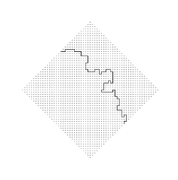
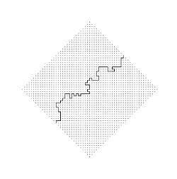
Figure 2: Uniformly random self-avoiding walks on $A_{30}$ such that both sides have perimeter of at most $220$.

A variant of this algorithm can be used to sample from contiguous $2$-partitions of the Aztec diamond with restricted partition-class perimeter, by sampling short paths between nearly-antipodal points on the dual of the Aztec diamond. These paths are in bijection with the contiguous $2$-partitions of the Aztec diamond, by mapping a partition to it’s boundary which gives us a path. This approach generates samples in polynomial time w.h.p. In contrast, we show that the traditional approach using Markov chains is inefficient:

Theorem 2

For any $C$ and $\varepsilon>0$, Glauber dynamics has exponential mixing time on contiguous $2$-partitions of the Aztec diamond $A_{k}$ when constrained by perimeter slack $Ck^{1-\varepsilon}$.

Organization of the Paper: The paper is organized in the following manner: Section 2 describes a dynamic programming algorithm (Algorithm 1) to sample walks without short cycles and proves its correctness. Sections 3 and 4 show that the algorithm actually returns a self-avoiding path from $(0,0)$ to $(n_{1},n_{2})$ in the unbounded lattice graph $\mathbb{Z}^{2}$ in polynomial time with high probability, enabling the random sampling of paths for rejection sampling. Section 5 provides the same result for wide subgraphs of the lattice, the notion of wide subgraph is also defined in this section. The last section, Section 6 is dedicated to proving Theorem 2, and showing that Aztec diamond is a wide subgraph of the lattice.

Notation: For the rest of the paper, we will typically use letters $A,B,\ldots$ for denoting paths from $O=(0,0)$ to $P=(n_{1},n_{2})$. We will use letters $Q,R,\ldots$ to denote points on the grid. Each path $A$ from $O$ to $P$ of length $n+2k$ has two representations, we can describe $A$ by the sequence of moves $a_{1},\ldots,a_{n+2k}$ where $a_{i}\in{L,R,U,D}$ denotes the direction of next step in the path. On the other hand, we can also denote path $A$ by the sequence of points that it visits, namely, $O=A_{0},\ldots,A_{n+2k}=P$. Typically, we will also use $B$ to denote a shortest path, and $A$ to denote a larger path.

We will further let $P_{k},W_{k},W_{k}^{l}$ denote the number of paths (self-avoiding walks), number of walks, and number of walks without cycles smaller than $2l$ from $O$ to $P$ of length $n+2k$ respectively.

2 Dynamic Programming Algorithm

In this section, we will describe the dynamic programming algorithms that counts $W_{k}^{l}$, the number of walks of length $n+2k$ without short cycles, that is, without cycles of length smaller than $2l$ from $O=(0,0)$ to $P=(n_{1},n_{2})$ in a subgraph $S$ of the grid $\mathbb{Z}^{2}$. The algorithm memorizes the number of paths from every point $Q\in S$ to $P$, along with previous $2l$ steps, which is given by a walk $w$ of length $2l$ ending at $Q$. Let $\Phi_{l}(Q)$ denote the set of paths ending at $Q$ of length at most $2l$.

Algorithm 1 Counting Low Girth Walks

1:$\textsc{DP}(Q,P,w,t)=0$ for $Q\in S$, $w\in\Phi_{l}(Q)$, $0\leq t\leq n+2k$

2:function Walks($Q,P,w,t$)

3:     if $t=0$ then

4:         if $Q=P$ then

5:              return $\textsc{DP}(Q,P,w,t)=1$

6:         else

7:              return $\textsc{DP}(Q,P,w,t)=0$

8:         end if

9:     end if

10:     if $\textsc{DP}(Q,P,w,t)\neq 0$ then

11:         return $\textsc{DP}(Q,P,w,t)$

12:     end if

13:     for $d\in\left\{(1,0),(0,1),(-1,0),(0,-1)\right\}$ do

14:         if $Q+d\in S$ and $d\notin w$ then

15:              $R=Q+d$

16:              $w^{\prime}$ is the path obtained by appending $R$ to $w$ and trimming down to length $2l$.

17:              $\textsc{DP}(Q,P,w,t)\mathrel{+}=\textsc{Walks}(R,P,w^{\prime},t-1)$

18:         end if

19:     end for

20:     return $\textsc{DP}(Q,P,w,t)$

21:end function

Algorithm 2 Sampling Low Girth Walks

1:function Sample Walks($k$)

2:     $w=O$

3:     for $i=0$ to $n+2k$ do

4:         for $Q\sim w[i]$ do

5:              $p_{Q}=\textsc{DP}(Q,w^{\prime},n+2k-1-i)$

6:              where $w^{\prime}=w[i-2l+1]\cdots w[i]Q$ is path of length $2l$ ending at $Q$

7:         end for

8:         Sample $w[i+1]$ from $Q\sim w[i]$ proportional to $p_{Q}$.

9:     end for

10:     return $w$

11:end function

Algorithm 3 Sampling Paths

1:function Sample Paths(k)

2:     while $w$ is not a path do

3:         $w=\textsc{Sample Walks}(k)$

4:     end while

5:     return $w$

6:end function

Once we have number of these paths, we can sample a walk of length $n+2k$ without cycles of length smaller than $2l$ by starting at $O$ and sampling points in the walk with correct probability using memoized values obtained by algorithm 1.

Since there are at most $4^{2l}$ paths of length $2l$, $\MT@delim@PAIRED\abs@star{\Phi_{l}(Q)}\leq\sum_{i=0}^{l}16^{i}=2\cdot 16^{l}$ for any point $Q$. Therefore, size of the DP table in Algorithm 1 is $\MT@delim@PAIRED\abs@star{S}\cdot 16^{l}$, and each entry in this table takes $O(l)$ time to compute, since deg of each vertex in $S$ is at most $4$. Therefore, Algorithm 1 takes $O\MT@delim@PAIRED\brac@star{\MT@delim@PAIRED\abs@star{S}\cdot l\cdot 16^{l}}=O(\MT@delim@PAIRED\abs@star{S})$ time for constant $l$. Note that these paths are restricted to the set of points $\mathcal{R}=\left\{Q\nonscript\>\middle|\allowbreak\nonscript\>\mathopen{}O-(k,k)\leq Q\leq P+(k,k)\right\}$. Thus, for large $S$ (in particular for $S=\mathbb{Z}^{2}$), we can restrict the algorithm to $S^{\prime}=\mathcal{R}\cap S$.

Further, once the DP table is computed, Algorithm 2 runs in $O(n+2k)$ time. We will prove in Theorem 17 that for $k\leq Cn^{1-\varepsilon}$ and $S=\mathbb{Z}^{2}$, Algorithm 2 actually returns a path with probability $1-o(1)$ for $l>\tfrac{1}{\varepsilon}$. This implies that Algorithm 3 runs in $O(n+2k)$ time with high probability, completing the proof of Theorem 1. We will provide a sufficient condition for subgraphs $S\subseteq\mathbb{Z}^{2}$ in Theorem 22 which implies the same probability bound for these specific subgraphs $S$.

3 Number of Paths in a Grid

This section focuses on getting bounds on the number of paths from $O=(0,0)$ to $P=(n_{1},n_{2})$ in the grid. Recall that paths are in fact self-avoiding walks. Let $n=n_{1}+n_{2}$ be the length of a shortest path from $O$ to $P$. We will provide some upper and lower bounds on the number of paths of length $n+2k$ from $O$ to $P$ in terms of number of shortest paths from $O$ to $P$. These upper and lower bounds are based on constructing extensions of shortest paths.

In general, we will associate a shortest base path to every path from $O$ to $P$. This association is described in Definition 9. We will also provide procedures for extending shortest paths to larger paths, which respects the base path mapping. Then the lower bound on paths of length will follow by bounding the number of extensions of each shortest path, and upper bound will follow from bounding the number of paths of length $n+2k$ that have a specific given path as the associated base path.

Let a shortest path $B$ be described by sequence of moves $b_{1},\ldots,b_{n}$ where $n=n_{1}+n_{2}$, where each $b_{i}\in\left\{U,R\right\}$ describes the direction of move at $i^{\text{th}}$ step. Then we have the following procedure to extend the path $B$ to a path $A$ from $O$ to $P$ of length $n+2k$.

Definition 3.

Given a shortest path $B$ represented by $b_{1},\ldots,b_{n}$ from $O=(0,0)$ to $P=(n_{1},n_{2})$ where $n=n_{1}+n_{2}$, and a set $M=\left\{i_{1},\ldots,i_{k}\right\}$ of indices, we define the extended path $A=\mathcal{A}(B,M)$ obtained by performing following replacements for all $j=1,\ldots,k$:

1. If $b_{i_{j}}=R$, replace it by $DRU$.

2. If $b_{i_{j}}=U$, replace it by $LUR$.

For an edge $b_{i}$, we will also refer to the operation above as bumping the edge. Further, we will say that an edge $b_{i}$ can be bumped if bumping the edge $b_{i}$ gives us a path.

Figure 3: Bumping a shortest path at indices $2,6,9$

Figure 3 illustrates how Definition 3 behaves when extending shortest paths. It is not true that for all choices of $M$ the map $\mathcal{A}(B,M)$ is a path. But, we will show that for a large choice of set $M$, it is a path.

Lemma 4.

For any choice of $M$ such that $b_{i_{j}-1}=b_{i_{j}}$ for all $j$, the map $\mathcal{A}(B,M)$ gives us a path.

Proof.

Let path $B$ be go through the points $O=B_{0}\ldots B_{n}=P$. Then for any point $B_{i}=(x_{i},y_{i})$ if the point $X=(x_{i}-1,y_{i})$ is also in the path $B$ then $X$ must be connected to $B_{i}$, and hence $B_{i-1}=X$ since otherwise there is a subpath from $(x_{i},y_{i})$ to $(x_{i}-1,y_{i}+1)$ (or the other way around) in $B$, which implies that $B$ is not a shortest path.

In particular, if $b_{i-1}=b_{i}=U$ then the points to the left of $B_{i-1}$ and $B_{i}$, that is, the points $(x_{i-1}-1,y_{i-1})$ and $(x_{i}-1,y_{i})$ are not in $B$. Therefore, if we replace $b_{i}$ by $LUR$, we change the portion of path from $B_{i-1}$ to $B_{i}$ to look like

$$B_{i-1}=(x_{i-1},y_{i-1})\rightarrow(x_{i-1}-1,y_{i-1})\rightarrow(x_{i-1}-1,y_{i-1}+1)=(x_{i}-1,y_{i})\rightarrow(x_{i},y_{i})=B_{i}$$

which is a path since newly added points were not in $B$ initially. Similar argument works for $DRU$ modifications. The modifications of type $U\to LUR$ and $R\to DRU$ happen on opposite side of the path $B$, and hence don’t intersect. Further, all the modifications of type $U\to LUR$ don’t intersect unless they are adjacent to each other. Therefore, if the set $M$ contains non-adjacent indices, then we can perform all the modifications simultaneously without creating any loops. Further, observe that these modifications do not intersect each other if the set $M$ contains non-adjacent indices, and can be performed simultaneously. ∎

We will use this procedure described in Definition 3 to generate a family of paths of length $n+2k$. To ensure that there are a lot of choices for $M$, we need to argue that most shortest paths from $O$ to $P$ have $\tfrac{n}{2}-o(n)$ many places where the hypothesis of Lemma 4 is satisfied. This is formalized in the next lemma.

Lemma 5.

For any point $P=(n_{1},n_{2})$ with $n_{1}+n_{2}=n$, a shortest path from $O=(0,0)$ to $P$ drawn uniformly at random has at least $\frac{n}{2}-O(\sqrt{-n\log\varepsilon})$ places with two consecutive moves in the same direction with probability $1-\varepsilon$.

Proof.

Let $B$ be a shortest path from $O$ to $P$. $B$ can be denoted as a sequence of exactly $n_{1}$ right moves and exactly $n_{2}$ up moves. Let us denote this path by $b_{1},\ldots,b_{n}$ where $b_{i}\in{R,U}$. We can draw a path uniformly at random by picking uniformly at random from a bag with $n_{1}$ $R$ symbols and $n_{2}$ $U$ symbols without replacement. Let $X_{i}$ be the indicator random variable for the event that $b_{i}=b_{i+1}$. Now, we first observe that

$$\mathbb{P}\left[X_{i}\nonscript\>\middle|\allowbreak\nonscript\>\mathopen{}b_{1},\ldots,b_{i-1}\right]=\frac{p(p-1)}{r(r-1)}+\frac{q(q-1)}{r(r-1)}=\frac{p^{2}+q^{2}-r}{r(r-1)}\geq\frac{1}{2}-\frac{1}{2(r-1)}$$

where $p$ is number of $U$ symbols left in the bag, $q$ is number of $R$ symbols left in the bag and $r=p+q$. Now, we will show that $\mathbb{P}\left[X_{i}\nonscript\>\middle|\allowbreak\nonscript\>\mathopen{}X_{1},\ldots,X_{i-1}\right]\geq\frac{1}{2}-\frac{1}{n-i-1}$. It suffices to show that $\mathbb{P}\left[X_{i}=1\nonscript\>\middle|\allowbreak\nonscript\>\mathopen{}b_{1},\ldots,b_{i-2},X_{i-1}\right]\geq\frac{1}{2}-\frac{1}{n-i-1}$. We will show this by doing two cases: $X_{i-1}=0$ and $X_{i-1}=1$. In the first case, $X_{i-1}=0$,

$$\mathbb{P}\left[X_{i}=1\nonscript\>\middle|\allowbreak\nonscript\>\mathopen{}b_{1},\ldots,b_{i-2},X_{i-1}=0\right] =\frac{\mathbb{P}\left[X_{i}=1,X_{i-1}=0\nonscript\>\middle|\allowbreak\nonscript\>\mathopen{}b_{1},\ldots,b_{i-2}\right]}{\mathbb{P}\left[X_{i-1}=0\nonscript\>\middle|\allowbreak\nonscript\>\mathopen{}b_{1},\ldots,b_{i-2}\right]}$$

$$=\frac{\frac{pq(q-1)+qp(p-1)}{r(r-1)(r-2)}}{\frac{pq+qp}{r(r-1)}}$$

$$=\frac{pq(p+q-2)}{2pq(r-2)}=\frac{1}{2}$$

where $p$ is number of $U$ symbols left, $q$ is the symbol of $R$ symbol left, and $r=p+q$. In the second case, using the same notation, we have

$$\mathbb{P}\left[X_{i}=1\nonscript\>\middle|\allowbreak\nonscript\>\mathopen{}b_{1},\ldots,b_{i-2},X_{i-1}=1\right] =\frac{\mathbb{P}\left[X_{i}=1,X_{i-1}=1\nonscript\>\middle|\allowbreak\nonscript\>\mathopen{}b_{1},\ldots,b_{i-2}\right]}{\mathbb{P}\left[X_{i-1}=1\nonscript\>\middle|\allowbreak\nonscript\>\mathopen{}b_{1},\ldots,b_{i-2}\right]}$$

$$=\frac{\frac{p(p-1)(p-2)+q(q-1)(q-2)}{r(r-1)(r-2)}}{\frac{p(p-1)+q(q-1)}{r(r-1)}}$$

$$=\frac{p(p-1)(p-2)+q(q-1)(q-2)}{(p(p-1)+q(q-1))(r-2)}$$

$$=\frac{p^{3}+q^{3}-3(p^{2}+q^{2})+2(p+q)}{(p^{2}+q^{2}-(p+q))(r-2)}$$

$$=\frac{r^{3}-3pqr-3(r^{2}-2pq)+2r}{(r^{2}-2pq-r)(r-2)}$$

$$=\frac{r^{3}-3r^{2}+2r-3pq(r-2)}{(r^{2}-r-2pq)(r-2)}$$

$$=\frac{r(r-1)(r-2)-3pq(r-2)}{(r^{2}-r-2pq)(r-2)}$$

$$=\frac{r(r-1)-3pq}{r(r-1)-2pq}$$

Note that this term is maximized when $pq$ is minimized, and is minimized when $pq$ is maximized. Constrained to the fact that $p+q=r$ and $p,q\geq 0$, we get

$$1\geq\frac{r(r-1)-3pq}{r(r-1)-2pq}\geq\frac{4r^{2}-4r-3r^{2}}{4r^{2}-4r-2r^{2}}=\frac{r-4}{2(r-2)}=\frac{1}{2}-\frac{1}{r-2}$$

Therefore, in both cases, we have

$$\mathbb{P}\left[X_{i}=1\nonscript\>\middle|\allowbreak\nonscript\>\mathopen{}X_{1},\ldots,X_{i-1}\right]\geq\frac{1}{2}-\frac{1}{n-i-1}$$

Now, we couple variables $X_{i}$ with variables $e_{i}$, drawn independently such that $\mathbb{P}\left[e_{i}=1\right]=\frac{1}{2}-\frac{1}{n-i-1}$. To begin with, we draw $b_{1}$ with correct probabilities. Then for each $i$, we draw $f_{i}$ uniformly at random from $[0,1]$. We set $e_{i}=1$ if $f_{i}\leq\mathbb{P}\left[e_{i}=1\right]$ and we set $e_{i}=0$ otherwise. Further, if $f_{i}\leq\mathbb{P}\left[X_{i}=1\nonscript\>\middle|\allowbreak\nonscript\>\mathopen{}X_{1},X_{2},\dots,X_{i-1}\right]$, then we set $a_{i+1}$ such that $X_{i}=1$, otherwise we set $a_{i+1}$ such that $X_{i}=0$; note that the status of $X_{i+1}$ uniquely determines the choice of $a_{i+1}$. Therefore, $e_{i}=1\implies X_{i}=1$, and hence $\sum_{i=1}^{n-1}e_{i}\leq\sum_{i=1}^{n-1}X_{i}$. Notice that $e_{i}$ are still independent random variables. Therefore,

$$\mathbb{P}\left[\sum X_{i}\leq\mathbb{E}\left[\sum e_{i}\right]-t\right]\leq\mathbb{P}\left[\sum e_{i}\leq\mathbb{E}\left[\sum e_{i}\right]-t\right]\leq\exp\MT@delim@PAIRED\brac@star{-\frac{2t^{2}}{n}}$$

Where the last inequality follows from Hoeffding’s inequality. Note that

$$\mathbb{E}\left[\sum e_{i}\right]=\sum\frac{1}{2}-\frac{1}{n-i+1}\geq\frac{n}{2}-2\log n$$

Given any $\varepsilon>0$, and $t=\sqrt{-n\log\varepsilon}$, we get that

$$\mathbb{P}\left[\sum X_{i}\leq\frac{n}{2}-2\log n-\sqrt{-n\log\varepsilon}\right]\leq\varepsilon$$

This proves the required result. ∎

This allows us to lower bound the number of paths of length $n+2k$ from $O=(0,0)$ to $P=(n_{1},n_{2})$ where $n_{1}+n_{2}=n$. Recall that $P_{k}$ denotes the number of these paths.

Lemma 6.

For any $k\leq 0.1n$ and $1>\varepsilon\geq 0$, we have the lower bound

$$P_{k}\geq(1-\varepsilon)P_{0}\binom{t-2k}{k}$$

where $t=\tfrac{n}{2}-2\log n-\sqrt{n\log(1/\varepsilon)}$. Further, there is $n_{0}=n_{0}(\varepsilon)$, such that for all $n\geq n_{0}$,

$$P_{k}\geq(1-\varepsilon)P_{0}\frac{(0.49)^{k}n^{k}}{k!}\exp\MT@delim@PAIRED\brac@star{-O\MT@delim@PAIRED\brac@star{\frac{k^{2}}{n}}}$$ (1)

Proof.

Consider a path $B$ of length $n$ from $O$ to $P$. Let $B$ be represented by $b_{1},\ldots,b_{n}$ where $b_{i}\in\left\{R,U\right\}$. Then using Definitions 3 and 4, we can extend $B$ to a path $A=\mathcal{A}(B,M)$ of lenght $n+2k$ if we choose $M$ to be a set such that there are no adjacent indices in $M$ and further, for each $i\in M$, $b_{i-1}=b_{i}$. There are at least

$$t=\frac{n}{2}-2\log n-\sqrt{n\log(1/\varepsilon)}$$

such indices, for at least $(1-\varepsilon)P_{0}$ many paths. For each of these paths, we need to choose a set of $k$ non-adjacent indices. This can be done in at least

$$\frac{t(t-3)(t-6)\ldots(t-3(k-1))}{k!}\geq\frac{(t-2k)(t-2k-1)\ldots(t-3k+1)}{k!}=\binom{t-2k}{k}$$ (2)

many ways, since after picking first index, we lost $3$ possible choices for rest of the indices. Further, observe that any longer path $A$ that is obtained in this way corresponds to exactly one shortest path $B$. We can find this path $B$ by looking at patterns $LUR$ and $DRU$ and replacing them by $U$ and $R$ respectively. If $M$ is choosen satisfying conditions of Lemma 4, then it is clear that every $L$ in the extended path $A$ is followed by $UR$ and every $D$ in $A$ is followed by $RU$. Hence, these replacements can be made unambiguously. Since we can do this for all $(1-\varepsilon)P_{0}$ paths, we get the lower bound.

$$P_{k}\geq(1-\varepsilon)P_{0}\binom{t-2k}{k}$$

Since $2\log n+\sqrt{n\log(1/\varepsilon)}=o(n)$, there is $n=n(\varepsilon)$ such that for all $n\geq n(\varepsilon)$, $2\log n+\sqrt{n\log(1/\varepsilon)}\leq 0.01n$, and hence $t\geq 0.49n$. This gives us the lower bound

$$P_{k}\geq(1-\varepsilon)P_{0}\binom{0.49n-2k}{k}$$

Using Equation 20, we have

$$P_{k} \geq(1-\varepsilon)P_{0}\frac{(0.49)^{k}n^{k}}{k!}\exp\MT@delim@PAIRED\brac@star{\frac{-4k^{2}-k^{2}+k}{0.49n}-\frac{2k(2k+k)}{0.49n}}$$

$$\geq(1-\varepsilon)P_{0}\frac{(0.49)^{k}n^{k}}{k!}\exp\MT@delim@PAIRED\brac@star{-\frac{25k^{2}}{n}}$$

$$\implies P_{k} \geq(1-\varepsilon)P_{0}\frac{(0.49)^{k}n^{k}}{k!}\exp\MT@delim@PAIRED\brac@star{-O\MT@delim@PAIRED\brac@star{\frac{k^{2}}{n}}}$$

completing the proof of the lemma. ∎

The next task is to extend this result to get similar bounds for extending paths of length $n+2k$ to paths of length $n+2k+2l$. We will prove the following:

Lemma 7.

For any $k,l\leq 0.1n$ and $1>\varepsilon\geq 0$, there is $n_{0}=n_{0}(\varepsilon)$ such that for all $n\geq n_{0}(\varepsilon)$,

$$P_{k+l}\geq(1-\varepsilon)P_{k}\binom{t-8k-3l}{l}\binom{k+l}{l}^{-1}$$

where $t=\tfrac{n}{2}-2\log n-\sqrt{n\log(1/\varepsilon)+2kn\log n+30k^{2}}$. Further, there is $n_{1}=n_{1}(\varepsilon)$, such that for all $n\geq n_{1}$,

$$P_{k+1}\geq(1-\varepsilon)P_{k}\frac{(0.49)^{l}n^{l}k!}{(k+l)!}\exp\MT@delim@PAIRED\brac@star{-O\MT@delim@PAIRED\brac@star{\frac{k(k+l)}{n}}}$$ (3)

The outline of proof of this lemma will be similar to Lemma 6. Consider a path $A$ of length $n+2k$ from $O$ to $P$. We want to show that for a large number of sets $M=\left\{i_{1},\ldots,i_{k}\right\}$, we can construct the extended path $C=\mathcal{A}(A,M)$. To ensure we can find a large number of candidates for $M$, we will associate a shortest path to each path $A$. We define a map $\mathcal{B}$ in Definition 9 such that $\mathcal{B}(A)$ gives us such a shortest path. We further associate each the edges of $B=\mathcal{B}(A)$ to some of the edges of $A$, and we call these the good edges of $A$ and all other edges of $A$ as bad edges of $A$. This mapping is defined in Definition 13. We claim that the set of indices where we cannot do modifications in the extension procedure defined in Definition 3 corresponds to either a corner of $B$ or a bad edge of $A$. Then we can bound the number of corners and bad edges to get the bound required.

We begin the proof begin by defining lattice boxes to make notation easier, and then use those to define the map $\mathcal{B}$.

Definition 8.

Given points $P_{1},P_{2}\in\mathbb{Z}^{2}$, such that $P_{1}\leq P_{2}$, we define the lattice box $\mathcal{R}(P_{1},P_{2})$ with left bottom corner $P_{1}$ and right top corner $P_{2}$ to be the rectangle with sides parallel to the axis with $P_{1}$ and $P_{2}$ as diagonally opposite corners. To be precise,

$$\mathcal{R}(P_{1},P_{2})=\left\{x\in\mathbb{Z}^{2}\nonscript\>\middle|\allowbreak\nonscript\>\mathopen{}P_{1}\leq x\leq P_{2}\right\}$$

We further define boundary of a lattice box (and more generally of any set $S\subseteq\mathbb{Z}^{2}$) to be the set of vertices $v\in S$ such that $v$ has at least one neighbor outside $S$ in the infinite grid graph.

Definition 9.

We define the map $\mathcal{B}$ as follows. Consider a path $A$ given by points $O=A_{0},\ldots,A_{n+2k}=P$ from $O=(0,0)$ to $P=(n_{1},n_{2})$ with $n_{1},n_{2}\geq 0$ and $n=n_{1}+n_{2}$. We will build $\mathcal{B}(A)=B$ inductively, starting at $O=(0,0)$. We will do this by constructing a sequence of points $R_{i}$ which will all lie in the intersection $A\cap B$. Let $R_{0}=O$. Suppose we have constructed $R_{0},\ldots,R_{i}$.

1. Construct a box $\mathcal{R}_{i}=\mathcal{R}(R_{i},P)$ with $R_{i}$ as the bottom left corner and $P$ as the top right corner.

2. Find the next point $R_{i+1}$ on $A$, after $R_{i}$ such that $R_{i+1}\in\mathcal{R}_{i}$.

3. Extend $B$ to $R_{i+1}$ using the shortest path along the boundary of $\mathcal{R}_{i}$ if $R_{i+1}\neq P$.

4. If $R_{i+1}=P$, then let $\bar{A}$ be part of $A$ between $R_{i}=(R_{i}(x),R_{i}(y))$ and $P$.

   • If $\bar{A}$ intersects $y=n_{2}$ before $x=n_{1}$, define $\bar{R}=(R_{i}(x),n_{2})$

   • Otherwise define $\bar{R}=(n_{1},R_{i}(y))$.

   Extend $B$ from $R_{i}$ to $\bar{R}$ to $P$.

Lemma 10.

The map $\mathcal{B}$ in Definition 9 is well defined.

Proof.

Given $R_{i}\neq P$, we can always find $R_{i+1}$ since $P\in\mathcal{R}_{i}$ and $P\in A$, so $A$ eventually intersects $\mathcal{R}_{i}$. Therefore, steps $(1,2)$ in Definition 9 are well defined. For step $(3)$, observe that $P$ is the only point on boundary of $\mathcal{R}_{i}$ that has two shortest paths from $R_{i}$ along the boundary. Therefore, $(3)$ is well defined as long as $R_{i+1}\neq P$.

For step $(4)$, observe that if $\mathcal{R}_{i}$ is degenerate, then there is a unique path from $R_{i}$ to $P$, and this step is well defined. Suppose $\mathcal{R}_{i}$ is non-degenerate. That is, $R_{i}$ and $P$ differ at both $x$ and $y$ coordinates. In this case, $\bar{A}$ cannot intersect both the lines $y=n_{2}$ and $x=n_{1}$ simultaneously, and it must intersect both of them eventually. Hence, step $(4)$ is well defined as well. ∎

We now define the good edge mapping. First, we will start by making a few notational definitions.

Definition 11.

Given a path $A$ from $O$ to $P$ with points $O=A_{0},\ldots,A_{n+2k}=P$, we can represent it as a sequence of moves, $a_{1}\ldots a_{n+2k}$, where each move is one of the four directions ($U,D,L,R$). We say that $i^{\text{th}}$ point ($A_{i}$) on this path is a corner if $a_{i}\neq a_{i+1}$. We further include $O$ and $P$ to be corner points.

We define last corner point to be the corner point $Q\neq P$ with highest index. We will also refer to $O$ as the starting point and to $P$ as the ending point.

Definition 12.

Let $A$ be a path of length $n+2k$ from $O=(0,0)$ to $P=(n_{1},n_{2})$, where $n=n_{1}+n_{2}$. Let $A$ be given by point $O=A_{0},\ldots,A_{n+2k}=P$. Then, we divide edges of $A$ into two categories. Any edge going in the directions $D$ or $L$ will be reffered to as a reverse edge, and any edge going in the direction $U$ and $R$ will be reffered to as a forward edge.

Definition 13.

In the setting described in the previous definition, let $B=\mathcal{B}(A)$, where $\mathcal{B}$ is defined in Definition 9. Let $B$ be given by $O=B_{1},\ldots,B_{n}=P$. We define a good edge mapping to be any function $\mathcal{F}_{A}:\mathbb{Z}_{[0,n-1]}\to\mathbb{Z}_{[0,n+2k-1]}$, where $\mathbb{Z}_{[0,t]}=\mathbb{Z}\cap[0,t]$ satisfying

1. $\mathcal{F}_{A}$ is injective.

2. For $i<j$, $\mathcal{F}_{A}(i)<\mathcal{F}_{A}(j)$.

3. The edges $A_{\mathcal{F}_{A}(i)}A_{\mathcal{F}_{A}(i)+1}$ and $B_{i}B_{i+1}$ are super-parallel, that is

   • If edge $B_{i}B_{i+1}=(x,y)\to(x,y+1)$, the edge $A_{\mathcal{F}_{A}(i)}A_{\mathcal{F}_{A}(i)+1}=(\bar{x},y)\to(\bar{x},y+1)$ for some $\bar{x}$.

   • If edge $B_{i}B_{i+1}=(x,y)\to(x+1,y)$, the edge $A_{\mathcal{F}_{A}(i)}A_{\mathcal{F}_{A}(i)+1}=(x,\bar{y})\to(x+1,\bar{y})$ for some $\bar{y}$.

Given such a mapping $\mathcal{F}$, we will refer to any edge of form $A_{\mathcal{F}(i)}A_{\mathcal{F}(i)+1}$ to be a good forward edge, and any edge that is not a good forward edge as a bad forward edge.

Figure 4: Illustrations for Definitions 9 and 13. First image shows a non-shortest path $A$, second image is the base path $\mathcal{B}(A)$, third image indicates good forward edges in green, and forth image is the path obtained by bumping at indices $3,14$.

Figure 4 illustrates the definitions above. We show that such a mapping exists in the lemma below.

Lemma 14.

Given a map $A$ of length $n+2k$ and let $B=\mathcal{B}(A)$. Using notation in Definitions 12 and 13, there exists a good edge mapping $\mathcal{F}$ satisfying conditions in Definition 13.

Proof.

First, it immediately follows from definitions 9 and 11 that all the corners of path $B$ are contained in the set $\left\{O=R_{0},R_{1},\ldots,R_{m}=P,\bar{R}\right\}$ , since the portions of $B$ in between these points are straight lines. Now, we define the mapping $\mathcal{F}=\mathcal{F}_{A}$ for parts of $B$ between $R_{i}$ and $R_{i+1}$ for $0\leq i\leq m-2$, for each edge $B_{j}B_{j+1}$ between $R_{i}R_{i+1}$ in $B$, we define $\mathcal{F}(j)=k$ to be the least index such that $A_{k}A_{k+1}$ and $B_{j}B_{j+1}$ are super-parallel, that is, they satisfy the condition $(3)$ in Definition 13.

We claim that this is strictly monotonic for each $i$. Suppose not, then there is an index $j$ such that such that $\mathcal{F}(j+1)\leq\mathcal{F}(j)$. If $\mathcal{F}(j+1)=\mathcal{F}(j)$, then edges $B_{j}B_{j+1}$ and $B_{j+1}B_{j+2}$ are super-parallel, which is a contradiction. Without loss of generality, let the points $R_{i},B_{j},B_{j+1},R_{i+1}$ share the same $x$ coordinate, that is, let $R_{i}=(x_{0},y_{0})$, $B_{j}=(x_{0},y_{1})$, $B_{j+1}=(x_{0},y_{1}+1)$ and $R_{i+1}=(x_{0},y_{2})$. Then $A_{\mathcal{F}(j+1)}=(x_{1},y_{1}+1)$ for some $x_{1}$. Then the path from $R_{i}=(x_{0},y_{0})$ to $(x_{1},y_{1}+1)$ must have an edge of the form $(x_{2},y_{1})\to(x_{2},y_{1}+1)$ since $y_{0}\leq y_{1}$. Therefore, there is an index $k<\mathcal{F}(j+1)$ such that $A_{k}A_{k+1}$ is super-parallel to the edge $B_{j}B_{j+1}$, which implies $\mathcal{F}(j)<\mathcal{F}(j+1)$, a contradiction!

If the path between $R_{m-1}$ and $R_{m}=P$ is straight line, we can extend the definition above when $i=A-1$. Otherwise, the point $\bar{R}$ is well defined. Let $\bar{A}$ be portion of $A$ between $R_{m-1}$ and $P$. Without loss of generality, let $\bar{A}$ intersect the line $y=n_{2}$ before the line $x=n_{1}$ at a point $Q$. Suppose $Q=(x_{0},n_{2})$, then $x_{0}<n_{1}$, otherwise the path from $R_{m-1}$ to $Q$ will intersect the line $x=n_{1}$. Since $Q$ is also outside $\mathcal{R}(R_{m-1},P)$, it follows that $x_{0}<x_{1}$ where $R_{i}=(x_{1},y_{1})$.

Now, for all $B_{j}$ between $R_{m-1}$ and $\bar{R}$, we define $\mathcal{F}(j)=k$ where $k$ is the smallest index such that $A_{k}$ is between $R_{m_{1}}$ and $Q$ such that $B_{j}B_{j+1}$ and $A_{k}A_{k+1}$ are super-parallel and for all $B_{j}$ between $\bar{R}$ and $P$, we define $\mathcal{F}(j)=k$ where $k$ is the smallest index such that $A_{k}$ is between $Q$ and $P$ such that $B_{j}B_{j+1}$ and $A_{k}A_{k+1}$ are super-parallel.

This map is well defined and monotonic since $\bar{A}$ must go from $y=y_{1}$ to $y=n_{2}$, and then from $x=x_{0}$ to $x=n_{1}$, and hence edges super parallel to $B_{j}B_{j+1}$ exists for all $B_{j}$ between $R_{m-1}$ and $P$. Further, the map is strictly monotonic by an argument earlier in the proof. This gives us the good edge mapping that we want. ∎

The next lemma proves that a large number of good edges can be bumped.

Lemma 15.

Consider a path $A$ of length $n+2k$. Let $B=\mathcal{B}$ be the base path associated with it. Suppose $B$ has $c$ corners. Then there is a set $G$ of indices of at least $n-c-8k$ good edges in $A$ which can be bumped.

Proof.

Note that $A$ has exactly $n$ good forward edges, $k$ bad forward edges and $k$ reverse edges. Now, we transverse $A$, and for each good forward edge, we check if we can bump the good forward edge. To be presice, consider a good forward edge $S_{1}S_{2}$. Without loss of generality, we will assume that the edge goes in $U$ direction, and is given by $(x_{0},y_{0})\to(x_{0},y_{0}+1)$.

Suppose $S_{1}S_{2}$ is a good forward edge that cannot be bumped. We will associate either

1. a reverse edge

2. a bad forward edge

3. or a corner of $B$

as the reason why bumping at $S_{1}$ is blocked. Since $S_{1}S_{2}$ cannot be bumped, either $S_{3}=(x_{0}-1,y_{0})$ is in $A$ or $S_{4}=(x_{0}-1,y_{0}+1)$ is in $A$.

First, consider the case when $S_{3}$ is contained in $A$. Look at the edge $e$ going out of $S_{3}$ in $A$. We have following cases:

1. If there is no such edge, then $S_{3}=P$. In this case, we say that $P$ blocks bumping at $S_{1}$.

2. If the edge $e$ is either a reverse edge or a bad forward edge, then we say that this edge blocks bumping at $S_{1}$.

3. If the edge $e$ is going in $U$ direction and is a good forward edge, then there is an unique edge $f\in B$ that is obtained by moving $e$ and $S_{1}S_{2}$ perpendicular to their respective directions. This contradicts the definition of $\mathcal{F}$.

4. If the edge is going in $R$ direction and is a good forward edge, $S_{3}S_{1}S_{2}$ are consecutive in $A$. Let $j$ be such that $A_{j}=S_{3},A_{j+1}=S_{1}$ and $A_{j+2}=S_{2}$. Since these are good forward edges, there is $i$ such that $\mathcal{F}(i)=j$. Since $\mathcal{F}$ is strictly monotonic, $\mathcal{(}i+1)=j+1$. Therefore, $B_{i+1}$ is a corner point in $B$. In this case, we say that the corner point $B_{i+1}$ is blocking the bumping at $S_{1}$.

Now, suppose $S_{4}$ is contained in $A$. Look at the edge $e$ going into $S_{4}$ in $A$. We again that $4$ cases:

1. If there is no such edge, then $S_{4}=O$. In this case, we say that $O$ is blocking bumping at $S_{1}$.

2. If the edge $e$ is either a reverse edge or a bad forward edge, then we say that this edge is blocking the bump at $S_{1}$.

3. If the edge $e$ is going in $U$ direction and is a good forward edge, then it is exactly the same edge as the one considered in case $(3)$ above.

4. If the edge $e$ is going in $R$ direction, then both $e$ and $S_{1}S_{2}$ end at $S_{2}$, which cannot happen as $A$ is a path.

Each reverse forward edge or backward edge can block at most $4$ good forward edges from bumping, two in each direction, one where it is blocking $S_{3}$ and one where it is blocking $S_{4}$. On the other hand, each corner including $O$ and $P$ can block at most one edge. Therefore, there are at least $n-c-8k$ good forward edges which can be bumped, completing the proof. ∎

In order to finish the proof of Lemma 7, we need a bound on number of paths $A$ of length $n+2k$ such that the base path $B=\mathcal{B}(A)$ has a large number of corners. We will do this by bounding the number of paths $A$ such that $\mathcal{B}(A)=B$, and then using Lemma 5 to bound number of paths $B$ with a large number of corners. We will give a rather trivial bound that suffices.

Lemma 16.

Given a shortest path $B$ and $k\leq 0.1n$, the number of paths $A$ of length $n+2k$ such that $\mathcal{B}(A)=B$ is at most

$$2\cdot 3^{2k}\binom{n+2k}{2k}.$$

Proof.

First, we express $B$ as a sequence of directions of length $n$. Now, from $n+2k$ positions, we choose $2k$ positions, and fill up the rest with the sequence of directions used in $B$. For the remaining $2k$ places, we have at most $3$ choices each since we canot leave in the direction we came from, unless we are picking the starting direction, in which case we might have $4$ choices. This gives an upper bound of

$$3^{2k-1}\MT@delim@PAIRED\brac@star{4\binom{n+2k-1}{2k-1}+3\binom{n+2k-1}{2k}}=3^{2k}\binom{n+2k}{2k}+3^{2k-1}\binom{n+2k-1}{2k-1}$$

since $\binom{n+2k-1}{2k-1}=\frac{2k}{n+2k}\binom{n+2k}{2k}\leq 3\binom{n+2k}{2k}$ for $k\leq 0.1n$, we get the result. ∎

Now we are in a position to finish the proof of Lemma 7.

Proof.

Recall that by Lemma 6, there is $n_{0}=n_{0}(\varepsilon)$ such that for all $n\geq n_{0}$,

$$P_{k}\geq\frac{1}{2}P_{0}\frac{(0.49)^{k}n^{k}}{k!}\exp\MT@delim@PAIRED\brac@star{-\frac{25k^{2}}{n}}$$

On the other hand, for any given $\varepsilon_{1}$, we have that the number of paths $A$ such that the base path $B=\mathcal{B}(A)$ has at least $\tfrac{n}{2}+2\log n+\sqrt{n\log(1/\varepsilon_{1})}$ corners is upper bounded by

$$2\varepsilon_{1}P_{0}3^{2k}\binom{n+2k}{2k}\leq 2\varepsilon_{1}P_{0}\frac{3^{2k}n^{2k}}{(2k)!}\exp\MT@delim@PAIRED\brac@star{\frac{8k^{2}-4k^{2}+2k}{n}}\leq 2\varepsilon_{1}P_{0}\frac{3^{2k}n^{2k}}{(2k)!}\exp\MT@delim@PAIRED\brac@star{\frac{5k^{2}}{n}}=T$$

Hence, if we choose $\varepsilon_{1}$ such that

$$\varepsilon_{1}\leq\frac{\varepsilon}{4}\cdot\frac{(0.49)^{k}(2k)!}{3^{2k}n^{k}k!}\exp\MT@delim@PAIRED\brac@star{\frac{-30k^{2}}{n}}$$

or equivalently, if

$$\log(1/\varepsilon_{1})\geq\log(1/\varepsilon)+\log 4+k\log n+4k\log 3-k\log k+\frac{30k^{2}}{n}$$

It follows that there are at most $\varepsilon P_{k}$ paths $A$ of length $n+2k$ such that $B$ has at most

$$\frac{n}{2}+2\log n+\sqrt{n\log(1/\varepsilon)+2nk\log n+30k^{2}}$$

corners, when $k\leq 0.1n$ and $n\geq 81$. Therefore, in this setting, every path $A$ has at least $t-8k$ good edges which can be bumped where

$$t=\frac{n}{2}-2\log n-\sqrt{n\log(1/\varepsilon)+2kn\log n+30k^{2}}$$

Note that every edge that is bumped can prevent at most $3$ new edges from being bumped. For example, if we bump and edge that looks like $(x_{0},y_{0})\to(x_{0},y_{0}+1)$ it can stop the edges $(x_{0},y_{0}-1)\to(x_{0},y_{0})$, $(x_{0},y_{0}+1)\to(x_{0},y_{0}+2)$ and $(x_{0}-2,y_{0}+2)\to(x_{0}-1,y_{0}+2)$ from bumping, which it initially did not. Therefore, we can choose set $M$ of $l$ edges which can be bumped simultaneously in

$$\frac{t(t-4)(t-8)\cdots(t-4(l-1))}{l!}\geq\frac{(t-3l)\cdots(t-4l+1)}{l!}=\binom{t-3l}{l}$$

many ways. Further, each path of length $n+2k+2l$ can have $k+l$ bumps, and can potentially be obtained in $\binom{k+l}{k}$ many different paths of length $l$. This gives us the lower bound

$$P_{k+l}\geq(1-\varepsilon)P_{k}\binom{t-8k-3l}{l}\binom{k+l}{k}^{-1}$$

as required. Note that for $k\leq\tfrac{n}{(\log n)^{2}}$, there exists $n(\varepsilon)$ such that for all $n\geq n(\varepsilon)$, $t\geq 0.49n$. Using Equation 20, we get the simplified lower bound:

$$P_{k+l} \geq(1-\varepsilon)P_{k}\frac{(0.49)^{l}n^{l}k!}{(k+l)!}\exp\MT@delim@PAIRED\brac@star{-\frac{2(8k+3l)l-l^{2}+l}{0.49n}-\frac{2l(8k+3l)}{0.49n}}$$

$$\geq(1-\varepsilon)P_{k}\frac{(0.49)^{l}n^{l}k!}{(k+l)!}\exp\MT@delim@PAIRED\brac@star{-\frac{32(kl+l^{2})}{0.49n}}$$

$$\geq(1-\varepsilon)P_{k}\frac{(0.49)^{l}n^{l}k!}{(k+l)!}\exp\MT@delim@PAIRED\brac@star{-\frac{70(kl+l^{2})}{n}}$$

$$\geq(1-\varepsilon)P_{k}\frac{(0.49)^{l}n^{l}k!}{(k+l)!}\exp\MT@delim@PAIRED\brac@star{-O\MT@delim@PAIRED\brac@star{\frac{(kl+l^{2})}{n}}}$$

∎

4 Number of Low Girth Walks in the Grid

In this section, we will use the bounds obtained in the section above to compare the number of paths from $O=(0,0)$ to $P=(n_{1},n_{2})$ to the number of walks from $O$ to $P$ that do not have cycles of length less than $2l$. For the sake of notation, let $W_{k}^{l}$ denote the number of walks from $O$ to $P$ that do not have cycles of length less than $2l$. Then we have the following:

Theorem 17

Given constants $C,\delta,\alpha\geq 0$, there exists $n(C,\delta,\alpha)$, such that for all $n\geq n(C,\delta,\alpha)$, and for all $k,l$ such that $k\leq Cn^{1-\delta}$ and $l\delta>1+2\alpha$,

$$P_{k}\leq W_{k}^{l}\leq\MT@delim@PAIRED\brac@star{1+16n^{-\alpha}}P_{k}.$$ (4)

Proof.

We will show this by induction on $k$. Note that result holds for $0\leq k<l$ since in this setting, $W_{k}^{l}=P_{k}$. Suppose by induction hypothesis, $W_{\bar{k}}^{l}\leq\MT@delim@PAIRED\brac@star{1+8n^{-\alpha}}P_{\bar{k}}$ for $0\leq\bar{k}<k$. Since every walk of length $n+2k$ with no cycles of length smaller than $2l$ is either or path or can be decomposed into a cycle of length $t\geq 2\ell$ and a walk of length $n+2k-t$ with no cycles of length smaller than $2l$, we get the following bound:

$$W_{k}^{l}\leq P_{k}+\sum_{t=0}^{k-l}W_{t}^{l}16^{k-t}(n+2t)\leq P_{k}\sum_{t=0}^{k-l}\MT@delim@PAIRED\brac@star{1+8n^{-\alpha}}\cdot 2\cdot P_{t}16^{k-t}n.$$

Here $16^{t}$ is a simple upper bound on the number of cycles of length $16^{t}$ through a fixed point. Note that for $t\leq Cn^{1-\delta}$, $n+2t\leq 2n$. Now, using Lemma 7 with $\varepsilon=0.5$, we have

$$\frac{P_{t}16^{k-t}n}{P_{k}} \leq 2\cdot\frac{k!}{t!}\cdot\frac{16^{k-t}n}{n^{k-t}(0.49)^{k-t}}\exp\MT@delim@PAIRED\brac@star{\frac{70(k-t)(k-t+t)}{n}}$$

$$\leq 2\exp\MT@delim@PAIRED\brac@star{(k-t)(\log k+\log 16-\log n-\log(0.49))+\frac{70(k-t)k}{n}+\log n}$$

$$\leq 2\exp\MT@delim@PAIRED\brac@star{(k-t)((1-\delta)\log n+\log C-\log n+\log 40)+\frac{70k(k-t)}{n}+\log n}.$$

Let $k-t=l+r$, and let $l$ be an integer constant such that $l\delta>1$, then we can upper bound the summation as below:

$$\frac{W_{k}^{l}}{P_{k}} \leq 1+\sum_{r=0}^{k-l}\MT@delim@PAIRED\brac@star{1+8n^{-\alpha}}\cdot 4\cdot\exp\MT@delim@PAIRED\brac@star{(1-l\delta)\log n+C_{1}l+-r\delta\log n+C_{1}r+\frac{50k(l+r)}{n}}$$

$$\leq 1+4\MT@delim@PAIRED\brac@star{1+8n^{-\alpha}}\exp\MT@delim@PAIRED\brac@nostar[\bigg{]}{(1-l\delta)\log n+C_{1}l+50lCn^{-\delta}}\MT@delim@PAIRED\brac@star{\sum_{r=0}^{k-l}\exp\MT@delim@PAIRED\brac@star{r\MT@delim@PAIRED\brac@star{-\delta\log n+C_{1}+50Cn^{-\delta}}}}$$

$$\leq 1+4\MT@delim@PAIRED\brac@star{1+8n^{-\alpha}}\exp\MT@delim@PAIRED\brac@nostar[\bigg{]}{-\alpha\log n}\MT@delim@PAIRED\brac@star{\sum_{r=0}^{\infty}\exp\MT@delim@PAIRED\brac@star{-rC_{2}\log n}},$$

where these equations hold with constants $C_{1}=\log 40C$ and $C_{2}=\tfrac{\delta}{2}$ for $n\geq n_{1}(C,\delta)$. Simplifying, we get the upper bound:

$$\frac{W_{k}^{l}}{P_{k}} \leq 1+4\MT@delim@PAIRED\brac@star{1+8n^{-\alpha}}n^{-\alpha}\frac{1}{1-n^{-C_{2}}}$$

$$\leq 1+16\MT@delim@PAIRED\brac@star{n^{-\alpha}},$$

where the last inequality holds for $n\geq n_{2}(\alpha)$, so that $8n^{-\alpha},n^{-C_{2}}\leq 0.5$. Therefore, for $n\geq n(C,\delta,\alpha)=\max(n_{1}(C,\delta),n_{2}(\alpha))$, we get the result. ∎

5 Subgraphs of the Lattice

In this section, we do the same analysis for number of paths in induced subgraphs of the lattice $\mathbb{Z}^{2}$. To ensure that the sampling procedure works efficiently, we will prove the analogues of Lemmas 6, 7 and 17 where we restrict ourselves to paths bounded in some set $S\subseteq\mathbb{Z}^{2}$. First, let us setup some notation:

Notation.

For this section, let $S\subseteq\mathbb{Z}^{2}$ be an induced subset of lattice. Let $O,P$ be two points in $S$. Without loss of generality, we will assume that $O=(0,0)$ and $P=(n_{1},n_{2})\geq O$. Let $n=n_{1}+n_{2}$ denote the length of shortest path from $n_{1}$ to $n_{2}$ in $\mathbb{Z}^{2}$. Let $P_{k}$ denote the number of paths (self avoiding walk) from $O$ to $P$ of length $n+2k$ that are contained in $S$ Let $W_{k}^{l}$ denote the number of walks from $O$ to $P$ of length $n+2k$ that do not have cycles of length smaller than $l$ and are contained in $S$.

Now, we make a few definitions which are helpful in the analysis

Definition 18.

Given set $S\subseteq\mathbb{Z}^{2}$, we define the boundary of $S$, denoted by $\partial S$ as the set of points $Q\in S$ such that at least on neighbor of $Q$ is outside $S$.

Definition 19.

Given an induced subgraph $S\subseteq\mathbb{Z}^{2}$ and points $O,P\in S$, we say that $S$ is $(k,s,\beta)$-wide if at least $(1-\beta)$ fraction of paths of length $n+2k$ from $O$ to $P$ contained in $S$ intersect the boundary $\partial S$ of $S$ in at most $s$ points.

To give some trivial examples, every set $S$ is $(k,s,1)$ wide for all $k,s$ and on the other hand, every set $S$ is $(k,n+2k,\beta)$-wide for all $k,\beta$. We are now ready to state and prove variants of Lemmas 6 and 7 that hold for bounded subgraphs of the lattice $\mathbb{Z}^{2}$.

Lemma 20.

Given an induced subgraph $S\subseteq\mathbb{Z}^{2}$ and points $O,P$ in $S$ such that $S$ is $(0,s,\beta)$-wide, and numbers $k\in\mathbb{Z}$ and $\varepsilon\in\mathbb{R}$, $\varepsilon,k>0$, we have the lower bound on number of paths from $O$ to $P$ contained in $S$:

$$P_{k}\geq(1-\varepsilon-\beta)\binom{t-2s-2k}{k}$$

where $t=\frac{n}{2}-2\log n-\sqrt{n\log(1/\varepsilon)}$. Further, there is $n_{0}=n_{0}(\varepsilon)$ such that for all $n\geq n_{0}$,

$$P_{k}\geq(1-\varepsilon-\beta)P_{0}\frac{(0.49)^{k}n^{k}}{k!}\exp\MT@delim@PAIRED\brac@star{-O\MT@delim@PAIRED\brac@star{\frac{k(k+s)}{n}}}$$ (5)

Proof.

The proof is almost the same as Lemma 6, except one major change, we need to ensure that the constructed paths $\mathcal{A}(B,M)$ using Definition 3 stays inside set $S$. We can bump a path $B$ at index $i$ if the point $B_{i}$ and $B_{i}+1$ are not on the boundary $\partial S$. Further, there are at least $(1-\varepsilon-\beta)P_{0}$ shortest paths that have at most $\frac{n}{2}+2\log n+\sqrt{n\log(1/\varepsilon)}$ corners and at most $s$ points that are on the boundary. For these paths, there are at least $\frac{n}{2}-2\log n-\sqrt{n\log(1/\varepsilon)}-2s$ indices which can be bumped while keeping the path inside set $S$. Using Equation 2, we get the lower bound:

$$P_{k}\geq(1-\varepsilon-\beta)\binom{t-2s-2k}{k}$$

for

$$t=\tfrac{n}{2}-2\log n-\sqrt{n\log(1/\varepsilon)}.$$

Since $t=\tfrac{n}{2}-o(n)$ there is $n_{0}=n_{0}(\varepsilon)$ such that for all $n\geq n_{0}$, $t\geq 0.49n$. This gives us the lower bound, due to computation similar to Lemma 6.

$$P_{k} \geq(1-\varepsilon-\beta)P_{0}\frac{(0.49)^{k}n^{k}}{k!}\exp\MT@delim@PAIRED\brac@star{\frac{-2(2s+2k)k-k^{2}+k}{0.49n}-\frac{2k(2k+k+2s)}{0.49n}}$$

$$\geq(1-\varepsilon)P_{0}\frac{(0.49)^{k}n^{k}}{k!}\exp\MT@delim@PAIRED\brac@star{-\frac{25k(k+s)}{n}}$$

$$\implies P_{k} \geq(1-\varepsilon)P_{0}\frac{(0.49)^{k}n^{k}}{k!}\exp\MT@delim@PAIRED\brac@star{-O\MT@delim@PAIRED\brac@star{\frac{k(k+s)}{n}}}$$

completing the proof of the lemma. ∎

Lemma 21.

Given an induced subgraph $S\subseteq\mathbb{Z}^{2}$ and points $O,P$ in $S$ such that $S$ is $(k,s,\beta)$-wide and $(0,s,\beta)$-wide, and numbers $k\in\mathbb{Z}$ and $\varepsilon\in\mathbb{R}$, $\varepsilon,k>0$, then there is $n_{0}=n_{0}(\varepsilon)$ such that we have the lower bound on number of paths from $O$ to $P$ contained in $S$ for $n\geq n_{0}(\varepsilon)$:

$$P_{k+l}\geq(1-\varepsilon-\beta)\binom{t-2s-8k-3l}{l}$$

where $t=\tfrac{n}{2}-2\log n-\sqrt{n\log(1/\varepsilon)+2kn\log n+30k^{2}}$. Further, if $k,s\leq\tfrac{n}{(\log n)^{2}}$, there is $n_{1}=n_{1}(\varepsilon)$ such that for all $n\geq n_{1}$,

$$P_{k+1}\geq(1-\varepsilon-\beta)P_{k}\frac{(0.49)^{l}n^{l}k!}{(k+l)!}\exp\MT@delim@PAIRED\brac@star{-O\MT@delim@PAIRED\brac@star{\frac{l(k+s+l)}{n}}}$$ (6)

Proof.

The proof of this lemma is similar to Lemma 7, and we will only mention the key differenecs. First, observe that if $B=\mathcal{B}(A)$ has $c$ corners, then there are at least $n-c-8k$ indices in $A$ that can be bumped. Among these, there are at most $2s$ indices where the points $A_{i}$ or $A_{i+1}$ are on boundary. Further, choice of $\varepsilon_{1}$ in the proof of Lemma 7 changes to satsify

$$\log(1/\varepsilon_{1})\geq\log(1/\varepsilon)+\log 4+k\log n+4k\log 3-k\log k+\frac{30k(k+s)}{n}$$

Therefore, there are at most $\varepsilon P_{k}$ paths $A$ of length $n+2k$ such that $B$ has at most

$$\tfrac{n}{2}+2\log n+\sqrt{n\log(1/\varepsilon)+2nk\log n+30k(k+s)}$$

corners, there are at most $\beta P_{k}$ paths $A$ of length $n+2k$ that may have more that $s$ points on the boundary $\partial S$. This gives us that at least $(1-\varepsilon-\beta)P_{k}$ paths of length $n+2k$ can be bumped at $t-2s-8k$ positions for

$$t=\tfrac{n}{2}-2\log n-\sqrt{n\log(1/\varepsilon)+2nk\log n+30k(k+s)}$$

For $k,s\leq\tfrac{n}{(\log n)^{2}}$, $t=\tfrac{n}{2}-o(n)$, implying that there is $n_{1}=n_{1}(\varepsilon)$ such that $t\geq 0.49n$. Using Equation 20 and computations similar to Lemma 7, we get the lower bound:

$$P_{k+l} \geq(1-\varepsilon-\beta)P_{k}\frac{(0.49)^{l}n^{l}k!}{(k+l)!}\exp\MT@delim@PAIRED\brac@star{-\frac{2(8k+3l+2s)l-l^{2}+l}{0.49n}-\frac{2l(8k+3l+2s)}{0.49n}}$$

$$\geq(1-\varepsilon-\beta)P_{k}\frac{(0.49)^{l}n^{l}k!}{(k+l)!}\exp\MT@delim@PAIRED\brac@star{-\frac{70l(k+l+s)}{n}}$$

This gives us the proposed bound, finishing the proof. ∎

Next step is to prove that variant of Theorem 17 holds for induced subgraph $S$ of the lattice provided that the set $S$ is satisfies certain properties.

Theorem 22

Given constants $C,\delta,\alpha\geq 0$, a subgraph $S\subseteq\mathbb{Z}^{2}$, and a function $s=s(k)$ such that $S$ is $(k,s(k),\beta)$-wide where $\beta\leq 0.25$ and $s(k)\leq Cn^{(1-\delta)}$ for all $k\leq Cn^{(1-\delta)}$, there exists $n_{0}=n_{0}(C,\delta,\alpha)$ such that for all $n\geq n_{0}$, $k\leq Cn^{(1-\delta)}$ and $l\geq 0$ such that $l\delta>1+2\alpha$,

$$P_{k}\leq W_{k}^{l}\leq(1+32n^{-\alpha})P_{k}$$ (7)

Proof.

The proof is similar to the proof of Theorem 17. The recursive bound still holds, that is,

$$W_{k}^{l}\leq P_{k}+\sum_{t=0}^{k-l}W_{t}^{l}16^{k-t}(n+2t)\leq P_{k}\sum_{t=0}^{k-l}\MT@delim@PAIRED\brac@star{1+8n^{-\alpha}}\cdot 2\cdot P_{t}16^{k-t}n$$

since we are restricting all the paths and walks to be restricted to set $S$. Using Lemma 21 with $\varepsilon=0.5$, we get

$$\frac{P_{t}16^{k-t}n}{P_{k}}\leq 4\cdot\frac{k!}{t!}\cdot\frac{16^{k-t}n}{n^{k-t}(0.49)^{k-t}}\exp\MT@delim@PAIRED\brac@star{\frac{70(k-t)(k-t+t+s)}{n}}\\ \leq 4\exp\bigg{(}(k-t)((1-\delta)\log n+\log C-\log n+\log 40)+\frac{70(k+s)(k-t)}{n}+\log n\bigg{)},$$

which follows from computations in Theorem 17. The last expression holds for $C_{1}=\log 40C$ and $C_{2}=\tfrac{\delta}{2}$ for $n\geq n_{1}(C,\delta)$. Following the steps in Theorem 17 to evaluate the summation, we get the upper bound

$$W_{k}^{l}\leq 1+8\MT@delim@PAIRED\brac@star{1+32n^{-\alpha}}n^{-\alpha}\frac{1}{1-n^{-C_{2}}}\leq 1+32n^{-\alpha},$$

where the last inequality holds for $n\geq n_{2}(\alpha)$ chosen such that $16n^{-\alpha},n^{-C_{2}}\leq 0.5$. Therefore, for $n\geq n(C,\delta,\alpha)=\max(n_{1}(C,\delta),n_{2}(\alpha))$, we get the result. ∎

6 The Aztec Diamond

We let $\mathbf{Z}$ denote the planar graph of the integer lattice $\mathbb{Z}^{2}$ and let $\mathbf{Z}^{\prime}$ be its planar dual, with vertices using half-integer coordinates.

We define the Aztec Diamond graph $A_{k}$ to be the subgraph of $\mathbf{Z}^{\prime}$ induced by the set

$$V(A_{k})=\{(x,y)\in\mathbb{Z}^{2}+(\tfrac{1}{2},\tfrac{1}{2})\mid|x|+|y|\leq k\},$$ (8)

and define $A_{k}^{\prime}$ to be the subgraph of $\mathbf{Z}$ induced by the set

$$V(A_{k}^{\prime})=\{(x,y)\in\mathbb{Z}^{2}\mid|x|+|y|\leq k\};$$ (9)

see Figure 5. We define the boundary $\partial A_{k}^{\prime}$ to be those vertices of $A_{k}^{\prime}$ $(x,y)$ with $|x|+|y|=k$.

Figure 5: The large dots show the vertex sets of the the Aztec diamonds $A_{1}$, $A_{2},$ $A_{3},$ and $A_{4}$, which are subsets of the dual lattice $\mathbf{Z}^{\prime}$. The small dots show the vertex sets of the corresponding $A_{1}^{\prime},A_{2}^{\prime},A_{3}^{\prime}$ and $A_{4}^{\prime}$, which are subsets of the integer lattice $\mathbf{Z}=\mathbb{Z}^{2}$. In the last case, a path $\mathcal{P}_{\omega}$ in $A_{4}^{\prime}$ corresponding to a partition $\omega$ of $A_{4}$ is shown.

We consider as a toy example the problem of randomly dividing the Aztec diamond into two contiguous pieces $S_{1},S_{2}$, whose boundaries are both nearly as small as possible. Here we use the edge-boundary of $S_{i}$, which is the number of edges between $S_{i}$ and $\mathbf{Z}^{\prime}\setminus S_{i}$. Note that this is the same has the length of the closed walk in $\mathbf{Z}$ enclosing $S_{i}$. We collect the following simple observations about these sets and their boundaries:

Observation 23.

$A_{k}$ has $8k$ boundary edges.∎

Observation 24.

Every shortest path in $A_{k}^{\prime}$ between antipodal points on $\partial A_{k}^{\prime}$ has length $2k$.∎

Observation 25.

For $x\geq 0$, the (unique) shortest path between points $(x,y_{1})$ and $(x,-y_{1})$ of $\partial A_{k}^{\prime}$ has length $2k-2x$.∎

In particular, there is no partition of $A_{k}$ into two contiguous partition classes such that both have boundary size less than $6k$. With this motivation, we define $\Omega=\Omega_{C,\varepsilon,k}$ to be the partitions of $A_{k}$ into two contiguous pieces, each with boundary sizes at most $6k+Ck^{1-\varepsilon}$, and consider the problem of uniform sampling from $\Omega$. We will show that this problem can be solved in polynomial time with our approach, but also that Glauber dynamics on this state space has exponential mixing time. Observe that we can equivalently view $\Omega$ as set of paths in $A_{k}^{\prime}$ between points of $\partial A_{k}^{\prime}$, and for any partition $\omega\in\Omega$ we write $\mathcal{P}_{\omega}$ for this corresponding path.

Writing $\omega\sim\omega^{\prime}$ for $\omega,\omega^{\prime}\in\Omega$ whenever (viewed as partitions) $\omega,\omega^{\prime}$ agree except on a single vertex of $A_{k}$, we define the Glauber dynamics for $\Omega$ to be the Markov chain which transitions from $\omega$ to a uniformly randomly chosen neighbor $\omega^{\prime}$. Recall that we define the conductance by

$$\Phi=\min_{\pi(S)\leq\frac{1}{2}}\frac{Q(S,\bar{S})}{\pi(S)}$$ (10)

where

$$Q(S,\bar{S})=\sum_{\begin{subarray}{c}\omega\in S\\ \omega^{\prime}\in\bar{S}\end{subarray}}\pi(\omega)P(\omega,\omega^{\prime})\leq\pi(\partial S),$$

where $\partial S$ is the set of all $\omega\in S$ for which there exists an $\omega^{\prime}\in\bar{S}$ for which $P(\omega,\omega^{\prime})>0$.

The mixing time $t_{\mathrm{mix}}$ of the Markov chain with transition matrix $P$ is defined as the minimum $t$ such that the total variation distance between $vP^{t}$ and the stationary distribution $\pi$ is $\leq\frac{1}{4}$, for all initial probability vectors $v$. With these definitions we have

$$t_{\mathrm{mix}}\geq\frac{1}{4\Phi}$$ (11)

(e.g. see Levin et al. (2006), Chapter 7) and so to show the mixing time is exponentially large it suffices to show that the conductance $\Phi$ is exponentially small.

To this end, we define $S\subseteq\Omega$ to be the set of $\omega$ for which the endpoints $(x_{1},y_{1})$ and $(x_{2},y_{2})$ of $\mathcal{P}_{\omega}$ satisfy

$$x_{1}\leq x_{2}\quad y_{1}\leq y_{2}.$$ (12)

Our goal is now to show that $|S|$ is large while $|\partial S|$ is small. For simplicity we consider the case where $k$ is even but the odd case can be analyzed similarly.

To bound $S$ from below it will suffice to consider just the partitions whose boundary path in $A_{k}^{\prime}$ is a shortest path from the point $(-\tfrac{k}{2},-\tfrac{k}{2})$ to the point $(\tfrac{k}{2},\tfrac{k}{2})$; note that such a path for the case where $k=4$ is shown in Figure 5 There are $\binom{2k}{k}$ such paths and so we have lower bound

$$|S|\geq\binom{2k}{k}=\Omega\left(\frac{2^{2k}}{\sqrt{k}}\right).$$ (13)

To bound $|\partial S|$ from above We will make use of the following count of walks in the lattice:

Lemma 26.

For any point $P=(n_{1},n_{2})$ such that $n_{1}+n_{2}=n$, the number of walks from $O=(0,0)$ to $P$ of length $n+2t$ is given by

$$\binom{n+2t}{t}\binom{n+2t}{n_{1}+t}$$

Proof.

Let $W_{t}$ denote number of such walks. Note that any such path can be denoted as a sequence of symbols $U,D,L,R$ which denote moves in the corresponding directions. For a direction $Z\in\left\{U,D,L,R\right\}$, let $n_{Z}$ denote number of symbols signifying the direction that appear in the walk; then the walks from $O$ to $P$ are in bijection with the sequences over $\{U,D,L,R\}$ of length $n+2t$ for which $n_{U}-n_{D}=n_{1}$ and $n_{R}-n_{L}=n_{2}$. Note then that $n_{L}+n_{D}=t$, $n_{U}+n_{L}=n_{1}+t$, and $n_{R}+n_{D}=n_{2}+t$. There is a bijection from the set of these sequences $s$ to pairs of subsets $(X_{s},Y_{s})\subseteq[n+2t]$ where $|X_{s}|=t$ and $|Y_{s}|=n_{1}+t$ as follows. Given such a sequence $s$, we can let $X_{s}$ be the set of indices with symbols $L$ or $D$, while $Y_{s}$ is the set of indices with symbols $U$ or $L$. The sequence $s$ is recovered from the sets $X_{s}$ and $Y_{s}$ by assigning the symbol $U$ to indices in $X_{s}\setminus Y_{s}$, the symbol $L$ to indices in $X_{s}\cap Y_{s}$, the symbol $D$ to those in $Y_{s}\setminus X_{s}$, and the symbol $R$ to indices in neither $X_{s}$ nor $Y_{s}$. ∎

Now the boundary $\partial S$ of $S$ thus consists of paths which satisfy either $x_{1}=x_{2}$ or $y_{1}=y_{2}$. Observation 25, together with the condition that the total length of a closed walk enclosing each partition class is at most $6k+O(k^{1-\varepsilon})$, implies that in these cases, we must have $|y_{i}|=O(k^{1-\varepsilon})$ in the case where $x_{1}=x_{2}$ or $|x_{i}|=O(k^{1-\varepsilon})$ in the case where $y_{1}=y_{2}$. In particular, we have without loss of generality that $x_{1}=x_{2}$, and $y_{2}=y_{1}+2k-O(k^{1-\varepsilon})$. In particular, letting $\ell_{\omega}=y_{2}-y_{1}$, we have that the path $\mathcal{P}_{\omega}$ has length $\ell_{\omega}+O(\ell_{\omega}^{1-\varepsilon})$. Now by Lemma 26, the number of choices for such walks (for fixed $x_{i},y_{i}$, for which there are only polynomially many choices) is

$$\binom{\ell_{\omega}+O(\ell_{\omega}^{1-\varepsilon})}{O(\ell_{\omega}^{1-\varepsilon})}^{2}\leq 2^{O(\ell_{\omega}^{1-\varepsilon})}$$ (14)

for $0\leq\varepsilon\leq 1$. Together, (14) and (13) imply that

$$\Phi=\frac{2^{O(\ell_{\omega}^{1-\varepsilon})}}{2^{2k}/\sqrt{k}}\lesssim\frac{1/4}{2^{\varepsilon k}},$$

and so the mixing time $t_{\mathrm{mix}}$ satisfies

$$t_{\mathrm{mix}}\geq 2^{\varepsilon k},$$ (15)

with respect to the fixed parameter $\varepsilon>0$. This gives the following theorem:

Theorem 27 (Theorem 2 restated)

Glauber Dynamics on contiguous $2$-partitions of $A_{k}$ with boundary of length at most $6k+Ck^{(1-\epsilon)}$ has exponential mixing time.

On the other hand, we claim that we can sample the partitions $\omega\in\Omega$ efficiently using Algorithm 3, by applying it to each pair of points on the boundary $A_{k}^{\prime}$, to generate the path $P_{\omega}$. To show this, we will argue that the set $A_{k}^{\prime}$ has the correct width property with endpoints of $P_{\omega}$. Formally,

Lemma 28.

Let $\omega\in\Omega$ be a partition of $A_{k}$. Let $P_{\omega}$ be corresponding path in $A_{k}^{\prime}$ with endpoints $P_{1},P_{2}$. Then $A_{k}^{\prime}$ is $(\ell,16\ell+4Ck^{(1-\epsilon)},0)$-wide with respect to points $P_{1},P_{2}$ for all $\ell$.

Proof.

Let $P_{i}=(x_{i},y_{i})$ for $i=1,2$. Without loss of generality, let $(x_{2},y_{2})\geq(0,0)$. Let $Q=(-x_{2},-y_{2})$ be the point anti-podal to $P_{2}$ in $\partial A_{k}^{\prime}$. We will break the proof into three cases, based on which quadrant $P_{1}$ is in.

Suppose $P_{1}$ is in third quadrant. Then the distance between $P_{1}$ and $P_{2}$ is exactly $2k$. Therefore, $P_{2}$ is at most $Ck^{(1-\epsilon)}$ distance from $Q$. The lattice box $\mathcal{R}(P_{1},P_{2})$ has at most

$$2\MT@delim@PAIRED\abs@star{x_{1}+x_{2}}+2\MT@delim@PAIRED\abs@star{y_{1}+y_{2}}$$

points in $\partial A_{k}^{\prime}$. This is exactly the distance between $P_{1}$ and $Q$. Therefore, a shortest path from $P_{1}$ to $P_{2}$ can intersect $\partial A_{k}^{\prime}$ at at most $2Ck^{(1-\epsilon)}$ many points. It follows that a path of length $2k+2\ell$ is contained in $\mathcal{R}(P_{1}-(\ell,\ell),P_{2}+(\ell,\ell))$, which contains at most $16\ell+2Ck^{(1-\epsilon)}$ points in $\partial A_{k}^{\prime}$, implying that any path of length $2k+2\ell$ can intersect $\partial A_{k}^{\prime}$ in at most $16\ell+4Ck^{(1-\epsilon)}$.

Suppose $P_{1}$ is in the second quadrant. Then the distance between $P_{1}$ and $P_{2}$ is

$$x_{2}-x_{1}+\MT@delim@PAIRED\abs@star{y_{2}-y_{1}}=x_{2}-x_{1}+\max(y_{1},y_{2})-\min(y_{1},y_{2})\geq 2k-2\min(y_{1},y_{2})$$

Further, length of the lower boundary of $A_{k}$ between $P_{1}$ and $P_{2}$ is at least $4k+y_{1}+y_{2}$, and hence boundary of the lower partition is at least $6k+\MT@delim@PAIRED\abs@star{y_{2}-y_{1}}$, which implies that

$$\MT@delim@PAIRED\abs@star{y_{2}-y_{1}}\leq Ck^{(1-\epsilon)}$$

The lattice box $\mathcal{R}(P_{1},P_{2})$ contains at most $2\MT@delim@PAIRED\abs@star{y_{2}-y_{1}}+4$ points on the boundary $\partial A_{k}^{\prime}$. By similar argument to above, we can conclude that any path of length $2\ell$ larger than the shortest path is contained in a slightly bigger lattice box, and can intersect the boundary $\partial A_{k}^{\prime}$ in at most

$$2\MT@delim@PAIRED\abs@star{y_{2}-y_{1}}+16\ell+4\leq 16\ell+4Ck^{(1-\epsilon)}$$

points.

The case when $P_{1}$ is in the fourth quadrant is handled similarly to the case when $P_{1}$ is in the second quadrant. This proves that in all cases, the Aztec Diamond is $(\ell,16\ell+4Ck^{(1-\epsilon)},0)$-wide. ∎

This lemma implies that for $\ell\leq Ck^{(1-\epsilon)}$, and $s(l)=20Ck^{(1-\epsilon)}$, the set $A_{k}^{\prime}$ satisfies the hypothesis of Theorem 22 for all points $P_{1},P_{2}$ that are endpoints of $P_{\omega}$ for some $\omega\in\Omega$. Hence, for each pair of points $P_{1},P_{2}\in\partial A_{k}^{\prime}$, we can compute $W_{\ell}^{\lambda}(P_{1},P_{2})$ for all $\ell\leq Ck^{(1-\epsilon)}$, where $\lambda\epsilon>1$. This allows us to uniformly sample $P_{\omega}$, for $\omega\in\Omega$, with rejection sampling, using the following algorithm:

Algorithm 4 Partition Sampling

1:Compute $\textsc{DP}(Q,P,w,t)$ for all $Q\in A_{k}^{\prime}$, $P\in\partial A_{k}^{\prime}$, $w\in\Phi_{\lambda}$, $0\leq t\leq 2k+Ck^{1-\varepsilon}$ using Algorithm 1

2:while $P_{\omega}$ is not a path do

3:     Sample $P_{1},P_{2},t$ proportional to $\textsc{DP}(Q,P,\{O\},t)$

4:     Sample $P_{\omega}$ from $P_{1}$ to $P_{2}$ of length $t$ using Algorithm 2

5:end while

6:return $P_{\omega}$

Appendix A Bounds on Binomial Coefficients

We first recall some exponential bounds on $1+x$. We have the standard upper bound:

$$e^{x}\geq 1+x\qquad\forall x\in\mathbb{R}$$ (16)

On the other hand, we have the lower bound:

$$e^{\frac{x}{1+x}}\leq 1+x\leq e^{x}\qquad\forall\,x>-1$$ (17)

This follows since

$$1-t\leq e^{-t}\implies 1-\frac{x}{1+x}\leq e^{-\frac{x}{1+x}}\implies\frac{1}{1+x}\leq e^{-\frac{x}{1+x}}$$

We get Equation 17 from this by taking reciprocals whenever $\tfrac{1}{1+x}\geq 0$. Further, Equation 17 implies that

$$e^{\frac{x}{2}}\leq 1+x\leq e^{x}\qquad\forall\,0\leq x\leq 1$$ (18)

We also recall the Sterling’s Approximation - the non-asymptotic version of Sterling’s Approximation is given in Robbins (1955) as

$$\sqrt{2\pi n}\MT@delim@PAIRED\brac@star{\frac{n}{e}}^{n}\exp\MT@delim@PAIRED\brac@star{\frac{1}{12n+1}}\leq n!\leq\sqrt{2\pi n}\MT@delim@PAIRED\brac@star{\frac{n}{e}}^{n}\exp\MT@delim@PAIRED\brac@star{\frac{1}{12n}}$$ (19)

We can use these exponential bounds on $(1+x)$ to bound the binomial coefficients. In particular, we are interested in bounded the binomial coefficient $\binom{n+x}{k}$ in the case where $x,k\leq\tfrac{n}{10}$. Recall by the definition of binomial coefficients:

$$\binom{n+x}{k}=\frac{1}{k!}\prod_{i=0}^{k-1}\MT@delim@PAIRED\brac@star{n+x-i}=\frac{n^{k}}{k!}\prod_{i=0}^{k-1}\MT@delim@PAIRED\brac@star{1+\frac{x-i}{n}}$$

Using Equation 16 we get the following upper bound:

$$\binom{n+x}{k} \leq\frac{n^{k}}{k!}\exp\MT@delim@PAIRED\brac@star{\sum_{i=0}^{k-1}\frac{x-i}{n}}$$

$$\leq\frac{n^{k}}{k!}\exp\MT@delim@PAIRED\brac@star{\frac{2kx-k^{2}+k}{2n}}$$

Using Equation 18 we get the following lower bound when $n+x-k\geq\MT@delim@PAIRED\abs@star{x},k$:

$$\binom{n+x}{k} \geq\frac{n^{k}}{k!}\exp\MT@delim@PAIRED\brac@star{\sum_{i=0}^{k-1}\frac{\frac{x-i}{n}}{1+\frac{x-i}{n}}}$$

$$=\frac{n^{k}}{k!}\exp\MT@delim@PAIRED\brac@star{\sum_{i=0}^{k-1}\frac{x-i}{n+x-i}}$$

$$=\frac{n^{k}}{k!}\exp\MT@delim@PAIRED\brac@star{\sum_{i=0}^{k-1}\frac{x-i}{n}+\frac{x-i}{n+x-i}-\frac{x-i}{n}}$$

$$=\frac{n^{k}}{k!}\exp\MT@delim@PAIRED\brac@star{\sum_{i=0}^{k-1}\frac{x-i}{n}-\frac{(x-i)^{2}}{n(n+x-i)}}$$

$$\geq\frac{n^{k}}{k!}\exp\MT@delim@PAIRED\brac@star{\frac{2kx-k^{2}+k}{2n}-\frac{2k(\MT@delim@PAIRED\abs@star{x}+k)}{n}}$$

Where the last inequality follows since $(x-i)^{2}\leq 2x^{2}+2i^{2}\leq 2x^{2}+2k^{2}\leq 2(\MT@delim@PAIRED\abs@star{x}+k)(n+x-i)$ assuming that $n+x-i\geq\MT@delim@PAIRED\abs@star{x},k$. Together, we get the following upper and lower bounds on the binomial coefficients:

$$\frac{n^{k}}{k!}\exp\MT@delim@PAIRED\brac@star{\frac{2kx-k^{2}+k}{2n}-\frac{2k\MT@delim@PAIRED\abs@star{x}+2k^{2}}{n}}\leq\binom{n+x}{k}\leq\frac{n^{k}}{k!}\exp\MT@delim@PAIRED\brac@star{\frac{2kx-k^{2}+k}{n}}$$ (20)

References

- Autrey et al. (2019a) Eric Autrey, Daniel Carter, Gregory Herschlag, Zach Hunter, and Jonathan C. Mattingly. Metropolized forest recombination for monte carlo sampling of graph partitions, oct 2019a. URL http://arxiv.org/abs/1911.01503v2.
- Autrey et al. (2019b) Eric Autrey, Daniel Carter, Gregory Herschlag, Zach Hunter, and Jonathan C Mattingly. Metropolized forest recombination for monte carlo sampling of graph partitions. arXiv preprint arXiv:1911.01503, 2019b.
- Autry et al. (2021) Eric A Autry, Daniel Carter, Gregory J Herschlag, Zach Hunter, and Jonathan C Mattingly. Metropolized multiscale forest recombination for redistricting. Multiscale Modeling & Simulation, 19(4):1885–1914, 2021.
- DeFord et al. (2019) Daryl DeFord, Moon Duchin, and Justin Solomon. Recombination: A family of markov chains for redistricting. arXiv preprint arXiv:1911.05725, 2019.
- Glasser and Wu (2003) M. L. Glasser and F. Y. Wu. On the entropy of spanning trees on a large triangular lattice, sep 2003. URL http://arxiv.org/abs/cond-mat/0309198v2.
- Haghighi and Bibak (2012) M. H. Shirdareh Haghighi and Kh. Bibak. The number of spanning trees in some classes of graphs. The Rocky Mountain Journal of Mathematics, 42(4):1183–1195, 2012. ISSN 00357596, 19453795. URL http://www.jstor.org/stable/44240162.
- Levin et al. (2006) David A. Levin, Yuval Peres, and Elizabeth L. Wilmer. Markov chains and mixing times. American Mathematical Society, 2006. URL http://scholar.google.com/scholar.bib?q=info:3wf9IU94tyMJ:scholar.google.com/&output=citation&hl=en&as_sdt=2000&ct=citation&cd=0.
- Montanari and Penna (2015a) Sandro Montanari and Paolo Penna. On sampling simple paths in planar graphs according to their lengths. pages 493–504, 2015a.
- Montanari and Penna (2015b) Sandro Montanari and Paolo Penna. On sampling simple paths in planar graphs according to their lengths. In Giuseppe F. Italiano, Giovanni Pighizzini, and Donald T. Sannella, editors, Mathematical Foundations of Computer Science 2015, pages 493–504, Berlin, Heidelberg, 2015b. Springer Berlin Heidelberg. ISBN 978-3-662-48054-0. doi: 10.1007/978-3-662-48054-0˙41. URL https://people.inf.ethz.ch/pennap/papers/sampling-LNCS.pdf.
- Najt et al. (2019) Lorenzo Najt, Daryl DeFord, and Justin Solomon. Complexity and geometry of sampling connected graph partitions, aug 2019. URL http://arxiv.org/abs/1908.08881v1.
- Robbins (1955) Herbert Robbins. A remark on stirling’s formula. The American Mathematical Monthly, 62(1):26, jan 1955. doi: 10.2307/2308012. URL https://doi.org/10.2307/2308012.
- Rote (2005) Günter Rote. The number of spanning trees in a planar graph. In Oberwolfach Reports, volume 2, pages 969–973. European Mathematical Society - Publishing House, 2005. doi: 10.4171/OWR/2005/17. URL http://page.mi.fu-berlin.de/rote/Papers/postscript/The+number+of+spanning+trees+in+a+planar+graph.ps.
- Shrock and Wu (2000) Robert Shrock and F Y Wu. Spanning trees on graphs and lattices in d dimensions. Journal of Physics A: Mathematical and General, 33(21):3881–3902, may 2000. doi: 10.1088/0305-4470/33/21/303. URL https://doi.org/10.1088/0305-4470/33/21/303.